Embed Size (px)
Citation preview

The Automatic Generation of
Software Test Data Using
Genetic Algorithms
by
Harmen - Hinrich Sthamer
A thesis submitted in partial fulfilment of the requirements of the
University of Glamorgan / Prifvsgol Morgannwg for the degree of a
Doctor of Philosophy.
November 1995
University of Glamorgan

ii
Declaration
I declare that this thesis has not been, nor is currently being, submitted for
the award of any other degree or similar qualification.
SignedHarmen - Hinrich Sthamer

iii
Acknowledgements
I wish to thank my director of studies, Dr. Bryan F. Jones for his thorough guidance and
support throughout the research and his whole-hearted efforts in providing the necessary
help and many useful discussions and suggestions for the research project. With
gratitude I would also acknowledge my second supervisor, David Eyres especially for
his help during the research time and for the encouragement provided.
Many thanks go to Professor Dr.-Ing. Walter Lechner from the Fachhochschule
Hannover and Professor Darrel C. Ince from the Open University for valuable
discussions and suggestions at meetings.
I am especially indebted to my colleagues of the software testing research group Mrs.
Xile Yang and Mr. Steve Holmes for providing invaluable discussions.
Special thanks go to Dr. David Knibb for providing commercial software programs
which were used during the course of the investigation as software to be tested.
In particular thanks go also to Professor Dr.-Ing. Walter Heinecke from the
Fachhochschule Braunschweig/Wolfenbüttel for his efforts in establishing the
collaboration between the German academic institute and its British counterpart, the
University of Glamorgan, which paved the way for German students to study at British
Universities.
Last but not least, I would like to thank my parents, my brothers, sisters and sister in law
who supported me through out my stay in Britain in any aspect, inspiration and
understanding and especially my grandparents, Eija and Ofa, without them I would not
be here.
iv
Abstract
Genetic Algorithms (GAs) have been used successfully to automate the generation of
test data for software developed in ADA83. The test data were derived from the
program's structure with the aim to traverse every branch in the software. The
investigation uses fitness functions based on the Hamming distance between the
expressions in the branch predicate and on the reciprocal of the difference between
numerical expressions in the predicate. The input variables are represented in Gray code
and as an image of the machine memory. The power of using GAs lies in their ability to
handle input data which may be of complex structure, and predicates which may be
complicated and unknown functions of the input variables. Thus, the problem of test
data generation is treated entirely as an optimisation problem.
Random testing is used as a comparison of the effectiveness of test data generation using
GAs which requires up to two orders of magnitude fewer tests than random testing and
achieves 100% branch coverage. The advantage of GAs is that through the search and
optimisation process, test sets are improved such that they are at or close to the input
subdomain boundaries. The GAs give most improvements over random testing when
these subdomains are small. Mutation analysis is used to establish the quality of test data
generation and the strengths and weaknesses of the test data generation strategy.
Various software procedures with different input data structures (integer, characters,
arrays and records) and program structures with 'if' conditions and loops are tested i.e. a
quadratic equation solver, a triangle classifier program comprising a system of three
procedures, linear and binary search procedures, remainder procedure and a
commercially available generic sorting procedure.
Experiments show that GAs required less CPU time in general to reach a global solution
than random testing. The greatest advantage is when the density of global optima
(solutions) is small compared to entire input search domain.

v
Table of contents
CHAPTER 1 .......................................................................................................1-1 - 1-5
1. Introduction.............................................................................................................. 1-11.1 Objectives and aims of the research project............................................................................... 1-2
1.2 Hypotheses ................................................................................................................................ 1-3
1.3 Testing criteria........................................................................................................................... 1-4
1.4 Structure of Thesis..................................................................................................................... 1-4
CHAPTER 2 .....................................................................................................2-1 - 2-13
2. Background of various automatic testing methods............................................... 2-12.1 Testing techniques ..................................................................................................................... 2-1
2.1.1 Black box testing .............................................................................................................. 2-1
2.1.2 White box testing.............................................................................................................. 2-1
2.2 Automatic test data generator .................................................................................................... 2-2
2.2.1 Pathwise generators .......................................................................................................... 2-5
2.2.2 Data specification generators.......................................................................................... 2-10
2.2.3 Random testing ............................................................................................................... 2-10
CHAPTER 3 ......................................................................................................3-1 - 3-27
3. Genetic Algorithm.................................................................................................... 3-13.1 Introduction to Genetic Algorithms........................................................................................... 3-1
3.2 Application of Genetic Algorithms............................................................................................ 3-2
3.3 Overview and basics of Genetic Algorithms ............................................................................. 3-4
3.4 Features of GAs......................................................................................................................... 3-8
3.5 Population and generation ......................................................................................................... 3-8
3.5.1 Convergence and sub optima solutions............................................................................. 3-9
3.6 Seeding ...................................................................................................................................... 3-9
3.7 Representation of chromosomes .............................................................................................. 3-10
3.8 The way from one generation P(t) to the next generation P(t+1)............................................. 3-10
3.8.1 Fitness............................................................................................................................. 3-11
3.8.2 Selection ......................................................................................................................... 3-12
3.8.2.1 Selection according to fitness ................................................................................... 3-13
3.8.2.2 Random selection ..................................................................................................... 3-13
3.8.3 Recombination operators ................................................................................................ 3-14
3.8.3.1 Crossover operator.................................................................................................... 3-14
3.8.3.1.1 Single crossover .................................................................................................. 3-14
3.8.3.1.2 Double crossover................................................................................................. 3-15
3.8.3.1.3 Uniform crossover ............................................................................................... 3-16
3.8.3.2 Mutation operator ..................................................................................................... 3-16
3.8.3.2.1 Normal mutation.................................................................................................. 3-17
3.8.3.2.2 Weighted mutation .............................................................................................. 3-18
3.8.4 Survive............................................................................................................................ 3-18
3.8.4.1 SURVIVE_1............................................................................................................. 3-19

vi
3.8.4.2 SURVIVE_2............................................................................................................. 3-20
3.8.4.3 SURVIVE_3............................................................................................................. 3-21
3.8.4.4 SURVIVE_4............................................................................................................. 3-21
3.8.4.5 SURVIVE_5............................................................................................................. 3-21
3.9 Why Do GAs work? ................................................................................................................ 3-21
3.10 Structure of Genetic Algorithm........................................................................................... 3-22
3.11 Performance ........................................................................................................................ 3-23
3.12 Exploiting the power of genetic algorithms ........................................................................ 3-23
3.12.1 The role of feedback ....................................................................................................... 3-24
3.12.2 The use of domain knowledge ........................................................................................ 3-25
3.13 Interim conclusion............................................................................................................... 3-25
CHAPTER 4 .....................................................................................................4-1 - 4-24
4. A strategy for applying GAs and random numbers to software testing............. 4-14.1 Testing using Random Testing .................................................................................................. 4-1
4.2 Subdomains ............................................................................................................................... 4-1
4.2.1 Fitness functions adapted from predicates ........................................................................ 4-2
4.3 Control flow tree and graph....................................................................................................... 4-4
4.4 Effectiveness measure of test sets.............................................................................................. 4-5
4.5 Instrumentation.......................................................................................................................... 4-5
4.6 Overall structure of testing tool ................................................................................................. 4-6
4.7 Applying the testing strategy on an example ............................................................................. 4-7
4.8 Method of testing..................................................................................................................... 4-13
4.8.1 Testing 'if ... then ... else' conditions ............................................................................... 4-13
4.8.2 Boundary test data .......................................................................................................... 4-15
4.8.3 Testing loops .................................................................................................................. 4-17
4.8.3.1 'While ... loop' testing................................................................................................ 4-17
4.8.3.2 'Loop ... exit' testing .................................................................................................. 4-20
4.8.4 Additional conditions in a loop....................................................................................... 4-21
4.8.5 Testing of complex data types ........................................................................................ 4-22
4.9 Implementation (ADA, VAX, ALPHA, PC) ........................................................................... 4-22
4.10 Motivation of experiments .................................................................................................. 4-22
4.11 Interim conclusion............................................................................................................... 4-23
CHAPTER 5 ......................................................................................................5-1 - 5-36
5. Investigation of GA to test procedures without loop conditions.......................... 5-15.1 Quadratic Equation Solver......................................................................................................... 5-1
5.1.1 Experiments and investigation of GA for branch coverage and........................................ 5-4
5.1.1.1 The generic Unchecked_Conversion procedure ......................................................... 5-4
5.1.2 Different select procedure................................................................................................. 5-5
5.1.2.1 Results of selection procedures................................................................................... 5-5
5.1.3 Different survive procedure .............................................................................................. 5-6
5.1.3.1 Results ........................................................................................................................ 5-6
5.1.4 Different population size PSZ ............................................................................................ 5-8
5.1.5 Different fitness functions............................................................................................... 5-10
5.1.5.1 Reciprocal fitness function ....................................................................................... 5-10
vii
5.1.5.2 Gaussian function ..................................................................................................... 5-11
5.1.5.3 Hamming distance function ...................................................................................... 5-11
5.1.6 Gray code ....................................................................................................................... 5-13
5.1.6.1 Results of using Gray code ....................................................................................... 5-16
5.1.7 Zero solution................................................................................................................... 5-17
5.1.8 Comparison of different crossovers ................................................................................ 5-19
5.1.8.1 Results of crossover.................................................................................................. 5-19
5.1.9 Different mutations......................................................................................................... 5-21
5.1.10 The EQUALITY procedure ............................................................................................ 5-21
5.1.11 Using mutation only ....................................................................................................... 5-22
5.1.12 Results of the quadratic equation solver ......................................................................... 5-23
5.1.13 Random testing ............................................................................................................... 5-24
5.1.14 Comparison between GA and Random testing ............................................................... 5-25
5.1.15 Interim Conclusion quadratic.......................................................................................... 5-27
5.2 Triangle classification procedure............................................................................................. 5-30
5.2.1 Description of the triangle procedure ............................................................................. 5-30
5.2.2 Result for the triangle classifier ...................................................................................... 5-32
5.2.2.1 Different Fitness functions and survive probabilities................................................ 5-32
5.2.2.2 Different crossover operator ..................................................................................... 5-32
5.2.3 Comparison with random testing and probabilities......................................................... 5-33
5.2.3.1 Results Random Test ................................................................................................ 5-34
5.3 Interim conclusion triangle ...................................................................................................... 5-35
5.4 Interim Conclusion .................................................................................................................. 5-37
CHAPTER 6 ......................................................................................................6-1 - 6-30
6. The application of GAs to more complex data structure ..................................... 6-16.1 Search procedures...................................................................................................................... 6-1
6.1.1 Linear Search_1 procedure ............................................................................................... 6-1
6.1.1.1 Description ................................................................................................................. 6-2
6.1.1.2 Different experiments with single loop condition....................................................... 6-3
6.1.1.3 Experiments with full 'while ... loop' testing ............................................................. 6-10
6.1.1.4 Random testing of LINEAR_1 ................................................................................. 6-12
6.1.1.5 Interim conclusion of LINEAR_1............................................................................. 6-13
6.1.2 Linear Search 2............................................................................................................... 6-15
6.1.2.1 Random testing of LINEAR_2 ................................................................................. 6-16
6.1.2.2 Interim conclusion LINEAR_2................................................................................. 6-16
6.1.3 Binary Search ................................................................................................................. 6-17
6.1.3.1 Results of binary search............................................................................................ 6-18
6.1.3.2 Full loop testing........................................................................................................ 6-19
6.1.3.3 Random testing of binary search............................................................................... 6-20
6.1.4 Using character in LINEAR_1 and BINARY_SEARCH ............................................... 6-21
6.1.4.1 Conclusion of search procedures .............................................................................. 6-22
6.2 Remainder procedure............................................................................................................... 6-24
6.2.1 Description ..................................................................................................................... 6-24
6.2.2 Results of Remainder...................................................................................................... 6-25
6.2.3 Random testing using REMAINDER procedure ............................................................ 6-27

viii
6.2.4 Interim Conclusion ......................................................................................................... 6-28
6.3 Conclusion of procedures with loop conditions....................................................................... 6-28
CHAPTER 7 .....................................................................................................7-1 - 7-15
7. Testing generic procedure ...................................................................................... 7-17.1 Generic Sorting Procedure: Direct Sort ..................................................................................... 7-1
7.2 Generic feature .......................................................................................................................... 7-3
7.3 Test strategy and data structure ................................................................................................. 7-4
7.4 Different Tests ........................................................................................................................... 7-8
7.5 Results of DIRECT_SORT........................................................................................................ 7-9
7.6 Test results............................................................................................................................... 7-10
7.7 Interim Conclusion .................................................................................................................. 7-14
CHAPTER 8 .....................................................................................................8-1 - 8-20
8. Adequate test Data .................................................................................................. 8-18.1 Adequacy of Test Data .............................................................................................................. 8-1
8.1.1 Subdomain boundary test data .......................................................................................... 8-2
8.2 Mutation Testing and analysis ................................................................................................... 8-3
8.2.1 Overview of mutation analysis ......................................................................................... 8-3
8.2.2 Detection of mutants......................................................................................................... 8-3
8.2.3 Construction of mutants.................................................................................................... 8-5
8.3 Application of mutation testing to measure test data efficiency ................................................ 8-6
8.3.1.1 Different mutants ........................................................................................................ 8-7
8.3.1.2 First mutation results ................................................................................................ 8-10
8.3.1.3 Improving the testing tool with regard to mutation testing ....................................... 8-12
8.3.1.4 Test results................................................................................................................ 8-13
8.4 Interim conclusion ................................................................................................................... 8-18
CHAPTER 9 .......................................................................................................9-1 - 9-8
9. Review and Conclusion............................................................................................ 9-19.1 Review of the project................................................................................................................. 9-1
9.2 Summary ................................................................................................................................... 9-1
9.2.1 Operators .......................................................................................................................... 9-1
9.2.2 Data types, fitness function and program structures ......................................................... 9-3
9.2.3 Representation; Gray vs. binary........................................................................................ 9-3
9.2.4 Adequacy criteria and mutation testing ............................................................................ 9-4
9.2.5 Random testing vs. GA testing ......................................................................................... 9-4
9.3 Conclusion................................................................................................................................. 9-5
9.4 Contribution to published Literature.......................................................................................... 9-6
9.5 Further studies ........................................................................................................................... 9-7

ix
REFERENCES...................................................................................................R-1 - R-8
APPENDIX A: Listing of TRIANGLE classifier function ................................A-1 - A-2
APPENDIX B: Results for LINEAR SEARCH procedure ................................ B-1 - B-1
APPENDIX C: Listing of REMAINDER procedure .........................................C-1 - C-1
APPENDIX D: Listing of DIRECT_SORT procedure ......................................D-1 - D-3
x
Table of Figures
Figure 2.1: Sibling nodes. ....................................................................................................................... 2-6
Figure 2.2: Control flow tree for the. ...................................................................................................... 2-7
Figure 2.3: Example of an input space partitioning structure in the range of -15 to 15........................... 2-8
Figure 3.1: Single crossover with k = 5. ............................................................................................... 3-15
Figure 3.2: Double crossover with k = 2 and n = 5. ............................................................................. 3-16
Figure 3.3: Uniform crossover with crossing points at 1, 4, 5 and 7. .................................................... 3-16
Figure 3.4: Before and after mutation. .................................................................................................. 3-17
Figure 3.5: Survival method.................................................................................................................. 3-19
Figure 3.6: Block diagram of GA. ........................................................................................................ 3-22
Figure 3.7: Pseudo code of GA. ............................................................................................................ 3-22
Figure 4.1: Overall structure of testing tool. ........................................................................................... 4-6
Figure 4.2: Software and control flow tree for the example.................................................................... 4-7
Figure 4.3: Example with generated test data for generation G1 to G5. ............................................... 4-12
Figure 4.4: Control flow tree of an 'if...then....else' condition and the corresponding original softwarecode. ............................................................................................................................................ 4-13
Figure 4.5: Control flow tree of a simple 'if...then....else' condition and the corresponding original(bold) software code and instrumentation.................................................................................... 4-14
Figure 4.6: Example of original software (displayed in bold) and the instrumentation......................... 4-15
Figure 4.7: Test data for the nodes 2 and 3. .......................................................................................... 4-16
Figure 4.8: Control flow trees of a 'while' loop-statement with the corresponding. .............................. 4-18
Figure 4.9: Control flow graph of a 'loop ... exit' condition. ................................................................. 4-20
Figure 4.10: Loop testing with 'if' statement inside............................................................................... 4-21
Figure 4.11: Example of calculating Hamming distance....................................................................... 4-22
Figure 5.1: Control flow tree for the quadratic procedure...................................................................... 5-2
Figure 5.2: Illustrating global and local optima with regard to D = 0 using integers. ............................. 5-4
Figure 5.3: Required tests for different survival procedures and probabilities using reciprocal fitnessfunction. ........................................................................................................................................ 5-7
Figure 5.4: Required tests for different survival procedures and probabilities using Hamming fitnessfunction. ........................................................................................................................................ 5-8
Figure 5.5: Binary to Gray conversion.................................................................................................. 5-15
Figure 5.6: Gray to Binary conversion.................................................................................................. 5-15
Figure 5.7: Distribution of global solutions using binary coded representation where solution forA=0 have been filtered out. ......................................................................................................... 5-18
Figure 5.8: Distribution of global solutions using Gray coded representation where solution forA=0 have been filtered out. ......................................................................................................... 5-18
Figure 5.9: Distribution of global solutions using random testing where solution for A=0 havebeen filtered out........................................................................................................................... 5-19
Figure 5.10: Pseudo code of EQUALITY procedure. ........................................................................... 5-22
Figure 5.11: CPU time over various input ranges for using random numbers and GA. ........................ 5-25
Figure 5.12: Individual fitness over a test run using GAs and Random Testing. .................................. 5-26
Figure 5.13: Histogram of successful test runs...................................................................................... 5-27
Figure 5.14: The complete triangle control flow tree............................................................................ 5-31
Figure 5.15: Executed branch distribution in log for random testing. ................................................... 5-34
Figure 5.16: CPU time over various input ranges for using random numbers and GA. ........................ 5-35

xi
Figure 5.17: Fitness distribution using Genetic Algorithms.................................................................. 5-36
Figure 6.1: Control flow graph of LINEAR_1 search procedure. .......................................................... 6-2
Figure 6.2: Converging process towards global optimum using weighted Hamming. ............................ 6-5
Figure 6.3: Converging process towards global optimum using unweighted Hamming. ........................ 6-5
Figure 6.4: Converging process towards global optimum using reciprocal fitness. ................................ 6-6
Figure 6.5: Typical fitness distribution of linear search with full loop testing. ..................................... 6-11
Figure 6.6: Comparison of random testing and Genetic Algorithm testing. .......................................... 6-13
Figure 6.7: Control flow graph of LINEAR_2 procedure. ................................................................... 6-15
Figure 6.8: Control flow graph of the binary search function. ............................................................. 6-18
Figure 6.9: Required tests using reciprocal and Hamming fitness function. ......................................... 6-19
Figure 6.10: Control flow tree of the REMAINDER. .......................................................................... 6-24
Figure 6.11: Distribution of off-line performance for the remainder procedure using. ......................... 6-27
Figure 7.1: Control flow graph of DIRECT_SORT. .............................................................................. 7-2
Figure 7.2: Control flow graph of procedure PARTITION.................................................................... 7-2
Figure 7.3: Control flow graph of procedure INSERT........................................................................... 7-2
Figure 7.4: Control flow graph of procedure SWAP.............................................................................. 7-2
Figure 7.5: Data structure of the new chromosome................................................................................. 7-6
Figure 7.6: Usage of different array sizes as defined by index_type. ...................................................... 7-6
Figure 7.7: Example of a chromosome using different data types........................................................... 7-8
Figure 8.1: Original and mutated statement causing shifting of subdomain boundary............................ 8-2
Figure 8.2: Definition of sub-expression for the quadratic equation solver problem. ............................. 8-8
Table of Listings
Listing 4.1: Listing of CHECK_BRANCH........................................................................................... 4-14
Listing 4.2: Listing of LOOKING_BRANCH. ..................................................................................... 4-15
Listing 4.3: Listing of procedure calls for boundary testing approach. ................................................. 4-16
Listing 4.4: Fitness function for different nodes. .................................................................................. 4-17
Listing 4.5: Software listings for the instrumented procedures for a loop condition............................. 4-19
Listing 4.6: 'while' loop condition with instrumented code................................................................... 4-20
Listing 4.7: Instrumented procedures in to a 'loop ... exit' condition..................................................... 4-21
Listing 5.1: Software code for the quadratic procedure. ......................................................................... 5-2
Listing 6.1: Software code of linear search procedure. .......................................................................... 6-2
Listing 6.2: Software code LINEAR_2 search procedure. .................................................................... 6-15
Listing 6.3: Software code of the binary search function...................................................................... 6-18
Listing 6.4: Listing of a part of the REMAINDER. ............................................................................. 6-24
Listing 7.1: Type declaration of the chromosome................................................................................... 7-6
Listing 7.2: Generic type declaration. ..................................................................................................... 7-7
xii
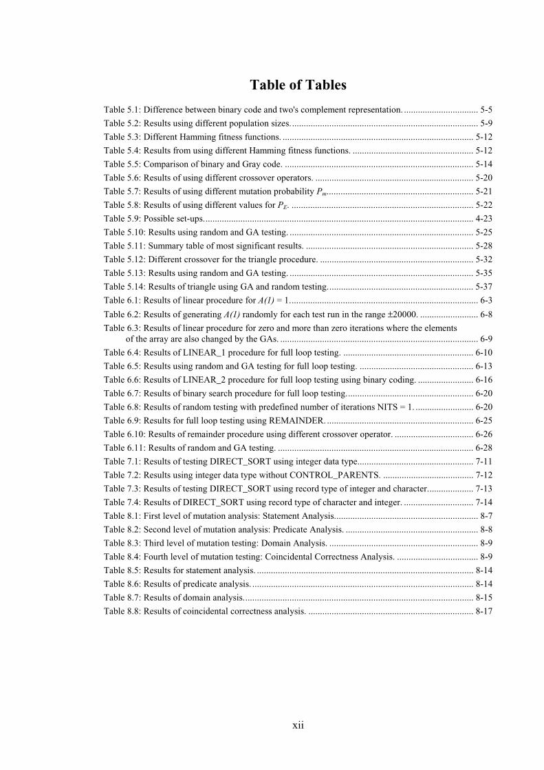
Table of Tables
Table 5.1: Difference between binary code and two's complement representation. ................................ 5-5
Table 5.2: Results using different population sizes................................................................................. 5-9
Table 5.3: Different Hamming fitness functions. .................................................................................. 5-12
Table 5.4: Results from using different Hamming fitness functions. .................................................... 5-12
Table 5.5: Comparison of binary and Gray code. ................................................................................. 5-14
Table 5.6: Results of using different crossover operators. .................................................................... 5-20
Table 5.7: Results of using different mutation probability Pm............................................................... 5-21
Table 5.8: Results of using different values for PE. .............................................................................. 5-22
Table 5.9: Possible set-ups.................................................................................................................... 4-23
Table 5.10: Results using random and GA testing. ............................................................................... 5-25
Table 5.11: Summary table of most significant results. ........................................................................ 5-28
Table 5.12: Different crossover for the triangle procedure. .................................................................. 5-32
Table 5.13: Results using random and GA testing. ............................................................................... 5-35
Table 5.14: Results of triangle using GA and random testing............................................................... 5-37
Table 6.1: Results of linear procedure for A(1) = 1................................................................................. 6-3
Table 6.2: Results of generating A(1) randomly for each test run in the range ±20000. ......................... 6-8Table 6.3: Results of linear procedure for zero and more than zero iterations where the elements
of the array are also changed by the GAs. ..................................................................................... 6-9
Table 6.4: Results of LINEAR_1 procedure for full loop testing. ........................................................ 6-10
Table 6.5: Results using random and GA testing for full loop testing. ................................................. 6-13
Table 6.6: Results of LINEAR_2 procedure for full loop testing using binary coding. ........................ 6-16
Table 6.7: Results of binary search procedure for full loop testing....................................................... 6-20
Table 6.8: Results of random testing with predefined number of iterations NITS = 1. ......................... 6-20
Table 6.9: Results for full loop testing using REMAINDER. ............................................................... 6-25
Table 6.10: Results of remainder procedure using different crossover operator. .................................. 6-26
Table 6.11: Results of random and GA testing. .................................................................................... 6-28
Table 7.1: Results of testing DIRECT_SORT using integer data type.................................................. 7-11
Table 7.2: Results using integer data type without CONTROL_PARENTS. ....................................... 7-12
Table 7.3: Results of testing DIRECT_SORT using record type of integer and character.................... 7-13
Table 7.4: Results of DIRECT_SORT using record type of character and integer. .............................. 7-14
Table 8.1: First level of mutation analysis: Statement Analysis.............................................................. 8-7
Table 8.2: Second level of mutation analysis: Predicate Analysis. ......................................................... 8-8
Table 8.3: Third level of mutation testing: Domain Analysis. ................................................................ 8-9
Table 8.4: Fourth level of mutation testing: Coincidental Correctness Analysis. ................................... 8-9
Table 8.5: Results for statement analysis. ............................................................................................. 8-14
Table 8.6: Results of predicate analysis. ............................................................................................... 8-14
Table 8.7: Results of domain analysis................................................................................................... 8-15
Table 8.8: Results of coincidental correctness analysis. ....................................................................... 8-17

xiii
List of Abbreviations
PC Crossover probability
PS Survive probability
Pm Mutation probability
PSZ Population size
PE Equality probability
Nits Number of iterations
NoRT Number of Random Tests
GA Genetic Algorithm
Pm_w Weighted mutation probability
S Chromosome length
Hx Hamming fitness functionx
C Chromosome
LCSAJ Linear Code Sequence And Jump
CPU Central Processor Unit
MSB Most Significant Bit
LSB Least Significant Bit
F Fitness value
M_G MAX_GENERATION
ES Evolutionstrategie

1-1
CHAPTER 1
Introduction
Between 40% and 50% of the software production development cost is expended in
software testing, Tai [1980], Ince [1987] and Graham [1992]. It consumes resources and
adds nothing to the product in terms of functionality. Therefore, much effort has been
spent in the development of automatic software testing tools in order to significantly
reduce the cost of developing software. A test data generator is a tool which supports
and helps the program tester to produce test data for software.
Ideally, testing software guarantees the absence of errors in the software, but in reality it
only reveals the presence of software errors but never guarantees their absence, Dijkstra
[1972]. Even, systematic testing cannot prove absolutely the absence of errors which are
detected by discovering their effects, Clarke and Richardson [1983]. One objective of
software testing is to find errors and program structure faults. However, a problem might
be to decide when to stop testing the software, e.g. if no errors are found or, how long
does one keep looking, if several errors are found, Morell [1990].
Software testing is one of the main feasible methods to increase the confidence of the
programmers in the correctness and reliability of software, Deason [1991]. Sometimes,
programs which poorly tested, perform correctly for months and even years before some
input sets reveal the presence of serious errors, Miller [1978]. Incorrect software which
is released to market without being fully tested, could result in customer dissatisfaction
and moreover it is vitally important for software in critical applications that it is free of
software faults which might lead to heavy financial loss or even endanger lives, Hamlet
[1987]. In the past decades, systematic approaches to software testing procedures and
tools have been developed to avoid many difficulties which existed in ad hoc
techniques. Nevertheless, software testing is the most usual technique for error detection
in todays software industry. The main goal of software testing is to increase one's
confidence in the correctness of the program being tested.
In order to test software, test data have to be generated and some test data are better at
finding errors than others. Therefore, a systematic testing system has to differentiate

1-2
good (suitable) test data from bad test (unsuitable) data, and so it should be able to
detect good test data if they are generated. Nowadays testing tools can automatically
generate test data which will satisfy certain criteria, such as branch testing, path testing,
etc. However, these tools have problems, when complicated software is tested.
A testing tool should be general, robust and generate the right test data corresponding to
the testing criteria for use in the real world of software testing, Korel [1992]. Therefore,
a search algorithm must decide where the best values (test data) lie and concentrate its
search there. It can be difficult to find correct test data because conditions or predicates
in the software restrict the input domain which is a set of valid data.
Test data which are good for one program are not necessarily appropriate for another
program even if they have the same functionality. Therefore, an adaptive testing tool for
the software under test is necessary. Adaptive means that it monitors the effectiveness of
the test data to the environment in order to produce new solutions with the attempt to
maximise the test effectiveness.
1.1 Objectives and aims of the research project
The overall aim of this research project is to investigate the effectiveness of Genetic
Algorithms (GAs) with regard to random testing and to automatically generate test data
to traverse all branches of software. The objectives of the research activity can be
defined as follows:
• The furtherance of basic knowledge required to develop new techniques for
automatic testing;
• To assess the feasibility of using GAs to automatically generate test data for a variety
of data type variables and complex data structures for software testing;
• To analyse the performance of GAs under various circumstances e.g. large systems.
• Comparison of the effectiveness of GAs with pure random testing for software
developed in ADA;
• The automatic testing of complex software procedures;
• Analysis of the test data adequacy using mutation testing;
The performance of GAs in automatically generating test data for small procedures is
assessed and analysed. A library of GAs is developed and then applied to larger systems.

1-3
The efficiency of GAs in generating test data is compared to random testing with regard
to the number of test data sets generated and the CPU time required.
This research project presents a system for the generation of test data for software
written in ADA83. The problem of test data generation is formed and solved completely
as a numerical optimisation problem using Genetic Algorithms and structural testing
techniques.
Software testing is about searching and generating certain test data in a domain to satisfy
the test criteria. Since GAs are an established search and optimisation process the basic
aim of this project is to generate test sets which will traverse all branches in a given
procedure under test.
1.2 Hypotheses
In order to make my objectives clear several hypotheses are suggested and justified in
the following chapters by evolving experiments which are described in section 4.6.
1. Hypothesis:
Genetic Algorithms are more efficient than random testing in generating test data,
see section 2.2.3. The efficiency will be measured as the number of tests required to
obtain full branch coverage.
2. Hypothesis:
A standard set of parameters for Genetic Algorithms can be established which will
apply to a variety of procedures with different input data types. In particular, the
following will be investigated:
2_1 which of the following bit patterns is most appropriate for representing the
input test-set: twos complement, binary with sign bit or Gray code; see
section 3.7;
2_2 which of the following reproduction strategies is most efficient: selection
at random or according to fitness), see section 3.8.2;
2_3 which crossover strategy is most efficient: single, double or uniform
crossover, see section 3.8.3.1;
2_4 what size of population gives the best result, see section 3.5.1;
2_5 what mutation probability gives the best results, see section 3.5.1.

1-4
These investigations are described in detail in chapter 3. A standard set is
determined in chapter 5 and confirmed in chapters 6 and 7;
3. Hypothesis:
Test cases can be generated for loops with zero, one, two and more than two
iterations, see section 4.7.2. The confirmation is in chapters 6 and 7.
4. Hypothesis:
Genetic Algorithms generate adequate test data in terms of mutation testing and
generating test data for the original (unmutated) software is better. A detailed
description is in section 2.2.1. This is confirmed in chapter 8;
These hypotheses will be under close investigation through out the chapters and will be
discussed in more detail in the chapter 3 and 5 where these different operators and
parameters are introduced.
1.3 Testing criteria
The criterion of testing in this thesis is branch testing, see section 2.1.2. Our aim is to
develop a test system to exercise every branch of the software under test. In order to
generate the required test data for branch testing Genetic Algorithms and random testing
are used. These two testing techniques will be compared by means of the percentage of
coverage which each of them can achieve and by the number of test data which have to
be generated before full branch coverage has been attained.
1.4 Structure of Thesis
Following this introductory chapter, Chapter 2 reviews various testing methods and
applications for software testing. The advantages and disadvantages of these techniques
are examined and explained.
Chapter 3 describes the overall idea of GAs. An introduction to GAs is given and how
and why they work is explained using an example. Various operators and procedures are
explained which are used within a GA. Important and necessary issues of GAs are
described.
Chapter 4 describes the technique which has been applied to test software. A detailed
1-5
description of the application of GAs to software testing is explained and is shown with
brief examples. Instrumentation of the software under test is explained.
The validity of any technique can only be ascertained by means of experimental
verification. A significant part of the work reported in this thesis is the conduct of
experiments which yield results which can be compared to the method of random
testing.
Chapter 5 describes these experiments for a quadratic equation solver procedure and a
triangle classifier procedure using different GAs by means of various settings. These
experiments are conducted in order to investigate the effectiveness of using GA for
software testing. Both procedures under test handle integer variables which are involved
in complex predicates which makes the search for test data difficult. In addition the
triangle procedure comprises various nested procedure declarations.
In Chapter 6, various linear search procedures, a binary search and a remainder
procedure have been tested. Moreover, these procedures have 'loop' conditions as well as
'if' conditions. In contrast to the previous chapter they consist of more complex data
types such as characters, strings and arrays.
Chapter 7 uses a commercially available generic sort procedure, DIRECT_SORT, which
has nested procedure declarations and complex data structures such as records of integer
and character variable arrays where the arrays have to be of variable lenght.
Chapter 8 describes an error - based testing method, also called mutation testing. The
goal is to construct test data that reveal the presence or absence of specific errors and to
measure the adequacy of the test data sets and so of the testing tool.
Chapter 9 gives an overall conclusion of the project. One main conclusion is that the
proposed technique represents a significant improvement over random testing with
regard to the required number of tests. The technique required up to two orders of
magnitude fewer tests and less CPU time.
2-1
CHAPTER 2
Background of various automatic testing methods
Software testing is widely used in many different applications using various testing
strategies. This chapter explains and gives an overview of the fundamental differences
between several approaches to software testing.
2.1 Testing techniques
There are two different testing techniques; black box and white box testing.
2.1.1 Black box testing
In black box testing, the internal structure and behaviour of the program under test is not
considered. The objective is to find out solely when the input-output behaviour of the
program does not agree with its specification. In this approach, test data for software are
constructed from its specification, Beizer [1990], Ince [1987] and Frankl and Weiss
[1993]. The strength of black box testing is that tests can be derived early in the
development cycle. This can detect missing logic faults mentioned by Hamlet [1987].
The software is treated as a black box and its functionality is tested by providing it with
various combinations of input test data. Black box testing is also called functional or
specification based testing. In contrast to this is white box testing.
2.1.2 White box testing
In white box testing, the internal structure and behaviour of the program under test is
considered. The structure of the software is examined by execution of the code. Test
data are derived from the program's logic. This is also called program-based or
structural testing, Roper [1994]. This method gives feedback e.g. on coverage of the
software.
2-2
There are several white box (structural) testing criteria:
• Statement Testing: Every statement in the software under test has to be executed at
least once during testing. A more extensive and stronger strategy is branch testing.
• Branch testing: Branch coverage is a stronger criterion than statement coverage. It
requires every possible outcome of all decisions to be exercised at least once Huang
[1975], i.e. each possible transfer of control in the program be exercised. This means
that all control transfers are executed, Jin [1995]. It includes statement coverage since
every statement is executed if every branch in a program is exercised once. However,
some errors can only be detected if the statements and branches are executed in a
certain order, which leads to path testing.
• Path testing: In path testing every possible path in the software under test is
executed; this increases the probability of error detection and is a stronger method
than both statement and branch testing. A path through software can be described as
the conjunction of predicates in relation to the software's input variables. However,
path testing is generally considered impractical because a program with loop
statements can have an infinite number of paths. A path is said to be 'feasible', when
there exists an input for which the path is traversed during program execution,
otherwise the path is unfeasible.
2.2 Automatic test data generator
Extensive testing can only be carried out by an automation of the test process, claimed
by Staknis [1990]. The benefits are a reduction in time, effort, labour and cost for
software testing. Automated testing tools consist in general of an instrumentator, test
harness and a test data generator.
Static analysing tools analyse the software under test without executing the code, either
manually or automatically. It is a limited analysis technique for programs containing
array references, pointer variables and other dynamic constructs. Experiments have
shown that this kind of evaluation of code inspections (visual inspections) has found
static analysis is very effective in finding 30% to 70% of the logic design and coding
errors in a typical software, DeMillo [1987]. Symbolic execution and evaluation is a
typical static tool for generating test data.
2-3
Many automated test data generators are based on symbolic execution, Howden [1977],
Ramamoorthy [1976]. Symbolic execution provides a functional representation of the
path in a program and assigns symbolic names for the input values and evaluates a path
by interpreting the statements and predicates on the path in terms of these symbolic
names, King [1976]. Symbolic execution requires the systematic derivation of these
expressions which can take much computational effort, Fosdick and Osterweil [1976].
The values of all variables are maintained as algebraic expressions in terms of symbolic
names. The value of each program variable is determined at every node of a flow graph
as a symbolic formula (expression) for which the only unknown is the program input
value. The symbolic expression for a variable carries enough information such that, if
numerical values are assigned to the inputs, a numerical value can be obtained for the
variable, this is called symbolic evaluation. The characteristics of symbolic execution
are:
• Symbolic expressions are generated and show the necessary requirements to execute
a certain path or branch, Clarke [1976]. The result of symbolic execution is a set of
equality and inequality constraints on the input variables; these constraints may be
linear or non-linear and define a subset of the input space that will lead to the
execution of the path chosen;
• If the symbolic expression can be solved the test path is feasible and the solution
corresponds to a set of input data which will execute the test path. If no solution can
be found then the test path is unfeasible;
• Manipulating algebraic expressions is computationally expensive, especially when
performed on a large number of paths;
• Common problems are variable dependent loop conditions, input variable dependent
array (sometimes the value is only known during run time) reference subscripts,
module calls and pointers, Korel [1990];
• These problems slow down the successful application of symbolic execution,
especially if many constraints have to be combined, Coward [1988] and Gallagher
[1993].
Some program errors are easily identified by examining the symbolic output of a
program if the program is supposed to compute a mathematical formula. In this kind of

2-4
event, the output has just to be checked against the formula to see if they match.
In contrast to static analysis, dynamic testing tools involve the execution of the software
under test and rely upon the feedback of the software (achieved by instrumentations) in
order to generate test data. Precautions are taken to ensure that these additional
instructions have no effect whatever upon the logic of the original software. A
representative of this method is described by Gallagher et al. [1993] who used
instrumentation to return information to the test data generation system about the state of
various variables, path predicates and test coverage. A penalty function evaluates by
means of a constraint value of the branch predicate how good the current test data is
with regard to the branch predicate. There are three types of test data generators;
pathwise, data specification and random test data generator.
A test set is run on the software under test, and the output is saved as the actual output of
that test case. The program tester has to examine the output and decides whether it is
correct, by comparing the actual output with the expected-output. If the output is
incorrect, an error has been discovered, the program must be changed and testing must
start again. This leads to regression testing executing all previous test data to verify that
the correction introduced no new errors. BCS SIGIST [1995] defined regression tesing
as:
Retesting of a previously tested program following modification to ensure that faults
have not been introduced or uncovered as a result of the changes made.
To finish testing, the tester will manually examine the output of the test cases to
determine whether they are correct.
Deason [1991] investigated the use of rule-based testing methods using integers and real
variables. His system uses prior tests as input for the generation of additional tests. The
test data generator assigns values directly to input variables in conditions with constants
and then increments and decrements them by small amounts to come closer to the
boundary. The input values are doubled and halved resulting in much faster movements
through the search space. Finally one input variable at a time is set to a random number.
The result of this project is that the rule-based method performed almost always better
than random. Deason called his method multiple-condition boundary coverage where
multiple-condition coverage means that test data exercise all possible combinations of

2-5
condition (true and false) outcomes in every decision. Boundary here means that the test
data has to be as close as possible to switching the conditions from true to false. He
mentioned that it is not possible to generate test data which causes the execution of all
branches in any arbitrary software, i.e. no algorithm exists for solving general non-linear
predicates. In addition, his approach is restricted to numeric types such as integer data
types. A rule based approach has always the drawback that a rule should exist for
unforeseen problems which can be difficult to realise. If such a rule does not exist, the
generation of test data can end in a local optimum solution and not in a global solution
which will traverse a branch.
2.2.1 Pathwise generators
Pathwise test data generators are systems that test software using a testing criterion
which can be path coverage, statement coverage, branch coverage, etc. The system
automatically generates test data to the chosen requirements. A pathwise test generator
consists of a program control flow graph construction, path selection and test data
generation tool.
Deterministic heuristics have been used by Korel [1990, 1992]. He used a dynamic test
data generation approach which is based on a pathwise test data generator to locate
automatically the values of input variables for which a selected path is traversed. His
steps are program control flow graph construction and test data generation. The path
selection stage is not used because if unfeasible paths are selected, the result is a waste
of computational effort examining these paths. Most of these methods use symbolic
evaluation to generate the test data. Korel's method is based on data flow analysis and a
function minimisation approach to generate test data which is based on the execution of
the software under test. Since the software under test is executed, values of array
indexes and pointers are known at each point in the software execution and this
overcomes the problems and limitations of symbolic evaluations.
In Korel's approach a branch function is formed out of the branch predicates where the
control should flow. These functions are dependent on the input variables which can be
difficult to represent algebraically, but the values can be determined by program
execution. The idea is now to minimise these branch functions which have a positive
value when the desired branch is not executed. As soon as the value becomes negative
2-6
the branch will be traversed. The minimisation of the branch function demands that the
path, up to the node where the sibling node should be executed, will be retained for the
next test data.
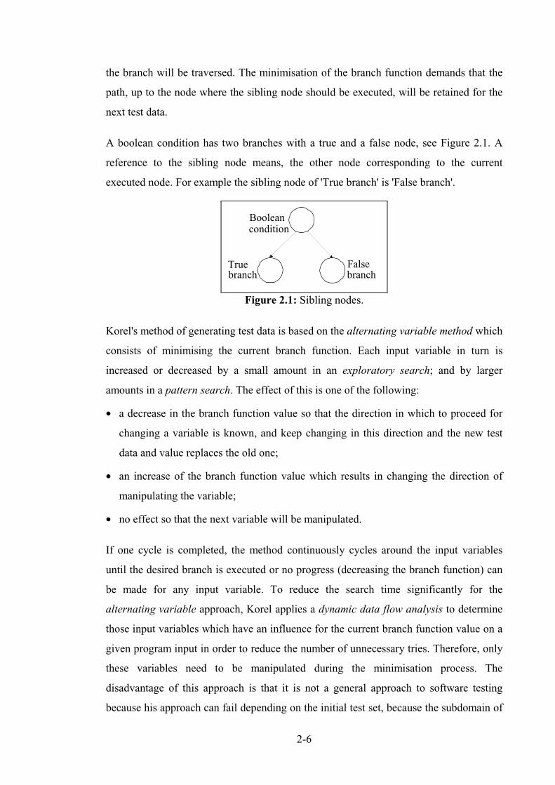
A boolean condition has two branches with a true and a false node, see Figure 2.1. A
reference to the sibling node means, the other node corresponding to the current
executed node. For example the sibling node of 'True branch' is 'False branch'.
Boolean
FalseTrue
condition
branch branch
Figure 2.1: Sibling nodes.
Korel's method of generating test data is based on the alternating variable method which
consists of minimising the current branch function. Each input variable in turn is
increased or decreased by a small amount in an exploratory search; and by larger
amounts in a pattern search. The effect of this is one of the following:
• a decrease in the branch function value so that the direction in which to proceed for
changing a variable is known, and keep changing in this direction and the new test
data and value replaces the old one;
• an increase of the branch function value which results in changing the direction of
manipulating the variable;
• no effect so that the next variable will be manipulated.
If one cycle is completed, the method continuously cycles around the input variables
until the desired branch is executed or no progress (decreasing the branch function) can
be made for any input variable. To reduce the search time significantly for the
alternating variable approach, Korel applies a dynamic data flow analysis to determine
those input variables which have an influence for the current branch function value on a
given program input in order to reduce the number of unnecessary tries. Therefore, only
these variables need to be manipulated during the minimisation process. The
disadvantage of this approach is that it is not a general approach to software testing
because his approach can fail depending on the initial test set, because the subdomain of
2-7
a branch may comprise small and disconnected regions, see e.g. section 5.1 and Figure
5.2. In this case, this local search technique has to be replaced by a global optimisation
technique, otherwise only local minima for the branch function value may be found
which might not be good enough traverse the desired branch. This is where Genetic
Algorithms gain their advantages and strength as a global optimisation process because
they do not depend on a continuous and connected domain.
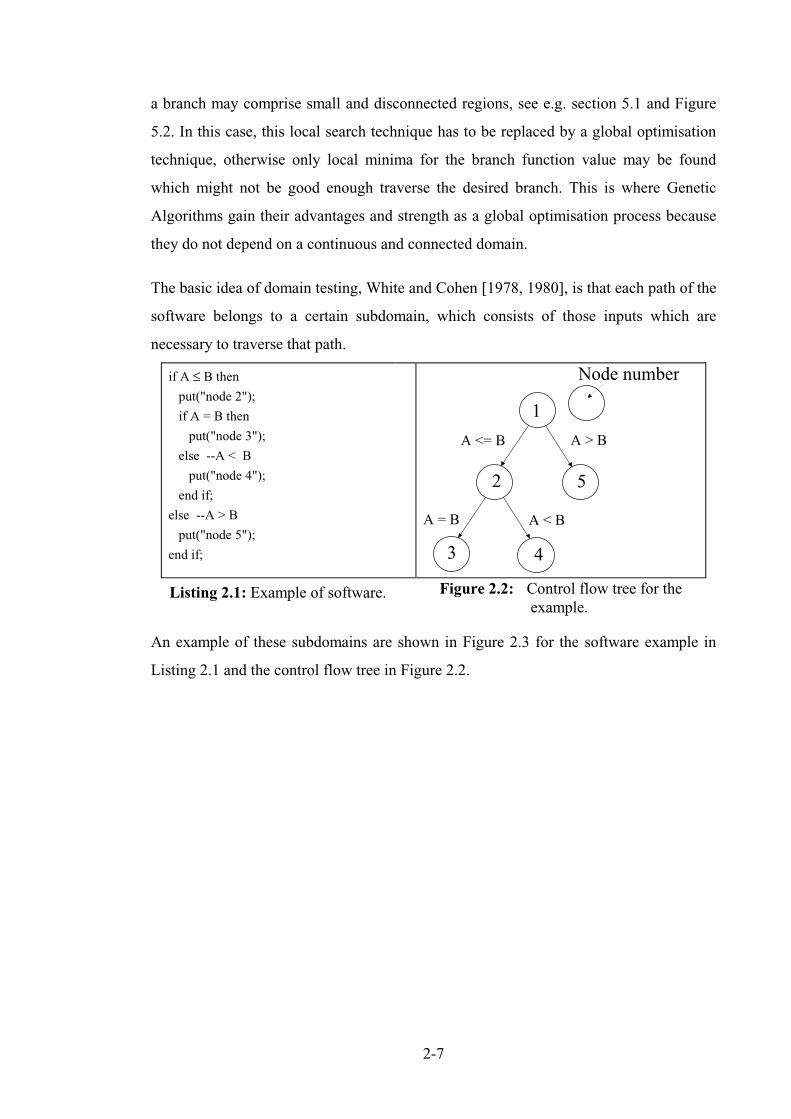
The basic idea of domain testing, White and Cohen [1978, 1980], is that each path of the
software belongs to a certain subdomain, which consists of those inputs which are
necessary to traverse that path.
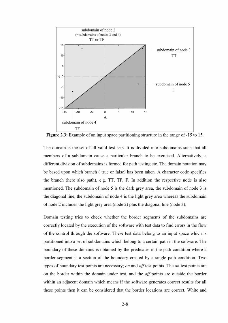
An example of these subdomains are shown in Figure 2.3 for the software example in
Listing 2.1 and the control flow tree in Figure 2.2.
if A ≤ B then
put("node 2");
if A = B then
put("node 3");
else --A < B
put("node 4");
end if;
else --A > B
put("node 5");
end if;
1
2 5
Node number
A = B
A > B
3 4
A < B
A <= B
Listing 2.1: Example of software. Figure 2.2: Control flow tree for theexample.
2-8
-15 -10 -5 0 5 10 15-15
-10
-5
0
5
10
15
A
B
subdomain of node 4
TF
subdomain of node 5
F
subdomain of node 3
TT
subdomain of node 2
TT or TF(= subdomains of nodes 3 and 4)
Figure 2.3: Example of an input space partitioning structure in the range of -15 to 15.
The domain is the set of all valid test sets. It is divided into subdomains such that all
members of a subdomain cause a particular branch to be exercised. Alternatively, a
different division of subdomains is formed for path testing etc. The domain notation may
be based upon which branch ( true or false) has been taken. A character code specifies
the branch (here also path), e.g. TT, TF, F. In addition the respective node is also
mentioned. The subdomain of node 5 is the dark grey area, the subdomain of node 3 is
the diagonal line, the subdomain of node 4 is the light grey area whereas the subdomain
of node 2 includes the light grey area (node 2) plus the diagonal line (node 3).
Domain testing tries to check whether the border segments of the subdomains are
correctly located by the execution of the software with test data to find errors in the flow
of the control through the software. These test data belong to an input space which is
partitioned into a set of subdomains which belong to a certain path in the software. The
boundary of these domains is obtained by the predicates in the path condition where a
border segment is a section of the boundary created by a single path condition. Two
types of boundary test points are necessary; on and off test points. The on test points are
on the border within the domain under test, and the off points are outside the border
within an adjacent domain which means if the software generates correct results for all
these points then it can be considered that the border locations are correct. White and
2-9
Cohen proposed to have two on and one off point where the off point is in between the
two on points. Clarke [1982] extended this technique and suggested having two off
points at the ends of the border under test.
Therefore, domain testing strategies concentrate on domain errors which are based on
the shifting of a border segment by using a wrong relational operator. This means test
data have to be generated for each border segment (predicate) to see whether the
relational operator and the position of the border segment are correct, White and Cohen
[1980] and see chapter 4 for further detail. Hence points close to the border (called
boundary test data) are the most sensitive test data for analysing the path domains and
revealing domain errors, Clarke and Richardson [1983].
Domain testing, therefore, is an example of partition testing. It divides the input space
into equivalent domains and it is assumed that all test data from one domain are
expected to be correct if a selected test data from that domain is shown to be correct.
25% of all errors (bugs) arise out of structural and control flow errors according to
Beizer [1990], pp. 463. Two different types of errors were identified by Howden [1976].
A domain error occurs when a specific input takes the wrong path because of an error in
the control flow of the program which will end in a different subdomain. A
'computational error' is based on an input which follows the correct path, but an error in
some assignment statement causes the wrong output. In complex systems with several
input variables it is usually hard to find data points which belong to a small subdomain
because the subdomain does not have many possible data points. Zeil et al. [1992] and
White and Cohen [1978] used domain testing in their strategies but restrict it to linear
predicates handling floating point variables. They use a symbolic analysis for the paths
and a geometrical approach for test data generation. An example is in chapter 4 of
generating test data using Genetic Algorithms to check these subdomains and
boundaries of a small program.
Mutation testing is an implementation of an error-based testing method, DeMillo [1978].
It is based on the introduction of a single syntactically-correct fault e.g. by manipulation
of conditions and statements. This new program is called mutant. Mutation testing is
used to show the absence of prespecified faults, Morell [1990]. After checking the
output of the original program to be correct (by some oracle), the same test data is input
2-10
to the mutant and if the output of the mutant differs from the expected output the mutant
is killed by the test data because the error is detected. If the mutant has not been killed
and it is said to be still alive and more test data have to be generated to kill it. If a mutant
cannot be killed then either it is an equivalent mutant (no functional change) or the test
data sets are not of sufficient quality. This revealed a weakness in the test data (low
quality test data). By using test data which do not kill the mutants, it can be said that
either the generating tool for test data is not good enough and the original program has
to be re-examined or additional test data have to be produced until some threshold is met
where it appears that it is impossible to reveal a difference. The checking of the
correctness is a major factor in the high cost of software development. Checking
correctness of test data can be automated by using an oracle or post conditions, Holmes
[1993] or from input - output specification. The main task is to generate test data that
reveals a difference in the mutant's behaviour corresponding to the original software. A
detailed description and application is given in chapter 8. Mutation testing shows only
the absence of certain faults. However, it is very time consuming to generate and test a
large number of mutant programs. Hypothesis 4 is formulated which states that GAs are
robust to generate test data and that it is better to generate test data for the original or the
mutant program.
2.2.2 Data specification generators
Deriving test data from specification belongs to the 'black-box' testing method. Such a
strategy generate test cases and test data e.g. from formal Z specification, Yang [1995].
The test data can then be applied to software and the effectiveness can be measured, e.g.
using ADATEST (ADATEST is an automatic testing system for Ada software which
measures for example the percentage of statements executed or branches covered).
A disadvantage is the need for a formal specification for the software which does not
often exist, Gutjahr [1993].
2.2.3 Random testing
Random testing selects arbitrarily test data from the input domain and then these test
data are applied to the program under test. The automatic production of random test
data, drawn from an uniform distribution, should be the default method by which other
2-11
systems should be judged, Ince [1987]. Statistical testing is a test case design technique
in which the tests are derived according to the expected usage distribution profile.
Taylor [1989], Ould [1991] and Duran [1981] suggested that the distribution of selected
input data should have the same probability distribution of inputs which will occur in
actual use (operational profile or distribution which occurs during the real use of the
software) in order to estimate the operational reliability.
Hamlet [1987] mentioned that the operational distribution for a problem may not be
known and a uniform distribution may choose points from an unlikely part of the
domain which can lead to inaccurate predictions, however, he still favours this
technique. Duran [1981] had the opinion that an operational profile is not as effective
for error detection as a uniform distribution. Taylor [1989] mentioned that concentrating
on a certain feature using partition testing tended to be easier and simpler to generate
test data than actual user inputs (operational profile) because they are focused on a
particular feature. Partitioning testing is less effective than random testing in detecting
faults which cause a printer controller to crash, Taylor [1989]. Random testing is the
only standard in reliability estimation, Hamlet and Taylor [1990], in the user application
because it can use data which resemble the user's operational profile. Partition testing in
general can not supply this information because it focuses on test data in partitions that
are more likely to fail, so that the failure rate for partition testing would be higher than
that in expected actual use. If it is not known where the faults are likely to be, partition
testing is not significantly better than random testing.
Hamlet and Taylor [1990] mentioned that there is not much difference between partition
and random testing in terms of finding faults. Hamlet showed that random testing is
superior to partition testing with regard to human effort especially with more partitions
and if confidence is required. For a small number of sub-domains partition testing will
perform better than random testing.
On the contrary Deason [1991] commented that random number generators are
ineffective in that they rarely provide the necessary coverage of the program. Myers
[1979] strengthened this comment and is of the opinion that random testing is probably
the poorest methodology in testing. However, Duran and Ntafos [1984] and Duran
[1981] stated that many errors are easy to find, but the problem is to determine whether a
2-12
test run failed. Therefore, automatic output checking is essential if large numbers of tests
are to be performed. They also said that partition testing is more expensive than
performing an equivalent number of random tests which is more cost effective because it
only requires a random number generator and a small amount of software support.
DeMillo [1978] proved that the adequacy of random data is very dependent on the
interval (range) from which the data is generated. Data from poorly chosen intervals are
much worse than those from well chosen intervals. Duran and Ntafos [1984] agreed that
the change of range for random testing has a great effect. Further they mentioned a
disadvantage of random testing which is to satisfy equality values which are difficult to
generate randomly.
Moranda [1978], Bertolino [1991] commented, the advantage of random testing is
normally that it is more stressing to the program under test than hand selected test data,
but on the other hand random inputs may never exercise both branches of a predicate
which tests for equality. Even in the case that random testing is cheaper than partition
testing, the slight advantage of random testing could be compensated for by using more
random tests and there is no assurance that full coverage can be obtained, e.g. if equality
between variables are required. And secondly it may mean examining the output from
thousands of tests.
Random testing was especially recommended for the final testing stage of software by
Tsoukalas [1993] and Girard and Rault [1973]. Duran and Ntafos [1984] recommended
a mixed final testing, starting with random testing, followed by a special value testing
method (to handle exceptional cases). Ince [1986] reported that random testing is a
relatively cheap method of generating initial test data.
It is decided to use random testing as a benchmark for our Genetic Algorithm testing
system as suggested by Ince [1987]. It offers a good comparison between the systems so
that also other testing tool system can be easily compared indirectly to our system.
Whether the comparism of GA's with random testing is appropriate, especially when
generating test data for disconnected subdomains, will be examined and discussed in
chapters 5, 6, 7 and 8. Therefore, the hypothesis 1 is formulated, see section 1.2. Are
using GAs in order to generate test data more effective than using random testing?

2-13
The next chapter explains the method of Genetic Algorithms and their features and
characteristics. An example shows the method of working of the GAs.
3-1
CHAPTER 3
Genetic Algorithm
Optimisation problems arise in almost every field, especially in the engineering world.
As a consequence many different optimisation techniques have been developed.
However, these techniques quite often have problems with functions which are not
continuous or differentiable everywhere, multi-modal (multiple peaks) and noisy.
Therefore, more robust optimisation techniques are under development which may be
capable of handling such problems. In the past biological and physical approaches have
become of increasing interest to solve optimisation problems, including for the former
neural networks, genetic algorithms and evolution strategies (ESs) and for the second
simulated annealing, Hills and Barlow [1994], Rayward-Smith and Debuse [1994],
Bayliss [1994], Golden and Skiscim [1986], Hoffmann et al. [1991], Osborne and Gillett
[1991].
Other optimisation techniques are:
• Tabu search, Glover [1989], Reeves et al. [1994], Rayward-Smith and Debuse
[1994];
• Simplex method, Box [1965];
• Hooke Jeeves, Hooke and Jeeves [1961];
• Gradient method, Donne et al. [1994].
This chapter explains the features and methods of Genetic Algorithms. An introduction
to genetic algorithms is followed by an optimisation example using genetic algorithms.
3.1 Introduction to Genetic Algorithms
Genetic algorithms (GAs) represent a class of adaptive search techniques and procedures
based on the processes of natural genetics and Darwin's principal of the survival of the
fittest. There is a randomised exchange of structured information among a population of
artificial chromosomes. GAs are a computer model of biological evolution. When GAs
are used to solve optimisation problems, good results are obtained surprisingly quickly.
In the context of software testing, the basic idea is to search the domain for input

3-2
variables which satisfy the goal of testing.
3.2 Application of Genetic Algorithms
Creatures are the perfect problem solver. In the amount of tasks which they have to cope
with (e.g. adaptation, changing environment), they do better by far than the best
computer programs to the frustration of programmers because these organisms acquire
their ability by the apparently aimless mechanism of evolution.
GAs have been used in many different applications as an adaptive search method, e.g. by
Grefenstette et al. [1985 a], Allen and Lesser [1989], and Jog et al. [1989].
The fundamental concept of GAs is to evolve successive generations of increasingly
better combinations of those parameters which significantly effect the overall
performance of a design. The GAs come from the evolution strategy. Perhaps the
slowness of biological evolution has lead to the fallacy that evolution strategies are in
principle time consuming and less efficient.
However, the Berlin Professor for the science of engineering, Rechenberg, successfully
developed independently and applied a selection - mutation - strategy, with the name
Evolutionstrategie (ES), on the basis of trial and error principle in the early 1960s.
Rechenberg [1965] and Schwefel [1989] developed an optimal solid shape for the flow
technique and achieved astonishing shapes for a nozzle which are distinguished by their
high efficiency. Mutation was the key operator in his investigation. He also applied ES
to determine the optimum configuration of five plates of steel in which each of them
could have fifty one different positions corresponding to a search space consisting of
some 3.45x10⁸ plate configurations. An optimal solution was achieved by using the ES.
By selecting an experiment with a known optimal solution Rechenberg successfully
demonstrated the capabilities of an evolutionary algorithm.
This result is very impressive because the experimental method was quite simple and the
mathematical approach failed due to the complexity. The disadvantage of a random
method which is that no step builds upon another is avoided by using these evolution
strategies. Its steps are based on the experience which has been gained from previous
trials, Abblay [1987]. Many other projects have used evolutionary strategies, among
them are the development of a right-angled pipe with minimum flow resistance and

3-3
other structural elements Parmee [1992].
A parallel development of evolutionary algorithms has also taken place in the USA.
Seminal work concerning the formulation and behaviour of GAs was pioneered by
Holland [1975] in his research on adaptation in natural and artificial systems at the
University of Michigan (USA). Three basic operators are responsible for GAs: selection,
crossover and mutation. The main genetic operator is crossover which performs
recombination (mixing) of different solutions to ensure that the genetic information of a
child life form is made up of the elements (genes) from each parent. He simulated the
methods used when biological systems adapt to their environment in computer software
models to solve optimisation problems. Also in the former USSR the method of
evolution has been an accepted technique for many years, Zhigljavsky [1991].
Evolution avoids one of the most difficult obstacles which the software designer is
confronted: the need to know in advance what to do for every situation which may
confront a program. The advantage of GAs is the fact that they are adaptive. These GAs
have already achieved epoch-making solutions for complex tasks like the construction of
an aeroplane turbine. Evolution is under the influence of two fundamental processes;
natural selection and recombination. The former determines which individual member of
a population is selected, survives and reproduces, the latter ensures that the genes (or
entire chromosome) will be mixed to form a new one. Human beings have used a
combination of crossbreeding and selection, to breed more productive corn, faster
racehorses or more beautiful roses for thousands of years, Holland [1992].
Goldberg [1989] mentioned that various engineering projects had applied GAs to solve
problems, e.g. to optimise a gas pipeline control. This problem was controlled by non-
linear state transition equations that impose the pressure drop through the pipelines and
pressure rise across compressors.
Other applications describe the use of GAs to the optimisation of a ten member plane
truss, Goldberg and Samtani [1986]. The objective of this problem is to minimise the
weight of the structure under the condition of maximum and minimum stress constraints
on each member. As reported the GA always showed optimal solutions.
Grefenstette and Fitzpatrick [1985 b] considered a medical imaging system problem
3-4
where the problem lies in the registration of digital images. The functions which are to
be optimised in image registration are the measures of the difference between (in this
case) two x-ray images, one taken prior to the injection of dye into the artery and one
taken following the injection. The images differ because of motion which has taken
place between the two acquisition times. The two images are digitised and subtracted
pixel by pixel with the desired end result being a difference image that clearly outlines
the interior of the subject artery. By performing a geometrical transformation which
warps one image relative to the other it is possible to improve the registration of the
images so that the difference which is due to the motion is reduced.
GAs are also applied to the classical problem of the Prisoner's Dilemma problem,
studied by Mühlenbein [1991 a], Fujiki and Dickinson [1987] and Wilson [1987]. In its
simplest form, each of the two players have a choice of co-operating with the other or
defecting. Grefenstette et al. [1985 b] and Oliver et al. [1987] applied GAs to the well
known combinatorial optimisation Travelling Salesman Problem (TSP). The
optimisation problem consists in finding the shortest distance (normally Euclidean
distance) between n cities. Shultz et al. [1992, 1993] used GA in order to test
autonomous vehicle software controllers. The task for this application is to search for
combinations of faults that produce abnormal vehicle controller performance by
comparing a controller to a chosen set of fault scenarios within a vehicle simulator. They
concluded that this approach using GA is an effective method compared to manual
testing of sophisticated software controllers.
In addition, GAs have been applied to the optimisation for example of the design of a
concrete shell of an arch dam (large scale hydropower scheme) Parmee [1994]; the
design of digital filters, Suckley [1991], Roberts and Wade [1994]; the design of cooling
hole geometry of gas turbine blades, Parmee et al. [1993], Parmee and Purchase [1991];
design of microwave absorbers (low-profile radar absorbing materials) which results in a
reduction of the radar signature of military hardware, Tennant and Chambers [1994] and
the generation of test patterns for VLSI circuits, O'Dare et al. [1994].
3.3 Overview and basics of Genetic Algorithms
GAs offer a robust non-linear search technique that is particularly suited to problems
involving large numbers of variables. The GA achieves the optimum solution by the
3-5
random exchange of information between increasingly fit samples and the introduction
of a probability of independent random change. Compared to other search methods,
there is a need for a strategy which is global, efficient and robust over a broad spectrum
of problems. The strength of GAs is derived from their ability to exploit in a highly
efficient manner, information about a large number of individuals. This search method is
modelled on natural selection by Holland [1992] whose motivation was to design and
implement a robust adaptive system. GAs are being used to solve a variety of problems
and are becoming an important tool in machine learning and function optimisation,
Goldberg [1989]. Natural selection is used to produce adaptation.
GAs derive their name from the fact that they are loosely based on models of genetic
change in a population of individuals, in order to effect a search mechanism with
surprising power and speed. These algorithms apply genetically inspired operators to
populations of potential solutions in an iterative fashion, creating new populations while
searching for an optimum solution. The key word here is population. The fact that many
points in the space are sampled in parallel shows that genetic algorithms are a global
optimisation technique. GAs do not make incremental changes to a single structure, but
maintain a population of structures from which new structures are created using genetic
operators. The evolution is based on two primary operators: mutation and crossover.
The power of genetic algorithms is the technique of applying a recombination operator
(crossover and mutation) to a population of individuals. Despite their randomised nature,
GAs are not a simple random search. GAs take advantage of the old knowledge held in a
parent population to generate new solutions with improved performance. Thereby, the
population undergoes simulated evolution at each generation. Relatively good solutions
reproduce; relatively bad ones die out and are replaced by fitter offspring.
An important characteristic of genetic algorithms is the fact that they are very effective
when searching or optimising spaces that are not smooth or continuous. These are very
difficult or impossible to search using calculus based methods, e.g. hill climbing.
Genetic algorithms may be differentiated from more conventional techniques by the
following characteristics:
1. A representation for the sample population must be derived;
2. GAs manipulate directly the encoded representation of variables, rather than
3-6
manipulation of the variables themselves;
3. GAs use stochastic rather then deterministic operators;
4. GAs search blindly by sampling and ignoring all information except the outcome of
the sample;
5. GAs search from a population of points rather than from a single point, thus
reducing the probability of being stuck at a local optimum which make them suitable
for parallel processing, see section 3.5;
GAs are iterative procedures that produce new populations at each step. A new
population is created from an existing population by means of performance evaluation,
selection procedures, recombination and survival. These processes repeat themselves
until the population locates an optimum solution or some other stopping condition is
reached, e.g. number of generation or time.
The initial population comprises a set of individuals generated randomly or heuristically.
The selection of the starting generation has a significant effect on the performance of the
next generation. In most GAs, individuals are represented by a fixed-length string over a
finite alphabet. The binary alphabet is one of many possible ways of representing the
individuals. GAs work directly with this representation and they are difficult to fool
because they are not dependent upon continuity of the parameter space and existence of
a derivative.
The process is similar to a natural population of biological creatures where successive
generations are conceived, born and raised until they themselves are ready to reproduce.
This population-by-population approach is very different from the more typical search
methods of engineering optimisation. In many search methods, we move gingerly from a
single point in the decision space to the next, using some decision rule to tell us how to
get to the next point (hill climbing). This point-by-point method is dangerous because it
often locates local peaks in the search space. GAs work from a population of points
(individuals) simultaneously climbing many peaks in one generation (parallel), thus
reducing the probability of finding a local optimum. To get a starting population, we can
generate a number of strings at random, or if we have some special prior knowledge of
good regions of the decision space, we may plant seeds within the population to help
things along. Regardless of the starting population, the operators of genetic algorithm
3-7
have found members of high fitness quickly in many applications studied to date.
A string of a population can be considered as concatenated sub-strings (input variables)
to represent a chromosome. The individual bits of the string represent genes. The length
of a string is S and a population of strings contains a total of PSZ strings.
Once the initial population has been created the evaluation phase begins. The GAs
require that members of the population can be differentiated according to the string's
fitness. The parameter combinations are then processed by a model of the system under
test. The relative fitness of each combination is determined from the model's output.
Fitness is defined as a non negative function which is to be maximised. An increase in
the population average fitness is the overall effect of genetic algorithms.
The members that are fitter are given a higher probability of participating during the
selection and reproduction phases and the others are more likely to be discarded. Fitness
is measured by decoding a chromosome in the corresponding variables to an objective
function (which is specific to the problem being solved). The value returned by the
objective function is used to calculate a fitness value. The fitness is the only feedback
facility which maintains sufficient selective differences between competing individuals
in a population stated by DeJong [1993]. The genetic algorithms are blind; they know
nothing of the problem except the fitness information.
In the selection phase, chromosomes of the population may be chosen for the
reproduction phase in several ways: for example, they may be chosen at random, or
preference may be given to the fitter members.
During the reproduction phase, two members are chosen from the generation. The
evolutionary process is then based on the genetic or recombination operators, crossover
and mutation, which are applied to them to produce two new members (offspring) for
the next generation.
The crossover operator couples the items of two parents (chromosomes) to generate two
similar offspring, which are created by swapping corresponding substrings of its parents.
The idea of crossover is to create better individuals by combining genetic material
(genes) of fitter parents. The mutation operator alters one or more genetic cells (genes)
of a selected structure with a low probability. This ensures a certain diversity in the
3-8
genetic chromosomes over long periods of time and prevents stagnation near a local
optimum. This means a complete new population of offspring is formed. A predefined
survival strategy determines which of the parent and offspring survive.
The whole process is repeated generation by generation until a global optimum is found
or some other stopping condition is reached. One of the disadvantages can be the
excessive number of iterations required and therefore the amount of computational time.
3.4 Features of GAs
GAs are quite successful in solving problems of the type that are too constrained for
more conventional strategies like hill climbing and derivative based techniques. A
problem is to maximise a function of the kind f(x1, x2, ..., xm) where (x1, x2, ..., xm) are
variables which have to be adjusted towards a global optimum. The bit strings of the
variables are then concatenated together to produce a single bit string (chromosome)
which represents the whole vector of the variables of the problem. In biological
terminology, each bit position represents a gene of the chromosome, and each gene may
take on some number of values called alleles.
In the following sections the method of GAs is explained and how and why they work.
The basic structure, a variety of operators and control parameters are explained. An
example will be taken of a function which is to be optimised. An explanation regarding
the population and chromosome, fitness, selection, crossover, mutation and survival
procedure will be given.
3.5 Population and generation
A population is like a list of several guesses (database). It consists of information about
the individuals. As in nature, a population in GAs has several members in order to be a
healthy population. If the population is too small inbreeding could produce unhealthy
members. DeJong [1988] mentioned that the population size should be generally in the
range of 50 - 100 members, although we find out that a different size can be beneficial,
see section 6.1.1.2. The population changes from one generation to next. The individuals
in a population represent solutions. The advantage of using a population with many
members is that many points in a space are searched in one generation. GAs are
3-9
therefore highly suited for parallel processing, Robertson [1987], Mühlenbein [1989],
Georges-Schleuter [989] and Goldberg [1989]. This sets the GAs apart from other
search methods.
3.5.1 Convergence and sub optima solutions
A generation is said to have premature by converged when the population of a
generation has a uniform structure at all positions of the genes without reaching an
optimal structure, Baker [1985]. This means that the GA or the generation has lost the
power of searching and generating more better solutions.
As we shall see later in 5.1.4, generally small populations can quickly find good
solutions because they require less computational effort (fewer evaluations per
generation). However, premature convergence is generally obtained in a small
population and the effect is that the population is often stuck on a local optimum. This
can be compensated by an increased mutation probability, see section 5.18, which would
be similar to a random testing method. Larger populations are less likely to be caught by
local optima, but generally take longer to find good solutions and an excessive amount
of function evaluation per generation is required. A larger population allows the space to
be sampled more thoroughly, resulting in more accurate statistics. Samples of small
populations are not as thorough and produce results with a higher variance. Therefore, a
method must be set up in order to find a strategy which will avoid converging towards a
non optimum solution. Hypothesis 2_4 (see section 1.2), therefore, investigates the size
of a population. Hypothesis 2_5 studies the percentage of probability of mutation on
average per chromosome.
3.6 Seeding
In order to start the optimisation method, the first population has to be generated. It can
be seeded with a set of parameter values which can influence the search through the
space. It can help to speed up the location of an optimum. Some systems have used
parameter values from the previous experiments to provide a portion of the initial
population, Powell [1989]. Alternatively values can be used which the user believes are
in the right area of the search space to find an optimum faster. Normally the seeding is
performed by random selection which means that random data are generated.
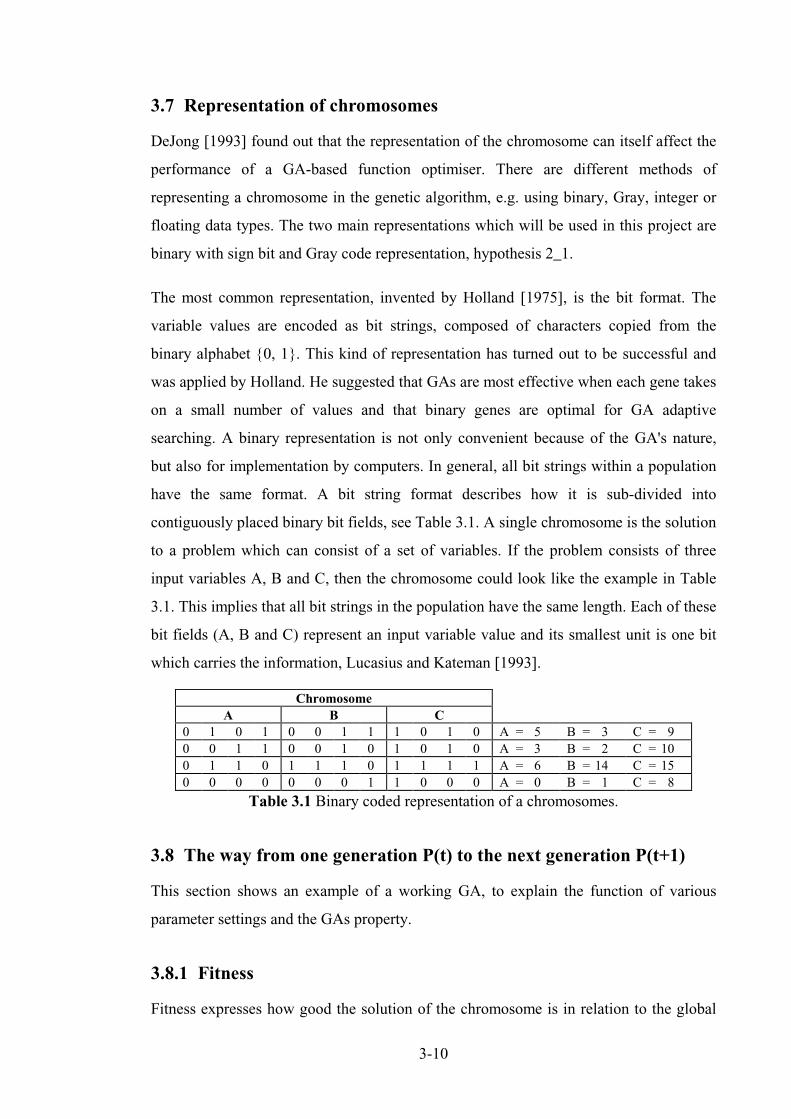
3-10
3.7 Representation of chromosomes
DeJong [1993] found out that the representation of the chromosome can itself affect the
performance of a GA-based function optimiser. There are different methods of
representing a chromosome in the genetic algorithm, e.g. using binary, Gray, integer or
floating data types. The two main representations which will be used in this project are
binary with sign bit and Gray code representation, hypothesis 2_1.
The most common representation, invented by Holland [1975], is the bit format. The
variable values are encoded as bit strings, composed of characters copied from the
binary alphabet {0, 1}. This kind of representation has turned out to be successful and
was applied by Holland. He suggested that GAs are most effective when each gene takes
on a small number of values and that binary genes are optimal for GA adaptive
searching. A binary representation is not only convenient because of the GA's nature,
but also for implementation by computers. In general, all bit strings within a population
have the same format. A bit string format describes how it is sub-divided into
contiguously placed binary bit fields, see Table 3.1. A single chromosome is the solution
to a problem which can consist of a set of variables. If the problem consists of three
input variables A, B and C, then the chromosome could look like the example in Table
3.1. This implies that all bit strings in the population have the same length. Each of these
bit fields (A, B and C) represent an input variable value and its smallest unit is one bit
which carries the information, Lucasius and Kateman [1993].
Table 3.1 Binary coded representation of a chromosomes.
3.8 The way from one generation P(t) to the next generation P(t+1)
This section shows an example of a working GA, to explain the function of various
parameter settings and the GAs property.
3.8.1 Fitness
Fitness expresses how good the solution of the chromosome is in relation to the global
ChromosomeA B C
0 1 0 1 0 0 1 1 1 0 1 0 A = 5 B = 3 C = 90 0 1 1 0 0 1 0 1 0 1 0 A = 3 B = 2 C = 100 1 1 0 1 1 1 0 1 1 1 1 A = 6 B = 14 C = 150 0 0 0 0 0 0 1 1 0 0 0 A = 0 B = 1 C = 8

3-11
optimum. This kind of value will be calculated for each chromosome in each population
by a fitness function. The fitness value is used to compare the individuals and to
differentiate their performance. An individual which is near an optimum solution gets a
higher fitness value than an individual which is far away. The fitness value is the only
feedback from the problem for the GA. The GA does not need any knowledge about the
problem and it is blind in all other respects. A difficult issue in using GA is often the
attempt to find a suitable fitness function which calculates the fitness value, and
expresses the problem as well as possible. Every point in the search space must be
represented by a valid fitness value.
For example , suppose that the function to optimise is f A A( ) = 2 with ( [ , ])A ∈ 0 15 and
the fitness function has in this case the same form:
fitness Ai = 2 (4.1.)
The initial population is generated randomly. The population will only consist of one
input variable per chromosome and four individuals per generation.
Table 3.2: Chromosomes with fitness values for the initial population.
Table 3.2 shows the chromosomes with their fitness values calculated by the fitness
function (4.1). The total fitness of the population is calculated in equation (4.2):
fitness ftotal ii
= ==� 71
1
4
(4.2)
The higher the fitness value, the better and closer the individual is towards the global
optimum, which is in this case a value of A = 15 .
3.8.2 Selection
The selection operator chooses two individuals from a generation to become parents for
the recombination process (crossover and mutation). There are different methods of
selecting individuals, e.g. randomly or with regard to their fitness value. This issue is
Chromosome Ai Fitness (fi)
C1 5 25C2 3 9C3 6 36C4 1 1
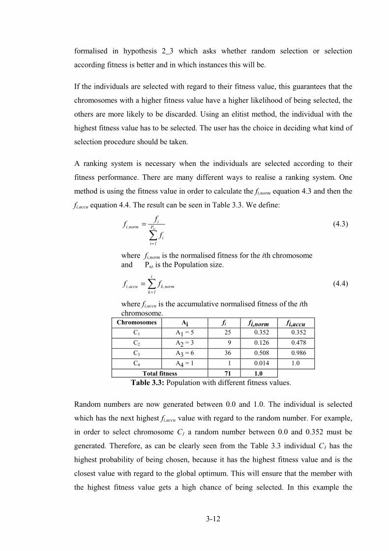
3-12
formalised in hypothesis 2_3 which asks whether random selection or selection
according fitness is better and in which instances this will be.
If the individuals are selected with regard to their fitness value, this guarantees that the
chromosomes with a higher fitness value have a higher likelihood of being selected, the
others are more likely to be discarded. Using an elitist method, the individual with the
highest fitness value has to be selected. The user has the choice in deciding what kind of
selection procedure should be taken.
A ranking system is necessary when the individuals are selected according to their
fitness performance. There are many different ways to realise a ranking system. One
method is using the fitness value in order to calculate the fi,norm equation 4.3 and then the
fi,accu equation 4.4. The result can be seen in Table 3.3. We define:
ff
fi norm
i
ii
Psz, =
=�
1
(4.3)
where fi,norm is the normalised fitness for the ith chromosomeand Psz is the Population size.
f fi accu k normk
i
, ,==�
1
(4.4)
where fi,accu is the accumulative normalised fitness of the ithchromosome.
Table 3.3: Population with different fitness values.
Random numbers are now generated between 0.0 and 1.0. The individual is selected
which has the next highest fi,accu value with regard to the random number. For example,
in order to select chromosome C1 a random number between 0.0 and 0.352 must be
generated. Therefore, as can be clearly seen from the Table 3.3 individual C3 has the
highest probability of being chosen, because it has the highest fitness value and is the
closest value with regard to the global optimum. This will ensure that the member with
the highest fitness value gets a high chance of being selected. In this example the
Chromosomes Ai fi fi,norm fi,accuC1 A1 = 5 25 0.352 0.352
C2 A2 = 3 9 0.126 0.478
C3 A3 = 6 36 0.508 0.986
C4 A4 = 1 1 0.014 1.0
Total fitness 71 1.0

3-13
individual with the index number C3, C1, C2 and C3 are selected, as shown in Table 3.4.
Individual C3 has been selected twice. This is justified by its high fitness value f3, which
also has the biggest range of the normalised accumulated fitness value (f3,accu
- f2,accu).
Individual C4 which has the smallest fitness value and, therefore, the smallest range of
the normalised accumulated value has not been selected.
Table 3.4: Selected chromosomes after selection procedure.
Selection procedures which will be investigated in further experiments are described in
the following sections.
3.8.2.1 Selection according to fitness
This select procedure SELECT_F (uppercase names are names of procedures) will select
the parents according to their fitness value, see Table 3.5. The advantage of this method
is to prefer the fitter members of the population in order to guarantee that the best
members are chosen with regard to fitness. The offspring should have increased fitness
which means that they are closer to the global optimum.
Table 3.5: Pseudo code of procedure SELECT_F.
3.8.2.2 Random selection
The selection of the parents could be made randomly using SELECT_R, so that every
member of the population has an equal chance of being selected for recombination, see
Table 3.6.
Table 3.6: Pseudo code of procedure SELECT_R.
This method would guarantee diversity and healthy mating. Selecting only members
Random numbers 0.8547 0.1258 0.4317 0.9416Chromosomes C3 C1 C2 C3
Provide the normalised accumulated fitness for offspring population;for population size loop;
rand = random number;loop
if rand ≤ Foffspring, i, accu thenselect this offspring individual;exit loop;
end if;end loop;
rand = random number;select this offspring individual;

3-14
with a high fitness (SELECT_F) can lead to inbreeding which can cause strong
convergence towards a local optimum and a loss on diversity. It can be difficult to leave
that local optimum in order to find the global optimum. A pseudo random number
generator is used with uniform distribution to select the members of a generation to
become parents for the mating process.
3.8.3 Recombination operators
These operators, crossover and mutation, are the key to the power of GAs. They are the
operators which create new individuals with the idea that the new individuals will be
closer to a global optimum.
3.8.3.1 Crossover operator
Crossover operates at the individual level. Before the crossover operator may be applied,
the individual can be converted into a binary representation. During crossover, the two
parents (chromosomes) exchange sub string information (genetic material) at a random
position in the chromosome to produce two new strings (offspring). The crossover
operators search for better genes (building blocks) within the genetic material. The
objective here is to create better individuals and a better population over time by
combining material from pairs of (fitter) members from the parent population. Crossover
occurs according to a crossover probability PC. The easiest form of crossover is the
single crossover operator. This matter will be investigated in Hypothesis 2_3 to find the
optimum crossover operator.
3.8.3.1.1 Single crossover
A crossover point is randomly chosen for two chromosomes (parents). This point occurs
between two bits and divides each individual into left and right sections. Crossover then
swaps the left (or right) section of two individuals which can be seen in Figure 3.1. For
example, if the two parents are [v1,...,vm] and [w1,...,wm], then crossing the chromosomes
after the kth gene (1 ≤ ≤k m ) would produce the offspring: [v1,...,vk,wk+1,...,wm] and
[w1,...,wk,vk+1,...,vm].
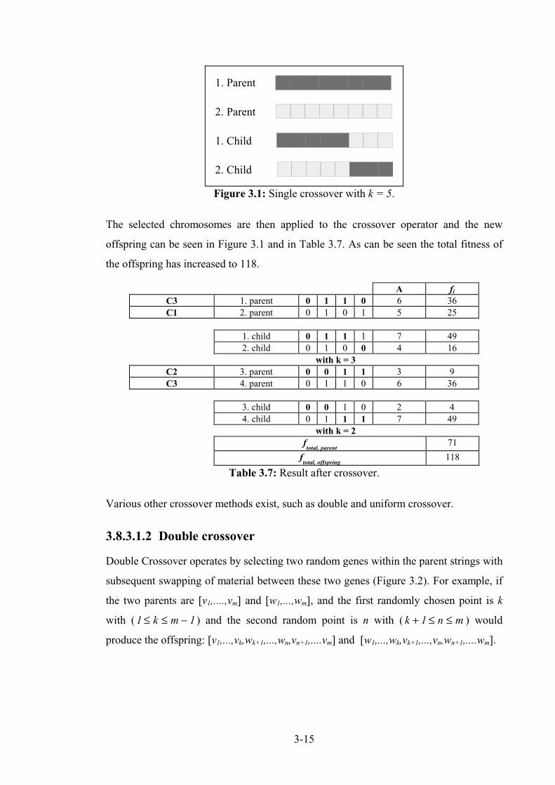
3-15
1. Parent
2. Parent
1. Child
2. Child
Figure 3.1: Single crossover with k = 5.
The selected chromosomes are then applied to the crossover operator and the new
offspring can be seen in Figure 3.1 and in Table 3.7. As can be seen the total fitness of
the offspring has increased to 118.
Table 3.7: Result after crossover.
Various other crossover methods exist, such as double and uniform crossover.
3.8.3.1.2 Double crossover
Double Crossover operates by selecting two random genes within the parent strings with
subsequent swapping of material between these two genes (Figure 3.2). For example, if
the two parents are [v1,....,vm] and [w1,...,wm], and the first randomly chosen point is k
with (1 1≤ ≤ −k m ) and the second random point is n with ( k n m+ ≤ ≤1 ) would
produce the offspring: [v1,...,vk,wk+1,...,wn,vn+1,....vm] and [w1,...,wk,vk+1,...,vn,wn+1,....wm].
A fiC3 1. parent 0 1 1 0 6 36C1 2. parent 0 1 0 1 5 25
1. child 0 1 1 1 7 492. child 0 1 0 0 4 16
with k = 3C2 3. parent 0 0 1 1 3 9C3 4. parent 0 1 1 0 6 36
3. child 0 0 1 0 2 44. child 0 1 1 1 7 49
with k = 2ftotal, parent
71
ftotal, offspring
118
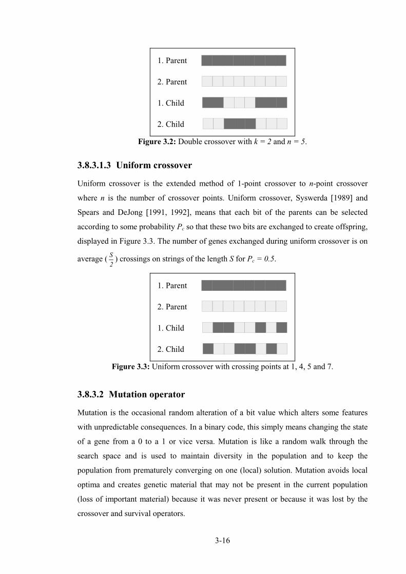
3-16
1. Parent
2. Parent
1. Child
2. Child
Figure 3.2: Double crossover with k = 2 and n = 5.
3.8.3.1.3 Uniform crossover
Uniform crossover is the extended method of 1-point crossover to n-point crossover
where n is the number of crossover points. Uniform crossover, Syswerda [1989] and
Spears and DeJong [1991, 1992], means that each bit of the parents can be selected
according to some probability Pc so that these two bits are exchanged to create offspring,
displayed in Figure 3.3. The number of genes exchanged during uniform crossover is on
average ( S2) crossings on strings of the length S for Pc = 0.5.
1. Parent
2. Parent
1. Child
2. Child
Figure 3.3: Uniform crossover with crossing points at 1, 4, 5 and 7.
3.8.3.2 Mutation operator
Mutation is the occasional random alteration of a bit value which alters some features
with unpredictable consequences. In a binary code, this simply means changing the state
of a gene from a 0 to a 1 or vice versa. Mutation is like a random walk through the
search space and is used to maintain diversity in the population and to keep the
population from prematurely converging on one (local) solution. Mutation avoids local
optima and creates genetic material that may not be present in the current population
(loss of important material) because it was never present or because it was lost by the
crossover and survival operators.
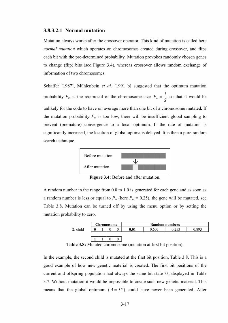
3-17
3.8.3.2.1 Normal mutation
Mutation always works after the crossover operator. This kind of mutation is called here
normal mutation which operates on chromosomes created during crossover, and flips
each bit with the pre-determined probability. Mutation provokes randomly chosen genes
to change (flip) bits (see Figure 3.4), whereas crossover allows random exchange of
information of two chromosomes.
Schaffer [1987], Mühlenbein et al. [1991 b] suggested that the optimum mutation
probability Pm is the reciprocal of the chromosome size PSm = 1
so that it would be
unlikely for the code to have on average more than one bit of a chromosome mutated. If
the mutation probability Pm is too low, there will be insufficient global sampling to
prevent (premature) convergence to a local optimum. If the rate of mutation is
significantly increased, the location of global optima is delayed. It is then a pure random
search technique.
After mutation
Before mutation
Figure 3.4: Before and after mutation.
A random number in the range from 0.0 to 1.0 is generated for each gene and as soon as
a random number is less or equal to Pm (here Pm = 0.25), the gene will be mutated, see
Table 3.8. Mutation can be turned off by using the menu option or by setting the
mutation probability to zero.
Table 3.8:Mutated chromosome (mutation at first bit position).
In the example, the second child is mutated at the first bit position, Table 3.8. This is a
good example of how new genetic material is created. The first bit positions of the
current and offspring population had always the same bit state '0', displayed in Table
3.7. Without mutation it would be impossible to create such new genetic material. This
means that the global optimum ( A = 15 ) could have never been generated. After
Chromosome Random numbers2. child 0 1 0 0 0.01 0.607 0.253 0.893
1 1 0 0
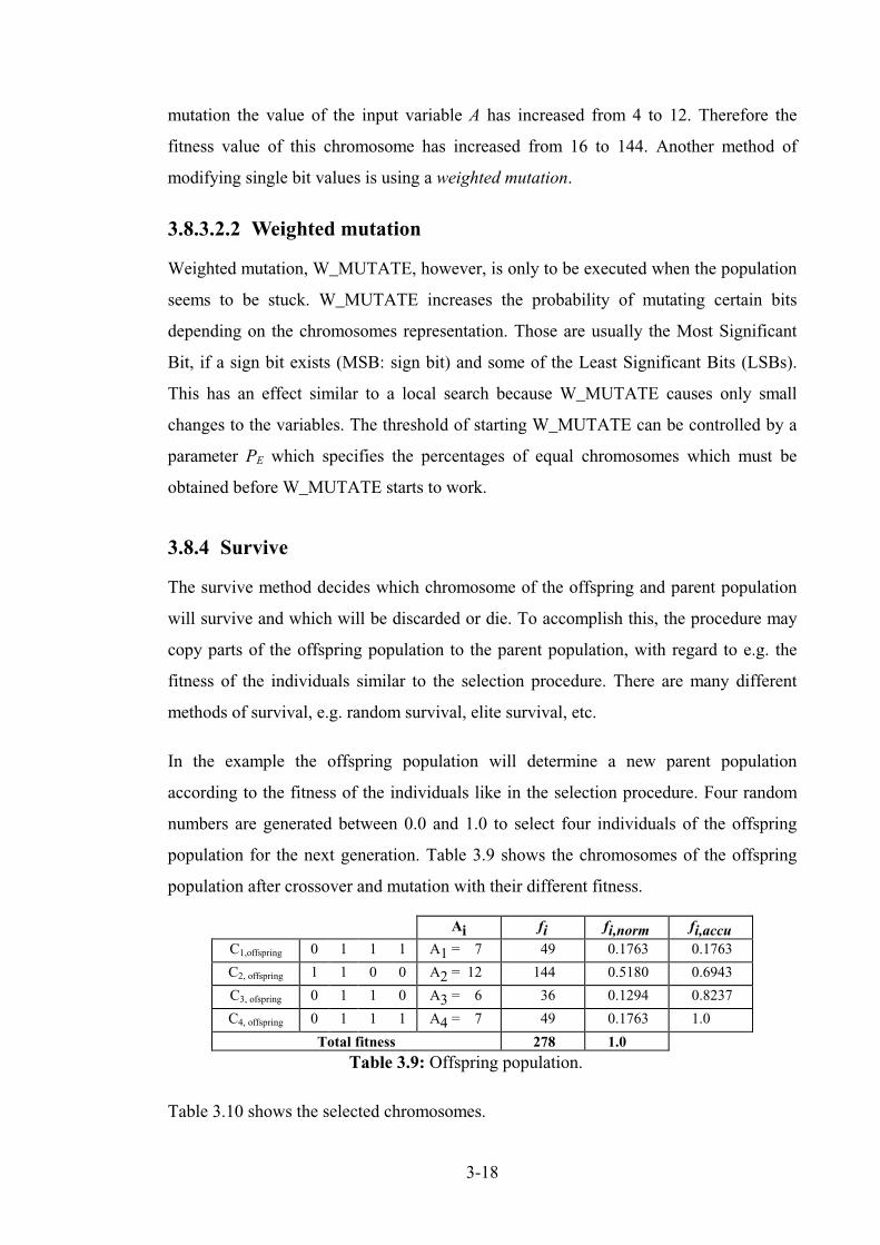
3-18
mutation the value of the input variable A has increased from 4 to 12. Therefore the
fitness value of this chromosome has increased from 16 to 144. Another method of
modifying single bit values is using a weighted mutation.
3.8.3.2.2 Weighted mutation
Weighted mutation, W_MUTATE, however, is only to be executed when the population
seems to be stuck. W_MUTATE increases the probability of mutating certain bits
depending on the chromosomes representation. Those are usually the Most Significant
Bit, if a sign bit exists (MSB: sign bit) and some of the Least Significant Bits (LSBs).
This has an effect similar to a local search because W_MUTATE causes only small
changes to the variables. The threshold of starting W_MUTATE can be controlled by a
parameter PE which specifies the percentages of equal chromosomes which must be
obtained before W_MUTATE starts to work.
3.8.4 Survive
The survive method decides which chromosome of the offspring and parent population
will survive and which will be discarded or die. To accomplish this, the procedure may
copy parts of the offspring population to the parent population, with regard to e.g. the
fitness of the individuals similar to the selection procedure. There are many different
methods of survival, e.g. random survival, elite survival, etc.
In the example the offspring population will determine a new parent population
according to the fitness of the individuals like in the selection procedure. Four random
numbers are generated between 0.0 and 1.0 to select four individuals of the offspring
population for the next generation. Table 3.9 shows the chromosomes of the offspring
population after crossover and mutation with their different fitness.
Table 3.9: Offspring population.
Table 3.10 shows the selected chromosomes.
Ai fi fi,norm fi,accuC1,offspring 0 1 1 1 A1 = 7 49 0.1763 0.1763
C2, offspring 1 1 0 0 A2 = 12 144 0.5180 0.6943
C3, ofspring 0 1 1 0 A3 = 6 36 0.1294 0.8237
C4, offspring 0 1 1 1 A4 = 7 49 0.1763 1.0
Total fitness 278 1.0
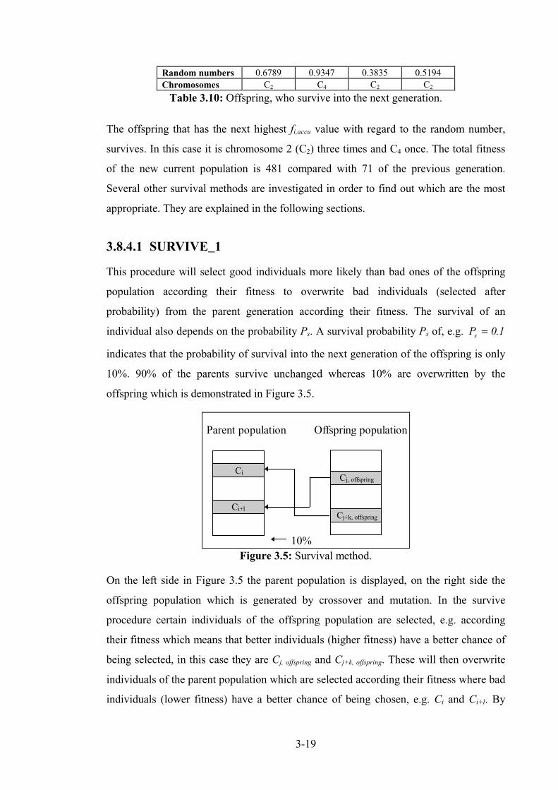
3-19
Table 3.10: Offspring, who survive into the next generation.
The offspring that has the next highest fi,accu value with regard to the random number,
survives. In this case it is chromosome 2 (C2) three times and C4 once. The total fitness
of the new current population is 481 compared with 71 of the previous generation.
Several other survival methods are investigated in order to find out which are the most
appropriate. They are explained in the following sections.
3.8.4.1 SURVIVE_1
This procedure will select good individuals more likely than bad ones of the offspring
population according their fitness to overwrite bad individuals (selected after
probability) from the parent generation according their fitness. The survival of an
individual also depends on the probability Ps. A survival probability Ps of, e.g. Ps = 0 1.
indicates that the probability of survival into the next generation of the offspring is only
10%. 90% of the parents survive unchanged whereas 10% are overwritten by the
offspring which is demonstrated in Figure 3.5.
Ci
Cj+k, offspring
Cj, offspring
Ci+l
Parent population Offspring population
10%Figure 3.5: Survival method.
On the left side in Figure 3.5 the parent population is displayed, on the right side the
offspring population which is generated by crossover and mutation. In the survive
procedure certain individuals of the offspring population are selected, e.g. according
their fitness which means that better individuals (higher fitness) have a better chance of
being selected, in this case they are Cj, offspring and Cj+k, offspring. These will then overwrite
individuals of the parent population which are selected according their fitness where bad
individuals (lower fitness) have a better chance of being chosen, e.g. Ci and Ci+l. By
Random numbers 0.6789 0.9347 0.3835 0.5194Chromosomes C2 C4 C2 C2
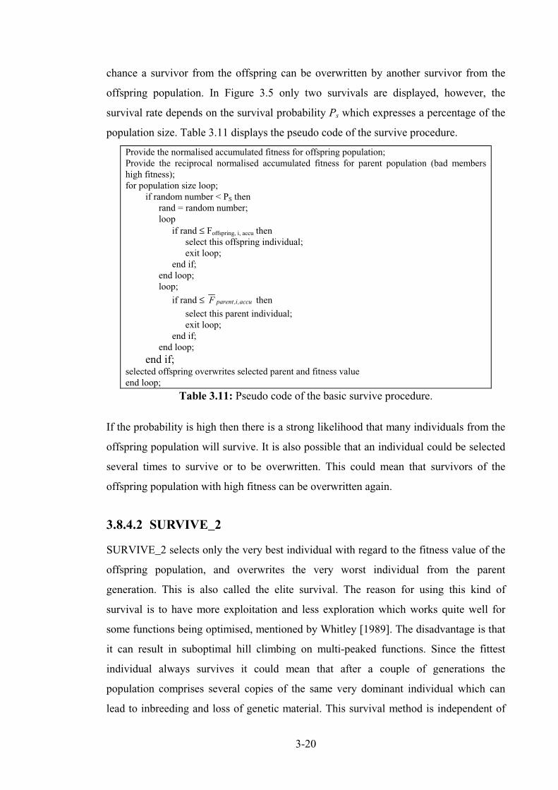
3-20
chance a survivor from the offspring can be overwritten by another survivor from the
offspring population. In Figure 3.5 only two survivals are displayed, however, the
survival rate depends on the survival probability Ps which expresses a percentage of the
population size. Table 3.11 displays the pseudo code of the survive procedure.
Table 3.11: Pseudo code of the basic survive procedure.
If the probability is high then there is a strong likelihood that many individuals from the
offspring population will survive. It is also possible that an individual could be selected
several times to survive or to be overwritten. This could mean that survivors of the
offspring population with high fitness can be overwritten again.
3.8.4.2 SURVIVE_2
SURVIVE_2 selects only the very best individual with regard to the fitness value of the
offspring population, and overwrites the very worst individual from the parent
generation. This is also called the elite survival. The reason for using this kind of
survival is to have more exploitation and less exploration which works quite well for
some functions being optimised, mentioned by Whitley [1989]. The disadvantage is that
it can result in suboptimal hill climbing on multi-peaked functions. Since the fittest
individual always survives it could mean that after a couple of generations the
population comprises several copies of the same very dominant individual which can
lead to inbreeding and loss of genetic material. This survival method is independent of
Provide the normalised accumulated fitness for offspring population;Provide the reciprocal normalised accumulated fitness for parent population (bad membershigh fitness);for population size loop;
if random number < PS thenrand = random number;loop
if rand ≤ Foffspring, i, accu thenselect this offspring individual;exit loop;
end if;end loop;loop;
if rand ≤ F parent i accu, , then
select this parent individual;exit loop;
end if;end loop;
end if;selected offspring overwrites selected parent and fitness valueend loop;

3-21
the survival probability Ps because only the best individual will survive.
3.8.4.3 SURVIVE_3
This procedure is similar to SURVIVE_1. The only difference is that an individual from
the offspring population can only be selected once. A chromosome of the parent
population can only be overwritten once. The survival probability should be less than in
the SURVIVE_1 procedure because otherwise too many low fitness chromosomes will
survive.
3.8.4.4 SURVIVE_4
SURVIVE_4 is similar to the SURVIVE_3 procedure. The only difference is that an
individual of the offspring population can be selected more than once, with regard to its
fitness value, but an individual can only be chosen once from the parent generation to be
overwritten. The advantage of this procedure is that no survivors will be overwritten
again. However, the first offspring to survive, will have been chosen via the elite method
like the SURVIVE_2 procedure. An additional condition is that the fitness value of the
offspring must be at least equal to or better than the fitness value of the selected
individual from the parent generation in order to survive and to overwrite it. If this is not
the case the offspring will be not copied into the parent generation. This has an effect on
the number of survivals which will be less than Ps because not all selected offspring
individuals have a higher fitness than the selected individuals from the parent population
so that these will not survive.
3.8.4.5 SURVIVE_5
SURVIVE_5 is similar to SURVIVE_4 but without the stipulation that the offspring
must be equal to or better than the selected individual of the parent generation. This
should prevent a too strong converging process as might happen in SURVIVE_4,
because stronger diversity is guaranteed. Several experiments have been conducted
using these survive procedures, which are described in chapter 5.
3.9 Why Do GAs work?
GAs search for similarities at certain bit positions, which are also called building blocks
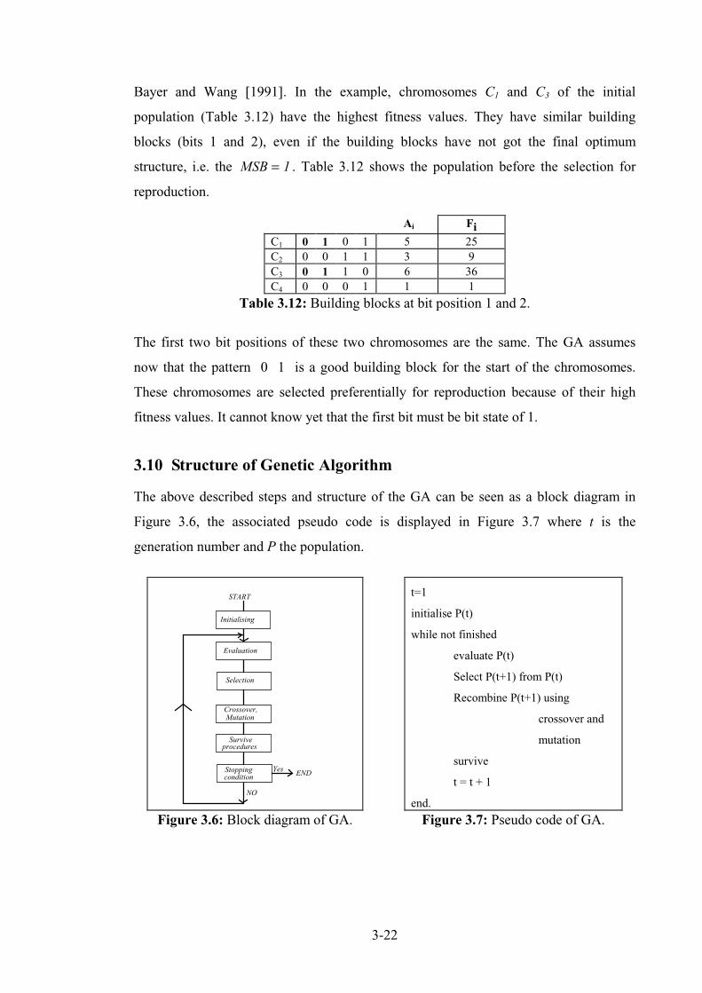
3-22
Bayer and Wang [1991]. In the example, chromosomes C1 and C3 of the initial
population (Table 3.12) have the highest fitness values. They have similar building
blocks (bits 1 and 2), even if the building blocks have not got the final optimum
structure, i.e. the MSB = 1 . Table 3.12 shows the population before the selection for
reproduction.
Table 3.12: Building blocks at bit position 1 and 2.
The first two bit positions of these two chromosomes are the same. The GA assumes
now that the pattern 0 1 is a good building block for the start of the chromosomes.
These chromosomes are selected preferentially for reproduction because of their high
fitness values. It cannot know yet that the first bit must be bit state of 1.
3.10 Structure of Genetic Algorithm
The above described steps and structure of the GA can be seen as a block diagram in
Figure 3.6, the associated pseudo code is displayed in Figure 3.7 where t is the
generation number and P the population.
Ai FiC1 0 1 0 1 5 25C2 0 0 1 1 3 9C3 0 1 1 0 6 36C4 0 0 0 1 1 1
Evaluation
Initialising
Selection
Crossover,Mutation
Surviveprocedures
Stoppingcondition
Yes END
NO
START t=1
initialise P(t)
while not finished
evaluate P(t)
Select P(t+1) from P(t)
Recombine P(t+1) using
crossover and
mutation
survive
t = t + 1
end.
Figure 3.6: Block diagram of GA. Figure 3.7: Pseudo code of GA.
3-23
3.11 Performance
Although the goal is clearly to achieve an optimum solution, It is undesirable that the
entire population should converge to the same value. This is because valuable
information which is developed in part of the population is often lost. Therefore, the
population needs to be diverse, so that a wide search of the input domain is guaranteed.
If the population converges prematurely or too fast, the penalty will be to lose
information which restricts the exploration of the search space. DeJong [1975] defined a
converged allele, when a particular gene has at least 95% of all individuals the same
value in a population. Since the characteristics of the function which is to be optimised,
are unknown, such a restriction may prevent the finding of the optimum solution. Baker
[1985] mentioned three metrics for the performance of genetic algorithms which were
proposed by Grefenstette [1986]. They are:
1. The on-line performance is the average fitness value of all individuals that have been
generated and evaluated. It penalises those search methods which have to test many
poor solutions (structures) before generating a solution for the global optimum. In
order to have a high on-line performance the GA has to concentrate on those areas in
the search space where the best values lie.
2. The off-line performance is the average of the best individual fitness from each
generation. This method will not penalise exploring poor regions of the search space
which may lead to better solutions.
3. The best individual is the individual with the highest fitness that has been generated.
If the diversity is increased, the on-line performance measure will be affected quite
badly. A restricted convergence impairs the off-line performance. A usual reason for fast
convergence is the existence of a very fit (super) individual that dominates the
population surviving many more times and hence reducing the variety of genetic
material available. In a small number of generations the super individual and its
descendants can dominate the entire population. To avoid this phenomenon Baker places
a threshold on an individual’s expected number of offspring.
3.12 Exploiting the power of genetic algorithms
The key feature of GAs is their capability to exploit information gathered about an
3-24
initially unknown search space. This directs other searches into useful sub-spaces. If the
space of legal structural changes is not too large, an enumerative search strategy can be
developed with appropriate heuristic cut-offs in order to keep the computation time
under control. However, if the search space is large, much time and effort can be spent
in developing domain knowledge heuristics. It is exactly in these occasions (large,
extremely non-linear, complex, poorly understood search spaces) where the GAs have
been used successfully. Even for large search spaces (e.g. 1030 points), DeJong [1988]
mentioned that suitable combinations are found after only a couple of simulated
generations.
3.12.1 The role of feedback
So far a description of how GAs work and how their power can be exploited has been
given. In this section the focus is on one of the issues in the optimisation process - the
role of feedback.
GAs can be used as an adaptive sampling strategy to search large and complex spaces.
This sampling strategy is adaptive with regard to feedback from the samples (offspring)
being used to bias subsequent sampling into regions with high expected performance
(global optimum). This means that, even if a good solution has been generated, the
effectiveness of GAs in optimising parameters also depends on the usefulness of the
information obtained via the feedback. It is important that the right feedback mechanism
is selected to enable an adaptive search strategy.
Such feedback mechanisms have been shown to be very effective, Schaffer [1985] and
DeJong [1988]. Feedback mechanisms are called fitness, cost or pay-off functions. This
form of feedback uses a reward and punishment method, in which performance
evaluation is stated in terms of a fitness function. GAs can employ this information
directly, to influence the selection of parents who will be used to produce new offspring
or for the survival of the offspring. Not all fitness functions are equally suited. A good
function will provide useful information early in the search process to help focus
attention. For example, a fitness function that almost always gives zero fitness, provides
almost no information for directing the search process. Therefore suitable fitness
functions must be found which describe the environment of the problem in order to
exploit the search space and therefore the power of the GA.
3-25
3.12.2 The use of domain knowledge
GAs are normally categorised as domain-independent search and optimisation methods
so that they can be applied without any knowledge of the space being searched.
However, although no domain knowledge is required, there are possibilities and
opportunities to incorporate domain knowledge. A good example of domain knowledge
involves the choice of the initial population, which is described earlier as randomly
selected, but there is no reason not to use available information that permits seeding the
initial population with individuals who have a certain knowledge about the problem and
which may be close to a global solution.
Another obvious method to exploit domain knowledge is by means of the feedback
mechanism. As described earlier, the effectiveness of the GAs relies on the usefulness of
the feedback information (fitness function) provided.
3.13 Interim conclusion
As the example in this chapter shows, the obvious desire is to achieve an optimum
solution for a particular function. How a GA works is shown with a simple problem.
The main characteristics of GAs are listed below:
1. Concentrates on chromosomes with above average fitness.
2. Exploits information about a large number of values while processing a small
population.
3. Prevents search from stagnating at a local optimum.
4. They take advantage of old knowledge held in a population of solutions to generate
new solutions with improved performance.
In the case that a fitness-proportional selection procedure is the only active part of a
optimisation, an initial random generated population of size N will quite rapidly create a
population which will only contain N duplicates of the best individual (highest fitness).
The GAs counterbalance this selective pressure by the genetic operator (crossover and
mutation) toward a uniformity by generating diversity in the form of new alleles and
their combination. GAs rapidly locate the area in which a global optimum could be
found, but need much more time to pinpoint it, DeJong [1993].

3-26
In the next chapter, the approach of software testing is described. The method covers the
testing of 'if' conditions, various loops and different data types.

4-1
CHAPTER 4
A strategy for applying GAs and random numbers to
software testing
GAs form a method of adaptive search in the sense that they modify the test data from
one generation to the next, in order to optimise a fitness function. In contrast random
testing generates test data without using any knowledge of previous test data.
This chapter describes the interface between the software under test and testing tool
which uses either the GA or random numbers. The method random numbers is used as a
comparison of the GA testing strategy.
4.1 Testing using Random Testing
In order to measure the effectiveness of GA testing, random testing is carried out. The
random generation of tests identifies members of the subdomains arbitrarily, with a
homogeneous probability which is related to the cardinality of the subdomains. Under
these circumstances, the chances of testing a function, whose subdomain has a low
cardinality with regard to the domain as a whole, is much reduced. A pseudo random
number generator generates the test data with no use of feedback from previous tests.
The tests are passed to the procedure under test, in the hope that all branches will be
traversed. Watt's [1987] pseudo random number generator, written in Ada, has been
used and tested and has a uniform distribution. The test harness used for random testing
is the same as that used for GAs. The only difference is the way data is generated.
4.2 Subdomains
A search space is defined and the GAs and random numbers probe for the global
optimum (goal). In this case the search space is the domain D of input variables xi for the
software under test, and is given by the set D = {x1, x2 , ..., xm}. The domain D may be
split into a group of subdomains, di, displayed in Figure 2.2.
Each path through the program identifies a unique subdomain. The conditions and
statements in a software program partitions the input space into a set of exclusive

4-2
domains. Each of these subdomains belongs to a certain software path and identifies a
unique function. They consist of input data which will cause a certain path to be
executed. In this case there are only two input variables A and B. The domain is split up
into several subdomains and each of them cause one specific path in the software to be
traversed where early branches in the control flow usually have a higher cardinality than
subsequent branches which tend to be smaller because of the filtering effect of
successive branches.
The goal for the GAs is typically to search for members of these particular subdomains
ds = {xj,...,xk}. One way of generating high adequacy test data is, therefore, to find test
sets which fall at or near the boundaries of a subdomain in order to identify whether the
boundary between subdomains is wrongly located, see Figure 2.2. A test data set is
considered to be a set of values {x1, x2, ..., xm}. Each value corresponds to an input
variable of the procedure to be tested. The problem remains how the boundary of a
subdomain may be identified. This problem may be acute when the subdomains are
multi-dimensioned, disconnected or isolated. The solution of the problem is an example
of partition testing, and it lies in the location of a member of the subdomain boundary,
dsb, which is a proper subset, i.e. d ds
bs⊆ .
4.2.1 Fitness functions adapted from predicates
On the basis of the preceding argument, subdomains of functionality align with the path
structure of the program, and their boundaries may be found by examining the predicates
at different points along the path. A predicate is a Boolean expression involving
functions of the input variables, constants, related variables and relational operators. The
aim of this work is to identify test sets which, when changed by a small amount (where
small is defined in terms of the underlying data type), cause the predicate to switch from
true to false, or vice versa. It is these pivotal values which form the basis of the genetic
algorithm fitness function. By choosing the fitness function to give higher fitness rating
for boundary test sets (closer to boundary), GAs will identify test sets which are more
likely to reveal faults, Clarke [1976]. These test sets are called boundary test data
because they are the next to the boundaries defined by the predicates.
The fitness functions which are used in the next chapters are based on the predicates of
4-3
the software under test, and the system attempts to exercise every branch. A fitness
function is applied to predicates involving the input variables. Each predicate has its
own fitness function in order to evaluate the test data performance. For example, a
predicate function has the form of:
h X rop g X( ) ( ) (4.1)
where X = {x1, x2, ..., xm}
where h and g may be complex functions of the test set ( input variables) {x1, x2, ... , xm}
and rop is one of the relational operator {<, >, ≤, ≥, , =, ≠}. The power of GAs and the
testing tool is that the form of h and g need not be known explicitly, only their values,
which are made available by suitable instrumentation of software at that point where the
predicate is executed. A possible fitness function, F, is the reciprocal of the distance
between the two functions, i.e.
F h X g X n= − + −( ( ) ( ) )δ (4.2)
where n is a positive integer and δ is a small quantity to prevent numericoverflow.
Whatever relational operator is involved, this approach will assign higher fitness
measures to boundary test sets. This function has been adapted to use n = 1, n = 3 or the
Gaussian function. In general, none of these performed better than the inverse square
law (n = 2).
The GAs will be used to generate those data which are close to the boundary in order to
traverse all branches, because the closer the test data are to the boundary, the more
information is provided about the correctness of the condition under test. Another
advantage of boundary test data is that if one of two branches of the same condition has
not been executed, test data closer to boundaries are usually more likely to lead to test
data which crosses the boundary and covers the opposite branch. Each branch will have
a different fitness function with regard to its predicate. Those branches which are
traversed, do not need to be visited so reducing computational time. The system looks
for the next untraversed branch and will concentrate on that node in order to execute it.
The execution of a branch, only once, is appropriate because every test set generated
from the same subdomain will execute the same functions and follow the same branch,

4-4
so that all remaining test sets of that subdomain will work correctly too. Therefore, no
more information is gained by executing more than one test set from the same sub -
domain. The exception is when boundary test data have to be generated to check the
boundary between sub - domains because an error in the boundary can lead to a shifting
of it (using '>' instead of '≥') which can be located with boundary test data.
4.3 Control flow tree and graph
The structure of a program or procedure can be shown by a control flow diagram. The
control flow diagram may be represented as a tree or a graph whose nodes represent
sequences of statements followed by a jump initiated by a selection such as an if -
condition or the condition of a loop. The jump is indicated by the edges of the nodes. A
control flow tree / graph divides a program into nodes and edges. A control flow tree
compared to a graph has no edges back from a later node to a previous node, i.e. it exists
no loop statement. The nodes represent statements in a program, the edges depict the
actions of a program to get from one node to another. The edges express the flow of the
control and they are between each of these statements. The combination of a node and
branch is, therefore, equivalent to the LCSAJ (linear code sequence and jump). A
LCSAJ is defined as a sequence of code where the flow of control is sequential and
terminates by a jump in the control flow. Nodes which have no following nodes are
called leaf nodes.
A structured database equivalent to the control flow tree is created, i.e. information with
regard to the nodes can be stored. This information includes nodes that have been
executed and not been executed, test sets which executed the nodes and fitness values of
the test sets.
A path is defined by White and Cohen [1980], by executing the node with the initial
statement (entry node) and the path terminates with the node of the last statement (exit
node). There must be only one entry node, but there could be several exit nodes.
Two control flows through a program, which differ only in the number of times a
particular loop has been executed, are two distinct paths. Therefore the number of paths
in a program with loops can be infinite because loops may iterate any number of times.
In general path testing is impossible.
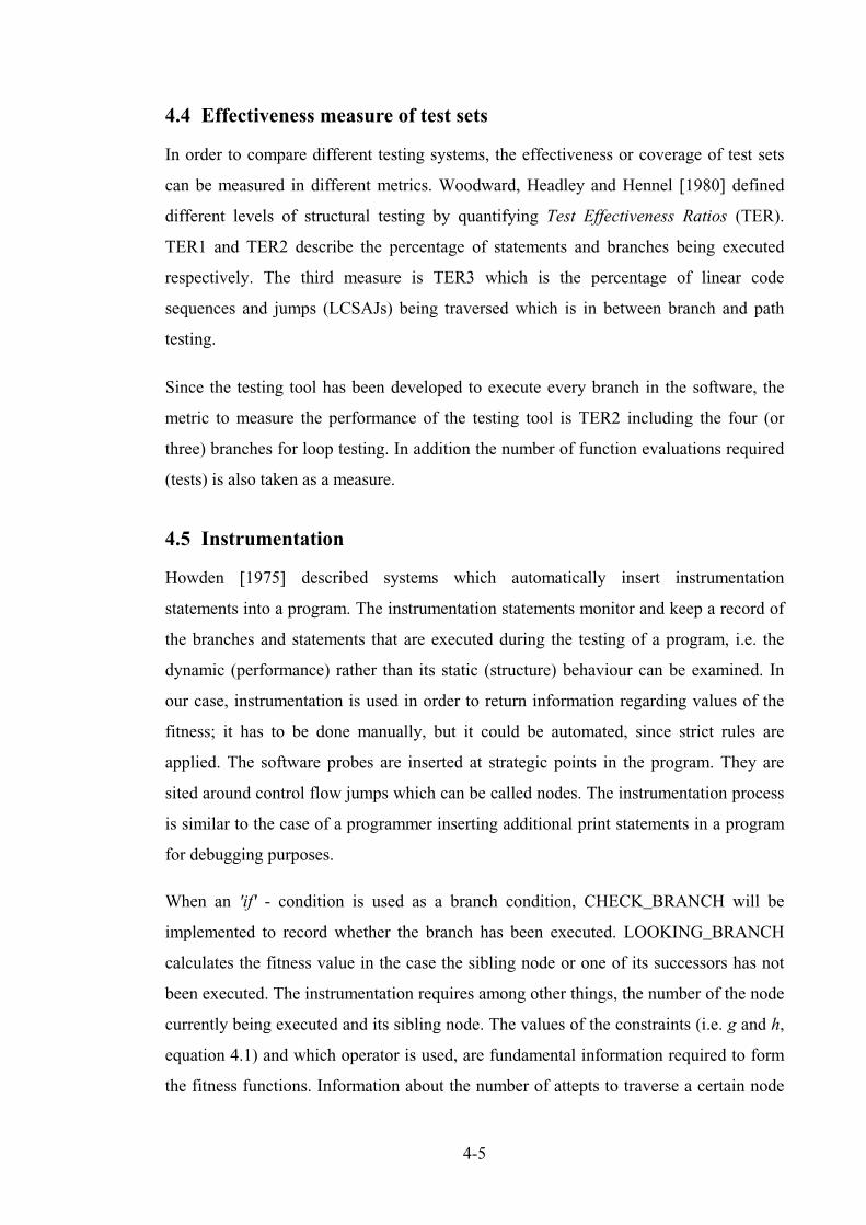
4-5
4.4 Effectiveness measure of test sets
In order to compare different testing systems, the effectiveness or coverage of test sets
can be measured in different metrics. Woodward, Headley and Hennel [1980] defined
different levels of structural testing by quantifying Test Effectiveness Ratios (TER).
TER1 and TER2 describe the percentage of statements and branches being executed
respectively. The third measure is TER3 which is the percentage of linear code
sequences and jumps (LCSAJs) being traversed which is in between branch and path
testing.
Since the testing tool has been developed to execute every branch in the software, the
metric to measure the performance of the testing tool is TER2 including the four (or
three) branches for loop testing. In addition the number of function evaluations required
(tests) is also taken as a measure.
4.5 Instrumentation
Howden [1975] described systems which automatically insert instrumentation
statements into a program. The instrumentation statements monitor and keep a record of
the branches and statements that are executed during the testing of a program, i.e. the
dynamic (performance) rather than its static (structure) behaviour can be examined. In
our case, instrumentation is used in order to return information regarding values of the
fitness; it has to be done manually, but it could be automated, since strict rules are
applied. The software probes are inserted at strategic points in the program. They are
sited around control flow jumps which can be called nodes. The instrumentation process
is similar to the case of a programmer inserting additional print statements in a program
for debugging purposes.
When an 'if' - condition is used as a branch condition, CHECK_BRANCH will be
implemented to record whether the branch has been executed. LOOKING_BRANCH
calculates the fitness value in the case the sibling node or one of its successors has not
been executed. The instrumentation requires among other things, the number of the node
currently being executed and its sibling node. The values of the constraints (i.e. g and h,
equation 4.1) and which operator is used, are fundamental information required to form
the fitness functions. Information about the number of attepts to traverse a certain node
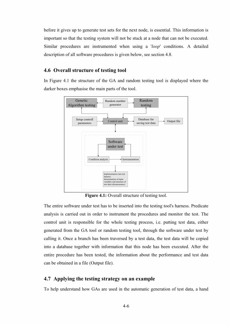
4-6
before it gives up to generate test sets for the next node, is essential. This information is
important so that the testing system will not be stuck at a node that can not be executed.
Similar procedures are instrumented when using a 'loop' conditions. A detailed
description of all software procedures is given below, see section 4.8.
4.6 Overall structure of testing tool
In Figure 4.1 the structure of the GA and random testing tool is displayed where the
darker boxes emphasise the main parts of the tool.
Softwareunder test
Condition analysis Instrumentation
Implementation into testharness;determination of inputvariables and structure oftest data (chromosomes)
Control unit
GeneticAlgorithm testing
Randomtesting
Random numbergenerator
Database forsaving test data
Output fileSetup controllparameters
Figure 4.1: Overall structure of testing tool.
The entire software under test has to be inserted into the testing tool's harness. Predicate
analysis is carried out in order to instrument the procedures and monitor the test. The
control unit is responsible for the whole testing process, i.e. putting test data, either
generated from the GA tool or random testing tool, through the software under test by
calling it. Once a branch has been traversed by a test data, the test data will be copied
into a database together with information that this node has been executed. After the
entire procedure has been tested, the information about the performance and test data
can be obtained in a file (Output file).
4.7 Applying the testing strategy on an example
To help understand how GAs are used in the automatic generation of test data, a hand

4-7
worked example for the control flow tree given in Figure 2.2 (page 2-7) will be
explained. The example is intended to illustrate the general principle of the process and
not its detailed working. The detailed working of the strategy and of the instrumented
procedures are explained in more detail in section 4.8. Figure 4.2 repeats the example
from chapter 2 (Figure 2.2) to remind the reader.
Listing 4.2 displayes the example with the instrumented procedures.
Listing 4.2: Example with instrumentation.
The most important parameter settings for the GA are given in Table 4.1.
Table 4.1: Settings for the GA.
Table 4.2 shows the first generation which is randomly generated by the testing tool.
Each row in the table represents a member of the population whose size is 4. The
columns in Table 4.2 have the following meaning:
• Pi indicates a member of the parent population;
if A ≤≤≤≤ B thenput("node 2");if A = B thenput("node 3");
else --A < Bput("node 4");
end if;else --A > Bput("node 5");
end if;
1
2 5
A = B
A > B
3 4
A < B
A <= B
Figure 4.2: Software and control flow tree for the example.
if A ≤≤≤≤ B thenCHECK_BRANCH(2);LOOKING_BRANCH(5, A, B + 1);if A = B then
CHECK_BRANCH(3);LOOKING_BRANCH(4, A, B - 1);
else --A < BCHECK_BRANCH(4);LOOKING_BRANCH(3, A, B);
end if;else --A > B
CHECK_BRANCH(5);LOOKING_BRANCH(2, A, B);
end if;
Selection of parents for recombination is randomThe mutated genes (bits) are bold in the offspring populationFitness is calculated according reciprocal fitness functionSingle crossoverSurvive probability Ps = 0.5Mutation probability Pm = 0.1

4-8
• A and B are the values of the identifiers representing the input variables;
• look (short for looking) gives the node number to be traversed;
• Path indicates which nodes have been traversed by this current test data of A and B;
• chromosome displays the bit pattern of the test data in binary-plus-sign bit format;
• fitness gives the fitness value calculated according to the test data and the node
required to be traversed;
• fi,norm is the normalised fitness;
• fi,accu is the accumulated normalised fitness value;
• Ft indicates the population total fitness value.
Table 4.2: First generation.
There are two points to note concerning the fields in Table 4.2 which are:
(i) A 5 bit representation per input test data has been chosen. Therefore, the
chromosome size is 10 bits where the first five bits represents the input data A and
the rest the input data B. The least significant bit is stored on the left hand side and
the most significant bit (sign bit) on the right hand side of the two substrings within
the chromosome. This representation conforms to the conversion function that is
provided by Ada.
(ii) A large fi,norm value indicates that these population members have a high fitness and
hence have a higher probability of surviving into the next generation.
The first test data (P1) is put into the software under test. The first node required to be
executed is node 2 (see look in first generation).
The fitness function f, which calculates the test data performance and is based on the
conditions in the code (see chapter 3.8.1) is for this node fA B
=− +
1
0 01 2( . )because
the boundary test data to traverse the condition A B≤ (node 2) is A = B. The test sets in
the first generation execute nodes 1, 2, 4, and 5 leaving only node 3 untraversed. This
fitness function ensures that test data where A and B are numerical close to each other
Pi A B look Path chromosome fitness fi,norm fi,accuP1 4 10 2 1, 2, 4 00100 01010 0.0278 0.365 0.365P2 -7 -15 2 1,5 11101 11111 0.0156 0.205 0.570P3 8 15 2 1, 2, 4 00010 11110 0.0204 0.268 0.838P4 3 -6 2 1, 5 11000 01101 0.0123 0.162 1.0 Ft = 0.076
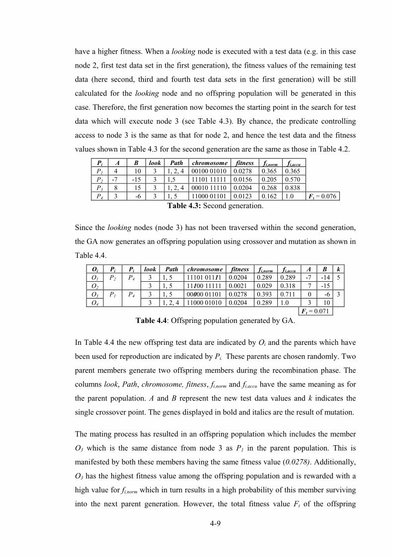
4-9
have a higher fitness. When a looking node is executed with a test data (e.g. in this case
node 2, first test data set in the first generation), the fitness values of the remaining test
data (here second, third and fourth test data sets in the first generation) will be still
calculated for the looking node and no offspring population will be generated in this
case. Therefore, the first generation now becomes the starting point in the search for test
data which will execute node 3 (see Table 4.3). By chance, the predicate controlling
access to node 3 is the same as that for node 2, and hence the test data and the fitness
values shown in Table 4.3 for the second generation are the same as those in Table 4.2.
Table 4.3: Second generation.
Since the looking nodes (node 3) has not been traversed within the second generation,
the GA now generates an offspring population using crossover and mutation as shown in
Table 4.4.
Table 4.4: Offspring population generated by GA.
In Table 4.4 the new offspring test data are indicated by Oi and the parents which have
been used for reproduction are indicated by Pi. These parents are chosen randomly. Two
parent members generate two offspring members during the recombination phase. The
columns look, Path, chromosome, fitness, fi,norm and fi,accu have the same meaning as for
the parent population. A and B represent the new test data values and k indicates the
single crossover point. The genes displayed in bold and italics are the result of mutation.
The mating process has resulted in an offspring population which includes the member
O3 which is the same distance from node 3 as P1 in the parent population. This is
manifested by both these members having the same fitness value (0.0278). Additionally,
O3 has the highest fitness value among the offspring population and is rewarded with a
high value for fi,norm which in turn results in a high probability of this member surviving
into the next parent generation. However, the total fitness value Ft of the offspring
Pi A B look Path chromosome fitness fi,norm fi,accuP1 4 10 3 1, 2, 4 00100 01010 0.0278 0.365 0.365P2 -7 -15 3 1,5 11101 11111 0.0156 0.205 0.570P3 8 15 3 1, 2, 4 00010 11110 0.0204 0.268 0.838P4 3 -6 3 1, 5 11000 01101 0.0123 0.162 1.0 Ft = 0.076
Oi Pi Pi look Path chromosome fitness fi,norm fi,accu A B kO1 P2 P4 3 1, 5 11101 01111 0.0204 0.289 0.289 -7 -14 5O2 3 1, 5 11100 11111 0.0021 0.029 0.318 7 -15O3 P1 P4 3 1, 5 00000 01101 0.0278 0.393 0.711 0 -6 3O4 3 1, 2, 4 11000 01010 0.0204 0.289 1.0 3 10
Ft = 0.071
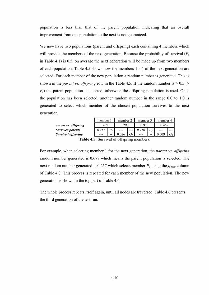
4-10
population is less than that of the parent population indicating that an overall
improvement from one population to the next is not guaranteed.
We now have two populations (parent and offspring) each containing 4 members which
will provide the members of the next generation. Because the probability of survival (Ps
in Table 4.1) is 0.5, on average the next generation will be made up from two members
of each population. Table 4.5 shows how the members 1 - 4 of the next generation are
selected. For each member of the new population a random number is generated. This is
shown in the parent vs. offspring row in the Table 4.5. If the random number is > 0.5 (>
Ps) the parent population is selected, otherwise the offspring population is used. Once
the population has been selected, another random number in the range 0.0 to 1.0 is
generated to select which member of the chosen population survives to the next
generation.
Table 4.5: Survival of offspring members.
For example, when selecting member 1 for the next generation, the parent vs. offspring
random number generated is 0.678 which means the parent population is selected. The
next random number generated is 0.257 which selects member P1 using the fi,accu column
of Table 4.3. This process is repeated for each member of the new population. The new
generation is shown in the top part of Table 4.6.
The whole process repeats itself again, until all nodes are traversed. Table 4.6 presents
the third generation of the test run.
member 1 member 2 member 3 member 4parent vs. offspring 0.678 0.298 0.978 0.457Survived parents 0.257 P1 --- --- 0.710 P3 --- ---Survived offspring --- -- 0.026 O1 --- -- 0.609 O3
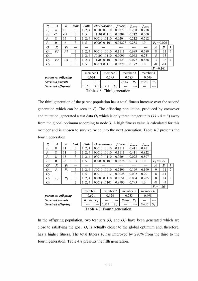
4-11
Table 4.6: Third generation.
The third generation of the parent population has a total fitness increase over the second
generation which can be seen in Ft. The offspring population, produced by crossover
and mutation, generated a test data O1 which is only three integer units (11 - 8 = 3) away
from the global optimum according to node 3. A high fitness value is calculated for this
member and is chosen to survive twice into the next generation. Table 4.7 presents the
fourth generation.
Table 4.7: Fourth generation.
In the offspring population, two test sets (O1 and O4) have been generated which are
close to satisfying the goal. O4 is actually closer to the global optimum and, therefore,
has a higher fitness. The total fitness Ft has improved by 280% from the third to the
fourth generation. Table 4.8 presents the fifth generation.
Pi A B look Path chromosome fitness fi,norm fi,accuP1 4 10 3 1, 2, 4 00100 01010 0.0277 0.288 0.288P2 -7 -14 3 1, 5 11101 01111 0.0204 0.212 0.500P3 8 15 3 1, 2, 4 00010 11110 0.0204 0.212 0.712P4 0 -6 3 1, 5 00000 01101 0.02278 0.288 1.0 Ft = 0.096Oi Pi Pi --- --- --- --- --- --- A B kO1 P3 P1 3 1, 2, 4 00010 11010 0.1111 0.689 0.689 8 11 7O2 3 1, 2, 4 10100 11110 0.0099 0.062 0.751 5 15O3 P2 P4 3 1, 2, 4 11000 01101 0.0123 0.077 0.828 3 -6 4O4 3 1, 5 00011 01111 0.0278 0.172 1.0 -8 -14
Ft =0.161member 1 member 2 member 3 member 4
parent vs. offspring 0.034 0.295 0.785 0.546Survived parents --- --- --- --- 0.540 P3 0.952 P4
Survived offspring 0.158 O1 0.331 O1 --- --- --- ---
Pi A B look Path chromosome fitness fi,norm fi,accuP1 8 11 3 1, 2, 4 00010 11010 0.1111 0.411 0.411P2 8 11 3 1, 2, 4 00010 11010 0.1111 0.411 0.822P3 8 15 3 1, 2, 4 00010 11110 0.0204 0.075 0.897P4 0 -6 3 1, 5 00000 01101 0.0278 0.103 1.0 Ft = 0.27Oi Pi Pi --- --- --- --- --- --- A B kO1 P1 P2 3 1, 2, 4 10010 11010 0.2499 0.199 0.199 9 11 2O2 3 1, 5 00010 11011 0.0028 0.002 0.201 8 -11O3 P4 P3 3 1, 2, 4 00000 01110 0.0051 0.004 0.205 0 14 8O4 3 1, 2, 4 00011 11101 0.9990 0.795 1.0 -8 -7
Ft = 1,26member 1 member 2 member 3 member 4
parent vs. offspring 0.691 0.124 0.753 0.498Survived parents 0.356 P1 --- --- 0.861 P3 --- ---Survived offspring --- --- 0.551 O4 --- --- 0.050 O1
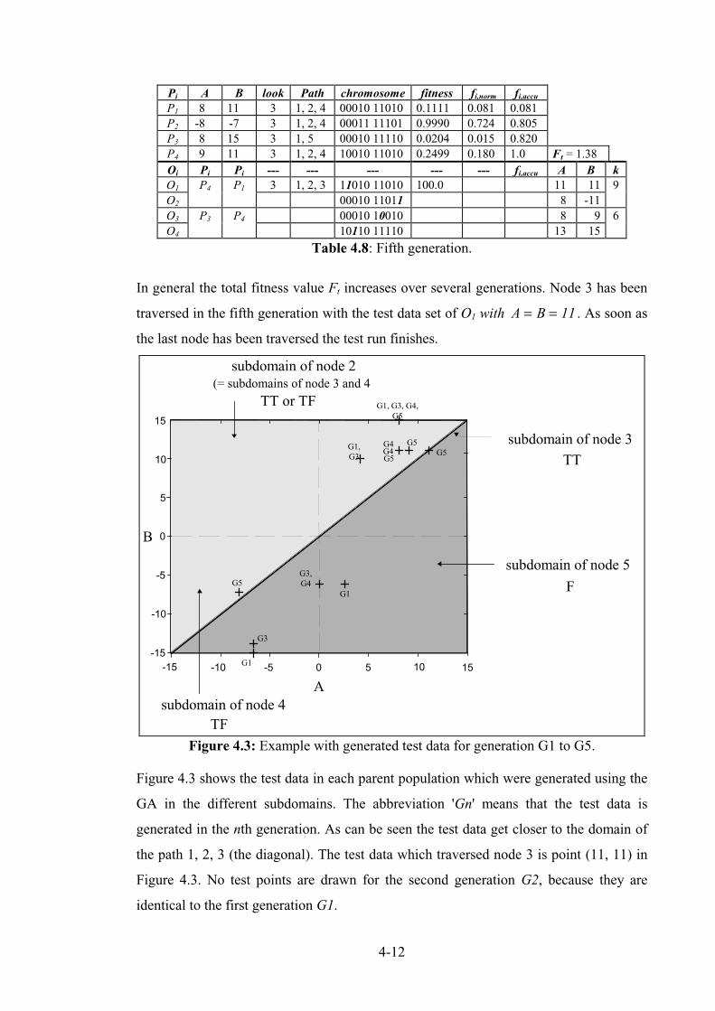
4-12
Table 4.8: Fifth generation.
In general the total fitness value Ft increases over several generations. Node 3 has been
traversed in the fifth generation with the test data set of O1 with A B= = 11 . As soon as
the last node has been traversed the test run finishes.
-15 -10 -5 0 5 10 15-15
-10
-5
0
5
10
15
A
B
subdomain of node 4TF
subdomain of node 5
F
subdomain of node 3TT
subdomain of node 2
TT or TF(= subdomains of node 3 and 4
G1,G3
G1
G1, G3, G4,G5
G1
G3,G4
G3
G4G4
G5
G5
G5G5
Figure 4.3: Example with generated test data for generation G1 to G5.
Figure 4.3 shows the test data in each parent population which were generated using the
GA in the different subdomains. The abbreviation 'Gn' means that the test data is
generated in the nth generation. As can be seen the test data get closer to the domain of
the path 1, 2, 3 (the diagonal). The test data which traversed node 3 is point (11, 11) in
Figure 4.3. No test points are drawn for the second generation G2, because they are
identical to the first generation G1.
Pi A B look Path chromosome fitness fi,norm fi,accuP1 8 11 3 1, 2, 4 00010 11010 0.1111 0.081 0.081P2 -8 -7 3 1, 2, 4 00011 11101 0.9990 0.724 0.805P3 8 15 3 1, 5 00010 11110 0.0204 0.015 0.820P4 9 11 3 1, 2, 4 10010 11010 0.2499 0.180 1.0 Ft = 1.38Oi Pi Pi --- --- --- --- --- fi,accu A B kO1 P4 P1 3 1, 2, 3 11010 11010 100.0 11 11 9O2 00010 11011 8 -11O3 P3 P4 00010 10010 8 9 6O4 10110 11110 13 15

4-13
4.8 Method of testing
In this section the test strategy is explained in more detail with examples for ie. 'if'
conditions and loop statements. The task of the instrumented procedures are described
and the method of generating boundary test data are outlined.
4.8.1 Testing 'if ... then ... else' conditions
Figure 4.4: Control flow tree of an 'if...then....else' condition and the correspondingoriginal software.
Figure 4.4 shows an example of the control tree of a simple 'if ... then ... else' condition
and the software before the instrumentation. CN represents a predicate function
(described in equation 4.1), SN+1 (corresponding to node (N+1)) and SN+2 (corresponding
to node (N+2)) are different sequences of statements to be executed. SN+1 is executed if
CN is true otherwise SN+2 is executed. Suppose the condition CN denotes A B= (see
example in Figure 2.2, using the condition of node 2) where A and B are unknown
integer identifiers and may be complicated functions of the input parameters {x1, x2,
...,xm}. To traverse SN+1 in node (N+1), A must have a value of B. A may have any value
not equal to B ( A B≠ ) to execute SN+2 in node (N+2). A preferable value for A is B ± 1
since it is next to the subdomain boundary and, therefore, more likely to reveal errors
than any other values for A. In terms of GAs this means that the closer the value of A is
to B for node (N+1), the higher the fitness should be. Unfortunately these subdomain
boundary values are quite often difficult to generate. In order to know which node has
already been executed, the program under test is controlled by a test harness, and has to
be instrumented. All necessary input parameters {x1, x2, ...,xm} are stored in a record
containing the input parameters. Figure 4.5 shows the kind of instrumentation that takes
place for the code segment shown in Figure 4.4.
N
N+1 N+2
elseif C thenN
if CN thenSN+1
elseSN+2
end if;
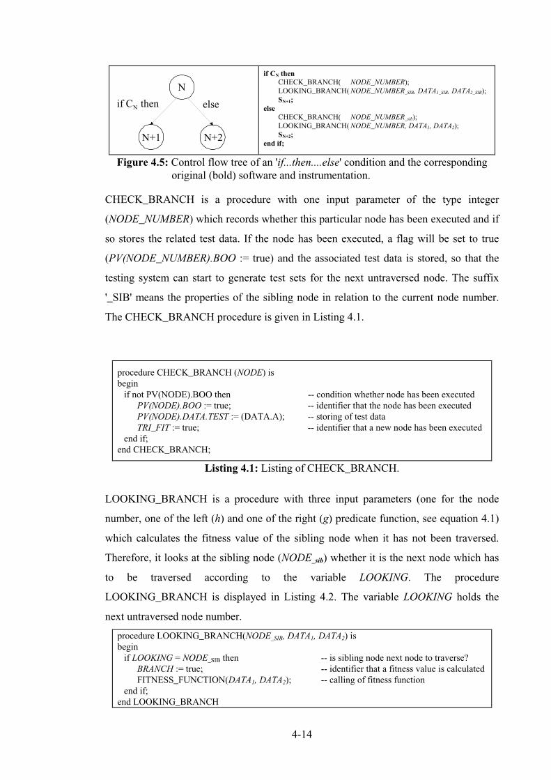
4-14
Figure 4.5: Control flow tree of an 'if...then....else' condition and the correspondingoriginal (bold) software and instrumentation.
CHECK_BRANCH is a procedure with one input parameter of the type integer
(NODE_NUMBER) which records whether this particular node has been executed and if
so stores the related test data. If the node has been executed, a flag will be set to true
(PV(NODE_NUMBER).BOO := true) and the associated test data is stored, so that the
testing system can start to generate test sets for the next untraversed node. The suffix
'_SIB' means the properties of the sibling node in relation to the current node number.
The CHECK_BRANCH procedure is given in Listing 4.1.
Listing 4.1: Listing of CHECK_BRANCH.
LOOKING_BRANCH is a procedure with three input parameters (one for the node
number, one of the left (h) and one of the right (g) predicate function, see equation 4.1)
which calculates the fitness value of the sibling node when it has not been traversed.
Therefore, it looks at the sibling node (NODE_sib) whether it is the next node which has
to be traversed according to the variable LOOKING. The procedure
LOOKING_BRANCH is displayed in Listing 4.2. The variable LOOKING holds the
next untraversed node number.
N
N+1 N+2
elseif C thenN
if CN thenCHECK_BRANCH( NODE_NUMBER);LOOKING_BRANCH(NODE_NUMBER_SIB, DATA1_SIB, DATA2_SIB);SN+1;
elseCHECK_BRANCH( NODE_NUMBER_sib);LOOKING_BRANCH(NODE_NUMBER, DATA1, DATA2);SN+2;
end if;
procedure CHECK_BRANCH (NODE) isbeginif not PV(NODE).BOO then -- condition whether node has been executed
PV(NODE).BOO := true; -- identifier that the node has been executedPV(NODE).DATA.TEST := (DATA.A); -- storing of test dataTRI_FIT := true; -- identifier that a new node has been executed
end if;end CHECK_BRANCH;
procedure LOOKING_BRANCH(NODE_SIB, DATA1, DATA2) isbeginif LOOKING = NODE_SIB then -- is sibling node next node to traverse?
BRANCH := true; -- identifier that a fitness value is calculatedFITNESS_FUNCTION(DATA1, DATA2); -- calling of fitness function
end if;end LOOKING_BRANCH
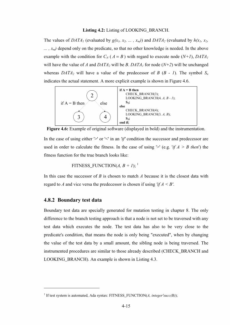
4-15
Listing 4.2: Listing of LOOKING_BRANCH.
The values of DATA1 (evaluated by g(x1, x2, ... , xm)) and DATA2 (evaluated by h(x1, x2,
... , xm) depend only on the predicate, so that no other knowledge is needed. In the above
example with the condition for CN ( A B= ) with regard to execute node (N+1), DATA1
will have the value of A and DATA2 will be B. DATA1 for node (N+2) will be unchanged
whereas DATA2 will have a value of the predecessor of B (B - 1). The symbol Sn
indicates the actual statement. A more explicit example is shown in Figure 4.6.
Figure 4.6: Example of original software (displayed in bold) and the instrumentation.
In the case of using either '>' or '<' in an 'if' condition the successor and predecessor are
used in order to calculate the fitness. In the case of using '>' (e.g. 'if A > B then') the
fitness function for the true branch looks like:
FITNESS_FUNCTION(A, B + 1); 1
In this case the successor of B is chosen to match A because it is the closest data with
regard to A and vice versa the predecessor is chosen if using 'if A < B'.
4.8.2 Boundary test data
Boundary test data are specially generated for mutation testing in chapter 8. The only
difference to the branch testing approach is that a node is not set to be traversed with any
test data which executes the node. The test data has also to be very close to the
predicate's condition, that means the node is only being "executed", when by changing
the value of the test data by a small amount, the sibling node is being traversed. The
instrumented procedures are similar to those already described (CHECK_BRANCH and
LOOKING_BRANCH). An example is shown in Listing 4.3.
1 If test system is automated, Ada syntax: FITNESS_FUNCTION(A, integer'succ(B));
2
3 4
elseif A = B then
if A = B thenCHECK_BRANCH(3);LOOKING_BRANCH(4, A, B - 1);S2;
elseCHECK_BRANCH(4);LOOKING_BRANCH(3, A, B);S3;
end if;
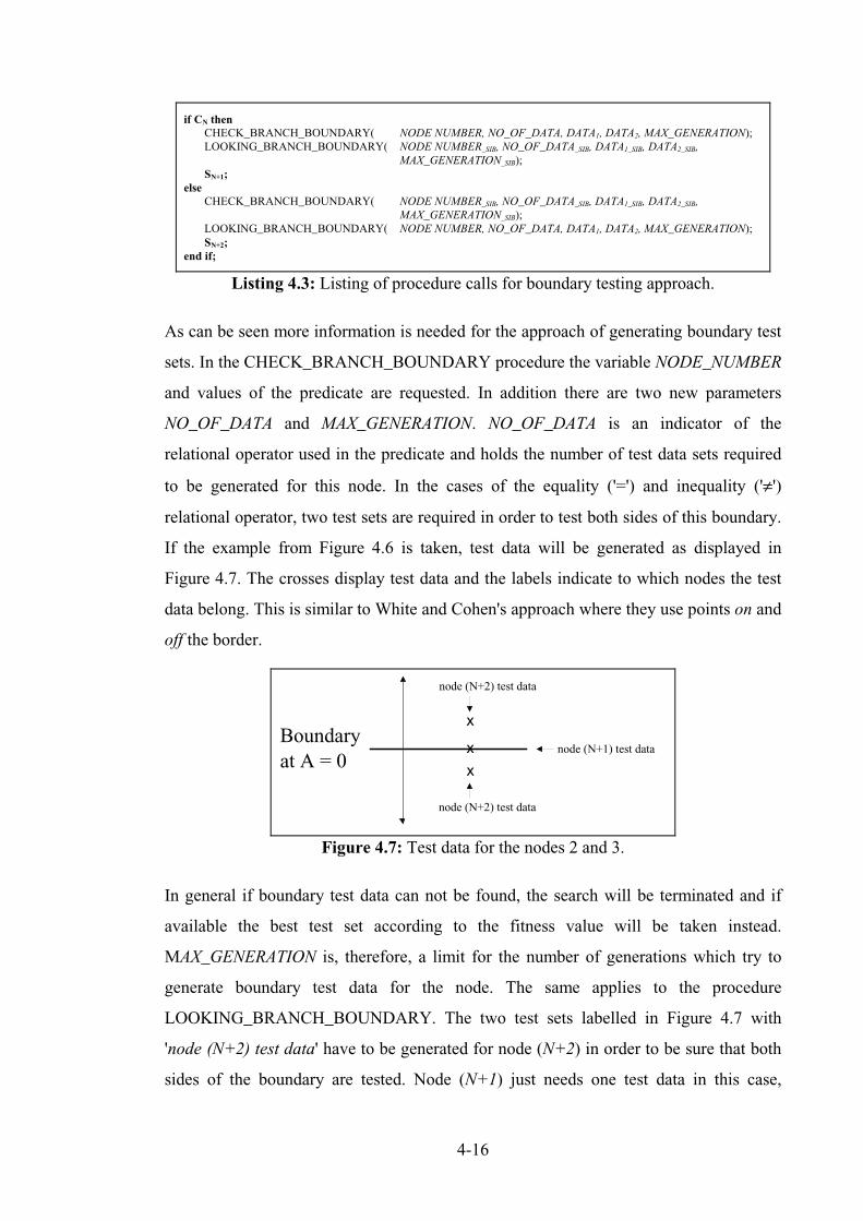
4-16
Listing 4.3: Listing of procedure calls for boundary testing approach.
As can be seen more information is needed for the approach of generating boundary test
sets. In the CHECK_BRANCH_BOUNDARY procedure the variable NODE_NUMBER
and values of the predicate are requested. In addition there are two new parameters
NO_OF_DATA and MAX_GENERATION. NO_OF_DATA is an indicator of the
relational operator used in the predicate and holds the number of test data sets required
to be generated for this node. In the cases of the equality ('=') and inequality ('≠')
relational operator, two test sets are required in order to test both sides of this boundary.
If the example from Figure 4.6 is taken, test data will be generated as displayed in
Figure 4.7. The crosses display test data and the labels indicate to which nodes the test
data belong. This is similar to White and Cohen's approach where they use points on and
off the border.
Figure 4.7: Test data for the nodes 2 and 3.
In general if boundary test data can not be found, the search will be terminated and if
available the best test set according to the fitness value will be taken instead.
MAX_GENERATION is, therefore, a limit for the number of generations which try to
generate boundary test data for the node. The same applies to the procedure
LOOKING_BRANCH_BOUNDARY. The two test sets labelled in Figure 4.7 with
'node (N+2) test data' have to be generated for node (N+2) in order to be sure that both
sides of the boundary are tested. Node (N+1) just needs one test data in this case,
if CN thenCHECK_BRANCH_BOUNDARY( NODE NUMBER, NO_OF_DATA, DATA1, DATA2, MAX_GENERATION);LOOKING_BRANCH_BOUNDARY( NODE NUMBER_SIB, NO_OF_DATA_SIB, DATA1_SIB, DATA2_SIB,
MAX_GENERATION_SIB);SN+1;
elseCHECK_BRANCH_BOUNDARY( NODE NUMBER_SIB, NO_OF_DATA_SIB, DATA1_SIB, DATA2_SIB,
MAX_GENERATION_SIB);LOOKING_BRANCH_BOUNDARY( NODE NUMBER, NO_OF_DATA, DATA1, DATA2, MAX_GENERATION);SN+2;
end if;
at A = 0Boundary
x
x
x node (N+1) test data
node (N+2) test data
node (N+2) test data
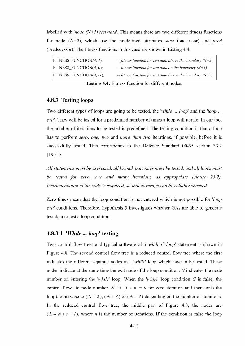
4-17
labelled with 'node (N+1) test data'. This means there are two different fitness functions
for node (N+2), which use the predefined attributes succ (successor) and pred
(predecessor). The fitness functions in this case are shown in Listing 4.4.
Listing 4.4: Fitness function for different nodes.
4.8.3 Testing loops
Two different types of loops are going to be tested, the 'while ... loop' and the 'loop ...
exit'. They will be tested for a predefined number of times a loop will iterate. In our tool
the number of iterations to be tested is predefined. The testing condition is that a loop
has to perform zero, one, two and more than two iterations, if possible, before it is
successfully tested. This corresponds to the Defence Standard 00-55 section 33.2
[1991]:
All statements must be exercised, all branch outcomes must be tested, and all loops must
be tested for zero, one and many iterations as appropriate (clause 23.2).
Instrumentation of the code is required, so that coverage can be reliably checked.
Zero times mean that the loop condition is not entered which is not possible for 'loop
exit' conditions. Therefore, hypothesis 3 investigates whether GAs are able to generate
test data to test a loop condition.
4.8.3.1 'While ... loop' testing
Two control flow trees and typical software of a 'while C loop' statement is shown in
Figure 4.8. The second control flow tree is a reduced control flow tree where the first
indicates the different separate nodes in a 'while' loop which have to be tested. These
nodes indicate at the same time the exit node of the loop condition. N indicates the node
number on entering the 'while' loop. When the 'while' loop condition C is false, the
control flows to node number N + 1 (i.e. n = 0 for zero iteration and then exits the
loop), otherwise to (N + 2 ), (N + 3 ) or (N + 4 ) depending on the number of iterations.
In the reduced control flow tree, the middle part of Figure 4.8, the nodes are
( L N n= + + 1), where n is the number of iterations. If the condition is false the loop
FITNESS_FUNCTION(A, 1); -- fitness function for test data above the boundary (N+2)
FITNESS_FUNCTION(A, 0); -- fitness function for test data on the boundary (N+1)
FITNESS_FUNCTION(A, -1); -- fitness function for test data below the boundary (N+2)

4-18
terminates. S in the software represents some linear statement sequence inside the loop
which executes in node N.
Figure 4.8: Control flow trees of a 'while' loop-statement with the correspondingsoftware.
Iterations are handled in a similar way as 'if' - statements. However, a 'while ... loop'
statement will be tested for zero, one, two and more than two iterations, displayed in
Figure 4.8. The loop is displayed as a dashed line in the reduced control flow tree where
the control flow returns from the end of the loop back to the start of the loop condition.
The additional nodes for the loop iteration testing are numbered as shown in the control
flow tree with L, where L N n= + + 1 and represents the exit node. The '+ 1' expression
is important since the loop is tested for zero iteration which will be a separate node from
the other loop testing nodes. The required number of iterations is analogous to proof by
induction, which means if it is true (true referring to successful testing) for N and N+1
iterations and then true for 1 iteration, it is likely to be true for 2, 3, ..., N iterations.
Therefore, the loop will be handled as four separate nodes. The instrumentation can be
seen in Listing 4.6. Two different procedures have to be instrumented at each node
which are similar to those for an 'if' - statement but which controll the number of
iterations of a conditional loop. The first one is CHECK_BRANCH_LOOP which
checks whether the loop iterated the predefined number of times according to the node
under test. The second one is LOOKING_BRANCH_LOOP which calculates the fitness
value for the node under consideration. The software is displayed in Listing 4.5.
N
N+1
N+2
N+3
N+4
> twice
zero
once
twice
loop
N
L
node L: n = 0 zeronode L: n = 1 oncenode L: n = 2 twicenode L: n = 3 > twice
with L = N + n + 1
Reduced control flow tree
while C loop
S;
end loop;
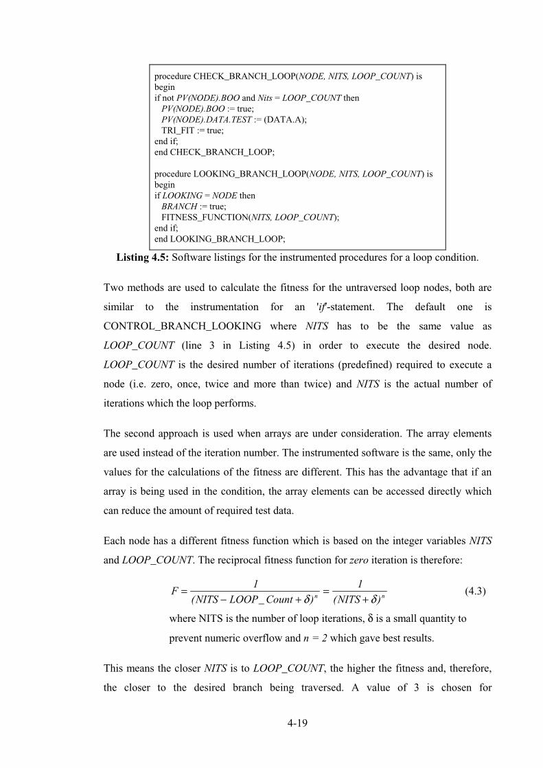
4-19
Listing 4.5: Software listings for the instrumented procedures for a loop condition.
Two methods are used to calculate the fitness for the untraversed loop nodes, both are
similar to the instrumentation for an 'if'-statement. The default one is
CONTROL_BRANCH_LOOKING where NITS has to be the same value as
LOOP_COUNT (line 3 in Listing 4.5) in order to execute the desired node.
LOOP_COUNT is the desired number of iterations (predefined) required to execute a
node (i.e. zero, once, twice and more than twice) and NITS is the actual number of
iterations which the loop performs.
The second approach is used when arrays are under consideration. The array elements
are used instead of the iteration number. The instrumented software is the same, only the
values for the calculations of the fitness are different. This has the advantage that if an
array is being used in the condition, the array elements can be accessed directly which
can reduce the amount of required test data.
Each node has a different fitness function which is based on the integer variables NITS
and LOOP_COUNT. The reciprocal fitness function for zero iteration is therefore:
FNITS LOOP Count NITSn n=
− +=
+1 1
( _ ) ( )δ δ(4.3)
where NITS is the number of loop iterations, δ is a small quantity to
prevent numeric overflow and n = 2 which gave best results.
This means the closer NITS is to LOOP_COUNT, the higher the fitness and, therefore,
the closer to the desired branch being traversed. A value of 3 is chosen for
procedure CHECK_BRANCH_LOOP(NODE, NITS, LOOP_COUNT) isbeginif not PV(NODE).BOO and Nits = LOOP_COUNT then
PV(NODE).BOO := true;PV(NODE).DATA.TEST := (DATA.A);TRI_FIT := true;
end if;end CHECK_BRANCH_LOOP;
procedure LOOKING_BRANCH_LOOP(NODE, NITS, LOOP_COUNT) isbeginif LOOKING = NODE then
BRANCH := true;FITNESS_FUNCTION(NITS, LOOP_COUNT);
end if;end LOOKING_BRANCH_LOOP;

4-20
LOOP_COUNT which corresponds to more than two iterations because it is the
boundary data. A complete instrumentation for loop testing is shown in Listing 4.6.
Listing 4.6: 'while' loop condition with instrumented software.
4.8.3.2 'Loop ... exit' testing
The 'loop ... exit' testing is very similar to the 'while ... loop' testing. The only difference
is that the loop can not be tested for zero iteration since the control has to enter the loop
at least once. This means that the loop can only be tested for one, two and more than two
iterations, represented in Figure 4.9 with the control flow tree and the reduced control
flow tree; the instrumented software is shown in Listing 4.7.
Figure 4.9: Control flow graph of a 'loop ... exit' condition.
The only difference to the previous loop testing approach is that no test is done for zero
iterations.
while C loopNits := Nits + 1;S;
end loop;
CHECK_BRANCH_LOOP(N + 1, NITS, 0);CHECK_BRANCH_LOOP(N + 2, NITS, 1);CHECK_BRANCH_LOOP(N + 3, NITS, 2);CHECK_BRANCH_LOOP(N + 4, NITS, 3);
LOOKING_BRANCH_LOOP(N + 1, NITS, 0);LOOKING_BRANCH_LOOP(N + 2, NITS, 1);LOOKING_BRANCH_LOOP(N + 3, NITS, 2);LOOKING_BRANCH_LOOP(N + 4, NITS, 3);
N
N+1N+2
N+3once
twice
> twice
loop
N
L
node L: n = 1, oncenode L: n = 2, twicenode L: n = 3, > twice
where L = N +n
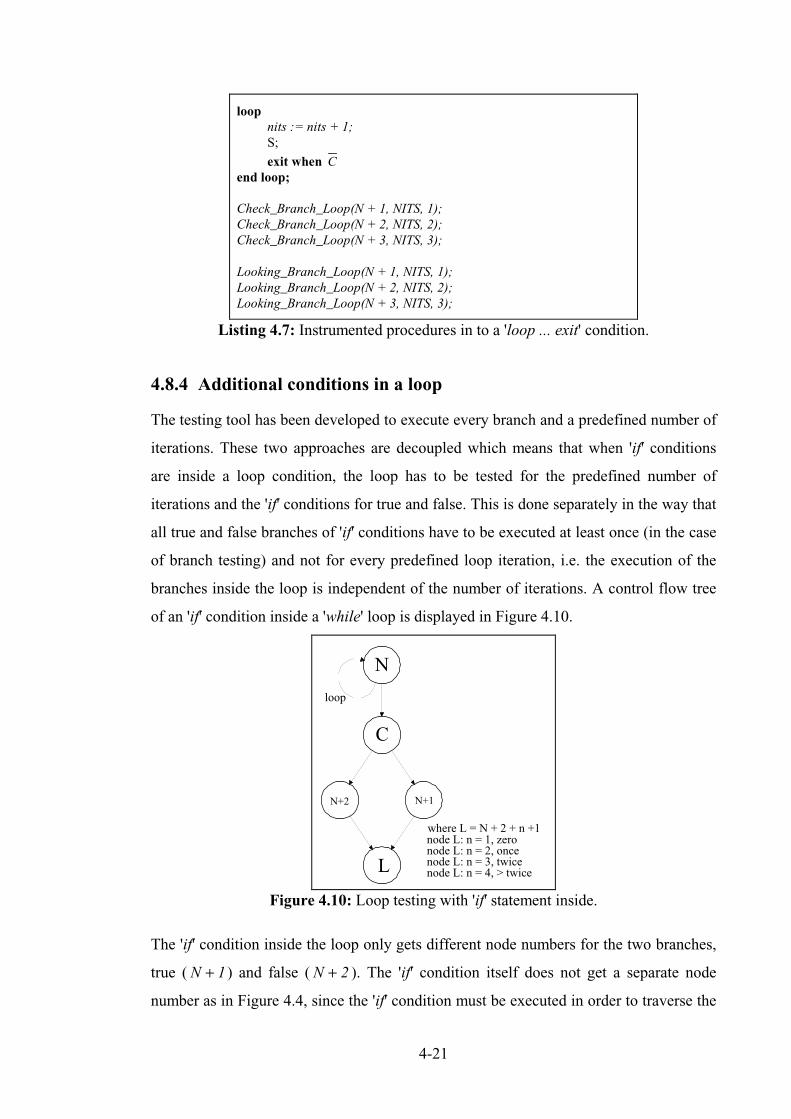
4-21
Listing 4.7: Instrumented procedures in to a 'loop ... exit' condition.
4.8.4 Additional conditions in a loop
The testing tool has been developed to execute every branch and a predefined number of
iterations. These two approaches are decoupled which means that when 'if' conditions
are inside a loop condition, the loop has to be tested for the predefined number of
iterations and the 'if' conditions for true and false. This is done separately in the way that
all true and false branches of 'if' conditions have to be executed at least once (in the case
of branch testing) and not for every predefined loop iteration, i.e. the execution of the
branches inside the loop is independent of the number of iterations. A control flow tree
of an 'if' condition inside a 'while' loop is displayed in Figure 4.10.
loop
N
L
C
N+2 N+1
node L: n = 1, zeronode L: n = 2, oncenode L: n = 3, twicenode L: n = 4, > twice
where L = N + 2 + n +1
Figure 4.10: Loop testing with 'if' statement inside.
The 'if' condition inside the loop only gets different node numbers for the two branches,
true (N + 1 ) and false (N + 2 ). The 'if' condition itself does not get a separate node
number as in Figure 4.4, since the 'if' condition must be executed in order to traverse the
loopnits := nits + 1;S;
exit when Cend loop;
Check_Branch_Loop(N + 1, NITS, 1);Check_Branch_Loop(N + 2, NITS, 2);Check_Branch_Loop(N + 3, NITS, 3);
Looking_Branch_Loop(N + 1, NITS, 1);Looking_Branch_Loop(N + 2, NITS, 2);Looking_Branch_Loop(N + 3, NITS, 3);
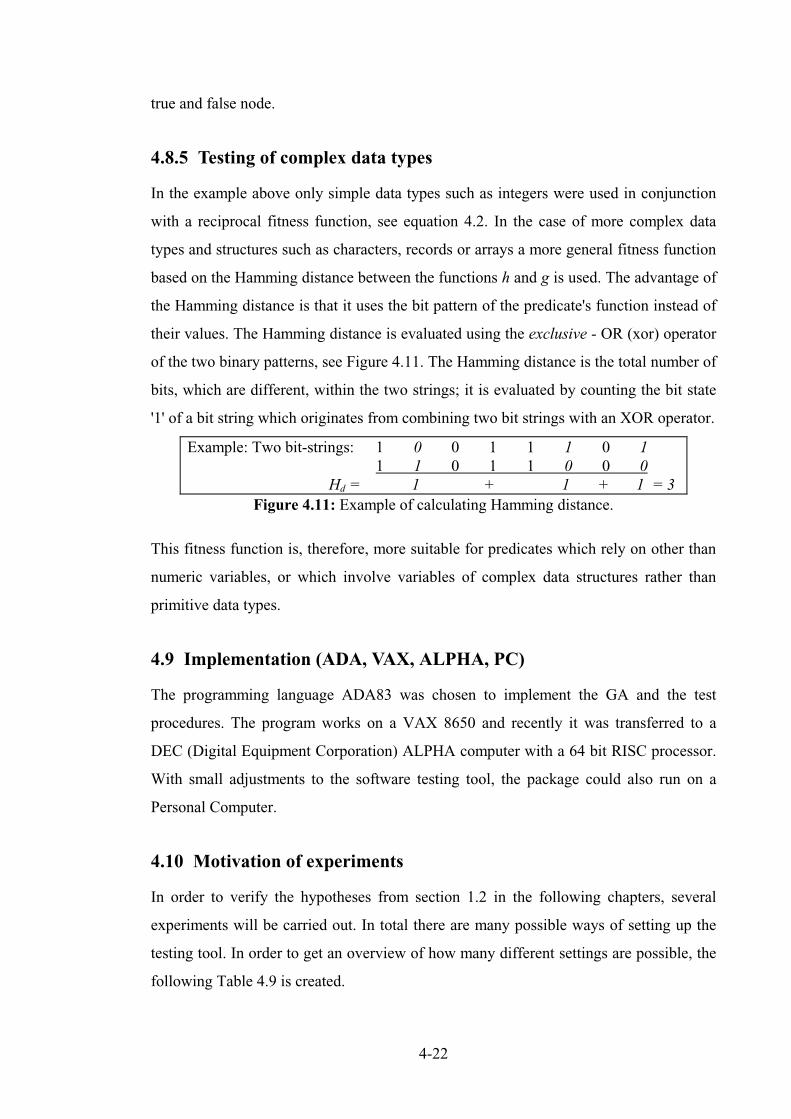
4-22
true and false node.
4.8.5 Testing of complex data types
In the example above only simple data types such as integers were used in conjunction
with a reciprocal fitness function, see equation 4.2. In the case of more complex data
types and structures such as characters, records or arrays a more general fitness function
based on the Hamming distance between the functions h and g is used. The advantage of
the Hamming distance is that it uses the bit pattern of the predicate's function instead of
their values. The Hamming distance is evaluated using the exclusive - OR (xor) operator
of the two binary patterns, see Figure 4.11. The Hamming distance is the total number of
bits, which are different, within the two strings; it is evaluated by counting the bit state
'1' of a bit string which originates from combining two bit strings with an XOR operator.
Figure 4.11: Example of calculating Hamming distance.
This fitness function is, therefore, more suitable for predicates which rely on other than
numeric variables, or which involve variables of complex data structures rather than
primitive data types.
4.9 Implementation (ADA, VAX, ALPHA, PC)
The programming language ADA83 was chosen to implement the GA and the test
procedures. The program works on a VAX 8650 and recently it was transferred to a
DEC (Digital Equipment Corporation) ALPHA computer with a 64 bit RISC processor.
With small adjustments to the software testing tool, the package could also run on a
Personal Computer.
4.10 Motivation of experiments
In order to verify the hypotheses from section 1.2 in the following chapters, several
experiments will be carried out. In total there are many possible ways of setting up the
testing tool. In order to get an overview of how many different settings are possible, the
following Table 4.9 is created.
Example: Two bit-strings: 1 0 0 1 1 1 0 11 1 0 1 1 0 0 0
Hd = 1 + 1 + 1 = 3

4-23
Table 4.9: Possible set-ups.
There is a minimum of about 16.2 ∗ 106 different combinations for the settings using
different methods in GAs, without taking into consideration the size of the population
and the parameter for BITS which determines how many bits should get a higher
probability in W_MUTATE to flip over. This amount of experiments with all different
kind of combinations of parameter and procedures are of course not possible to carry
out. Therefore, selected experiments are carried out, where only one parameter is
changed at the time. The results of these experiments will give knowledge about the
parameter settings and how the GAs react to certain settings. However, additional tests
are required to make sure that the different parameter values do not influence each other,
so that an optimal solution can be found.
These experiments are carried out for all the procedures under test. Only the most
interesting results are listed in the following chapters, where the experiments for the
quadratic procedure are explained in more detail.
Experiments were performed om alternative procedures with the GA settings the same as
those for the quadratic. Those produced by the quadratic procedure and hence are not
mentioned explicitly.
4.11 Interim conclusion
The technique of this approach is white box testing, which means the actual software is
needed for instrumentation and execution (dynamic testing).
The above technique (instrumentation and information transfer to the testing tool) makes
the basic interface possible between the program under test and the test harness. The
testing tool does not need any knowledge of the program's predicates. It needs only to
Possible changes of set-up Number of combinationDifferent crossover 3Crossover probability PC 10Different mutation combination 4Mutation probability Pm 10Selection procedure 3Survive procedure 5Survive probabilities 10Fitness functions 9Gray or binary code 2Threshold of weighted mutation PE 5

4-24
know what kind of input parameters are used, the values of the predicates at run time
and the relational operator used. The adequacy of a test set performance which is
directly related to the fitness value, according to a certain node is obtained via the
predicates.
The number of required iterations can be controlled by LOOP_COUNT and can be
changed. As mentioned earlier the traversing of branches inside a loop is independent of
the number of loop iterations.
In the following chapter experiments are carried out in order to investigate the feasibility
of the applied approach. Several experiments are carried out on two different procedures
under test.
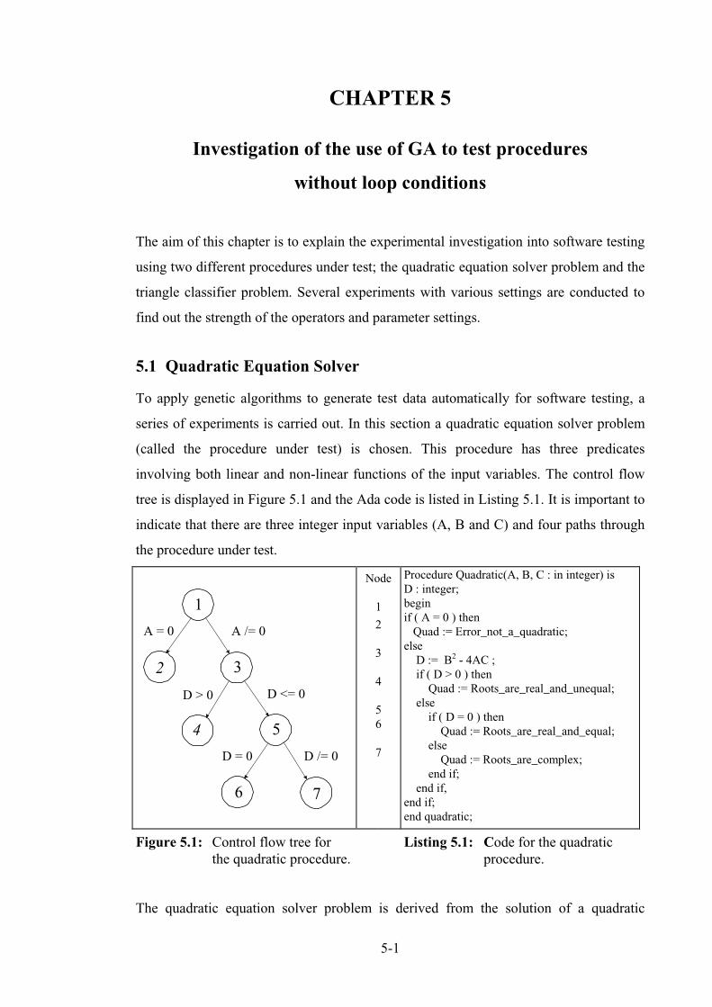
5-1
CHAPTER 5
Investigation of the use of GA to test procedures
without loop conditions
The aim of this chapter is to explain the experimental investigation into software testing
using two different procedures under test; the quadratic equation solver problem and the
triangle classifier problem. Several experiments with various settings are conducted to
find out the strength of the operators and parameter settings.
5.1 Quadratic Equation Solver
To apply genetic algorithms to generate test data automatically for software testing, a
series of experiments is carried out. In this section a quadratic equation solver problem
(called the procedure under test) is chosen. This procedure has three predicates
involving both linear and non-linear functions of the input variables. The control flow
tree is displayed in Figure 5.1 and the Ada code is listed in Listing 5.1. It is important to
indicate that there are three integer input variables (A, B and C) and four paths through
the procedure under test.
1
2 3
4 5
6 7
A = 0 A /= 0
D > 0 D <= 0
D = 0 D /= 0
Node
1
2
3
4
56
7
Procedure Quadratic(A, B, C : in integer) isD : integer;beginif ( A = 0 ) thenQuad := Error_not_a_quadratic;
elseD := B2 - 4AC ;if ( D > 0 ) thenQuad := Roots_are_real_and_unequal;
elseif ( D = 0 ) thenQuad := Roots_are_real_and_equal;
elseQuad := Roots_are_complex;
end if;end if,
end if;end quadratic;
Figure 5.1: Control flow tree forthe quadratic procedure.
Listing 5.1: Code for the quadraticprocedure.
The quadratic equation solver problem is derived from the solution of a quadratic

5-2
equation of the form equation (5.1). The solution is shown in equation (5.2).
Ax Bx C2 0+ + = (5.1)
xB
A
B AC
A1 2
2
2
4
2, = − ± −(5.2)
D B AC= −2 4 (5.3)
The type of result for a quadratic equation depends on the relationship represented in
equation (5.3). The nodes of the control flow tree represent a linear code sequence of
statements between each selection. The leaf nodes 2, 4, 6 and 7 finish with an end if and
will eventually exit the procedure. These nodes represent the different alternatives which
the roots can have (e.g. real, complex, etc.) which will be decided by equation (5.3). If
the conditions are true the next left child node will be executed, if not then the right
node. Nodes 1, 3 and 5 are the branch nodes and they determine the next branch to be
executed depending on its condition and input data. Points to note about the procedure
under test are:
1. One of the input variables, A, is involved directly in an equality condition (A = 0);
2. D is a non-linear function of the input variables, and is involved in two conditions
controlling a total of three paths;
3. D is involved in an equality (D = 0);
If the condition A = 0 is true, node 2 is executed which means that the input variable A
has the value of the constant ( A = 0 ) and indicates that it is not a quadratic equation,
because the first term of equation (5.1) which represents the quadratic characteristic is 0.
Figure 5.2 illustrates global optima (D=0) and local optima (e.g. D = 1 ). The figure
shows a section from the search space in the range from 0 to 40 in only two dimensions
for the input variables A and B with regard to node 6. The default search range is limited
to ±100 for each of the three input variables for the first generation. However, using
GAs and, therefore, crossover and especially mutation operators, test data may be
generated which lie outside of the software input's domain. Those test are invalid for the
software, but it is necessary to use those data to determine the software's response,
Weyuker [1983].
Different symbols indicate different results for D. Circles (o) indicate a global optimum,
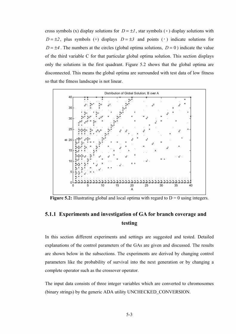
5-3
cross symbols (x) display solutions for D = ±1 , star symbols (∗ ) display solutions with
D = ±2 , plus symbols (+) displays D = ±3 and points ( ⋅ ) indicate solutions for
D = ±4 . The numbers at the circles (global optima solutions, D = 0 ) indicate the value
of the third variable C for that particular global optima solution. This section displays
only the solutions in the first quadrant. Figure 5.2 shows that the global optima are
disconnected. This means the global optima are surrounded with test data of low fitness
so that the fitness landscape is not linear.
0 5 10 15 20 25 30 35 400
5
10
15
20
25
30
35
40Distribution of Global Solution; B over A
A
B
0
1
4
9
16
25
36
49
64
81
100
0
2
8
18
32
50
72
98
0
3
12
27
48
75
0
1
4
9
16
25
36
49
64
81
0
5
20
45
0
6
24
54
0
7
28
0
2
8
18
32
0
1
4
9
16
25
36
0
10
0
11
0
3
12
27
0
13
0
14
0
15
0
1
4
9
16
0
17
0
2
8
18
0
19
0
5
0 0 0 0
6
0
1
4
9
0 0
3
12
0
7
0 0 0 0
2
8
0 0 0 0
1
4
9
0 0 0
Figure 5.2: Illustrating global and local optima with regard to D = 0 using integers.
5.1.1 Experiments and investigation of GA for branch coverage and
testing
In this section different experiments and settings are suggested and tested. Detailed
explanations of the control parameters of the GAs are given and discussed. The results
are shown below in the subsections. The experiments are derived by changing control
parameters like the probability of survival into the next generation or by changing a
complete operator such as the crossover operator.
The input data consists of three integer variables which are converted to chromosomes
(binary strings) by the generic ADA utility UNCHECKED_CONVERSION.

5-4
5.1.1.1 The generic Unchecked_Conversion procedure
The generic UNCHECKED_CONVERSION procedure of ADA, converts any data type
into a two's complement representation. One of the most important features of ADA is
the generic definition. Generic procedures or packages are written in such a general way
that the same algorithm can be applied to variables of any data type. There is no need to
know all the details of these generic types being manipulated. These types together with
procedures which manipulate variables of these types are passed to the generic unit as
parameters when the generic unit is instantiated, Feldman [1993].
An integer conversion will lead to a 32 binary bit array in two's complement format.
This kind of representation is quite different from the representation in binary format
plus sign bit which is shown in Table 5.1 for the numeric value of -1 and +1 with a 8 bit
representation.
Table 5.1: Difference between binary-plus-sign code and two's complementrepresentation.
In the case where a two's complement representation is chosen for mating (crossover),
(e.g. for a negative integer value -1 and positive integer value 1) the offspring are in all
probability totally different from the parents. This is because the patterns of both parent
arrays are very different, compared with the numeric values, see Table 5.1. To avoid
such an effect, a procedure with the name CONTROL_PARENT has been written,
which checks whether a parent has a negative value. In the case of a negative value, it
will be converted into a normal binary with sign coded representation. The MSB
represents the sign bit and is stored by UNCHECKED_CONVERSION on the right side
of the bit array and the LSBs are on the left side.
The patterns of both arrays are now similar as are their numeric values.
5.1.2 Different select procedure
Two chromosomes are selected from the current population for submission to the
crossover and mutation operators. The selection may be made in many ways, either
Bit array Code type decimal value1 1 1 1 1 1 1 1 two's complement -11 0 0 0 0 0 0 0 two's complement 11 0 0 0 0 0 0 1 binary-plus-sign -11 0 0 0 0 0 0 0 binary-plus-sign 1

5-5
purely at random (SELECT_R) or according to the chromosomes' fitness (SELECT_F).
These selection procedures are described in chapter 3.8.2.
5.1.2.1 Results of selection procedures
Experiments are performed with these selection procedures (random and selection
according fitness) in order to find the best way to choose parents for the reproduction
phase. The results show that if the parents with a higher fitness have a better chance of
being selected, they are not as good as an alternative approach where the parents are
completely chosen at random using SELECT_R. In agreement with Lucasius and
Kateman [1993], it is found that the best strategy is to select the parents purely at
random, especially under the present circumstances where there are many global optima
(D = 0) of equal fitness value. Suppose, two chromosomes in one generation might aim
for two different global optima which are in totally different domain areas, so that
although both chromosomes have a high fitness value, the bit patterns are completely
different. If those two chromosomes are selected for recombination, the resulting
offspring could have a very low fitness, because the offspring might be in fact far away
from any global optima, because the offspring might be totally mixed up.
This result is surprising at first sight, but on reflection, random selection maintains a
diversity in the population and this encourages healthy offspring. As has been shown in
other experiments by Lucasius, inbreeding leads to premature convergence at local
optimum solutions which means that the search space is not explored widely enough.
When the parents are selected according to fitness, performance deteriorated. Only 94%
of test runs give complete branch coverage at an average generation of 19.4, giving at
least 2342 tests. This compared to full branch coverage in 13.4 generation (1286 tests)
for random selection. This means that nearly double the number of tests are required in
order to traverse every branch when parents are selected according fitness.
The results, therefore, give a clear statement for hypothesis 2_2 that random selection is
better at least in the cases when several global optima exists.
5.1.3 Different survive procedure
One of the most important operators in the process of GAs is the method of how parents

5-6
and offspring will survive into the next generation, i.e. which individuals of the parent
population are dying and being overwritten by the offspring. In total, five different
survive methods, which are described in chapter 3, are tested thoroughly with different
survive probabilities Ps.
5.1.3.1 Results
The following diagram shows the results of all of the different survive procedures using
the reciprocal fitness function. Figure 5.3 shows the required tests in average over the
probability of survival. The survive procedure which needs fewest tests is the best one,
because it finds a global optimum faster than the others with regard to function
evaluation effort. In order to get a good statistical result, 500 test runs are carried out for
each setup.
Tests required on average for different survivalprocedures
Survival probability
Average
required
tests
0
500
1000
1500
2000
2500
3000
3500
4000
0.1 0.2 0.3 0.4 0.5 0.6 0.7 0.8 0.9 1.0
Survive_1
Survive_3
Survive_4
Survive_5
Figure 5.3: Required tests for different survival procedures and probabilities usingreciprocal fitness function to give branch coverage.
The graph for the results of SURVIVE_2 are omitted from Figure 5.3 because its
survival is independent of PS. The result is about 3254 tests using SURVIVE_2. As can
be seen the best survival strategy is SURVIVE_5 using a reciprocal fitness function
which required fewer tests on average than all other survival procedures. It is not only
the best strategy associated with successful test runs (always 100% success at PS = 0.5),
but it is also the method which generates the most steady and consistent results whatever
the survival probability is. SURVIVE_1 only achieves a similar good result with a very
high survive probability of PS = 1.0. The same experiment is repeated using the
Hamming fitness function. The results are shown in Figure 5.4.
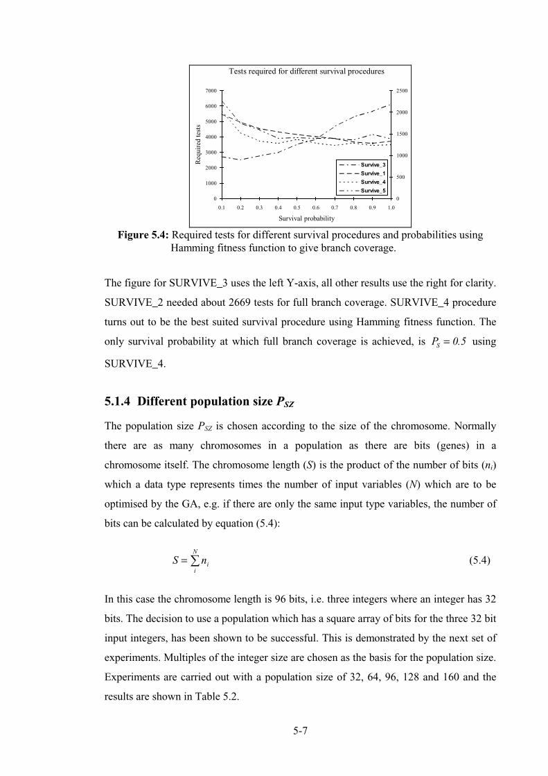
5-7
Tests required for different survival procedures
Survival probability
Requiredtests
0
1000
2000
3000
4000
5000
6000
7000
0.1 0.2 0.3 0.4 0.5 0.6 0.7 0.8 0.9 1.0
0
500
1000
1500
2000
2500
Survive_3
Survive_1
Survive_4
Survive_5
Figure 5.4: Required tests for different survival procedures and probabilities usingHamming fitness function to give branch coverage.
The figure for SURVIVE_3 uses the left Y-axis, all other results use the right for clarity.
SURVIVE_2 needed about 2669 tests for full branch coverage. SURVIVE_4 procedure
turns out to be the best suited survival procedure using Hamming fitness function. The
only survival probability at which full branch coverage is achieved, is PS = 0 5. using
SURVIVE_4.
5.1.4 Different population size PSZ
The population size PSZ is chosen according to the size of the chromosome. Normally
there are as many chromosomes in a population as there are bits (genes) in a
chromosome itself. The chromosome length (S) is the product of the number of bits (ni)
which a data type represents times the number of input variables (N) which are to be
optimised by the GA, e.g. if there are only the same input type variables, the number of
bits can be calculated by equation (5.4):
S nii
N
= � (5.4)
In this case the chromosome length is 96 bits, i.e. three integers where an integer has 32
bits. The decision to use a population which has a square array of bits for the three 32 bit
input integers, has been shown to be successful. This is demonstrated by the next set of
experiments. Multiples of the integer size are chosen as the basis for the population size.
Experiments are carried out with a population size of 32, 64, 96, 128 and 160 and the
results are shown in Table 5.2.
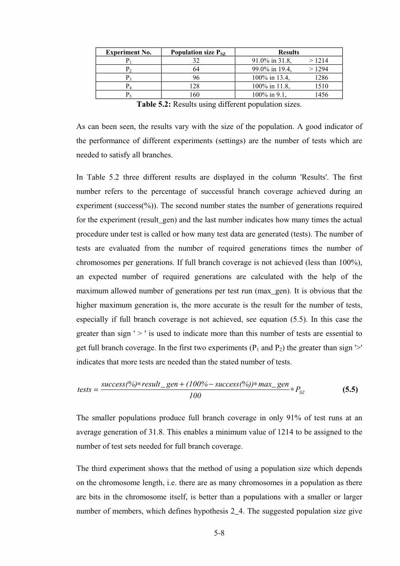
5-8
Table 5.2: Results using different population sizes.
As can been seen, the results vary with the size of the population. A good indicator of
the performance of different experiments (settings) are the number of tests which are
needed to satisfy all branches.
In Table 5.2 three different results are displayed in the column 'Results'. The first
number refers to the percentage of successful branch coverage achieved during an
experiment (success(%)). The second number states the number of generations required
for the experiment (result_gen) and the last number indicates how many times the actual
procedure under test is called or how many test data are generated (tests). The number of
tests are evaluated from the number of required generations times the number of
chromosomes per generations. If full branch coverage is not achieved (less than 100%),
an expected number of required generations are calculated with the help of the
maximum allowed number of generations per test run (max_gen). It is obvious that the
higher maximum generation is, the more accurate is the result for the number of tests,
especially if full branch coverage is not achieved, see equation (5.5). In this case the
greater than sign ' > ' is used to indicate more than this number of tests are essential to
get full branch coverage. In the first two experiments (P1 and P2) the greater than sign '>'
indicates that more tests are needed than the stated number of tests.
testssuccess result gen success gen
PSZ=∗ + − ∗
∗(%) _ ( (%)) max_100%
100(5.5)
The smaller populations produce full branch coverage in only 91% of test runs at an
average generation of 31.8. This enables a minimum value of 1214 to be assigned to the
number of test sets needed for full branch coverage.
The third experiment shows that the method of using a population size which depends
on the chromosome length, i.e. there are as many chromosomes in a population as there
are bits in the chromosome itself, is better than a populations with a smaller or larger
number of members, which defines hypothesis 2_4. The suggested population size give
Experiment No. Population size PSZ ResultsP1 32 91.0% in 31.8, > 1214P2 64 99.0% in 19.4, > 1294P3 96 100% in 13.4, 1286P4 128 100% in 11.8, 1510P5 160 100% in 9.1, 1456

5-9
improved results in the sense that full coverage is obtained in all test runs at an average
of 13.4 generations, corresponding to an average of 1286 tests.
Although, the average number of generations for full branch coverage decreases (100%
in 11.8 generations) the number of required tests (1510) increase, because of the
increase in number of the population size to 128 members.
Small populations usually find solutions quickly, but tend to converge prematurely to a
local optimum. Although in the context of locating members of suitable subdomains,
there may be many goals of equal value, there may be no global optimum in the
normally accepted sense. There is a tendency for the whole population to take the same
value, and this loss of diversity effectively disables the search for the required goal.
Larger populations allow the search space to be sampled more thoroughly and they are
therefore less likely to be trapped by a sub-optimal solution, but the penalty is increased
processing effort (more function evaluation) and it does not mean under any
circumstances that the solution is found in fewer tests. For all future experiments of the
quadratic equation solver a population size of 96 is chosen.
5.1.5 Different fitness functions
The fitness value is calculated by the program under test. The fitness value of an
individual is used to compare an individual with other individuals in the same
population to differentiate their performance with regard to the problem under test. If the
resulting individual is near to the optimum solution, it will get a high fitness value and if
it is far away from the optimum it will get a low fitness value. The better individuals
(higher fitness) usually replicate for mating purposes with a higher probability than the
worse ones which tend to die.
All fitness functions, whether reciprocal or Hamming distance, are derived directly from
the condition of the predicate (objective function).
5.1.5.1 Reciprocal fitness function
The easiest of all the fitness functions used is the reciprocal function. This function is
the reciprocal of the variable to be optimised, see equation (4.2). In trying to satisfy the
predicate D = 0 the fitness of an individual, which has a value of D = 1 , reaches a

5-10
higher level of fitness than an individual with the value of D = 2 (Fitness(D = 1 ) >
Fitness(D = 2 )) because the first individual is closer to satisfying the predicate.
Experiments have consistently shown that the best value for n using equation (4.2) is 2.
The reciprocal fitness function for node 6 is formulated in equation (5.6).
Fitnessh g D
=− +
=− +
αδ
αδ( ) ( )2 20
(5.6)
where δ is a small quantity to prevent numeric overflow,α is a constant (default value is 1) andh and g defines the predicate (see section 4.2.1).
The default setting achieves full branch coverage in 13.4 generations (1286 tests).
5.1.5.2 Gaussian function
The Gaussian distribution is used in order to calculate the fitness of the chromosomes.
The only difference is the shape of the function after the fitness has been calculated.
f x e x( ) = −250
2
2
πφ (5.7)
where φ is a factor in order to change the width of the function and x is
here e.g. D − 0 .
Various parameter values for φ are chosen in order to obtain the best setting. The
disadvantage of the Gaussian and reciprocal approach is that these fitness functions are
only valid for numeric functions. In order to calculate the fitness for non numeric
optimisation problems (characters, records and arrays) a new approach has to be taken.
5.1.5.3 Hamming distance function
The Hamming distance has been implemented using the exclusive OR operator (XOR).
Different variations of the Hamming distances are under investigation; unweighted,
weighted, reciprocal and non-reciprocal.
The simplest form of the Hamming distance is where the bits which have a state of '1'
are counted. This is to be called unweighted Hamming distance (H4 in Table 5.3) . If the
position of the '1' bits are taken into consideration, it is called weighted Hamming
distance. There are different ways of calculating a weighted Hamming distance using

5-11
these bit state positions of '1's which are reflected in the fitness value. H2 squares the bit
position and adds them up whereas H3 only adds up the bit positions. The bit position of
the LSB is 1. H5 calculates the actual bit values of the '1' bits positions and adds these
together. In all these cases, after the distance is determined, the reciprocal of the distance
has to be taken, because the smaller the distance the higher the fitness and the nearer it is
to the global optimum. Another method is to look for bits with the bit state of '0' after
combining two bit strings with an XOR operator (fitness function H1). The effect now is
that the closer the solution is to the global optimum, the higher the total amount of '0's.
Consequently the higher number of ‘0’ is now directly related to the fitness so that there
is no need to take the reciprocal of that value. For node 6 the fitness function could look
like that displayed in Table 5.3 where S is the size of the bit string.
Table 5.3: Different Hamming fitness functions.
The experiments show that the fitness function H2 gives the best results among the
different Hamming fitness functions; the results are shown in Table 5.4.
Table 5.4: Results from using different Hamming fitness functions.
The result when using fitness function H4 is worse than when using the weighted
method H2 or H3, because it does not take into consideration at which position the
difference occurs. A Hamming distance of one between two binary strings can mean in
H1 = D XOR 0 with adding the 0 bit states: Fitnessif
if
H i
H ii
S
= + ���
==
=�δ
1
0
0
11
1
1
( )
( )
Referring to the ith ‘1’ bit state position and using reciprocal:
H2 = D XOR 0 with adding the bits with i2:1
0
1
0
2
1
2
2Fitness
i if
if
H i
H ii
S
= +���
==
=�δ
( )
( )
H3 = D XOR 0 with adding the bits with i:1
0
1
01
3
3Fitness
i if
if
H i
H ii
S
= + ���
==
=�δ
( )
( )
H4 = D XOR 0 with adding the bits with 1;1 1
0
1
01
4
4Fitness
if
if
H i
H ii
S
= + ���
==
=�δ
( )
( )
H5 = D XOR 0 with adding the bits with 2i :1 2
0
1
01
5
5Fitness
if
if
H i
H i
i
i
S
= +���
==
=�δ
( )
( )
Fitness function Result TestsH1 100% in 18.3 generation 1757H2 100% in 14.3 generation 1373H3 100% in 15.2 generation 1460H4 100% in 15.9 generation 1527H5 96.3% in 15.1 generation >1752
5-12
this case that the numerical difference may be very small (e.g. 20) but it can also mean
that the difference may be quite large (e.g. 231) and that the chromosome is numerically
far away from the global optimum.
Using a weighted Hamming fitness avoids this and is used by H2, H3 and H4. This
method will distinguish between chromosomes which are actually close to or far from
the goal using different weighting methods. The results using H5 fitness are not as good
as the other weighted fitness functions. This may be explained by the method being too
strongly weighted. This result is reflected in the experiment when a fitness function is
chosen which is similar to fitness H2, the only difference is that the ith bit position is not
quadrupled (like in H2), it is tripled. An over weighted method will decrease the
performance of the GAs, because the fitness value will always be low until the
individual gets very close to the global optimum.
A comparison between the reciprocal H4 and non reciprocal H1 method, using the same
weighting method, turns out to favour the reciprocal method. The results for the
experiments using H1 are not as good as for the Hamming reciprocal version. The non
reciprocal version H1 needs at least 400 tests more than H2 and about 230 tests more
than H4 until full branch coverage is achieved. The reciprocal effect on the fitness
functions is that closer values (of h and g, see equation (4.1)) are more favoured so that
the GA is directed to these data sets.
A comparison between the different fitness functions shows that using a Hamming
distance as the basis for a fitness function produces more consistent results. By
increasing the range of the initial randomly generated population from ±100 to the range
±200, on average more function evaluations are needed. The reciprocal fitness function
needs at least 3122 tests (91.2% in 26 generations) to obtain full branch coverage
whereas the Hamming distance only needs 1978 tests (20.6 generations) and full branch
coverage is always achieved.
5.1.6 Gray code
The Hamming distance is effective in comparing patterns rather than values. However,
the numbers 7, 8 and 9 are close numerically, but 7 and 8 are separated by a larger
Hamming distance (using binary code) than 8 and 9, this can make the search difficult
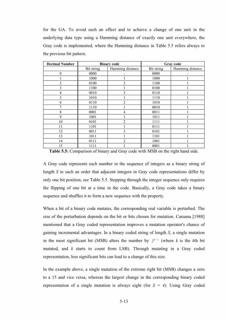
5-13
for the GA. To avoid such an effect and to achieve a change of one unit in the
underlying data type using a Hamming distance of exactly one unit everywhere, the
Gray code is implemented, where the Hamming distance in Table 5.5 refers always to
the previous bit pattern.
Table 5.5: Comparison of binary and Gray code with MSB on the right hand side.
A Gray code represents each number in the sequence of integers as a binary string of
length S in such an order that adjacent integers in Gray code representations differ by
only one bit position, see Table 5.5. Stepping through the integer sequence only requires
the flipping of one bit at a time in the code. Basically, a Gray code takes a binary
sequence and shuffles it to form a new sequence with the property.
When a bit of a binary code mutates, the corresponding real variable is perturbed. The
size of the perturbation depends on the bit or bits chosen for mutation. Caruana [1988]
mentioned that a Gray coded representation improves a mutation operator's chance of
gaining incremental advantages. In a binary coded string of length S, a single mutation
in the most significant bit (MSB) alters the number by 2 1k − (where k is the kth bit
mutated, and k starts to count from LSB). Through mutating in a Gray coded
representation, less significant bits can lead to a change of this size.
In the example above, a single mutation of the extreme right bit (MSB) changes a zero
to a 15 and vice versa, whereas the largest change in the corresponding binary coded
representation of a single mutation is always eight (for S = 4). Using Gray coded
Decimal Number Binary code Gray codeBit string Hamming distance Bit string Hamming distance
0 0000 - 0000 -1 1000 1 1000 12 0100 2 1100 13 1100 1 0100 14 0010 3 0110 15 1010 1 1110 16 0110 2 1010 17 1110 1 0010 18 0001 4 0011 19 1001 1 1011 110 0101 2 1111 111 1101 1 0111 112 0011 3 0101 113 1011 1 1101 114 0111 2 1001 115 1111 1 0001 1
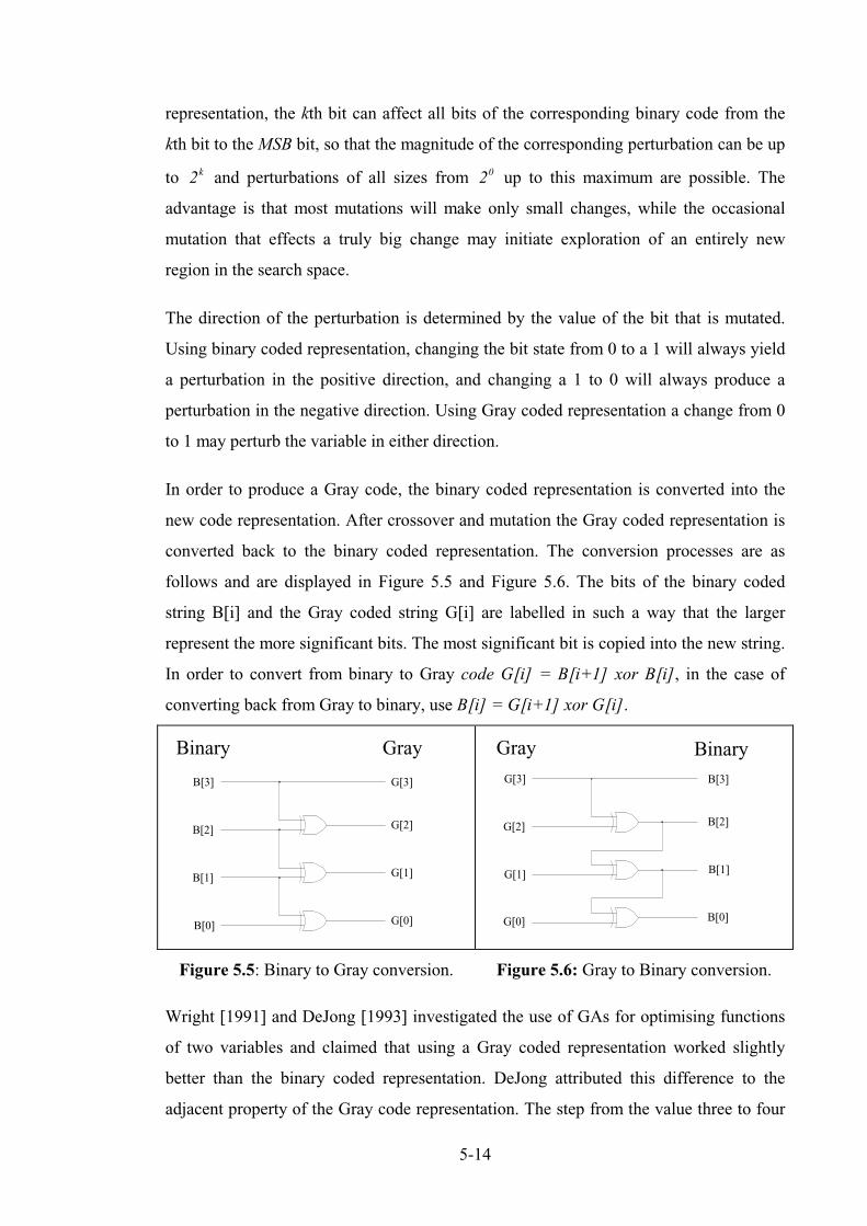
5-14
representation, the kth bit can affect all bits of the corresponding binary code from the
kth bit to the MSB bit, so that the magnitude of the corresponding perturbation can be up
to 2k and perturbations of all sizes from 20 up to this maximum are possible. The
advantage is that most mutations will make only small changes, while the occasional
mutation that effects a truly big change may initiate exploration of an entirely new
region in the search space.
The direction of the perturbation is determined by the value of the bit that is mutated.
Using binary coded representation, changing the bit state from 0 to a 1 will always yield
a perturbation in the positive direction, and changing a 1 to 0 will always produce a
perturbation in the negative direction. Using Gray coded representation a change from 0
to 1 may perturb the variable in either direction.
In order to produce a Gray code, the binary coded representation is converted into the
new code representation. After crossover and mutation the Gray coded representation is
converted back to the binary coded representation. The conversion processes are as
follows and are displayed in Figure 5.5 and Figure 5.6. The bits of the binary coded
string B[i] and the Gray coded string G[i] are labelled in such a way that the larger
represent the more significant bits. The most significant bit is copied into the new string.
In order to convert from binary to Gray code G[i] = B[i+1] xor B[i], in the case of
converting back from Gray to binary, use B[i] = G[i+1] xor G[i].
Wright [1991] and DeJong [1993] investigated the use of GAs for optimising functions
of two variables and claimed that using a Gray coded representation worked slightly
better than the binary coded representation. DeJong attributed this difference to the
adjacent property of the Gray code representation. The step from the value three to four
G[3]
G[2]
G[1]
G[0]
B[3]
B[2]
B[1]
B[0]
Binary GrayG[3]
G[2]
G[1]
G[0]
B[3]
B[2]
B[1]
B[0]
BinaryGray
Figure 5.5: Binary to Gray conversion. Figure 5.6: Gray to Binary conversion.
5-15
requires the flipping of all the bits in the binary representation, as can be seen in the
above example in Table 5.5. In general, adjacent integers in the binary representation
often lie many bit flips apart. This fact makes it less likely that a mutation operator can
effect small changes for a binary coded individual.
5.1.6.1 Results of using Gray code
The results of the experiments using the Gray code are not as good as expected.
Experiments are carried out for both fitness functions. The best results are obtained
using the reciprocal fitness function with only 99.6% success rate in 16.6 generations (>
1626 tests compared to 1286 tests using binary code), but zero solutions ( A ≠ 0 , B = 0 ,
C = 0 ) are only 27% of all test solutions. Since there are fewer zero solutions than using
Gray code means that the pressure towards small values for the input variables A, B and
C is less, and the chance to generate an optimum solution detoriates because the highest
density of global optima is near the origin.
Using the Hamming fitness function H2, only 97.8% successful test runs are achieved in
18.1 generations ( > 1911 tests compared to 1372 tests and 100% success rate using
binary code), however, only 21% zero solutions are generated. For both experiments the
strategy of using the Gray code instead of the binary code increase the number of tests;
in the first case about 350 tests, in the second experiment about 500 tests in order to
achieve full branch coverage.
The results change when W_MUTATE is switched off. Using the reciprocal fitness
function with binary code, the results are much worse. Only 23% of all test runs are
successful in 5.3 generations, compared to using the Gray code, where the success rate is
62.3% in 18.4 generations. By not allowing zero solutions to be a global optima and
using a reciprocal fitness function and binary coding achieved full coverage in 19.7
generations which is about 6.4 generations more than allowing zero solutions, because
there are fewer global optima. However, using Gray code representation achieved
slightly better results in 18.5 generations. This result indicates that Gray code could be
better than binary code (defining hypothesis 2_1) in some cases, especially when zero
values can be avoided. This will be further investigated in the triangle procedure in
section 5.2.
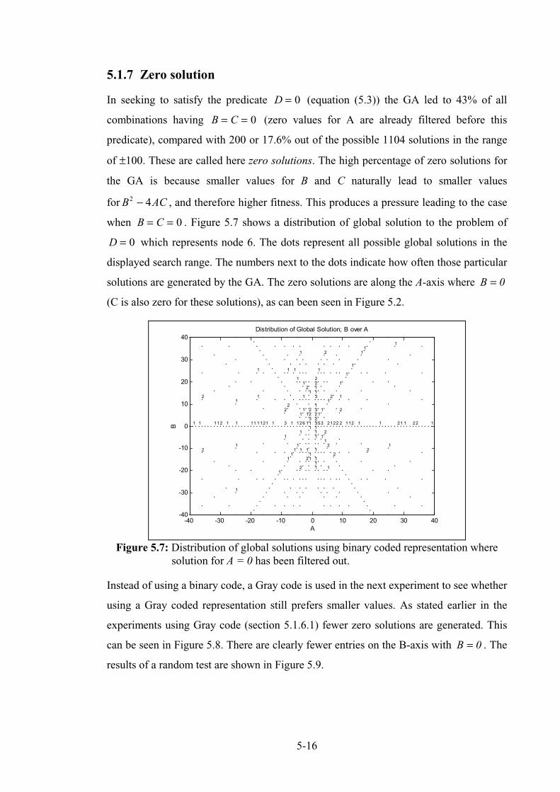
5-16
5.1.7 Zero solution
In seeking to satisfy the predicate D = 0 (equation (5.3)) the GA led to 43% of all
combinations having B C= = 0 (zero values for A are already filtered before this
predicate), compared with 200 or 17.6% out of the possible 1104 solutions in the range
of ±100. These are called here zero solutions. The high percentage of zero solutions for
the GA is because smaller values for B and C naturally lead to smaller values
for B AC2 4− , and therefore higher fitness. This produces a pressure leading to the case
when B C= = 0 . Figure 5.7 shows a distribution of global solution to the problem of
D = 0 which represents node 6. The dots represent all possible global solutions in the
displayed search range. The numbers next to the dots indicate how often those particular
solutions are generated by the GA. The zero solutions are along the A-axis where B = 0
(C is also zero for these solutions), as can been seen in Figure 5.2.
-40 -30 -20 -10 0 10 20 30 40-40
-30
-20
-10
0
10
20
30
40Distribution of Global Solution; B over A
A
B
1 1
2
2
112 1
1
1
1
1 11
1
1
1121 1
1
2
1
3
1
1
2
1
1
1
1
1
1
1
1
2
1
1
1
2
1
1
1
6
2
2
1
1
1
1
1
1
223
11 3
2
1
2
1
3
1
1
3
1
11
1
2
1
2
1
5
1
1
3
1
12
1
2
2
1
2
1
1
2
2
2
2 2
2
1
1
1
1
12
1
1
11
2
1
1
1
21 1 22 1
Figure 5.7: Distribution of global solutions using binary coded representation wheresolution for A = 0 has been filtered out.
Instead of using a binary code, a Gray code is used in the next experiment to see whether
using a Gray coded representation still prefers smaller values. As stated earlier in the
experiments using Gray code (section 5.1.6.1) fewer zero solutions are generated. This
can be seen in Figure 5.8. There are clearly fewer entries on the B-axis with B = 0 . The
results of a random test are shown in Figure 5.9.

5-17
-40 -30 -20 -10 0 10 20 30 40-40
-30
-20
-10
0
10
20
30
40Distribution of Global Solution; B over A
A
B1
1
1
1
1
1
1
1
2 1
1
1
2
1
1
1 1
2
11
1
1
1
1
1
1
1
2
1
1
1
1
1
1
1
1
1
1
1
2
2
1
1
1
2
22
2
42
2
1
33
122
3
1
3
1
211
1
1
2
1
1
2
1
1
1
1
1
2
1
2
1
1
1
1
1
1
2
1
1
1
1
1 31
1
1
1
1 1 1
1
1
1
1
Figure 5.8:Distribution of global solutions using Gray coded representation wheresolution for A = 0 has been filtered out.
-100 -80 -60 -40 -20 0 20 40 60 80 100-100
-80
-60
-40
-20
0
20
40
60
80
100Distribution of Global Solutions; B over A
A
B
2
1
11 1 1
1
1
1
121
1
1
1
1 1
1
1
2
1
11
1
1
1
1
2
1
1
1
1
1
1
1
1
21
111
1
1
2
1
1
1
1
1
1
1
1
1
1
3
1
1
1
1
1
2
1
2
1
1
1
1
1
1
1
1
1
1
1
1
1
1
1
1
1
1
11
1
1
1
1
1
11
1
1
1
1
11
1
1
1
1
1
1
1
1
1
1
11
1
211
1
1
2
1
1
1
1
1
2
1
1
1
11
1
2
1
1
1
1
1
1
1
1
1
1
1
11
1
1
1
1
1
1
1
11
1
1
1
1
1
1
1
1
1
1
1
1
1
1
1
1
1
1
12
1
1
1
1
1
1
1
1
1
1
1
Figure 5.9: Distribution of global solutions using random testing where solution forA = 0 has been filtered out.
As can be seen in the random experiment, Figure 5.9, the generated global solutions are
evenly distributed, whereas the solutions for using GA tends to favour points near the
origin. The results are shown in Figure 5.7 and Figure 5.8 with a limited range. The
entire range is shown for the random experiment.
5.1.8 Comparison of different crossovers
The crossover operator is a process of mixing bit patterns from two guesses
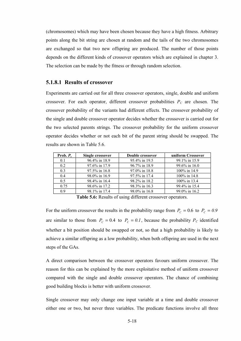
5-18
(chromosomes) which may have been chosen because they have a high fitness. Arbitrary
points along the bit string are chosen at random and the tails of the two chromosomes
are exchanged so that two new offspring are produced. The number of those points
depends on the different kinds of crossover operators which are explained in chapter 3.
The selection can be made by the fitness or through random selection.
5.1.8.1 Results of crossover
Experiments are carried out for all three crossover operators, single, double and uniform
crossover. For each operator, different crossover probabilities PC are chosen. The
crossover probability of the variants had different effects. The crossover probability of
the single and double crossover operator decides whether the crossover is carried out for
the two selected parents strings. The crossover probability for the uniform crossover
operator decides whether or not each bit of the parent string should be swapped. The
results are shown in Table 5.6.
Table 5.6: Results of using different crossover operators.
For the uniform crossover the results in the probability range from PC = 0 6. to PC = 0 9.
are similar to those from PC = 0.4 to PC = 0 1. , because the probability PC identified
whether a bit position should be swapped or not, so that a high probability is likely to
achieve a similar offspring as a low probability, when both offspring are used in the next
steps of the GAs.
A direct comparison between the crossover operators favours uniform crossover. The
reason for this can be explained by the more exploitative method of uniform crossover
compared with the single and double crossover operators. The chance of combining
good building blocks is better with uniform crossover.
Single crossover may only change one input variable at a time and double crossover
either one or two, but never three variables. The predicate functions involve all three
Prob. Pc Single crossover Double crossover uniform Crossover0.1 96.4% in 18.9 95.4% in 19.5 99.1% in 15.90.2 97.6% in 17.9 96.7% in 18.9 99.6% in 16.00.3 97.5% in 16.8 97.0% in 18.8 100% in 14.90.4 98.0% in 16.9 97.5% in 17.4 100% in 14.80.5 98.4% in 16.4 98.2% in 18.2 100% in 13.40.75 98.6% in 17.2 98.3% in 16.3 99.4% in 15.40.9 98.1% in 17.4 98.0% in 16.8 99.0% in 16.2
5-19
variables and a decoupling of any two variables will reduce the effectiveness of the
search for the optimum. In general, uniform crossover explores more of the domain than
1- or 2-point crossover.
Uniform crossover also achieves better results when the input variables are handled
separately and not in one single bit string, so that crossover is applied to each single
input variable (bit string). This can be explained by the length of the input variable and
the range for the first randomly generated population. In order that the offspring are
different from their parents after using single crossover, the crossing point has to be in
the region where bits (genes) have values of '1' which is in most cases the lower
significant bit regions since the input variables have relatively small numeric values
compared to the maximum of + 231 to (-231-1). However, if the crossover point is outside
this region the offspring will not change their pattern and thus can not improve their
genetic material. The chance that the crossover point is in the preferred region is
,therefore, smaller. Uniform crossover does not have this problem because each bit has a
chance of being swapped.
These experiments results conclude that uniform achieves in fewer tests branch coverage
than the other two methods of crossover, defining hypothesis 2_3.
5.1.9 Different mutations
Two different mutation operators are used, MUTATE and W_MUTATE, which are both
described in chapter 3. The best mutation probability turnes out to be Pm = 0.01 in the
experiments which means that on average every 100th gene is swapped, so that there
will be about one mutation per chromosome. This is in agreement with Schaffer's [1987]
and Mühlenbein's [1991 b] suggestion of taking the reciprocal value of the length of a
chromosome as the mutation probability. Therefore, the hypothesis 2_5 is confirmed.
Several tests shown in Table 5.7 are conducted in order to find out which parameter
settings delivere good results.

5-20
Table 5.7: Results of using different mutation probability Pm.
As can be seen if the mutation probability increases the results are worsen. This is
similar to random generated test data, because the GAs cannot use their power to
produce better building blocks because of the changes to the chromosomes are too big.
The same effect regarding the results happens if the mutation probability decreases,
because then there is not enough disruption in the population.
To decide whether the population is stuck at sub-optimal solutions, the procedure
EQUALITY is developed.
5.1.10 The EQUALITY procedure
This procedure determines how many individuals of the current population have the
same value by comparing their fitness values. A population which has many members of
the same individual is unhealthy and risks being stuck at a sub-optimum. If a certain
number of individuals are the same, a flag parameter is set and after the next normal
mutation procedure W_MUTATE will start working. The threshold of starting
W_MUTATE is controlled by the pre-defined parameter PE the equality probability.
Various tests are carried out with different values for PE. The pseudo code of the
EQUALITY procedure can be seen in Figure 5.10 and results in Table 5.8.
Figure 5.10: Pseudo code of EQUALITY procedure.
Probability of Pm Results Tests0.05 82.2% in 36.9 > 46210.025 95.6% in 28.2 > 30110.01 100.0% in 13.4 12870.005 87.4% in 17.3 > 26620.002 63.2% in 14.4 > 4407
Determine how many individuals are the same;if number of same individuals more than a predefined value PE then
use MUTATE and W_MUTATE;else
use only MUTATE;
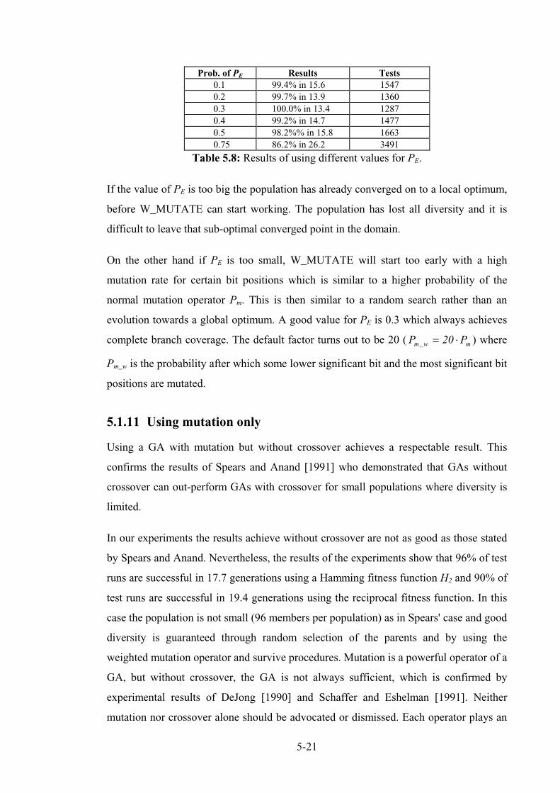
5-21
Table 5.8: Results of using different values for PE.
If the value of PE is too big the population has already converged on to a local optimum,
before W_MUTATE can start working. The population has lost all diversity and it is
difficult to leave that sub-optimal converged point in the domain.
On the other hand if PE is too small, W_MUTATE will start too early with a high
mutation rate for certain bit positions which is similar to a higher probability of the
normal mutation operator Pm. This is then similar to a random search rather than an
evolution towards a global optimum. A good value for PE is 0.3 which always achieves
complete branch coverage. The default factor turns out to be 20 (P Pm w m_ = ⋅20 ) where
Pm_w is the probability after which some lower significant bit and the most significant bit
positions are mutated.
5.1.11 Using mutation only
Using a GA with mutation but without crossover achieves a respectable result. This
confirms the results of Spears and Anand [1991] who demonstrated that GAs without
crossover can out-perform GAs with crossover for small populations where diversity is
limited.
In our experiments the results achieve without crossover are not as good as those stated
by Spears and Anand. Nevertheless, the results of the experiments show that 96% of test
runs are successful in 17.7 generations using a Hamming fitness function H2 and 90% of
test runs are successful in 19.4 generations using the reciprocal fitness function. In this
case the population is not small (96 members per population) as in Spears' case and good
diversity is guaranteed through random selection of the parents and by using the
weighted mutation operator and survive procedures. Mutation is a powerful operator of a
GA, but without crossover, the GA is not always sufficient, which is confirmed by
experimental results of DeJong [1990] and Schaffer and Eshelman [1991]. Neither
mutation nor crossover alone should be advocated or dismissed. Each operator plays an
Prob. of PE Results Tests0.1 99.4% in 15.6 15470.2 99.7% in 13.9 13600.3 100.0% in 13.4 12870.4 99.2% in 14.7 14770.5 98.2%% in 15.8 16630.75 86.2% in 26.2 3491

5-22
important and different role in the search process where crossover is better for achieving
good solutions because crossover shares information between fit individuals whereas
mutation is better for disruption and exploration.
When comparing these results to pure random testing in section 5.1.13 it is found that
the results without crossover are still good. The power of GAs is good at exploiting
solutions even if crossover is not active.
5.1.12 Results of the quadratic equation solver
Many experiments are conducted to investigate which combinations of operator,
probability and methods are best. The best set-up for the GAs for this kind of problem
is:
Uniform crossover with a PC = 0 5. , population size of PSZ = 96, mutation probability of
Pm = 0 01. , SURVIVE_5 with PS = 0 5. , equality probability PE = 0 3. , the reciprocal
fitness function and binary coded sign and magnitude representation have been found to
be the best setting. To check whether this default setting interacts between all other
parameters (probabilities and operators), several additional tests are carried out to
demonstrate whether a good setting has been found.
5.1.13 Random testing
In order to compare the effectiveness of using GA, pure random experiments are carried
out. The input test sets are generated across the range ±100 with a uniform probability.
A total of 7354 random tests are needed to obtain full branch coverage (100% in 76.6
generations) where the limitation of maximum generation (MAX_GEN) per test run is set
to 10000 to ensure that full branch coverage is achieved. If MAX_GEN is restricted to
100 generations only 73.2% of all tests achieve full branch coverage in 40.3 generations,
compared to 1287 tests (100% in 13.4 generations) using GAs.
Poor performance of random testing on such a simple program arise because satisfying
the predicate D = 0 is very difficult compared with the other inequalities. Within the
range ±100, there are over 8 million possible input combinations of A, B and C, but only
1104 (0.014%) will satisfy this predicate. Therefore, the expected number of tests to
execute node 6 can be calculated with equation (5.8):
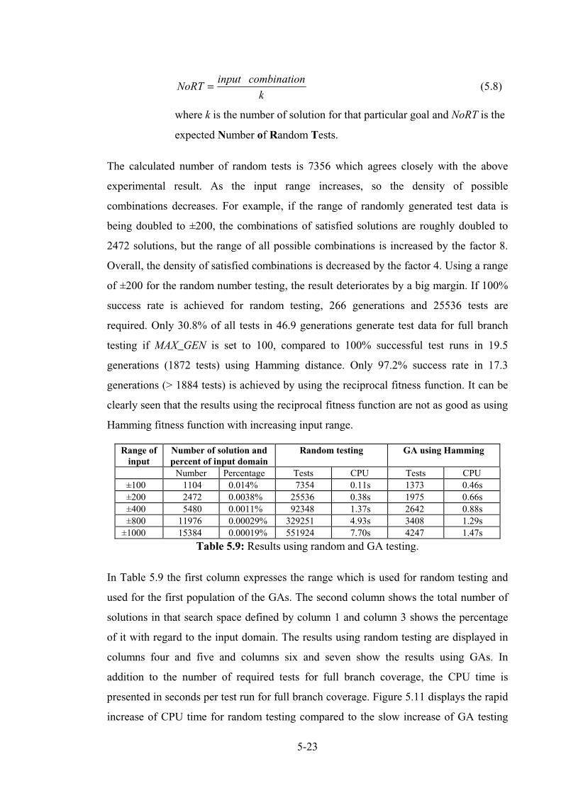
5-23
NoRTinput combination
k= (5.8)
where k is the number of solution for that particular goal and NoRT is the
expected Number of Random Tests.
The calculated number of random tests is 7356 which agrees closely with the above
experimental result. As the input range increases, so the density of possible
combinations decreases. For example, if the range of randomly generated test data is
being doubled to ±200, the combinations of satisfied solutions are roughly doubled to
2472 solutions, but the range of all possible combinations is increased by the factor 8.
Overall, the density of satisfied combinations is decreased by the factor 4. Using a range
of ±200 for the random number testing, the result deteriorates by a big margin. If 100%
success rate is achieved for random testing, 266 generations and 25536 tests are
required. Only 30.8% of all tests in 46.9 generations generate test data for full branch
testing if MAX_GEN is set to 100, compared to 100% successful test runs in 19.5
generations (1872 tests) using Hamming distance. Only 97.2% success rate in 17.3
generations (> 1884 tests) is achieved by using the reciprocal fitness function. It can be
clearly seen that the results using the reciprocal fitness function are not as good as using
Hamming fitness function with increasing input range.
Table 5.9: Results using random and GA testing.
In Table 5.9 the first column expresses the range which is used for random testing and
used for the first population of the GAs. The second column shows the total number of
solutions in that search space defined by column 1 and column 3 shows the percentage
of it with regard to the input domain. The results using random testing are displayed in
columns four and five and columns six and seven show the results using GAs. In
addition to the number of required tests for full branch coverage, the CPU time is
presented in seconds per test run for full branch coverage. Figure 5.11 displays the rapid
increase of CPU time for random testing compared to the slow increase of GA testing
Range ofinput
Number of solution andpercent of input domain
Random testing GA using Hamming
Number Percentage Tests CPU Tests CPU±100 1104 0.014% 7354 0.11s 1373 0.46s±200 2472 0.0038% 25536 0.38s 1975 0.66s±400 5480 0.0011% 92348 1.37s 2642 0.88s±800 11976 0.00029% 329251 4.93s 3408 1.29s±1000 15384 0.00019% 551924 7.70s 4247 1.47s
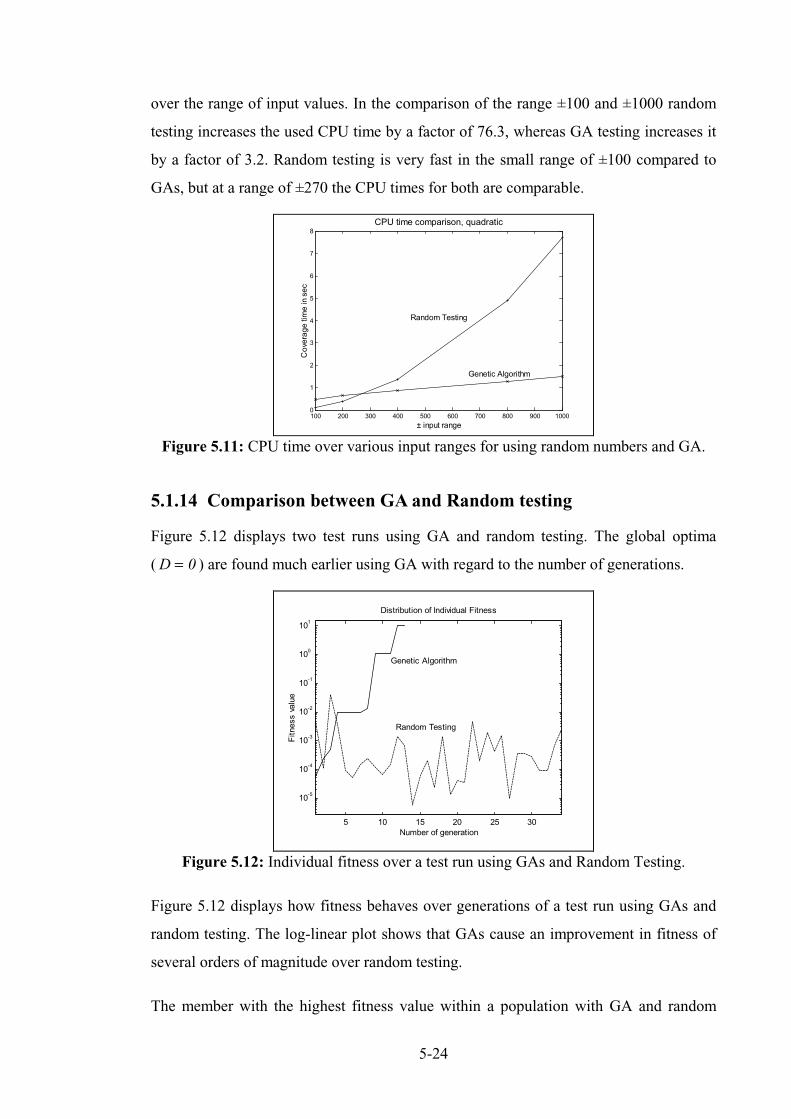
5-24
over the range of input values. In the comparison of the range ±100 and ±1000 random
testing increases the used CPU time by a factor of 76.3, whereas GA testing increases it
by a factor of 3.2. Random testing is very fast in the small range of ±100 compared to
GAs, but at a range of ±270 the CPU times for both are comparable.
100 200 300 400 500 600 700 800 900 10000
1
2
3
4
5
6
7
8
± input range
Coveragetim
einsec
CPU time comparison, quadratic
Genetic Algorithm
Random Testing
Figure 5.11: CPU time over various input ranges for using random numbers and GA.
5.1.14 Comparison between GA and Random testing
Figure 5.12 displays two test runs using GA and random testing. The global optima
(D = 0 ) are found much earlier using GA with regard to the number of generations.
5 10 15 20 25 30
10-5
10-4
10-3
10-2
10-1
100
101
Number of generation
Fitnessvalue
Distribution of Individual Fitness
Genetic Algorithm
Random Testing
Figure 5.12: Individual fitness over a test run using GAs and Random Testing.
Figure 5.12 displays how fitness behaves over generations of a test run using GAs and
random testing. The log-linear plot shows that GAs cause an improvement in fitness of
several orders of magnitude over random testing.
The member with the highest fitness value within a population with GA and random
5-25
testing is printed over the number of generations which displays the off-line
performance (see chapter 3); the fitness values are not accumulated. Once the GA has
started to work, a strong increase in fitness can be observed after only 4 generations
respectively about 400 tests compared with the fitness values of the random testing
method which oscillate around a certain low fitness value. This confirms DeJong's
[1988] statement that typically between 500 and 1000 samples are required before GAs
have sufficient information to explore useful subspaces. The increase in fitness is steady
over the generations until it finds a global optimum in generation 13. The converging
process towards the goal can be seen by the increasing fitness. The fitness values for the
purely random tests are randomly distributed as would be expected.
10 20 30 40 50 60 70 80 90 1000
50
100
150
200
250
300
350
Number of generations
Successfultestruns
Distribution of Test Runs
Genetic Algorithm
Random Testing
Figure 5.13: Histogram of successful test runs.
Figure 5.13 shows distribution / histograms of successful test runs using GAs and
random testing. In both cases 5000 test runs are carried out to get a meaningful
statistical result. The generation numbers in which full branch coverage is achieved are
counted and plotted over the generation range allowable (1 to maximum generation).
The plus (+) symbols indicate the results for the GA and the circles (o) of the random
testing. As can be clearly seen, if using GAs, most of the test runs are successfully
finished in the first 20 generations where its maximum is around generation 7. The
figure strongly decreases after the maximum which is the sign that only a few test runs
require more generations (or tests). However, random testing has not developed such a
strong maximum which is also around generation 7 but it only decreases slowly which is
a sign that many test runs require more generations.
As can be seen from these experiment results generating test data with GAs is more
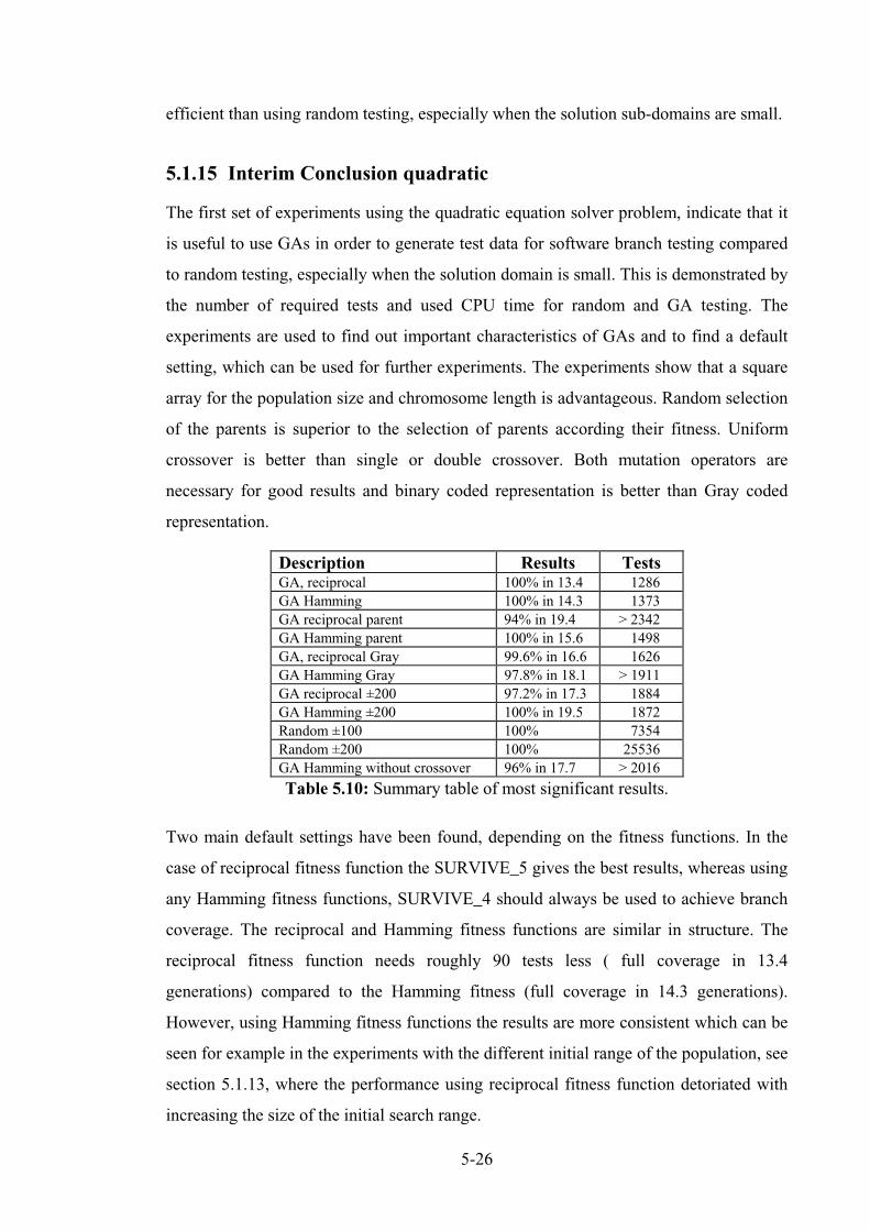
5-26
efficient than using random testing, especially when the solution sub-domains are small.
5.1.15 Interim Conclusion quadratic
The first set of experiments using the quadratic equation solver problem, indicate that it
is useful to use GAs in order to generate test data for software branch testing compared
to random testing, especially when the solution domain is small. This is demonstrated by
the number of required tests and used CPU time for random and GA testing. The
experiments are used to find out important characteristics of GAs and to find a default
setting, which can be used for further experiments. The experiments show that a square
array for the population size and chromosome length is advantageous. Random selection
of the parents is superior to the selection of parents according their fitness. Uniform
crossover is better than single or double crossover. Both mutation operators are
necessary for good results and binary coded representation is better than Gray coded
representation.
Table 5.10: Summary table of most significant results.
Two main default settings have been found, depending on the fitness functions. In the
case of reciprocal fitness function the SURVIVE_5 gives the best results, whereas using
any Hamming fitness functions, SURVIVE_4 should always be used to achieve branch
coverage. The reciprocal and Hamming fitness functions are similar in structure. The
reciprocal fitness function needs roughly 90 tests less ( full coverage in 13.4
generations) compared to the Hamming fitness (full coverage in 14.3 generations).
However, using Hamming fitness functions the results are more consistent which can be
seen for example in the experiments with the different initial range of the population, see
section 5.1.13, where the performance using reciprocal fitness function detoriated with
increasing the size of the initial search range.
Description Results TestsGA, reciprocal 100% in 13.4 1286GA Hamming 100% in 14.3 1373GA reciprocal parent 94% in 19.4 > 2342GA Hamming parent 100% in 15.6 1498GA, reciprocal Gray 99.6% in 16.6 1626GA Hamming Gray 97.8% in 18.1 > 1911GA reciprocal ±200 97.2% in 17.3 1884GA Hamming ±200 100% in 19.5 1872Random ±100 100% 7354Random ±200 100% 25536GA Hamming without crossover 96% in 17.7 > 2016

5-27
The results are promising in that the GAs are able to achieve complete branch coverage
with fewer than 82% of the number of tests that pure random tests require. The results
and analysis of random testing can be divided into two parts. Results which give a
reasonable good performance with test data generated from a small range (±100)
because the density of global solutions is quite high; on the other hand a larger range
(±200) give much worse results because the density of global solutions decrease
strongly and more tests and thus CPU time are required. The main hypothesis 2 can be
confirmed here. A standard setting has been found which will be applied to various
programs under test to verify it and to try to tune and to describe it in more detail.
Both testing methods show that it is quite easy to generate test data for the linear
condition nodes 2 and 3 and for the inequality condition nodes 4 and 7 but for both
methods it is more difficult to generate test data for the non-linear and equality condition
branch node 6. Most of the CPU time is spent producing test data for this particular
node.

5-28
5.2 Triangle classification procedure
Another test procedure is chosen for testing which is similar to the quadratic equation
solver. It is called the triangle classifier procedure and consists of several procedures.
5.2.1 Description of the triangle procedure
The triangle program comprises a combination of three procedures. This program was
written by a member of the research group, Steve Holmes.
The triangle program involves both linear and non-linear functions of the input
variables. Like the quadratic equation solver problem, the triangle also uses equality and
inequality relational operators. The complete triangle program has three integer input
variables A, B and C, one output variable TRI_KIND, 27 nodes, 14 paths and the longest
path has 13 nodes through the software. It is a bigger and more complex procedure than
the quadratic equation solver. The output variable returns the type of triangle
corresponding to the three input variables. The triangle procedure decides whether the
three input variables represent the lengths of the sides of a triangle and determines the
type of the triangle, equilateral, isosceles, scalene or right angled scalene. The name of
the main procedure is TRIANGLE and it has two sub procedures;
RIGHT_ANGLE_CHECK which is also a sub procedure of TRIANGLE_2. The input
variables A, B ,C and the output variable TRI_KIND are global variables in all three
procedures.
The TRIANGLE procedure checks whether the three variables represent a triangle (a
scalene triangle). Therefore the variables have to be greater than the numeric value 0
(corresponding to node 3, 5 and 7, which involves only one variable and a constant at a
time). In addition, twice the value of each single variable has to be less than the
perimeter (P A B C= + + ) value (corresponding node 9, 11 and 13 which involves
linear conditions).
If the test data fulfil all these criteria then the procedure TRIANGLE_2 is called which
determines whether the three variables form an isosceles triangle (represented by node
17, 18 and 21, involve only linear conditions) or an equilateral triangle (node 19).
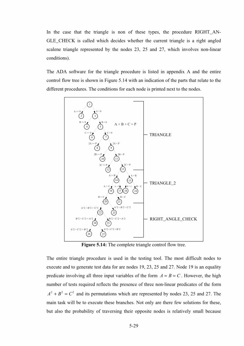
5-29
In the case that the triangle is non of these types, the procedure RIGHT_AN-
GLE_CHECK is called which decides whether the current triangle is a right angled
scalene triangle represented by the nodes 23, 25 and 27, which involves non-linear
conditions).
The ADA software for the triangle procedure is listed in appendix A and the entire
control flow tree is shown in Figure 5.14 with an indication of the parts that relate to the
different procedures. The conditions for each node is printed next to the nodes.
5
9
4
3
6
8
7
10 11
15
12
14
13
19181716
22
20
23
21
26
24
27
25
1
2
A <= 0 A > 0
B <= 0 B > 0
C <= 0 C > 0
2A >= P
2B >= P
2C >= P
2A < P
2B < P
2C < P
A /= B
A /= C
B /= C
A = B
B = CB /= CA = C
A^2 + B^2 /= C^2
B^2 + C^2 /= A^2
A^2 + C^2 /= B^2
A^2 + B^2 = C^2
B^2 + C^2 = A^2
B = C
A^2 + C^2 = B^2
A + B + C = P
TRIANGLE
TRIANGLE_2
RIGHT_ANGLE_CHECK
Figure 5.14: The complete triangle control flow tree.
The entire triangle procedure is used in the testing tool. The most difficult nodes to
execute and to generate test data for are nodes 19, 23, 25 and 27. Node 19 is an equality
predicate involving all three input variables of the form A B C= = . However, the high
number of tests required reflects the presence of three non-linear predicates of the form
A B C2 2 2+ = and its permutations which are represented by nodes 23, 25 and 27. The
main task will be to execute these branches. Not only are there few solutions for these,
but also the probability of traversing their opposite nodes is relatively small because

5-30
many combinations of individuals are already filtered out via the pre-conditions at the
start of the triangle procedure such as all negative values including zero.
5.2.2 Result for the triangle classifier
Several experiments are carried out in order to confirm the performance of the GA. In
particular, different fitness functions and crossover operators are under intense
investigation.
The maximum number of generations after which a test run is abandoned, is increased to
2000, because it is more difficult to generate test data which will satisfy all branches in
the triangle procedure compared to the quadratic equation solver problem.
The results obtained using different fitness functions are similar to the previous set of
experiments for the quadratic problem. The simple reciprocal fitness function achieves
slightly better results than the Hamming fitness functions. The default set-up which has
been derived from the quadratic problem is used for these experiments.
5.2.2.1 Different Fitness functions and survive probabilities
The reciprocal fitness function and default setting leads to 100% successful test runs in
276 generations (27876 tests). With a survival probability of PS = 0 5. , the Hamming
fitness function achieves a success rate of 100%, and the average of the generations
decreased to 270 generations (25945 tests).
5.2.2.2 Different crossover operator
By comparing the different crossover operators, the same kind of result is obtained as in
the quadratic problem. The stated results are obtained with the default setting, which
includes the reciprocal fitness function. Uniform crossover is superior to other crossover
operators (single and double crossover), seen in Table 5.11 where the percentage of full
branch coverage, the number of required generations and tests are displayed.
Table 5.11: Different crossover for the triangle procedure.
Using uniform crossover, complete success (100%) is achieved in 276 generations
Uniform crossover Double crossover Single crossover100% in 276 gen.(27876 tests)
96.3% in 363 gen.(> 40663 tests)
97.5% in 390 gen.(> 41304 tests)

5-31
(27876 tests). Double crossover is only 96.3% successful in 363 generations (> 40663
tests) and single crossover is 97.5% successful in 390 generations (> 41304 tests).
Double and single crossover have almost the same performance, whereas uniform
crossover shows a much better performance, so confirming hypothesis 2_3. When the
crossover operator is completely switched off, only 86.8% of all test runs achieve full
branch coverage in 437 generations. This means that more than 61834 tests must be
completed for full branch coverage to be achieved.
Having used Gray code in the quadratic procedure which achieves slightly better results
than binary code when zero solutions are not allowed, a surprising result is obtained by
using Gray coded representation for the triangle procedure. Using the reciprocal fitness
function, 99.5% of all test runs are successful in only 176 generations which
corresponds to more than 17772 tests and 100% in only 185 generations (17789 tests)
using the Hamming function. The Gray coded representation achieves much better
results (half the number of required tests for branch coverage) than the binary coded
representation for both fitness functions. This confirms hypothesis 2_1 that Gray code
can achieve better results than binary representation.
5.2.3 Comparison with random testing and probabilities
Random testing is also applied to the triangle procedure, to obtain a comparison of the
effectiveness of GAs. In the range ±100 there are only 104 solutions (0.0013%) which
will satisfy the condition A B C2 2 2+ = of node 23, including all pre-conditions. This
means that for node 23 alone an average of 78083 random tests have to be generated in
order to traverse this node. The same probability satisfies nodes 25 and 27 which have
similar conditions, only in a different combination. Most of the CPU time is taken up
traversing these three nodes. However, node 19 which has fewer solutions than any of
these three nodes, is easily traversed by the GA because the predicate of node 19 is
linear whereas the other three are non-linear; it is easier to find one of the global optima
for the linear predicate. Normally for linear conditions, the closer the test data is to the
global optima the higher is the fitness. Thus, the fitness landscape is continuous
increasing so that by favouring always the closer data with a higher fitness value will
eventually generate the optima. On the other hand, if the condition is non-linear, the
fitness landscape also can be non-linear, which means that test data close to a global
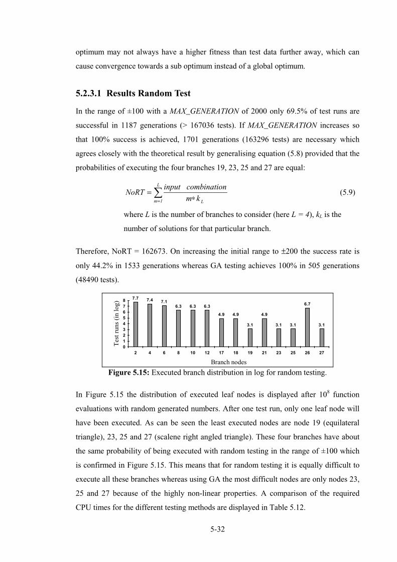
5-32
optimum may not always have a higher fitness than test data further away, which can
cause convergence towards a sub optimum instead of a global optimum.
5.2.3.1 Results Random Test
In the range of ±100 with a MAX_GENERATION of 2000 only 69.5% of test runs are
successful in 1187 generations (> 167036 tests). If MAX_GENERATION increases so
that 100% success is achieved, 1701 generations (163296 tests) are necessary which
agrees closely with the theoretical result by generalising equation (5.8) provided that the
probabilities of executing the four branches 19, 23, 25 and 27 are equal:
NoRTinput combination
m k Lm
L
=∗=
�1
(5.9)
where L is the number of branches to consider (here L = 4), kL is the
number of solutions for that particular branch.
Therefore, NoRT = 162673. On increasing the initial range to ±200 the success rate is
only 44.2% in 1533 generations whereas GA testing achieves 100% in 505 generations
(48490 tests).
Branch nodes
Testruns(inlog)
012345678
2 4 6 8 10 12 17 18 19 21 23 25 26 27
7.7 7.4 7.16.3 6.3 6.3
4.9 4.9
3.1
4.9
3.1 3.1
6.7
3.1
Figure 5.15: Executed branch distribution in log for random testing.
In Figure 5.15 the distribution of executed leaf nodes is displayed after 108 function
evaluations with random generated numbers. After one test run, only one leaf node will
have been executed. As can be seen the least executed nodes are node 19 (equilateral
triangle), 23, 25 and 27 (scalene right angled triangle). These four branches have about
the same probability of being executed with random testing in the range of ±100 which
is confirmed in Figure 5.15. This means that for random testing it is equally difficult to
execute all these branches whereas using GA the most difficult nodes are only nodes 23,
25 and 27 because of the highly non-linear properties. A comparison of the required
CPU times for the different testing methods are displayed in Table 5.12.
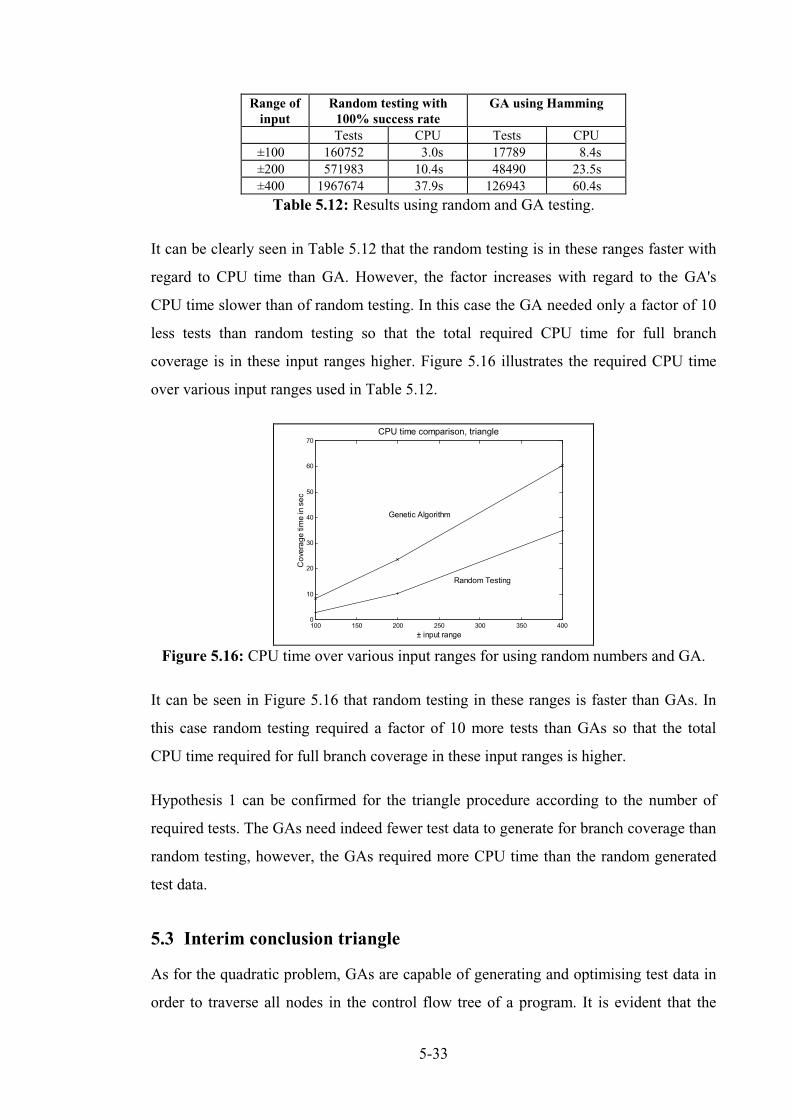
5-33
Table 5.12: Results using random and GA testing.
It can be clearly seen in Table 5.12 that the random testing is in these ranges faster with
regard to CPU time than GA. However, the factor increases with regard to the GA's
CPU time slower than of random testing. In this case the GA needed only a factor of 10
less tests than random testing so that the total required CPU time for full branch
coverage is in these input ranges higher. Figure 5.16 illustrates the required CPU time
over various input ranges used in Table 5.12.
100 150 200 250 300 350 4000
10
20
30
40
50
60
70
± input range
Coveragetim
einsec
CPU time comparison, triangle
Genetic Algorithm
Random Testing
Figure 5.16: CPU time over various input ranges for using random numbers and GA.
It can be seen in Figure 5.16 that random testing in these ranges is faster than GAs. In
this case random testing required a factor of 10 more tests than GAs so that the total
CPU time required for full branch coverage in these input ranges is higher.
Hypothesis 1 can be confirmed for the triangle procedure according to the number of
required tests. The GAs need indeed fewer test data to generate for branch coverage than
random testing, however, the GAs required more CPU time than the random generated
test data.
5.3 Interim conclusion triangle
As for the quadratic problem, GAs are capable of generating and optimising test data in
order to traverse all nodes in the control flow tree of a program. It is evident that the
Range ofinput
Random testing with100% success rate
GA using Hamming
Tests CPU Tests CPU±100 160752 3.0s 17789 8.4s±200 571983 10.4s 48490 23.5s±400 1967674 37.9s 126943 60.4s

5-34
GA's performance is also the superior testing method for the triangle procedure in that it
needs fewer tests. The importance of crossover is demonstrated and is more obvious
than in the quadratic equation solver procedure. Not all of the experiments results are
recorded here. Only the important experiments and results are mentioned in this section
for the triangle procedure. The experiments, that are not explicitly listed in this section,
had a similar outcome as for the quadratic equation procedure, e.g. the survive
procedures and the survive probability.
After a node has been executed the fitness function changes, in order to optimise test
data for the next node. This can be seen in the rapidly decreasing fitness value in Figure
5.17. The labels ‘Node’ express which node is executed at that stage. As earlier stated
the four nodes (19, 23, 25 and 27) are the most difficult ones to execute so that only
these are displayed. Node 23 is traversed in generation 42, node 25 in 63 and node 27 in
generation 65. All other nodes including node 19 are executed in the first 23
generations.
10 20 30 40 50 60 7010-3
10-2
10-1
100
101
102
Generation number
Fitnessvalue
Fitness Distribution using Genetic Algorithm
Node 19
Node 23
Node 25
Node 27
Figure 5.17: Fitness distribution using Genetic Algorithms.
An unexpected result is found when using the Gray code for the chromosomes, instead
of binary format, compared to the results of the quadratic equation solver problem (see
section 5.1.6.1). It indicates that using the Gray code representation of the test data set is
not better than using binary representation if zero solutions are allowed. The better result
obtained using Gray code coincides with those obtained by Schaffer and Caruana et al.
[1991]. They found that using Gray code is often better than using binary coding for
numeric variables. A summary of the most interesting results are shown in Table 5.13.
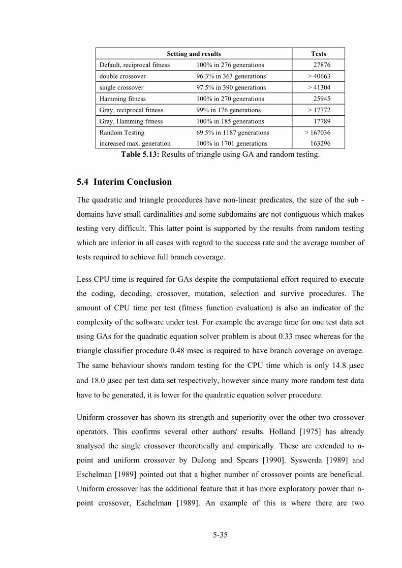
5-35
Table 5.13: Results of triangle using GA and random testing.
5.4 Interim Conclusion
The quadratic and triangle procedures have non-linear predicates, the size of the sub -
domains have small cardinalities and some subdomains are not contiguous which makes
testing very difficult. This latter point is supported by the results from random testing
which are inferior in all cases with regard to the success rate and the average number of
tests required to achieve full branch coverage.
Less CPU time is required for GAs despite the computational effort required to execute
the coding, decoding, crossover, mutation, selection and survive procedures. The
amount of CPU time per test (fitness function evaluation) is also an indicator of the
complexity of the software under test. For example the average time for one test data set
using GAs for the quadratic equation solver problem is about 0.33 msec whereas for the
triangle classifier procedure 0.48 msec is required to have branch coverage on average.
The same behaviour shows random testing for the CPU time which is only 14.8 µsec
and 18.0 µsec per test data set respectively, however since many more random test data
have to be generated, it is lower for the quadratic equation solver procedure.
Uniform crossover has shown its strength and superiority over the other two crossover
operators. This confirms several other authors' results. Holland [1975] has already
analysed the single crossover theoretically and empirically. These are extended to n-
point and uniform crossover by DeJong and Spears [1990]. Syswerda [1989] and
Eschelman [1989] pointed out that a higher number of crossover points are beneficial.
Uniform crossover has the additional feature that it has more exploratory power than n-
point crossover, Eschelman [1989]. An example of this is where there are two
Setting and results Tests
Default, reciprocal fitness 100% in 276 generations 27876
double crossover 96.3% in 363 generations > 40663
single crossover 97.5% in 390 generations > 41304
Hamming fitness 100% in 270 generations 25945
Gray, reciprocal fitness 99% in 176 generations > 17772
Gray, Hamming fitness 100% in 185 generations 17789
Random Testing 69.5% in 1187 generations
increased max. generation 100% in 1701 generations
> 167036
163296

5-36
chromosomes with one of them consisting of a string of 0s and the other one consisting
of 1s. By using uniform crossover the new offspring can be anywhere in the domain,
whereas one or two-point crossovers are restricted to smaller changes in the offspring.
The advantage of a higher exploratory power is ensuring that the entire domain is well
sampled, especially where the population size is small.
The importance of using a crossover operator is clear after the triangle experiments
whereas the results for the quadratic experiments are similar for all crossover operators.
Those results are verified by Schaffer et al. [1989], who mentioned in his work that a
GA even without the assistance of the crossover operator is likely to be a powerful
search algorithm. He also stated that the crossover has an important effect in the GA,
which can be seen in the results of the triangle experiments with and without crossover.
The results indicate that without a crossover operator, the GA is a better search method
than initially expected, but crossover is important.
Having found a default setting for the GAs in this chapter the next chapter will conduct
experiments on more complex data types and structures. Emphasis will be placed on
testing loop conditions.

6-1
CHAPTER 6
The application of GAs to more complex data structure
In the previous chapter a quadratic equation solver and a triangle problem are
investigated. Both programs require three integer input variables. The predicates of the
branches are restricted to selections which contain equality and inequality predicates. In
this chapter more complex data types and iterations are considered. Loops are
considered as four different branches corresponding to zero, one, two and more
iterations. Therefore, in this chapter hypothesis 3 is the main task to validate.
6.1 Search procedures
The application of searching is of great importance in computing, requiring the
development of various techniques in order to test these applications. In this section two
well- known and important algorithms, linear and binary search are tested.
6.1.1 Linear Search_1 procedure
The linear search procedure has two input variables and one output variable. It searches
for the first input variable, X, in an input array A of the size 1..N (second variable) of a
predefined data type (e.g. integer) where the default value for N is 5 in this application.
Using this search method the array element keys are compared with the target key (input
variable X), starting with the first array element. The procedure terminates either when
the target key is located or the end of the array is reached.
N comparisons have to be undertaken to determine the absence of the target key in the
array of N elements. On average N2 comparisons are performed when locating a target
key in an array. The output variable of type boolean indicates whether the key is found
(true) or not (false).
6.1.1.1 Description
The task of the GAs in this program is to adjust the target key (X) to equal one of the
array elements. The default population size is PSZ = 32 chromosomes since only one
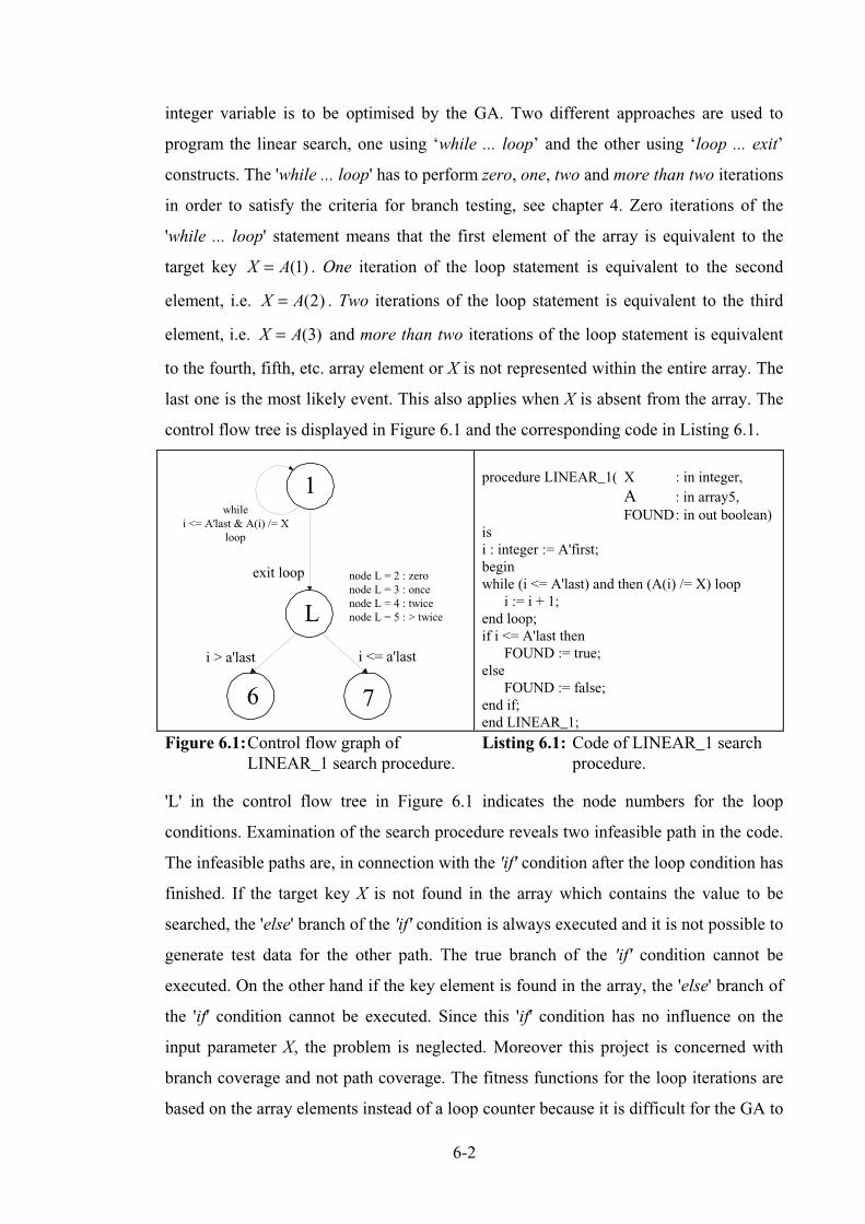
6-2
integer variable is to be optimised by the GA. Two different approaches are used to
program the linear search, one using ‘while ... loop’ and the other using ‘loop ... exit’
constructs. The 'while ... loop' has to perform zero, one, two and more than two iterations
in order to satisfy the criteria for branch testing, see chapter 4. Zero iterations of the
'while ... loop' statement means that the first element of the array is equivalent to the
target key X A= ( )1 . One iteration of the loop statement is equivalent to the second
element, i.e. X A= ( )2 . Two iterations of the loop statement is equivalent to the third
element, i.e. X A= ( )3 and more than two iterations of the loop statement is equivalent
to the fourth, fifth, etc. array element or X is not represented within the entire array. The
last one is the most likely event. This also applies when X is absent from the array. The
control flow tree is displayed in Figure 6.1 and the corresponding code in Listing 6.1.
L
1
6 7
exit loop
i > a'last i <= a'last
whilei <= A'last & A(i) /= X
loop
node L = 2 : zeronode L = 3 : oncenode L = 4 : twicenode L = 5 : > twice
procedure LINEAR_1( X : in integer,A : in array5,FOUND: in out boolean)
isi : integer := A'first;beginwhile (i <= A'last) and then (A(i) /= X) loop
i := i + 1;end loop;if i <= A'last then
FOUND := true;else
FOUND := false;end if;end LINEAR_1;
Figure 6.1:Control flow graph ofLINEAR_1 search procedure.
Listing 6.1: Code of LINEAR_1 searchprocedure.
'L' in the control flow tree in Figure 6.1 indicates the node numbers for the loop
conditions. Examination of the search procedure reveals two infeasible path in the code.
The infeasible paths are, in connection with the 'if' condition after the loop condition has
finished. If the target key X is not found in the array which contains the value to be
searched, the 'else' branch of the 'if' condition is always executed and it is not possible to
generate test data for the other path. The true branch of the 'if' condition cannot be
executed. On the other hand if the key element is found in the array, the 'else' branch of
the 'if' condition cannot be executed. Since this 'if' condition has no influence on the
input parameter X, the problem is neglected. Moreover this project is concerned with
branch coverage and not path coverage. The fitness functions for the loop iterations are
based on the array elements instead of a loop counter because it is difficult for the GA to
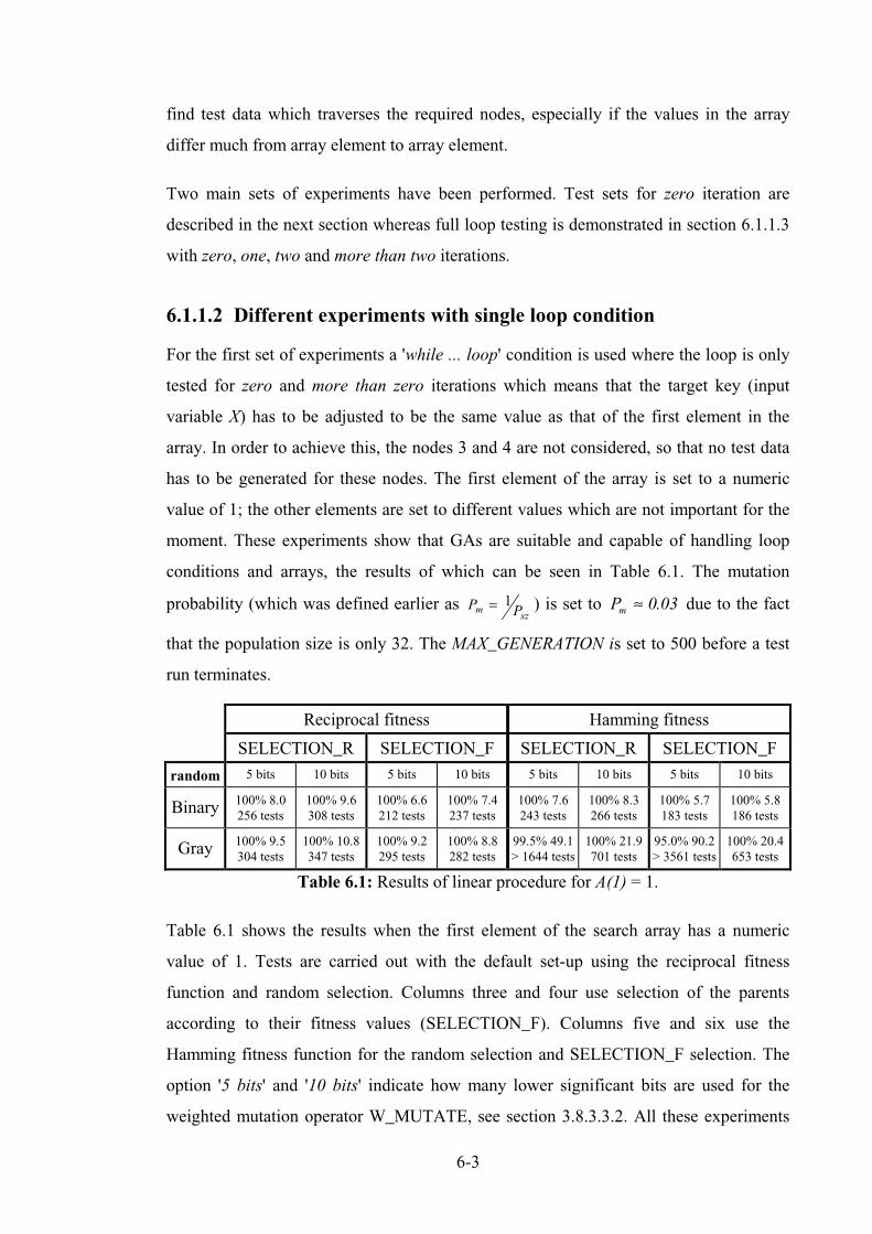
6-3
find test data which traverses the required nodes, especially if the values in the array
differ much from array element to array element.
Two main sets of experiments have been performed. Test sets for zero iteration are
described in the next section whereas full loop testing is demonstrated in section 6.1.1.3
with zero, one, two and more than two iterations.
6.1.1.2 Different experiments with single loop condition
For the first set of experiments a 'while ... loop' condition is used where the loop is only
tested for zero and more than zero iterations which means that the target key (input
variable X) has to be adjusted to be the same value as that of the first element in the
array. In order to achieve this, the nodes 3 and 4 are not considered, so that no test data
has to be generated for these nodes. The first element of the array is set to a numeric
value of 1; the other elements are set to different values which are not important for the
moment. These experiments show that GAs are suitable and capable of handling loop
conditions and arrays, the results of which can be seen in Table 6.1. The mutation
probability (which was defined earlier as P Pmsz
= 1 ) is set to Pm ≈ 0 03. due to the fact
that the population size is only 32. The MAX_GENERATION is set to 500 before a test
run terminates.
Table 6.1: Results of linear procedure for A(1) = 1.
Table 6.1 shows the results when the first element of the search array has a numeric
value of 1. Tests are carried out with the default set-up using the reciprocal fitness
function and random selection. Columns three and four use selection of the parents
according to their fitness values (SELECTION_F). Columns five and six use the
Hamming fitness function for the random selection and SELECTION_F selection. The
option '5 bits' and '10 bits' indicate how many lower significant bits are used for the
weighted mutation operator W_MUTATE, see section 3.8.3.3.2. All these experiments
Reciprocal fitness Hamming fitness
SELECTION_R SELECTION_F SELECTION_R SELECTION_F
random 5 bits 10 bits 5 bits 10 bits 5 bits 10 bits 5 bits 10 bits
Binary 100% 8.0256 tests
100% 9.6308 tests
100% 6.6212 tests
100% 7.4237 tests
100% 7.6243 tests
100% 8.3266 tests
100% 5.7183 tests
100% 5.8186 tests
Gray 100% 9.5304 tests
100% 10.8347 tests
100% 9.2295 tests
100% 8.8282 tests
99.5% 49.1> 1644 tests
100% 21.9701 tests
95.0% 90.2> 3561 tests
100% 20.4653 tests

6-4
are carried out for binary code and Gray code.
As can be seen from Table 6.1, the best results are achieved using the Hamming fitness
function (183 tests) which require about 30 tests fewer than the reciprocal fitness
function. Selection of parents according to fitness (SELECTION_F) produce better
results for both fitness functions than random selection (SELECTION_R) alone. These
are in contradiction to the results achieved with the quadratic and triangle procedures
where SELECTION_F achieves worse results than random selection since there are
many global optima for the nodes. However, in linear search there is just one global
optimum for the node of zero iteration. This is valid for both fitness function methods,
the reciprocal (256 tests) as well as the Hamming (243 tests) fitness functions.
Experiments with Gray code are disappointing with worse results. More than 50 tests are
required to completely achieve successful test runs using reciprocal fitness. The results
deteriorate with the Hamming fitness in particular.
Figure 6.2 shows the population test data set values over the generations and displays
the optimisation process towards the global optimum, which is in this case a value of 1
( X A= =( )1 1) for zero iterations using weighted Hamming fitness function. The plus
symbols in the graph indicate the values of the key target X. Since the population size is
32, there should be 32 stars per generation. However, the scale of the y-axis is quite
large (±20000) which means if the test data are close to each other, it is not possible to
show all test data with separate symbols. This is especially obvious at the end of a test
run where the test data converge towards the global optimum. As can clearly be seen this
set-up avoids all negative values for the test data X (target key) after a few generations,
because a negative number strongly decreases the fitness value due to the weighted
structure of the fitness evaluation.
Assuming that only the MSB, which is the sign bit, has a wrong state (e.g. the current
value is -1 instead of 1) the fitness value will be calculated to 1322 which results in a
very small fitness value so that all negative values are discarded within a certain time.
An example of a test run using the weighted Hamming fitness can be seen in Figure 6.2,
an unweighted Hamming fitness test run is displayed in Figure 6.3 and a reciprocal
fitness test run in Figure 6.4.

6-5
0 2 4 6 8 10 12 14 16 18-2
-1.5
-1
-0.5
0
0.5
1
1.5
2x 10⁴
Generation number
Testdatavalue
Test data converging onto global optimum
Figure 6.2: Converging process towards global optimum using weighted Hammingfitness.
Convergence is slower when negative values are not discarded and unweighted
Hamming fitness is used, see Figure 6.2.
0 5 10 15-2
-1.5
-1
-0.5
0
0.5
1
1.5
2x 10⁴
Generation number
Testdatavalue
Test data converging onto global optimum
Figure 6.3: Converging process towards global optimum using unweighted Hammingfitness.
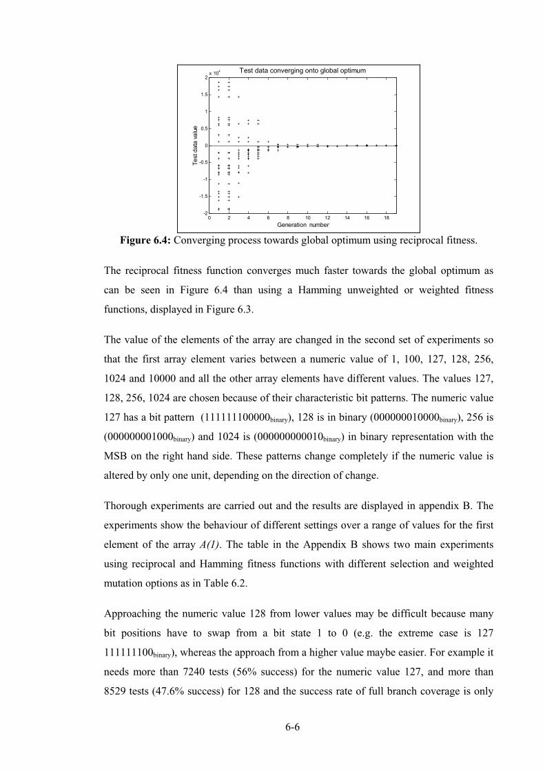
6-6
0 2 4 6 8 10 12 14 16 18-2
-1.5
-1
-0.5
0
0.5
1
1.5
2x 10⁴
Generation number
Testdatavalue
Test data converging onto global optimum
Figure 6.4: Converging process towards global optimum using reciprocal fitness.
The reciprocal fitness function converges much faster towards the global optimum as
can be seen in Figure 6.4 than using a Hamming unweighted or weighted fitness
functions, displayed in Figure 6.3.
The value of the elements of the array are changed in the second set of experiments so
that the first array element varies between a numeric value of 1, 100, 127, 128, 256,
1024 and 10000 and all the other array elements have different values. The values 127,
128, 256, 1024 are chosen because of their characteristic bit patterns. The numeric value
127 has a bit pattern (111111100000binary), 128 is in binary (000000010000binary), 256 is
(000000001000binary) and 1024 is (000000000010binary) in binary representation with the
MSB on the right hand side. These patterns change completely if the numeric value is
altered by only one unit, depending on the direction of change.
Thorough experiments are carried out and the results are displayed in appendix B. The
experiments show the behaviour of different settings over a range of values for the first
element of the array A(1). The table in the Appendix B shows two main experiments
using reciprocal and Hamming fitness functions with different selection and weighted
mutation options as in Table 6.2.
Approaching the numeric value 128 from lower values may be difficult because many
bit positions have to swap from a bit state 1 to 0 (e.g. the extreme case is 127
111111100binary), whereas the approach from a higher value maybe easier. For example it
needs more than 7240 tests (56% success) for the numeric value 127, and more than
8529 tests (47.6% success) for 128 and the success rate of full branch coverage is only

6-7
achieved in about 50% of the test runs using reciprocal fitness function. Whereas it
achieves one of the best results for small values, A(1) = 1, within only 256 tests. As soon
as the values for A(1) increase the results become worse. Using these values, the GA
with reciprocal fitness has great difficulty in generating the global optimum. This means
it is quite difficult to approach these values from one side. If the numeric value is e.g.
1000 the success rate is higher at 88% and only 3967 tests are required and for a value
of 100 the success rate is 99%. This is about half of the required tests which are needed
for a numeric value of A(1) equal to 127 or 128 because the change of the pattern when
approaching those values are not as drastic as for these data.
The option to increase the weighted mutation to '10 bits' is always better except for
small values such as for A(1) = 1. If the values for A(1) are larger, the '10 bits' option
increases the performance enormously, e.g. for A(1) = 128 the success rate is 99.8%
success in >1743 tests, instead of only 47.6% in >8529 tests.
The option SELECTION_F, which selects the parents according to their fitness is only
better for small values of A(1) and achieves the best result within only 212 tests, see
Table 6.1. As soon as the value increases the performance decreases. The degradation in
performance is explained by the tendency of the reciprocal fitness function to favour
smaller values for X. This was realised previously when using the quadratic equation
solver, where solutions with small values for the input variables are favoured over larger
values. The option '10 bits' improves the results using SELECTION_F, because the
chance is higher that several bit positions could change their state in only one
reproduction cycle, but the improvement is higher using it in SELECTION_R.
Gray coding always gives higher success rates and requires fewer tests except for A(1)
= 1 when more tests are needed but full branch coverage is achieved. Full branch
coverage is always achieved with '10 bits'. However, for small values (A(1) = 1) '5 bits'
is better. '5 bits' normally gives worse results in SELECTION_R than in
SELECTION_F, but as soon as the weighted mutation is increased to '10 bits',
SELECTION_F outperformes the option with '5 bits' by far especially for certain bit
patterns, i.e. 100% success is always achieved and it is also better than using it in
SELECTION_R. The performance is influenced by the bit patterns of the numeric
values 127, 128, 256 and 1024. Normally 100% success rate is achieved, but for these

6-8
numeric values only about 96% success is achieved with '5 bits' ('10 bits' always
achieved 100% success).
A fitness function based on the Hamming distance achieves the most consistent
performance in all experiments with respect to success rate and required number of tests.
It is not influenced by certain bit patterns as it is for the reciprocal fitness and it always
achieves a 100% success rate. The number of tests are similar for all different values of
A(1) and only slightly dependent on the setting of the GA with regard to selection and
weighted mutation options. The option of '10 bits' always increases the number of
required tests, no matter which select procedure is chosen. This is in contrast to the
reciprocal fitness which improves the performance in most cases. SELECTION_F
performs better than the random selection for all experiments by about 70 tests.
When using the Gray code representation of the bit pattern, the best results are obtained
with the '10 bits' random selection option and the worst results are obtained when using
the Hamming fitness function.
The best results are achieved with SELECTION_F and '5 bits' using binary coding
which requires about 170 tests for the different A(1) values. In further experiments, the
numeric value for A(1) are generated randomly in the range of ±20000 at the start of
each test run. The results can be seen in Table 6.2.
Table 6.2: Results of generating A(1) randomly for each test run in the range ±20000.
These results confirm the findings of the previous set of experiments. Gray code is better
than binary code for the reciprocal fitness and worse for the Hamming fitness. Hamming
fitness achieves the best results as expected with 183 tests using SELECTION_F and '5
bits'.
The next experiment investigates the case when the array elements A(i) are changed by
Reciprocal fitness Hamming fitness
SELECTION_R SELECTION_F SELECTION_R SELECTION_F
random 5 bits 10 bits 5 bits 10 bits 5 bits 10 bits 5 bits 10 bits
Binary84.6% 63.4>4181 tests
98.4% 29.8>1195 tests
85% 75.3>4450 tests
97.4% 35.3>1518 tests
100% 7.7247 tests
100% 9.1292 tests
100% 5.7183 tests
100% 6.1196 tests
Gray96% 28.0>1501 tests
100% 18.1580 tests
99.8% 19.3>648 tests
99.8% 13.8>475 tests
96.4% 28.1>1442 tests
99.6% 29.3>997 tests
90.4% 29.2>2379 tests
98.6% 22.3>926 tests

6-9
the GA, hence both the key target X and the array elements A(i), requires adjustment. In
this case the array size is restricted to 5 elements, so that the total population is
Psz = ∗ =6 32 192 . The results can be seen in Table 6.3. The maximum generation is
restricted to 100 generations after which a test run terminates because of the amount of
CPU time required.
Table 6.3: Results of linear procedure for zero and more than zero iterations where theelements of the array are also changed by the GAs.
Selection of chromosomes according to their fitness values to become parents for the
next generation is not as good as random selection using reciprocal fitness. This is due
to the fact that there are too many optima which satisfy node 2 (zero iteration node).
Global optima could be anywhere in the search space and not just at the predefined fixed
numeric value of A(1) as in the previous experiments. The resulting disruption might
therefore be too great, as observed when using the triangle and quadratic equation
procedures.
The influence of different sizes of arrays is also investigated. The results of these
experiments show that the outcome is similar to experiments where the population size
is changed in proportion to the integer size for the quadratic equation in section 5. A set
of experiments is carried out where the array consisted of 10 elements. In total
11 32 352∗ = chromosomes per generation are used (key + array elements). 1687 tests
(4.8 generations) are required on average and full coverage is always obtained by using
the Hamming distance fitness function. This test is repeated, but the number of
chromosomes is reduced from 352 to 192. According to expectations the result of 1056
tests (5.5 generations) is similar with regard to the experiment where five array elements
in Table 6.3 are used (1076 tests) within the same setting. Restricting the population
further to 96 chromosomes, full coverage is obtained after only 701 tests (7.3
generations), 64 chromosomes need 557 tests (8.7 generations) and restricting it to 32
chromosomes, branch coverage is achieved only in 378 tests (11.8 generations).
Reciprocal fitness Hamming fitness
SELECTION_R SELECTION_F SELECTION_R SELECTION_F
5 bits 10 bits 5 bits 10 bits 5 bits 10 bits 5 bits 10 bits
77.6%, 7.2>3763 tests
90.8%, 8.2>1711 tests
73.6%, 8.8>4432 tests
76.8%, 12>4007 tests
100%, 18.23495 tests
100%, 17.73399 tests
100% 5.61076 tests
100% 5.91133 tests
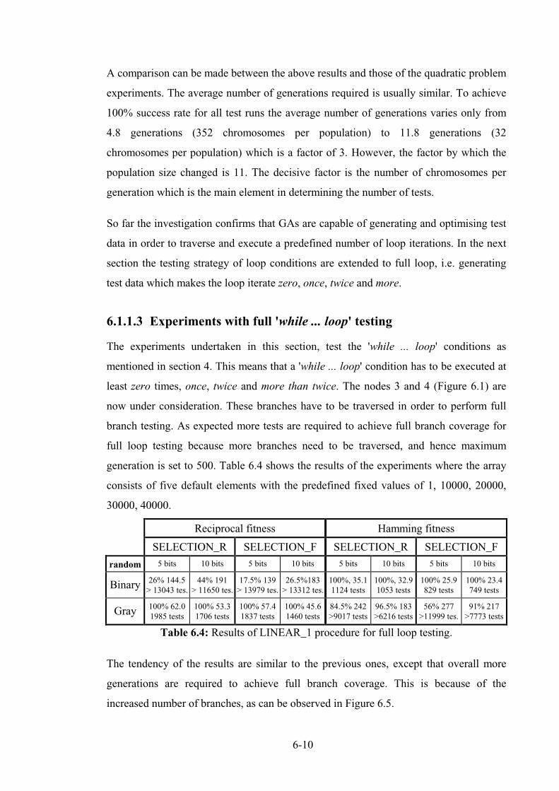
6-10
A comparison can be made between the above results and those of the quadratic problem
experiments. The average number of generations required is usually similar. To achieve
100% success rate for all test runs the average number of generations varies only from
4.8 generations (352 chromosomes per population) to 11.8 generations (32
chromosomes per population) which is a factor of 3. However, the factor by which the
population size changed is 11. The decisive factor is the number of chromosomes per
generation which is the main element in determining the number of tests.
So far the investigation confirms that GAs are capable of generating and optimising test
data in order to traverse and execute a predefined number of loop iterations. In the next
section the testing strategy of loop conditions are extended to full loop, i.e. generating
test data which makes the loop iterate zero, once, twice and more.
6.1.1.3 Experiments with full 'while ... loop' testing
The experiments undertaken in this section, test the 'while ... loop' conditions as
mentioned in section 4. This means that a 'while ... loop' condition has to be executed at
least zero times, once, twice and more than twice. The nodes 3 and 4 (Figure 6.1) are
now under consideration. These branches have to be traversed in order to perform full
branch testing. As expected more tests are required to achieve full branch coverage for
full loop testing because more branches need to be traversed, and hence maximum
generation is set to 500. Table 6.4 shows the results of the experiments where the array
consists of five default elements with the predefined fixed values of 1, 10000, 20000,
30000, 40000.
Table 6.4: Results of LINEAR_1 procedure for full loop testing.
The tendency of the results are similar to the previous ones, except that overall more
generations are required to achieve full branch coverage. This is because of the
increased number of branches, as can be observed in Figure 6.5.
Reciprocal fitness Hamming fitness
SELECTION_R SELECTION_F SELECTION_R SELECTION_F
random 5 bits 10 bits 5 bits 10 bits 5 bits 10 bits 5 bits 10 bits
Binary 26% 144.5> 13043 tes.
44% 191> 11650 tes.
17.5% 139> 13979 tes.
26.5%183> 13312 tes.
100%, 35.11124 tests
100%, 32.91053 tests
100% 25.9829 tests
100% 23.4749 tests
Gray 100% 62.01985 tests
100% 53.31706 tests
100% 57.41837 tests
100% 45.61460 tests
84.5% 242>9017 tests
96.5% 183>6216 tests
56% 277>11999 tes.
91% 217>7773 tests
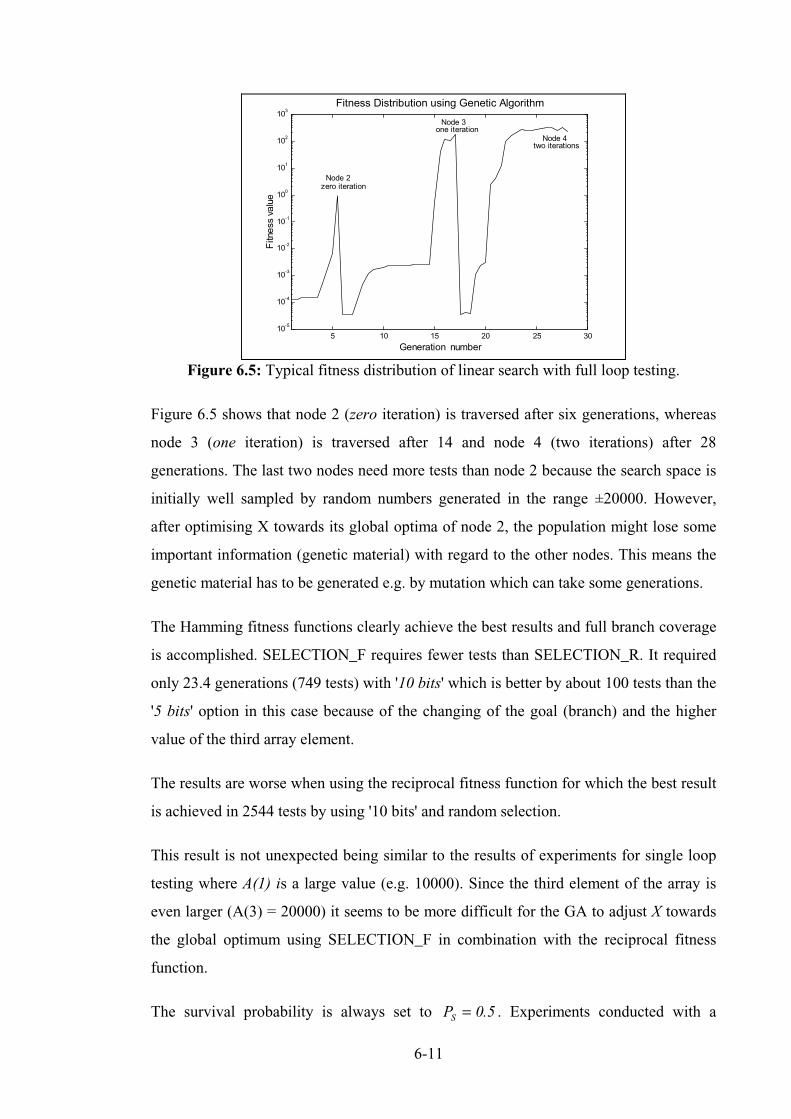
6-11
5 10 15 20 25 3010-5
10-4
10-3
10-2
10-1
100
101
102
103
Generation number
Fitnessvalue
Fitness Distribution using Genetic Algorithm
zero iterationNode 2
one iterationNode 3
two iterationsNode 4
Figure 6.5: Typical fitness distribution of linear search with full loop testing.
Figure 6.5 shows that node 2 (zero iteration) is traversed after six generations, whereas
node 3 (one iteration) is traversed after 14 and node 4 (two iterations) after 28
generations. The last two nodes need more tests than node 2 because the search space is
initially well sampled by random numbers generated in the range ±20000. However,
after optimising X towards its global optima of node 2, the population might lose some
important information (genetic material) with regard to the other nodes. This means the
genetic material has to be generated e.g. by mutation which can take some generations.
The Hamming fitness functions clearly achieve the best results and full branch coverage
is accomplished. SELECTION_F requires fewer tests than SELECTION_R. It required
only 23.4 generations (749 tests) with '10 bits' which is better by about 100 tests than the
'5 bits' option in this case because of the changing of the goal (branch) and the higher
value of the third array element.
The results are worse when using the reciprocal fitness function for which the best result
is achieved in 2544 tests by using '10 bits' and random selection.
This result is not unexpected being similar to the results of experiments for single loop
testing where A(1) is a large value (e.g. 10000). Since the third element of the array is
even larger (A(3) = 20000) it seems to be more difficult for the GA to adjust X towards
the global optimum using SELECTION_F in combination with the reciprocal fitness
function.
The survival probability is always set to PS = 0 5. . Experiments conducted with a
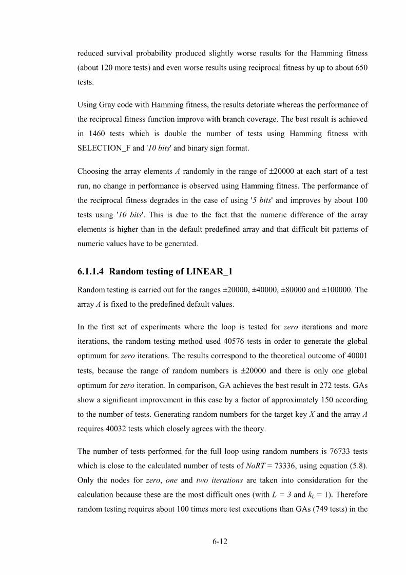
6-12
reduced survival probability produced slightly worse results for the Hamming fitness
(about 120 more tests) and even worse results using reciprocal fitness by up to about 650
tests.
Using Gray code with Hamming fitness, the results detoriate whereas the performance of
the reciprocal fitness function improve with branch coverage. The best result is achieved
in 1460 tests which is double the number of tests using Hamming fitness with
SELECTION_F and '10 bits' and binary sign format.
Choosing the array elements A randomly in the range of ±20000 at each start of a test
run, no change in performance is observed using Hamming fitness. The performance of
the reciprocal fitness degrades in the case of using '5 bits' and improves by about 100
tests using '10 bits'. This is due to the fact that the numeric difference of the array
elements is higher than in the default predefined array and that difficult bit patterns of
numeric values have to be generated.
6.1.1.4 Random testing of LINEAR_1
Random testing is carried out for the ranges ±20000, ±40000, ±80000 and ±100000. The
array A is fixed to the predefined default values.
In the first set of experiments where the loop is tested for zero iterations and more
iterations, the random testing method used 40576 tests in order to generate the global
optimum for zero iterations. The results correspond to the theoretical outcome of 40001
tests, because the range of random numbers is ±20000 and there is only one global
optimum for zero iteration. In comparison, GA achieves the best result in 272 tests. GAs
show a significant improvement in this case by a factor of approximately 150 according
to the number of tests. Generating random numbers for the target key X and the array A
requires 40032 tests which closely agrees with the theory.
The number of tests performed for the full loop using random numbers is 76733 tests
which is close to the calculated number of tests of NoRT = 73336, using equation (5.8).
Only the nodes for zero, one and two iterations are taken into consideration for the
calculation because these are the most difficult ones (with L = 3 and kL = 1). Therefore
random testing requires about 100 times more test executions than GAs (749 tests) in the
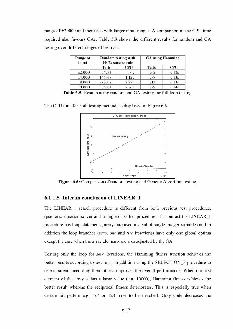
6-13
range of ±20000 and increases with larger input ranges. A comparison of the CPU time
required also favours GAs. Table 5.9 shows the different results for random and GA
testing over different ranges of test data.
Table 6.5: Results using random and GA testing for full loop testing.
The CPU time for both testing methods is displayed in Figure 6.6.
2 3 4 5 6 7 8 9 10
x 104
0
0.5
1
1.5
2
2.5
3
± input range
Coveragetim
einsec
CPU time comparison, linear
Genetic Algorithm
Random Testing
Figure 6.6: Comparison of random testing and Genetic Algorithm testing.
6.1.1.5 Interim conclusion of LINEAR_1
The LINEAR_1 search procedure is different from both previous test procedures,
quadratic equation solver and triangle classifier procedures. In contrast the LINEAR_1
procedure has loop statements, arrays are used instead of single integer variables and in
addition the loop branches (zero, one and two iterations) have only one global optima
except the case when the array elements are also adjusted by the GA.
Testing only the loop for zero iterations, the Hamming fitness function achieves the
better results according to test runs. In addition using the SELECTION_F procedure to
select parents according their fitness improves the overall performance. When the first
element of the array A has a large value (e.g. 10000), Hamming fitness achieves the
better result whereas the reciprocal fitness deteriorates. This is especially true when
certain bit pattern e.g. 127 or 128 have to be matched. Gray code decreases the
Range ofinput
Random testing with100% success rate
GA using Hamming
Tests CPU Tests CPU±20000 76733 0.6s 762 0.12s±40000 146637 1.12s 788 0.13s±80000 298058 2.27s 813 0.13s±100000 375661 2.86s 829 0.14s

6-14
performance of Hamming fitness whereas using SELECTION_F improves the
performance by about 2 to 3 generations so that only about 160 tests are required.
The third part of these experiments is carried out with full testing of the loop condition.
Gray code invariably performs better when it is used with the reciprocal fitness, as
already stated in the earlier experiments. When using Gray code in conjunction with
Hamming fitness, the results deteriorate strongly.
The selection of parents using the fitness value (SELECTION_F) always works very
well for the Hamming fitness but slightly worse using the reciprocal fitness function.
When tested in connection with Gray code and SELECTION_F the reciprocal fitness
function achieves better results than without it. Overall the Hamming fitness function
achieves the most consistent results over a large range of different values for the global
optimum.

6-15
6.1.2 Linear Search 2
The control flow graph of LINEAR_2 procedure is given in Figure 6.7 and the code is
shown in Listing 6.2. The LINEAR_2 procedure is similar to LINEAR_1, the only
difference is that instead of a ‘while ... loop’ a ‘loop ... exit’ condition is used. In
addition two 'if' conditions are used in order to exit the loop. The testing goal is branch
coverage. The first 'if' condition node 2 terminates the loop when the index i is beyond
the maximum index of the array A. When the second 'if' condition is true (node 4), the
loop is exited because the key element X matches one of the array elements A(i).
1
C
C
3 2
loop exitnode L = 6 : oncenode L = 7 : twicenode L = 8 : > twice
L
5 4
9 10
i > a'last i <= a'last
i > a'last
A(i) = X
C
exit
exit
procedure LINEAR_2(X : in out integer,FOUND : in out boolean) is
i := A'first;beginloopif i > A'last thenexit
end if;if A(i) = x thenexit;
end if;i := i + 1;
end loop;if i ≤ A'last thenFound := true;
elseFound := false;
end if;end LINEAR_2;
Figure 6.7:Control flow graph ofLINEAR_2 procedure.
Listing 6.2: Code of LINEAR_2 searchprocedure.
The method of testing a 'loop exit' condition has to be changed because the loop has to
be entered at least once, i.e. it is tested for one, two and more than two iterations where
one iteration means X = A(1). Because of the semantics of the 'loop...exit' construct, zero
iterations cannot be tested. In addition the 'else' branches of the 'if' conditions inside the
loop have both been tested to make sure that the 'if' condition is not always being
executed.
Since the two search procedures are very similar, LINEAR_2 is only tested for full loop
testing. The array elements are fixed to the predefined default values of (1, 10000,
20000, 30000, 40000). The results are shown in Table 6.6.
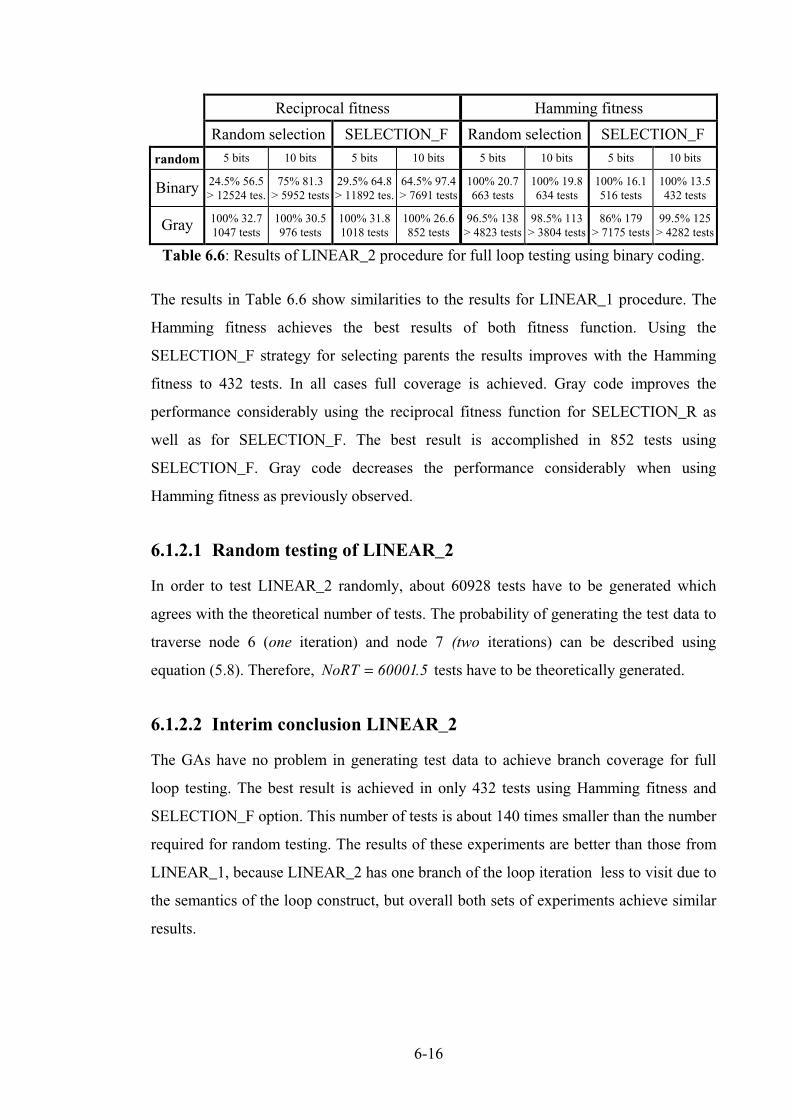
6-16
Table 6.6: Results of LINEAR_2 procedure for full loop testing using binary coding.
The results in Table 6.6 show similarities to the results for LINEAR_1 procedure. The
Hamming fitness achieves the best results of both fitness function. Using the
SELECTION_F strategy for selecting parents the results improves with the Hamming
fitness to 432 tests. In all cases full coverage is achieved. Gray code improves the
performance considerably using the reciprocal fitness function for SELECTION_R as
well as for SELECTION_F. The best result is accomplished in 852 tests using
SELECTION_F. Gray code decreases the performance considerably when using
Hamming fitness as previously observed.
6.1.2.1 Random testing of LINEAR_2
In order to test LINEAR_2 randomly, about 60928 tests have to be generated which
agrees with the theoretical number of tests. The probability of generating the test data to
traverse node 6 (one iteration) and node 7 (two iterations) can be described using
equation (5.8). Therefore, NoRT = 60001 5. tests have to be theoretically generated.
6.1.2.2 Interim conclusion LINEAR_2
The GAs have no problem in generating test data to achieve branch coverage for full
loop testing. The best result is achieved in only 432 tests using Hamming fitness and
SELECTION_F option. This number of tests is about 140 times smaller than the number
required for random testing. The results of these experiments are better than those from
LINEAR_1, because LINEAR_2 has one branch of the loop iteration less to visit due to
the semantics of the loop construct, but overall both sets of experiments achieve similar
results.
Reciprocal fitness Hamming fitness
Random selection SELECTION_F Random selection SELECTION_F
random 5 bits 10 bits 5 bits 10 bits 5 bits 10 bits 5 bits 10 bits
Binary 24.5% 56.5> 12524 tes.
75% 81.3> 5952 tests
29.5% 64.8> 11892 tes.
64.5% 97.4> 7691 tests
100% 20.7663 tests
100% 19.8634 tests
100% 16.1516 tests
100% 13.5432 tests
Gray 100% 32.71047 tests
100% 30.5976 tests
100% 31.81018 tests
100% 26.6852 tests
96.5% 138> 4823 tests
98.5% 113> 3804 tests
86% 179> 7175 tests
99.5% 125> 4282 tests

6-17
6.1.3 Binary Search
Often the search of an array is required whose elements are already arranged in order by
a key field. This fact can accelerate the search which is more efficient. This is an
advantage in that an array A of (1 .. N) is ordered such as to eliminate half of the array
elements with each probe into the array A. A suitable search algorithm is introduced
which makes use of this arrangement. Thus:
∀ ≤ ≤ ⋅ ≤−k k n A Ak k:Ζ 2 1 (6.1)
where Z is the set of all integers and k is a variable.
The basic idea of this algorithm, written as a function, is to check whether X (target key)
is equal to the middle element of an array section A(Mid). If so, X is found in the array A
and the search function returns the index of the array element and terminates.
If X is larger than A(Mid) it can be concluded that all elements with an index lower or
equal to MID can be excluded. This method is called binary search, because it will
eliminate, in each step, either the elements above or below the chosen try. If the key
element X is absent, an index value is returned which is one unit smaller than the first
index of the array in order to indicate that the key element is not present in the array.
Two index variables LOW and HIGH are used, which mark the left and the right end of
an array section, in which the required element may be found. The number of tries which
are necessary to search an array of the size N completely, directly depends on the
number of array elements. Therefore, the maximum number of comparisons is log ( )2 N
rounded to the next integer number. This algorithm is a huge improvement over the
linear search algorithm, where the average expected number of comparisons is N2 . The
control flow graph can be seen in Figure 6.8. The binary search function has 8 nodes 6
branches, two 'if' conditions and one 'while ... loop' statement. The peculiarity is the loop
condition which has besides the 'while' condition an extra second exit condition for the
loop which is realised by a 'return' statement in one of the 'if' conditions. This will
terminate and exit the loop when the target key matches one of the array elements.
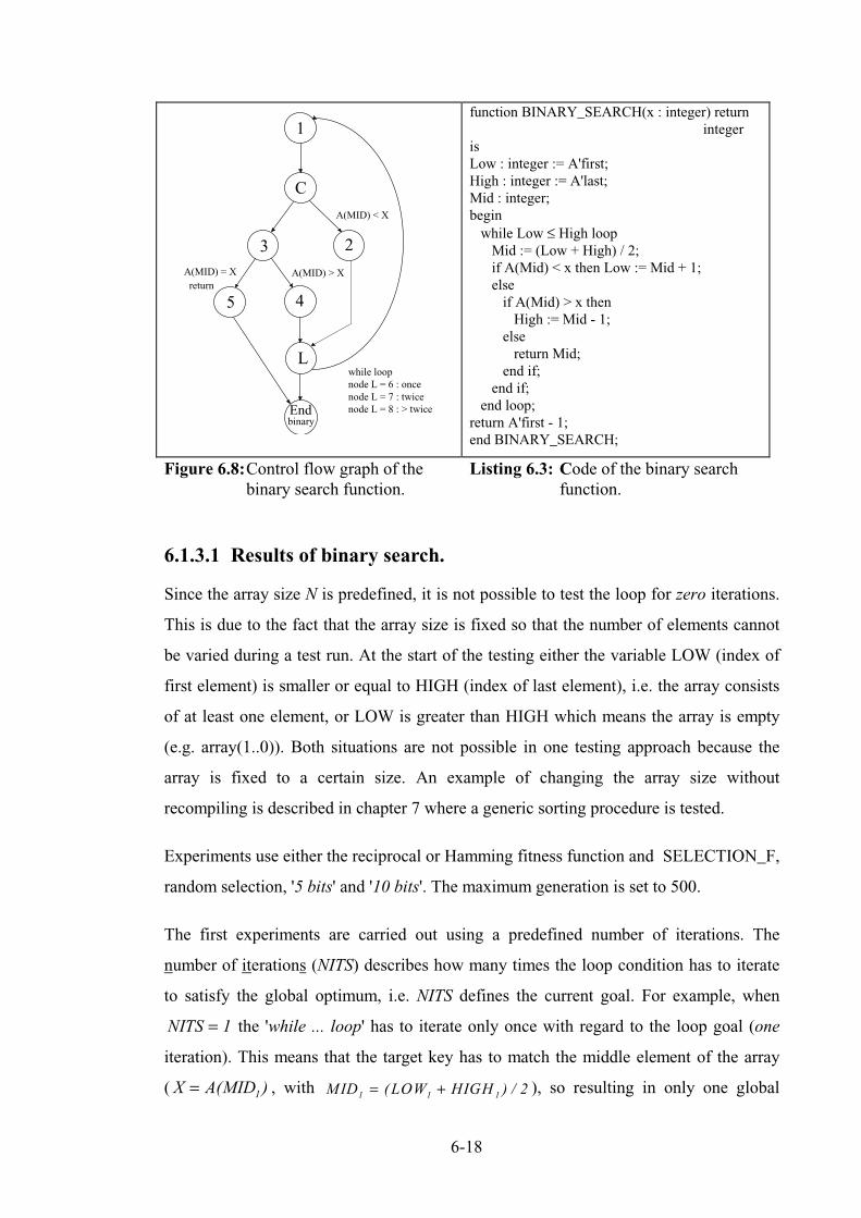
6-18
1
C
3 2
while loopnode L = 6 : oncenode L = 7 : twicenode L = 8 : > twice
L
5 4
A(MID) < X
End
A(MID) = X A(MID) > Xreturn
binary
function BINARY_SEARCH(x : integer) returninteger
isLow : integer := A'first;High : integer := A'last;Mid : integer;beginwhile Low ≤ High loopMid := (Low + High) / 2;if A(Mid) < x then Low := Mid + 1;elseif A(Mid) > x thenHigh := Mid - 1;
elsereturn Mid;
end if;end if;
end loop;return A'first - 1;end BINARY_SEARCH;
Figure 6.8:Control flow graph of thebinary search function.
Listing 6.3: Code of the binary searchfunction.
6.1.3.1 Results of binary search.
Since the array size N is predefined, it is not possible to test the loop for zero iterations.
This is due to the fact that the array size is fixed so that the number of elements cannot
be varied during a test run. At the start of the testing either the variable LOW (index of
first element) is smaller or equal to HIGH (index of last element), i.e. the array consists
of at least one element, or LOW is greater than HIGH which means the array is empty
(e.g. array(1..0)). Both situations are not possible in one testing approach because the
array is fixed to a certain size. An example of changing the array size without
recompiling is described in chapter 7 where a generic sorting procedure is tested.
Experiments use either the reciprocal or Hamming fitness function and SELECTION_F,
random selection, '5 bits' and '10 bits'. The maximum generation is set to 500.
The first experiments are carried out using a predefined number of iterations. The
number of iterations (NITS) describes how many times the loop condition has to iterate
to satisfy the global optimum, i.e. NITS defines the current goal. For example, when
NITS = 1 the 'while ... loop' has to iterate only once with regard to the loop goal (one
iteration). This means that the target key has to match the middle element of the array
( X A MID= ( )1 , with MID LOW HIGH1 1 1 2= +( ) / ), so resulting in only one global
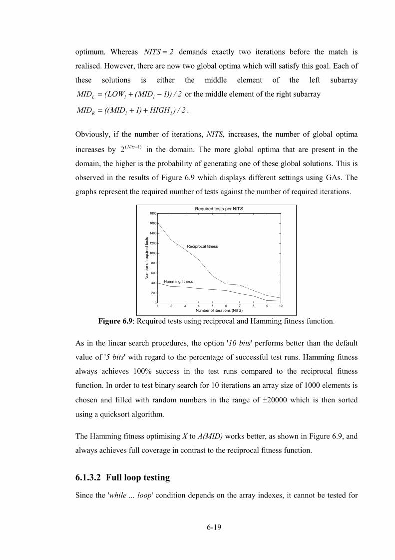
6-19
optimum. Whereas NITS = 2 demands exactly two iterations before the match is
realised. However, there are now two global optima which will satisfy this goal. Each of
these solutions is either the middle element of the left subarray
MID LOW MIDL = + −( ( )) /1 1 1 2 or the middle element of the right subarray
MID MID HIGHR = + +(( ) ) /1 11 2 .
Obviously, if the number of iterations, NITS, increases, the number of global optima
increases by 2 1)(Nits− in the domain. The more global optima that are present in the
domain, the higher is the probability of generating one of these global solutions. This is
observed in the results of Figure 6.9 which displays different settings using GAs. The
graphs represent the required number of tests against the number of required iterations.
1 2 3 4 5 6 7 8 9 100
200
400
600
800
1000
1200
1400
1600
1800
Number of iterations (NITS)
Num
berofrequiredtests
Required tests per NITS
Reciprocal fitness
Hamming fitness
Figure 6.9: Required tests using reciprocal and Hamming fitness function.
As in the linear search procedures, the option '10 bits' performs better than the default
value of '5 bits' with regard to the percentage of successful test runs. Hamming fitness
always achieves 100% success in the test runs compared to the reciprocal fitness
function. In order to test binary search for 10 iterations an array size of 1000 elements is
chosen and filled with random numbers in the range of ±20000 which is then sorted
using a quicksort algorithm.
The Hamming fitness optimising X to A(MID) works better, as shown in Figure 6.9, and
always achieves full coverage in contrast to the reciprocal fitness function.
6.1.3.2 Full loop testing
Since the 'while ... loop' condition depends on the array indexes, it cannot be tested for
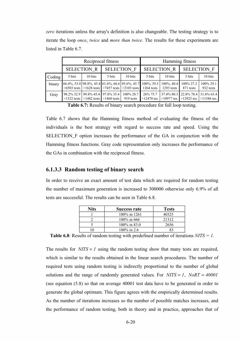
6-20
zero iterations unless the array's definition is also changeable. The testing strategy is to
iterate the loop once, twice and more than twice. The results for these experiments are
listed in Table 6.7.
Table 6.7: Results of binary search procedure for full loop testing.
Table 6.7 shows that the Hamming fitness method of evaluating the fitness of the
individuals is the best strategy with regard to success rate and speed. Using the
SELECTION_F option increases the performance of the GA in conjunction with the
Hamming fitness functions. Gray code representation only increases the performance of
the GAs in combination with the reciprocal fitness.
6.1.3.3 Random testing of binary search
In order to receive an exact amount of test data which are required for random testing
the number of maximum generation is increased to 300000 otherwise only 6.9% of all
tests are successful. The results can be seen in Table 6.8.
Table 6.8: Results of random testing with predefined number of iterations NITS = 1.
The results for NITS = 1 using the random testing show that many tests are required,
which is similar to the results obtained in the linear search procedures. The number of
required tests using random testing is indirectly proportional to the number of global
solutions and the range of randomly generated values. For NITS = 1, NoRT = 40001
(see equation (5.8) so that on average 40001 test data have to be generated in order to
generate the global optimum. This figure agrees with the empirically determined results.
As the number of iterations increases so the number of possible matches increases, and
the performance of random testing, both in theory and in practice, approaches that of
Reciprocal fitness Hamming fitness
SELECTION_R SELECTION_F SELECTION_R SELECTION_F
Coding 5 bits 10 bits 5 bits 10 bits 5 bits 10 bits 5 bits 10 bits
binary 66.4%, 53.0>6503 tests
98.8%, 45.4>1628 tests
61.6%, 66.6>7457 tests
95.6%, 45.7>2103 tests
100%, 39.51264 tests
100%, 40.41293 tests
100% 27.2871 tests
100% 29.1932 tests
Gray 98.2% 32.9>1322 tests
99.8% 45.4>1482 tests
97.8% 35.4>1460 tests
100% 28.7919 tests
26% 75.7>12470 tes.
37.4% 80.3>10977 tes.
22.8% 78.4>12925 tes.
31.6% 63.4>11586 tes.
Nits Success rate Tests1 100% in 1261 403252 100% in 666 213125 100% in 83.0 265610 100% in 2.6 83

6-21
GAs. This is because the cardinality of the required sub-domain increases. When
NITS = 10 there are 512 global solutions which require 79 tests, on average until one of
the global solutions is generated. For full loop testing about 48640 tests are required
compared to only 871 tests achieved with GA. The theoretical number of random tests
using equation (5.8) is NoRT = 50002 .
6.1.4 Using character in LINEAR_1 and BINARY_SEARCH
In all previous test procedures the global optima are based on integer array data types. In
this section a character data type is used. The character data type is converted for the
evaluation of the fitness either, into its corresponding ASCII value (if the reciprocal
fitness function is used) or immediately into a binary string in the case of using
Hamming fitness function.
The GAs have no problems in generating test data to traverse all nodes. For the linear
search and the binary search, the GA performed better than in pure random testing. The
LINEAR_1 search procedure achieves 100% success in only 7.0 generations for one
iteration (binary search required 7.1 generations). This corresponds to 56 tests, since a
character consists of eight bits, so the population size PSZ has correspondingly only 8
individuals. For the full loop testing about 8.7 generations are required. Using the
LINEAR_1 procedure, random testing achieves 100% in 83 tests for zero iterations and
for full testing criteria the number of required generations increases to 198 tests.
The last experiment using the search procedure LINEAR_1 is carried out with a new
data type. A string of four characters (array of four characters) is used in order to
generate test data for full loop testing. The string of characters is handled as a one bit
string. Considerably more test data are required in order to satisfy all branch conditions
for full iteration testing since the input domain has a size of 1274 and only three
solutions exist (global optima) to iterate the loop zero, one and two times. About 93.2
generations are needed to generate test data (100% success rate) which execute all
branches, where the number of individuals per generation has increased from 8
(character size) to 32 bits (PSZ = four times the character size). Random testing is not
feasible for all available characters (ASCII code from 1 to 127) because of the amount of
test data which have to be produced. Theoretically 1274 possible combinations exist, i.e.
for one iteration X = A(1). This means on average 1274 test data have to be generated in

6-22
order to traverse the iterations once. This would take too long a period of time.
6.1.4.1 Conclusion of search procedures
One of the problems which occurrs during the use of the reciprocal fitness function is
that it is difficult for the GA to optimise towards large values. This is observed in the
first and second set of experiments using LINEAR_1 where a value of 10000 or random
numbers are used for the first element of the array A, whereas it achieves good results
when global optima represent small values. The reason for this lies in the nature of the
reciprocal fitness function which favours smaller values. This is reflected in the results
of the quadratic and triangle procedures, which favours smaller values for their input
variables to generate global solutions. This is expressed by the increased number of zero
solutions generated in the quadratic equation solver program.
Although the GA rapidly finds an area with a global optimum, the GA will not locate the
global optimum with the same kind of speed, DeJong [1993] and Figure 6.2 and Figure
6.4. Therefore, the idea of the weighted mutation is to undertake a local search to speed
up the finding of the global optimum, when the population seems not to improve
anymore, and thereby endeavouring to overcome local optima. If the GA tries to
optimise towards the value of 10000, a possible local optimum could be 9983 which is
in binary code 1111111101100100. Just by changing only one bit of the bit string, the
quality of the test data will diminish because the test data moves further away from the
optimum. If bits is restricted to the last five bits of the bit string, the weighted mutation
operator cannot do anything to improve the fitness (using reciprocal fitness function) of
the test data because the last 8 significant bits are already set to 1 and changing them to
0 decreases the numeric value and so the fitness. Increasing the parameter value bits to
'10 bits', or using Gray code in the case of the reciprocal fitness function could reduce
this trap as shown in the results of the search procedures. The advantage of the
Hamming fitness function is that it compares the bit pattern and not the numeric values.
If the loop conditions are thoroughly tested, the testing for more than two iterations is
usually done instantly which means the GA or the random testing do not have to spend
much time on that special branch in order to execute it. Using Hamming fitness is more
consistent than the reciprocal fitness function. In conjunction with SELECTION_F it is
always faster in generating global solutions.

6-23
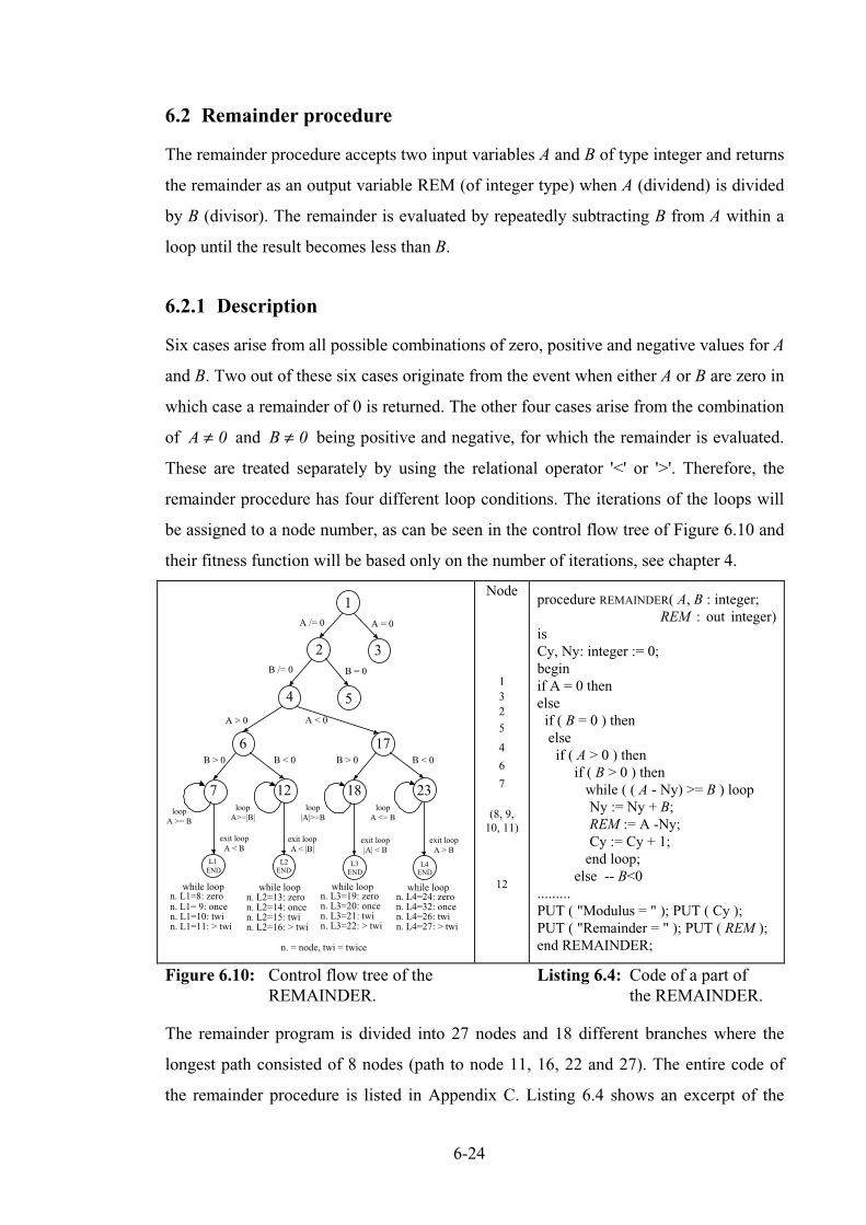
6-24
6.2 Remainder procedure
The remainder procedure accepts two input variables A and B of type integer and returns
the remainder as an output variable REM (of integer type) when A (dividend) is divided
by B (divisor). The remainder is evaluated by repeatedly subtracting B from A within a
loop until the result becomes less than B.
6.2.1 Description
Six cases arise from all possible combinations of zero, positive and negative values for A
and B. Two out of these six cases originate from the event when either A or B are zero in
which case a remainder of 0 is returned. The other four cases arise from the combination
of A ≠ 0 and B ≠ 0 being positive and negative, for which the remainder is evaluated.
These are treated separately by using the relational operator '<' or '>'. Therefore, the
remainder procedure has four different loop conditions. The iterations of the loops will
be assigned to a node number, as can be seen in the control flow tree of Figure 6.10 and
their fitness function will be based only on the number of iterations, see chapter 4.
1
2
4
6
3
5
17
A = 0A /= 0
B /= 0 B = 0
A > 0 A < 0
B > 0 B < 0
loopA >= B
loopA <= B
B < 0B > 0
7 12 18
END
exit loopA < B
exit loopA < |B|
loop|A|>=B
loopA>=|B|
exit loop|A| < B
exit loopA > B
23
while loopn. L1=8: zeron. L1= 9: oncen. L1=10: twin. L1=11: > twi
while loopn. L2=13: zeron. L2=14: oncen. L2=15: twin. L2=16: > twi
while loopn. L4=24: zeron. L4=32: oncen. L4=26: twin. L4=27: > twi
while loopn. L3=19: zeron. L3=20: oncen. L3=21: twin. L3=22: > twi
END END END
L1 L2 L3 L4
n. = node, twi = twice
Node
132
5
4
6
7
(8, 9,10, 11)
12
procedure REMAINDER( A, B : integer;REM : out integer)
isCy, Ny: integer := 0;beginif A = 0 thenelseif ( B = 0 ) thenelseif ( A > 0 ) then
if ( B > 0 ) thenwhile ( ( A - Ny) >= B ) loopNy := Ny + B;REM := A -Ny;Cy := Cy + 1;end loop;
else -- B<0.........PUT ( "Modulus = " ); PUT ( Cy );PUT ( "Remainder = " ); PUT ( REM );end REMAINDER;
Figure 6.10: Control flow tree of theREMAINDER.
Listing 6.4: Code of a part ofthe REMAINDER.
The remainder program is divided into 27 nodes and 18 different branches where the
longest path consisted of 8 nodes (path to node 11, 16, 22 and 27). The entire code of
the remainder procedure is listed in Appendix C. Listing 6.4 shows an excerpt of the

6-25
code of the REMAINDER procedure covering the path to the first loop conditions (path:
1, 2, 4, 6, 7, 8 or 9 or 10 or 11 ), i.e. A positive and B negative.
6.2.2 Results of Remainder
In these experiments, the two variables A and B are to be optimised by the GA, therefore
the population has Psz = 64 members and the mutation probability is Pm = 0 016. , since
P PmSC
= 1 .
Two of the branches (node 3 and node 5 seen in Figure 6.10) have the lowest probability
of being traversed because these branches filter the cases when A = 0 or B = 0 . This
means that there is only one global solution for each of these nodes. These branches are
only traversed if test data are generated for A and B which have the value of 0.
Assuming that the input range is between ± 20000, the probability for each branch
having been traversed is P3 551
400012 5 10, .= = ⋅ − . This reflects the high number of tests
required to be performed for random testing to achieve full branch coverage. The test
data are checked using a post condition which is the Ada function REM.
Results of the experiments are shown in Table 6.9 where MAX_GENERATION is set to
200.
Table 6.9: Results for full loop testing using REMAINDER.
Reciprocal and Hamming fitness functions achieves similar results when random
selection is chosen. However, SELECTION_F improves the performance using
Hamming fitness by about 5 generations and full branch coverage is nearly always
achieved. The reciprocal fitness results deteriorate to about only 86% to 95% success
rate. The nodes 3 and 5 are not responsible for the decrease in performance, as expected.
The problem nodes are the iteration nodes which have many global optima, so that the
Reciprocal fitness Hamming fitness
SELECTION_R SELECTION_F SELECTION_R SELECTION_F
Coding 5 bits 10 bits 5 bits 10 bits 5 bits 10 bits 5 bits 10 bits
binary 100% 15.2973 tests
100% 14.7944 tests
86% 12.92502 tests
95.5% 11.41273 tests
100% 15.2974 tests
100% 15.5959 tests
98% 10.9937 tests
100% 10.1644 tests
Gray 100% 22.91463 tests
100% 20.31297 tests
87.5% 22.62863 tests
97% 19.81616 tests
72% 39.35416 tests
92% 33.73010 tests
49% 38.77741 tests
84% 38.44115 tests
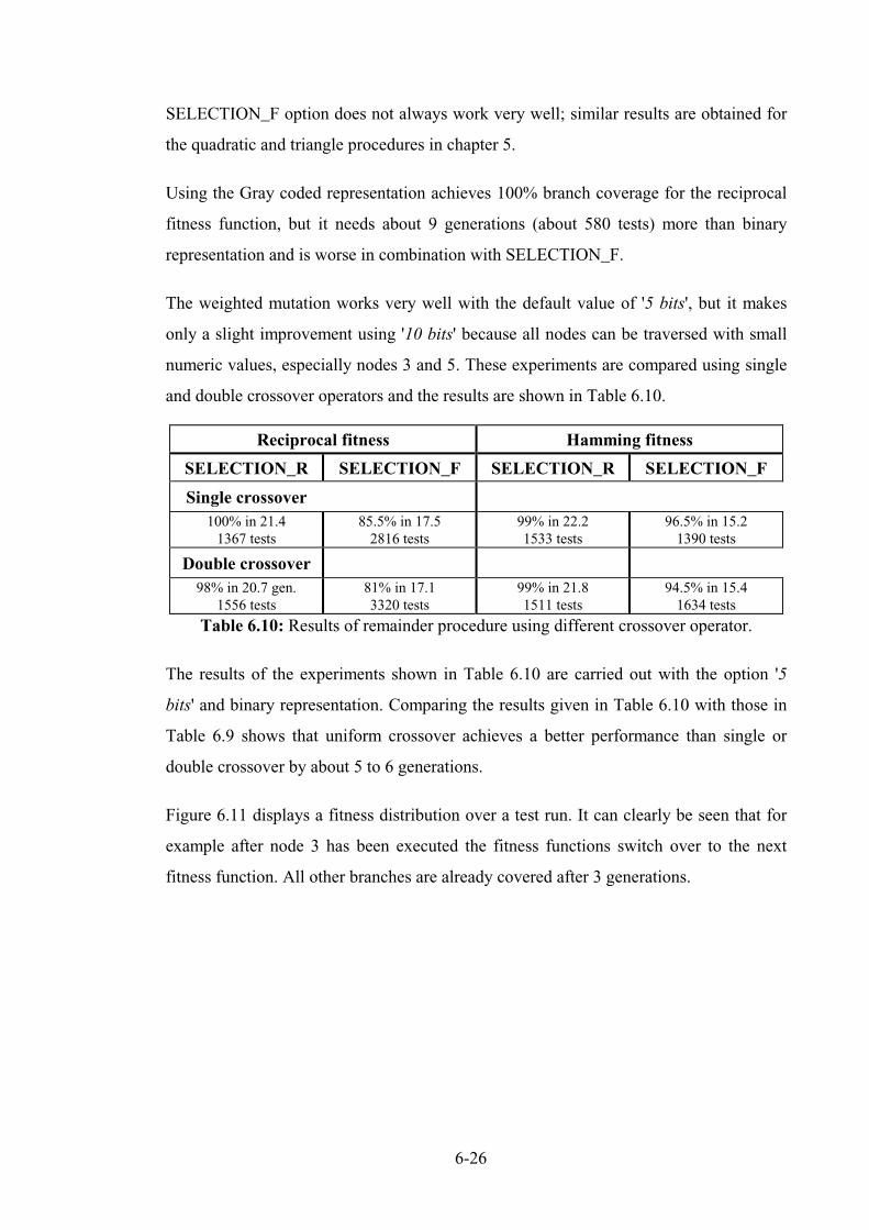
6-26
SELECTION_F option does not always work very well; similar results are obtained for
the quadratic and triangle procedures in chapter 5.
Using the Gray coded representation achieves 100% branch coverage for the reciprocal
fitness function, but it needs about 9 generations (about 580 tests) more than binary
representation and is worse in combination with SELECTION_F.
The weighted mutation works very well with the default value of '5 bits', but it makes
only a slight improvement using '10 bits' because all nodes can be traversed with small
numeric values, especially nodes 3 and 5. These experiments are compared using single
and double crossover operators and the results are shown in Table 6.10.
Table 6.10: Results of remainder procedure using different crossover operator.
The results of the experiments shown in Table 6.10 are carried out with the option '5
bits' and binary representation. Comparing the results given in Table 6.10 with those in
Table 6.9 shows that uniform crossover achieves a better performance than single or
double crossover by about 5 to 6 generations.
Figure 6.11 displays a fitness distribution over a test run. It can clearly be seen that for
example after node 3 has been executed the fitness functions switch over to the next
fitness function. All other branches are already covered after 3 generations.
Reciprocal fitness Hamming fitness
SELECTION_R SELECTION_F SELECTION_R SELECTION_F
Single crossover100% in 21.41367 tests
85.5% in 17.52816 tests
99% in 22.21533 tests
96.5% in 15.21390 tests
Double crossover98% in 20.7 gen.
1556 tests81% in 17.13320 tests
99% in 21.81511 tests
94.5% in 15.41634 tests
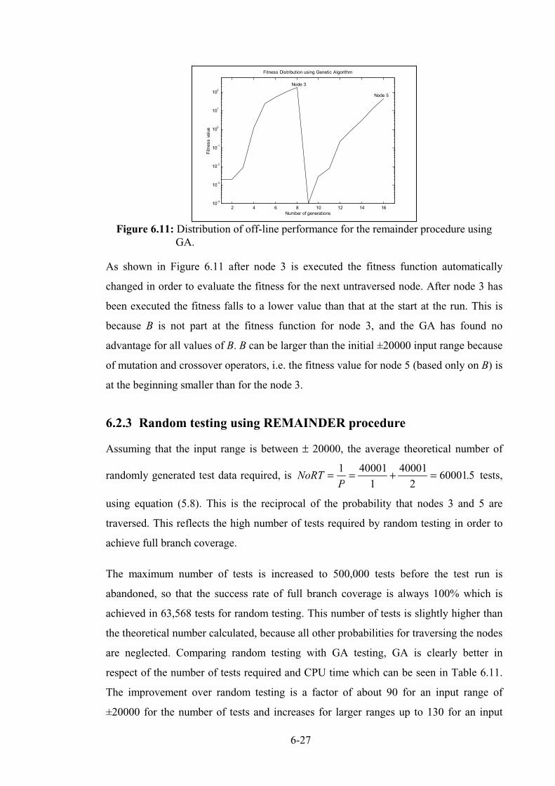
6-27
2 4 6 8 10 12 14 1610-4
10-3
10-2
10-1
100
101
102
Number of generationsFitnessvalue
Fitness Distribution using Genetic Algorithm
Node 3
Node 5
Figure 6.11: Distribution of off-line performance for the remainder procedure usingGA.
As shown in Figure 6.11 after node 3 is executed the fitness function automatically
changed in order to evaluate the fitness for the next untraversed node. After node 3 has
been executed the fitness falls to a lower value than that at the start at the run. This is
because B is not part at the fitness function for node 3, and the GA has found no
advantage for all values of B. B can be larger than the initial ±20000 input range because
of mutation and crossover operators, i.e. the fitness value for node 5 (based only on B) is
at the beginning smaller than for the node 3.
6.2.3 Random testing using REMAINDER procedure
Assuming that the input range is between ± 20000, the average theoretical number of
randomly generated test data required, is NoRTP
= = + =1 400011
400012
600015. tests,
using equation (5.8). This is the reciprocal of the probability that nodes 3 and 5 are
traversed. This reflects the high number of tests required by random testing in order to
achieve full branch coverage.
The maximum number of tests is increased to 500,000 tests before the test run is
abandoned, so that the success rate of full branch coverage is always 100% which is
achieved in 63,568 tests for random testing. This number of tests is slightly higher than
the theoretical number calculated, because all other probabilities for traversing the nodes
are neglected. Comparing random testing with GA testing, GA is clearly better in
respect of the number of tests required and CPU time which can be seen in Table 6.11.
The improvement over random testing is a factor of about 90 for an input range of
±20000 for the number of tests and increases for larger ranges up to 130 for an input
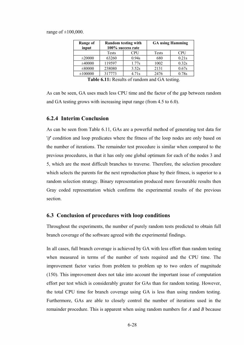
6-28
range of ±100,000.
Table 6.11: Results of random and GA testing.
As can be seen, GA uses much less CPU time and the factor of the gap between random
and GA testing grows with increasing input range (from 4.5 to 6.0).
6.2.4 Interim Conclusion
As can be seen from Table 6.11, GAs are a powerful method of generating test data for
'if' condition and loop predicates where the fitness of the loop nodes are only based on
the number of iterations. The remainder test procedure is similar when compared to the
previous procedures, in that it has only one global optimum for each of the nodes 3 and
5, which are the most difficult branches to traverse. Therefore, the selection procedure
which selects the parents for the next reproduction phase by their fitness, is superior to a
random selection strategy. Binary representation produced more favourable results then
Gray coded representation which confirms the experimental results of the previous
section.
6.3 Conclusion of procedures with loop conditions
Throughout the experiments, the number of purely random tests predicted to obtain full
branch coverage of the software agreed with the experimental findings.
In all cases, full branch coverage is achieved by GA with less effort than random testing
when measured in terms of the number of tests required and the CPU time. The
improvement factor varies from problem to problem up to two orders of magnitude
(150). This improvement does not take into account the important issue of computation
effort per test which is considerably greater for GAs than for random testing. However,
the total CPU time for branch coverage using GA is less than using random testing.
Furthermore, GAs are able to closely control the number of iterations used in the
remainder procedure. This is apparent when using random numbers for A and B because
Range ofinput
Random testing with100% success rate
GA using Hamming
Tests CPU Tests CPU±20000 63260 0.94s 680 0.21s±40000 119597 1.77s 1002 0.32s±80000 238080 3.52s 2131 0.67s±100000 317773 4.71s 2476 0.78s
6-29
if these input variables have very different values, the loop will iterate many times
which costs a lot of CPU time, whereas GAs try to control these variables so that the
number of iterations are reduced.
In this instance, the SELECTION_F option of selecting parents for reproduction by their
fitness values is better than random selection. The reason for this result is that in all
search procedures, specially in the linear search procedures, there is only one global
optimum per node so that there is no confusion regarding different goals per node. In the
remainder procedure, the fitness for executing the loops is based solely on the number of
iterations required. This provides a straight forward way of controlling the loops.
However, in linear and binary search procedures, this approach causes problems, since
the array element values are not continuous, especially in the case of the linear search
where the values of the array elements are not sorted. Therefore, the array elements,
which are used as the predicate condition in the 'while ... loop' (LINEAR_1), 'loop ...
exit' (LINEAR_2) and in the 'while ... loop ... return' (binary search) are needed as the
base for the fitness functions. The binary search procedure is in one sense an exception
because of the construction of the loop condition which has one condition in the 'while
...' statement and a second condition is involved in nested 'if' condition with a 'return'
command which terminates the loop as soon it is executed.
The results of these experiments confirm several hypotheses and clarify them in more
detail. Hypothesis 1 is confirmed by the much more efficient behaviour of GAs. The
standard setting (hypothesis 2) has been made more precise for different features. Gray
code is normally better with a reciprocal fitness function than using binary code
(hypothesis 2_1) which is better in combination with Hamming fitness function. If only
few global optima exists, it is better to use selection according to fitness, if there are
several, use random selection (hypothesis 2_2). Hypothesis 2_3 is confirmed again that
uniform crossover is superior. Hypothesis 2_4 is justified by using different population
sizes and the best is found as stated in the hypothesis. The hypothesis 3 which is under
close investigation in this chapter is confirmed by generating test data for the different
number of loop iterations.
In the next chapter commercially available software is used as the procedure under test,
which has more complex data types.
7-1
CHAPTER 7
Testing generic procedure
In previous chapters, test data have been generated automatically for various procedures.
These include a quadratic equation solver, a system of five procedures for classifying
triangles, remainder calculation procedure and linear and binary search procedures. The
quadratic equation solver and the triangle procedures contain 'if' conditions and the other
procedures in addition have various loop conditions. The performance of the GAs with
regard to these procedures is undoubtedly better than pure random testing which need up
to more than two orders of magnitude more tests to achieve full branch coverage.
The aim of this chapter is to investigate and characterise the behaviour of a generic
procedure and its implementation and effect. A generic sorting procedure is used which
has more complicated data structure such as records.
7.1 Generic Sorting Procedure: Direct Sort
The procedure DIRECT_SORT is commercially available and is tested as supplied. The
purpose of the procedure is to sort an array of elements in the main memory into
ascending order; it is based on the quicksort algorithm which partitions the array and
swaps low values in the upper partition with high values in the lower partition. The out-
of-order values move large distances which leads to efficient sorting under favourable
circumstances. It is considerably more complicated than many of the other procedures
because:
• it is generic,
• it contains two local procedures (INSERT and PARTITION), and
• procedure PARTITION has its own local procedure SWAP.
Overall, DIRECT_SORT consist of six loops and eight selections several of which are
nested. The control flow graphs of the procedures MAIN, PARTITION, INSERT and
SWAP are shown in Figure 7.1, Figure 7.2, Figure 7.3 and Figure 7.4 respectively and
the Ada code for these procedures is in Appendix D.

7-2
The symbol C in a node means that this is a decision node with no extra node number
Main
2
10
8
3
9
exit loop
14
loop exitnode L1=11: oncenode L1=12: twicenode L1=13: > twiceINSERT
Partition
4 5
t f
t f
ENDMain
L1
ft
t f
6
C
7
PARTITION
24 25
30
L2
39
exitwhile loop
END
f
exit loop
26 27
28 29
while loopnode L2=31: zeronode L2=32: oncenode L2=33: twicenode L2=34: > twice
while loopnode L3=35: zeronode L3=36: oncenode L3=37: twicenode L3=38: > twice
exitwhile loop
40
loop exitnode L4=41: oncenode L4=42: twicenode L4=43: > twice
t
L4
f
t f
ft
C
C
C
L3t
SWAP
SWAP
SWAP
Partition
Figure 7.1: Control flow graph ofDIRECT_SORT.
Figure 7.2: Control flow graph ofprocedure PARTITION.
INSERT
L5
15
C
L6
exitfor loop
exitwhile loop
while loopnode L5=16: zeronode L5=17: oncenode L5=18: twicenode L5=19: > twice
for loopnode L6=20: zeronode L6=21: oncenode L6=22: twicenode L6=23: > twice
ENDL6 SWAP
44
ENDSwap
Figure 7.3:Control flow graph ofprocedure INSERT.
Figure 7.4: Control flow graph ofprocedure SWAP.
7-3
7.2 Generic feature
Since DIRECT_SORT is written as a generic package (see chapter 5), it has to be
instantiated in the main program. The generic package header of the sorting procedure
is:
1. type index_type is (<>);
2. type scalar_type is private;
3. type vector_type is array(index_type range <>) of scalar_type;
4. with function LT (a, b: in scalar_type) return boolean;
This generic section at the head of the DIRECT_SORT package allows different data
types to be sorted by instantiation of those generic types, Barnes [1984], without
recompiling the source code. The first statement of the generic section defined the
index_type to be any discrete type, (<>), which could declare the indices of an array to
be sorted. The array type elements can be defined as being of any type and is
instantiated into the scalar_type. The third statement declares the array type to be sorted
in terms of a limited range of index_type and scalar_type. In order to define the ordering
of the elements in a sorting procedure, it is essential that the user defines a 'Less-Than'
function (LT) for variables of scalar_type (fourth statement). This has to be done
because the 'Less-Than' operators, i.e. '<' or '>' are only defined for primitive data types.
The program which calls the generic DIRECT_SORT has, therefore, to declare
appropriate types for index_type, scalar_type and vector_type as well as an appropriate
function definition for LT. These are then used to instantiate the sort package.
Due to the increased complexity and expected usage, (valid for all possible data types),
of DIRECT_SORT, and the combined instantiation of the package, the testing of such
generic procedure needs to be more thorough than normal, even though the Ada
compiler is very precise in type checking.
Generic procedures may contain more complex 'if' and 'loop' conditions than
encountered previously, and this is reflected in an increased complexity of testing. This
is due to the fact that some conditions relate to the definition of the discrete types which
are instantiated into the generic package. One example of this is the condition for
checking the indexes of the array where top is equivalent to UPPER and bottom to
LOWER:

7-4
if (index_type'pos(top) < index_type'pos(bottom) ) then...
This tests the index_type to see whether the top array index is smaller than the bottom
index, as allowed by the Ada compiler. If this is the case, the array is empty (Ada83
LRM, 3.6.1 [1983]) and DIRECT_SORT returns an error flag and terminates the
sorting.
Another test case checks the size of index_type (number of elements to be sorted) in
order to ascertain whether the array section is of sufficient length to make partitioning
worth while. The condition is of the form:
if index_type'pos(right) - index_type'pos(left) > 10 then...
If the condition is true, the array will be partitioned and sorted by the procedure
PARTITION and the local procedure SWAP. In the case of an array size smaller than 10
elements the array is sorted by the procedure INSERT. Such conditions have to be tested
and can be difficult to check manually, because of the complexity of the conditions.
The size of the array has to vary in order to test the second condition. This can make
things difficult since the GAs normally use a fixed length number of bits for the
chromosomes. A strategy, therefore, has to be found to compensate for this phenomenon
as described in the next section, Sthamer [1994].
7.3 Test strategy and data structure
The first experiments are carried out using the normal method of implementing the
instrumentation procedures (see chapter 3), into the procedure under test. On feeding
test data, in this case arrays, into the DIRECT_SORT procedure, the array elements
should be sorted into ascending order on completion of the procedure. The original test
data is then fed into a different quicksort procedure to verify the functionality of
DIRECT_SORT.
For the first experiments the array size is restricted and fixed to 10 elements and the data
type is an array of integers. The result is unsatisfactory although the testing tool
traversed all possible branches within this set-up. The problem is identified as the
definition of the array's set-up. Since the array is fixed in this first experiment and the
size is limited to 10 elements, it is not possible to execute those branches which

7-5
involved the size of the array. In total only twelve nodes are executed. These are nodes
3, 4, 6, 10, 11, 14, 15, 16, 17, 18, 19 and 23. All other branches could not be executed.
Branches 3 and 4 are executed because the top index of the array (index_type) is always
larger than the bottom index ( 10 > 1), therefore nodes 2 and 5 could not have been
executed. Since the array is fixed to ten elements, node 10 can only be executed which is
directly related to the size of the array. Node 11 is executed which is a loop condition
for one iteration. The loop can only be executed once as long as the array consists of less
than 11 elements. Nodes 15, 16, 17, 18 and 19 are executed because they do not relate to
the array size or the values of the array indices. They belong to a loop condition in the
procedure INSERT. Node 23 belong to a 'for ... loop' condition with more than two
iterations. Zero, one and two iterations (node 20, 21 and 22) are not traversed because
they relate directly to various sizes of the array. Zero iterations could only be fulfilled
when top index minus bottom index is zero (one array element), one iteration is
performed if the difference is one, etc.
The next experiment carried out, uses an array size of 12 elements. Compared to the
previous experiment more nodes are executed in total, but full branch coverage is not
achieved. Node 2 is not executed because the size of the array is still fixed at 12
elements since upper'index_type (12) is always larger than lower'index_type (1). In order
to traverse nodes 20, 21 and 22, the index_type ought to be variable as explained above.
All those untraversed nodes relate to the main condition that the index_type (array size)
is fixed and not a variable. The structure of the testing tool requires altering so that the
sizes of the array could change. This is achieved by varying the size of the actual
chromosomes. Although the length of the active part of the chromosome of the array is
altered, it is still fixed to a certain size. However, the size of the index_type which
defines the array size to be sorted (test data) will be made variable within a certain
range. In order to make the index_type variable two extra variables, (LOWER and
UPPER) of type integer, are incorporated into the structure of the chromosome so that
these two variables can also be influenced by the GA. It is decided that the maximum
size of the array should be restricted to 16 array elements. The choice is now whether to
use the entire array or just a part of it. The maximum size of 16 elements is chosen
because of the computational effort in the case of a larger array. The size of 16 elements
is also convenient in that it can be represented with four bits between 0 and 15. The
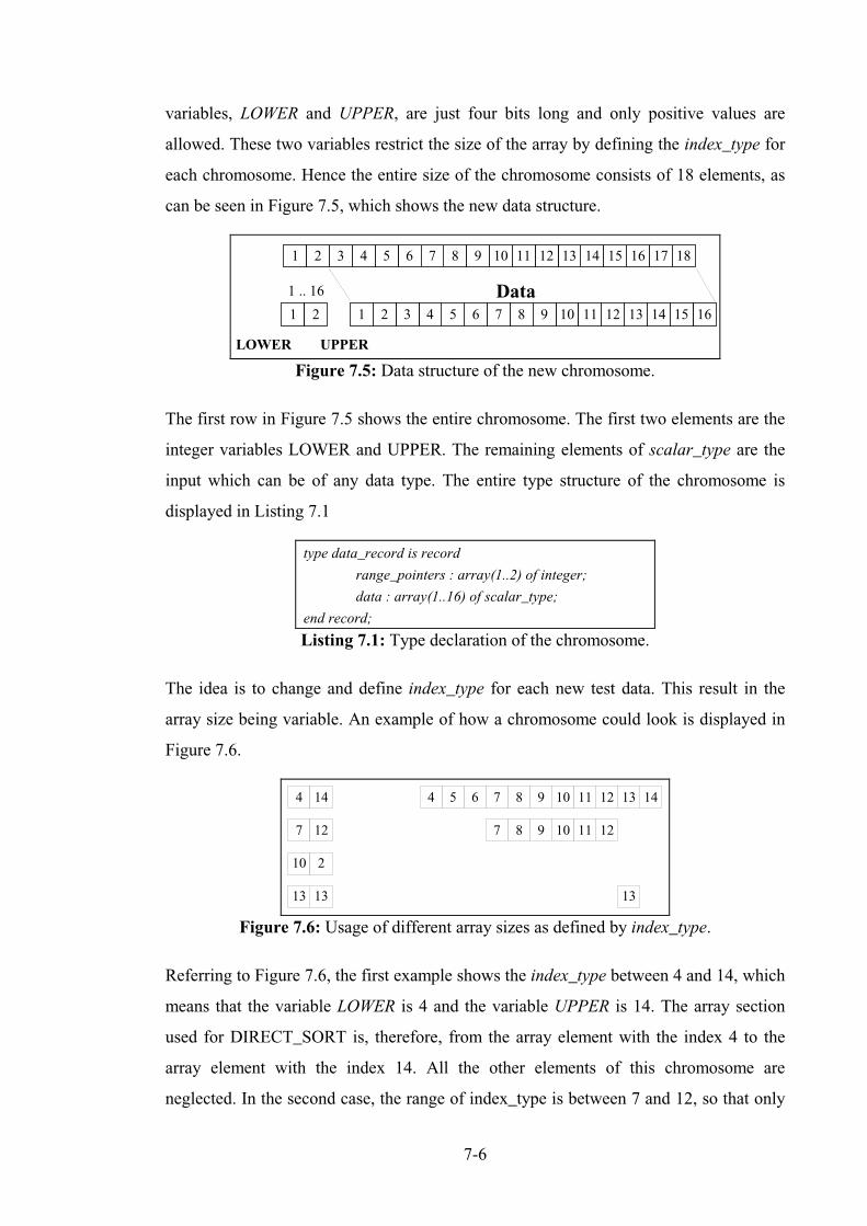
7-6
variables, LOWER and UPPER, are just four bits long and only positive values are
allowed. These two variables restrict the size of the array by defining the index_type for
each chromosome. Hence the entire size of the chromosome consists of 18 elements, as
can be seen in Figure 7.5, which shows the new data structure.
1 .. 16 Data1 65432 14131287
17
1615109 11
181 65432 14131287 1615109 11
1 2
LOWER UPPER
Figure 7.5: Data structure of the new chromosome.
The first row in Figure 7.5 shows the entire chromosome. The first two elements are the
integer variables LOWER and UPPER. The remaining elements of scalar_type are the
input which can be of any data type. The entire type structure of the chromosome is
displayed in Listing 7.1
Listing 7.1: Type declaration of the chromosome.
The idea is to change and define index_type for each new test data. This result in the
array size being variable. An example of how a chromosome could look is displayed in
Figure 7.6.
654 14131287 109 11
1287 109 11
13
4 14
7 12
1313
10 2
Figure 7.6: Usage of different array sizes as defined by index_type.
Referring to Figure 7.6, the first example shows the index_type between 4 and 14, which
means that the variable LOWER is 4 and the variable UPPER is 14. The array section
used for DIRECT_SORT is, therefore, from the array element with the index 4 to the
array element with the index 14. All the other elements of this chromosome are
neglected. In the second case, the range of index_type is between 7 and 12, so that only
type data_record is record
range_pointers : array(1..2) of integer;
data : array(1..16) of scalar_type;
end record;
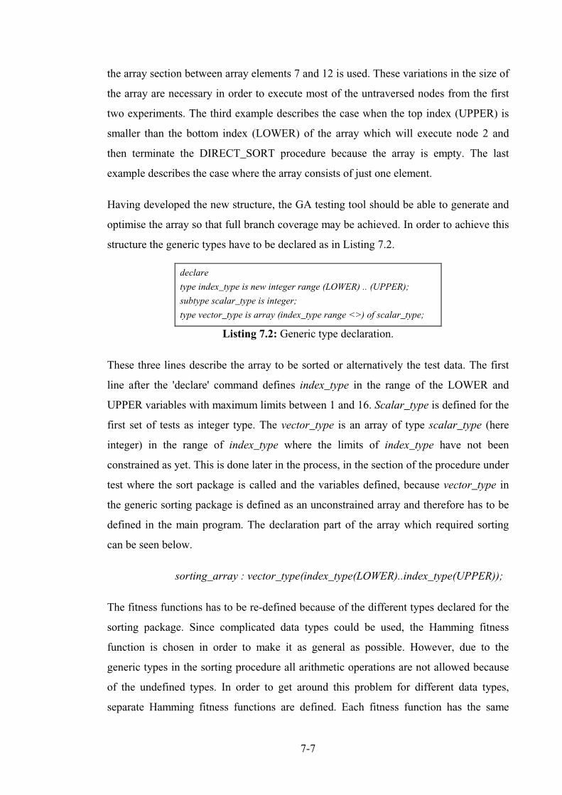
7-7
the array section between array elements 7 and 12 is used. These variations in the size of
the array are necessary in order to execute most of the untraversed nodes from the first
two experiments. The third example describes the case when the top index (UPPER) is
smaller than the bottom index (LOWER) of the array which will execute node 2 and
then terminate the DIRECT_SORT procedure because the array is empty. The last
example describes the case where the array consists of just one element.
Having developed the new structure, the GA testing tool should be able to generate and
optimise the array so that full branch coverage may be achieved. In order to achieve this
structure the generic types have to be declared as in Listing 7.2.
Listing 7.2: Generic type declaration.
These three lines describe the array to be sorted or alternatively the test data. The first
line after the 'declare' command defines index_type in the range of the LOWER and
UPPER variables with maximum limits between 1 and 16. Scalar_type is defined for the
first set of tests as integer type. The vector_type is an array of type scalar_type (here
integer) in the range of index_type where the limits of index_type have not been
constrained as yet. This is done later in the process, in the section of the procedure under
test where the sort package is called and the variables defined, because vector_type in
the generic sorting package is defined as an unconstrained array and therefore has to be
defined in the main program. The declaration part of the array which required sorting
can be seen below.
sorting_array : vector_type(index_type(LOWER)..index_type(UPPER));
The fitness functions has to be re-defined because of the different types declared for the
sorting package. Since complicated data types could be used, the Hamming fitness
function is chosen in order to make it as general as possible. However, due to the
generic types in the sorting procedure all arithmetic operations are not allowed because
of the undefined types. In order to get around this problem for different data types,
separate Hamming fitness functions are defined. Each fitness function has the same
declare
type index_type is new integer range (LOWER) .. (UPPER);
subtype scalar_type is integer;
type vector_type is array (index_type range <>) of scalar_type;

7-8
structure and deals with index_types, scalar_types or integer types.
7.4 Different Tests
Experiments are carried out with different scalar_types, such as integer, records with
fields of type integer and character, and also where the fields are in reverse order. The
key in each of these is the first data type. If the second data type is chosen as the key, the
same results would have been produced.
Different experiments are carried out without changing the MSB in the weighted
mutation operator when integers or records (of integer and character) are chosen as the
scalar_type. Another set of experiments deals with disabling the CONTROL_PARENT
procedure which converts the two's complement (produced by the conversion for
negative numeric values) into a binary representation where the MSB is the sign bit. If a
record is considered as a one bit string, no direct access to the MSB is possible in a
single bit string which is explained in Figure 7.7.
exploded data integer
char
recordintegercharacter
1 32 40
1 8
1 32
Figure 7.7: Example of a chromosome using different data types.
The records are defined for character and integer fields in two ways, with either the
integer as the first variable of the record shown in Figure 7.7:
type scalar_type is record
key : integer;
data : character;
end record;
or vice versa the character type is the first variable.
Direct access of the MSB is only available if the testing tool takes advantage of the
knowledge of the structure of the input data types (scalar_type). This means the testing
tool can identify the beginning and end of the bit string of any variable, e.g. of an integer
(32 bits long) or character (8 bits long) variable. This results in the MSB being directly

7-9
accessible for using the weighted mutation operator and in using the
CONTROL_PARENT procedure. If a record of different data types (here e.g. 40 bits
long) is used as the scalar_type the position of one of the single data types (e.g. integer
type) is not necessarily known unless the testing tool identifies those certain bit strings.
When two chromosomes have been selected for crossover, an additional option is to
swap only the bits (using crossover and mutation operators) in the sections which are
specified by the variables LOWER and UPPER in both chromosomes. However, using
this method no improvement is noticed compared with when the entire chromosome is
used for crossover and mutation.
The population size for all experiments is restricted to 45 chromosomes per population.
Due to the number of variables, a square size of population would have resulted in a
population size of 520 chromosomes. This would require a great deal of computational
effort per generation and moreover the random search element would be stronger than
the GA method so that a reduced population size is used. 45 chromosomes per
population turns out to be sufficient, due to the fact that it requires fewer tests in order to
generate full branch coverage when compared with other population sizes. With a
population size of 15, 1800 tests have to be carried out before full branch coverage is
achieved, whilst a population of 30 need 861 tests. 45 chromosomes per generation need
only 738 tests and when the population size is increased to 60 chromosomes per
generation, 838 tests are required. Therefore, the population size is set to 45 members
per generation as default.
7.5 Results of DIRECT_SORT
The elements of the array (vector_type) are sorted using the DIRECT_SORT procedure.
This is verified by putting the same test data through another independent quicksort
procedure. This is used to check the functionality of the generic sorting procedure.
Different results only occurr when scalar_type is a record. This is because of the
different sorting algorithms. When a particular value for the key element occurrs twice
in the array, DIRECT_SORT does not swap the values, whereas the quicksort version
does, thereby resulting in a different order of occurrence in the resulting array. This is
apparent e.g. in the second data type of the record. This is called stable if two equal
elements are not swapped after sorting occurred otherwise the sort is described as
7-10
unstable.
The mutation probability is set to Pm = 0.0015 ( ( )Pm = ∗ + ∗1
16 40 2 4 ) when using a record
of integer and character and Pm = 0.0019 ( ( )Pm = ∗ + ∗1
16 32 2 4 ) when using only integer
types which corresponds to the reciprocal of the number of bits which data_record
requires. The array elements of type integer are initialised at random to values which lie
in the range from ±100 or between 0 to 200. The default range could turn out to be
problematic for the experiments where the weighted mutation operator and
CONTROL_PARENTS procedure are disabled due to the data structure. The second
range randomly generates only positive values for the initial population, so that the sign
bit (MSB) is always set to zero.
7.6 Test results
In each experiment the weighted reciprocal Hamming fitness is used. The experiments
of DIRECT_SORT are terminated after 2000 generations (maximum generation) if full
branch coverage is not achieved.
It is important to test a generic procedure using simple and complex data structures e.g.
integers and records of various data types. In particular, if the record structure is
converted to a bit pattern corresponding to the memory image, the integers are
represented as two's complement rather than as sign and magnitude format.
The LT function is defined in terms of the key in each case on the first variable of the
record. The second variable could also have been chosen, which would produce similar
results. The records are manipulated in two ways. Firstly, only integers are used as the
scalar_type to be sorted and the results are shown in Table 7.1. The second set of
experiments used two's complement instead of binary sign and magnitude
representation, the result can be seen in Table 7.2. Thirdly, a record is used and it is split
into its individual components (variables) and the crossovers and mutations are applied
only to the key; The results are displayed in Table 7.3. In this case, the record is treated
as a single bit string. For each set-up of the experiments two different initial random
ranges are generated (from ±100 and from 0 to 200).
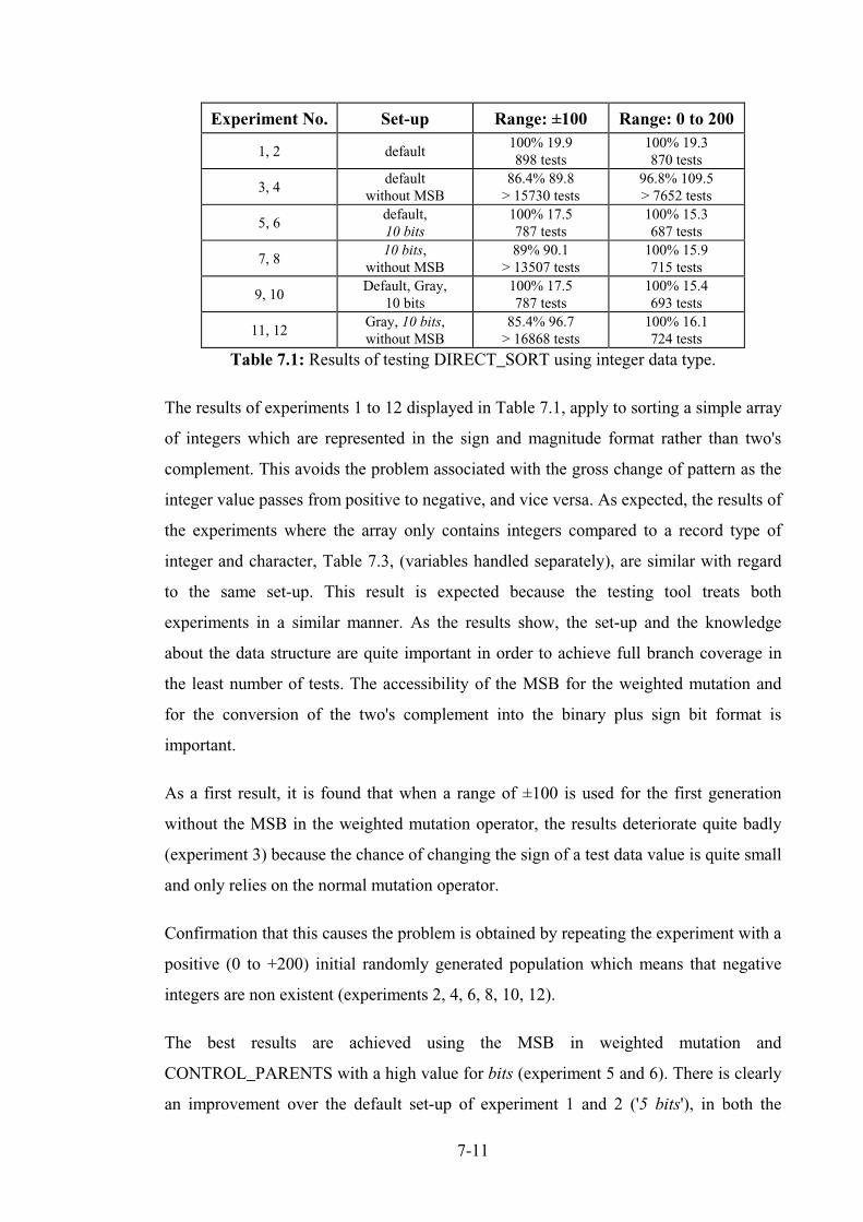
7-11
Table 7.1: Results of testing DIRECT_SORT using integer data type.
The results of experiments 1 to 12 displayed in Table 7.1, apply to sorting a simple array
of integers which are represented in the sign and magnitude format rather than two's
complement. This avoids the problem associated with the gross change of pattern as the
integer value passes from positive to negative, and vice versa. As expected, the results of
the experiments where the array only contains integers compared to a record type of
integer and character, Table 7.3, (variables handled separately), are similar with regard
to the same set-up. This result is expected because the testing tool treats both
experiments in a similar manner. As the results show, the set-up and the knowledge
about the data structure are quite important in order to achieve full branch coverage in
the least number of tests. The accessibility of the MSB for the weighted mutation and
for the conversion of the two's complement into the binary plus sign bit format is
important.
As a first result, it is found that when a range of ±100 is used for the first generation
without the MSB in the weighted mutation operator, the results deteriorate quite badly
(experiment 3) because the chance of changing the sign of a test data value is quite small
and only relies on the normal mutation operator.
Confirmation that this causes the problem is obtained by repeating the experiment with a
positive (0 to +200) initial randomly generated population which means that negative
integers are non existent (experiments 2, 4, 6, 8, 10, 12).
The best results are achieved using the MSB in weighted mutation and
CONTROL_PARENTS with a high value for bits (experiment 5 and 6). There is clearly
an improvement over the default set-up of experiment 1 and 2 ('5 bits'), in both the
Experiment No. Set-up Range: ±100 Range: 0 to 200
1, 2 default100% 19.9898 tests
100% 19.3870 tests
3, 4default
without MSB86.4% 89.8> 15730 tests
96.8% 109.5> 7652 tests
5, 6default,10 bits
100% 17.5787 tests
100% 15.3687 tests
7, 810 bits,
without MSB89% 90.1
> 13507 tests100% 15.9715 tests
9, 10Default, Gray,
10 bits100% 17.5787 tests
100% 15.4693 tests
11, 12Gray, 10 bits,without MSB
85.4% 96.7> 16868 tests
100% 16.1724 tests

7-12
number of tests and in the percentage of the success rate. A distinct improvement is
achieved for the experiments by ensuring that the initial randomly generated population
range is positive e.g. between 0 and 200 (experiment 6). The number of tests are reduced
by 183 compared to experiment 2 ('5 bits') and by 100 compared to experiment 5 (range
±100). In the range from ±100 the improvement is about 111 tests (experiment 5
compared with experiment 1) to get full branch coverage.
The results of the experiments which use the weighted mutation without MSB
(experiments 3, 4 and 7, 8), deteriorate depending on its usage within the experiment. It
can clearly be seen that the experiments in the range of 0 to 200 invariably achieved
better results. Experiment 7 (range ± 100) needed more than 13507 tests, whereas,
experiment 8 (range 0 to 200) need just 715 tests. This shows the importance and
improvement of choosing the right initial range. Experiments with Gray code are
conducted but the results do not improve. They achieve results which are similar to the
default binary code.
Table 7.2: Results using integer data type without CONTROL_PARENTS.
The second set of experiments, Table 7.2, are conducted without the conversion
procedure CONTROL_PARENT, which converts negative values from two's
complement into binary sign and magnitude code. The record is seen as a one bit string
after converting it into a binary format. The bit string is then optimised rather than the
single separate variables of the scalar_type.
Normally one could argue that the results using the two's complement should be worse
than using binary and sign bit because of the different representations (for positive
values binary code and for negative two's complement). In the case of using an initial
range of ±100 the statement is correct. On average about 3 more generations are needed
to achieve full branch coverage using two's complement. The results detoriated rapidly
Experiment No. Set-up Range: ±100 Range: 0 to 200
13, 14Two's complement,
default100% 22.1996 tests
100% 19.7888 tests
15, 16Two's complement,
without MSB68.4% 134.9> 32591 tests
94.4% 173.6> 12415 tests
17, 18Two's complement,
10 bits100% 20.9937 tests
100% 15.4693 tests
19, 20Two's complement,10 bits, without MSB
67.6% 95.2> 32056 tests
100% 15.6710 tests
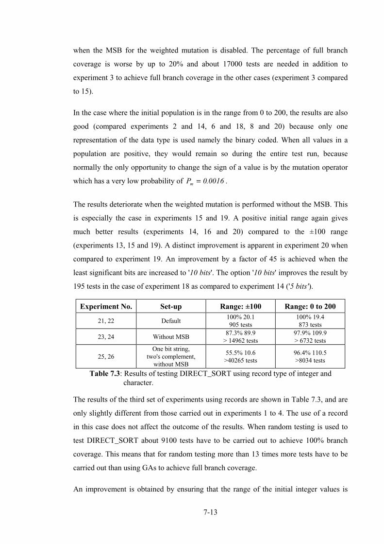
7-13
when the MSB for the weighted mutation is disabled. The percentage of full branch
coverage is worse by up to 20% and about 17000 tests are needed in addition to
experiment 3 to achieve full branch coverage in the other cases (experiment 3 compared
to 15).
In the case where the initial population is in the range from 0 to 200, the results are also
good (compared experiments 2 and 14, 6 and 18, 8 and 20) because only one
representation of the data type is used namely the binary coded. When all values in a
population are positive, they would remain so during the entire test run, because
normally the only opportunity to change the sign of a value is by the mutation operator
which has a very low probability of Pm = 0 0016. .
The results deteriorate when the weighted mutation is performed without the MSB. This
is especially the case in experiments 15 and 19. A positive initial range again gives
much better results (experiments 14, 16 and 20) compared to the ±100 range
(experiments 13, 15 and 19). A distinct improvement is apparent in experiment 20 when
compared to experiment 19. An improvement by a factor of 45 is achieved when the
least significant bits are increased to '10 bits'. The option '10 bits' improves the result by
195 tests in the case of experiment 18 as compared to experiment 14 ('5 bits').
Table 7.3: Results of testing DIRECT_SORT using record type of integer andcharacter.
The results of the third set of experiments using records are shown in Table 7.3, and are
only slightly different from those carried out in experiments 1 to 4. The use of a record
in this case does not affect the outcome of the results. When random testing is used to
test DIRECT_SORT about 9100 tests have to be carried out to achieve 100% branch
coverage. This means that for random testing more than 13 times more tests have to be
carried out than using GAs to achieve full branch coverage.
An improvement is obtained by ensuring that the range of the initial integer values is
Experiment No. Set-up Range: ±100 Range: 0 to 200
21, 22 Default100% 20.1905 tests
100% 19.4873 tests
23, 24 Without MSB87.3% 89.9> 14962 tests
97.9% 109.9> 6732 tests
25, 26One bit string,
two's complement,without MSB
55.5% 10.6>40265 tests
96.4% 110.5>8034 tests
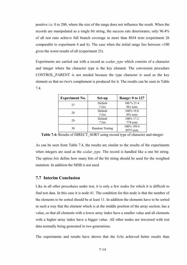
7-14
positive i.e. 0 to 200, where the size of the range does not influence the result. When the
records are manipulated as a single bit string, the success rate deteriorates; only 96.4%
of all test runs achieve full branch coverage in more than 8034 tests (experiment 26
comparable to experiment 4 and 6). The case when the initial range lies between ±100
gives the worst results of all (experiment 25).
Experiments are carried out with a record as scalar_type which consists of a character
and integer where the character type is the key element. The conversion procedure
CONTROL_PARENT is not needed because the type character is used as the key
element so that no two's complement is produced for it. The results can be seen in Table
7.4.
Table 7.4: Results of DIRECT_SORT using record type of character and integer.
As can be seen from Table 7.4, the results are similar to the results of the experiments
when integers are used as the scalar_type. The record is handled like a one bit string.
The option bits define how many bits of the bit string should be used for the weighted
mutation. In addition the MSB is not used.
7.7 Interim Conclusion
Like in all other procedures under test, it is only a few nodes for which it is difficult to
find test data. In this case it is node 41. The condition for this node is that the number of
the elements to be sorted should be at least 11. In addition the elements have to be sorted
in such a way that the element which is at the middle position of the array section, has a
value, so that all elements with a lower array index have a smaller value and all elements
with a higher array index have a bigger value. All other nodes are traversed with test
data normally being generated in two generations.
The experiments and results have shown that the GAs achieved better results than
Experiment No. Set-up Range: 0 to 127
27Default3 bits
100 % 21.4961 tests
28Default5 bits
100% 19.8891 tests
29Default7 bits
100% 17.2774 tests
30 Random Testing100% 199.48975 tests

7-15
random testing. This can be up to 13 times better with respect to the number of tests.
However, when the set-up is not correctly chosen, it could mean that a lot more tests
have to be performed before full branch coverage is achieved (e.g. experiment 25 with
over 40000 tests). This is the case when a record is used as the scalar_type and the
converted bit string is used as one single string for crossover and mutation because of
the representation of the test data which is in the two's complement for negative values
and for positive values in the ordinary binary code with sign and magnitude format. This
happens because the conversion procedure CONTROL_PARENT and the weighted
mutation cannot be used because the record is treated as a one bit string. This means that
the binary and the two's complement coded bit strings are used in crossover which leads
to completely different offspring so that the optimising process is slower and gives
worse results. As soon as only a positive initial range is chosen (0 to 200) for the integer
type (key element) the results improve and in addition by increasing to '10 bits' the
results are similar to experiment 20 where only one integer type forms the scalar_type.
The easiest way would be when the testing tool automatically identifies the structure of
the data type so that it determines where the single bit strings of each variable begin and
end, so that all facilities of the testing tool can be used. This can be achieved by the
attributes 'position, 'first_bit and 'last_bit.
In the next chapter the generated test sets and testing tool are under investigation to
measure the test data adequacy.
8-1
CHAPTER 8
Adequate Test Data
The objective of this chapter is to portray the sets of experiments carried out to measure
the adequacy of the test data generated by the testing tool with respect to error detection.
In the previous chapter branch testing is used in order to satisfy the test criteria. This
strategy proves to be especially difficult when the equality operator is used in the
procedure under test.
The experiments described in this chapter demand that every branch is not only
executed, but also that the test data sets are located close to the subdomain boundary, so
called boundary test data. The advantage of boundary test data is that the test data
should be as close as possible to the predicates (functions or conditions). Most software
errors are at these boundaries, Clarke [1976] and White and Cohen [1980], which are
also called domain errors.
The technique used to measure if the test data is adequate is based on mutation analysis.
Mutation analysis is a fault based testing method which derives test cases (mutants) and
is devised to find particular types of errors. This section describes problems that have
been solved developing the implementation of the technique and the success rate of
producing the boundary test data.
8.1 Adequacy of Test Data
Test adequacy refers to the ability of the test data to ensure that certain errors are not
present in the program under test, i.e. that the program runs successfully on the data set
and all incorrect programs run incorrectly, DeMillo [1987]. However, by showing that
these errors do not occur, does not guarantee the absence of all errors, Weyuker [1983].
The definition of adequacy in relation to test data can be defined as the close proximity
of the data to a subdomain boundary, see chapters 2 and 4. Boundary test data has a
better likelihood of revealing and detecting errors, in contrast to test data which are far
from the boundary, as it was observed by Clarke [1976].
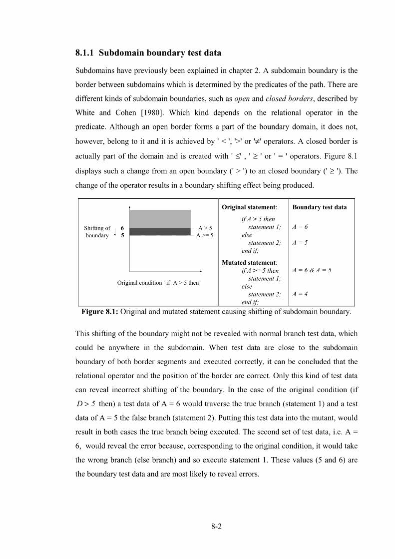
8-2
8.1.1 Subdomain boundary test data
Subdomains have previously been explained in chapter 2. A subdomain boundary is the
border between subdomains which is determined by the predicates of the path. There are
different kinds of subdomain boundaries, such as open and closed borders, described by
White and Cohen [1980]. Which kind depends on the relational operator in the
predicate. Although an open border forms a part of the boundary domain, it does not,
however, belong to it and it is achieved by ' < ', '>' or '≠' operators. A closed border is
actually part of the domain and is created with ' ≤' , ' ≥ ' or ' = ' operators. Figure 8.1
displays such a change from an open boundary (' > ') to an closed boundary (' ≥ '). The
change of the operator results in a boundary shifting effect being produced.
Figure 8.1: Original and mutated statement causing shifting of subdomain boundary.
This shifting of the boundary might not be revealed with normal branch test data, which
could be anywhere in the subdomain. When test data are close to the subdomain
boundary of both border segments and executed correctly, it can be concluded that the
relational operator and the position of the border are correct. Only this kind of test data
can reveal incorrect shifting of the boundary. In the case of the original condition (if
D > 5 then) a test data of A = 6 would traverse the true branch (statement 1) and a test
data of A = 5 the false branch (statement 2). Putting this test data into the mutant, would
result in both cases the true branch being executed. The second set of test data, i.e. A =
6, would reveal the error because, corresponding to the original condition, it would take
the wrong branch (else branch) and so execute statement 1. These values (5 and 6) are
the boundary test data and are most likely to reveal errors.
6 A > 55 A >= 5
Original condition ' if A > 5 then '
Shifting ofboundary
Original statement:
if A > 5 thenstatement 1;
elsestatement 2;
end if;
Mutated statement:if A >= 5 then
statement 1;else
statement 2;end if;
Boundary test data
A = 6
A = 5
A = 6 & A = 5
A = 4

8-3
8.2 Mutation Testing and analysis
In this section a mutation testing strategy is used as a measurement and for evaluation of
the level of adequacy of the test data that can be achieved by the testing tool, using GA
and the random method. It can be said that a test set is adequate if it can distinguish
between the original test program and the set of incorrect mutated programs which are
represented by faults. The goal of mutation testing is to generate test data which reveals
or kills the mutants which simulate typical program errors, Burns [1978].
8.2.1 Overview of mutation analysis
Mutation analysis is a fault-based analysis and is a testing method that measures the
adequacy of a set of independently created test data. Mutation testing tests for specific
and particular types of faults and have been made to the original program by simple
syntactic changes. These mutants reflect common mistakes which are generally
introduced by competent programmers. The set of faults is commonly restricted by two
principles; the competent programmer hypothesis and the coupling effect.
The competent programmer assumption states that competent programmers tend to write
programs that are close to being correct. The restriction of the mutants to single errors is
justified by the principle of the coupling effect which states that simple types of faults
are sensitive enough to detect more complex types of faults. Both assumptions are
experimentally confirmed, Budd et al. [1980] and Offut [1989, 1992].
8.2.2 Detection of mutants
To detect a mutant, it is obvious that the mutated statement must be executed.
Furthermore, the test data has to cause the mutant to produce an incorrect status after
execution of the mutated statement with respect to the original program. Although the
status after execution of the mutated statement is different compared to the original
statement, it is not sufficient to kill the mutant. The status has to propagate through to an
output, to reveal the fault, in order to kill the mutant. If the status of both versions, the
mutated and original program, after the last executed statement is unchanged, then the
mutant is still alive. The essential condition to kill a mutant is, therefore, the request that
the status of the mutated program is incorrect after some execution of the mutated
statement. The status does not have to be specifically incorrect after either the first, or
8-4
last execution, but it should be incorrect after some execution, DeMillo [1993].
Mutation testing can show two things. The percentage of dead mutants reveals how well
the program has been tested. On the other hand, the live mutants reveal either
inadequacies in the used test data set, which reflects on the test data generator (testing
system) or that the original program is incorrect. The presence of live mutants have thus
revealed these faults. If there are live mutants present, then new test data has to be added
until the program tester is satisfied with the proportion of dead mutants.
For example, looking at the quadratic equation solver problem which is correct to the
best of our knowledge, node 1 (see page 5-1) mutated from A = 0 to A = 1, produces for
the test data A = 1, B = 1 and C = 1 the following output 'Error_not_a_quadratic' (node
2). This test data is then put through and compared to the original program where the
output produces: 'Roots_are_real_and_unequal' (node 4) and the mutant is, therefore,
revealed.
In practice it is impossible to reveal and kill all mutants of a program especially when
the changes have no functional effect. These mutants are called equivalent mutants. This
occurs when the outputs of both programs are always the same. These mutants have to
be detected manually and this is one of the most expensive of all current mutation
systems as stated by Offutt [1992]. For example, if the condition in node 6 is mutated
from D = 0 to D ≥ 0 , no difference can ever be found, because only zero and negative
values for D can go this way due to the fact that the condition in node 5 filters out all
positive values for D (D ≤ 0 ). The same output will invariably be produced as in the
original program.
If test data can reveal a high percentage of mutants, it can be said the test data is of high
adequacy (near to the sub domain boundary) and that its likely that the original program
is correct, Budd et al. [1980]. The detection rate, mutation score (MS), of a set of test
data using non-equivalent mutants can be expressed by the definition;
MS TK
M E( ) =
−(8.1)
where M is the number of mutants
E is the number of equivalent mutants
K is the number of mutants which are killed by the test data set T.
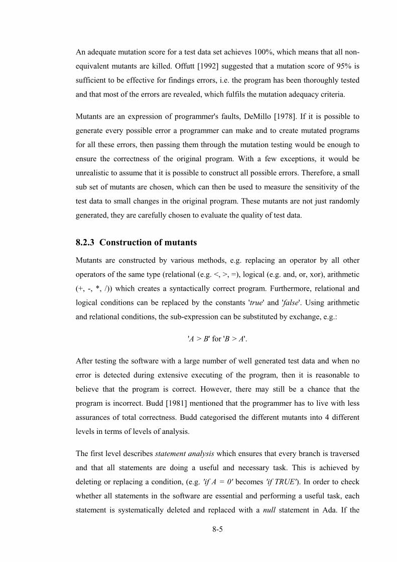
8-5
An adequate mutation score for a test data set achieves 100%, which means that all non-
equivalent mutants are killed. Offutt [1992] suggested that a mutation score of 95% is
sufficient to be effective for findings errors, i.e. the program has been thoroughly tested
and that most of the errors are revealed, which fulfils the mutation adequacy criteria.
Mutants are an expression of programmer's faults, DeMillo [1978]. If it is possible to
generate every possible error a programmer can make and to create mutated programs
for all these errors, then passing them through the mutation testing would be enough to
ensure the correctness of the original program. With a few exceptions, it would be
unrealistic to assume that it is possible to construct all possible errors. Therefore, a small
sub set of mutants are chosen, which can then be used to measure the sensitivity of the
test data to small changes in the original program. These mutants are not just randomly
generated, they are carefully chosen to evaluate the quality of test data.
8.2.3 Construction of mutants
Mutants are constructed by various methods, e.g. replacing an operator by all other
operators of the same type (relational (e.g. <, >, =), logical (e.g. and, or, xor), arithmetic
(+, -, *, /)) which creates a syntactically correct program. Furthermore, relational and
logical conditions can be replaced by the constants 'true' and 'false'. Using arithmetic
and relational conditions, the sub-expression can be substituted by exchange, e.g.:
'A > B' for 'B > A'.
After testing the software with a large number of well generated test data and when no
error is detected during extensive executing of the program, then it is reasonable to
believe that the program is correct. However, there may still be a chance that the
program is incorrect. Budd [1981] mentioned that the programmer has to live with less
assurances of total correctness. Budd categorised the different mutants into 4 different
levels in terms of levels of analysis.
The first level describes statement analysis which ensures that every branch is traversed
and that all statements are doing a useful and necessary task. This is achieved by
deleting or replacing a condition, (e.g. 'if A = 0' becomes 'if TRUE'). In order to check
whether all statements in the software are essential and performing a useful task, each
statement is systematically deleted and replaced with a null statement in Ada. If the
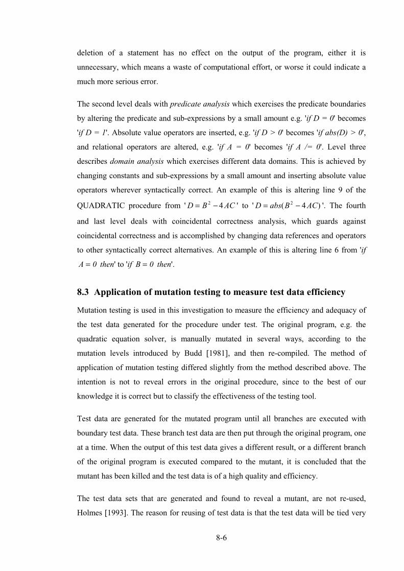
8-6
deletion of a statement has no effect on the output of the program, either it is
unnecessary, which means a waste of computational effort, or worse it could indicate a
much more serious error.
The second level deals with predicate analysis which exercises the predicate boundaries
by altering the predicate and sub-expressions by a small amount e.g. 'if D = 0' becomes
'if D = 1'. Absolute value operators are inserted, e.g. 'if D > 0' becomes 'if abs(D) > 0',
and relational operators are altered, e.g. 'if A = 0' becomes 'if A /= 0'. Level three
describes domain analysis which exercises different data domains. This is achieved by
changing constants and sub-expressions by a small amount and inserting absolute value
operators wherever syntactically correct. An example of this is altering line 9 of the
QUADRATIC procedure from 'D B AC= −2 4 ' to 'D abs B AC= −( )2 4 '. The fourth
and last level deals with coincidental correctness analysis, which guards against
coincidental correctness and is accomplished by changing data references and operators
to other syntactically correct alternatives. An example of this is altering line 6 from 'if
A = 0 then' to 'if B = 0 then'.
8.3 Application of mutation testing to measure test data efficiency
Mutation testing is used in this investigation to measure the efficiency and adequacy of
the test data generated for the procedure under test. The original program, e.g. the
quadratic equation solver, is manually mutated in several ways, according to the
mutation levels introduced by Budd [1981], and then re-compiled. The method of
application of mutation testing differed slightly from the method described above. The
intention is not to reveal errors in the original procedure, since to the best of our
knowledge it is correct but to classify the effectiveness of the testing tool.
Test data are generated for the mutated program until all branches are executed with
boundary test data. These branch test data are then put through the original program, one
at a time. When the output of this test data gives a different result, or a different branch
of the original program is executed compared to the mutant, it is concluded that the
mutant has been killed and the test data is of a high quality and efficiency.
The test data sets that are generated and found to reveal a mutant, are not re-used,
Holmes [1993]. The reason for reusing of test data is that the test data will be tied very

8-7
closely to the boundaries of the predicates and functions in the original procedure. The
non re-use option is chosen in order to make it more difficult for the test data generation
method with each and every mutant. This provides us with the necessary opportunity to
measure the adequacy of the test data generated. Thus, the strengths and weaknesses of
the test data generating method can be explored.
8.3.1.1 Different mutants
The first 14 mutants are of the form of statement analysis which is the first level of
analysis in the proposed mutation testing system of Budd [1981]. They can be seen in
Table 8.1 where the Line No, the Original statement and the Mutated statement are
shown. Eight out of these 14 mutants delete some statements. The other six mutants
replace relational operator with 'true' and 'false'.
Table 8.1: First level of mutation analysis: Statement Analysis.
In the predicate analysis a total number of 24 mutants are created which can be seen in
Table 8.2. Six mutants alter the predicate by a small amount (for the variables A and D).
Three mutants describe the insertion of absolute value operators (abs) into the predicate
sub-expressions. The remaining 15 mutants displaye the alteration of relational
operators.
Mutant No. Line No. Original statement Mutated statement1 7 Quad := Error_not_a_quadratic; null;2 11 Quad := Roots_are_real_and_unequal; null;3 14 Quad := Roots_are_real_and_equal; null;4 16 Quad := Roots_are_complex; null;5 9 D = B2 - 4AC; null;6 6 - 19 if ... end if; null;7 10 - 18 if ... end if; null;8 13 - 17 if ... end if; null;9 6 if A = 0 then if true then10 6 if A = 0 then if false then11 10 if D > 0 then if true then12 10 if D > 0 then if false then13 13 if D = 0 then if true then14 13 if D = 0 then if false then
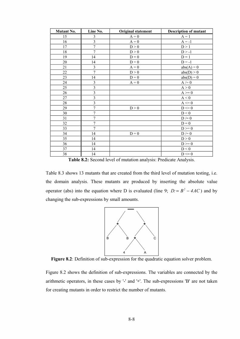
8-8
Table 8.2: Second level of mutation analysis: Predicate Analysis.
Table 8.3 shows 13 mutants that are created from the third level of mutation testing, i.e.
the domain analysis. These mutants are produced by inserting the absolute value
operator (abs) into the equation where D is evaluated (line 9; D B AC:= −2 4 ) and by
changing the sub-expressions by small amounts.
* *
B B * C
4 A
Figure 8.2: Definition of sub-expression for the quadratic equation solver problem.
Figure 8.2 shows the definition of sub-expressions. The variables are connected by the
arithmetic operators, in these cases by '-' and '∗'. The sub-expressions 'B' are not taken
for creating mutants in order to restrict the number of mutants.
Mutant No. Line No. Original statement Description of mutant15 3 A = 0 A = 116 3 A = 0 A = -117 7 D > 0 D > 118 7 D > 0 D > -119 14 D = 0 D = 120 14 D = 0 D = -121 3 A = 0 abs(A) = 022 7 D > 0 abs(D) > 023 14 D = 0 abs(D) = 024 3 A = 0 A /= 025 3 A > 026 3 A >= 027 3 A < 028 3 A <= 029 7 D > 0 D <= 030 7 D < 031 7 D /= 032 7 D = 033 7 D >= 034 14 D = 0 D /= 035 14 D > 036 14 D >= 037 14 D < 038 14 D <= 0
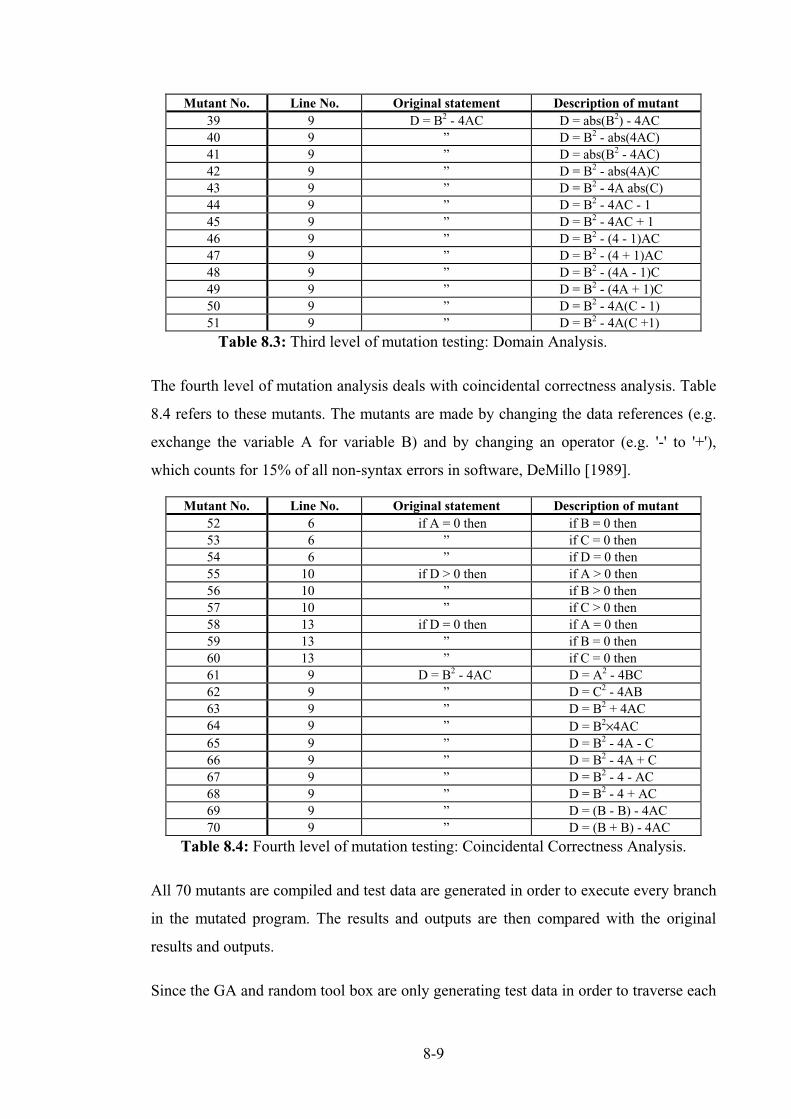
8-9
Table 8.3: Third level of mutation testing: Domain Analysis.
The fourth level of mutation analysis deals with coincidental correctness analysis. Table
8.4 refers to these mutants. The mutants are made by changing the data references (e.g.
exchange the variable A for variable B) and by changing an operator (e.g. '-' to '+'),
which counts for 15% of all non-syntax errors in software, DeMillo [1989].
Table 8.4: Fourth level of mutation testing: Coincidental Correctness Analysis.
All 70 mutants are compiled and test data are generated in order to execute every branch
in the mutated program. The results and outputs are then compared with the original
results and outputs.
Since the GA and random tool box are only generating test data in order to traverse each
Mutant No. Line No. Original statement Description of mutant39 9 D = B2 - 4AC D = abs(B2) - 4AC40 9 ” D = B2 - abs(4AC)41 9 ” D = abs(B2 - 4AC)42 9 ” D = B2 - abs(4A)C43 9 ” D = B2 - 4A abs(C)44 9 ” D = B2 - 4AC - 145 9 ” D = B2 - 4AC + 146 9 ” D = B2 - (4 - 1)AC47 9 ” D = B2 - (4 + 1)AC48 9 ” D = B2 - (4A - 1)C49 9 ” D = B2 - (4A + 1)C50 9 ” D = B2 - 4A(C - 1)51 9 ” D = B2 - 4A(C +1)
Mutant No. Line No. Original statement Description of mutant52 6 if A = 0 then if B = 0 then53 6 ” if C = 0 then54 6 ” if D = 0 then55 10 if D > 0 then if A > 0 then56 10 ” if B > 0 then57 10 ” if C > 0 then58 13 if D = 0 then if A = 0 then59 13 ” if B = 0 then60 13 ” if C = 0 then61 9 D = B2 - 4AC D = A2 - 4BC62 9 ” D = C2 - 4AB63 9 ” D = B2 + 4AC64 9 ” D = B2×4AC65 9 ” D = B2 - 4A - C66 9 ” D = B2 - 4A + C67 9 ” D = B2 - 4 - AC68 9 ” D = B2 - 4 + AC69 9 ” D = (B - B) - 4AC70 9 ” D = (B + B) - 4AC

8-10
branch, they would not be suitable for mutation testing. There may be many test data in
a subdomain which could prove to be satisfactory in traversing branches, but only a
limited amount of boundary test data can reveal shifting of boundaries. For this reason
the program testing tool is expanded, and altered in the sense that boundary test data
have to be generated. The advantage of using boundary test data is that there is a higher
chance of revealing errors, the disadvantage being that the search procedure for
boundary test data may be longer.
Boundary test data generation is achieved by looking at one node until the predicate of
the node is traversed as closely as possible. This means that the node is not set to be
traversed with any possible test data set from the sub domain. It is only set to be
traversed when the boundary test data of a predicate is generated or a certain number of
attempts (generations) are completed. For each node the fittest test data is stored in the
database.
The criterion for this new method is that the branch is only set to be traversed when the
highest possible fitness (boundary test data) is achieved, where the fitness values are
directly evaluated by the predicate conditions. To traverse a node with boundary test
data, a certain number of generations (tests) can be pre-defined (similar to a threshold)
for the node. The pre-defined generations can be used just for observing this node in
order to get closer to the boundary of the predicate. If no boundary test data are
produced, after using the certain number of pre-defined generations (this can vary from
node to node), the test data with the highest fitness will be taken instead which is
automatically stored in the data base.
The counting of the pre-defined generations only starts when the testing tool is actually
searching and trying to traverse that particular node. If the test data traverses a node
which is not under investigation, then the test data is stored if it has a higher fitness than
the data already in the database.
8.3.1.2 First mutation results
In the initial experiment of mutation testing, boundary test data are generated in order to
traverse all branches of the mutated procedure under test. After test data are generated
for all the branches and stored, they are put through the original procedure. Any

8-11
difference in the expected and actual output from the mutant kills that mutant.
The first test runs show that no test data are generated for node 7 (D < 0) with D = −1 .
Since no integer combination of A, B and C exist to give a value of D = −1 or D = −2
the boundary test data is D = −3 ; the testing tool always exceeds the pre-defined
number of generations for node 7 and abandoned the run for this node because the
system does not look for a D = −3 . A new stopping condition is introduced in order to
avoid many unnecessary tests. This is due to the fact that the boundary test data of
D = −3 could have been already generated without realisation, thereby resulting in the
testing tool still performing a search for the value of D = −1 . This new condition stops
the specific search of a test data for a certain node if the fitness reaches a certain
threshold. Therefore, after a certain number of generations, it is assumed that the test
data are close enough to the boundary of the subdomain. This means a decrease in the
number of generations and a better comparison between the use of random and GA
methods of generating of test data.
Two strategies are adopted using mutation testing. In order to perform mutation analysis
two procedures of the same kind are used; the original procedure and the mutated
procedure. Test data are always generated for the procedure under test. In one case, the
data are produced for the mutated procedure and then in the next experiment for the
original procedure. The answer to the question here is to find out how robust are GAs to
reveal the mutants, in other words can GAs generate adequate test data (hypothesis 4)
and for which, the original or the mutant, the test data should be generated for. As it can
be seen later generating test data for the original program is better than for the mutant.
From all 70 mutants, 6 mutants could not be revealed at all and 14 mutants are only
partly revealed (success rate between 42% and 99%) when test data are generated for the
mutant. On taking a closer look at the six unrevealed mutants, the result is that four of
them (mutants 21, 23, 36 and 39) are equivalent mutants which means that they always
produced the same output as the original procedure. That means they could not be
distinguished by their functionality. Thus only two mutants are not revealed at all
(mutants 26 and 28).
Therefore, the mutation score is MS = 0 97. (97%) when including the partly revealed
mutants. This is in excess of Offutt's stated sufficient mutation score threshold of 95%.

8-12
The reason why the two mutants could not be revealed is because the predicate for node
2 is changed from A = 0 to A ≥ 0 (mutant 26) and A ≤ 0 (mutant 28). Since boundary
test data are generated, the testing tool would generate the value A = 0 for node 2 in the
mutant and the original program. The only difference at this point is that only negative
values are used for the rest of the program to traverse the remaining nodes. The
boundary does not shift. This kind of error could not be revealed with the current
method.
However, generating test data for the original procedure, only mutant 40 could not be
exposed besides the four equivalent mutants and 13 mutants are only partly revealed
with variations of 33% to 97% success of the test runs.
8.3.1.3 Improving the testing tool with regard to mutation testing
In order to achieve a better mutation score (which means to kill the unrevealed and
partly unrevealed mutants ) more boundary test data have to be generated. Where '='
(equal) or '/=' (unequal) operators are used, two sets of boundary test will be generated
on both sides of the subdomain boundary, see chapter 4. For all other predicates only
one boundary test has to be produced. That means, for node 3, two boundary test data
has to be generated and stored for each side of the border in order to traverse this node
successfully. In addition the strategy of the mutation testing is changed in the sense that
every test data which is put through the procedure under test and produced an output,
has to be entered straight away into the original procedure in order to compare the
output. If any difference in the output is noticed, the mutant would be instantly killed
and the test run stops in order to start the next test run. This should give information of
how many generations are actually needed in order to reveal the mutants and to compare
the results with a random testing.
Four different sets of mutation testing experiments have been conducted. In the first set
of experiments test data are generated for the mutated procedure. Therefore, the fitness
functions are adapted for the mutant. The second column of the results tables (GA
mutant in test procedure, e.g. Table 8.5) refers to the results of this experiment. The
second experiment (third column: Random mutant in test procedure) uses a random
number generator in order to generate the test data. Columns four (using GA), and five
(using random), display the results of a different approach. This time, boundary test data
8-13
sets are generated for the original procedure, and then these are put into the mutant. This
should show whether boundary test data are important, what kind of influences these
have regarding the software, and for which procedure, mutant or original, it is better to
adapt the generation of test data. The results are displayed as the percentage of
successful test runs and number of required tests.
8.3.1.4 Test results
Using this new method, all non-equivalent mutants are revealed in less than or about
1344 tests using both GA approaches, which corresponds to a mutation score of 100%.
Each mutant runs 1000 times in order to get a good statistical result of how many
generations are needed. Table 8.5 displays the results for the statement analysis, Table
8.6 refers to predicate analysis, Table 8.7 shows the results of domain analysis and Table
8.8 shows the results of the coincidental correctness analysis. Displayed in the tables
below are the percentage of revealed mutants in test runs and the required number of
tests.
In the first set of experiments in the statement analysis all mutants are revealed by using
GAs. Only two of the mutants (3 and 14) required about 1340 tests. The other non-
equivalent mutants are revealed in the first or second generation. These mutants are also
easily revealed by random testing, where boundary test data are not necessarily needed.
However, random testing achieves much worse results for mutants 3 and 14 (about 7060
tests) which is shown in Table 8.5.

8-14
Table 8.5: Results of statement analysis.
For each of these two mutants, the mutant can only be revealed by generating a test data
which will result in D = 0 and traverse node 6, that explains the high number of
required tests. Table 8.6 shows the results of predicate analysis.
Table 8.6: Results of predicate analysis.
Mutant No. GA mutant intest procedure
Random mutantin test procedure
GA mutant inoriginal proc.
Random mutantin original proc.
1 100% in 144 100% in 202 100% in 142 100% in 1942 100% in 3 100% in 3 100% in 3 100% in 33 100% in 1320 99.4% in 7536 100% in 1373 99.6% in 68744 100% in 4 100% in 4 100% in 4 100% in 45 100% in 3 100% in 3 100% in 3 100% in 36 100% in 10 100% in 10 100% in 3 100% in 37 100% in 3 100% in 3 100% in 3 100% in 38 100% in 4 100% in 4 100% in 4 100% in 49 100% in 3 100% in 3 100% in 3 100% in 310 100% in 138 100% in 203 100% in 140 100% in 20411 100% in 4 100% in 4 100% in 4 100% in 412 100% in 3 100% in 3 100% in 3 100% in 313 100% in 4 100% in 4 100% in 4 100% in 414 100% in 1309 99.7% in 7076 100% in 1297 99.0% in 7152
Mutant No. GA mutant intest procedure
Random mutantin test procedure
GA mutant inoriginal proc.
Random mutantin original proc.
15 100% in 88 100% in 99 100% 95 100% 10216 100% in 90 100% in 102 100% 96 100% 9917 100% in 1133 99.1% in 4445 100% 1066 97.9% 410918 100% in 1354 99.2% in 7412 100% 1335 99.2% 688419 100% in 1334 99.8% in 7152 100% 1373 99.5 689320 100% in 1311 99.0% in 6989 100% 1364 99.3% 678821 0% in 4407
not detectable0% in 19508
not detectable0% 4445not detectable
0% 19652not detectable
22 100% in 4 100% in 4 100% 4 100% 423 0% in 4503
not detectable0% in 19392
not detectable0% 4359not detectable
0% 19690not detectable
24 100% in 3 100% in 3 100% in 3 100% in 425 100% in 3 100% in 4 100% in 3 100% in 426 100% in 4 100% in 4 100% in 4 100% in 327 100% in 4 100% in 4 100% in 3 100% in 328 100% in 4 100% in 4 100% in 3 100% in 429 100% in 3 100% in 3 100% in 3 100% in 330 100% in 3 100% in 3 100% in 3 100% in 331 100% in 4 100% in 4 100% in 4 100% in 432 100% in 3 100% in 3 100% in 3 100% in 333 100% in 1364 99.2% in 7103 100% in 1392 99.7% in 680734 100% in 4 100% in 4 100% in 4 100% in 435 100% in 1277 99.3% in 7162 100% in 1325 99.6% in 738336 0% in 4359
not detectable0% in 18759
not detectable0% in 4368not detectable
0% in 19671not detectable
37 100% in 4 100% in 4 100% in 4 100% in 438 100% in 4 100% in 4 100% in 4 100% in 4
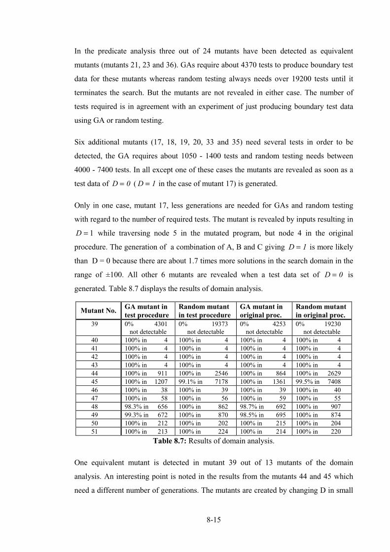
8-15
In the predicate analysis three out of 24 mutants have been detected as equivalent
mutants (mutants 21, 23 and 36). GAs require about 4370 tests to produce boundary test
data for these mutants whereas random testing always needs over 19200 tests until it
terminates the search. But the mutants are not revealed in either case. The number of
tests required is in agreement with an experiment of just producing boundary test data
using GA or random testing.
Six additional mutants (17, 18, 19, 20, 33 and 35) need several tests in order to be
detected, the GA requires about 1050 - 1400 tests and random testing needs between
4000 - 7400 tests. In all except one of these cases the mutants are revealed as soon as a
test data of D = 0 (D = 1 in the case of mutant 17) is generated.
Only in one case, mutant 17, less generations are needed for GAs and random testing
with regard to the number of required tests. The mutant is revealed by inputs resulting in
D = 1 while traversing node 5 in the mutated program, but node 4 in the original
procedure. The generation of a combination of A, B and C giving D = 1 is more likely
than D = 0 because there are about 1.7 times more solutions in the search domain in the
range of ±100. All other 6 mutants are revealed when a test data set of D = 0 is
generated. Table 8.7 displays the results of domain analysis.
Table 8.7: Results of domain analysis.
One equivalent mutant is detected in mutant 39 out of 13 mutants of the domain
analysis. An interesting point is noted in the results from the mutants 44 and 45 which
need a different number of generations. The mutants are created by changing D in small
Mutant No. GA mutant intest procedure
Random mutantin test procedure
GA mutant inoriginal proc.
Random mutantin original proc.
39 0% 4301not detectable
0% 19373not detectable
0% 4253not detectable
0% 19230not detectable
40 100% in 4 100% in 4 100% in 4 100% in 441 100% in 4 100% in 4 100% in 4 100% in 442 100% in 4 100% in 4 100% in 4 100% in 443 100% in 4 100% in 4 100% in 4 100% in 444 100% in 911 100% in 2546 100% in 864 100% in 262945 100% in 1207 99.1% in 7178 100% in 1361 99.5% in 740846 100% in 38 100% in 39 100% in 39 100% in 4047 100% in 58 100% in 56 100% in 59 100% in 5548 98.3% in 656 100% in 862 98.7% in 692 100% in 90749 99.3% in 672 100% in 870 98.5% in 695 100% in 87450 100% in 212 100% in 202 100% in 215 100% in 20451 100% in 213 100% in 224 100% in 214 100% in 220
8-16
amounts i.e. by adding and subtracting the value 1 from D. By changing the function D,
the subdomains for the different paths changes as well. That means that for traversing
node 4 the new subdomain is B AC2 4 1− > − and for node 6, B AC2 4 1− = − in mutant
45. The latter corresponds to an infeasible path because there is no combination that
could match D = −1 . The only test data which could reveal this mutant is a test data of
D = 0 which causes node 4 to be traversed in the mutant, and node 6 in the original
procedure. However, it appeared that mutant 44 can be killed with two different
solutions, which result in fewer required generations. For node 4 the actual condition in
the mutant is B AC2 4 1− > (D > 1) and for node 6, B AC2 4 1− = (D = 1 ) which
would result in different nodes being traversed in both cases compared to the original
procedure. Both paths are feasible, therefore, the probability of generating one of these
solutions in order to reveal the error is higher than in mutant 45.
Mutants 48 and 49, which are created by changing the sub-expression '4A' by a small
amount (-1 and +1), cannot always be revealed in all test runs. The reason for this event
is that if the variable C = 0 the mutant cannot be killed. This leads to a zero solution
( B C= = 0 ).
In the last set of mutation results, the coincidental correctness analysis, in Table 8.8,
only three results are interesting enough to mention in more detail. These are the results
of mutants 58, 59 and 61. These mutants originated by exchanging variable names with
existing ones, (i.e. D = 0 into A = 0 , B = 0 and C = 0 ).
By creating mutant 58, an infeasible path is produced in node 6. The condition in node 6
of 'if A = 0 ' cannot become true because zero values for A are not allowed after node 2
since they have already been filtered out. Only a test data of D = 0 which traverses the
mutant node 7 is able to reveal the error, by traversing node 6 in the original procedure.
This is reflected in the number of required tests (1340 tests).
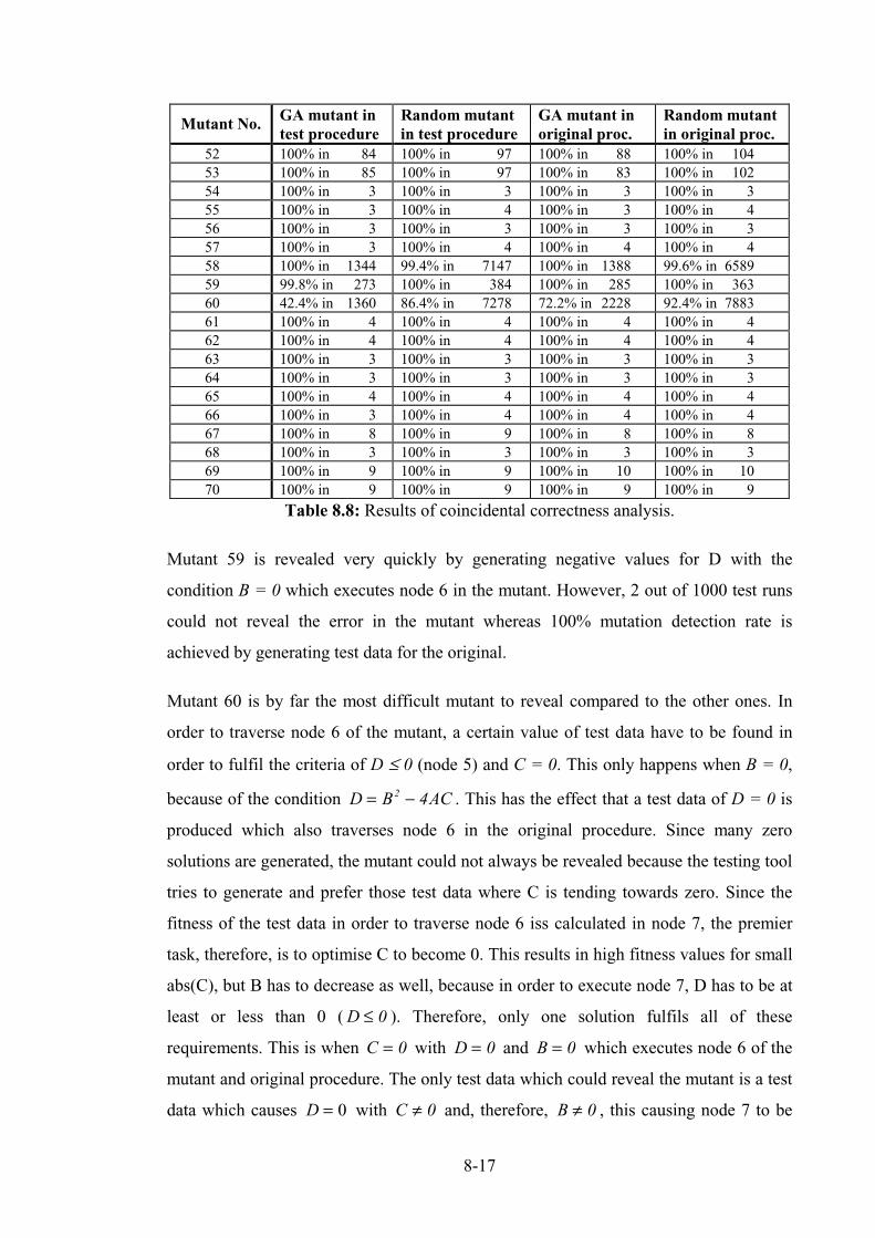
8-17
Table 8.8: Results of coincidental correctness analysis.
Mutant 59 is revealed very quickly by generating negative values for D with the
condition B = 0 which executes node 6 in the mutant. However, 2 out of 1000 test runs
could not reveal the error in the mutant whereas 100% mutation detection rate is
achieved by generating test data for the original.
Mutant 60 is by far the most difficult mutant to reveal compared to the other ones. In
order to traverse node 6 of the mutant, a certain value of test data have to be found in
order to fulfil the criteria of D ≤ 0 (node 5) and C = 0. This only happens when B = 0,
because of the condition D B AC= −2 4 . This has the effect that a test data of D = 0 is
produced which also traverses node 6 in the original procedure. Since many zero
solutions are generated, the mutant could not always be revealed because the testing tool
tries to generate and prefer those test data where C is tending towards zero. Since the
fitness of the test data in order to traverse node 6 iss calculated in node 7, the premier
task, therefore, is to optimise C to become 0. This results in high fitness values for small
abs(C), but B has to decrease as well, because in order to execute node 7, D has to be at
least or less than 0 (D ≤ 0 ). Therefore, only one solution fulfils all of these
requirements. This is when C = 0 with D = 0 and B = 0 which executes node 6 of the
mutant and original procedure. The only test data which could reveal the mutant is a test
data which causes D = 0 with C ≠ 0 and, therefore, B ≠ 0 , this causing node 7 to be
Mutant No. GA mutant intest procedure
Random mutantin test procedure
GA mutant inoriginal proc.
Random mutantin original proc.
52 100% in 84 100% in 97 100% in 88 100% in 10453 100% in 85 100% in 97 100% in 83 100% in 10254 100% in 3 100% in 3 100% in 3 100% in 355 100% in 3 100% in 4 100% in 3 100% in 456 100% in 3 100% in 3 100% in 3 100% in 357 100% in 3 100% in 4 100% in 4 100% in 458 100% in 1344 99.4% in 7147 100% in 1388 99.6% in 658959 99.8% in 273 100% in 384 100% in 285 100% in 36360 42.4% in 1360 86.4% in 7278 72.2% in 2228 92.4% in 788361 100% in 4 100% in 4 100% in 4 100% in 462 100% in 4 100% in 4 100% in 4 100% in 463 100% in 3 100% in 3 100% in 3 100% in 364 100% in 3 100% in 3 100% in 3 100% in 365 100% in 4 100% in 4 100% in 4 100% in 466 100% in 3 100% in 4 100% in 4 100% in 467 100% in 8 100% in 9 100% in 8 100% in 868 100% in 3 100% in 3 100% in 3 100% in 369 100% in 9 100% in 9 100% in 10 100% in 1070 100% in 9 100% in 9 100% in 9 100% in 9
8-18
traversed in the mutant and node 6 in the original. Mutant 60 is revealed in only 42.4%
in all test runs. The mutant detection rate improves when the test data are generated for
the original procedure (72.2%) because the target is then to generate any test data which
cause D = 0 and not in addition C = 0 . The results for the random testing method also
improved by about 11% when test data is generated for the correct procedure and not for
the mutant. Moreover, in both cases random testing have a higher detection rate, but it
has to be paid for in the higher number of tests required. This is due to the fact that
random testing has a better chance of producing a non zero solution since many more
test data are generated until all branches are tested with boundary test data.
8.4 Interim conclusion
The results for the first set of experiments, where only the final boundary test data are
used to put through the original procedure, turns out to be different depending on which
procedure (mutant or original) the test data are generated for. In the first case two and 14
non-equivalent mutants have only partly been revealed (success under 100%), whereas,
using the original as the procedure under test, one non-equivalent mutant is not revealed
and 13 mutants are not always revealed. Thus, these results show that adaptive boundary
test data generation for the original procedure is slightly better than for the mutant.
In the improved version of mutation testing every single test data is put through both
procedures (mutant and original) and two boundary data have to be produced depending
on the relational operator per node, resulting in all mutants being revealed except for
four. These four mutants 48, 49, 59 and 60 are only partly revealed when the test data
are generated for the mutated procedure. Only three mutants, mutant 48, 49 and 60, are
only partly revealed when generating test data for the original procedure. The GA
always requires fewer tests than random testing in order to complete the task of
generating boundary test data and revealing the mutants.
All partly revealed mutants are revealed in at least 98% of all test runs except mutant 60.
Including the partly revealed mutants a mutation score of 100% has been achieved,
leaving aside mutant 60, a mutation score of about 99% is achieved. 62 out of 66 non-
equivalent mutants are always killed in every test run which means strictly a mutation
score of 94% for generating test data for the mutant and 63 out of 66 (96%) for the
original procedure being the procedure under test. This indicates again that generating
8-19
test data for the original program is slightly better than for the mutant. This and the fact
that GAs can generate adequate test data, confirms hypothesis 4.
When observing the results of these experiments, it can be seen that there is not much
difference in these for the GA experiments (see columns 2 and 4). The same situation
applies for random testing (see columns 3 and 5). For each procedure under test the
boundary test data are generated separately (either for the mutant or original) and GAs
have a better mutation detection rate in all cases except one, mutant 60. For this single
mutant random testing proves to be better.
A way of increasing the detection rate is to compare in the mutant and the original other
kinds of computational effects, e.g. intermediate calculations, which means monitoring
statement executions during program testing. In this case, it means trying to monitor D
for each calculation. This kind of analysis will lead to weak mutation analysis, derived
by Foster [1980] and is related to ideas on circuit testing where the most widely studied
physical faults of digital circuits errors are 'stuck at' line faults. In the single fault model
for circuits, test data are derived to reveal the presence or absence of gates which are
stuck at 0 or 1.
Some of the mutant's effect is that they produce an overflow error because the integer
value calculation of D is greater than the highest possible (232). This is due to the change
of the function of D in some mutants, e.g. mutant 64 (D B AC= ×2 4 ). Thus the
overflow error occurrs just in the mutant and not in the original in this case. It can also
be the other way round, e.g. mutant 69 (D B B AC= − −( ) 4 ). The best example is
mutant 5, where the calculation of D is replaced by a null statement, so that a calculation
could not cause an overflow error in the mutant at all.
The results have shown that the attempt to generate test data automatically to satisfy the
mutation adequacy criteria by revealing mutants can be achieved by using GA in most
cases. They also show that the testing tool (GA) is suitable in producing boundary test
data where it is necessary, in order to kill the mutants, whereas random testing needs
many tests.
The most time consuming problem in these experiments is the generation of all these
mutants since they are created and compiled manually. Howden [1982] mentioned that a

8-20
software of m lines has an estimated m2 mutants. This would imply about 400 mutants
for the quadratic procedure. This would consume too much time for creating the
mutants. Therefore, only a carefully selected number of mutants are tested.
In the next and last chapter the experiments and the testing tool are reviewed and
conclusions are drawn from them.
9-1
CHAPTER 9
Review and Conclusion
In this chapter the thesis is summarised and conclusions are drawn from the results and
analysis of the experiments.
9.1 Review of the project
The idea and objective of this research project was to investigate the effectiveness of test
data generation using Genetic Algorithms. Therefore, a test harness was developed in
order to apply branch, boundary and loop testing criteria which was to iterate a loop
zero, one, two, and more than two times. Several experiments and test runs were carried
out to measure the effectiveness of using GAs for generating test data and to verify
hypotheses which have been listed in section 1_2. The effectiveness of the GA results
were compared to the effectiveness of random testing with regard to the required number
of tests and amount of CPU time used.
9.2 Summary
From the work reported in this thesis and from the results of the analysis of all
experiments, a number of conclusions can be drawn. Hypothesis 2 was confirmed that
there are standard sets of parameter settings for different features of the program under
test. We have seen that the difficulty in choosing a good internal representation for the
search space increases with its complexity. Similar care has to be taken to provide an
effective feedback mechanism, called the fitness function. These and more issues are
discussed in the following sections.
9.2.1 Operators
The idea of the various crossover operators is to try to achieve the recombination of
above average genetic material from parents of above average fitness. All crossover
operators share the same idea whereas they have considerably different mechanics.
Experiments have shown that uniform crossover gave the best performance with regard
to the number of required tests and the success rate. Uniform crossover required up to

9-2
24% fewer tests for the QUADRATIC procedure, 32% fewer tests using the
TRIANGLE classifier procedure and about 40% fewer tests for the REMAINDER
procedure (confirming hypothesis 2_3). In general, the crossover operator was important
for the optimisation process and combining good building blocks of parents.
Experiments without the crossover operator showed for the QUADRATIC procedure a
decrease in the GA's performance by requiring about 56% more tests which means that
the building blocks are combining at a slower rate.
The mutation operators have a very important role. With a reduced or zero mutation rate
the performance of test data generation decreased severely. For example for the
QUADRATIC procedure, when the default Pm was reduced by a factor of 5, only 63%
of all tests were successful in achieving full branch coverage instead of 100% with the
default PSm = 1(confirming hypothesis 2_5). Disruption of the chromosomes plays an
important role for the GA with the intention of creating better building blocks. In the
right quantity, disruption prevents premature convergence and loss of genetic material
and thus preventing being stuck at a local optimum. The weighted mutation operator
which was involved when the population seemed to be stuck at a local optimum, plays a
significant part in the optimisation process. In theory, as long as the mutation is active, it
is guaranteed that every point in the space has a non-zero probability of being generated.
The selection and survival operators have shown how important they are. The survival
of offspring into the next generation was always based upon their fitness value, whereas
the selection for the crossover and mutation was performed either by corresponding to
their fitness or randomly. This was dependent on the kind of search space (hypothesis
2_2). If there was only one global optimum to search for, the fitness based selection was
superior, as for the linear and binary search, whereas the random selection performed
better when many global optima were in the search space, e.g. for the quadratic and
triangle classifier procedures.
9.2.2 Data types, fitness function and program structures
Several different data types were used for the various procedures under test such as
integer, float and character variables and also in combinations with records and arrays.
These different data types had no influence on the performance of the GA as long as the

9-3
testing tool knew what kind of data structure and variables were used in order to utilise
all its facilities. Two main fitness functions were used. The first is a simple numeric
method which is based on a reciprocal function and which may be used only for simple
data structures. Secondly a more general approach used a Hamming fitness function,
weighted and unweighted, which had no problems in handling these data structures and
types. Overall the Hamming fitness function turned out to be the most consistent and
reliable fitness function in describing the fitness of the test data, whereas, the reciprocal
fitness function favours too strongly smaller values of the test data.
Xanthakis et al. [1992] and Watkins [1995] have recently applied GAs to the testing
problem and using different approaches of applying fitness function. Watkins uses
fitness functions based on the number of times a particular path is executed. This means
that the more often the same path is taken the lower will be the fitness value. In
comparison with Watkin's system using the triangle classifier procedure our testing
system achieved full coverage in less than a fifth of the number of tests. This can be
explained by the nature of Watkins fitness functions which can irritate the system
because a test set can be of very low fitness while it is very close to execute an
untraversed branch. M. Roper from the University of Strathclyde (by private
communication) uses as a fitness for an individual the coverage it achieves of the
software under test. Unfortunately, no results are yet published or what kind of software
under test have been used.
Different program structures such as 'if' and 'loop' conditions have been tested. In
chapter 6 special emphasise was put onto generating test data for different number of
iterations that a loop will perform (zero, once, twice and more than twice). GAs had no
problems in doing this, so confirming hypothesis 3.
9.2.3 Representation; Gray vs. binary
The easiest form of representation was the binary format which was then converted into
a sign and magnitude representation where the MSB was the sign bit. The binary
representation achieved better results in connection with the Hamming fitness function.
Whereas Gray coded chromosomes with the numerical reciprocal fitness function
required fewer tests than binary format in accordance with hypothesis 2_1. Using Gray
code and Hamming fitness could mean that the GA is too disruptive. Changing the LSB
9-4
of a Gray coded represented chromosome would not result in changing the data type by
one unit. It could be a very large change. Those changes of the LSBs are made by using
the weighted mutation. Using Hamming fitness to calculate the fitness, resulted in a total
breakdown of the performance measurement.
9.2.4 Adequacy criteria and mutation testing
In chapter 8 the adequacy of the test data generated by the testing tools was under
investigation. A set of test data is considered adequate if a program behaves correctly on
the test data but on incorrect programs behave incorrectly.
It was shown that the GA produced test data to distinguish the mutant from the original,
and a mutation score of 100% was achieved, including partly revealed mutants. GAs are
highly effective at generating boundary value tests, which was confirmed by mutation
testing which confirms hypothesis 4.
9.2.5 Random testing vs. GA testing
The results of random testing and GA testing have been compared. GAs always required
fewer tests than random testing and needed less CPU time when the density of the
solutions were quite small. GA testing needed up to two orders of magnitude fewer tests
than randomly generated test sets. It was shown that using GAs was more efficient than
random testing and more effective in the generating test data, which justifies hypothesis
1. Random testing had major problems with generating test data where the equality
operator was used (small solution sub-domains). The recorded CPU time per test data set
is also a good indicator of the complexity of the software under test.
A further disadvantage of random testing over using GA is the fact, that if the random
generated input test data range is producing test sets which are located in a wrong area,
e.g. for the triangle in the range from -100 to 0, not all branches of the software are able
to be traversed. Whereas using GAs there is always the probability on generating the
required test sets. The only disadvantage being that GA required more CPU time per test
data generation.
9-5
9.3 Conclusion
The overall aim was to develop a self-learning algorithm that has the ability to process
and incorporate new information as the work environment changes (changing from one
predicate to the next). The GAs give good results and their power lies in the good
adaptation to the various and fast changing environments.
The primary objective of this project was to propose a GA-based software test data
generator and to demonstrate its feasibility. The experimental results show that this was
achieved. The main advantage of the developed testing tool is the strength of GAs, in
that the relationship between the predicate under investigation and the input variables
may be complex and need not be known. Instrumentations capture the actual values of
the predicates, so that the fitness can be based on these values.
Although some of the procedures under test are small, they contain complex non linear
branch conditions with complex data types which use nested 'if' and 'loop' conditions. It
is these non linear problems where the GAs develop their strengths.
The quadratic procedure (chapter 5) was used to establish the feasibility of using GAs to
generate test sets and to determine the most appropriate parameters for the GAs. The
GAs were then applied to various larger and more complex procedures with different
characteristics. All tests clearly show that the GA generated test data are significantly
better than randomly generated data.
An automated oracle, which can determine whether or not a program has been correctly
executed on a given test case, is required to evaluate large numbers of automatically
generated test data sets. An oracle is important because branch coverage does not imply
that the executed branches are correct, Müllerburg [1995]. Such an oracle can be
realised by post condition or formal specification. This can be achieved by for example
post conditions. If post conditions are not available, a subset of test sets were chosen,
which had the highest fitness value (close to the boundary) of each branch to reduce the
number of test data to check.
The results using GAs can be improved by more research into the performance of the
various operators and testing harness strategy in order to guide the test data generation
process to the required branches and nodes to traverse. However, the results of using

9-6
random testing cannot be changed, since the test data generation process does not
depend on heuristics or algorithms. An advantage of this approach is that the test harness
can easily be changed depending on the testing criteria without influencing the GAs.
The previous problems regarding software testing, mentioned in chapter 2, contrast with
our GA testing tool which does not require any analysis or interpretation of the code so
that in addition the form of the predicate need not be known, thus avoiding the problems
with e.g. symbolic execution. Functions or procedures calls and dynamic data types are
no problems for our system. The GA testing tool gets the predicate function value by
suitable code instrumentation. These instrumentation statements keep a record of
branches and statements that are executed during the testing of a program which do not
affect the functional behaviour. Each time the program under test performs a significant
event, the occurrence of that event is recorded in order to measure test coverage, Ince
[1989].
GAs show good results in searching the input domain for the required test sets, however,
other methods like simulated annealing or tabu search may be an effective testing tool,
too. GAs may not be the answer to the approach of software testing, but do provide an
effective strategy.
9.4 Contribution to published Literature
During the period of the research, details and results of this investigation have been
reported and published in various conferences and journals. These are as follows:
I. Sthamer, H. - H., Jones, B. F. and Eyres, D. E., Generating test data for ADA
generic procedures using Genetic Algorithms, Proceedings of ACEDC '94, PEDC,
University of Plymouth, UK., pp. 134-140, 1995;
II. Jones, B. F., Sthamer, H. - H., Yang, X. and Eyres, D. E., The automatic generation
of software test data using adaptive search techniques, Proceedings of third Int.
Conf. on Software Quality Management SQM '95, Seville, pp. 435 - 444, 1995;
III. Jones, B. F., Sthamer, H. - H. and Eyres, D. E., Generating test data for ADA
procedures using Genetic Algorithms, GALESIA '95, IEE / IEEE International
Conference on: Genetic Algorithms in Engineering Systems: Innovations and
Applications; Sheffield University, September 1995, 65 - 70, 1995;

9-7
IV. Jones, B. F., Sthamer, H. H. and Eyres, D. E., Genetic Algorithms : a new way of
evolving test sets, Eurostar '95, 27 - 30 November, Olympia Conference Centre,
London, UK, 24/1 - 24/10, 1995;
V. Jones, B. F., Sthamer, H. H. and Eyres, D. E., Use of genetic algorithms to generate
test data automatically, Software Engineering Journal, accepted;
VI. Jones, B. F., Sthamer, H. H. and Eyres, D. E., An empirical investigation into the
use of Genetic Algorithms to generate test data automatically, IEEE Transaction on
Software on Software Engineering, accepted for publication.
9.5 Further studies
One major aspect of future work is to develop new operators which make the search and
optimisation process easier and faster. New crossover and mutation operators are under
investigation. Operators such as crossover, mutation, selection and survive procedures
have to evolve or adapt their probability with the search space (fixed parameters should
be avoided). This would improve and automate the parameter settings for the GAs which
makes it easier to run.
Although the instrumentation of the procedures under test is straight forward and
corresponds to fixed rules, an automated tool to insert those procedure calls would
considerably simplify the entire process.
A new approach to using GA is using them in parallel such as it is in nature, Hesser and
Männer [1990], Cohoon et al. [1987] and Prettey et al. [1987] who mentioned that they
have a distinctive advantage because for example the population is split into several
smaller sub populations. Depending on the method these sub populations can then
exchange genetic material or entire chromosomes to form a new population. The parallel
GAs are distinguished by their faster searching because now these sub populations can
explore the search space more thoroughly.
Data flow analysis may be used to identify those variables which are involved in the
search process, so that only those will be used in order to cut down the CPU time as is
the case in the triangle classifier and the remainder procedure. Some branches of these
procedures need only one input variable out of several to traverse them.

9-8
An automated module for identifying the test data type may be introduced in order to
distinguish different types. This will automatically identify the bit strings belonging to
one data type so that the CONTROL_PARENT and W_MUTATE can work properly.
R-1
REFERENCES
'ADA Language Reference Manual, ANSI/MIL-STD-1815A-1983', 1983
Ablay P.: 'Optimieren mit Evolutionsstrategien', Spektrum der Wissenschaft, July 1987
Allen P. M. and Lesser M. J.: 'Evolution: Traveling in an Imaginary Landscape',Parallelism, Learning Workshop on Evolution and Evolution Models andStrategies;Neubiberg, Germany, pp. 419-441, March 1989
Baker J. E.: 'Adaptive Selection Methods for Genetic Algorithms', Proccedings of the firstinternational Conf. on Genetic Algorithm and their Applications, pp. 101-111, 1985
Barnes, J. G. P.: 'Programming in ADA', Second Edition, London: Addison-Wesley, 1984
Bayer S. E. and Wang L.: 'A genetic Agorithm programming environment: Splicer', 3rdIntern. Conference on Tools for Artificial Intelligent [Cat.No.: 31ch30544] USA 1991;ISBN 0818623004, Part Nov, pp. 138-44, November 1991
Bayliss, D. and Taleb-Bendiab, A.: 'A global optimisation technique for concurrentconceptual design', Proc. Of ACEDC'94, PEDC, University of Plymouth, UK., pp.179-184, 1994
BCS SIGIST (British Computer Society, Specialist Interest Group in Software Testing):'Glossary of terms used in software testing, 1995
Beizer, B.: 'Software Testing Techniques', Second Edition, New York: van NostrandRheinhold, ISBN 0442206720, 1990
Bertolino, A.: 'An overview of automated software testing', Journal Systems Software,Vol. 15, pp. 133-138, 1991
Box, M. J.: 'A new method of constrained optimisation and a comparison with othermethods', The Computer Journal, No. 8, pp. 42-52, 1965
Budd T. A., DeMillo R. A., Lipton R. J. and Sayward F. G.: 'Theoretical and empiricalstudies on using program mutation to test the functional correctness of programs', Procof 7th Conf. on Principles of Programming Languages, pp. 220-233, 1980
Budd T. A.: 'Mutation Analysis: Ideas, Examples, Problems and Prospects', ComputerProgram Testing, SOGESTA 1981, pp. 129-148, 1981
Burns J. E.: 'Stability of test data from program mutation', In digest for the workshop onSoftware Testing and test Documentation, Fort Lauderdale, pp. 324-334, 1978
Caruana R. and Schaffer J. D.: 'Representation and Hidden Bias: Gray vs. Binary Codingfor Genetic Algorithms', Proceedings of the 5th Int. Conf. on Machine Learning, pp.153-161, 1988
Clarke L. A.: 'A system to generate test data and symbolically execute programs', IEEETrans. on Software Engineering, Vol. SE-2, No. 3, pp. 215-222, September 1976
Clarke L. A. and Richardson D. J.: 'The application of error-sensitive testing strategies todebugging', ACM SIGSOFT/SIGPLAN, Vol. 8, No. 4, pp. 45-52, 1983
Cohoon J. P., Hegde S. U., Martin W. N. and Richards D.: 'Punctated Equilibria: Aparallel Genetic Algorithm classifier system', Proceedings of the second International

R-2
Conf. on Genetic Algorithms and their Applications, pp. 148-154, 1987
Coward, P. D.: 'Symbolic execution systems - a review' Software Engineering Journal, pp.229 - 239, November 1988
Dahl, O. J., Dijkstra, E. W. and Hoare, C. A. R.: 'Structured programming', AcademicPress., 1972
Deason W. H., Brown D. B., Chang K.H.and Cross J. H.: 'A rule-based software test datagenerator', IEEE Transactions on Knowledge and Data Engineering, Vol. 3, No. 1, pp.108-117, March 1991
DeJong, K. A.: 'Analysis of the behaviour of a class of genetic adaptive systems', Dept.Computer and Communication Sciences, Uni of Michigan, 1975
DeJong K. A.: 'Learning with Genetic Algorithms: An overview', Machine Learning 3,Vol. 3, pp. 121-138, 1988
DeJong K. A. and Spears W. M.: 'An Analysis of the Interacting Roles of poplation sizeand crossover in Genetic Algorithms', Internat. Workshop parallel problem solvingfrom nature, Uni. of Dortmund, pp. 38-47, 1990
DeJong K. A. and Spears W. M.: 'A formal analysis of the role of multi-point crossover ingenetic algorithms', Annals of Mathematics and Artificial Intelligence, Vol. 5, Part 1,pp. 1-26, 1992
DeJong K. A.: 'Genetic Algorithms are not function optimizers', Foundations of GeneticAlgorthms, Whitley L, California, pp. 5-17, 1993
DeMillo R. A., Lipton R. J. and Sayward F. G.: 'Hints on test data selection: Help for thepracticing programmer', IEEE Trans. on Computer, Vol. 11, Part 4, pp. 34-41, April1978
DeMillo R. A., McCracken W. M., Martin R. J. and Passafiume J. F.: 'Software testingand evaluation', 1987
DeMillo, R. A.,: 'Test adequacy and program mutation', ACM, Vol. May, pp. 355-56,1989
DeMillo R. A. and Offutt A. J.: 'Constraint-based automatic test data generation', IEEETransactions on Software Engineering, Vol. 17, No. 9, pp. 900-910, September 1991
DeMillo R. A. and Offutt A. J.: 'Experimental results from an automatic test casegenerator', ACM Transactions on Software Engineering and Methodology, Vol. 2, No.2, pp. 109-127, April 1993
Donatas K. and DeJong K. A.: 'Discovery of maximal distance codes using GeneticAlgorithms', IEEE 2nd International Conf. on Tools for Artificial Intelligence [Cat.No.: 90CH2915-7], pp. 805-811, 1990
Donne, M. S., Tilley, D. G. and Richards, C. W.: 'Adaptive search and optimisationtechnique in fluid power system design', Proc. of ACEDC'94, PEDC, University ofPlymouth, UK., pp. 67-76, 1994
Duran, J. W. and Ntafos S., 'A report on random testing', Proceedings 5th Int. Conf. onSoftware Engineering held in San Diego C.A., pp. 179-83, March 1981
Duran J. W. and Ntafos S. C.: 'An Evaluation of Random Testing', IEEE Transactions onSoftware Engineering, Vol. SE-10, No. 4, pp. 438-444, July 1984
R-3
Eshelmann L. J., Caruana R. A. and Schaffer J. D.: 'Biases in the crossover landscape',Proceedings of the third International Conference on Genetic Algorithms, pp. 10-19,June 1989
Falkenauer E. and Bouffouix S.: 'A Genetic Algorithm for Job Shop', Proceedings of the1991 IEEE International Conference on Robotics and Automation, Sacramento,Carlifornia - April 1991 [Cat. No.: 91CH29694], Vol. 1, pp. 824-9, 1991
Feldman, M. B. and Koffman, E. B.: 'ADA, problem solving and program design',Addison-Wesley Publishing Company, 1993
Foster K. A.: 'Error sensitive test cases analysis (ESTCA)', IEEE Transactions onSoftware Engineering, Vol. SE - 6, No. 3, pp. 258-264, May 1980
Frankl P. G. and Weiss S. N.: 'An experimental Comparison of the effectiveness of branchtesting and Data Flow Testing', IEEE Transactions on Software Enginneering, Vol. 19,No. 8, pp. 774-787, August 1993
Fujiki C. and Dickinson J.: 'Using the Genetic Algorithm to generate lisp sopurce code tosolve the prisoner's dilemma', Proceedings of the second International Conf. onGenetic Algorithms and their Applications, pp. 236-240, 1987
Gallagher M. J. and Narasimhan V. L.: 'A software system for the generation of test datafor ADA programs', Microprocessing and Microprogramming, Vol. 38, pp. 637-644,1993
Geoges-Schleuter M.: 'ASPARAGOS: A parallel Genetic Algorithm and populationgenetics', Parallelism, Learning Workshop on Evolution and Evolution Models andStrategies;Neubiberg, Germany, pp. 407-419, March 1989
Girard, E. and Rault, F. C.: 'A programming technique for software reliability', IEEESymp. Computer Software Reliability, pp. 44-50, 1973
Glover, F.: 'Tabu search - part I', ORSA Journal on Computing, Vol. 1, No. 3, pp. 190-206, 1989
Goldberg D. E.: 'Sizing populations for serial and parallel Genetic Algorithms',Proceedings of the 3rd Int. Conf. Genetic Algorithms, pp. 70-79, 1989
Goldberg, D. E.: 'Genetic algorithms in search, optimization and machine learning',Addison-Wesley Publishing Company, INC, 1989
Goldberg D. E. and Samtani M. P.: 'Enginnering optimization via Genetic Algorithm',Proceedings of the 9th Conference on Electronic Computation, pp. 471-82, Feb 1986
Graham, D. R.: 'Software testing tools: A new classification scheme', Journal of SoftwareTesting, Verification and Reliability, Vol. 1, No. 2, pp. 18-34, 1992
Grefenstette J. J.: 'Optimazation of control parameters for Genetic Algorithms', IEEETrans. on Systems, Man and Cybernetics, Vol. SMC-16,1, No. 1, pp. 122-128,February 1986
Grefenstette J. J. and Fitzpatrick J. M.: 'Genetic Search with approximate functionevaluation', Proccedings of the first international Conf. on Genetic Algorithm and theirApplications, pp. 112-120, 1985a
Grefenstette J .J., Gopal R., Rosmaita B. and Van Gucht V.: 'Genetic Algorithms for theTraveling Salesman Problem', Proccedings of the first international Conf. on Genetic
R-4
Algorithm and their Applications, pp. 160-168, 1985b
Gutjahr W.: 'Automatische Testdatengenerierung zur Unterstuetzung des Softwaretests',Informatik Forschung und Entwicklung, Vol. 8, Part 3, pp. 128-136, 1993
Hamlet D. and Taylor R.: 'Partition testing does not inspire Confidence', IEEE Trans. onSoftware Engineering, Vol. 16, No. 12, pp. 1402-1411, December 1990
Hamlet, R. G.: 'Probable correctness theory', Information Processing Letters, Vol. 25, pp.17-25, 1987
Hesser J. and Männer R.: 'An alternative Genetic Algorithm', Parallel Problem Solvingfrom Nature: Proceedings of the first Workshop, PPSNI Dortmund, FRG, pp. 33-37,October 1990
Hills, W. and Barlow, M. I.: 'The application of simulated annealing within a knowledge-based layout design system', Proc. of ACEDC'94, PEDC, University of Plymouth,UK., pp. 122-127, 1994
Hoffmann, K. H., M Christoph and M Hanf: 'Optimizing Simulated Annealing', pp. 221-225, 1991
Holland J.: 'Adaptation in natural and artificial systems', 1975
Holland, J. H.: 'Genetische Algorithmen', Spektrum der Wissenschaft, pp. 44-51, Sept1992
Holmes, S. T., Jones, B. F. and Eyres, D. E: 'An improved strategy for automaticgeneration of test data', Proc. of Software Quality Management '93, pp. 565-77, 1993
Hooke, R. and Jeeves, T. A.: 'Direct search solution of numerical and statistical problems',JNL Assoc. Comp. Mach., Part 8, pp. 212-229, 1961
Howden W. E.: 'Methodology for the generation of program test data', IEEE Transactionson Computer, Vol. c-24, No. 5, pp. 554-559, May 1975
Howden W. E.: 'Reliability of the path analysis testing strategy', IEEE Transactions onSoftware Engineering, Vol. SE-2, No. 3, pp. 208-214, September 1976
Howden W. E.: 'Symbolic testing and the dissect symbolic evaluation system', IEEETransactions on Software Engineering, Vol. SE-3, No. 4, pp. 266-278, July 1977
Howden W. E.: 'Weak mutation testing and completeness of test sets', IEEE Trans. onSoftware Engineering, Vol. SE-8, No. 4, pp. 371-379, July 1982
Huang J. C.: 'An approach to program testing', ACM Computer Surveys, Vol. 7, Part 3,pp. 113-128, 1975
Ince, D. C. and Hekmatpour, S.: 'An empirical evaluation of random testing', TheComputer Journal, Vol. 29, No. 4, pp. 380, 1986
Ince, D. C.: 'The automatic generation of test data', The Computer Journal, Vol. 30, No. 1,pp. 63-69, 1987
Ince D. C.: 'Testing times for software', Computer Systems Europe, pp. 31-33, May 1989
Int Def ence Standard 00-55, Ministry of Defence, Directorate of Standardization,Kentigern House, Glasgow G2 8EX, 1991
Jin L., Zhu H. and Hall P.: 'Testing for quality assurance of hypertext applications',Proceedings of the third Int. Conf. on Software Quality Management SQM 95, Vol. 2,

R-5
pp. 379-390, April 1995
Jog P., Suh J. Y. and Van Gucht D.: 'The effects of population size, heuristic crossoverand local improvement on a Genetic Algorithm for the Traveling Salesman Problem',Proc. of the third Int. Con. on Genetic Algorithms, pp. 110-115, June 1989
King J. C.: 'Symbolic execution and program testing', Communication of the ACM, Vol.19, No. 7, pp. 385-394, 1976
Korel B.: 'Automated software test data generation', IEEE Transactions on SoftwareEngineering, Vol. 16, No. 8, pp. 870-879, August 1990
Korel B.: 'Dynamic method for software test data generation', Software Testing,Verification and Releliability, Vol. 2, pp. 203-213, 1992
Lucasius C. B. and Kateman G.: 'Understanding and using genetic algorithms; Part 1.Concepts, properties and context', Chemometrics and Intelligent Laboratory Systems,Vol. 19, Part 1, pp. 1-33, 1993
McMorran, A. and Nicholls, J. E.: 'Z User Manual', IBM UK Lab. Technical Report,1989
Miller E.: 'Progrm Testing', IEEE computer, pp. 10-12, April 1978
Morell L. J.: 'A theory of fault-based testing', IEEE Transactions on SoftwareEngineering, Vol. 16, No. 8, pp. 844-857, August 1990
Mühlenbein H.: 'Darwin's continent cycle theory and its simulation by the Prisoner'sDilemma', Complex Systems 5, Vol. 5, Part 5, pp. 459-78, 1991a
Mühlenbein H.: 'Parallel Genetic Algorithms, Population Genetics and CombinationalOptimization', Parallelism, Learning Workshop on Evolution and Evolution Modelsand Strategies;Neubiberg, Germany, pp. 398-407, March 1989
Mühlenbein H., Schomisch M., Born J.: 'The parallel genetic algorithm as functionoptimizer', Parallel Computing (Netherlands), Vol. 17, Part 6-7, pp. 619-32, 1991b
Müllerburg, M.: 'Systematic stepwise testing: a method for testing large complexsystems', Proceedings of the third Int. Conf. on Software Quality Management SQM95, Vol. 2, pp. 391-402, April 1995
Myers: 'The Art of Software Testing', 1979
O'Dare, M. J. and Arslan, T.: ' Generating test patterns for VLSI circuits using a geneticalgorithm', Electronics Letters, Vol. 30, No. 10, pp. 778-779, February 1994
Offutt A. J.: 'The coupling effect: Fact or Fiction?', ACM Sigsoft, pp. 131-140, December1989
Offutt A. J.: 'Investigations of the software testing coupling effect', ACM Transactions onSoftware Engineering and Methodology, Vol. 1, No. 1, pp. 5-20, January 1992
Oliver I. M., Smith D. J. and Hollandt J. R. C.: 'A study of permutation crossoveroperatord on the Traveling Salesman Problem', Proceedings of the second InternationalConf. on Genetic Algorithms and their Applications, pp. 224-230, 1987
Osborne, L. J. and Gillett, B. E.: 'A comparision of two simulated annealing algorithmsapplied to the direct steiner problem on networks', ORsa Journal on Computing, Vol.3, No. 3, pp. 213-225, 1991
R-6
Ould, M. A.: 'Testing - a challenge to method and tool developers', Software EngieeringJournal, pp. 59-64, March 1991
Parmee I. C. and Bullock G. N.: 'Evolutionary techniques and their application toengineering design', Plymouth, pp. 1-, 1993
Parmee, I . C. and Denham, M. J.: 'The integration of adaptive search techniques withcurrent engineering design practice', Proc. of ACEDC'94, PEDC, University ofPlymouth, UK., pp. 1-13, 1994
Parmee I. C., Denham M. J. and Roberts A.: 'evolutionary engineering design using theGenetic Algorithm', International Conference on Design ICED'93 The Hague 17-19,August 1993
Parmee, I. C. and Purchase, G.: 'The development of a directed genetic search techniquefor heavily constrained design spaces', Proc. of ACEDC'94, PEDC, University ofPlymouth, UK., pp. 97-102, 1991
Pettey C. B., Leuze M. R. and Grefenstette J. J.: 'A parallel Genetic Algorithm classifiersystem', Proceedings of the second International Conf. on Genetic Algorithms andtheir Applications, pp. 155-161, 1987
Ramamoorthy C. V., Ho S. F. and Chen W. T.: 'On the automated generation of programtest data', IEEE Transactions on Software Engineering, Vol. 2, No. 4, pp. 293-300,December 1976
Rayward-Smith, V. J. and Debuse, J. C. W.: 'Generalized adaptive search techniques',Proc. of ACEDC'94, PEDC, University of Plymouth, UK., pp. 141-145, 1994
Rechenberg, I.: 'Cybernetic solution path of an experimental problem', Royal AircraftEstablishment, Ministery of Aviation, Farnborough, Hants, Library Translation No.1122, pp. 1-14, 1965
Reeves, C., Steele, N. and Liu, J.: 'Tabu search and genetic algorithms for filter design',Proc. of ACEDC'94, PEDC, University of Plymouth, UK., pp. 117-120, 1994
Roberts, A. and Wade, G.: 'Optimisation of finite wordlength Filters using a geneticalgorithm', Proc. of ACEDC'94, PEDC, University of Plymouth, UK., pp. 37-43, 1994
Robertson G. G.: 'Parallel Implementation of Genetic Algorithms in a classifier system',Proceedings of the second International Conf. on Genetic Algorithms and theirApplications, pp. 140-147, 1987
Roper, M.: 'Software testing', International software quality assurance Series, 1994
Schaffer J. D.: 'Multiple objective optimization with vector evaluated GeneticAlgorithms', Proccedings of the first international Conf. on Genetic Algorithm andtheir Applications, pp. 93-100, 1985
Schaffer J. D.: 'An adaptive crossover distribution mechanism for Genetic Algorithms',Proceedings of the second International Conf. on Genetic Algorithms and theirApplications, pp. 36-40, 1987
Schaffer J. D., Caruana R., Eshelman L. and Das R.: 'A study of control parametersaffecting online performance of Genetic Algorithms for function optimization',Proceedings of the 3rd Int. Conf. of Genetic Algorithms, pp. 51-60, 1989
Schaffer J. D. and Eshelman L. J.: 'On crossover as an evolutionarily viable strategy',
R-7
Proceedings of the fourth International Conference on Genetic Algorithms, pp. 61-68,July 1991
Schultz A. C., Grefenstette J. J. and DeJong K. A.: 'Adaptive testing of controllers forautonomous vehicles', Proceedings of the 1992 Sympo. on Auto. underwater veh.Technique, pp. 158-64, 1992
Schultz A. C., Grefenstette J. J. and DeJong K. A.: 'Test and evaluation by GeneticAlgorithms', U.S. Naval Res. Lab. Washington D.C. USA, IEEE Expert, Vol. 8, Part 5,pp. 9-14, 1993
Schwefel H. P.: 'Understanding evolution as a collective strategy for groping in the dark',Parallelism, Learning Workshop on Evolution and Evolution Models and Strategies;Neubiberg, Germany, pp. 338-398, March 1989
Spears W. M. and Anand V.: 'A study of crossover operators in genetic programming',Methodologies for Intelligent Systems, 6th Intern. Symposium ISMIS'91,Charlotte,N.C. USA October 91, pp. 409-418, 1991
Spears W. M. and DeJong K. A.: 'On the virtues of parameterized uniform crossover',Proceedings of the fourth International Conference on Genetic Algorithms, La Jolla,Carlifornia, pp. 230-236, July 1991
Staknis, M. E.: 'Software quality assurance through prototyping and automated testing',Inf. Software Technol., Vol. 32, pp. 26-33, 1990
Sthamer, H.-H., Jones, B. F. nd Eryes, D. E.: 'Generating test data for ADA genericProcedures using Genetic Algorithms', Proc. of ACEDC'94, PEDC, University ofPlymouth, UK., pp. 134-140, 1994
Suckley D.: 'Genetic algorithm in the design of FIR filters', IEE Proceedings-G, Vol. 138,No. 2, pp. 234-238, April 1991
Syswerda G.: 'Uniform Crossover in Genetic Algorithms', Proceedings of the thirdInternational Conference on Genetic Algorithms, pp. 2-9, June 1989
Tai K. - C.: 'Program testing complexity and test criteria', IEEE Transactions on SoftwareEngineering, Vol. SE - 6, No. 6, pp. 531-538, November 1980
Taylor R.: 'An example of large scale random testing', Proc. 7th annual Pacific NorthWest Software Quality Conference, Portland, OR, pp. 339-48, 1989
Tennant A. and Chambers, B.: 'Adaptive optimisation techniques for the design ofmicrowave absorbers', Proc. of ACEDC'94, PEDC, University of Plymouth, UK., pp.44-49, 1994
Tsai, W. T., Volovik, D. and Keefe, T. F.: 'Automated test case generation for Programspecified by relational algebra queries', IEEE Transactions on Software Engineering,Vol. 16, No. 3, pp. 316-324, March 1990
Tsoukalas M. Z., Duran J. W. and Ntafos S. C.: 'On some reliability estimation problemsin random and partition testing', IEEE Transactions on Software Engineering, Vol. 19,No. 7, pp. 687-697, July 1993
Watkins, A. L.: 'The automatic Generation of Test Data using Genetic Algorithms',Conference proceedings Dundee, 1995
Watt D. A., Wichman B. A. and Findlay W.: 'ADA language and methodology', 1987
Weyuker E. J.: 'Assessing test data adequacy through program inference', ACM
R-8
Transaction on Programming Languages and Systems, Vol. 5, No. 4, pp. 641-655,October 1983
White L. J. and Cohen E. I.: 'A domain strategy for computer program testing', In digestfor the workshop on Software Testing and test Documentation, Fort Lauderdale, pp.335-354, 1978
White L. J. and Cohen E. I.: 'A domain strategy for computer program testing', IEEETransactions on Software Engineering, Vol. SE-6, No. 3, pp. 247-257, May 1980
Whitley D.: 'The GENITOR algorithm and selection pressure: Why rank-based allocationof reproductive trials is best', Proceedings of the third International Conference onGenetic Algorithms, pp. 116-121, June 1989
Wilson S. W.: 'The Genetic Algorithm and biological developmenturce code to solve thePrisoner's Dilemma', Proceedings of the second International Conf. on GeneticAlgorithms and their Applications, pp. 247-251, 1987
Woodward M. R., Hedley D. and Hennell M. A.: 'Experience with path analysis andtesting of programs', IEEE Transactions on Software Engineering, Vol. SE-6, No. 6,pp. 278-286, May 1980
Wright A. H.: 'Genetic Algorithms for real parameter optimization', Foundations ofgenetic algorithms: G J E Rawlins, pp. 205-218, 1991
Xanthakis S., Ellis C., Skourlas C., Le Gall A. and Katsikas S.: 'Application of GeneticAlgorithms to Software Testing', 5th International Conference on SoftwareEngineering, Toulouse, France, December 1992
Yang, X., Jones, B. F. and Eyres, D.: 'The automatic generation of software test data fromZ specifications', Research Project Report III, CS-95-2, February 1995
Zeil, S. J., Afifi, F. H. and White, L. J.: 'Detection of linear errors via domain testing',ACM Transactions on Software Engineering and Methodology, Vol. 1, No. 4, pp. 422-451, 1992
Zhigljavsky, A.: 'Theory of Global Random Search', Kluwer Academic Publishers, TheNetherlands, 1991

A-1
Appendix A
Software Listing of TRIANGLE classifier function
function TRIANGLE ( a,b,c : integer )return TRI_KIND
isprocedure TRIANGLE_2(A, B, C:in integer)is
procedure RIGHT_ANGLE_CHECK (A, B, C:in integer) isbeginif ( ( ( A*A ) + ( B*B ) ) = ( C*C ) ) then
TRI_KIND := RIGHT_ANGLE_TRIANGLE;else
if ( ( ( B*B ) + ( C*C ) ) = ( A*A ) ) thenTRI_KIND := RIGHT_ANGLE_TRIANGLE;
elseif ( ( ( A*A ) + ( C*C ) ) = ( B*B ) ) then
TRI_KIND := RIGHT_ANGLE_TRIANGLE;else
TRI_KIND := TRIANGLE;end if;
end if;end if;end RIGHT_ANGLE_CHECK;
begin -- Triangle_2if ( A = B ) then
if ( B = C ) thenTRI_KIND := EQUILATERAL_TRIANGLE;
elseTRI_KIND := ISOSCELE_TRIANGLE;
end if;else
if ( A = C ) thenTRI_KIND := ISOSCELE_TRIANGLE;
elseif ( B = C ) thenTRI_KIND := ISOSCELE_TRIANGLE;else
RIGHT_ANGLE_CHECK ( A, B, C );end if;
end if;end if;end TRIANGLE_2;
begin --Triangle_fullif ( A > 0 ) then
if ( B > 0 ) thenif ( C > 0 ) then
PERIM := ( A + B + C );if ( ( 2 * A ) < PERIM ) then
if ( ( 2 * B ) < PERIM ) thenif ( ( 2 * C ) < PERIM ) then
TRIANGLE_2 ( A, B, C );else
TRI_KIND := NOT_A_TRIANGLE;end if;

A-2
elseTRI_KIND := NOT_A_TRIANGLE;
end if;else
TRI_KIND := NOT_A_TRIANGLE;end if;
elseTRI_KIND := NOT_A_TRIANGLE;
end if;else
TRI_KIND := NOT_A_TRIANGLE;end if;
elseTRI_KIND := NOT_A_TRIANGLE;
end if;end TRIANGLE;
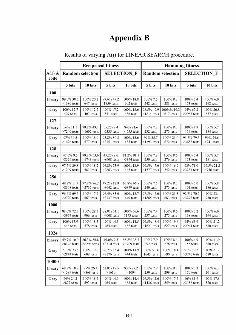
B-1
Appendix B
Results of varying A(i) for LINEAR SEARCH procedure.
Reciprocal fitness Hamming fitness
A(1) &code
Random selection SELECTION_F Random selection SELECTION_F
5 bits 10 bits 5 bits 10 bits 5 bits 10 bits 5 bits 10 bits
100
binary 99.0% 38.5>1380 tests
100% 20.2647 tests
97.6% 47.21859 tests
100% 18.8602 tests
100% 7.5242 tests
100% 8.8283 tests
100% 5.4173 tests
100% 6.0192 tests
Gray 100% 12.7407 tests
100% 12.7407 tests
100% 17.2551 tests
100% 13.6436 tests
98.5% 49.9>1814 tests
100%% 19.3617 tests
94% 67.2>2983 tests
100% 26.8857 tests
127
binary 56% 11.1>7240 tests
99.8% 49.1>1602 tests
55.2% 9.4>7335 tests
84% 81.6>4755 tests
100% 7.2232 tests
100% 8.5273 tests
100% 4.9159 tests
100% 5.7184 tests
Gray 97% 30.5>1426 tests
100% 18.0577 tests
95.8% 80.8>3151 tests
100% 13.6435 tests
99% 35.7>1293 tests
100% 21.0672 tests
91.5% 79.5>3688 tests
99% 24.6>941 tests
128
binary 47.6% 9.5>8529 tests
99.8% 53.6>1743 tests
45.2% 9.6>8908 tests
81.2% 91.1>5374 tests
100% 7.8250 tests
100% 8.6276 tests
100% 5.4173 tests
100% 5.7181 tests
Gray 97.7% 29.8>1299 tests
100% 18.2581 tests
96.8% 75.9>2863 tests
100% 13.9445 tests
99.5% 47.0>1577 tests
100% 16.9542 tests
93% 71.0>3234 tests
99.5% 21.2>756 tests
256
binary 49.2% 11.4>8308 tests
97.8% 76.2>2737 tests
47.2% 12.8>8642 tests
65.8% 66.8>6879 tests
100% 7.5240 tests
100% 8.5273 tests
100% 5.0161 tests
100% 5.8186 tests
Gray 96.4% 69.5>2720 tests
100% 17.7567 tests
96.4% 83.0>3137 tests
100% 13.7440 tests
97.5% 47.0>1865 tests
100% 21.3683 tests
92.5% 70.2>3278 tests
100% 23.4750 tests
1000
binary 88.0% 72.7>3967 tests
100% 28.3906 tests
88.0% 74.1>4008 tests
100% 36.61173 tests
100% 7.4237 tests
100% 8.6275 tests
100% 5.2168 tests
100% 6.0194 tests
Gray 100% 13.9446 tests
100% 18.3578 tests
100% 14.5464 tests
100% 14.5462 tests
99.5% 48.4>1621 tests
100% 19.6627 tests
94% 65.9>2941 tests
100% 21.2680 tests
1024binary 49.9% 10.0
>8176 tests86.3% 86.8>6296 tests
49.0% 9.5>8310 tests
55.8% 35.7>7709 tests
100% 7.9252 tests
100% 8.6278 tests
100% 4.9155 tests
100% 11.9380 tests
Gray 73.0% 73.5>2843 tests
100% 19.0608 tests
96.2% 83.4>3176 tests
100% 13.9444 tests
100% 51.41645 tests
100% 18.4590 tests
91% 79.2>3746 tests
100% 21.2680 tests
10000binary 68.8% 18.2
>1399 tests99% 26.4>868 tests
61.8% 19.5>1610
93% 29.2>1094
100% 7.8250 tests
100% 9.3299 tests
100% 5.3170 tests
100% 6.3201 tests
Gray 96% 24.2>877 tests
100% 18.5593 tests
100% 14.5464 tests
100% 14.4462 tests
99.5% 42.6>1436 tests
100% 17.5559 tests
96% 81.9>3156 tests
100% 17.8570 tests

C-1
Appendix C
Software listing of REMAINDER procedure
procedure REMAINDER(A, B : integer) isR : integer := -1;Cy,Ny: integer := 0;begin --test_procedureif A = 0 thenelseif ( B = 0 ) thenelse
if ( A > 0 ) thenif ( B > 0 ) then
while ( ( A - Ny) >= B ) loopNy:= Ny+ B;R := A -Ny;Cy := Cy + 1;
end loop;else --B<0
while ( ( A + Ny) >= abs ( B ) ) loopNy:= Ny+ B;R := A + Ny;Cy := Cy - 1;
end loop;end if;
else --A<0 --11if ( B > 0 ) then
while ( abs(A + Ny) >= B ) loopNy:= Ny+ B;R := A +Ny;Cy := Cy - 1;
end loop;else
while ( ( A - Ny) <= B ) loopNy:= Ny+ B;R := abs ( A - Ny);Cy := Cy + 1;
end loop;end if;
end if;end if;
end if;PUT ( "Cy = " ); PUT ( Cy );new_line;PUT ( "R = " ); PUT ( R );end REMAINDER;

D-1
Appendix D
Software listing of DIRECT_SORT procedure
with text_io;use text_io;
generictype index_type is (<>);type scalar_type is private;type vector_type is array(index_type range <>) of scalar_type;with function lt (a,b:in scalar_type) return boolean;
package dk_generic_m01aa isprocedure direct_sort(a:in out vector_type;error: in out integer);
end dk_generic_m01aa;
package body dk_generic_m01aa isprocedure direct_sort(a:in out vector_type;error :in out integer) is
stack:array(0..50) of index_type;-- := (others => a'first);j,i,left,right:index_type;p:integer;bottom:index_type :=a'first;top:index_type:=a'last;procedure insert(a :in out vector_type; bottom,top: in index_type) is
x:scalar_type;j:index_type;
beginfor k in index_type'succ(bottom)..top loop
x:=a(k);j:=k;while (j > bottom) and then
lt(x , a(index_type'pred(j))) loopa(j):=a(index_type'pred(j));j:=index_type'pred(j);
end loop;a(j):= x;end loop;
end insert;
procedure partition(a : in out vector_type;bottom,top :in index_type;p,q :out index_type) ismid,i,j:index_type;x:scalar_type;hh:integer;procedure swap(e1,e2 :in out scalar_type) is
t:scalar_type;begint:=e1;e1:=e2;e2:=t;
end swap;begin
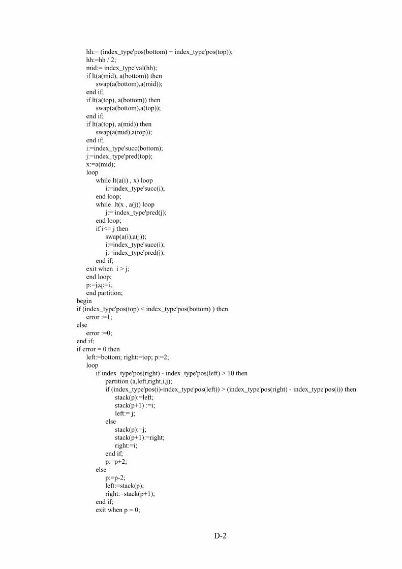
D-2
hh:= (index_type'pos(bottom) + index_type'pos(top));hh:=hh / 2;mid:= index_type'val(hh);if lt(a(mid), a(bottom)) then
swap(a(bottom),a(mid));end if;if lt(a(top), a(bottom)) then
swap(a(bottom),a(top));end if;if lt(a(top), a(mid)) then
swap(a(mid),a(top));end if;i:=index_type'succ(bottom);j:=index_type'pred(top);x:=a(mid);loop
while lt(a(i) , x) loopi:=index_type'succ(i);
end loop;while lt(x , a(j)) loop
j:= index_type'pred(j);end loop;if i<= j then
swap(a(i),a(j));i:=index_type'succ(i);j:=index_type'pred(j);
end if;exit when i > j;end loop;p:=j;q:=i;end partition;
beginif (index_type'pos(top) < index_type'pos(bottom) ) then
error :=1;else
error :=0;end if;if error = 0 then
left:=bottom; right:=top; p:=2;loop
if index_type'pos(right) - index_type'pos(left) > 10 thenpartition (a,left,right,i,j);if (index_type'pos(i)-index_type'pos(left)) > (index_type'pos(right) - index_type'pos(i)) then
stack(p):=left;stack(p+1) :=i;left:= j;
elsestack(p):=j;stack(p+1):=right;right:=i;
end if;p:=p+2;
elsep:=p-2;left:=stack(p);right:=stack(p+1);
end if;exit when p = 0;

D-3
end loop;insert(a,bottom,top);
end if;end direct_sort;end dk_generic_m01aa;

9-1