The Availability Effect: Empirical · PDF filechapter will develop and use an empirical technique to test for the ... blends or combines normative and positive ... As a result, the

This PDF is a selection from an out-of-print volume from the NationalBureau of Economic Research

Volume Title: Doctors and Their Workshops: Economic Models ofPhysician Behavior

Volume Author/Editor: Mark Pauly

Volume Publisher: University of Chicago Press

Volume ISBN: 0-226-65044-8

Volume URL: http://www.nber.org/books/paul80-1

Publication Date: 1980

Chapter Title: The Availability Effect: Empirical Results

Chapter Author: Mark Pauly

Chapter URL: http://www.nber.org/chapters/c11525

Chapter pages in book: (p. 65 - 90)

The Availability Effect:Empirical Results

This chapter has two purposes: first, to compare the "information ma-nipulation" version of the availability effect argument that was developedin chapter 4 with alternative explanations that have been or might be de-veloped to explain the effect. The intent here is to develop suggestionsfor distinguishing empirically between the models, and to spell out thedifferent implications of accepting any particular model. Second, thischapter will develop and use an empirical technique to test for thepresence and causes of the availability effect.

Medical Need, Availability Effect, and the EconomicConcept of Demand

The discussion of the availability effect in almost all of the noneco-nomic literature has implicitly been based on the principle of "medicalneed" or what Fuchs has called the "monotechnic" point of view.1 Inits strongest form this principle asserts that, for any set of preexistingsymptoms or complaints, there is a unique, appropriate, and necessarycourse of treatment, which has unique resource or input requirements.Neither individual preferences nor costs are relevant. For example, thereis a specific set of indications for appendectomy or hernia repair. If theindications are present, the procedure "ought" to be demanded and per-formed. If they are absent, it ought not to be performed. It follows that,for a population with a given distribution of symptoms, there should bea unique number of procedures which ought to be performed, and aunique set of inputs which ought to be used to perform those procedures.While adherents of this view recognize that there may sometimes bevagueness about the necessity of a particular procedure, they do notusually discuss what will or should then determine what is to be done,

65

66 Chapter Five

other than to suggest that additional clinical trials would settle thematter.2

The critical feature of the medical need approach is that what shouldbe done is held to depend only upon the patient's physical and mentalcondition. It follows therefore that if the presence of inputs, of surgicalspecialists for example, is correlated with use when the prevalence ofconditions is known or assumed to be constant, there is prima facieevidence of "demand" or use creation. If surgical rates vary when sur-gical manpower varies but surgically treatable pathology does not, excessresources must be creating "unnecessary" use. Note that this approachblends or combines normative and positive aspects: demand creationoccurs when use varies for reasons for which it ought not.

The economic approaches to be discussed below differ from the med-ical need approach in that they permit use to be determined by morethan just the patient's physical condition and possibly some socioeco-nomic characteristics. In particular, his tastes or desires, the price (realand monetary) that he pays, and the resources at his disposal are heldto be things which affect his use. More than this, there is often the im-plicit normative judgment that, at least in principle and in some situa-tions, these variables ought to affect what he gets. In this approach, then,demand creation requires one to look at both health or condition indi-cators and economic variables before attributing any residual influenceto an availability effect.

Viewed as a positive theory of behavior, the economic approach ismuch less likely to label a given act of behavior as demand creation.Suppose, for instance, a patient has insurance which covers all hospitalcosts. Suppose there is some newly developed, exotic, and expensiveprocedure for which facilities have just been installed and which prom-ises him a positive but slight improvement in his expected health. If thepatient uses that procedure, this would not be regarded as demand crea-tion; it should only be regarded as satisfaction of his (large) demandat a zero price; supply is responding to demand. The installation of theequipment does not create the demand for improvement in health; it isonly the supply response to previously unsatisfied demand. A physicianwould not be acting in the role of agent for his patient if he did notrecommend the procedure. The physician might, especially if he is some-what unorthodox, recognize the true waste involved in this transaction,and so label it the "technological imperative," but it would not be amanifestation of demand creation. If the patient, supposing he were trulyinformed, chose not to have the procedure done, but the physician ma-nipulated information to get the patient's approval, that would be re-garded as demand creation.

67 The Availability Effect

Economic Theories of the Availability Effect

In what follows I will concentrate on availability effects for physi-cians' services. Hospital care will be considered in a later chapter. Thedata will not permit empirical analysis of other types of medical care.

There are four kinds of theoretical explanations of the availabilityeffect to be investigated:

1. The availability effect arises from statistical properties of the esti-mation procedure.

2. The availability effect represents the response of use to changes inthe time or convenience cost of care.

3. Medical services are subject to chronic excess demand, and careis rationed by physicians on the basis of the interest or severity of cases,but excess demand is reduced when the availability of physicians isincreased.

4. Physicians create demand by manipulating the information theyprovide to consumers; when more physicians are present, they alterinformation to induce consumers to use more care.

These explanations are obviously not mutually exclusive. Conse-quently, a test which supports one theory does not necessarily disproveanother. Moreover, because a number of natural theoretical variableswill not be measured (and may not be measurable) directly, proxyvariables will have to be selected. As a result, the failure of an empiricaltest to confirm a theory may only indicate that inappropriate proxyvariables were chosen, not that the theory itself is incorrect.

Data Selection and Statistical Properties

It is clear that trying to estimate a separate availability effect fromaggregate data will involve a severe identification problem. The demandequation of interest is of the general form

(1) QD = D(P,X,Z)

where QD is quantity of some medical input demanded, P is its (user)price, X is a vector of other demand parameters, and Z is a vector ofmeasures of input availabilities. In most demand studies, observationson use per capita and availability have been taken from geographicaggregates.

The problem with such an approach is that not all of the right-handside variables are exogenous, nor is (1) the sole equation determiningobserved use Q. One of the other equations would, for example, be aproduction function:

(2) Q = Q(Z)

68 Chapter Five

If some demand variables are omitted, if supply responds to demand,and if more inputs are needed to supply this output, there will neces-sarily be more use where there are more inputs. But there is no inde-pendent causal effect. Input availability does not cause more use; rather,when people desire more use, more inputs become available.

It has been noted less frequently that ostensible demand creationcould also arise because of measurement error in demand variables.Suppose, as is very common, user price is measured only imperfectly.But suppose that supply responds well to an increase in quantity de-manded induced by a decline in user price. In effect, supply availabilitymay be a better proxy measure of true user price than is measured price.In such a case, price elasticity would be underestimated (because oferrors-in-variables bias) and the demand creation effect would be over-estimated. These problems will tend to be most severe when observa-tions consist of aggregates over the size of a market area (e.g., a stateor SMSA).

In such cases there is likely to be still another source of bias if popu-lation is measured accurately, and data on use and input availability aretaken from the same source. For instance, hospital admissions and hos-pital beds are usually drawn from the same American Hospital Associa-tion survey. But such surveys may omit some possible observations—e.g., the AHA survey omits both Veterans Administration hospital bedsand admissions to such hospitals. Then the coefficient on the independentvariable will again be biased upward as a measure of the effects of inputson total use.

In general, if equation (1) were estimated using actual values of Z, itis clear that the coefficient on Z might be biased upward. This bias mightbe avoided by using predicted values of the Z variables in a two-stageprocedure. But there may still be problems: there may not be an exoge-nous variable in the supply equation with which to identify the demandequation. To see this, consider the most fully specified model, that ofFuchs and Kramer.3 In a technical sense, their approach is free of theomitted demand variable problem because they treat physicians percapita (MD*) as an endogenous variable, and so estimate the demandequation in which MD* enters by 2SLS. They therefore use a predictedvalue for MD* rather than the actual value, and this predicted valueshould be free from correlation with any omitted demand variables.However, the exogenous variables which are used in the first stage topredict MD* are either explicitly demand variables, or, what is moreserious, they are variables which might not really be exogenous, butrather would themselves be correlated with the omitted demand vari-ables.

For example, one of the most important variables in the MD* equa-tion is hospital beds per capita. But as was argued above, and as will be


developed in more detail in chapter 6, it seems more reasonable to sup-pose that beds and physician time are jointly demanded to producehospital output. Neither physicians nor beds are exogenous. This effectis even stronger in the Fuchs-Kramer study, since interstate variationin their measure of physician visits per capita (the dependent variablein the demand equation) depends strongly on variation in hospital bed-days per capita, because physician hospital visits are estimated by usingthe number of bed-days. For both of these reasons, it is likely that muchof the positive relationship between MD* and beds arises from theirmutual dependence on omitted demand variables. The other importantpredictor of MD* is the number of medical schools in the state (notmedical schools per capita, or per physician; apparently medical schoolsare a public good as far as physicians are concerned). It would againappear to be a reasonable conjecture that, if more medical schools in astate do mean more physicians, those states with unusually high demandsfor physicians' services would be expected to have more medical schools.Again, this variable could be correlated with omitted demand variables.

This is a specific illustration of the general difficulty of finding "trulyexogenous" supply variables for a product whose output does not dependon weather or geography. A better choice would have been some deter-minants of real physician income, such as temperature, extent of urbanamenities, or golf courses per capita, or possibly some measures of gov-ernmental restrictions on physician flow. Fuchs and Kramer did trysome of these variables, but apparently they were not strongly related toMD. In a more recent study of the demand for surgical services, Fuchswas able to relate the surgeon stock to hotel expenditures per capita asa proxy for locational desirability.4

One way to mitigate these problems is to avoid aggregated data. Thatis, instead of using per capita demand in a market area, which is surelygoing to be related to area-wide levels of omitted variables, one coulduse as observations the quantities demanded by individuals. It is lesslikely that the number of physicians will respond appreciably to unusu-ally high or low demands by a single individual. One can only say lesslikely, not unlikely, since it is possible that any omitted variables mightaffect all persons in an area in a similar way. If, for instance, all oralmost all people in South Dakota have unusually low demands forphysicians' services, perhaps because of a common ethnic background,then the omitted variable problem returns. If however, the variancewithin areas of some characteristic is sufficiently large, and especiallyif it is large relative to the variance across areas, input availability cansafely be treated as exogenous to a given individual. For these reasons,and also because of other desirable aspects of the data, individual obser-vations will be used in the empirical analysis which follows.

70 Chapter Five

Nonmoney Price and the Availability Effect

There is one omitted demand variable which should be given specialattention. Suppose the number of physicians in an area is increasedexogenously. The money price of their services may fall. But, in addi-tion, the time and inconvenience cost of seeing a physician is likely tobe reduced. Distances will be shortened, the possibility of waiting inqueues reduced, and so on. As Acton5 has shown, the time cost ofambulatory physicians' services may be large relative to the money priceor cost. Consequently, even with money price held constant, an altera-tion in input availability may have a substantial effect on use if it affectsthe time cost of care. (Quality might also be affected.)

It may be possible to construct a test to suggest whether the avail-ability effect arises from a change in the time cost of care. Let the totalprice of a unit of care be given by

(3) P = PM+Wt

where PM is the (user) money price, t is the time spent per unit of careobtained, and W is a measure of the opportunity cost of time.

Suppose all buyers wait approximately the same length of time. Sup-pose that increases in physicians per capita reduce waiting time by thesame amount for all persons. Newhouse and Phelps6 have shown that

(4) y)•"» - PM + wt -

where r}qt is the elasticity of demand with respect to time and e is theelasticity of demand with respect to total (money plus time) price. Itfollows directly that changes in physician stock will reduce time cost bya larger amount for high wage persons. Since time cost is a larger frac-tion of total cost for high wage persons, equation (4) implies that, if e isthe same for all persons, the elasticity of use with respect to physicianstock r]qm will vary positively with W. While it is likely that higher wagepersons will seek medical care which has a higher money cost and alower time cost, it seems reasonable to suppose that money cannot besubstituted for time to such an extent that total time cost will be less.(If PM equalled zero for a low-income person, then r)qt would equal e,and would be greater than r)qt for other persons. However, persons inhouseholds with incomes low enough to make them eligible for Medicaidare omitted from the sample that will be used.)

Since in practice W and income often vary together, and e may de-cline with income, availability elasticities may not differ significantly.In the empirical work, I shall make some attempt to control for incomewhile W varies. Note finally that if, instead of being constant elasticity,the demand curve is assumed to be approximately linear in P and q,


then € will increase as W (and P) increase, making the predicted vari-ation in 7]qm with W even more likely.

Time cost may also be relevant for understanding differences in theavailability effect between urban and rural areas. It is often alleged thatthere is a relative "shortage" of physicians in rural areas. Indeed, theper capita number of physicians is substantially less in such areas. Timecost may therefore be high in such areas. If time cost is higher in ruralareas and if relative money prices are the same in rural and urban areas,a given percentage change in physician stock should produce a largerpercentage change in total price in rural areas. To the extent that theavailability effect operates through a change in time cost, the elasticityof use of care with respect to physician stock would therefore surely bepositive and probably greater in rural than in urban areas. While nominalmoney prices are lower in rural areas, so is the cost of living, so thatrelative prices may be sufficiently uniform to permit this test.

Excess Demand

Excess demand exists when the quantity demanded of some serviceexceeds the quantity supplied at a given price. If excess demand forphysicians' services exists at current prices, it is possible that an increasein supply of physicians may cause the observed quantity used to increasewith no change in money prices. The case is clearest and neatest whenexcess demand occurs because of price controls imposed on exogenouslydetermined input supplies. If price is below the market-clearing price,quantity supplied will fall short of quantity demanded. Now let there bean exogenous increase in inputs available to produce care (physicians,beds). The quantity used at the fixed price will increase: this might becalled an availability effect.

Of course, if price controls exist everywhere (though at differentprices below the equilibrium one), the "demand" elasticity that will beobserved empirically will have the wrong sign, since the estimated rela-tionship will actually represent points on a supply curve. If price controlsexist in some places from which observations are taken but not others,one may observe both a negative demand elasticity and an "availabilityeffect," neither of which will be accurately measured.

The price control model is not very realistic, since, except for theEconomic Stabilization Program and some kinds of Blue Shield reim-bursement mechanisms (now largely disused), prices are not fixed. Onecan argue that if prices respond slowly to excess supply or demand, theactual situation may approximate price controls. But this leaves theuncomfortable questions of why prices respond so slowly, and whetherone observes equilibrium or disequilibrium in a cross section.7

72 Chapter Five

A more complete answer is provided by arguing that there are reasonswhy the price might stay below the market-clearing level. All of thesereasons involve entering either the magnitude of excess demand or theprice itself in the provider's utility function. In what follows I will firstconsider alternative theories of physician behavior that might be con-structed to explain the existence of permanent excess demand.

Feldstein8 was the first economist to suggest that physicians may getutility from excess demand; this was one of his explanations for theupward slope of his estimated "demand" curve for physicians' services.(He also argued that lower prices give physicians utility.) The notion isthat physicians maintain a queue in order to be able to select "interest-ing" or urgent cases.

Feldstein appealed to the existence of a chronic doctor shortage since1946 as evidence for the existence of such utility functions. Exactlywhat the evidence is for this shortage, and its dimensions, was nowherestated. However, it will still be useful to present a model of equilibriumnonprice rating.

I assume that each physician has a utility function of the form U — U(Y,a ) where Y is money income and a is the fraction of total casesseen that is regarded as interesting. I assume that hours of work arefixed at L, and that output (number of cases seen) depends only onhours of work. Each physician is assumed to be confronted with a pro-rata share of the market demand curve. Of the total demand (or perphysician demand) at each price, the fraction otD of cases is interesting.However, the physician is assumed to be unable to charge differentprices for interesting and uninteresting cases. For example, it may notbe possible for the patient (or physician) to identify beforehand whichinitial visits will be for interesting conditions. Thus, if each physiciansets price at the level which clears the market at QD = Q8 = Q(L),then <x = aD. However, if physicians value interesting cases, they maybe willing to reduce prices below the market clearing level. That is, theonly way to induce demand for initial and subsequent visits for interest-ing cases may be to set an initial price below the market-clearing level,and then select interesting cases from the queue thus generated. Themarginal equilibrium condition here (holding quantity supplied Qs con-stant) is:

where Ua is the marginal utility of the proportion of interesting cases,and UY is the marginal utility of income. It is easiest to explain thiscondition by considering a small change in price. The benefit from re-ducing price by one dollar is a gain in the fraction of interesting cases


of aD—=r= . But the cost is a reduction in income of Q&. The physicianUs

will create excess demand for his services as long as the benefit fromdoing so exceeds the cost.

Since the cost of cutting price by one dollar, or Q8, is positive foreven the initial price reduction from the market-clearing income-maxi-mizing level, it is possible that a physician who values interesting casesmay still decide not to cut the price. The cost may just be too high. Butif he does decide to cut price, the effects of such behavior may be toincrease his utility, and price may settle to some value below the market-clearing price. Now let the number of physicians be increased. If priceis held constant and if a is held constant, income will decline. If a is anormal good, each physician will reduce his desired level of a by draw-ing down his queue. (The initial price is likely to no longer be theequilibrium price.) Total output will increase, but the increase in outputwill consist entirely of uninteresting cases. This discussion shows a wayof determining whether any observed availability effect may be attrib-uted to this cause. In particular, the elasticity of use with respect to thenumber of physicians per capita should be less for cases labeled asinteresting, or for persons with such cases, than for uninteresting cases.

The "interest" or "severity" on the basis of which rationing occursis, of course, that which is perceived by the physician. Insofar as thereare a priori reasons why physicians and patients might differ in theirestimates of severity for particular kinds of cases, then another test ofthis kind of theory would involve determining whether the response forthose kinds of cases which physicians do not deem to be severe is largerthan for those cases which physicians do regard as severe. Such a testwould require proxy ing severity by symptoms or by diagnosis, or byphysician and patient attitudes toward symptoms and diagnosis.

Alternative bases for rationing other than severity yield alternativepredictions about differences in the availability effect. It is possible, forexample (as also suggested by Feldstein), that excess demand may ariseif price enters the physician's utility function. Suppose demand increasesfor a type of care for which a critical physician input is in perfectlyinelastic supply. A price rise could reequate demand and supply, butphysicians may recognize that its only function is to transfer income frompatients to physicians. Accordingly, they may neglect to raise prices, andration on the basis of severity or interest. But the higher patients' in-comes are relative to physicians' incomes, the less this kind of benev-olent rationing is likely to occur. Thus one would predict that theresponse of use to availability should differ by severity, but that thesedifferences should be greater the lower the relative incomes of patients.If severity itself enters the physician's utility function, there would beno such difference.

74 Chapter Five

The precise determination of whether excess demand exists or not isdifficult because queues do not necessarily mean that price is too low,any more than the existence of inventories means that the price is toohigh. When demand is stochastic, a profit-maximizing firm may chooseto hold inventories, or to permit queues to develop; either way the pro-duction process is smoothed out. Which strategy is chosen depends,roughly speaking, on which is cheaper. Having groceries wait for peoplein the supermarket rather than vice versa makes sense if the costs ofmaintaining inventories are less than the costs of delay. Having peoplewait for doctors rather than vice versa makes sense if the cost of doctors'time exceeds that of the cost of patients' waiting time. What is actuallychosen is some mix of queues and inventories: there are occasionaldelays at the supermarket, and doctors sometimes have time for a cupof coffee. // prices could be adjusted with this variation in demand,some (but probably not all) queues would disappear; but such adjust-ment is probably itself too costly. One can be certain that excess demandexists only if there is always a queue, and it is not clear that this obtainseven for "busy" doctors.

One final question is whether the behavior predicted by these theoriesmight also be predicted by, or at least consistent with, long-run profit-maximizing behavior on the parts of physicians. Unfortunately for thepurposes of hypothesis testing, the answer seems to be yes.

It may be, for instance, that most people have a kind of implicit con-tract with their physician. Because it is too costly to vary prices withurgency and demand, the physician agrees to let the patient jump thequeue at no increase in price for serious illness if the patient will wait(patiently?) in the queue when the complaint is nonurgent. This permitsthe physician to even out his patient flow, thus increasing his produc-tivity and lowering the price he needs to charge. Thus it is possible toconcoct a profit-maximizing explanation of both (1) the regular doctorand (2) taking the most serious cases first. Hospitals will do the sameif they do what physicians want.

Measuring Information Manipulation

In the information manipulation theory, the demand equation of in-terest has the general form

where QijD is the quantity of a given medical service demanded by per-

son i in area /', Pi} is the user price (net of insurance) paid by person i,X1 is a vector of person /'s demand characteristics (including his state ofhealth, and Aj is the level of accuracy he experiences. It is assumed thatAj is the same for all persons in a given area.


It will be possible to obtain reasonable approximations of QD, P, andX. But A cannot be measured directly. Instead, as suggested by theearlier discussion, the level of accuracy chosen by the representativephysician will depend upon the gross price level, the quantity that eachphysician can sell at that price, and the level of the physician's subjec-tive marginal opportunity cost. I will assume that the marginal costcurve is the same for all providers. With gross price Pj held constant,total quantity demanded in an area depends on the mean area-widevalues Xj of the demand parameters (including others' insurance cover-age). The demand per physician then depends on the number of physi-cians. Thus we can write:

(2) A* = A (F, MD**, X*)

where MD*j is the stock of physicians per capita in area / and P} is thegross price received by physicians in area /. Note that A is greater thelarger the demand per physician. So while an individual's demand forphysicians' services would be greater the sicker he is, it would be smallerthe sicker everyone else in his community is, because in the latter casethe physician would have less incentive to create demand.

Substituting the equation for A into the demand function gives

(3) QDV = Q(P*i, X\ X\ MD*>, Pi)

Since P** = INSlPj, where INS* is the fraction of /'s expenditure notcovered by insurance, the actual estimating equation will be

(3') Q% — Q(INS\ P\ X\ X*,

Since Pj has effects on consumer demand both directly through the userprice and indirectly through incentives for demand creation, it is notdesirable to impose the constraint that changes in INS1 and Pj whichhave the same influence on P*j should have the same influence on de-mand. In particular, changing Pij by changing INS1 should have a largereffect on quantity demanded than that from changing Pj, since changesin the prices paid to physicians provide offsetting incentives to createadditional demand. In the data to be used there is no measure of themarginal or average fraction of expense covered by insurance, only anindication of whether or not the individual is covered by hospital and/ormedical-surgical insurance. A dummy variable for INS is therefore usedin the regressions. This procedure is equivalent to assuming that allpersons who have insurance have the same coverage.

Target Income

A final kind of theory that contains elements of all of the precedingones is the so-called "target income" theory. This theory was first sug-

76 Chapter Five

gested by Newhouse and Sloan,9 but has received its most extensivedevelopment by Evans.10 In its simplest and most naive form, the theoryassumes that physicians have target money incomes and target work-loads they wish to achieve. Both are chosen with reference to what isacceptable or usual in the community and in the profession. Productivityand the level of other inputs held constant, the target workload deter-mines output Q. Given input prices and Q, the physician then choosesthe gross output price that achieves the target income. If the Q chosenin this way exactly equals the Q corresponding to this gross price onsome market demand curve, then demand is just satisfied. If Q is lessthan the quantity demanded, excess demand prevails. If Q is greaterthan the quantity demanded, actual Q will be increased as physicians"order extra work for patients, perform unnecessary or marginally neces-sary operations, or recall patients for extra visits."11 Increases in thenumber of physicians will in either case result in an increase in actualQ at any price—an availability effect will be observed.

In its simplest version, the target income theory is consistent with anavailability effect which arises either from the drawing down of excessdemand or from demand creation. It simply makes observed demanddepend on the number of physicians. If a distinction is to be made be-tween a target income theory and any other theory, that distinction mustbe based on a presumed fixity in the incomes, real or money, that physi-cians desire.

If desired or target income is assumed to be fixed, the theory makesa definite qualitative empirical prediction which permits it to be distin-guished from maximizing models. It predicts that an exogenous increasein gross price will lead to a reduction in the quantity of services percapita supplied and used. For if quantity were held constant, then in-come would rise. To keep it at the target level, quantity must fall.12

The information-manipulation theory, however, is consistent with thefinding of a positive or zero effect if the substitution effect of a priceincrease (which represents a greater reward for more business) offsetsthe income effect.

While Evans seemed initially to support the naive target income the-ory,13 his "more extended model" allowed actual workload to departfrom desired workload. More importantly, he allowed desired work-loads to be a positive function of price, which makes it possible for priceand quantity used to be positively related. He used casual empiricism onthe Canadian experience to suggest that the relationship will still usuallybe negative, but the "extended" theory as such cannot be refuted. In-deed, as Sloan and Feldman have shown,14 any outcome with respect tothe relationship between physician stock and price or aggregate usewould be possible under the "extended" theory.


These alterations make Evans' models indistinguishable from the de-mand creation model discussed in chapter 4; they rob the target incomeapproach of any distinctive qualitative empirical predictions. In orderto preserve this distinction, in what follows I shall regard the targetincome approach as the initial, naive model. Evans' "more extendedmodel" will instead be identified with the information manipulationtheory.

Data Sources and Variable Measurement

In this section some empirical tests of alternate theories of the avail-ability effect will be provided. The basic source of data on individualuse and individual characteristics is the 1970 Health Interview Surveyof the National Center for Health Statistics.15 This survey consists of theresults of a questionnaire administered to about 110,000 persons in39,000 families on their health, use of medical care during the pastyear, and socioeconomic characteristics, including insurance coverage.From A.M.A. and A.H.A. data sources, I obtained information on thenumber of physicians of various types, hospital beds, and gross pricesof hospital and physician services in the "primary sampling units"(PSUs) from which the sample was drawn. PSUs are counties, groupsof counties, or SMS As. For 22 large SMS As that are identified on thetape, the actual values of the PSU-level variables could be used. For theother PSUs the National Center for Health Statistics attached a set ofdecile rank orders of each of the variables to each of the PSU codes.I then substituted for the decile rank orders the population-weightedmean values of each of the variables for each combination of decilerank orders. In most cases, this procedure will associate a unique set ofvalues for the area variables with each PSU. The variables used in theempirical work are as follows:

Dependent Variables

Three measures of utilization:1. Physician visits, last 12 months. This includes telephone calls but

excludes visits to hospital inpatients. Because of the recall period, theremay be some error in measurement.

2. Hospital episodes, last 12 months, in nonfederal, short term hospi-tals.

3. Average stay per episode (equals hospital days divided by hospitalepisodes).

Independent Variables and Abbreviations

Personal Variables:1. Restricted activity days, last two weeks (RAD).

78 Chapter Five

2. Number of chronic conditions (CONDS).3. Age (AGE).4. Sex, 1 if female (SEX).5. Female of childbearing age dummy (F15-44).6. Family size (FAMSZ).7. Work status: whether individual is currently employed or not

(WORKING).8. No insurance coverage (NOINS): indicates whether the indi-

vidual is covered by hospitalization or surgical insurance orMedicare or not. About half of the surveyed families wereasked this question, so in most of the analysis only observa-tions on persons who were asked this question were used.However, restricting the data set to families who answered thequestion would lead to small cell size for the high educationgroup in all but the large metropolitan areas. Accordingly, aninsurance coverage variable is not included for high educationfamilies in other metropolitan or rural areas.

9. Family income in 100's (FAMINC).PSU Variables:

10. Office based M.D.'s per 100 persons (OBMD*).11. Surgical specialists as a fraction of office-based M.D.'s (SURG/

MD).12. General practitioners as a fraction of office-based M.D.'s (GP/

MD). The variables GP/OBMD and SURG/OBMD measurethe proportion of total office-based physicians who are generalpractitioners and surgeons respectively. They capture any dif-ferences in the quality or characteristics of a typical patientvisit, as well as differential specialty effects, if any, on demandcreation.

13. Hospital based M.D.'s per 100 persons (HBMD*)—mainlyresidents, interns, and other hospital-salaried physicians.

14. Nonfederal short-term hospital beds per 100 persons (BEDS*).15. Hospital cost per patient-day for nonfederal short-term hospi-

tals in the PSU (HOSCOST).16. Population density (POPDENS).17. Physician office visit fee (MDFEE). Two measures are used.

The fee measure used for all areas is the fee screen for Medicare pa-tients for followup office visits. This screen is supposed to represent theseventy-fifth percentile of the prevailing distribution of fees in variousgeographic areas. However, since different procedures are used by dif-ferent carriers to set up the fee screen, the accuracy of this measure isunknown. When there were different fees for general practitioners andspecialists, a weighted average was used. For the 100 largest SMSAs,Mathematica, Inc. conducted a telephone survey in 1973 to ascertain


the fee for a routine office visit to a primary care practitioner,16 and thismeasure should be an accurate index of fee levels for such services.Accordingly, results for office visits for the 22 largest cities are presentedusing the Mathematica prices as well as using the Medicare fee screens.

In principle, cost-of-living differences should be taken into accountin estimating monetary variables (income and fees). A complete set ofsuch indexes is available from the Bureau of Labor Statistics only forthe large-city subsample, not for all other cities or for rural areas. Acomparison of regressions using undeflated and deflated data for thelarge city subsample will suggest whether the absence of deflation biasescoefficients on the variables of interest.

Classification of Results for Physician Visits

Results for physician visits are presented for several different datasets. First, persons are classified by the number of physicians in themarket area in which they live: the 22 largest SMS As, in which it wouldprobably be very difficult for consumers to get reliable information onany individual physician; nonmetropolitan areas, in which such informa-tion is presumably easier to obtain; and other, smaller metropolitanareas, which might be expected to be intermediate.

The information manipulation theory would suggest that availabilitymight have a greater influence in those large metropolitan areas in whichindividuals have difficulty determining the quality or accuracy of theadvice which any individual physician provides. An excess demand the-ory, on the other hand, would predict that availability effects would bemost likely to be observed in rural areas, where physician stock is low-est and excess demand presumably the greatest.

Second, results are presented for persons in households in which theheads have different levels of education. Education level is intended tobe a proxy for the prior stock of information. In most of the analysis,results will be presented for two extremes of the distribution of educa-tional attainment—persons in households in which heads are not highschool graduates (low head education) and persons in households withheads with college degrees or better (high head education)—for thereasons discussed in chapter 4.

Where an availability effect is detected, the sample is further subdi-vided in ways which, it is hoped, correspond to differences suggested byother theories of the availability effect. The survey did not ask aboutwage income or hours, but it did ask whether or not the person wasemployed. It would seem reasonable to suppose that, money incomeheld constant, adults who are working have a higher time cost thanadults who are not. Another method of division is by number of chronic

80 Chapter Five

conditions, which may serve as proxy for illness severity or physicianinterest in the case.

Two alternative methods of estimation were used. Since there is aconcentration of observations at zero, especially for the low educationgroup, ordinary least squares regression on all observations would yieldincorrect estimates. Tobit regression is usually the appropriate techniqueto be used.17 However, there are reasons to fear that tobit may not betheoretically appropriate for the question being investigated here, as hasbeen suggested by Newhouse and Phelps.18 Physician advice can onlyinfluence use if the consumer first contacts the physician to seek hisadvice. The initial decision to seek advice should not be influenced byphysician information; although physician availability may influence thisdecision, it will do so through changes in nonmoney price. Once a per-son has made at least one visit, then he will potentially have receivedsome physician advice and be subject to an information effect. Accord-ingly, analysis of the subsample of persons with positive doctor visits ismore likely to display an information effect than is analysis of the totalsample. Of course, not all of the persons with positive numbers of visitswill have been subject to information manipulation; there may be severalinitial visits, for a series of illnesses, included in the data. Moreover, thecensoring issue discussed earlier suggests that those with positive visitsmay be more susceptible to information manipulation than those withno visits. Nevertheless, the set of those with positive visits may still bemore appropriate for investigation of an availability effect than the fullsample. Such analysis of nonzero observation can be done using OLS,since there is less of a concentration of observations at a lower limit.

Two kinds of person are omitted from the sample. Persons withhousehold incomes below a poverty line are dropped because their useis likely to be covered by Medicaid and so not responsive to changes infees. Those with more than 52 physician visits in a year are also droppedin order to avoid bias from extreme values.

The full specification described in the section "Measuring InformationManipulation" indicates that area demand variables as well as individualdemand characteristics should be included in the equations. Several sucharea demand variables—percentage of population covered by Medicare,percentage of under-65 population with private health insurance (forthe state in which the SMSA is located) and percentage of populationunder age 5—are available for the 22 large cities. Accordingly, resultswith regressions which include these variables are also presented.

Empirical Results: Physician Ambulatory Visits

The primary prediction of the information-manipulation theory is thatalterations in accuracy should have less effect on those with sufficientlylarger prior stocks of information. There are two primary proxies for


incentives for alterations in accuracy suggested by the theory: the num-ber of physicians per capita, and the gross price of a unit of output.

The two major questions of interest are: (1) whether availabilityeffects are shown and (2) if effects are shown, whether they differ acrosseducational groups. Table 5.1 shows the coefficients for OLS regressionsof physician visits during the preceding 12 months for persons with posi-tive physician visits. Different regressions are presented for persons inthe two separate education groups and in three different geographicareas; means and standard deviations are shown in appendix table 1.Table 5.2 presents similar tobit regressions on the full sample of persons.For the reasons discussed above, the availability effect is most likely tobe observed in the positive visits sample, and so these results will bediscussed first.

Availability variables

The three availability variables are OBMD*, HBMD* and BEDS*.OBMD* has a significant and positive coefficient for the low educationgroup in two out of three geographic areas. The size of the coefficient(and the elasticity) is much larger in the large urban areas than in therural areas. For high education families, however, the coefficient onOBMD* is negative and significant for the large urban areas, and insig-nificant elsewhere. HBMD* tends to have the same sign as OBMD*, butto have a lower significance level. BEDS* is not usually significant.Application of an F-test for differences in the sets of coefficients acrosseducation groups finds that the set of coefficients on the two educationgroups is significantly different in all three area subsamples. In addition,the coefficients on OBMD* and HBMD* do differ significantly betweenthe low and high education regressions in two of the three areas.

The remainder of the area variables are occasionally significant, butthere is no consistent pattern. The proportion of physicians who areG.P.'s does not affect the ambulatory visit rate, while the proportionwho are surgical specialists tends to depress the rate, but to a significantextent only for high education families. While none of the coefficientsdiffers significantly across education groups, there is some weak evidencethat surgeons may substitute away from ambulatory care toward hospitalcare. However, the results for the effect of surgeons on hospital use, tobe presented later, do not confirm this suggestion. Another plausibleexplanation is that surgical specialists treat conditions with fewer ambu-latory visits even when they do not substitute inpatient hospital stays.The physician's fee is not significant for high education families, butdoes have a significant and positive effect for the low education familiesin smaller metropolitan areas.

Other demand variables have generally expected coefficients. Bothrestricted activity days and number of chronic conditions are stronglyrelated to the doctor visit rate. Older persons tend to make more visits

82 Chapter Five

as do females in general (in low education families) and females ofchildbearing age. Family size has a slight tendency to reduce the visitrate, while workers make fewer visits than nonworkers.

These results are consistent with the information manipulation theoryof the availability effect. When an availability effect is observed, it ispositive and significant for the low education families in two out of threeareas. (The negative and significant effect of OBMD* for high educationfamilies in large cities may reflect a change in the quality or character ofa visit when physicians are more plentiful.) There is also a positive andsignificant effect of price on use for low education families in the other

Table 5.1

IndependentVariable orStatistic

RAD

CONDS

AGE LT 15

AGE 45-64

AGE 65 +

SEX

F 15-44

FAMSZ

WORKING

NOINS

FAMINC

GP/MD

SURG/MD

POPDENS

MDFEE

Physician Visits Regressions: Persons with Some Physician Visits(ordinary least squares)

Regression Coefficients (/ statistics in parentheses)

22 Largest SMSAs

Low HeadEducation

.176(4.15)2.21

(17.4)-.304

(-0.73).986

(2.55)2.45

(5.01).599

(2.16).636

(1.39)-.066

(-0.97)-.712

(-2.54)027

(0.08).001

(0.30)3.03

(0.56)—7.00

(-0.64).019

(1.09)-.125

(-0.80)

High HeadEducation

.280(4.69)1.81

(12.3)-.429

(-0.97).061

(0.14)1.78

(2.68).229

(0.70).919

(1.90)-.064

(-0.88)-1.33

(-4.14)QQ4

( 2.02)-.004

(-2.55)-7.14

(-1.60)-16.6(-1.66)

.007(0.38)

.126(0.73)

Other SMSAs

Low HeadEducation

.067(1.59)1.60

(13.8)-.140

(-0.35)1.00

(2.72).722

(1.53).510

(1.93).849

(1.97)-.052

(-0.89)-.965

(-3.67)350

( 1.26).002

(0.95)2.40

(1.09)-5.89

(-1.35)-.029

(-0.95).178

(2.59)

High HeadEducation

.212(3.90)1.63

(13.8)1.18

(3.45).172

(0.42)1.83

(3.65)-.101

(_0.40)1.51

(4.02)-.190

(-3.39)-.095

(-0.60)

-.0001(-0.03)

-.281(-0.12)-1.21

(-0.28)-.052

(-2.12).009

(0.15)

NonmetropolitanAreas

Low HeadEducation

.263(6.93)1.60

(15.7)-.376

(-1.07)1.06

(3.19).901

(2.09).451

(1.91)1.20

(3.10)-.071

(-1.23)-.620

(-2.63)e-tn

(2.19).0003

(0.27)1.54

(1.37)-.551

(-0.28).173

(2.62)-.043

(-0.28)

High HeadEducation

.370(6.54)

1.50(12.83)

.304(0.83)

.254(0.70)1.00

(1.88)-.455

(-1.74)1.38

(3.48)-.230

(-3.66)-1.05

(-3.89)

-.001(-0.76)-1.89

(-1.63)-4.63

(-2.09)-.053

(-0.76).010

(1.14)


Table 5.1—continued


HOSCOST

BEDS*

HBMD*

OBMD*

Constant

n

F statistic forhypothesis ofinequality ofregression co-efficients.

Regression Coefficients (t statistics in parentheses)

22 Largest SMSAs

Low HeadEducation

- .025(1.79)

-2.29(-0.87)

14.0(1.59)32.0(3.02)4.38

(0.65).1693461

(F.oi [19, large n] = 1.8

High HeadEducation

.019(1.28)-.370

(-0.15)-18.3(-1-93)-25.8(-2.44)

12.18(2.22)

.1402189

2.38

18.)

Other SMSAs

Low HeadEducation

-.019(-1.74)-1.13

(-0.95)4.89

(0.88)-.902

(-.134)4.96

(1.73).123

2545

High HeadEducation

- .003(-0.42)-2.13

(-2.12)-.945

(-.197)3.55

(0.56)4.59

(1.78).1013184

2.46


Low HeadEducation

.025(2.56)-.968(2.62)3.59

(1.16)5.79

(2.53).523

(0.13).1733128

High HeadEducation

.045(0.78)

.611(1.04)

-7.93(-2.88)

.771(0.62)5.31

(3.92).131

2562

2.85

NOTE: Means and standard deviations are shown in appendix table 2.

Table 5.2


RAD

CONDS

AGE LT 15

AGE 45-64

AGE 65 +

SEX

F 15-44

Physician Visits Regressions: All Persons(Tobit Regressions)

22 Largest SMSAs

Low HeadEducation

High HeadEducation

Other SMSAs

Low HeadEducation

High HeadEducation


Low HeadEducation


.506(8.51)4.05

(21.6)1.59

(2.90)0.55

(1.10)1.72

(2.70).748

(2.05)2.05

(3.43)

.488(6.45)3.32

(15.4)1.37

(2.50)0.66

(1.26).825

(1.00).093

(0.23)2.70

(4.47)

.349(7.49)2.82

(19.5).082

(0.19).091

(0.23)-.464

(-0.92)1.12

(3.94).395

(0.85)

.404(4.15)2.76

(13.4)1.76

(3.06).015

(0.03)1.16

(1.39).197

(0.46)1.93

(3.05)

.566(9.02)3.44

(19.0).954

(1.73).129

(0.25)-.072

(-0.11).770

(2.07)2.67

(4.39)

High HeadEducation

.566(7.27)2.81

(15.5)1.69

(3.48).263

(0.55).052

(0.07)-.777

(-2.21)2.60

(4.88)

84 Chapter Five



FAMSZ

WORKING

NOINS

FAMINC

GP/MD

SURG/MD

POPDENS

MDFEE

HOSCOST

BEDS*

HBMD*

OBMD*

Constant

Significanceof chi-squarestatisticn

22 Largest SMSAs

Low HeadEducation

High HeadEducation

Regression Coefficients

-.332(-3.62)

-.173(-0.47)

9 1 9

(-0.55).011

(3.44).800

(0.12)-6.09

(-0.43).042

(1.83)-.363

(-1.80)-.066

(-3.57)-8.87(2.63)30.7(2.62)45.7(3.31)6.06

(0.70)

.000

5005

-.262(-2.74)-1.58

(-3.83)1 76

(-3.19).000

(0.04)-7.78

(-1.40)-8.81

(-0.71).023

(0.87)-.327

(-1.51).018

(0.97)-5.98

(-2.07)10.15(0.85)

— 3.79(0.28)8.15

(1.18)

.000

2693

Other SMSAs

Low HeadEducation

High HeadEducation


Low HeadEducation

(/ statistics in parentheses)

-.209(-2.84)

-.811(-2.83)

1?1

(-0.39).009

(3.71)1.60

(0.66)-3.60

(-0.75).011

(0.35).047

(0.53)-.010

(-0.93)-.059

(-0.05)2.40

(0.39)6.78

(0.95)-.225

(-0.07)

.000

3864

-.261(-2.76)

-.213(-0.49)

.003(1.15)

-2.89(-0.80)-3.51

(-0.49)-.067

(-1.70)-.116

(-1.16).016

(1.08)-1.34(0.78)2.73

(0.14)-.023

(-0.00)2.81

(0.67)

.000

3950

-.257(-2.89)

-.304(-0.81)

1 59(-4.31)

.002(0.50)

-1.09(-0.60)-5.71

(-1.85)-.008

(-0.94)-.004

(-0.31).005

(2.82)-.525

(-0.45)-3 .20

(-0.65)2.21

(0.26)-2.56

(-1.14)

.000

4927

High HeadEducation

-.331(-3.76)-1.04

(-2.85)549

(2.05)-.002

(-0.98)-.481

(-0.30)-.612

(-0.20)-.119

(-1.69).143

(1.95).006

(0.51).705

(0.90)-9 .04

(-2.38)-.754

(-0.46)1.49

(0.50)

.000

3323

NOTE: Means and standard deviations are shown in appendix table 1.

metropolitan areas, again offering evidence for demand creation (butagainst the naive target income theory).19

It is also worth noting that, although there is an availability effect forlow education families in rural areas, that effect is much smaller thanin large urban areas. Since rural areas are supposed to be areas of great-est physician "shortage," one could conclude either that the shortage isrelatively mild, or that the potential for demand manipulation in suchareas is limited by better consumer information on the accuracy of in-formation provided by individual physicians.


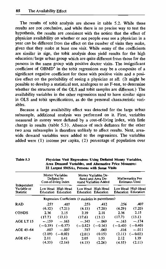
The results of tobit analysis are shown in table 5.2. While theseresults are not conclusive, and while there is no precise way to test thehypothesis, the results are consistent with the notion that the effect ofphysician availability on whether or not people ever see a physician in ayear can be different from the effect on the number of visits they make,given that they make at least one visit. While many of the coefficientsare similar in sign, the tobit analysis does yield results for the higheducation/large urban group which are quite different from those for thepersons in the same group with positive doctor visits. The insignificantcoefficient of OBMD* in the tobit regressions may be a composite of asignificant negative coefficient for those with positive visits and a posi-tive effect on the probability of seeing a physician at all. (It might bepossible to develop a statistical test, analogous to an F-test, to determinewhether the structures of the OLS and tobit samples are different.) Theavailability variables in the other regressions tend to have similar signsin OLS and tobit specifications, as do the personal characteristic vari-ables.

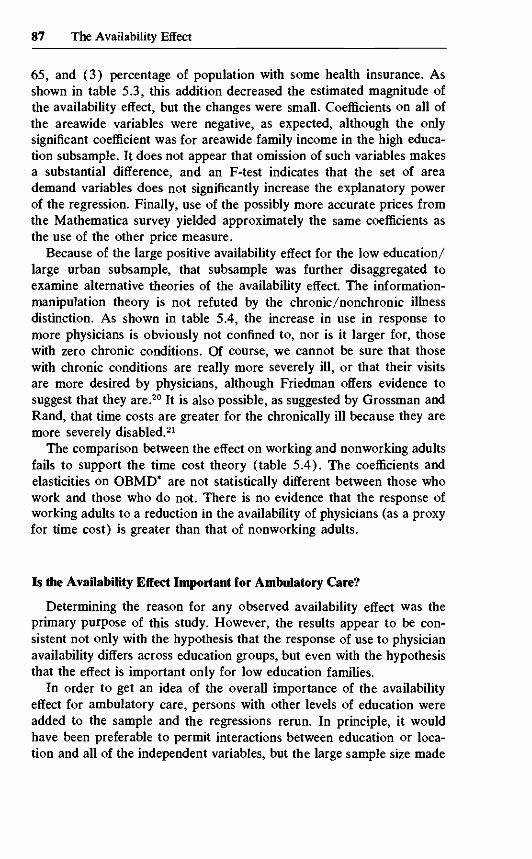
Because a large availability effect was detected for the large urbansubsample, additional analysis was performed on it. First, variablesmeasured in money were deflated by a cost-of-living index, with littlechange in results (table 5.3). Absence of such deflators for the othertwo area subsamples is therefore unlikely to affect results. Next, area-wide demand variables were added to the regressions. The variablesadded were (1) income per capita, (2) percentage of population over

Table 5.3


RAD

CONDS

AGELT15

AGE 45-64

AGE 65 +

Physician Visit Regressions Using Deflated Money Variables,Area Demand Variables, and22 Largest SMSAs,

Money VariablesDeflated by

Cost-of-living Index

Low Head High HeadEducation Education


.257 .407(6.32) (7.21)2.36 2.15

(17.7) (13.1)-.159 -.163

(-0.39) (-0.37).807 -.007

(2.09) (-0.02)2.11 1.41

(4.33) (2.14)

Alternative Price Measures:Persons with Some Visits

Money Variables De-flated and Area De-

mand Variables Added

Low HeadEducation

High HeadEducation

Mathematica FeeEstimates Used

Low HeadEducation

(t statistics in parentheses)

.253(6.13)2.39

(17.6)-.343

(-0.82).787

(2.01)2.05

(4.13)

.412(7.20)2.18

(13.1)-.069

(-0.16).065

(0.15)1.53

(2.26)

.256(6.29)2.36

(17.7)-.163

(-0.40).816

(2.11)2.12

(4.35)

High HeadEducation

.407(7.20)2.15

(13.1)-.174

(-0.40)-.011

(-0.02)1.39

(2.11)

86 Chapter Five



SEX

F15-44

FAMSZ

WORKING

NOINS

FAMINC

GP/MD

SURG/MD

POPDENS

MDFEE

HOSCOST

BEDS*

HBMD*

OBMD*

Inc. Per Cap.

% over 65

% withinsurance(in state)Constant

£2n*

Money VariablesDeflated by

Cost-of-living Index

Low HeadEducation

High HeadEducation


.593(2.15)

.671(1.46)-.100

(-1.14)-.848

(-3.02).028

(0.09).002

(0.70)7.30

(1.63)3.20

(0.34).009

(0.50)-.040

(-0.20)-.024

(-1.46)-1.60

(-0.56)10.9(1.23)34.6(3.18)

-1.00(-0.17)

.1733461

.259(0.80)

.889(1.84)-.090

(-1.17)-1.30

(-3.43)-1.05

(-2.32)-.004

(-2.17)-8.99

(-2.16)-19.6(-0.78)

-.006(-0.31)

.171(0.78)

.028(1.49)

.638(0.24)

— 14.9(-1.65)-26.0(-2.13)

11.1(2.13)

.1462189

Money Variables De-flated and Area De-

mand Variables Added

Low HeadEducation

High HeadEducation

Mathematica FeeEstimates Used

Low HeadEducation

(t statistics in parentheses)

.659(2.35)

.607(1.32)-.080

(-1.11)-.964

(-3.39).037

(0.12).001

(0.49)7.89

(1.43)-1.22

(-0.08).054

(1.61)-.118

(-0.49)-.056

(-2.24)-1.69

(-0.43)8.80

(0.80)28.6(2.08)

-.001(-1.02)

-.163(-0.75)

-.067(-1.69)

14.4(1.06)

.1773311

.272(0.82)

.873(1.78)-.079

(-1.00)-1.17

(-3.49)-1.04

(-2.23)-.005

(-2.37)-14.3(-2.74)-33.4(-2.36)

-.063(-1.60)

.445(1.65)

.034(1.40)1.79

(0.50)-18.2(-1.56)-29.2(-2.23)

-.001(-0.84)

-.256(-1.07)

.044(1.03)16.6(1.23)

.1472126

.592(2.14)

.672(1.47)-.098

(-1-37)-.857

(-3.06).014

(0.05).002

(0.20)5.98

(1.38)-1.87

(-0.18)-.002

(-0.10).154

(0.54)-.030

(-1.83)-.215

(-0.06)16.7(1.65)30.5(2.51)

-.334(-0.17)

.1733461

High HeadEducation

.263(0.80)

.880(1.82)-.087

(-1.13)-1.30

(-3.98)-1.03

(-2.29)-.004

(-2.21)-8.30

(-1.95)-17.8(-1.79)

-.002(-0.10)

.103(0.34)

.019(1.20)-.241

(-0.08)-15.4(-1.46)-25.5(-1.96)

11.8(2.13)

.1462189

* Because of the absence of data for some areas in which the SMS A crosses stateboundaries, the sample size is slightly reduced for the regressions with area de-mand variables.


65, and (3) percentage of population with some health insurance. Asshown in table 5.3, this addition decreased the estimated magnitude ofthe availability effect, but the changes were small. Coefficients on all ofthe areawide variables were negative, as expected, although the onlysignificant coefficient was for areawide family income in the high educa-tion subs ample. It does not appear that omission of such variables makesa substantial difference, and an F-test indicates that the set of areademand variables does not significantly increase the explanatory powerof the regression. Finally, use of the possibly more accurate prices fromthe Mathematica survey yielded approximately the same coefficients asthe use of the other price measure.

Because of the large positive availability effect for the low education/large urban subsample, that subsample was further disaggregated toexamine alternative theories of the availability effect. The information-manipulation theory is not refuted by the chronic/nonchronic illnessdistinction. As shown in table 5.4, the increase in use in response tomore physicians is obviously not confined to, nor is it larger for, thosewith zero chronic conditions. Of course, we cannot be sure that thosewith chronic conditions are really more severely ill, or that their visitsare more desired by physicians, although Friedman offers evidence tosuggest that they are.20 It is also possible, as suggested by Grossman andRand, that time costs are greater for the chronically ill because they aremore severely disabled.21

The comparison between the effect on working and nonworking adultsfails to support the time cost theory (table 5.4). The coefficients andelasticities on OBMD* are not statistically different between those whowork and those who do not. There is no evidence that the response ofworking adults to a reduction in the availability of physicians (as a proxyfor time cost) is greater than that of nonworking adults.

Is the Availability Effect Important for Ambulatory Care?

Determining the reason for any observed availability effect was theprimary purpose of this study. However, the results appear to be con-sistent not only with the hypothesis that the response of use to physicianavailability differs across education groups, but even with the hypothesisthat the effect is important only for low education families.

In order to get an idea of the overall importance of the availabilityeffect for ambulatory care, persons with other levels of education wereadded to the sample and the regressions rerun. In principle, it wouldhave been preferable to permit interactions between education or loca-tion and all of the independent variables, but the large sample size made

88 Chapter Five

Table 5.4 Physician VisitsHouseholds with

Regressions, Persons with Some Visits ini Low Head Education: 22 Largest SMSAs,

Selected Subsamples

Regression Coefficients {t statistics in parentheses)

StatisticVJ Lev H o 1.1 V*

IndependentVariable or

RAD

CONDS

A f i F I T K

AGE 45-64

AGE 65 +

SEX

F 15-44

FAMSZ

VV v^ JX.JV11N VJ

NOINS

FAMINC

GP/MD

SURG/MD

POPDENS

MDFEE

HOSCOST

BEDS*

HBMD*

OBMD*

Constant

nVisits Per Capita

Number of Chronic Conditions

Zero ChronicConditions

.143(2.34)

(1.18).801

(2.07)2.62

(4.91).243

(0.85)1.44

(3.17)- .064(0.82)

1 «-3

(0.52)-.429

(-1.39)— .00002(1.07)

-4 .41(-0.86)-12.40(-1.17)

.016(0.93)-.329(1.36)

.007(0.47)

.775(0.26)

-13.78(-1.49)

21.48(1.92)7.31

(0.21).041

20963.67

Some ChronicConditions

.415(4.12)9 JO

(6.03)1 Ci(\

(0.64)2.05

(1.52)3.33

(2.10).587

(0.65)1.89

(1.18).059

(0.20)1 ClRft

(-1.20)-1.94(1.76)

.00023(2.70)

-2.61(-0.15)-10.51(-0.30)

.018(0.97)

-1.35(-1.54)

-.105(-2.22)-19.45(-2.11)

31.09(1.01)91.89(2.53)21.33(1.67)

.08813658.97

Employment Status

WorkingAdults

.393(2.75)2 51

(7.36)

.546(0.73)3.32

(2.53).581

(0.77)1.48

(1.39)-.053

(-0.08)

.360(0.44)

.0001(1.81)

-3.21(-0.26)

8.23(-0.33)

.014(0.81)

-1.05(-1.62)

-.057(-1.62)-16.29(-2.37)-9.66

(-0.43)43.83(1.68)15.20(1.42)

.2691359

5.00

NonworkingAdults

.301(4.08)3.16

(11.26)

1.71(1.42)2.37

(1-95)1.176

(1.46).821

(0.66).195

(0.87)

-.869(-1.06)

-.00001(-0.17)-3.21

(-0.24)-29.11(-1.07)

.019(1-14)-.889

(-1.38)-.006

(-0.18)-2 .95

(-0.41)24.31(1.05)52.82(1.82)13.00(1.30)

.1871171

7.55


Table 5.5

IndependentStatisticVariable or

RAD

CONDS

AGELT15

AGE 45-64

AGE 65 +

SEX

F 15-44

FAMSZ

WORKING

NOINS

FAMINC

GP/MD

SURG/MD

POPDENS

MDFEE

HOSCOST

BEDS*

HBMD*

OBMD*

MIDED

LOED

SMMET

Physician Visits Regressions, Aggregated Samples:Some Physician Visits

(OLS)


22 LargestSMSAs

.196(7.36)1.58

(24.9).505

(2.64).704

(3.75)1.05

(3.89).068

(0.49)1.29

(6.17)-.163

(-5.73)-.601

(-4.36).269

(1.45).0006

(0.63).164

(0.15)-4.05

(-1.82)-.033

(-2.37).101

(2.90)-.004

(-0.86)-1.37

(-2.25)-.540

(-0.19).700

(0.22)-.027

(-0.20).088

(0.57)

Other SMSAs

.219(8.95)2.01

(30.4)-.033

(-0.16).786

(4.01)1.73

(6.18).172

(1.16)1.35

(6.00)-.089

(-2.69)-.724

(-4.92)-.166

(-0.87)-.002

(-2.17)-2.74

(-1.19)— 14.13(-2.08)

.013(1.50)-.051

(-0.67)-.004

(-0.63)-2.66

(-2.31)-3.20

(-0.71).293

(0.05).010

(0.06).263

(1.47)

Nonmetro-politan Areas

.274(11.1)

1.47(24.1)-.057

(-0.29).737

(2.89)1.03

(3.89)-.004

(-0.03)1.10

(5.14)-.125

(-3.93)-.763

(-5.49)-.096

(-0.59)-.0003

(-0.26).301

(0.49)-1.50

(-1.39).100

(2.60)-.019

(-0.50).016

(3.17).128

(0.39)-.275

(-0.16).981

(1.10).008

(0.05).035

(0.22)

Persons with

All Areas

.231(16.0)

1.70(46.0)

.128(1.11)

.729(6.55)1.30

(8.23).085

(1.07)1.25

(9.94)-.128

(-6.82)-.711

(-8.64).002

(0.02)-.0007

(-1.18)-.049

(-0.09)-2.34

(-2.41).0005

(0.11).063

(2.63).007

(2.27)-.267

(-0.97)-1.73

(-1.33)1.42

(1.66)-.018

(-0.21).120

(1.27)081

( 0.20)

90 Chapter Five


IndependentStatisticVariable or

RURAL

Constant

£2n


22 Largest Nonmetro-SMSAs Other SMSAs politan Areas

4.68(3.36)

.1139736

10.39(3.53)

.14711194

2.79(3.65)

.1299427

All Areas

.112(-0.67)

3.11(4.92)

.13130357

such a procedure prohibitively costly. Dummy variables for educationof head and/or location were included in the regressions.

As indicated in table 5.5, physician stock has a positive but statisti-cally insignificant effect in each of the three location subsamples evenwhen all education groups are combined. When data are combined forall variables and all education levels, one does find that the coefficienton OBMD* is positive and significant at the 90% level. Even here thecoefficient is numerically quite small. With such a large sample, statis-tical significance is usually to be expected. Moreover, the F-tests de-scribed above suggest that it is not proper to combine the subsamplesand constrain coefficients to be equal across subsamples. Accordingly,it seems appropriate to conclude that a positive availability effect forpersons with positive physician visits is difficult to detect, quite small inmagnitude if it is found, and may be due only to specification error.22

For ambulatory visits, then, there appears to be little or no availabil-ity effect when other variables (including health measures) are properlycontrolled. It seems safe to conclude that, for the general population,the availability effect in ambulatory care can safely be ignored.

Documents

The Availability Effect: Empirical · PDF filechapter will develop and use an empirical technique to test for the ... blends or combines normative and positive ... As a result, the