Embed Size (px)
Citation preview

The Basics plus Plotting in X-Y Space

Goal – make scientific illustrations (“generic” of GMT is generic to geo sciences)
Goal – make scientific illustrations
Maps
- Color/bw/shaded topography and bathymetry,
- Point data (earthquakes, seismic or gps stations, etc.),
- Line data (faults, eq rupture zones, roads), - Vector fields w/ error ellipses,
- Focal mechanisms - 3D surface
- Cross sections - Profiles
- Other stuff

What is GMT
GMT is an open source collection of ~60 tools (and and additional 35 support tools) for manipulating geographic and Cartesian
data sets
(including filtering, trend fitting, gridding, projecting, etc.)

What is GMT
Produces PostScript File (PS).
Make illustrations ranging from simple x-y plots to contour maps to artificially
illuminated surfaces and 3-D perspective views

GMT supports ~30 map projections and transformations and comes with support
data such as GSHHS coastlines, rivers, and political boundaries.
If it does not have a map projection you want: it is open source and UNIX.
(i.e. you can do it yourself)

Design Philosophy
Follows the design philosophy of UNIX – filters (linear, single data stream):
data → processing → final illustration.
Processing flow is broken down to a series of elementary steps.
Each step is accomplished by a separate GMT or UNIX tool (machine shop philosophy).

Design Philosophy
Benefits (UNIX only has benefits):
(1) only a few programs are needed (in the world where 60+35 is a “few”, maybe they are referring to the log of the
number of programs.)
(2) each program is small and easy to update and maintain
(maybe – alternate is each task is subroutine that is small and easy to maintain)

Design Philosophy
Benefits (UNIX only has benefits):
(3) each step is independent of the previous step and the data type and can therefore
be used in a variety of applications
(4) the programs can be chained together in shell scripts or with pipes, thereby
creating a process tailored to do a user-specific task

Design Philosophy
GMT was deliberately written for command line usage, not a windows (or interactive) environment, in order to maximize power
and flexibility (i.e. it is hard to use).

Written by Paul Wessel and Walter Smith while graduate students at Lamont Doherty/Columbia University in the mid 80’s when the SUN workstations came out (and UNIX took
over the world). .
(Now at the University of Hawaii and NOAA respectively
The GMT homepage is: gmt.soest.hawaii.edu

GMT documentation
Tutorial
Technical Reference and Cookbook
(aka Manual)
both available on web
http://gmt.soest.hawaii.edu/
in HTML, PDF, and PostScript format.

As is standard with UNIX
GMT is well documented with (UNIX style) “man” pages (also on web).
Entering GMT program/filter name all by itself, or errors in the command
specification (switches, not data) that cause GMT to fall over – dumps the man page to
standard error.

What does/can GMT do?
- Filtering 1-D and 2-D data
(simple processing, GMT is NOT a general Number Cruncher)
output is reprocessed data

Plotting 1-D and 2-D data
- points, lines (symbols, fill, geologic symbols on faults, etc.)
- vector fields

2-D images – grayscale and color, illumination
3-D perspective of 2-D images
histograms, rose diagrams
text
focal mechanism beachballs
Data preparation
gridding, resampling, conversion
Contouring
data base: extraction, merge
cross sections
projection/map transformation (map sphere to plane)
output is reprocessed data
Bookkeeping and bunch of other stuff

GMT Processing Output
1-D ASCII Tables — For example, a (x, y) series may be filtered and the filtered values
output.
ASCII output is written to the standard output stream.

GMT Processing Output
2-D binary (netCDF or user-defined) grid files
Programs that grid ASCII (x, y, z) data or operate on existing grid files produce this
type of output.

GMT Output
Reports – Several GMT programs read input files and report statistics and other
information.
Nearly all programs have an optional “verbose” operation, which reports on the
progress of computation.
Such text is written to the standard error stream

GMT Output
The bulk of GMT output goes to
PostScript
The plotting programs all use the PostScript page description language to describe the
output.
These commands are stored as ASCII text (they are a program in the POSTSCRIPT
language).

output is “PostScript” program – generally ascii text, but not too readable.
(GMT files can get amazingly BIG) % Map boundaries % S 1050 1050 1050 0 360 arc S S 1050 1050 1074 0 360 arc S S 24 W S 1050 1050 1062 -135 -90 arc S S 1050 1050 1062 135 180 arc S S 1050 1050 1062 45 90 arc S S 1050 1050 1062 -45 0 arc S S 1050 1050 1062 -90 -90 arcn S S 2 W S [] 0 B % % End of basemap % S [] 0 B %%Trailer %%BoundingBox: 0 0 647 647 % Reset translations and scale and call showpage S -295 -295 T 4.16667 4.16667 scale 0 A showpage

GMT Output
If you are really ambitious, you can directly edit this file using vi…but in general, don’t.

GMT Output
Postscript is translated by postscript capable (usually laser) printers.
(it is an extra feature one has to buy).

GMT Output
Postscript is also the native language of
- Adobe Illustrator/Photoshop
- ghostscript,
- ghostview.
GMT Output
I frequently use Illustrator to edit GMT produces Postscript prior to using the
figures in papers, presentations, or posters

Apart from the built-in support for coastlines, GMT completely decouples data retrieval/management from the main GMT
programs.
(puts the onus on user! UNIX philosophy)
GMT uses architecture-independent file formats
(flat files – least common denominator).

Effective use of GMT is really effective application of the UNIX philosophy.

Installation/Maintenance - done for us
(by Mitch – THANKS.
Somewhat complicated, not for average user.)
Setup – basic setup done for us
(don’t have to define GMTHOME, path, etc. if use standard CERI .login and .cshrc files)

Installation/Maintenance.
Some common data sets
(GTOPO-30, ETOPO-5, Predicted bathy, etc.)
are installed
“.gmtdefaults” (generic, is .gmtdefaults4 for version 4) file in your home or working directory.
(if you’ve copied something from the tutorial or gotten a script from someone else and it comes out “funny”, the “default” settings may be the culprit).

Easiest way to get started
1) Find system with GMT already set up
2) Get working program (shell script) from someone else and modify (hack) it.
Lots examples in
- Tutorial
- available on www
- available from your “friends”
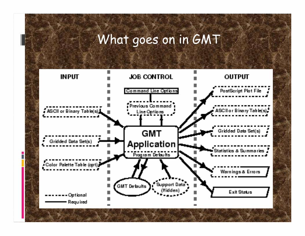
What goes on in GMT

Sources of operational parameters/job control
i) command line options/switches or program defaults
ii) carried over from execution of previous commands
iii) from your .gmtdefaults file (first in working directory if exists, if ~exist, then in your home directory if
exists, finally, system/program defaults)
Sources of operational parameters/job control
Why a defaults file?
- too many parameters to require setting all explicitly (powerful)
- customize – can have different defaults in different directories

Basic GMT use
Most GMT programs read input from terminal (stdin) or files, and write output to
terminal (stdout) (a few write to files).
To write output to files one can use UNIX redirection:
GMTprogram switches >> Outputfile
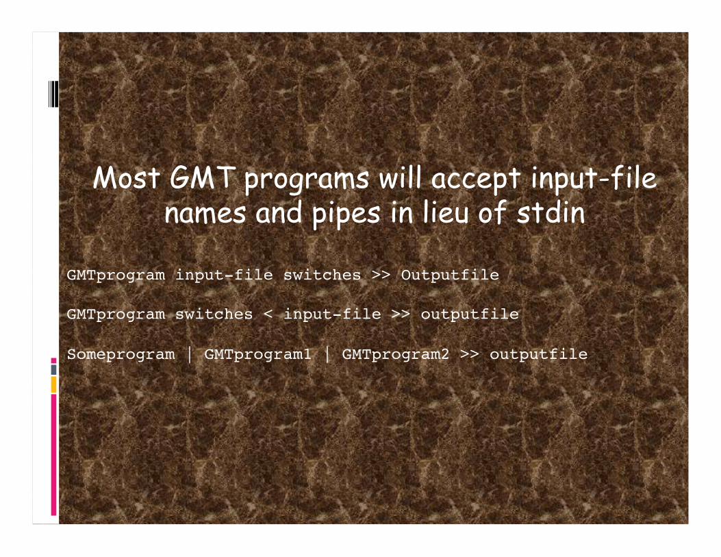
Most GMT programs will accept input-file names and pipes in lieu of stdin
GMTprogram input-file switches >> Outputfile
GMTprogram switches < input-file >> outputfile
Someprogram | GMTprogram1 | GMTprogram2 >> outputfile
Many GMT programs will also accept input redirection (in-line input) – reads whatever follows -- up to character string XXX -- as
input.
GMTprogram switches << END >> output-file .1 .1 .2 .2 END

Can also do with “commnad substitution”:
GMTprogram switches << FIN >> output-file `someprogram swithches < input-file…` FIN
Some GMT programs require input-file names
(usually when need more than one input file)

GMT and scripts
GMT commands, once installed, act much like regular Unix commands.
Generally, the commands are enacted within a shell script so that they may be combined
with other unix commands such as awk.
bash and csh are the most commonly encountered in academia and passing down GMT scripts is how much seismology gets
illustrated

Use Comments!
Comments are very popular to ignore but if you don’t comment your script, 2 years later you may not remember what you were doing.
The spaces and blank lines make your script readable. While it may take more paper if
you print it, it only takes two bytes to make new line or a space.
Keeping track of your scripts
You will be glad (someday) if you set up directories and subdirectories to keep your
maps, data, and scripts organized.
Mitch suggests have something like this in ~/GMT
csh/ data/ ps/ scratch/ sh/
There is a directory for csh scripts, for sh scripts, for data files, for postscript files,
and for scratch files.

OK lets look at some “simple” examples:

Plot x1/2 from 0 to 100 as a dashed line, with red triangles with green borders at x=n*10.

OK lets look at some examples:
1) We start by making the basemap frame for a linear x-y plot.
2) We want it to go from 0 to 100 in x, annotating every 10, and from 0 to 10 in y,
annotating every 2.

3) The final plot should be 4 by 3 inches in size.
Note GMT does not make any helpful assumptions such as
a) You want to plot the whole x and y range of the data and
b) You want it to fit nicely on the page You have to specify EVERYTHNG (comes
under the excuse of being “powerful”)

Here's how we do it: psbasemap -R0/100/0/10 -JX4i/3i -B10/1:."My first plot": -P \ >! plot.ps
We will first look at how the requirements above are specified to make the map.
This is done using the command line options/switches.

Requirements 1 and 3 are specified to GMT together
1) We start by making the basemap frame for a linear x-y plot.
3) The final plot should be 4 by 3 inches in size.

psbasemap draws a map frame and sets up the map parameters (so they don’t have to be re-specified in later GMT program calls)
The –J option selects the type of projection
In this case we want a linear x-y plot, or no projection, which is specified by
x or X.

There are 25 projections available in GMT, each specified by one letter.
There are no provisions for providing your own projection.
(short of using the open source to roll your own.)

Requirements 1 and 3 are specified to GMT together
The –J option also sets the axis scales (distance per unit, x) or (axis length, X)
Where the “unit” is specified in .gmtdefaults or explicitly – inches, i, or cm, c.
psbasemap -R0/100/0/10 -JX4i/3i -B10/1:."My first plot": -P \ >! plot.ps

2) We want it to go from 0 to 100 in x, annotating every 10, and from 0 to 10 in y,
annotating every 1.
This is really two conditions
i) We want it to go from 0 to 100 in x, and from 0 to 10 in y.
Specified by the REGION (-R) option, which (in the usual form) is
-Rxmin/xmax/ymin/ymax

2) We want it to go from 0 to 100 -Rxmin/xmax/ymin/ymax
Notice that unlike MATLAB, GMT does not make any assumptions about what you want
(such as the reasonable one that you just might want the region to show all the
input data).
You have to specify every detail. (i.e. powerful)
(why should the writers of gmt work hard when they can convince the user that
it is “better” if the users do!)
psbasemap -R10/70/-3/8 -JX4i/3i -B10/1:."My first plot": -P \ >! plot.ps

There are two forms for the –R option
1) For projections where the boundaries follow lines of latitude and longitude
(“rectangle” on sphere) – specify sides.
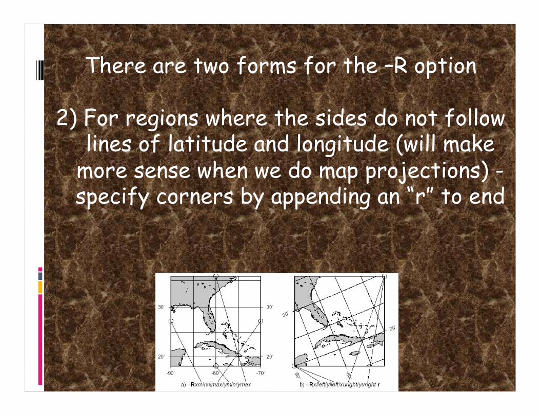
There are two forms for the –R option
2) For regions where the sides do not follow lines of latitude and longitude (will make
more sense when we do map projections) - specify corners by appending an “r” to end
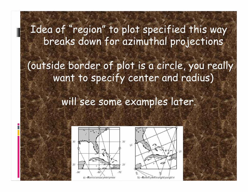
Idea of “region” to plot specified this way breaks down for azimuthal projections
(outside border of plot is a circle, you really want to specify center and radius)
will see some examples later.

2) We want to annotate x every 10, and y every 1.
This is specified by the –B option (Border?).
This is the most complicated GMT option.

Annotation – every 10 for x (first one) and every 1 for y (second one). If you wanted the same annotation for x and y you would
not have to do it twice
psbasemap -R0/100/0/10 -JX4i/3i -B10/1:."My first plot": -P \ >! plot.ps

Not in specs, but controlled by the –B option, the plot title.
This is a little more complicated.
Labels are between colons, with
“.” for plot title, nothing for x axis label,
“,’\” for y axis label.
If label/title is more than one word, has to be in double quotes.
psbasemap -R0/100/0/10 -JX4i/3i -B10/1:."My first plot": -P \ >! plot.ps

If this sounds confusing you can look at the man page for psbasemap for the full
explanation and more examples.
The man page for the –B option, however, is practically incomprehensible.
The BUGS section of the man page states
“The -B option is somewhat complicated to explain and comprehend. However, it is fairly simple for most applications (see
examples). “

Remaining options/switches
-P
Sets the output to Portrait (long side vertical) mode.
“Default” is Landscape (long side horizontal) mode.
psbasemap -R10/70/-3/8 -JX4i/3i -B10/1:."My first plot": -P \ >! plot.ps
This option actually switches “states”.

Remaining options/switches
If .gmtdefaults defines portrait mode as the default, then –P will send it to landscape.
(make a figure and see how it comes out, if you don’t like the orientation stick in a –P).

So, what did we get for all our effort?
Good start – but usually we make plots to show some sort of data
– so how do we do that?

Now let’s look at a more complicated example:
Lets call it “full_court_press.sh” #!/bin/sh #plot square root x sample1d -I1 << END | nawk '{print $1, sqrt($1)}' > {$0}_1.dat 0 100 END psxy -R0/100/0/10 -JX4/2 -Ba20g10/a2f1g2WSne -W5t15_15:0 \ -Y2 -P {$0}_1.dat -K > $0.ps sample1d {$0}_1.dat -I10 | psxy -R -JX4/2 -St0.2 \ -G255/0/0 -W5/0/255/0 -O >> $0.ps

#!/bin/sh #plot square root x sample1d -I1 << END | nawk '{print $1, sqrt($1)}' > {$0}_1.dat 0 100 END psxy -R0/100/0/10 -JX4/2 -Ba20g10/a2f1g2WSne -W5t15_15:0 \ -Y2 -P {$0}_1.dat -K > $0.ps sample1d {$0}_1.dat -I10 | psxy -R -JX4/2 -St0.2 \ -G255/0/0 -W5/0/255/0 -O >> $0.ps
This is a little more than “a little more” complicated.

#!/bin/sh #plot square root x sample1d -I1 << END | nawk '{print $1, sqrt($1)}' > {$0}_1.dat 0 100 END psxy -R0/100/0/10 -JX4/2 -Ba20g10/a2f1g2WSne -W5t15_15:0 \ -Y2 -P {$0}_1.dat -K > $0.ps sample1d {$0}_1.dat -I10 | psxy -R -JX4/2 -St0.2 \ -G255/0/0 -W5/0/255/0 -O >> $0.ps
But it follows the UNIX philosophy – a bunch of simple things stuck together to do
something more complex.
Gives you the idea that most useful GMT produced figures are going to be a LOT of
GMT calls

Here’s what the output looks like (actually the output is a ascii file containing a PostScript program, this is what
it looks like after displaying with GhostScript or printing to a PostScript printer).

Let’s look at it piece, buy simple piece.
Set shell #!/bin/sh #plot square root x sample1d -I1 << END | nawk '{print $1, ...
Set shell to Bourne Shell.
Could also have set it to csh
(change first line to #!/usr/bin/csh -f, this works because this script does not contain anything that is specific to one shell script – such as variable name
definition. Use -f, fast, option which stops it from running your .cshrc).

Next piece
Name the output file. psxy -R0/100/0/10 -JX4/2 -Ba20g10/a2f1g2WSne -W5t15_15:0 \ -Y2 -P {$0}_1.dat -K > $0.ps sample1d {$0}_1.dat -I10 | psxy -R -JX4/2 -St0.2 \ -G255/0/0 -W5/0/255/0 -O >> $0.ps
Being lazy and disorganized - I don’t want to have to type the output file name in lots of times nor keep track of which shell script made which postscript file in my directory.

Next piece
Name the output file. psxy -R0/100/0/10 -JX4/2 -Ba20g10/a2f1g2WSne -W5t15_15:0 \ -Y2 -P {$0}_1.dat -K > $0.ps sample1d {$0}_1.dat -I10 | psxy -R -JX4/2 -St0.2 \ -G255/0/0 -W5/0/255/0 -O >> $0.ps
So I want to find a short and easy way to name the file and I might want to associate the output file name with the name of the
shell script that made it.
Enter UNIX argument passing to the rescue.
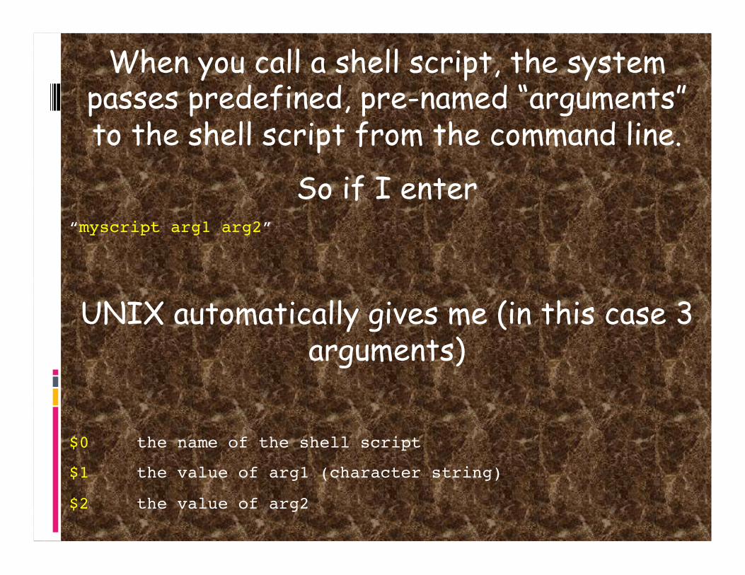
When you call a shell script, the system passes predefined, pre-named “arguments” to the shell script from the command line.
So if I enter “myscript arg1 arg2”
UNIX automatically gives me (in this case 3 arguments)
$0 the name of the shell script
$1 the value of arg1 (character string)
$2 the value of arg2

All I have to do to use these arguments in my shell script (within some constraints) is
stick them in.
The Shell will expand them to their proper values.
So my output file will be named
“full_court_press.sh.ps”,
since $0 will get expanded to “full_court_press.sh”
(the name of the shell script)

Next piece.
Get (actually make) input data – part 1 #!/bin/sh #plot square root x sample1d -I1 << END | nawk '{print $1, sqrt($1)}' > {$0}_1.dat 0 100 END psxy -R0/100/0/10 -JX4/2 -Ba20g10/a2f1g2WSne -W5t15_15:0 \ -Y2 -P {$0}_1.dat -K > $0.ps sample1d {$0}_1.dat -I10 | psxy -R -JX4/2 -St0.2 \ -G255/0/0 -W5/0/255/0 -O >> $0.ps
sample1d, resamples the input - which in this case is redirected (<<) to being obtained in-
line from this file (from end of the command line – which is somewhat far away – to END).

#!/bin/sh sample1d -I1 << END | nawk '{print $1, sqrt($1)}' > {$0}_1.dat 0 100 END psxy -R0/100/0/10 -JX4/2 -Ba20g10/a2f1g2WSne -W5t15_15:0 \ -Y2 -P {$0}_1.dat -K > $0.ps sample1d {$0}_1.dat -I10 | psxy -R -JX4/2 -St0.2 \ -G255/0/0 -W5/0/255/0 -O >> $0.ps
We have to specify the resampling step ( -I1, which is steps of 1).
We will leave everything else at the default values. (see man page if you want more info)
sample1d provides to standard out a list of numbers from 0 to 100 in steps of 1.
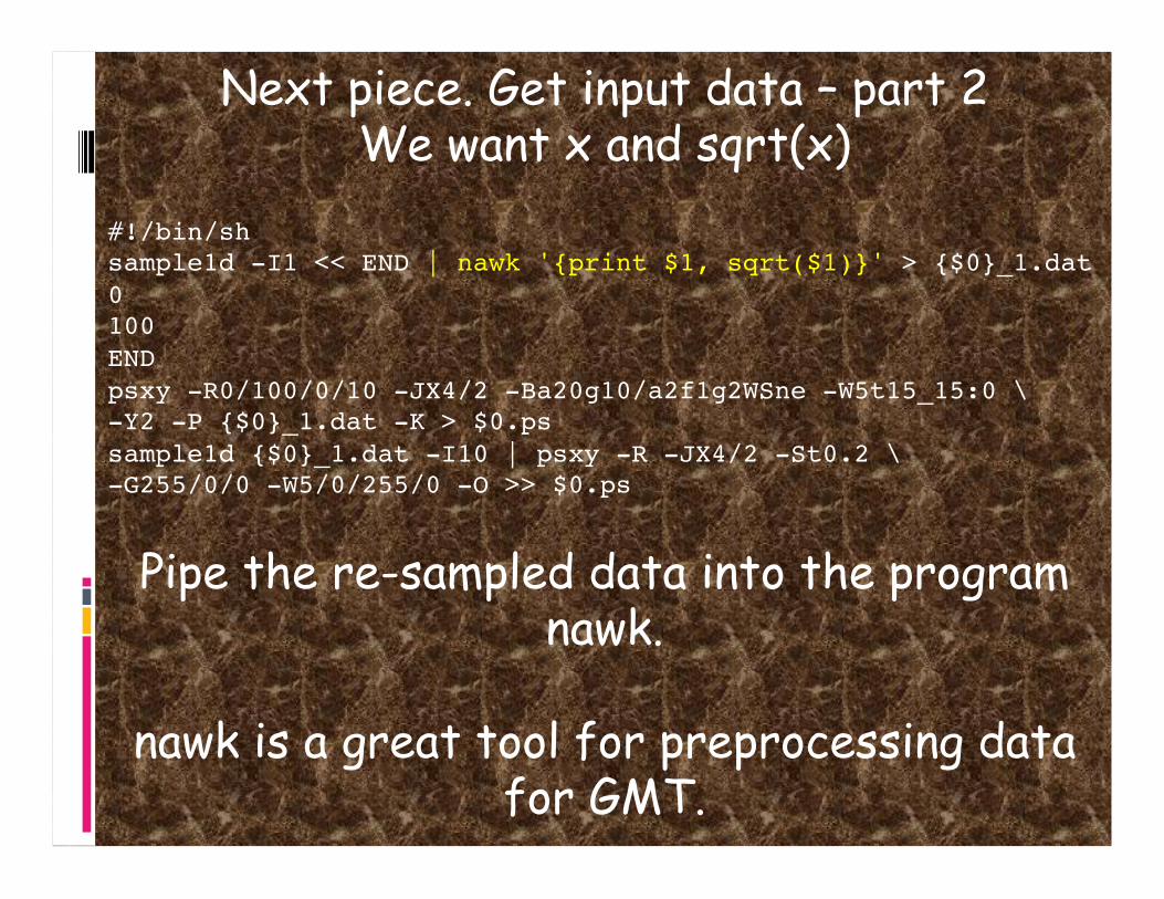
Next piece. Get input data – part 2 We want x and sqrt(x)
#!/bin/sh sample1d -I1 << END | nawk '{print $1, sqrt($1)}' > {$0}_1.dat 0 100 END psxy -R0/100/0/10 -JX4/2 -Ba20g10/a2f1g2WSne -W5t15_15:0 \ -Y2 -P {$0}_1.dat -K > $0.ps sample1d {$0}_1.dat -I10 | psxy -R -JX4/2 -St0.2 \ -G255/0/0 -W5/0/255/0 -O >> $0.ps
Pipe the re-sampled data into the program nawk.
nawk is a great tool for preprocessing data for GMT.

Next piece. Generate input data – part 2
Using nawk, one does not have to write programs to make intermediate files in GMT input format, but can go right to the source data file, read it, modify each line into GMT input format and pipe this directly into the
GMT program. sample1d -I1 << END | nawk '{print $1, sqrt($1)}' | psxy -R0/100/0/10 \ -JX4/2 -Ba20f10g10/a2f1g2WSne -W5t15_15:0 -Y2 -P -K > $0.ps 0 0 100 0 END

Next piece. Generate input data – part 2
sample1d -I1 << END | nawk '{print $1, sqrt($1)}' | psxy -R0/100/0/10 \ -JX4/2 -Ba20f10g10/a2f1g2WSne -W5t15_15:0 -Y2 -P -K > $0.ps 0 0 100 0 END
The nawk command says to print the first column ($1) and the square root of the first
column (sqrt($1)) of every line.
We will (break the UNIX philosophy and) make an intermediate file as we will need it
more than once.

Next piece.
Plot it #!/bin/sh #plot square root x sample1d -I1 << END | nawk '{print $1, sqrt($1)}' > {$0}_1.dat 0 100 END psxy -R0/100/0/10 -JX4/2 -Ba20g10/a2f1g2WSne -W5t15_15:0 \ -Y2 -P {$0}_1.dat -K > $0.ps sample1d {$0}_1.dat -I10 | psxy -R -JX4/2 -St0.2 \ -G255/0/0 -W5/0/255/0 -O >> $0.ps
Finally we get to GMT
psxy is the GMT program that plots points and lines.

#!/bin/sh #plot square root x sample1d -I1 << END | nawk '{print $1, sqrt($1)}' > {$0}_1.dat 0 100 END psxy -R0/100/0/10 -JX4/2 -Ba20g10/a2f1g2WSne -W5t15_15:0 \ -Y2 -P {$0}_1.dat -K > $0.ps sample1d {$0}_1.dat -I10 | psxy -R -JX4/2 -St0.2 \ -G255/0/0 -W5/0/255/0 -O >> $0.ps
psxy accepts the “standard”/”global” options of the GMT filters that produce PostScript
output.
We already know what –R, -J, –B and –P do, although the –B option here is a bit more
complicated looking.

#!/bin/sh #plot square root x sample1d -I1 << END | nawk '{print $1, sqrt($1)}' > {$0}_1.dat 0 100 END psxy -R0/100/0/10 -JX4/2 -Ba20g10/a2f1g2WSne -W5t15_15:0 \ -Y2 -P {$0}_1.dat -K > $0.ps sample1d {$0}_1.dat -I10 | psxy -R -JX4/2 -St0.2 \ -G255/0/0 -W5/0/255/0 -O >> $0.ps
Output file $0.ps (new - is first instance, append in second – this takes care of UNIX
part)
Use \ to continue command on next line

Next piece.
... psxy -R0/100/0/10 -JX4/2 -Ba20g10/a2f1g2WSne -W5t15_15:0 \ -Y2 -P {$0}_1.dat -K > $0.ps ...
So, what’s all that extra stuff on the –B? Each of the letters controls a different
feature/aspect of the plotting of the axis

... psxy -R0/100/0/10 -JX4/2 -Ba20g10/a2f1g2WSne -W5t15_15:0 \ -Y2 -P {$0}_1.dat -K > $0.ps ...
a is for annotation spacing
f is for frame (famous map frame of black/white bars – turned off for x/X, ticks)
g is for grid spacing
WSne says to plot the annotation and ticks on the West and South sides and ticks only
on the north and east sides. (how would you put annotation without ticks?)

Next piece.
Draw a line -W5t15_15:0 ... psxy -R0/100/0/10 -JX4/2 -Ba20g10/a2f1g2WSne -W5t15_15:0 \ -Y2 -P {$0}_1.dat -K > $0.ps . . .

Make line 5 units thick (where units depends on the device and default settings)
-W5t15_15:0

Can also specify color -W5/0t15_15:0 for black line or
-W5/255/0/0t15_15:0 for red line ... psxy -R0/100/0/10 -JX4/2 -Ba20g10/a2f1g2WSne -W5t15_15:0 \ -Y2 -P {$0}_1.dat -K > $0.ps . . .

Make it dashed with dashes 15 units long followed by 15 unit long open spaces -
W5t15_15:0, and a “phase offset” for the dashes of zero -W5t15_15:0

compare to -W5t120_15:60
(line segment 120 long, 15 blank, first line segment 60 long [phase])

This format also works
W[width],[color],[texture]
-W5,0,15_15:-
Gives the same plot.

Next piece. Misc. 1 #!/bin/sh #plot square root x sample1d -I1 << END | nawk '{print $1, sqrt($1)}' > {$0}_1.dat 0 100 END psxy -R0/100/0/10 -JX4/2 -Ba20g10/a2f1g2WSne -W5t15_15:0 \ -Y2 -P {$0}_1.dat -K > $0.ps sample1d {$0}_1.dat -I10 | psxy -R -JX4/2 -St0.2 \ -G255/0/0 -W5/0/255/0 -O >> $0.ps
-Y2 offset plot 2 units in the Y direction (else x axis labels get cut off across bottom of plot)
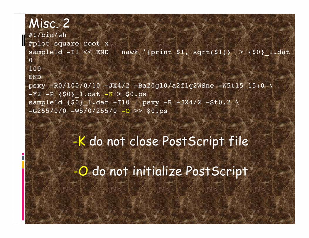
Misc. 2 #!/bin/sh #plot square root x sample1d -I1 << END | nawk '{print $1, sqrt($1)}' > {$0}_1.dat 0 100 END psxy -R0/100/0/10 -JX4/2 -Ba20g10/a2f1g2WSne -W5t15_15:0 \ -Y2 -P {$0}_1.dat -K > $0.ps sample1d {$0}_1.dat -I10 | psxy -R -JX4/2 -St0.2 \ -G255/0/0 -W5/0/255/0 -O >> $0.ps
-K do not close PostScript file
-O do not initialize PostScript

-K do not close PostScript file (don’t
output “showpage”) so more PostScript can be
appended to the file
-O do not initialize PostScript
(does not output PostScript header
stuff) so this can be appended to existing file (that hopefully
does not have a showpage at the end).

Misc. 3
Several common “gotchas”
– no showpage (can see on screen, but does not print – actually prints a blank page) (have
a –K in last GMT call)
- showpage in middle of file (forgot the –K somewhere) – only get part of file on screen
or in final print or get ghostscript error message.
- Have header in middle of file (forgot –O somewhere), get ghostscript error message.
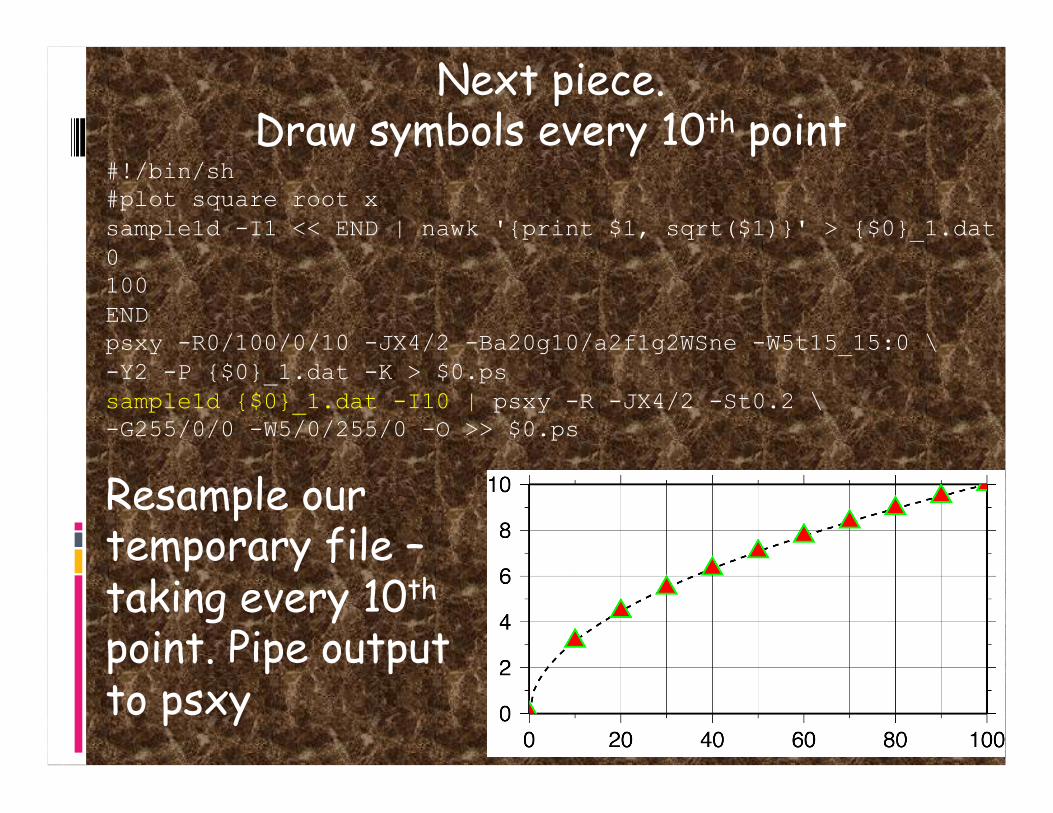
Next piece. Draw symbols every 10th point
#!/bin/sh #plot square root x sample1d -I1 << END | nawk '{print $1, sqrt($1)}' > {$0}_1.dat 0 100 END psxy -R0/100/0/10 -JX4/2 -Ba20g10/a2f1g2WSne -W5t15_15:0 \ -Y2 -P {$0}_1.dat -K > $0.ps sample1d {$0}_1.dat -I10 | psxy -R -JX4/2 -St0.2 \ -G255/0/0 -W5/0/255/0 -O >> $0.ps
Resample our temporary file – taking every 10th point. Pipe output to psxy
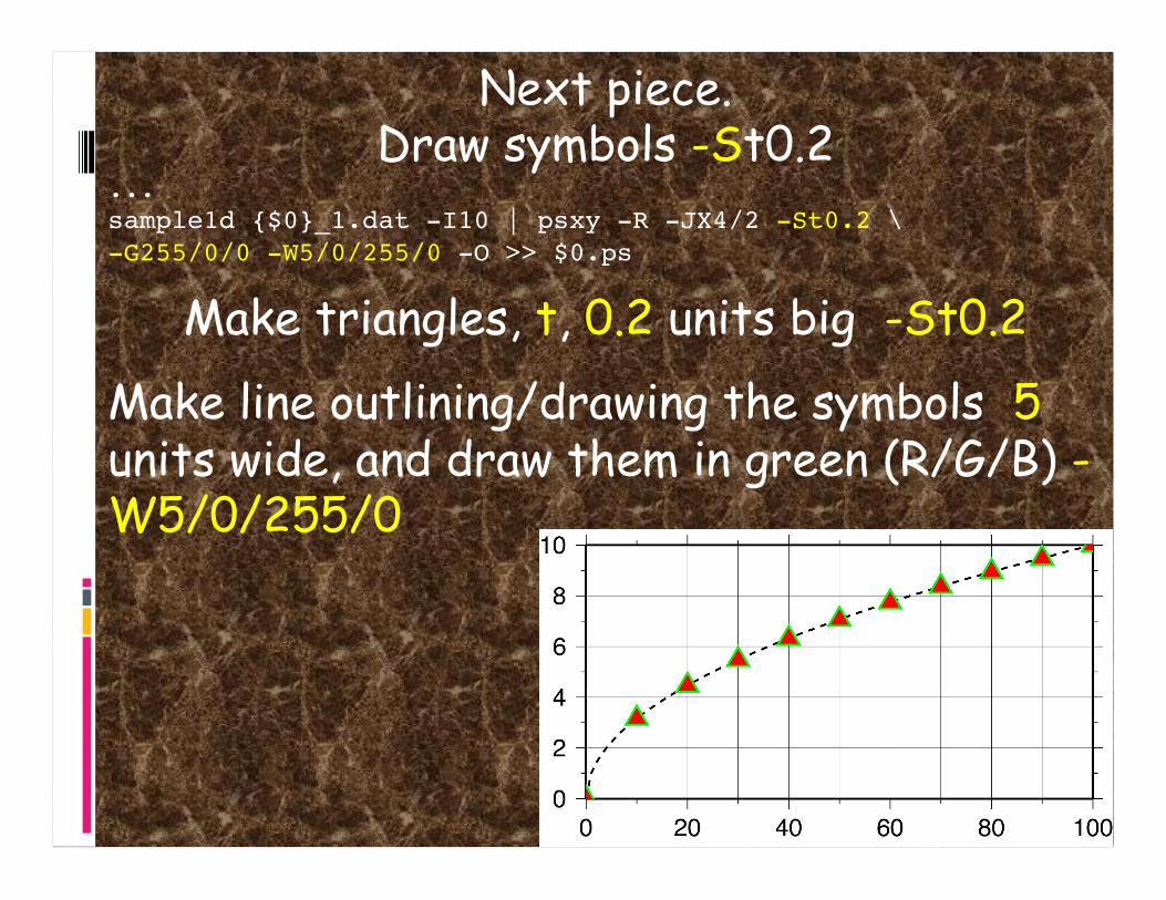
Next piece. Draw symbols -St0.2
... sample1d {$0}_1.dat -I10 | psxy -R -JX4/2 -St0.2 \ -G255/0/0 -W5/0/255/0 -O >> $0.ps
Make triangles, t, 0.2 units big -St0.2
Make line outlining/drawing the symbols 5 units wide, and draw them in green (R/G/B) -W5/0/255/0

Fill symbols color red (R/G/B) -G255/0/0
Colors specified in R/G/B format (intensity of Red, Green and Blue color guns – primary colors for additive
system).
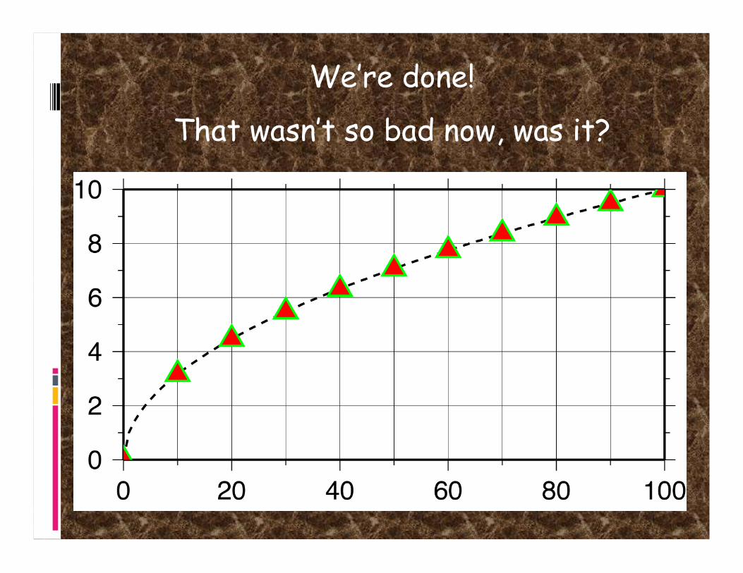
We’re done!
That wasn’t so bad now, was it?

There are two other non-map-projected forms
1) Logarithmic - add l (lower case letter L) after scale of axis you want logarithmic -
JX4l/2

2) Power/exponential – add p and exponent after scale of axis you want exponential (can
scale axes individually)
-JX4p0.5/2

Common command options on first, and possibly subsequent, calls
Need on all calls
-R Define region for plot – will need on first call and at least “–R” on subsequent
-J define projection for plot – will need this on all calls if need to define region
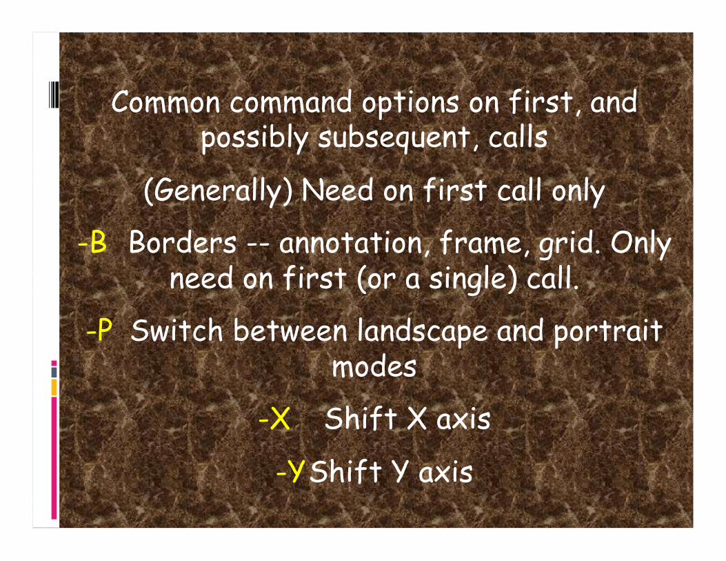
Common command options on first, and possibly subsequent, calls
(Generally) Need on first call only
-B Borders -- annotation, frame, grid. Only need on first (or a single) call.
-P Switch between landscape and portrait modes
-X Shift X axis
-Y Shift Y axis

Common command options on first, and possibly subsequent, calls.
Need when needed.
-K Don’t close PostScript (showpage), use when more will follow
- need on all but last GMT call
-O Don’t initialize PostScript, use when appending to pre-existing file
- need on all but first GMT call
- use both –K and –O when putting a large number of GMT call outputs together

Common command options on first, and possibly subsequent, calls.
Need when needed.
-V Verbose (prints out stuff to standard error for user).
-H Header records (tells GMT to skip first H lines of ascii input file)

How about making
pretty
MAPS?
(this was made by the shell script I put in Mitch’s GMT -ToT web page.)
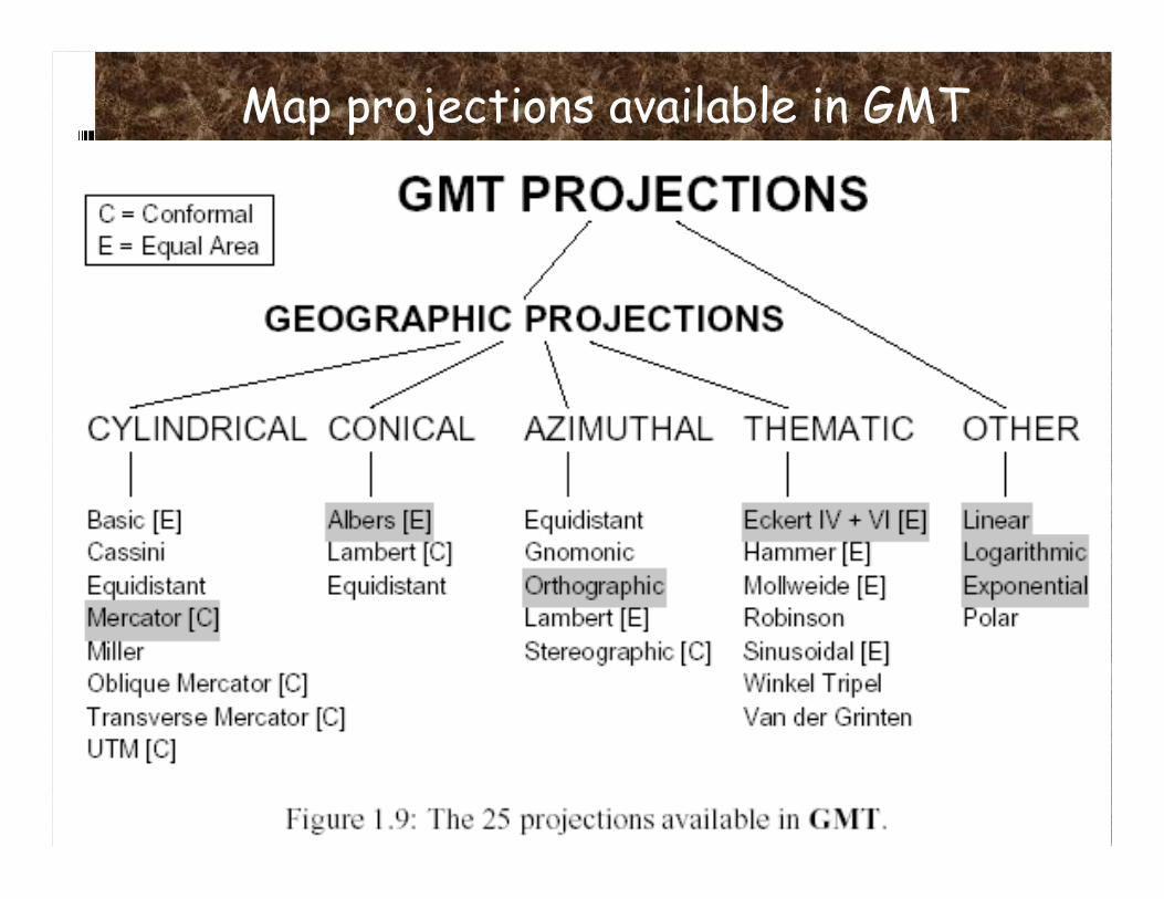
Map projections available in GMT

List of “standard” command line
options.
The –J option sets the “projection”
One has to look at the man page for
each one as “different things
vary” We will now look at the
examples from the tutorial
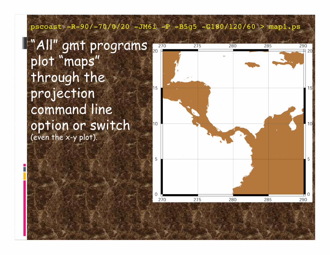
pscoast -R-90/-70/0/20 -JM6i -P -B5g5 -G180/120/60 > map1.ps
“All” gmt programs plot “maps” through the projection command line option or switch (even the x-y plot).

pscoast -R-90/-70/0/20 -JM6i -P -B5g5 -G180/120/60 > map1.ps
All projections give you two selections for specifying the scale
(note GMT takes the mapmakers attitude that a map has to have a predetermined/known scale – nicely filling the page does not cut it.)

pscoast -R-90/-70/0/20 -JM6i -P -B5g5 -G180/120/60 > map1.ps
-Jmparameters
(Mercator [C]).
Specify one of: -Jmscale or -JMwidth
Give scale along equator (1:xxxx or UNIT/degree).

pscoast -R-90/-70/0/20 -JM6i -P -B5g5 -G180/120/60 > map1.ps
-Jmlon0/lat0/scale or
-JMlon0/lat0/width
Give central meridian, standard latitude and scale along parallel (1:xxxx or UNIT/degree, UNIT = number inches or cms).

Mercator Projection:
One way to address plotting sphere on a plane (which is whole ‘nother subject)
Conformal (maintains shapes)
Cylindrical projection
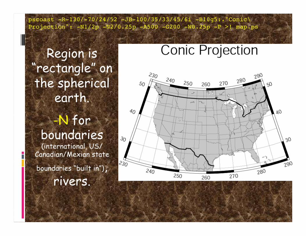
pscoast -R-130/-70/24/52 -JB-100/35/33/45/6i -B10g5:."Conic\ Projection": -N1/2p -N2/0.25p -A500 -G200 -W0.25p -P >! map.ps
Region is “rectangle” on the spherical
earth.
-N for boundaries (international, US/
Canadian/Mexian state
boundaries “built in”), rivers.

pscoast -R-130/-70/24/52 -JB-100/35/33/45/6i -B10g5:."Conic\ Projection": -N1/2p -N2/0.25p -A500 -G200 -W0.25p -P >! map.ps
-A to get rid of small
water/island features
Projection (b/B) – need to
know something
(center and standard parallels).
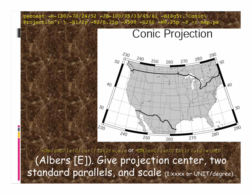
pscoast -R-130/-70/24/52 -JB-100/35/33/45/6i -B10g5:."Conic\ Projection": \ -N1/2p -N2/0.25p -A500 -G200 -W0.25p -P >! map.ps
-Jblon0/lat0/lat1/lat2/scale or -JBlon0/lat0/lat1/lat2/width
(Albers [E]). Give projection center, two standard parallels, and scale (1:xxxx or UNIT/degree).

Albers
Also conformal (maintains/conserves shape)
Conical projection
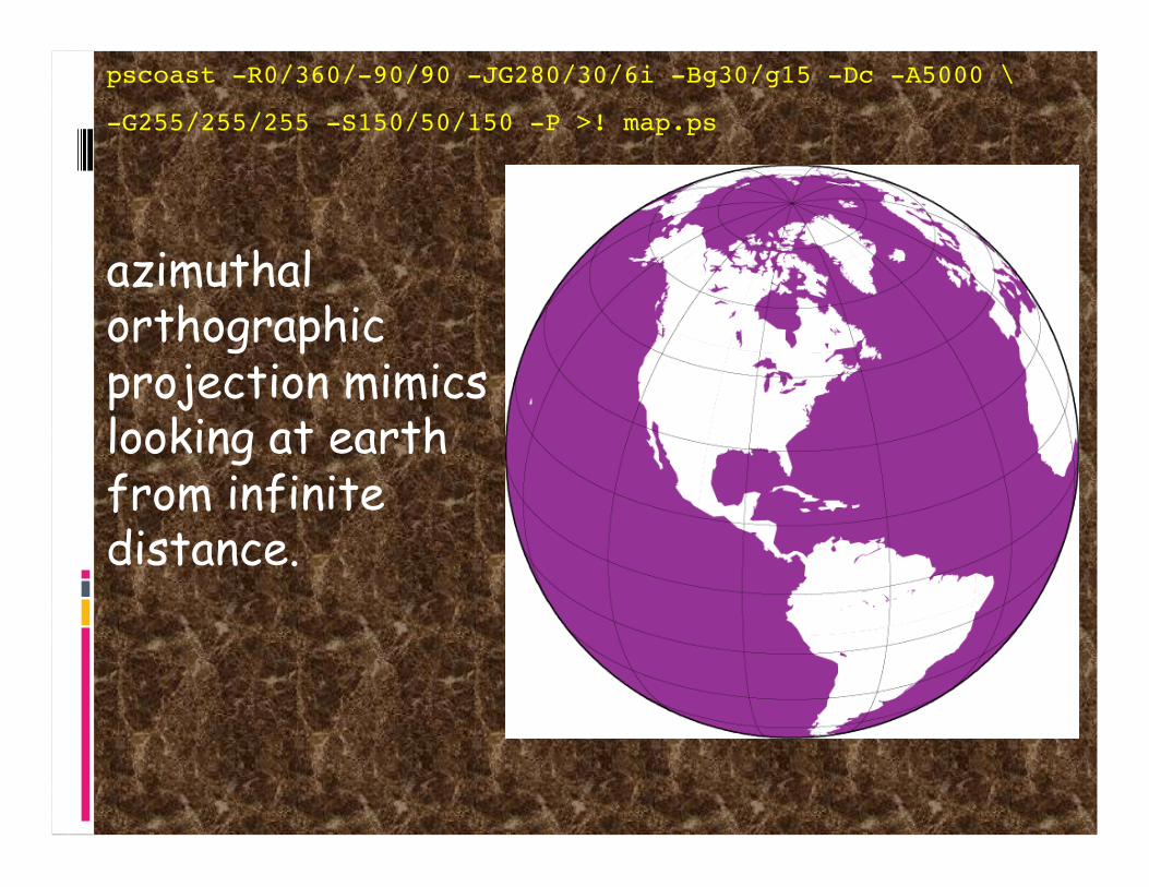
pscoast -R0/360/-90/90 -JG280/30/6i -Bg30/g15 -Dc -A5000 \
-G255/255/255 -S150/50/150 -P >! map.ps
azimuthal orthographic projection mimics looking at earth from infinite distance.

pscoast -R0/360/-90/90 -JG280/30/6i -Bg30/g15 -Dc -A5000 \
-G255/255/255 -S150/50/150 -P >! map.ps
New option
-Dc
Controls resolution of coastline
f full
h high
l low
c crude
Helps manage file

Some useful maps.
The world centered on
Memphis.
Use to get back
azimuth and distance to earthquakes at a glance.

NOTE:
GMT will fall over in this projection if there is land at the anti-pode and you try to fill it. (fill should be donut between coastline and outside of map but PostScript interpreter – which does fill - will do something else).

Part I of shell script
Set stuff up #!/bin/sh #call with “stn_az_map lat lon name” ROOT=/gaia/home/smalley WORLDCOAST=0/360/0/180 RED=250/50/50 BLUE=50/50/255 GREEN=50/255/50 MOREPS=-K ADDPS=-O CONTINUEPS=”-K –O” FILL=200 SCALE=1.75 XOFFSET=0.75 YOFFSET=1.5 GRIDCNTR=180/90/7/90 OUTPUTFILE=$0_$3.ps rm $OUTPUTFILE
Notice abundant “comments” (use variable names that are self documenting)

#set up map to be centered on lat lon given in command line #draw crude coastlines, ocean blue, land green #do not draw lat long grid (no frame specs on –B, could put w/next)pscoast -R$WORLDCOAST -Je$1/$2/$SCALE/180 -B:."Station $3 Map": -S200/200/255 -G200/250/200 -W1 -Dc -P $MOREPS -X$XOFFSET -Y$YOFFSET > $OUTPUTFILE
#set up new map centered on north pole and draw only the lat long grid psbasemap -R$WORLDCOAST -Je$GRIDCNTR -B15g15 -O -K >> $OUTPUTFILE
#RESET map to be centered on lat lon given in command line #to put on some earthquake data read from this file #data specified in lat long order, psxy assumes long lat (x,y) so #use the “-:” switch to let psxy know (another common gotcha) psxy -R$WORLDCOAST -Je$1/$2/$SCALE/180 -Sc0.1 -G250/250/50 -W1/0/0/0 $CONTINUEPS -: <<END >> $OUTPUTFILE-9.09 158.4435.35 78.13END
#add plate boundaries, notice don’t have to respecify details of region and projection but do need –R -Je psxy -R -Je -M$ -W1/$RED $CONTINUEPS $ROOT/ptect/ridges >> $OUTPUTFILEpsxy -R -Je -M$ -W1/$GREEN $CONTINUEPS $ROOT/ptect/xforms >> $OUTPUTFILEpsxy -R -Je -M$ -W1/$BLUE $ADDPS $ROOT/ptect/trenches >> $OUTPUTFILE

Another version of an azimuthal, equiangular
map centered on Memphis and it’s anti-pode.
Now it’s a lot easier to identify landmasses on the other side of the globe by their shapes.
Also shows that great circles (the radial lines)
converge at the anti-pode.
(also solves antipode fill problem)

Nazca-South America Euler pole
Data plotted in South America reference frame using oblique Mercator projection
referenced to Euler pole (points on South America plate have zero – or near zero – velocities.).
Plate motion follows lines of latitude (horizontal lines).
Kendrick et al, 2003

Typical task:
Somebody gives you a file with earthquake data (and if you are lucky a description of the file)
So we have
lat in col 8, lon in col 9, depth in col 10 and magnitude in col 11
ZDEQ 64 1 1 5 14 26.76 37.285 143.002 26.9 4.4 0 15 27.0229 5 1.82 7.21 2.95 200.86 9 0 1 5 DEQ 64 1 1 12 21 58.64 -6.872 129.763 111.1 0.0 0 58 95.0280 7 1.19 6.21 2.69 66.99 17 11 3 27 …

We can use the following nawk command (can put it into shell script) to produce GMT output for psxy – lat long and magnitude for example (psxy can scale the symbols from the data – use magnitude for scaling).
I usually do it on the fly and pipe or suck it into the GMT program. If it’s needed in more than one place – put it in a temporary file.
nawk '{print $9, $8, $11}' EBH.HDF
Produces the following output for GMT 143.002 37.285 4.4 129.763 -6.872 0.0

So what do we do with our nawk command nawk '{print $9, $8, $11}' EBH.HDF
You can put this into GMT several ways
If this is the only file you want to plot – this would work
nawk '{print $9, $8, $11}' EBH.HDF | pxsy …

If you had a number of files that needed conversion you could do it this way (only need
one psxy call)
psxy … << END … … `nawk '{print $9, $8, $11}' EBH.HDF` … END
Converting each file on the fly.
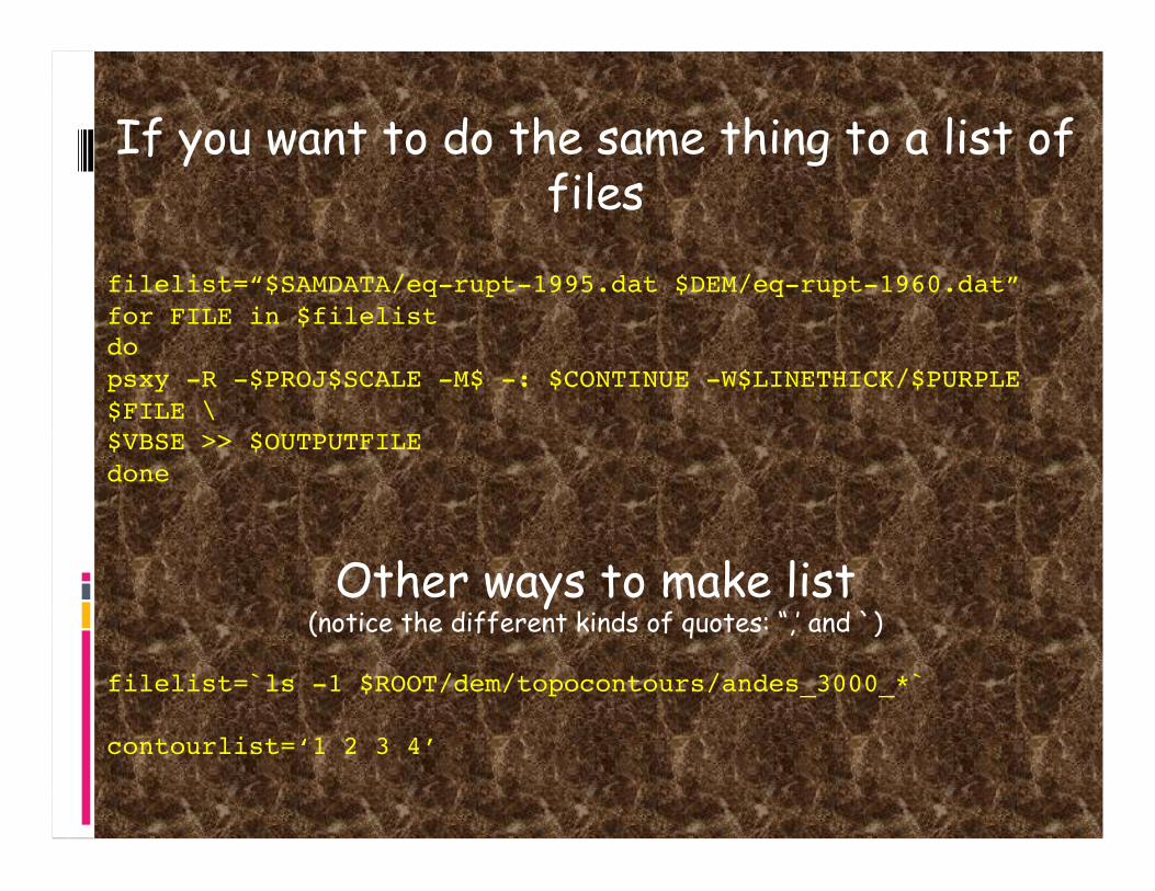
If you want to do the same thing to a list of files
filelist=“$SAMDATA/eq-rupt-1995.dat $DEM/eq-rupt-1960.dat” for FILE in $filelist do psxy -R -$PROJ$SCALE -M$ -: $CONTINUE -W$LINETHICK/$PURPLE $FILE \ $VBSE >> $OUTPUTFILE done
Other ways to make list (notice the different kinds of quotes: “,’ and `)
filelist=`ls -1 $ROOT/dem/topocontours/andes_3000_*`
contourlist=‘1 2 3 4’
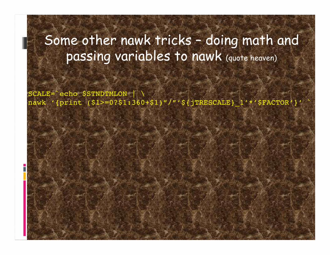
Some other nawk tricks – doing math and passing variables to nawk (quote heaven)
SCALE=`echo $STNDTMLON | \ nawk ‘{print ($1>=0?$1:360+$1)”/”’${jTRESCALE}_1’*’$FACTOR’}’ `