Embed Size (px)
Citation preview

The Basics:
SPSS®
for Windows®
19329-001
SPSS 11.5 10/15/2002 ro/mh/ss
For more information about SPSS® software products, please visit our Web site at http://www.spss.com or contact
SPSS Inc.233 South Wacker Drive, 11th FloorChicago, IL 60606-6412Tel: (312) 651-3000Fax: (312) 651-3668
SPSS is a registered trademark and its other product names are the trademarks of SPSS Inc. for its proprietary computer software. No material describing such software may be produced or distributed without the written permission of the owners of the trademark and license rights in the software and the copyrights in the published materials.
The SOFTWARE and documentation are provided with RESTRICTED RIGHTS. Use, duplication, or disclosure by the Government is subject to restrictions as set forth in subdivision (c)(1)(ii) of The Rights in Technical Data and Computer Software clause at 52.227-7013. Contractor/manufacturer is SPSS Inc., 233 South Wacker Drive, 11th Floor, Chicago, IL 60606-6412.
TableLook is a trademark of SPSS Inc.Windows is a registered trademark of Microsoft Corporation.DataDirect, DataDirect Connect, INTERSOLV, and SequeLink are registered trademarks of MERANT Solutions Inc.Portions of this product were created using LEADTOOLS © 1991-2000, LEAD Technologies, Inc. ALL RIGHTS RESERVED.LEAD, LEADTOOLS, and LEADVIEW are registered trademarks of LEAD Technologies, Inc.Portions of this product were based on the work of the FreeType Team (http:\\www.freetype.org).
General notice: Other product names mentioned herein are used for identification purposes only and may be trademarks or registered trademarks of their respective companies in the United States and other countries.
The Basics: SPSS® for Windows®
Copyright © 2002 by SPSS Inc.All rights reserved.Printed in the United States of America.
No part of this publication may be reproduced, stored in a retrieval system, or transmitted, in any form or by any means, electronic, mechanical, photocopying, recording, or otherwise, without the prior written permission of the publisher.
3
C o n t e n t s
1 Introduction 9
Introduction . . . . . . . . . . . . . . . . . . . . . . . . . . . . . . . . . . . . . . . . . . 9
Sample Files . . . . . . . . . . . . . . . . . . . . . . . . . . . . . . . . . . . . . . . . . . 9
Starting SPSS . . . . . . . . . . . . . . . . . . . . . . . . . . . . . . . . . . . . . . . . . 10
Note about Data File Access When Running SPSS from a Remote Server . . . . 10
Variable Display in Dialog Boxes . . . . . . . . . . . . . . . . . . . . . . . . . . . . 11
Opening a Data File . . . . . . . . . . . . . . . . . . . . . . . . . . . . . . . . . . . . . . 11
Running an Analysis . . . . . . . . . . . . . . . . . . . . . . . . . . . . . . . . . . . . . 14
Viewing Results . . . . . . . . . . . . . . . . . . . . . . . . . . . . . . . . . . . . . . . . 17
Creating Charts . . . . . . . . . . . . . . . . . . . . . . . . . . . . . . . . . . . . . . . . 18
Leaving SPSS . . . . . . . . . . . . . . . . . . . . . . . . . . . . . . . . . . . . . . . . . 19
2 Using the Help System 21
Help Contents Tab . . . . . . . . . . . . . . . . . . . . . . . . . . . . . . . . . . . . . . 22
Index Window . . . . . . . . . . . . . . . . . . . . . . . . . . . . . . . . . . . . . . . . . 23
Dialog Box Help . . . . . . . . . . . . . . . . . . . . . . . . . . . . . . . . . . . . . . . . 24
Right-Mouse Context Help. . . . . . . . . . . . . . . . . . . . . . . . . . . . . . . . . . 25
Statistics Coach. . . . . . . . . . . . . . . . . . . . . . . . . . . . . . . . . . . . . . . . 26
Results Coach . . . . . . . . . . . . . . . . . . . . . . . . . . . . . . . . . . . . . . . . . 32
Case Studies. . . . . . . . . . . . . . . . . . . . . . . . . . . . . . . . . . . . . . . . . . 34
3 Sources and Organization of Data 35
Introduction . . . . . . . . . . . . . . . . . . . . . . . . . . . . . . . . . . . . . . . . . . 35
Sources of Data . . . . . . . . . . . . . . . . . . . . . . . . . . . . . . . . . . . . . . . . 35
Data Organization in SPSS. . . . . . . . . . . . . . . . . . . . . . . . . . . . . . . . . . 36
Rows . . . . . . . . . . . . . . . . . . . . . . . . . . . . . . . . . . . . . . . . . . . . 36
Columns . . . . . . . . . . . . . . . . . . . . . . . . . . . . . . . . . . . . . . . . . . 36
Design a Coding Scheme . . . . . . . . . . . . . . . . . . . . . . . . . . . . . . . . . . 37
Identification Fields . . . . . . . . . . . . . . . . . . . . . . . . . . . . . . . . . . . 37
4
Choices in Entering Data . . . . . . . . . . . . . . . . . . . . . . . . . . . . . . . . . . 38
SPSS Data Entry . . . . . . . . . . . . . . . . . . . . . . . . . . . . . . . . . . . . . 38
Extensions . . . . . . . . . . . . . . . . . . . . . . . . . . . . . . . . . . . . . . . . . . 38
Summary . . . . . . . . . . . . . . . . . . . . . . . . . . . . . . . . . . . . . . . . . . . 38
Appendix: Sample Data from an Engineering Application . . . . . . . . . . . . . . . 39
4 Reading Data 41
Reading Data . . . . . . . . . . . . . . . . . . . . . . . . . . . . . . . . . . . . . . . . . 41
Basic Structure of an SPSS Data File . . . . . . . . . . . . . . . . . . . . . . . . . . . 41
Reading an SPSS Data File . . . . . . . . . . . . . . . . . . . . . . . . . . . . . . . . . 42
Reading Data from Spreadsheets . . . . . . . . . . . . . . . . . . . . . . . . . . . . . 44
Reading Data from a Database. . . . . . . . . . . . . . . . . . . . . . . . . . . . . . . 46
Reading Data from a Text File . . . . . . . . . . . . . . . . . . . . . . . . . . . . . . . 53
Saving Data . . . . . . . . . . . . . . . . . . . . . . . . . . . . . . . . . . . . . . . . . . 60
Appendix: Reading Fixed-Column Text Data . . . . . . . . . . . . . . . . . . . . . . . 62
5 Using the Data Editor 77
Using the Data Editor . . . . . . . . . . . . . . . . . . . . . . . . . . . . . . . . . . . . 77
Entering Numeric Data . . . . . . . . . . . . . . . . . . . . . . . . . . . . . . . . . . . 77
Entering String Data . . . . . . . . . . . . . . . . . . . . . . . . . . . . . . . . . . . . . 80
Defining Data . . . . . . . . . . . . . . . . . . . . . . . . . . . . . . . . . . . . . . . . . 82
Adding a Variable Label. . . . . . . . . . . . . . . . . . . . . . . . . . . . . . . . . 82
Changing Variable Type and Format . . . . . . . . . . . . . . . . . . . . . . . . . 83
Adding Value Labels for Numeric Variables . . . . . . . . . . . . . . . . . . . . . 84
Adding Value Labels for String Variables . . . . . . . . . . . . . . . . . . . . . . . 86
Using Value Labels for Data Entry . . . . . . . . . . . . . . . . . . . . . . . . . . . 88
Handling Missing Data . . . . . . . . . . . . . . . . . . . . . . . . . . . . . . . . . 89
Missing Values for a Numeric Variable . . . . . . . . . . . . . . . . . . . . . . . . 90
Missing Values for a String Variable . . . . . . . . . . . . . . . . . . . . . . . . . 91
Copy and Paste Value Attributes . . . . . . . . . . . . . . . . . . . . . . . . . . . 93
6 Examining Summary Statistics for
Individual Variables 99
Examining Summary Statistics for Individual Variables . . . . . . . . . . . . . . . . . 99
Level of Measurement. . . . . . . . . . . . . . . . . . . . . . . . . . . . . . . . . . . . 99
5
Summary Measures for Categorical Data . . . . . . . . . . . . . . . . . . . . . . . . 100
Charts for Categorical Data . . . . . . . . . . . . . . . . . . . . . . . . . . . . . . 102
Summary Measures for Scale Variables. . . . . . . . . . . . . . . . . . . . . . . . . 103
Histograms for Scale Variables . . . . . . . . . . . . . . . . . . . . . . . . . . . . 105
Assessing Degree of Missing Data with Descriptives . . . . . . . . . . . . . . . . . 106
7 Modifying Data Values 109
Modifying Data Values . . . . . . . . . . . . . . . . . . . . . . . . . . . . . . . . . . . 109
Creating a Categorical Variable from a Scale Variable . . . . . . . . . . . . . . . . 109
Two Simple Recoding Rules. . . . . . . . . . . . . . . . . . . . . . . . . . . . . . 112
Computing New Variables . . . . . . . . . . . . . . . . . . . . . . . . . . . . . . . . . 112
Computing Variables With Missing Values . . . . . . . . . . . . . . . . . . . . . . . 114
8 Crosstabulation Tables 119
Crosstabulation Tables . . . . . . . . . . . . . . . . . . . . . . . . . . . . . . . . . . . 119
Simple Crosstabulation. . . . . . . . . . . . . . . . . . . . . . . . . . . . . . . . . . . 119
Counts versus Percentages . . . . . . . . . . . . . . . . . . . . . . . . . . . . . . . . 121
Significance Testing for Crosstabulations . . . . . . . . . . . . . . . . . . . . . . . . 122
Adding a Layer Variable . . . . . . . . . . . . . . . . . . . . . . . . . . . . . . . . . . 124
9 Working With Output 127
Using the Viewer . . . . . . . . . . . . . . . . . . . . . . . . . . . . . . . . . . . . . . 127
Using the Pivot Table Editor . . . . . . . . . . . . . . . . . . . . . . . . . . . . . . . . 129
Explanations and Definitions of Output . . . . . . . . . . . . . . . . . . . . . . . 129
Pivoting a Table . . . . . . . . . . . . . . . . . . . . . . . . . . . . . . . . . . . . . 130
Creating and Displaying Layers . . . . . . . . . . . . . . . . . . . . . . . . . . . . 132
Editing Tables . . . . . . . . . . . . . . . . . . . . . . . . . . . . . . . . . . . . . . 134
Hiding Rows and Columns . . . . . . . . . . . . . . . . . . . . . . . . . . . . . . . 135
Changing Data Display Formats . . . . . . . . . . . . . . . . . . . . . . . . . . . 136
TableLooks. . . . . . . . . . . . . . . . . . . . . . . . . . . . . . . . . . . . . . . . . . 138
Using Predefined Formats . . . . . . . . . . . . . . . . . . . . . . . . . . . . . . . 138
Customizing TableLook Styles . . . . . . . . . . . . . . . . . . . . . . . . . . . . 139
Changing the Default Table Formatting . . . . . . . . . . . . . . . . . . . . . . . 141
Customizing Initial Display Settings . . . . . . . . . . . . . . . . . . . . . . . . . 143
Optionally Displaying Variable and Value Labels . . . . . . . . . . . . . . . . . . 145
6
Using Results in Other Applications . . . . . . . . . . . . . . . . . . . . . . . . . . . .147
Pasting Results as Rich Text . . . . . . . . . . . . . . . . . . . . . . . . . . . . . .147
Pasting Results as Metafiles . . . . . . . . . . . . . . . . . . . . . . . . . . . . . .149
Pasting Results as Text . . . . . . . . . . . . . . . . . . . . . . . . . . . . . . . . .151
Exporting Output . . . . . . . . . . . . . . . . . . . . . . . . . . . . . . . . . . . . . . .152
10 Creating and Editing Charts 155
Creating and Editing Charts . . . . . . . . . . . . . . . . . . . . . . . . . . . . . . . . .155
Creating a Standard Chart . . . . . . . . . . . . . . . . . . . . . . . . . . . . . . . . .155
Editing Standard Charts . . . . . . . . . . . . . . . . . . . . . . . . . . . . . . . . . . .157
Creating Interactive Charts . . . . . . . . . . . . . . . . . . . . . . . . . . . . . . . . .162
Editing Interactive Ch\arts . . . . . . . . . . . . . . . . . . . . . . . . . . . . . . . . .165
Creating an Interactive Chart from a Pivot Table . . . . . . . . . . . . . . . . . . . .168
11 Time Saving Features 171
SPSS Syntax . . . . . . . . . . . . . . . . . . . . . . . . . . . . . . . . . . . . . . . . .171
Copying Data Properties . . . . . . . . . . . . . . . . . . . . . . . . . . . . . . . . . .174
Displaying Data Dictionary Information . . . . . . . . . . . . . . . . . . . . . . . . . .180
Dialog Recall . . . . . . . . . . . . . . . . . . . . . . . . . . . . . . . . . . . . . . . . .181
SPSS Options . . . . . . . . . . . . . . . . . . . . . . . . . . . . . . . . . . . . . . . . .183
12 Multiple Response Variables 185
Introduction to Multiple Response Variables . . . . . . . . . . . . . . . . . . . . . . .185
What are Multiple Response Variables? . . . . . . . . . . . . . . . . . . . . . . . . .185
Defining a Multiple Response Set . . . . . . . . . . . . . . . . . . . . . . . . . . . . .187
Defining a Multiple Response Set: Dichotomous Items . . . . . . . . . . . . . . . . .190
Multiple Response Frequency Tables . . . . . . . . . . . . . . . . . . . . . . . . . . .192
Crosstab Tables with Multiple Response Variables . . . . . . . . . . . . . . . . . . .194
Handling Nonresponses. . . . . . . . . . . . . . . . . . . . . . . . . . . . . . . . . . .196
Other Procedures and Multiple Response Variables . . . . . . . . . . . . . . . . . .197
Summary . . . . . . . . . . . . . . . . . . . . . . . . . . . . . . . . . . . . . . . . . . .198
7
13 Hands-On Exercises 199
Background for the Bank Data File . . . . . . . . . . . . . . . . . . . . . . . . . . . . 199
Data Location . . . . . . . . . . . . . . . . . . . . . . . . . . . . . . . . . . . . . . . . 199
Using the Help System . . . . . . . . . . . . . . . . . . . . . . . . . . . . . . . . . . . 199
Reading Data . . . . . . . . . . . . . . . . . . . . . . . . . . . . . . . . . . . . . . . . 200
Labels and Missing Values (reference chapter: Using the Data Editor) . . . . . . . 201
Examining Summary Statistics for Individual Variables . . . . . . . . . . . . . . . . 202
Modifying Data Values . . . . . . . . . . . . . . . . . . . . . . . . . . . . . . . . . . . 202
Crosstabulation Tables . . . . . . . . . . . . . . . . . . . . . . . . . . . . . . . . . . . 203
Working with Output . . . . . . . . . . . . . . . . . . . . . . . . . . . . . . . . . . . . 203
Creating and Editing Charts . . . . . . . . . . . . . . . . . . . . . . . . . . . . . . . . 204
Time Saving Features . . . . . . . . . . . . . . . . . . . . . . . . . . . . . . . . . . . 204
Multiple Response Variables . . . . . . . . . . . . . . . . . . . . . . . . . . . . . . . 204
Index 207

9
Chapte r
1Introduction
Introduction
The goal of this course is to enable you to perform useful analyses on your data with SPSS. Keeping this in mind, the following chapters include such topics as reading data, adding labels, performing basic statistical analyses, modifying data, and creating charts. This course guide will focus on the key elements necessary for you to answer basic questions from your data.
This chapter will introduce you to the basic environment of SPSS and demonstrate a typical session. We will run SPSS, retrieve a previously defined SPSS data file, and then produce a simple statistical summary and a chart. In the process you will learn the roles of the primary windows within SPSS and see a few features that smooth the way when running analyses.
More detailed instruction about many of the topics touched upon in this chapter will follow in later chapters. Here, we hope to give you a basic framework for understanding and using SPSS.
Once you are at the Windows desktop, you start SPSS by double-clicking on the short-cut labeled SPSS for Windows (if present), or by using the Start menu.
Sample Files
Most of the examples presented here use the data file demo.sav. This data file is a fictitious survey of several thousand people, containing basic demographic and consumer information.
All sample files used in these examples are located in the tutorial\sample files folder within the folder in which SPSS is installed.
10
Chapter 1
Starting SPSS
To start SPSS:
� From the Start menu choose:
ProgramsSPSS for Windows
SPSS for Windows
or
ProgramsSPSS for Windows Student Version
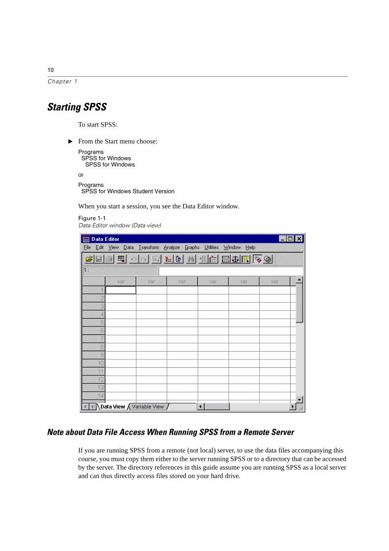
When you start a session, you see the Data Editor window.
Figure 1-1
Data Editor window (Data view)
Note about Data File Access When Running SPSS from a Remote Server
If you are running SPSS from a remote (not local) server, to use the data files accompanying this course, you must copy them either to the server running SPSS or to a directory that can be accessed by the server. The directory references in this guide assume you are running SPSS as a local server and can thus directly access files stored on your hard drive.
11
Introduction
When you start SPSS, a dialog box opens, prompting you to access data or run a tutorial.
� Press Cancel to close this dialog box.
One window (the Data Editor window) is open when you start SPSS. Other SPSS windows will open as we create and edit tables and charts, or create SPSS syntax commands. We will view some of these windows in the course of this chapter; others will be explored later in the course. The toolbars contain useful shortcuts and helpful features when running SPSS.
Variable Display in Dialog Boxes
Either variable names or longer variable labels will appear in list boxes in dialog boxes. Additionally, variables in list boxes can be ordered alphabetically or by their position in the file.
In this course, we will display variable labels in alphabetic order within list boxes. For a new user of SPSS, this provides a more complete description of variables in an easy-to-follow order. In more advanced courses, we typically display variable names in alphabetic order.
Since the default setting within SPSS is to display variable labels in file order, we will change this before accessing data.
� From the menus, choose:
EditOptions
� Click Display labels in the Variable Lists group of the General tab.
� Click Alphabetical.
� Click OK and then click OK to confirm the change.
Opening a Data File
Before you can analyze data, you need some data to analyze.
To open a data file:
� From the menus, choose:
FileOpen
Data
Alternatively, you can use the Open File button on the toolbar.
Figure 1-2
Open File toolbar button
12
Chapter 1
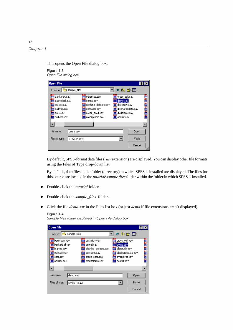
This opens the Open File dialog box.
Figure 1-3
Open File dialog box
By default, SPSS-format data files (.sav extension) are displayed. You can display other file formats using the Files of Type drop-down list.
By default, data files in the folder (directory) in which SPSS is installed are displayed. The files for this course are located in the tutorial\sample files folder within the folder in which SPSS is installed.
� Double-click the tutorial folder.
� Double-click the sample_files folder.
� Click the file demo.sav in the Files list box (or just demo if file extensions aren’t displayed).
Figure 1-4
Sample files folder displayed in Open File dialog box
13
Introduction
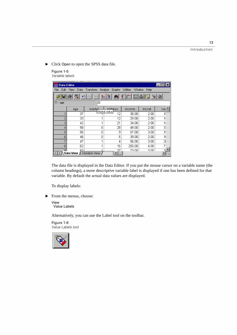
� Click Open to open the SPSS data file.
Figure 1-5
Variable labels
The data file is displayed in the Data Editor. If you put the mouse cursor on a variable name (the column headings), a more descriptive variable label is displayed if one has been defined for that variable. By default the actual data values are displayed.
To display labels:
� From the menus, choose:
ViewValue Labels
Alternatively, you can use the Label tool on the toolbar.
Figure 1-6
Value Labels tool
14
Chapter 1
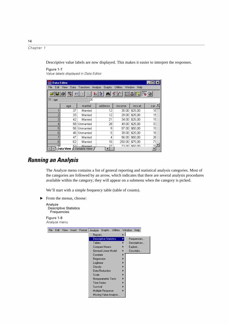
Descriptive value labels are now displayed. This makes it easier to interpret the responses.
Figure 1-7
Value labels displayed in Data Editor
Running an Analysis
The Analyze menu contains a list of general reporting and statistical analysis categories. Most of the categories are followed by an arrow, which indicates that there are several analysis procedures available within the category; they will appear on a submenu when the category is picked.
We’ll start with a simple frequency table (table of counts).
� From the menus, choose:
AnalyzeDescriptive Statistics
Frequencies
Figure 1-8
Analyze menu
15
Introduction
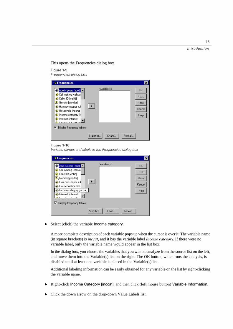
This opens the Frequencies dialog box.
Figure 1-9
Frequencies dialog box
Figure 1-10
Variable names and labels in the Frequencies dialog box
� Select (click) the variable Income category.
A more complete description of each variable pops up when the cursor is over it. The variable name (in square brackets) is inccat, and it has the variable label Income category. If there were no variable label, only the variable name would appear in the list box.
In the dialog box, you choose the variables that you want to analyze from the source list on the left, and move them into the Variable(s) list on the right. The OK button, which runs the analysis, is disabled until at least one variable is placed in the Variable(s) list.
Additional labeling information can be easily obtained for any variable on the list by right-clicking the variable name.
� Right-click Income Category [inccat], and then click (left mouse button) Variable Information.
� Click the down arrow on the drop-down Value Labels list.
16
Chapter 1
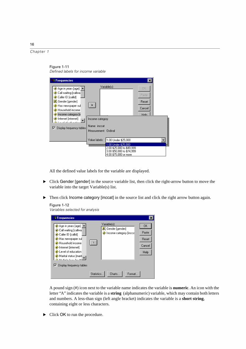
Figure 1-11
Defined labels for income variable
All the defined value labels for the variable are displayed.
� Click Gender [gender] in the source variable list, then click the right-arrow button to move the variable into the target Variable(s) list.
� Then click Income category [inccat] in the source list and click the right arrow button again.
Figure 1-12
Variables selected for analysis
A pound sign (#) icon next to the variable name indicates the variable is numeric. An icon with the letter “A” indicates the variable is a string (alphanumeric) variable, which may contain both letters and numbers. A less-than sign (left angle bracket) indicates the variable is a short string,containing eight or less characters.
� Click OK to run the procedure.
17
Introduction
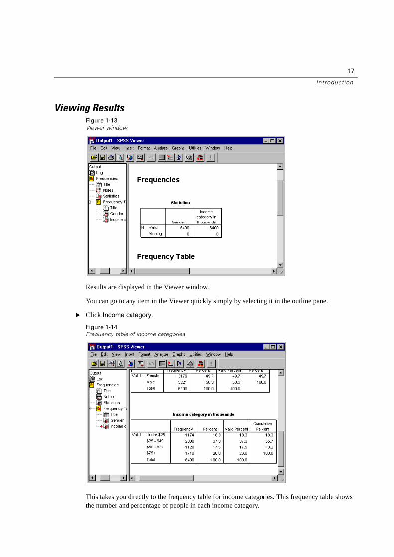
Viewing ResultsFigure 1-13
Viewer window
Results are displayed in the Viewer window.
You can go to any item in the Viewer quickly simply by selecting it in the outline pane.
� Click Income category.
Figure 1-14
Frequency table of income categories
This takes you directly to the frequency table for income categories. This frequency table shows the number and percentage of people in each income category.
18
Chapter 1
Creating Charts
Although some statistical procedures can create high-resolution charts, you can also use the Graphs menu to create charts. For example, you could create a chart that shows the relationship between wireless telephone service and PDA (personal digital assistant) ownership.
� From the menus, choose:
GraphsBar
� Click Clustered and then click OK.
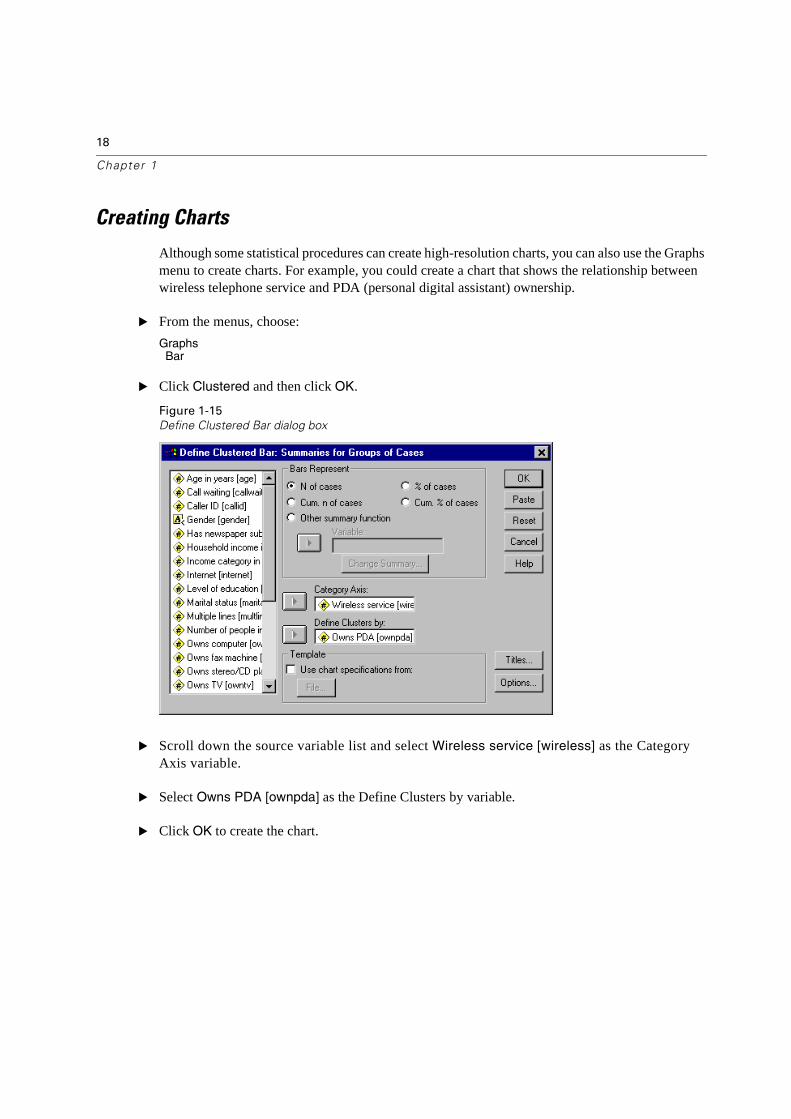
Figure 1-15
Define Clustered Bar dialog box
� Scroll down the source variable list and select Wireless service [wireless] as the CategoryAxis variable.
� Select Owns PDA [ownpda] as the Define Clusters by variable.
� Click OK to create the chart.
19
Introduction
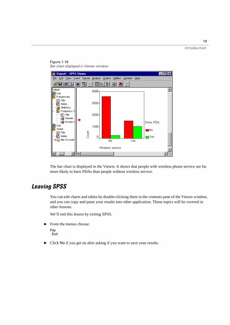
Figure 1-16
Bar chart displayed in Viewer window
The bar chart is displayed in the Viewer. It shows that people with wireless phone service are far more likely to have PDAs than people without wireless service.
Leaving SPSS
You can edit charts and tables by double-clicking them in the contents pane of the Viewer window, and you can copy and paste your results into other application. Those topics will be covered in other lessons.
We’ll end this lesson by exiting SPSS.
� From the menus choose:
FileExit
� Click No if you get an alert asking if you want to save your results.

21
Chapte r
2Using the Help System
Help is available in a number of different ways, including:
Help menu. Every window has a Help menu on the menu bar. The Topics menu item provides access to the help system, where you can use the Contents and Index tabs to find topics. The Tutorial menu item provides access to the introductory tutorial.
Dialog box Help buttons. Most dialog boxes have a Help button that takes you directly to a Help topic for that dialog box. The Help topic provides general information and links to related topics.
Pivot table context menu Help. Right-click on terms in an activated pivot table in the Viewer and select What’s This? from the context menu to display definitions of the terms.
Statistics Coach. The Statistics Coach item on the Help menu provides a wizard-like method for finding the right statistical or charting procedure for what you want to do.
Case Studies. The Case Studies item on the Help menu provides hands-on examples of how to create various types of statistical analyses and interpret the results. The sample data files used in the examples are also provided so you can work through the examples to see exactly how the results were produced.
This chapter uses the files demo.sav and bhelptut.spo.
22
Chapter 2
Help Contents Tab
The Topics item on the help menu opens a help window.
� From the menus choose:
HelpTopics
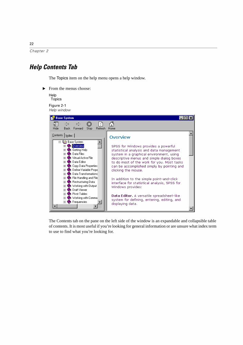
Figure 2-1
Help window
The Contents tab on the pane on the left side of the window is an expandable and collapsible table of contents. It is most useful if you’re looking for general information or are unsure what index term to use to find what you’re looking for.
23
Using the Help System
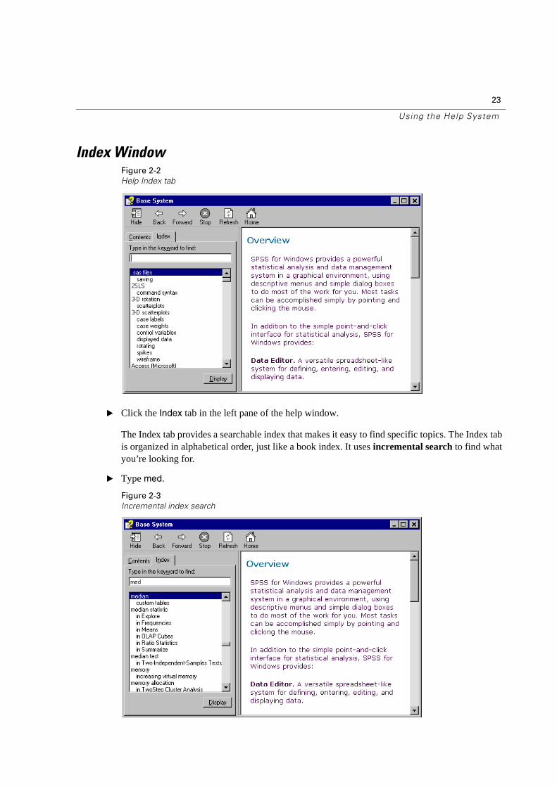
Index WindowFigure 2-2
Help Index tab
� Click the Index tab in the left pane of the help window.
The Index tab provides a searchable index that makes it easy to find specific topics. The Index tab is organized in alphabetical order, just like a book index. It uses incremental search to find what you’re looking for.
� Type med.
Figure 2-3
Incremental index search
24
Chapter 2
The index scrolls to and highlights the first index entry that starts with those letters: median.
Dialog Box Help
Most dialog boxes have a help button that displays a help topic about what the dialog box does and how to do it.
� From the menus, choose:
AnalyzeDescriptive Statistics
Frequencies
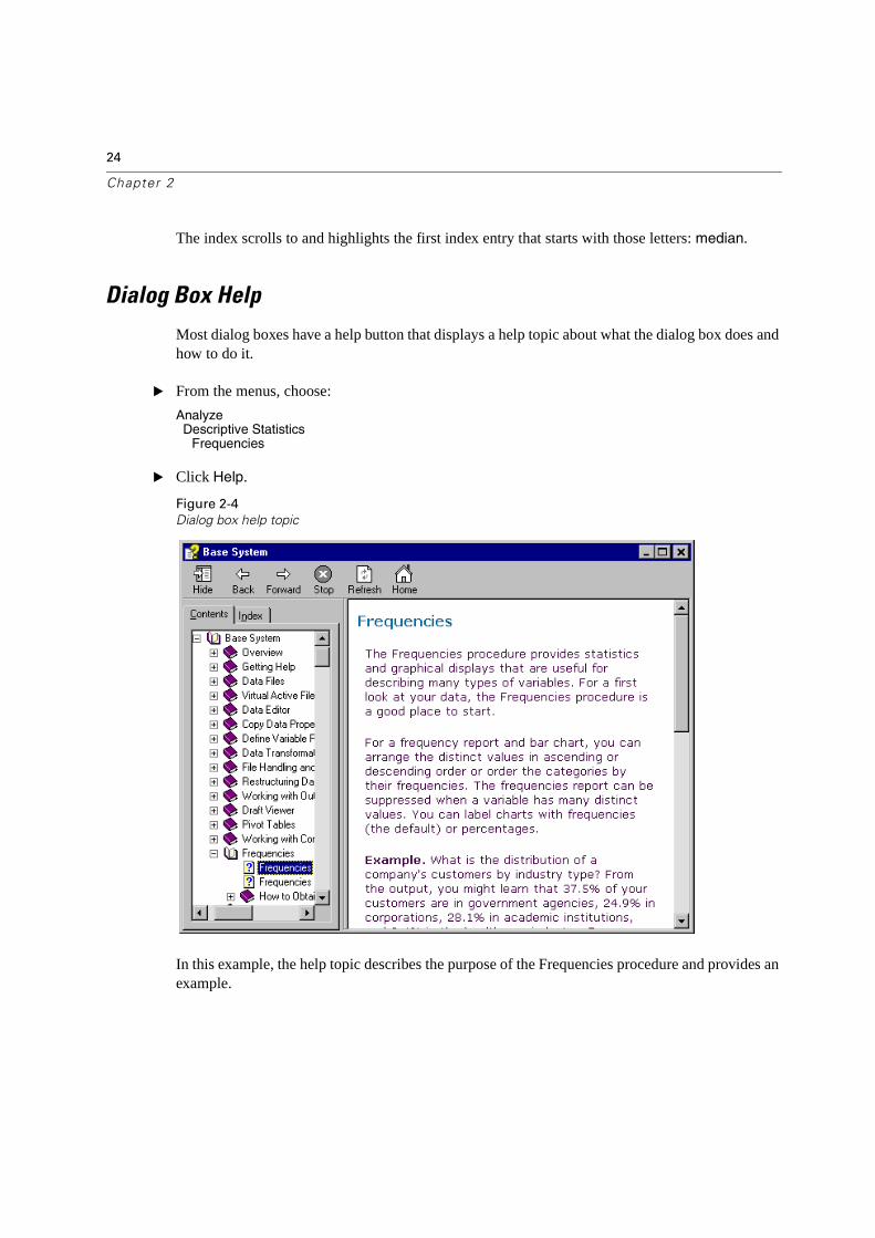
� Click Help.
Figure 2-4
Dialog box help topic
In this example, the help topic describes the purpose of the Frequencies procedure and provides an example.
25
Using the Help System
Right-Mouse Context Help
Context-sensitive help is also available for individual controls and terms that appear in many dialog boxes.
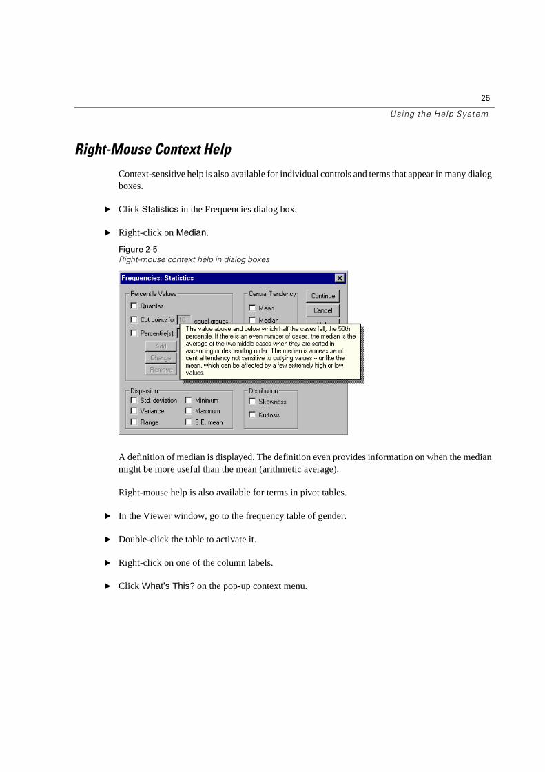
� Click Statistics in the Frequencies dialog box.
� Right-click on Median.
Figure 2-5
Right-mouse context help in dialog boxes
A definition of median is displayed. The definition even provides information on when the median might be more useful than the mean (arithmetic average).
Right-mouse help is also available for terms in pivot tables.
� In the Viewer window, go to the frequency table of gender.
� Double-click the table to activate it.
� Right-click on one of the column labels.
� Click What’s This? on the pop-up context menu.
26
Chapter 2
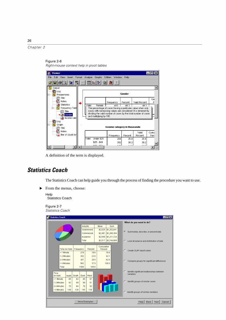
Figure 2-6
Right-mouse context help in pivot tables
A definition of the term is displayed.
Statistics Coach
The Statistics Coach can help guide you through the process of finding the procedure you want to use.
� From the menus, choose:
HelpStatistics Coach
Figure 2-7
Statistics Coach
27
Using the Help System
The Coach presents a series of questions designed to find the appropriate procedure. The first question is simply "What do you want to do?"
For example, if you want to summarize data...
� Click Summarize, describe, or present data.
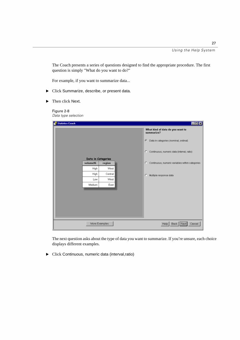
� Then click Next.
Figure 2-8
Data type selection
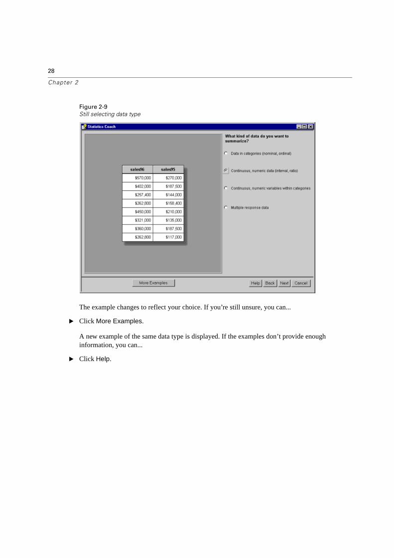
The next question asks about the type of data you want to summarize. If you’re unsure, each choice displays different examples.
� Click Continuous, numeric data (interval,ratio)
28
Chapter 2
Figure 2-9
Still selecting data type
The example changes to reflect your choice. If you’re still unsure, you can...
� Click More Examples.
A new example of the same data type is displayed. If the examples don’t provide enough information, you can...
� Click Help.
29
Using the Help System
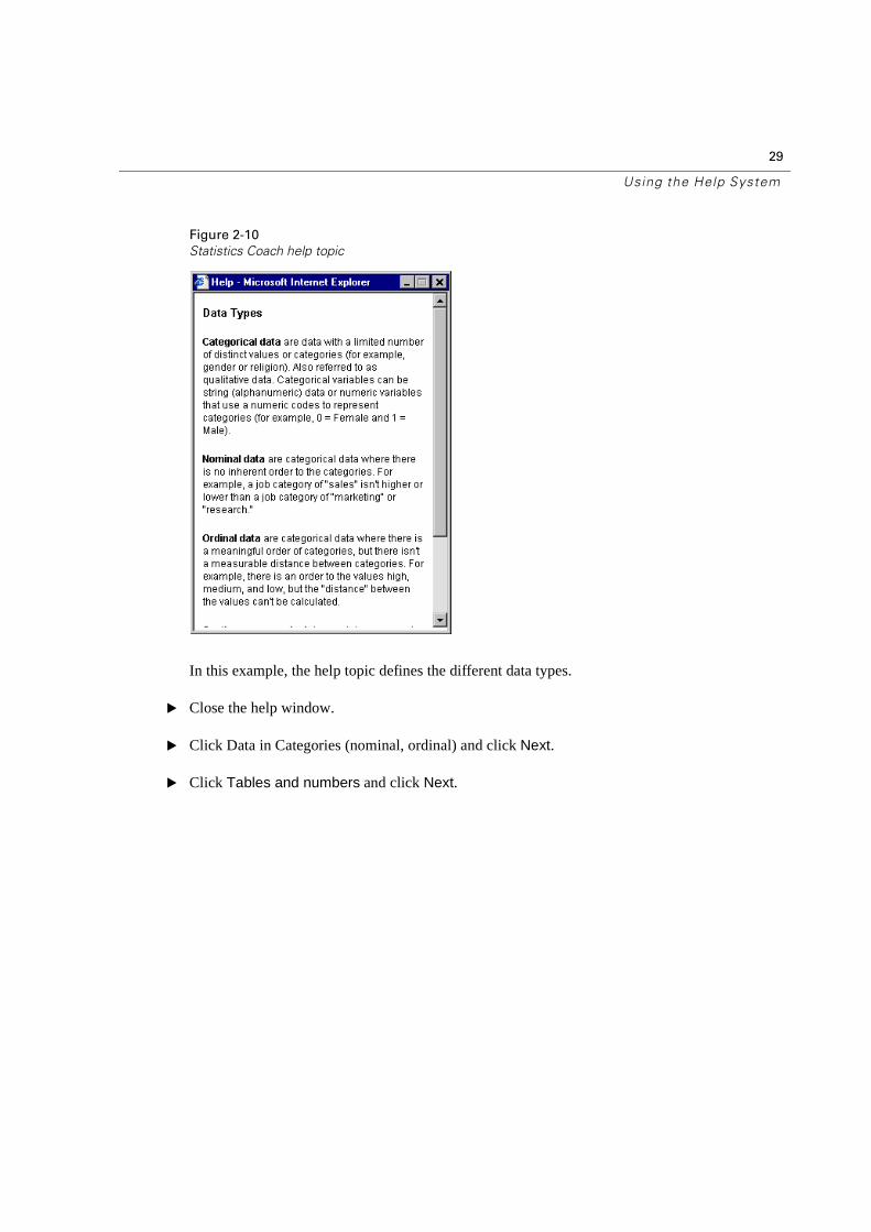
Figure 2-10
Statistics Coach help topic
In this example, the help topic defines the different data types.
� Close the help window.
� Click Data in Categories (nominal, ordinal) and click Next.
� Click Tables and numbers and click Next.
30
Chapter 2
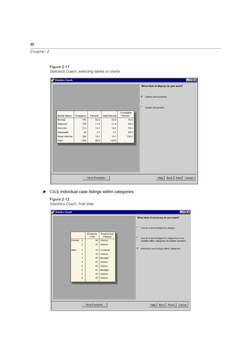
Figure 2-11
Statistics Coach, selecting tables or charts
� Click Individual case listings within categories.
Figure 2-12
Statistics Coach, final step
31
Using the Help System
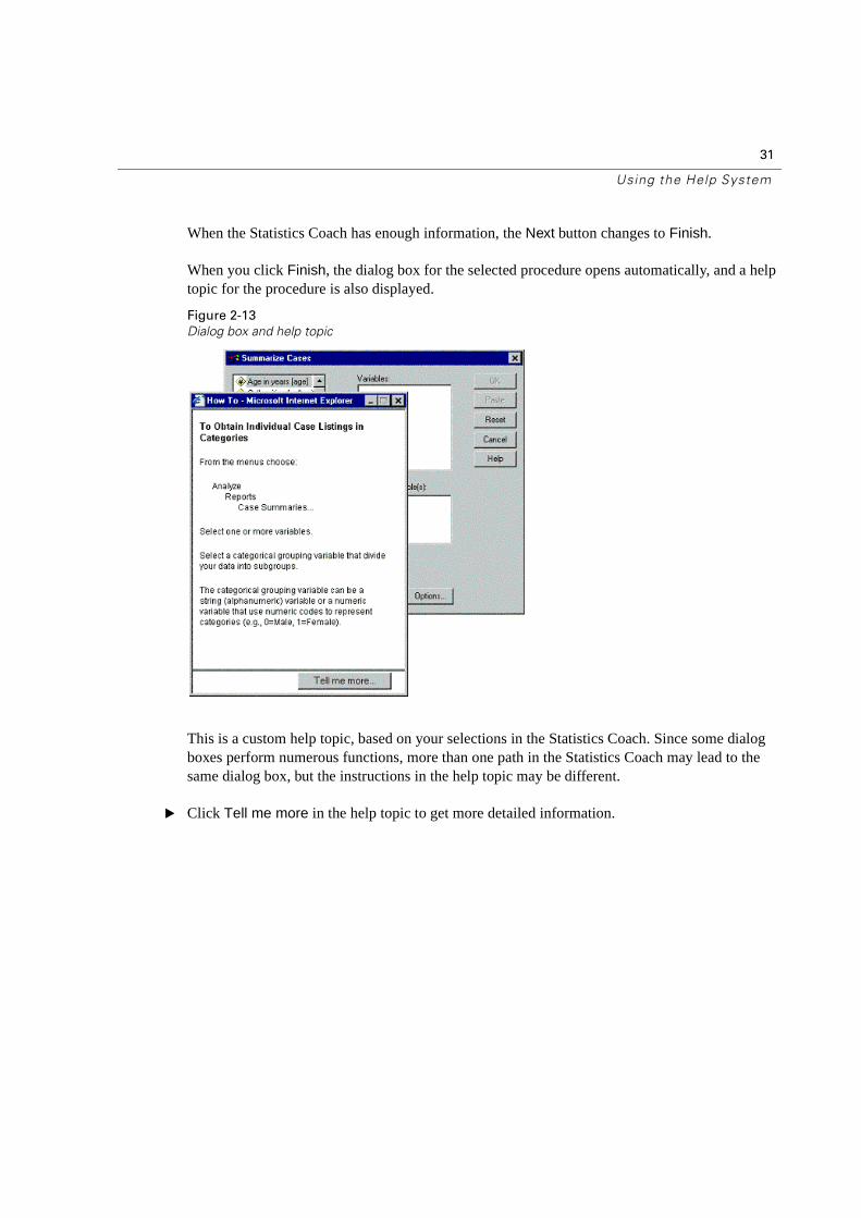
When the Statistics Coach has enough information, the Next button changes to Finish.
When you click Finish, the dialog box for the selected procedure opens automatically, and a help topic for the procedure is also displayed.
Figure 2-13
Dialog box and help topic
This is a custom help topic, based on your selections in the Statistics Coach. Since some dialog boxes perform numerous functions, more than one path in the Statistics Coach may lead to the same dialog box, but the instructions in the help topic may be different.
� Click Tell me more in the help topic to get more detailed information.
32
Chapter 2
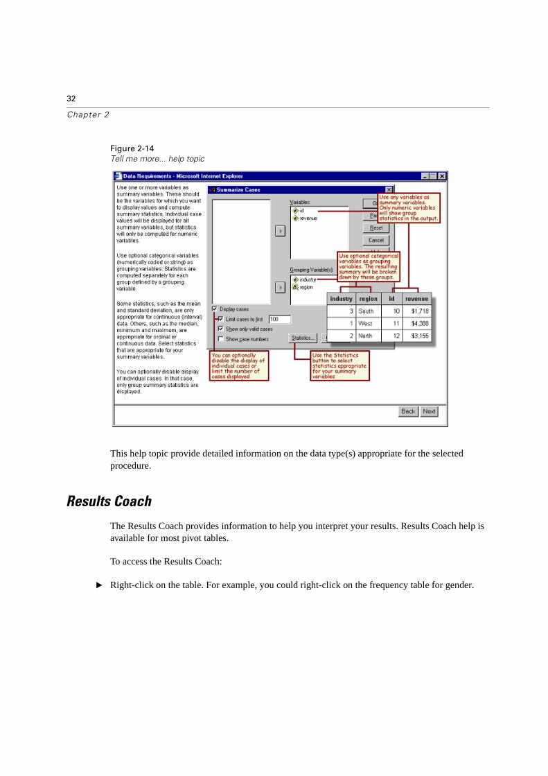
Figure 2-14
Tell me more... help topic
This help topic provide detailed information on the data type(s) appropriate for the selected procedure.
Results Coach
The Results Coach provides information to help you interpret your results. Results Coach help is available for most pivot tables.
To access the Results Coach:
� Right-click on the table. For example, you could right-click on the frequency table for gender.
33
Using the Help System
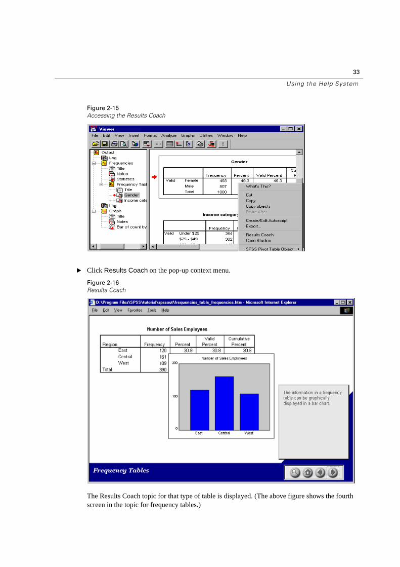
Figure 2-15
Accessing the Results Coach
� Click Results Coach on the pop-up context menu.
Figure 2-16
Results Coach
The Results Coach topic for that type of table is displayed. (The above figure shows the fourth screen in the topic for frequency tables.)
34
Chapter 2
Case Studies
Case Studies provide comprehensive overviews of each procedure. Data files used in the examples are installed with SPSS; so you can follow along performing the same analysis, from opening the data source and selecting variables for analysis to interpreting the results.
To access Case Studies:
� Right-click on any pivot table created by a procedure. For example, you could right-click on the frequency table for gender.
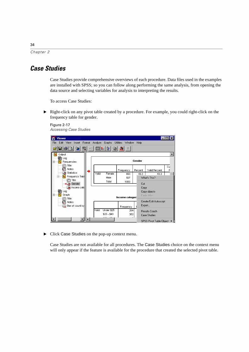
Figure 2-17
Accessing Case Studies
� Click Case Studies on the pop-up context menu.
Case Studies are not available for all procedures. The Case Studies choice on the context menu will only appear if the feature is available for the procedure that created the selected pivot table.
35
Chapte r
3Sources and Organization of Data
Introduction
In this chapter, we discuss common sources of data used for statistical analysis and the preferred data structure. We also discuss issues concerning the coding survey responses in order that analytic software can be applied.
Perhaps the most difficult part of carrying out a research project is obtaining useful data. Often you may have good questions to ask, but finding the correct data to answer the questions is not always easy. This chapter opens with a brief discussion of issues related to gathering data for a research project. There are numerous sources of data available to the insightful researcher. Quite often the data you need to address a specific issue may already be available. We will introduce the various options available with SPSS for reading in the data from some of these sources.
When secondary data (data previously collected by others) do not answer the questions being asked or are simply not available, it may be necessary to collect your own data. This process is expensive and time consuming, so it is critical that the methods used for collecting data are efficient and effective for obtaining the information you need. Part of this chapter will focus on survey research and using surveys as your primary source of data.
Sources of Data
Carol H. Weiss, in her book on evaluation research, states that the only limits on sources and techniques for data collection are the ingenuity and imagination of the researcher (Carol H. Weiss, Evaluation Research, 1972). In the real world there may be other limitations than one’simagination. When beginning a research project the source of data you select for your analysis will be determined by a number of intervening factors such as the resources available for collecting data, time constraints, or the exact data that you need are just not available anywhere. When these factors or a host of others preclude original data collection, you may need to turn to other sources.
36
Chapter 3
Below is a partial list of sources of data:
� Interviews
� Questionnaires
� Observation
� Ratings (by peers, staff, experts)
� Psychometric tests of attitudes, values, personality, preferences, norms, beliefs
� Institutional records
� Government statistics
� Tests of information, interpretation, skills, application of knowledge
� Projective tests
� Situational tests presenting the respondent with simulated life situations
� Diary records
� Physical evidence
� Clinical examinations
� Financial records
� Documents (minutes of board meetings, newspapers, transcripts, etc.)
This list is by no means exhaustive. It is only to provide you with some ideas of available sources of data. The research objectives, the resources available, and a strong dose of ingenuity and imagination will guide you in selecting methods.
Data Organization in SPSS
Before considering the actual data to be used in this course, it might be useful to discuss the general way in which SPSS organizes data.
Rows
If you think of a data file residing in the Data View tab sheet of the Data Editor window, each row corresponds to a unit to be analyzed. For a survey of individuals, each row would represent a respondent. In a data file containing information on Fortune 500 companies, each row would correspond to a company. In a scientific experiment, each row might correspond to a single recorded observation. For sales summary data, each row might correspond to a time unit (for example, one month).
Columns
Each column in the Data Editor corresponds to a specific measurement or type of recorded information. In many areas of research, these measurements are called variables, in some engineering fields they are called characteristics. If in an interview we record five pieces of
37
Sources and Organizat ion of Data
information from each individual, we would have five variables, or columns of data. If in a manufacturing process we record time of day, pH and temperature of a chemical process, we have three variables. Those using survey instruments should be aware that the number of variables or columns might be greater than the number of questions in a survey. This would occur if questions have several parts, or if multiple responses to a single question are permitted.
While there are exceptions to the general rules above (if the same individual is measured at two time points, should the data be placed in one row or two? Answer: it depends on the analysis, but if you wish to look at change at the individual level there should be only one row per individual), thinking about data in this way will facilitate your use of SPSS for Windows.
Design a Coding Scheme
Most data values used for analysis can be read as numbers or strings (alphanumeric). If your data were stored in a database, then each variable, or field as it would be called in the database, would have a declared type (for example: integer, real, or string). When SPSS reads data directly from a database, it maintains the original types as best it can. If you are collecting and entering the data yourself, then you must decide how to code the data for the analysis.
Data sources originally coded as numbers are easy to analyze; however, to analyze other data sources, for example survey questions that have more than one alternative, you must develop a coding scheme. A coding scheme is a way to associate a particular data code with a response. The codes are what you enter into a data file.
Coding schemes are arbitrary. For example, a gender question could be coded with a zero (0) for male and a one (1) for female. Or, the coding scheme could assign an “m” for male and an “f”for female. Either way is acceptable for SPSS. Whenever possible it is recommended that a coding scheme consist of numbers rather than alphabetic characters. Some statistical procedures will not work with alpha characters. For example, it is meaningless to get the average of a group of letters. It is more efficient to use numeric codes; however, it is acceptable to use character codes for nominal variables (variables for which each data value represents a category). Also, SPSS can produce numeric codes from string (alphabetic) codes using the AUTORECODE procedure.
Whenever you design a coding scheme for a questionnaire, you should try to figure out all of the possible responses you are interested in and assign a code for each different response.
The computer “crunches” the coded values to create tabulations, perform statistical tests, and draw graphs and charts. To make it easier to read your results, you can instruct SPSS to label the coded values. For example, you can use the code “f” for gender and supply the label “Female.”Another example would be to use the code 1 to indicate the strongly agree survey response and supply the label “Strongly Agree.” We will discuss how to supply such labels to SPSS.
Identification Fields
One thing that you should be sure to do is to have an identification number in the data. This could be a number assigned to each survey questionnaire after it is returned or a code corresponding to each individual in a database. Identification numbers let you identify which survey (or data) form or database record corresponds to which SPSS data record. This facilitates data cleaning and the resolution of data problems.
38
Chapter 3
Choices in Entering Data
If your data are not already stored on a computer, you must decide how to enter the data, for example from a questionnaire, into a file on the computer. Look at the questionnaire form or data sheet and decide how to enter the values. You can decide where to enter the data values for each questionnaire item.
There are various methods of entering the data values. You can use the SPSS Data Editor window, or other software such as spreadsheet or database programs. One of the simplest methods outside of SPSS for small studies is to use a text editor such as the Windows Notepad and type the values in a columnar sequence. Here, when a response is missing, you can enter blanks by pressing the space bar and move to the columns for the next item. For high-volume processing of surveys, you might consider scanning the survey responses. Products such as Remark Office OMR and Teleform allow you to design survey forms that can be later scanned to record the responses.
SPSS Data Entry
An alternative method involves software dedicated to data entry, such as the SPSS Data Entry program. Using this program you can design a survey form on the screen, enter responses using the form as a guide, and create an SPSS data file. It allows for validity checking and permits skip and fill rules. Programs such as SPSS Data Entry, allow surveys to be posted to web sites and data collected through the Internet.
Extensions
For more information on the design and development of surveys, SPSS offers a Survey Methodology training course. Analyses typically performed on survey data are reviewed in the Survey Analysis with SPSS training course. Instruction on designing a survey instrument using SPSS Data Entry is covered in the Introduction to Data Entry training course.
Summary
In this chapter we discussed issues involving sources of data and organization of data for analysis by SPSS. In addition, methods of coding survey data that facilitate statistical analysis within SPSS were reviewed.
39
Sources and Organizat ion of Data
Appendix: Sample Data from an Engineering Application
To demonstrate that most of the same data organization and coding issues arise in studies involving physical, biological and health sciences, and engineering, we describe a data set used in a statistical process control study of voltage output from motors in a manufacturing plant.
The plant builds electric motors whose output is designed to be 350 volts with specification limits of +/- 5 volts. Recent process control testing found motors outside of the specification limit, and in order to investigate possible causes, data were collected from motors produced during different shifts, with wire obtained from different suppliers, and on different machines. Each row of data represents a motor that was tested and contains codes for shift, wire supplier and machine, as well as the voltage measure.
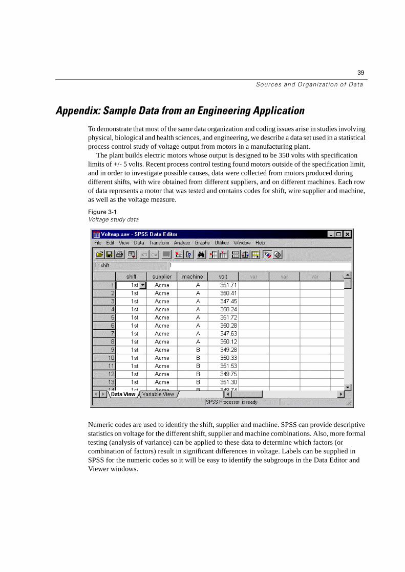
Figure 3-1
Voltage study data
Numeric codes are used to identify the shift, supplier and machine. SPSS can provide descriptive statistics on voltage for the different shift, supplier and machine combinations. Also, more formal testing (analysis of variance) can be applied to these data to determine which factors (or combination of factors) result in significant differences in voltage. Labels can be supplied in SPSS for the numeric codes so it will be easy to identify the subgroups in the Data Editor and Viewer windows.

41
Chapte r
4Reading Data
Reading Data
Data can be entered directly into SPSS, or it can be imported from a number of different sources. The processes for reading data stored in SPSS data files, spreadsheet applications like Microsoft Excel, database applications like Microsoft Access, and text files are all discussed in this chapter.
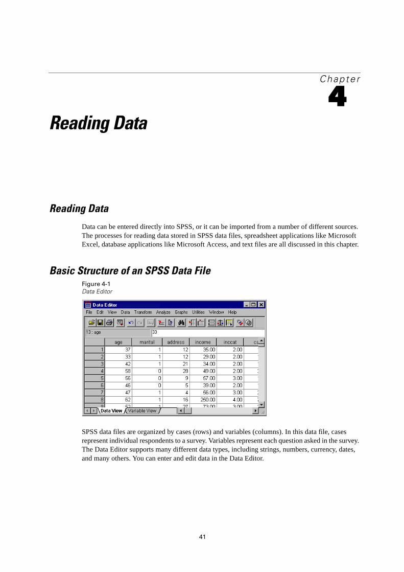
Basic Structure of an SPSS Data FileFigure 4-1
Data Editor
SPSS data files are organized by cases (rows) and variables (columns). In this data file, cases represent individual respondents to a survey. Variables represent each question asked in the survey. The Data Editor supports many different data types, including strings, numbers, currency, dates, and many others. You can enter and edit data in the Data Editor.
42
Chapter 4
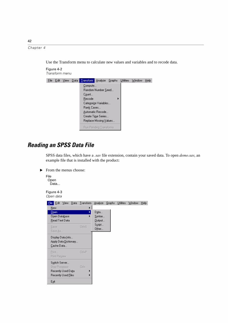
Use the Transform menu to calculate new values and variables and to recode data.
Figure 4-2
Transform menu
Reading an SPSS Data File
SPSS data files, which have a .sav file extension, contain your saved data. To open demo.sav, an example file that is installed with the product:
� From the menus choose:
FileOpen
Data...
Figure 4-3
Open data
43
Reading Data
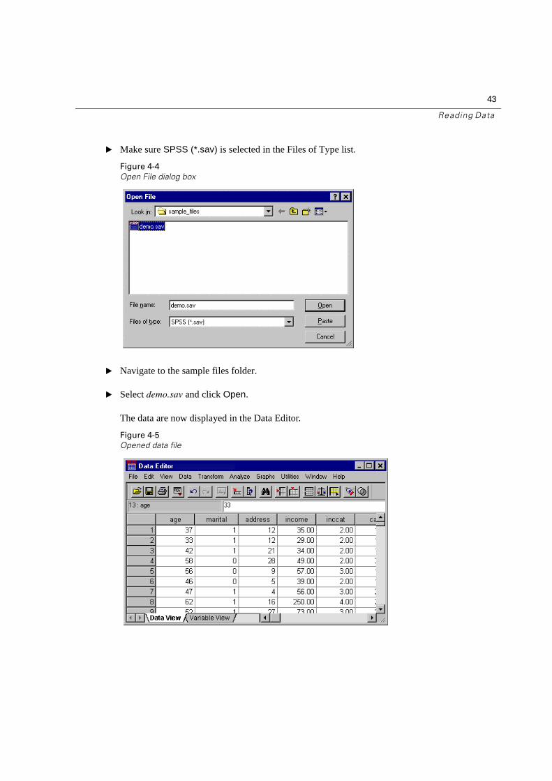
� Make sure SPSS (*.sav) is selected in the Files of Type list.
Figure 4-4
Open File dialog box
� Navigate to the sample files folder.
� Select demo.sav and click Open.
The data are now displayed in the Data Editor.
Figure 4-5
Opened data file
44
Chapter 4
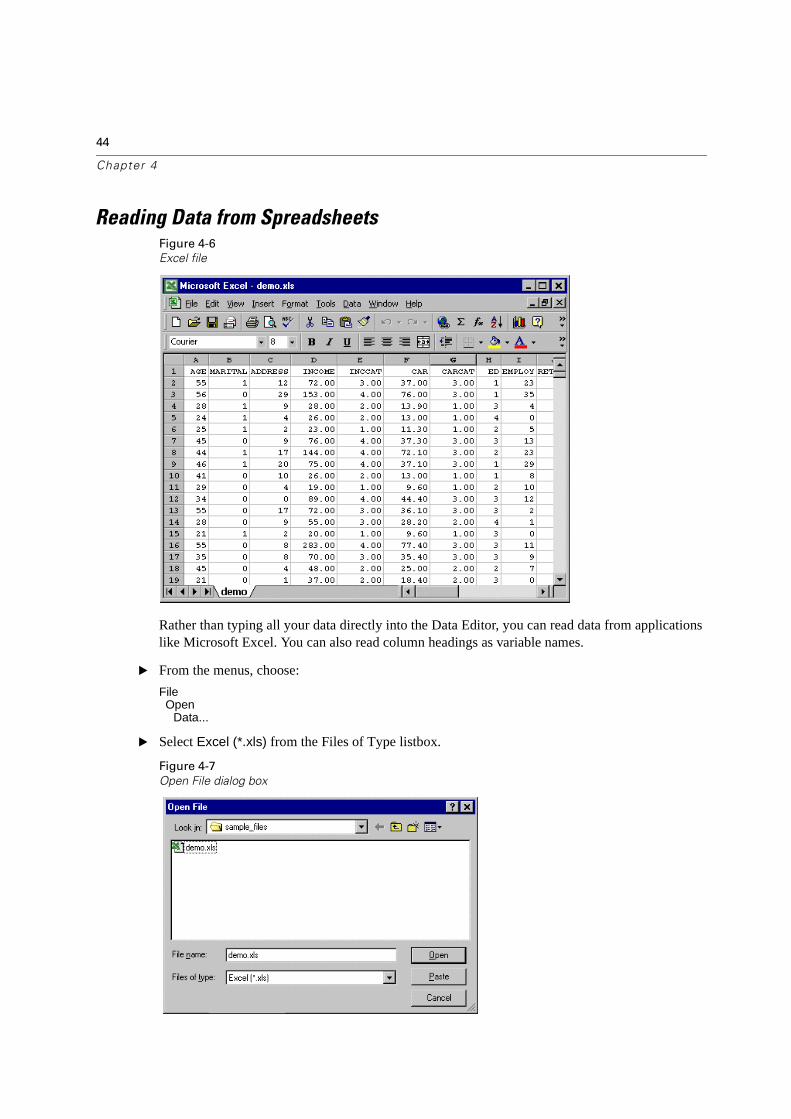
Reading Data from SpreadsheetsFigure 4-6
Excel file
Rather than typing all your data directly into the Data Editor, you can read data from applications like Microsoft Excel. You can also read column headings as variable names.
� From the menus, choose:
FileOpen
Data...
� Select Excel (*.xls) from the Files of Type listbox.
Figure 4-7
Open File dialog box
45
Reading Data
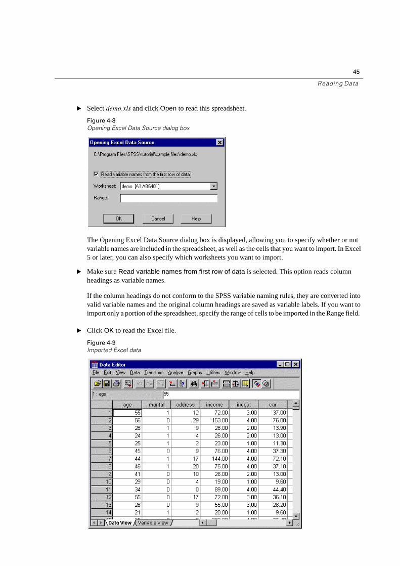
� Select demo.xls and click Open to read this spreadsheet.
Figure 4-8
Opening Excel Data Source dialog box
The Opening Excel Data Source dialog box is displayed, allowing you to specify whether or not variable names are included in the spreadsheet, as well as the cells that you want to import. In Excel 5 or later, you can also specify which worksheets you want to import.
� Make sure Read variable names from first row of data is selected. This option reads column headings as variable names.
If the column headings do not conform to the SPSS variable naming rules, they are converted into valid variable names and the original column headings are saved as variable labels. If you want to import only a portion of the spreadsheet, specify the range of cells to be imported in the Range field.
� Click OK to read the Excel file.
Figure 4-9
Imported Excel data
46
Chapter 4
The data now appear in the Data Editor, with the column headings used as variable names. If you’reusing a spreadsheet application other than Excel or Lotus, it should be able to export your data to a supported format that can then be read into SPSS.
Reading Data from a Database
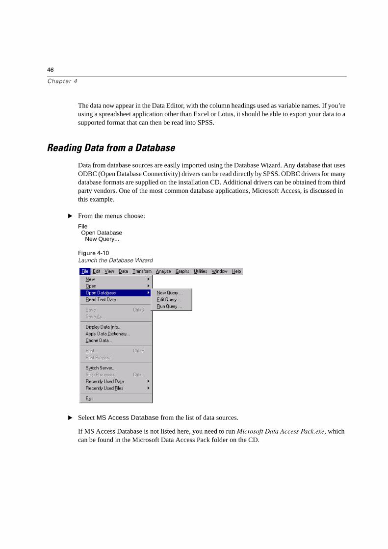
Data from database sources are easily imported using the Database Wizard. Any database that uses ODBC (Open Database Connectivity) drivers can be read directly by SPSS. ODBC drivers for many database formats are supplied on the installation CD. Additional drivers can be obtained from third party vendors. One of the most common database applications, Microsoft Access, is discussed in this example.
� From the menus choose:
FileOpen Database
New Query...
Figure 4-10
Launch the Database Wizard
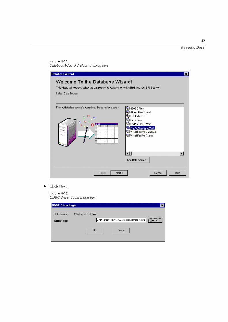
� Select MS Access Database from the list of data sources.
If MS Access Database is not listed here, you need to run Microsoft Data Access Pack.exe, which can be found in the Microsoft Data Access Pack folder on the CD.
47
Reading Data
Figure 4-11
Database Wizard Welcome dialog box
� Click Next.
Figure 4-12
ODBC Driver Login dialog box
48
Chapter 4
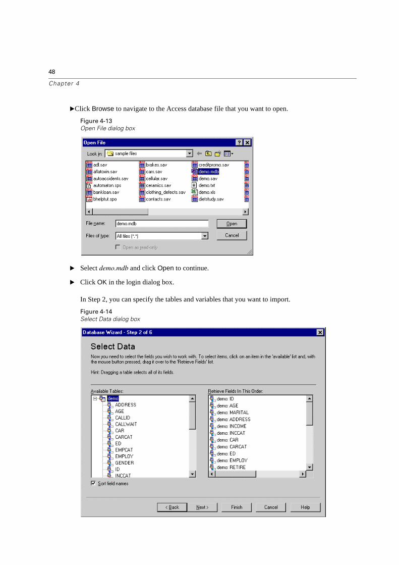
�Click Browse to navigate to the Access database file that you want to open.
Figure 4-13
Open File dialog box
� Select demo.mdb and click Open to continue.
� Click OK in the login dialog box.
In Step 2, you can specify the tables and variables that you want to import.
Figure 4-14
Select Data dialog box
49
Reading Data
� Drag the entire demo table to Retrieve Fields in This Order.
� Click Next.
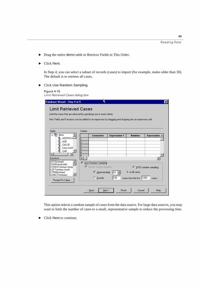
In Step 4, you can select a subset of records (cases) to import (for example, males older than 30). The default is to retrieve all cases.
� Click Use Random Sampling.
Figure 4-15
Limit Retrieved Cases dialog box
This option selects a random sample of cases from the data source. For large data sources, you may want to limit the number of cases to a small, representative sample to reduce the processing time.
� Click Next to continue.
50
Chapter 4
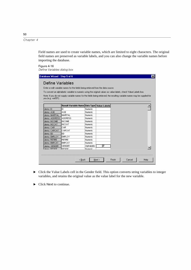
Field names are used to create variable names, which are limited to eight characters. The original field names are preserved as variable labels, and you can also change the variable names before importing the database.
Figure 4-16
Define Variables dialog box
� Click the Value Labels cell in the Gender field. This option converts string variables to integer variables, and retains the original value as the value label for the new variable.
� Click Next to continue.
51
Reading Data
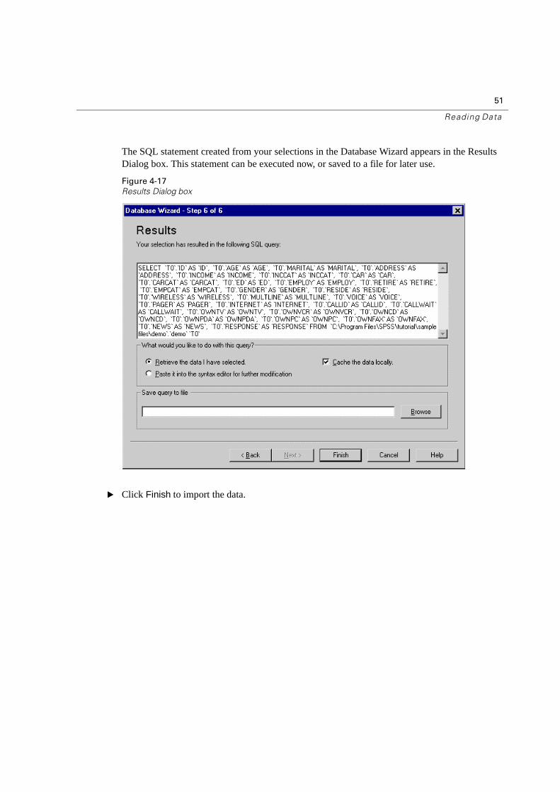
The SQL statement created from your selections in the Database Wizard appears in the Results Dialog box. This statement can be executed now, or saved to a file for later use.
Figure 4-17
Results Dialog box
� Click Finish to import the data.
52
Chapter 4
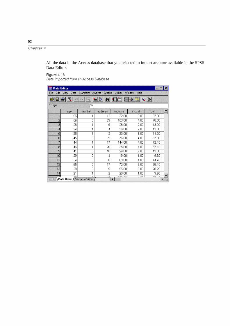
All the data in the Access database that you selected to import are now available in the SPSS Data Editor.
Figure 4-18
Data Imported from an Access Database
53
Reading Data
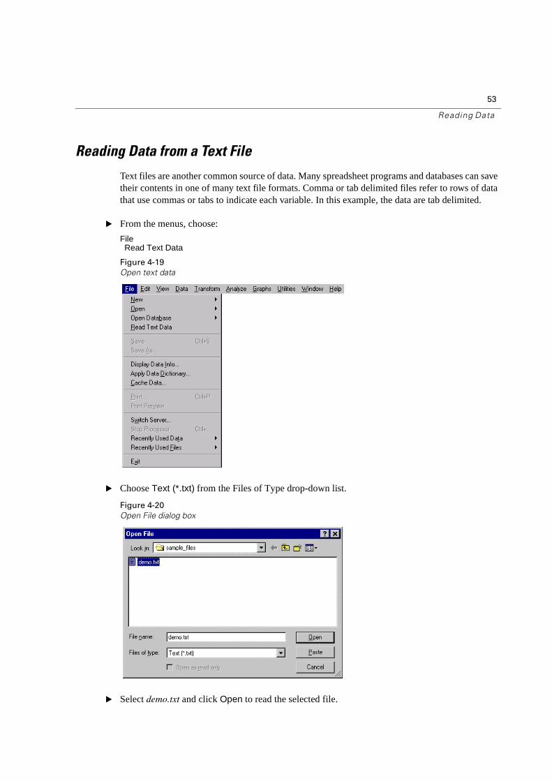
Reading Data from a Text File
Text files are another common source of data. Many spreadsheet programs and databases can save their contents in one of many text file formats. Comma or tab delimited files refer to rows of data that use commas or tabs to indicate each variable. In this example, the data are tab delimited.
� From the menus, choose:
FileRead Text Data
Figure 4-19
Open text data
� Choose Text (*.txt) from the Files of Type drop-down list.
Figure 4-20
Open File dialog box
� Select demo.txt and click Open to read the selected file.
54
Chapter 4
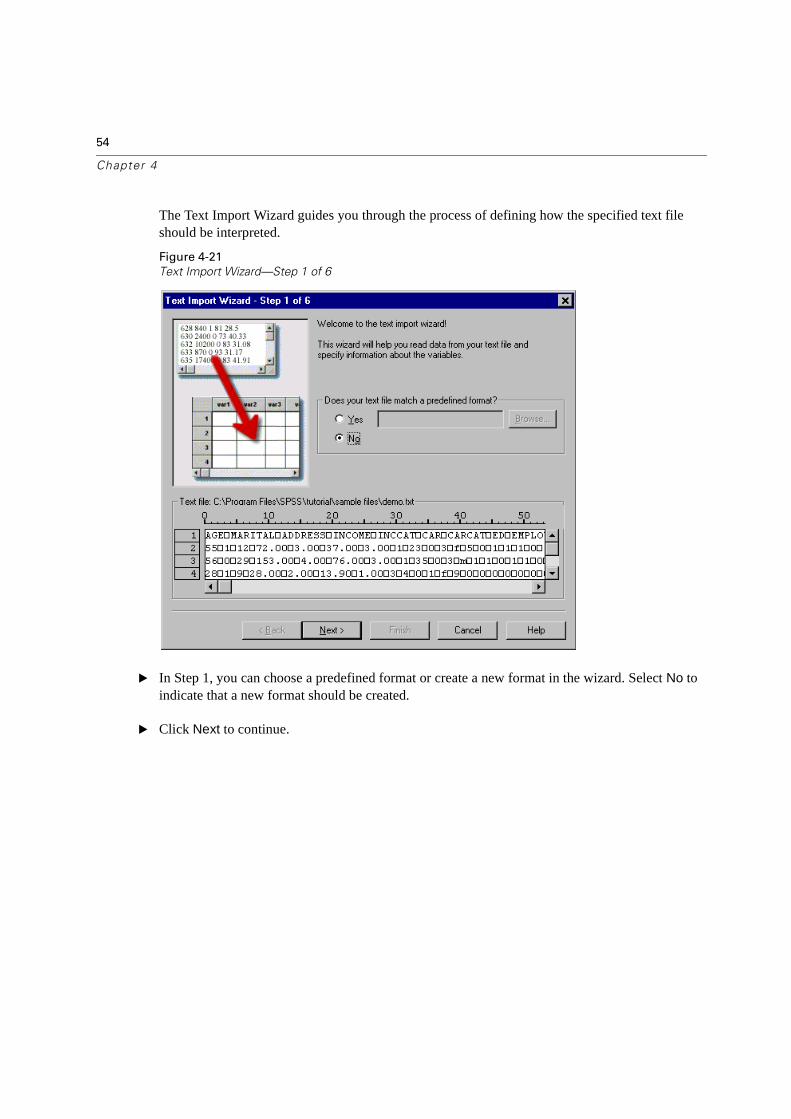
The Text Import Wizard guides you through the process of defining how the specified text file should be interpreted.
Figure 4-21
Text Import Wizard—Step 1 of 6
� In Step 1, you can choose a predefined format or create a new format in the wizard. Select No to indicate that a new format should be created.
� Click Next to continue.
55
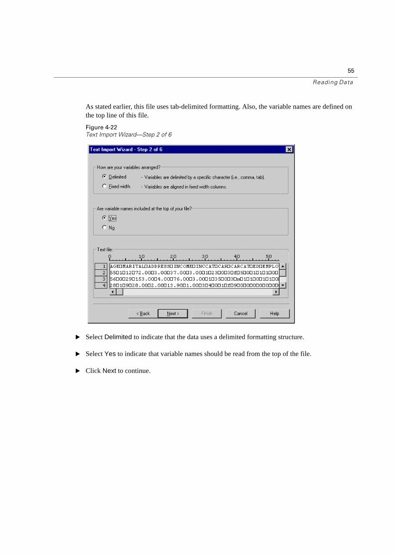
Reading Data
As stated earlier, this file uses tab-delimited formatting. Also, the variable names are defined on the top line of this file.
Figure 4-22
Text Import Wizard—Step 2 of 6
� Select Delimited to indicate that the data uses a delimited formatting structure.
� Select Yes to indicate that variable names should be read from the top of the file.
� Click Next to continue.
56
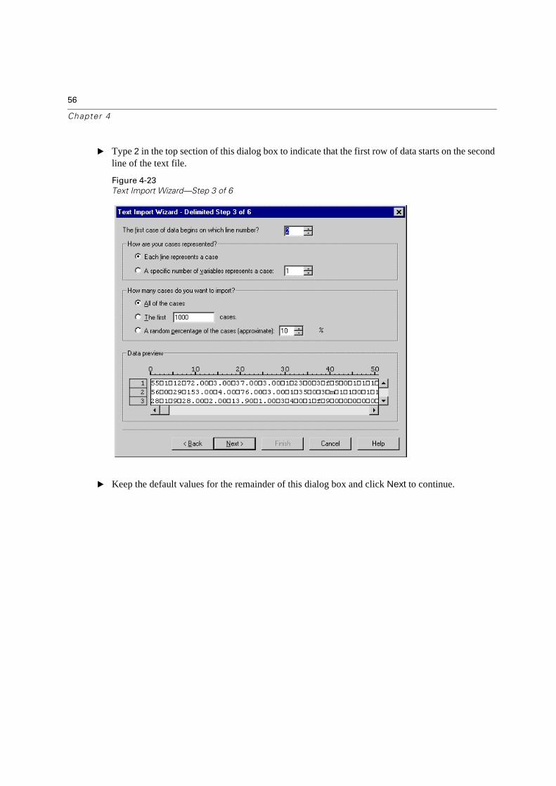
Chapter 4
� Type 2 in the top section of this dialog box to indicate that the first row of data starts on the second line of the text file.
Figure 4-23
Text Import Wizard—Step 3 of 6
� Keep the default values for the remainder of this dialog box and click Next to continue.
57
Reading Data
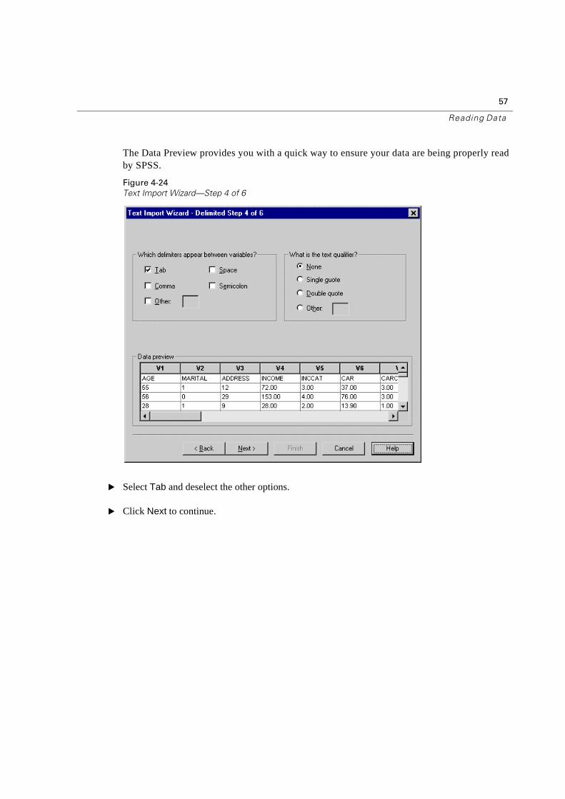
The Data Preview provides you with a quick way to ensure your data are being properly read by SPSS.
Figure 4-24
Text Import Wizard—Step 4 of 6
� Select Tab and deselect the other options.
� Click Next to continue.
58
Chapter 4
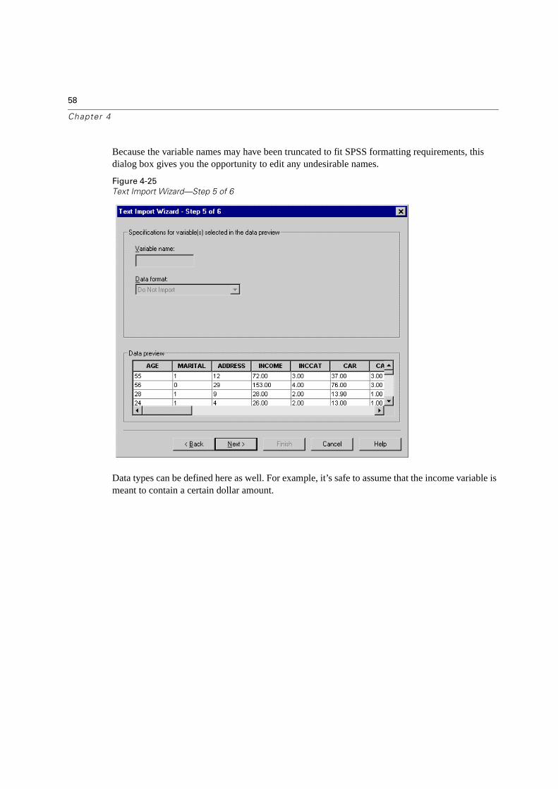
Because the variable names may have been truncated to fit SPSS formatting requirements, this dialog box gives you the opportunity to edit any undesirable names.
Figure 4-25
Text Import Wizard—Step 5 of 6
Data types can be defined here as well. For example, it’s safe to assume that the income variable is meant to contain a certain dollar amount.
59
Reading Data
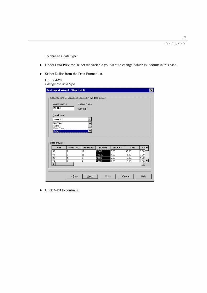
To change a data type:
� Under Data Preview, select the variable you want to change, which is Income in this case.
� Select Dollar from the Data Format list.
Figure 4-26
Change the data type
� Click Next to continue.
60
Chapter 4
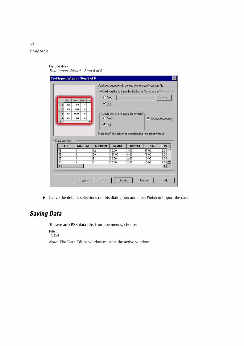
Figure 4-27
Text Import Wizard—Step 6 of 6
� Leave the default selections on this dialog box and click Finish to import the data.
Saving Data
To save an SPSS data file, from the menus, choose:
FileSave
Note: The Data Editor window must be the active window.
61
Reading Data
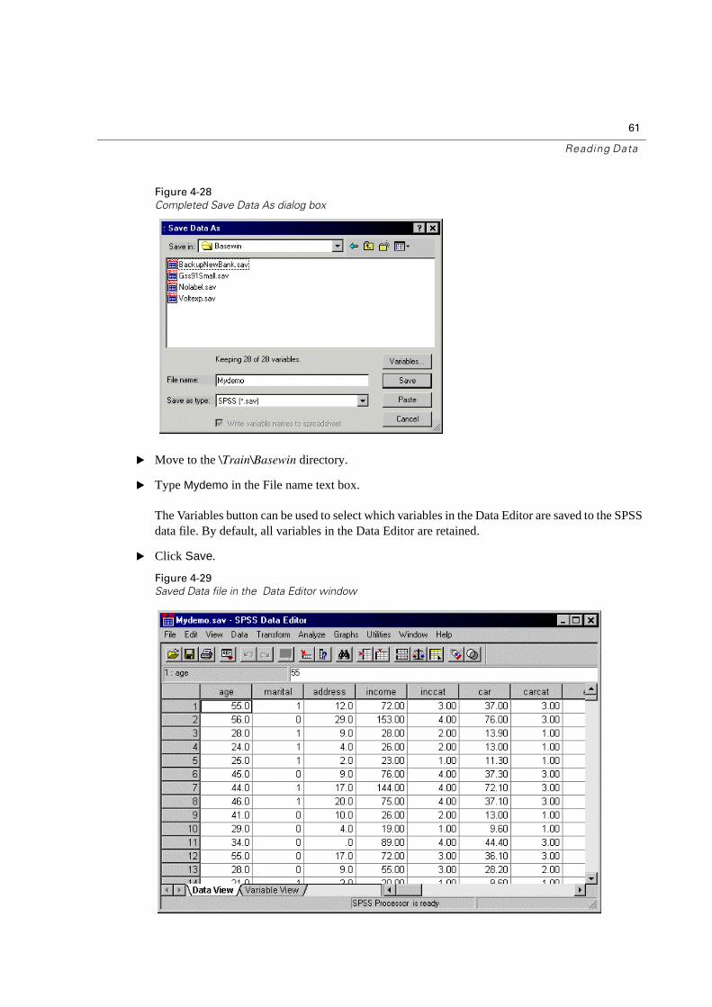
Figure 4-28
Completed Save Data As dialog box
� Move to the \Train\Basewin directory.
� Type Mydemo in the File name text box.
The Variables button can be used to select which variables in the Data Editor are saved to the SPSS data file. By default, all variables in the Data Editor are retained.
� Click Save.
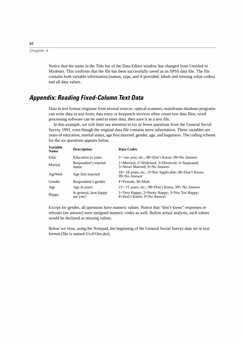
Figure 4-29
Saved Data file in the Data Editor window
62
Chapter 4
Notice that the name in the Title bar of the Data Editor window has changed from Untitled to Mydemo. This confirms that the file has been successfully saved as an SPSS data file. The file contains both variable information (names, type, and if provided, labels and missing value codes) and all data values.
Appendix: Reading Fixed-Column Text Data
Data in text format originate from several sources: optical scanners; mainframe database programs can write data in text form; data entry or keypunch services often create text data files; word processing software can be used to enter data, then save it as a text file.
In this example, we will limit our attention to six or fewer questions from the General Social Survey 1991, even though the original data file contains more information. These variables are years of education, marital status, age first married, gender, age, and happiness. The coding scheme for the six questions appears below.
Except for gender, all questions have numeric values. Notice that “don’t know” responses or refusals (no answer) were assigned numeric codes as well. Before actual analysis, such values would be declared as missing values.
Below we view, using the Notepad, the beginning of the General Social Survey data set in text format (file is named Gss91Sm.dat).
Variable Name Description Data Codes
Educ Education in years 1= one year, etc.; 98=Don’t Know; 99=No Answer
Marital Respondent’s marital status
1=Married; 2=Widowed; 3=Divorced; 4=Separated;5=Never Married; 9=No Answer
AgeWed Age first married 18= 18 years, etc.; 0=Not Applicable; 98=Don’t Know; 99=No Answer
Gender Respondent’s gender F=Female; M=Male
Age Age in years 21= 21 years, etc.; 98=Don’t Know; 99= No Answer
Happy In general, how happy are you?
1=Very Happy; 2=Pretty Happy; 3=Not Too Happy; 8=Don’t Know; 9=No Answer
63
Reading Data
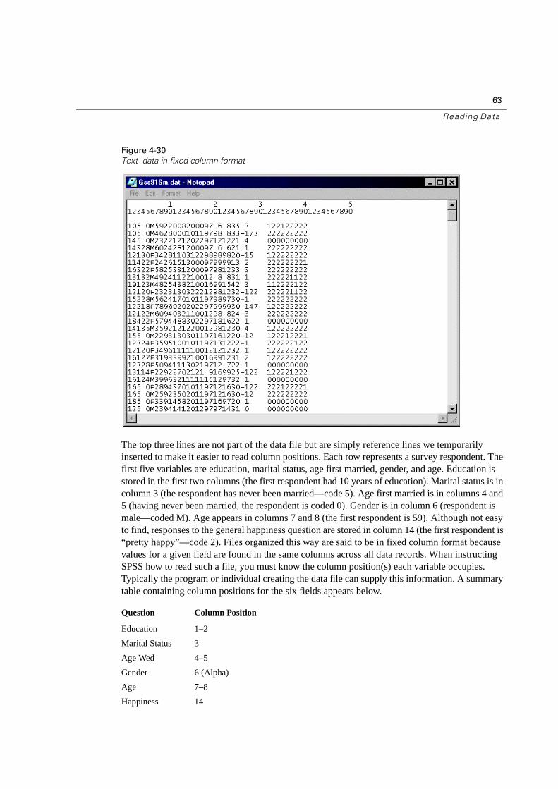
Figure 4-30
Text data in fixed column format
The top three lines are not part of the data file but are simply reference lines we temporarily inserted to make it easier to read column positions. Each row represents a survey respondent. The first five variables are education, marital status, age first married, gender, and age. Education is stored in the first two columns (the first respondent had 10 years of education). Marital status is in column 3 (the respondent has never been married—code 5). Age first married is in columns 4 and 5 (having never been married, the respondent is coded 0). Gender is in column 6 (respondent is male—coded M). Age appears in columns 7 and 8 (the first respondent is 59). Although not easy to find, responses to the general happiness question are stored in column 14 (the first respondent is “pretty happy”—code 2). Files organized this way are said to be in fixed column format because values for a given field are found in the same columns across all data records. When instructing SPSS how to read such a file, you must know the column position(s) each variable occupies. Typically the program or individual creating the data file can supply this information. A summary table containing column positions for the six fields appears below.
Question Column Position
Education 1–2
Marital Status 3
Age Wed 4–5
Gender 6 (Alpha)
Age 7–8
Happiness 14
64
Chapter 4
� To read text data, from the menus, choose:
FileRead Text Data
We must first identify the data file to be read by SPSS and then define each data field that we want SPSS to process.
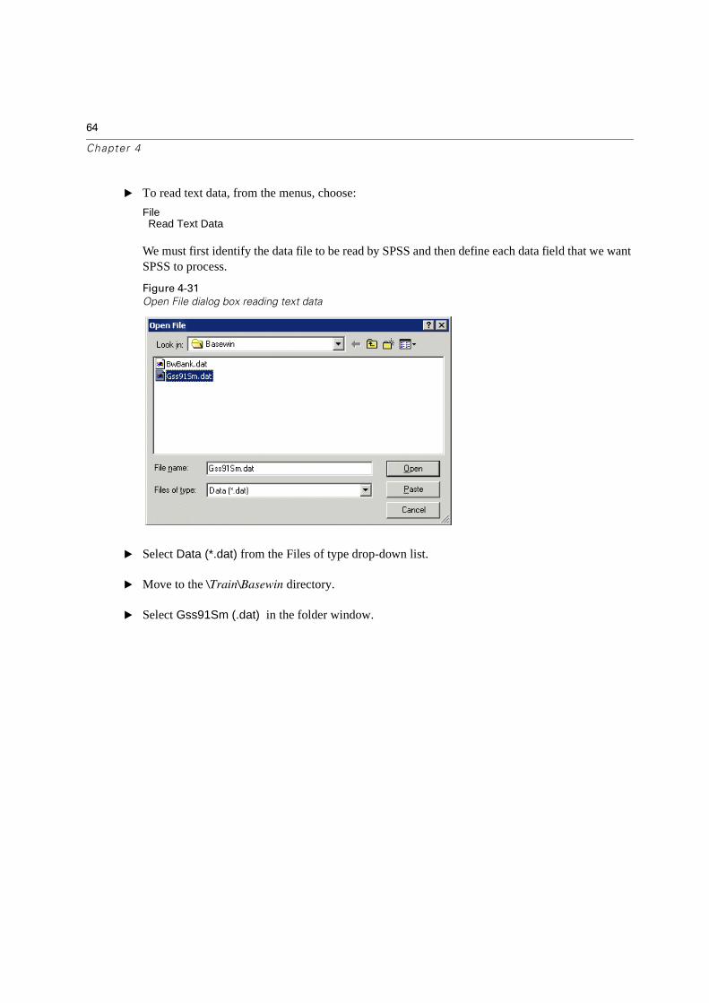
Figure 4-31
Open File dialog box reading text data
� Select Data (*.dat) from the Files of type drop-down list.
� Move to the \Train\Basewin directory.
� Select Gss91Sm (.dat) in the folder window.
65
Reading Data
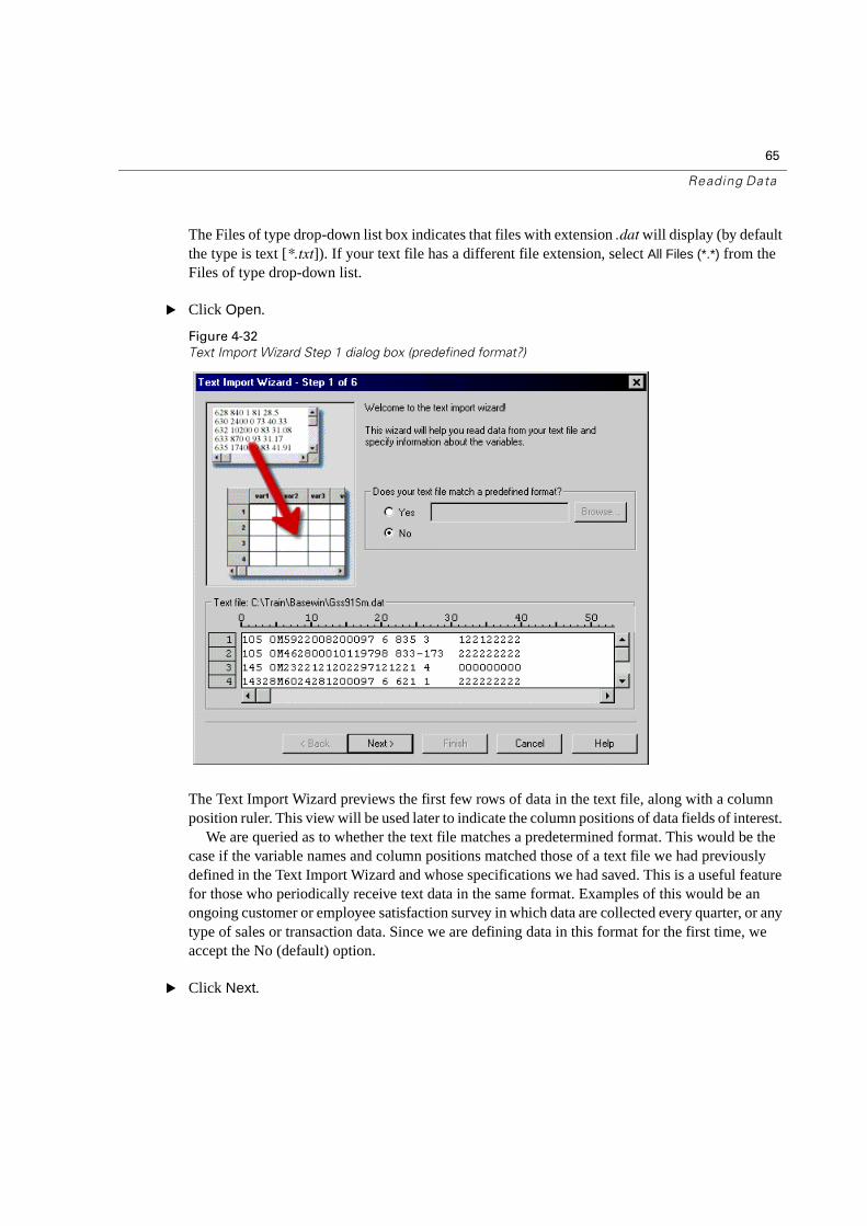
The Files of type drop-down list box indicates that files with extension .dat will display (by default the type is text [*.txt]). If your text file has a different file extension, select All Files (*.*) from the Files of type drop-down list.
� Click Open.
Figure 4-32
Text Import Wizard Step 1 dialog box (predefined format?)
The Text Import Wizard previews the first few rows of data in the text file, along with a column position ruler. This view will be used later to indicate the column positions of data fields of interest.
We are queried as to whether the text file matches a predetermined format. This would be the case if the variable names and column positions matched those of a text file we had previously defined in the Text Import Wizard and whose specifications we had saved. This is a useful feature for those who periodically receive text data in the same format. Examples of this would be an ongoing customer or employee satisfaction survey in which data are collected every quarter, or any type of sales or transaction data. Since we are defining data in this format for the first time, we accept the No (default) option.
� Click Next.
66
Chapter 4
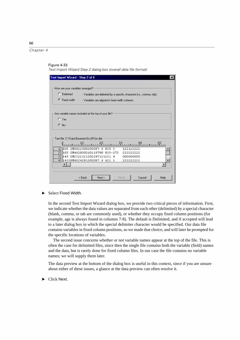
Figure 4-33
Text Import Wizard Step 2 dialog box (overall data file format)
� Select Fixed Width.
In the second Text Import Wizard dialog box, we provide two critical pieces of information. First, we indicate whether the data values are separated from each other (delimited) by a special character (blank, comma, or tab are commonly used), or whether they occupy fixed column positions (for example, age is always found in columns 7-8). The default is Delimited, and if accepted will lead to a later dialog box in which the special delimiter character would be specified. Our data file contains variables in fixed column positions, so we made that choice, and will later be prompted for the specific locations of variables.
The second issue concerns whether or not variable names appear at the top of the file. This is often the case for delimited files, since then the single file contains both the variable (field) names and the data, but is rarely done for fixed column files. In our case the file contains no variable names; we will supply them later.
The data preview at the bottom of the dialog box is useful in this context, since if you are unsure about either of these issues, a glance at the data preview can often resolve it.
� Click Next.
67
Reading Data
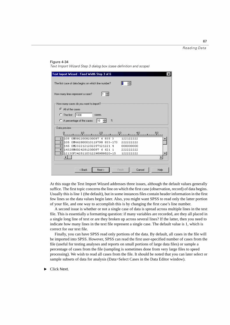
Figure 4-34
Text Import Wizard Step 3 dialog box (case definition and scope)
At this stage the Text Import Wizard addresses three issues, although the default values generally suffice. The first topic concerns the line on which the first case (observation, record) of data begins. Usually this is line 1 (the default), but in some instances files contain header information in the first few lines so the data values begin later. Also, you might want SPSS to read only the latter portion of your file, and one way to accomplish this is by changing the first case’s line number.
A second issue is whether or not a single case of data is spread across multiple lines in the text file. This is essentially a formatting question: if many variables are recorded, are they all placed in a single long line of text or are they broken up across several lines? If the latter, then you need to indicate how many lines in the text file represent a single case. The default value is 1, which is correct for our text file.
Finally, you can have SPSS read only portions of the data. By default, all cases in the file will be imported into SPSS. However, SPSS can read the first user-specified number of cases from the file (useful for testing analyses and reports on small portions of large data files) or sample a percentage of cases from the file (sampling is sometimes done from very large files to speed processing). We wish to read all cases from the file. It should be noted that you can later select or sample subsets of data for analysis (Data>Select Cases in the Data Editor window).
� Click Next.
68
Chapter 4
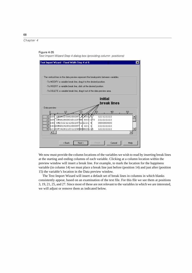
Figure 4-35
Text Import Wizard Step 4 dialog box (providing column positions)
We now must provide the column locations of the variables we wish to read by inserting break lines at the starting and ending columns of each variable. Clicking at a column location within the preview window will insert a break line. For example, to mark the location for the happiness variable (in column 14) we must place a break line just before (position 14) and just after (position 15) the variable’s location in the Data preview window.
The Text Import Wizard will insert a default set of break lines in columns in which blanks consistently appear, based on an examination of the text file. For this file we see them at positions 3, 19, 21, 25, and 27. Since most of these are not relevant to the variables in which we are interested, we will adjust or remove them as indicated below.
69
Reading Data
We begin by defining the columns for the education variable (columns 1–2).
� Click below position 2 in the preview window (just after the 10 at the beginning of the first line of data).
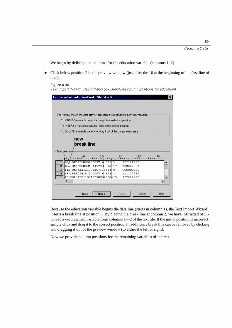
Figure 4-36
Text Import Wizard Step 4 dialog box (supplying column positions for education)
Because the education variable begins the data line (starts in column 1), the Text Import Wizard inserts a break line at position 0. By placing the break line at column 2, we have instructed SPSS to read a yet unnamed variable from columns 1—2 of the text file. If the initial position is incorrect, simply click and drag it to the correct position. In addition, a break line can be removed by clicking and dragging it out of the preview window (to either the left or right).
Now we provide column positions for the remaining variables of interest.
70
Chapter 4
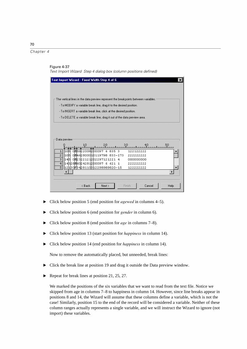
Figure 4-37
Text Import Wizard Step 4 dialog box (column positions defined)
� Click below position 5 (end position for agewed in columns 4–5).
� Click below position 6 (end position for gender in column 6).
� Click below position 8 (end position for age in columns 7–8).
� Click below position 13 (start position for happiness in column 14).
� Click below position 14 (end position for happiness in column 14).
Now to remove the automatically placed, but unneeded, break lines:
� Click the break line at position 19 and drag it outside the Data preview window.
� Repeat for break lines at position 21, 25, 27.
We marked the positions of the six variables that we want to read from the text file. Notice we skipped from age in columns 7–8 to happiness in column 14. However, since line breaks appear in positions 8 and 14, the Wizard will assume that these columns define a variable, which is not the case! Similarly, position 15 to the end of the record will be considered a variable. Neither of these column ranges actually represents a single variable, and we will instruct the Wizard to ignore (not import) these variables.
71
Reading Data
After allowing for the exceptions just noted, we defined six of the many data fields contained in the text file. Thus you have the flexibility of reading only fields of interest.
� Click Next.
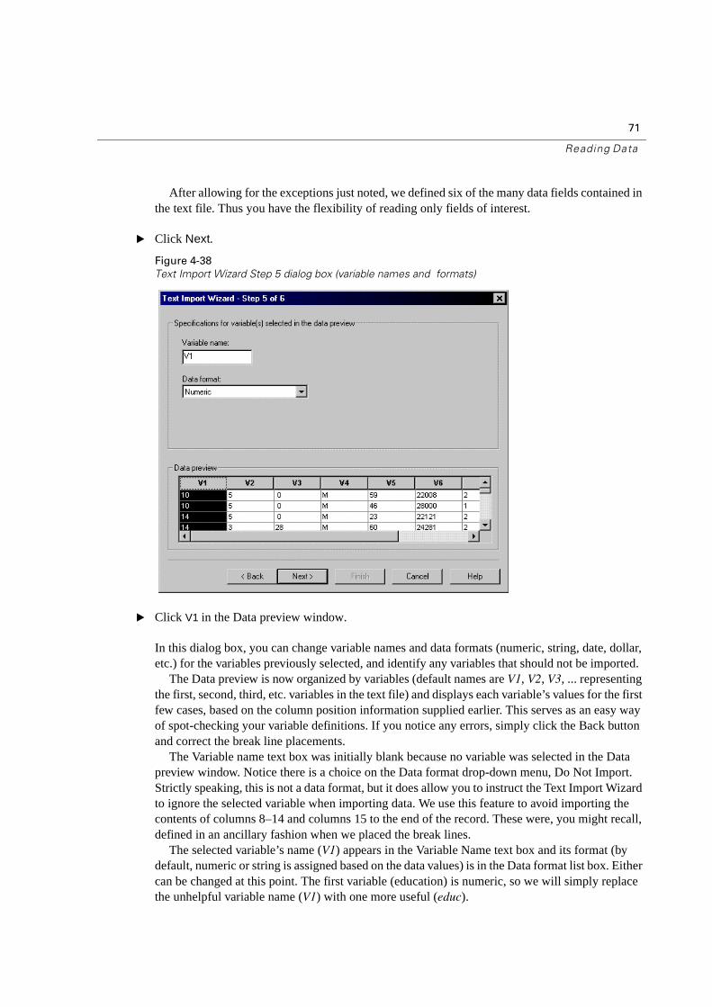
Figure 4-38
Text Import Wizard Step 5 dialog box (variable names and formats)
� Click V1 in the Data preview window.
In this dialog box, you can change variable names and data formats (numeric, string, date, dollar, etc.) for the variables previously selected, and identify any variables that should not be imported.
The Data preview is now organized by variables (default names are V1, V2, V3, ... representing the first, second, third, etc. variables in the text file) and displays each variable’s values for the first few cases, based on the column position information supplied earlier. This serves as an easy way of spot-checking your variable definitions. If you notice any errors, simply click the Back button and correct the break line placements.
The Variable name text box was initially blank because no variable was selected in the Data preview window. Notice there is a choice on the Data format drop-down menu, Do Not Import. Strictly speaking, this is not a data format, but it does allow you to instruct the Text Import Wizard to ignore the selected variable when importing data. We use this feature to avoid importing the contents of columns 8–14 and columns 15 to the end of the record. These were, you might recall, defined in an ancillary fashion when we placed the break lines.
The selected variable’s name (V1) appears in the Variable Name text box and its format (by default, numeric or string is assigned based on the data values) is in the Data format list box. Either can be changed at this point. The first variable (education) is numeric, so we will simply replace the unhelpful variable name (V1) with one more useful (educ).
72
Chapter 4
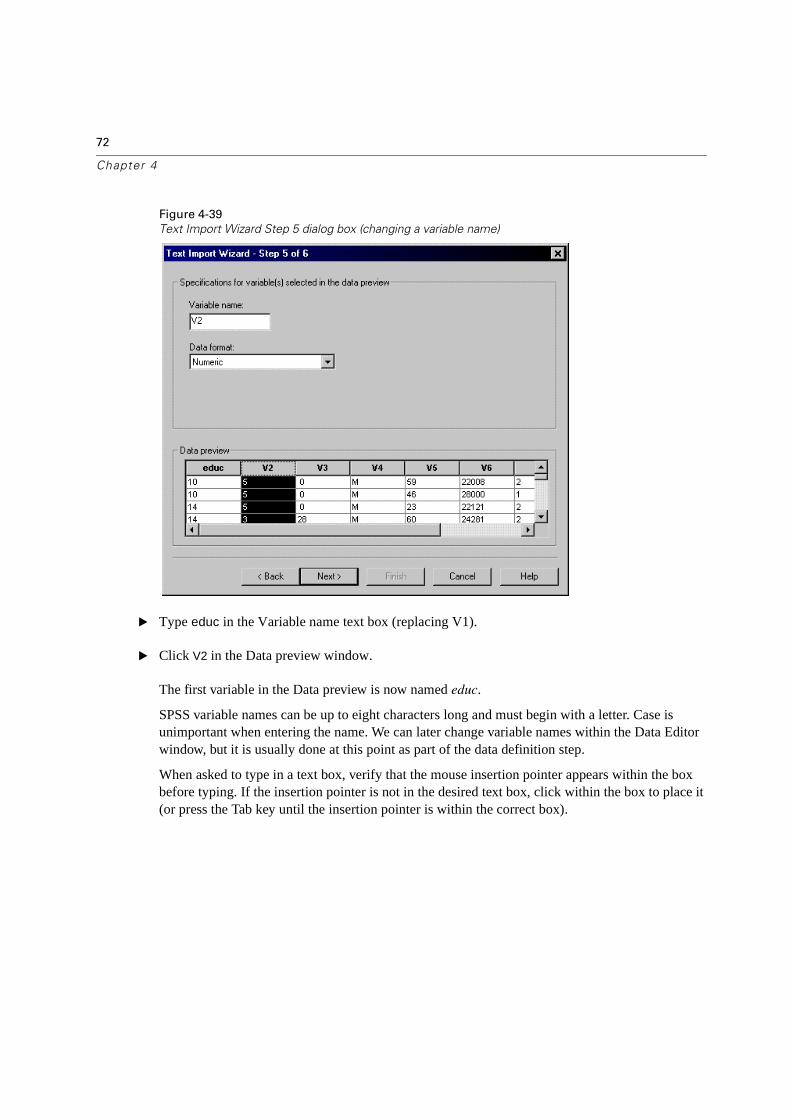
Figure 4-39
Text Import Wizard Step 5 dialog box (changing a variable name)
� Type educ in the Variable name text box (replacing V1).
� Click V2 in the Data preview window.
The first variable in the Data preview is now named educ.
SPSS variable names can be up to eight characters long and must begin with a letter. Case is unimportant when entering the name. We can later change variable names within the Data Editor window, but it is usually done at this point as part of the data definition step.
When asked to type in a text box, verify that the mouse insertion pointer appears within the box before typing. If the insertion pointer is not in the desired text box, click within the box to place it (or press the Tab key until the insertion pointer is within the correct box).
73
Reading Data
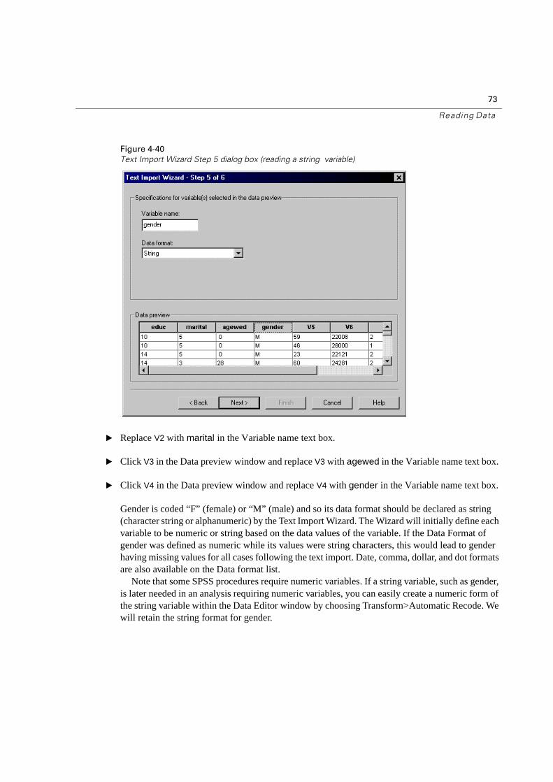
Figure 4-40
Text Import Wizard Step 5 dialog box (reading a string variable)
� Replace V2 with marital in the Variable name text box.
� Click V3 in the Data preview window and replace V3 with agewed in the Variable name text box.
� Click V4 in the Data preview window and replace V4 with gender in the Variable name text box.
Gender is coded “F” (female) or “M” (male) and so its data format should be declared as string (character string or alphanumeric) by the Text Import Wizard. The Wizard will initially define each variable to be numeric or string based on the data values of the variable. If the Data Format of gender was defined as numeric while its values were string characters, this would lead to gender having missing values for all cases following the text import. Date, comma, dollar, and dot formats are also available on the Data format list.
Note that some SPSS procedures require numeric variables. If a string variable, such as gender, is later needed in an analysis requiring numeric variables, you can easily create a numeric form of the string variable within the Data Editor window by choosing Transform>Automatic Recode. We will retain the string format for gender.
74
Chapter 4
To continue:
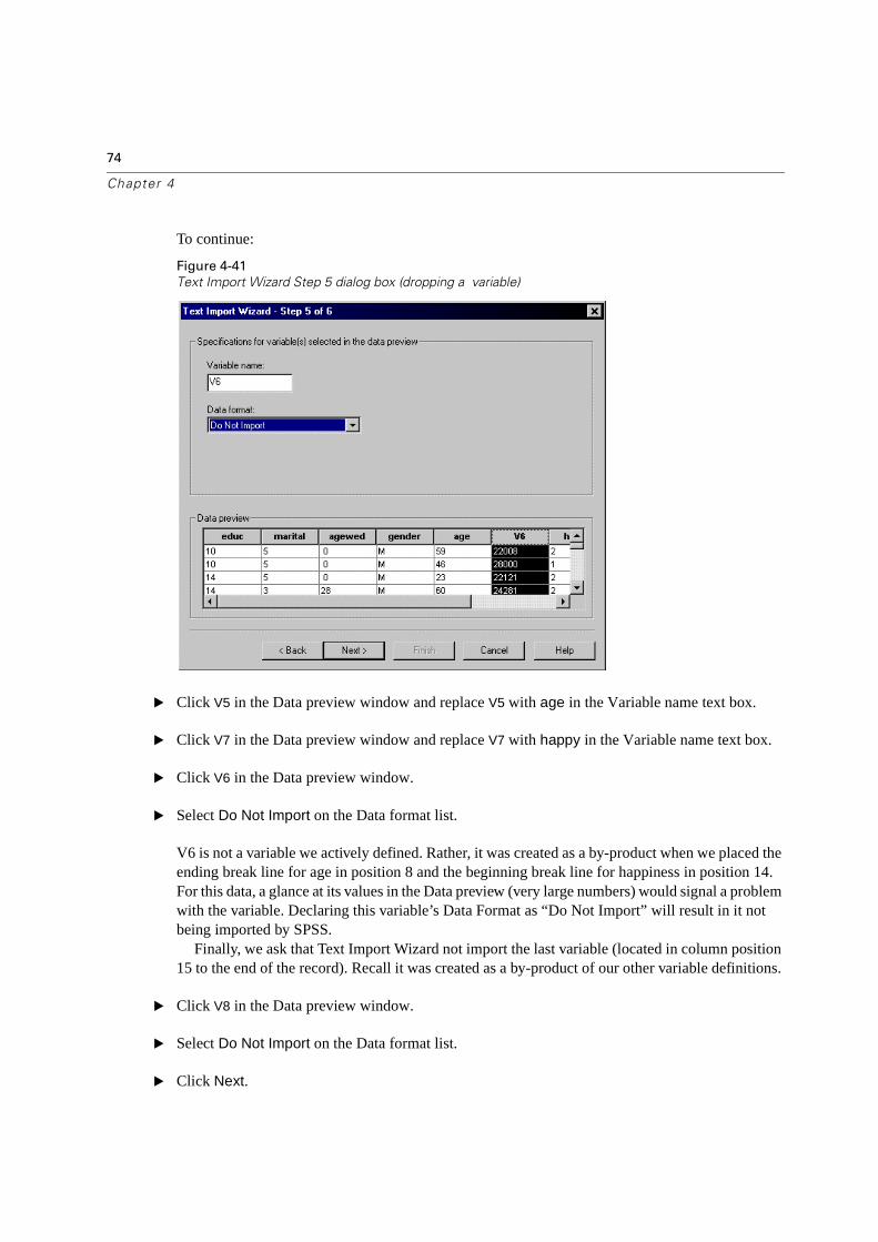
Figure 4-41
Text Import Wizard Step 5 dialog box (dropping a variable)
� Click V5 in the Data preview window and replace V5 with age in the Variable name text box.
� Click V7 in the Data preview window and replace V7 with happy in the Variable name text box.
� Click V6 in the Data preview window.
� Select Do Not Import on the Data format list.
V6 is not a variable we actively defined. Rather, it was created as a by-product when we placed the ending break line for age in position 8 and the beginning break line for happiness in position 14. For this data, a glance at its values in the Data preview (very large numbers) would signal a problem with the variable. Declaring this variable’s Data Format as “Do Not Import” will result in it not being imported by SPSS.
Finally, we ask that Text Import Wizard not import the last variable (located in column position 15 to the end of the record). Recall it was created as a by-product of our other variable definitions.
� Click V8 in the Data preview window.
� Select Do Not Import on the Data format list.
� Click Next.
75
Reading Data
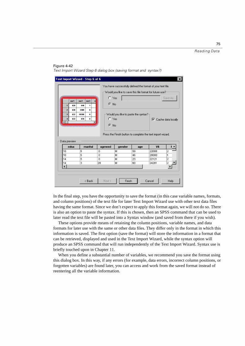
Figure 4-42
Text Import Wizard Step 6 dialog box (saving format and syntax?)
In the final step, you have the opportunity to save the format (in this case variable names, formats, and column positions) of the text file for later Text Import Wizard use with other text data files having the same format. Since we don’t expect to apply this format again, we will not do so. There is also an option to paste the syntax. If this is chosen, then an SPSS command that can be used to later read the text file will be pasted into a Syntax window (and saved from there if you wish).
These options provide means of retaining the column positions, variable names, and data formats for later use with the same or other data files. They differ only in the format in which this information is saved. The first option (save the format) will store the information in a format that can be retrieved, displayed and used in the Text Import Wizard, while the syntax option will produce an SPSS command that will run independently of the Text Import Wizard. Syntax use is briefly touched upon in Chapter 11.
When you define a substantial number of variables, we recommend you save the format using this dialog box. In this way, if any errors (for example, data errors, incorrect column positions, or forgotten variables) are found later, you can access and work from the saved format instead of reentering all the variable information.
76
Chapter 4
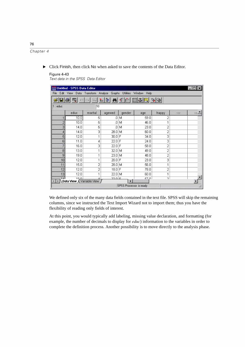
� Click Finish, then click No when asked to save the contents of the Data Editor.
Figure 4-43
Text data in the SPSS Data Editor
We defined only six of the many data fields contained in the text file. SPSS will skip the remaining columns, since we instructed the Text Import Wizard not to import them; thus you have the flexibility of reading only fields of interest.
At this point, you would typically add labeling, missing value declaration, and formatting (for example, the number of decimals to display for educ) information to the variables in order to complete the definition process. Another possibility is to move directly to the analysis phase.
77
Chapte r
5Using the Data Editor
Using the Data Editor
The Data Editor displays the contents of the active data file. The information in the Data Editor consists of variables and cases.
� In Data View, columns represent variables and rows represent cases (observations).
� In Variable View, each row is a variable, and each column is an attribute associated with that variable.
Variables are used to represent the different types of data you have compiled. A common analogy is that of a survey. The response to each question on a survey is equivalent to a variable. Variables come in many different types, including numbers, strings, currency, and dates.
Entering Numeric Data
Data can be typed into the Data Editor, which may be useful for small data files or making minor edits to larger data files.
� Click the Variable View tab at the bottom of the Data Editor window.
Define the variables that are going to be used. In this case, only three variables are needed: age,marital status, and income.
78
Chapter 5
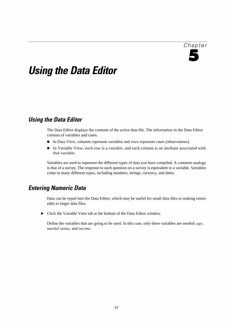
Figure 5-1
Variable names
� In the first row of the first column, type age.
� In the second row, type marital.
� In the third row, type income.
New variables are automatically given a numeric data type.
If you don’t enter variable names, unique names are automatically created. However, these names are not descriptive and are not recommended for large data files.
� Click the Data View tab to continue entering the data.
The names you entered in the Variable View are now the headings for the first three columns of the Data View.
Begin entering data in the first row, starting at the first column.
79
Using the Data Editor
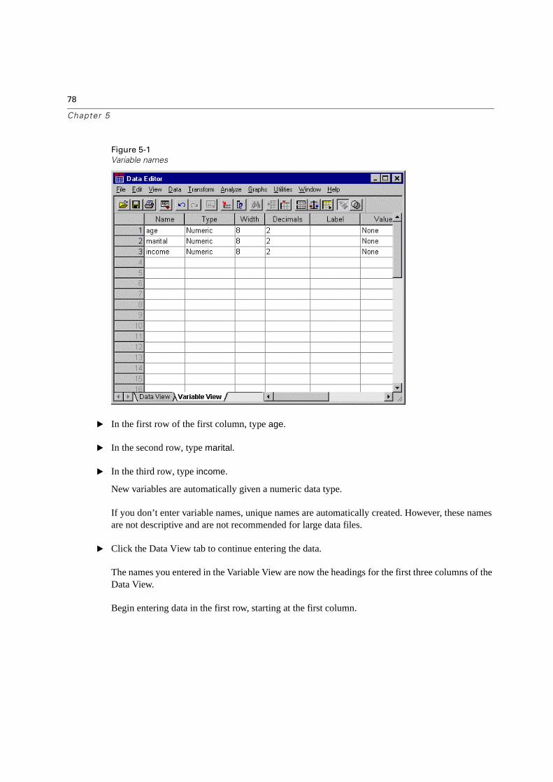
Figure 5-2
Data View
� In the age column, type 55.
� In the marital column, type 1.
� In the income column, type 72000.
� Move the cursor to the first column of the second row to add the next subject’s data.
� In the age column, type 53.
� In the marital column, type 0.
� In the income column, type 153000.
80
Chapter 5
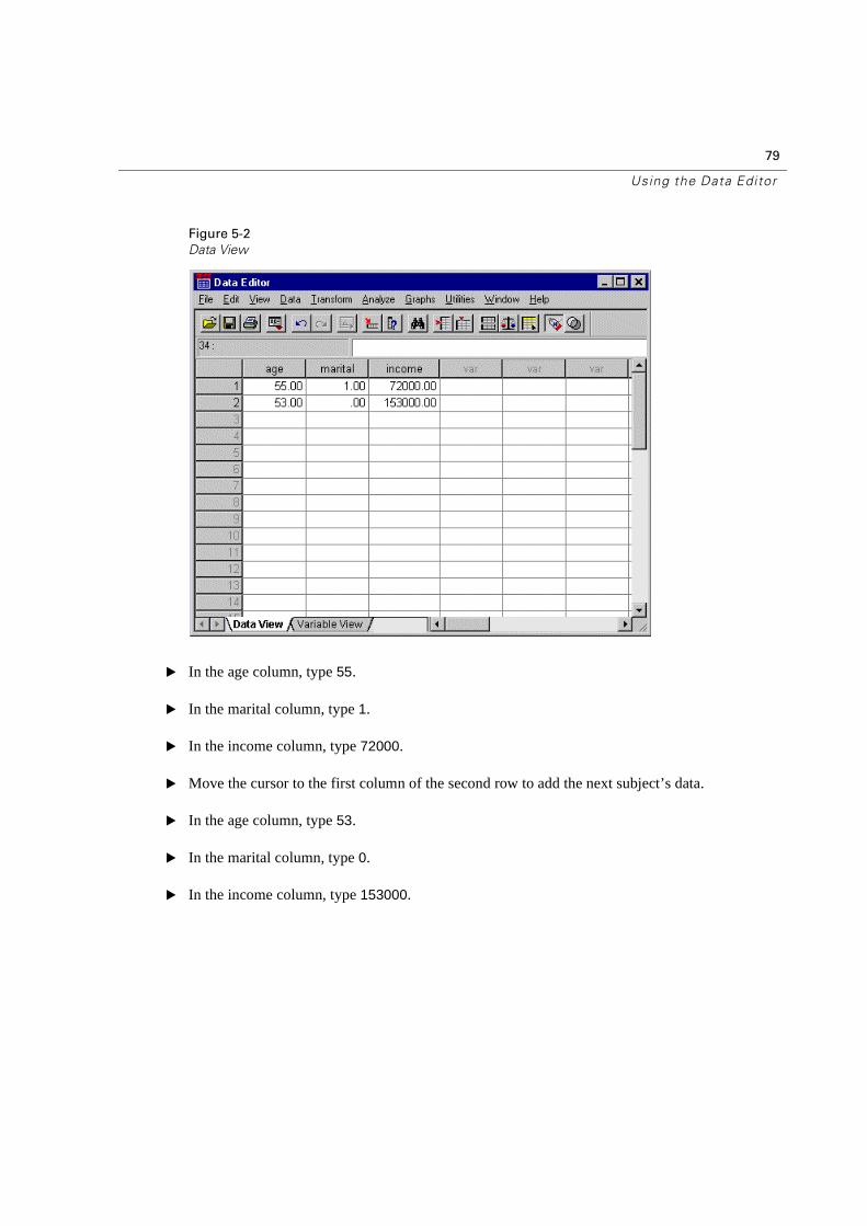
Currently, the age and marital columns display decimal points, even though their values are intended to be integers. To hide the decimal points in these variables...
� Click the Variable View tab at the bottom of the Data Editor window.
� Select the Decimals column in the age row and type 0 to hide the decimal.
� Select the Decimals column in the marital row and type 0 to hide the decimal.
Figure 5-3
Setting the decimal for age
Entering String Data
Non-numeric data, such as strings of text, can also be entered in the Data Editor.
� Click the Variable View tab at the bottom of the Data Editor window.
� In the first cell of the first blank row, type sex for the variable name.
� Click the Type cell.
81
Using the Data Editor
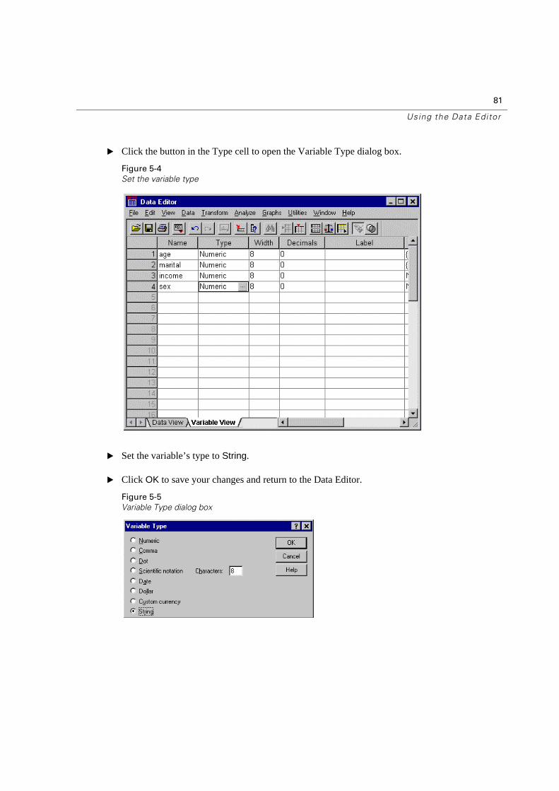
� Click the button in the Type cell to open the Variable Type dialog box.
Figure 5-4
Set the variable type
� Set the variable’s type to String.
� Click OK to save your changes and return to the Data Editor.
Figure 5-5
Variable Type dialog box
82
Chapter 5
Defining Data
In addition to defining data types, you can also define descriptive variable and value labels for variable names and data values. These descriptive labels are used in statistical reports and charts.
Adding a Variable Label
Labels are meant to provide descriptions of variables. These descriptions are often longer versions of variable names. Variable names can be only eight characters long, which is usually too short for a descriptive and readable name. Labels can be up to 256 characters long. These labels are used in your output to identify the different variables.
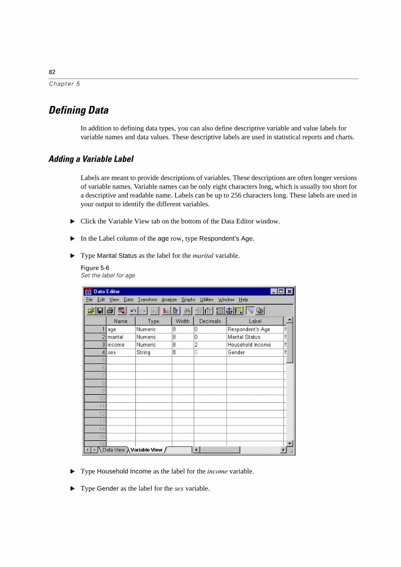
� Click the Variable View tab on the bottom of the Data Editor window.
� In the Label column of the age row, type Respondent’s Age.
� Type Marital Status as the label for the marital variable.
Figure 5-6
Set the label for age
� Type Household Income as the label for the income variable.
� Type Gender as the label for the sex variable.
83
Using the Data Editor
Changing Variable Type and Format
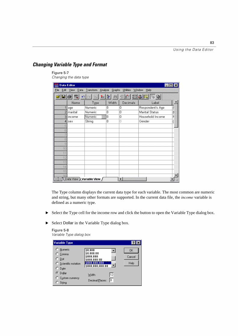
Figure 5-7
Changing the data type
The Type column displays the current data type for each variable. The most common are numeric and string, but many other formats are supported. In the current data file, the income variable is defined as a numeric type.
� Select the Type cell for the income row and click the button to open the Variable Type dialog box.
� Select Dollar in the Variable Type dialog box.
Figure 5-8
Variable Type dialog box
84
Chapter 5
The formatting options for the currently selected data type are displayed.
� Select the format of this currency. For this example, select $###,###,###.
� Click OK to implement your changes.
Adding Value Labels for Numeric Variables
Value labels provide a method for mapping your variable values to a string label. In this example, there are two acceptable values for the marital variable. A value of 0 means that the subject is single, and a 1 means that he or she is married.
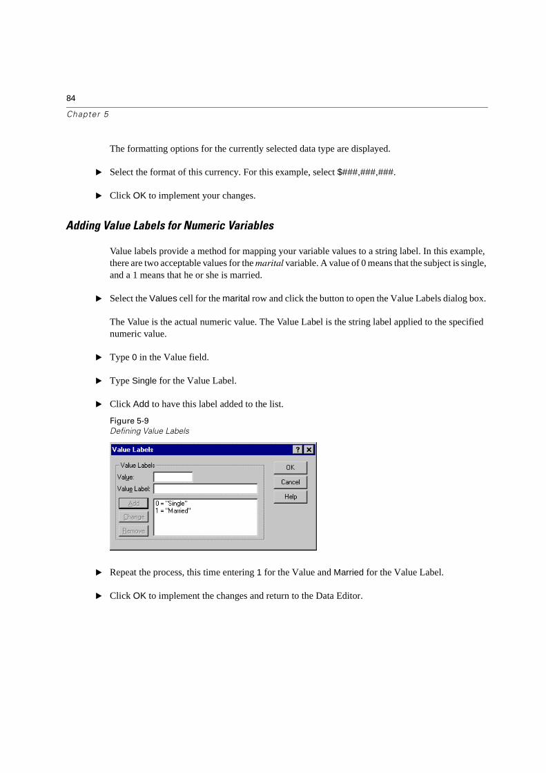
� Select the Values cell for the marital row and click the button to open the Value Labels dialog box.
The Value is the actual numeric value. The Value Label is the string label applied to the specified numeric value.
� Type 0 in the Value field.
� Type Single for the Value Label.
� Click Add to have this label added to the list.
Figure 5-9
Defining Value Labels
� Repeat the process, this time entering 1 for the Value and Married for the Value Label.
� Click OK to implement the changes and return to the Data Editor.
85
Using the Data Editor
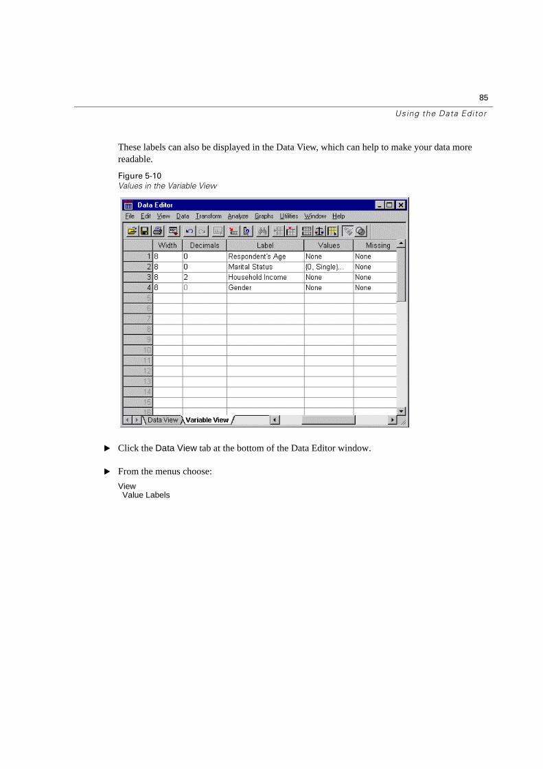
These labels can also be displayed in the Data View, which can help to make your data more readable.
Figure 5-10
Values in the Variable View
� Click the Data View tab at the bottom of the Data Editor window.
� From the menus choose:
ViewValue Labels
86
Chapter 5
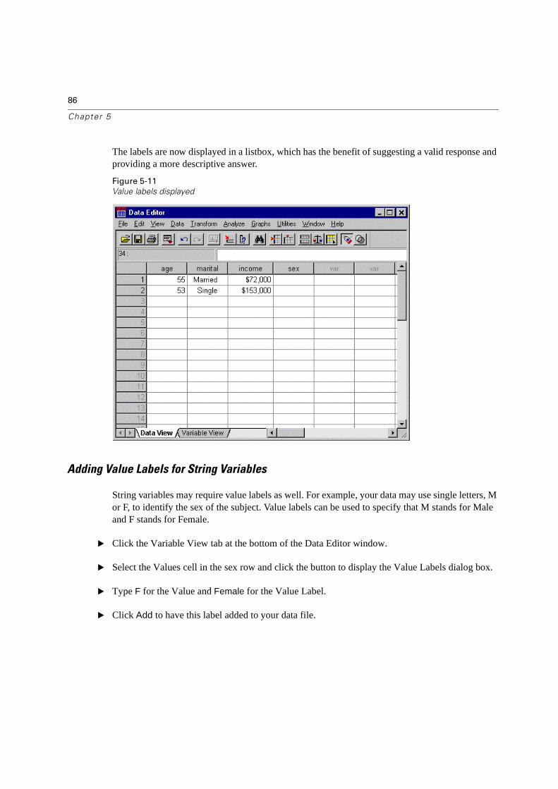
The labels are now displayed in a listbox, which has the benefit of suggesting a valid response and providing a more descriptive answer.
Figure 5-11
Value labels displayed
Adding Value Labels for String Variables
String variables may require value labels as well. For example, your data may use single letters, M or F, to identify the sex of the subject. Value labels can be used to specify that M stands for Male and F stands for Female.
� Click the Variable View tab at the bottom of the Data Editor window.
� Select the Values cell in the sex row and click the button to display the Value Labels dialog box.
� Type F for the Value and Female for the Value Label.
� Click Add to have this label added to your data file.
87
Using the Data Editor
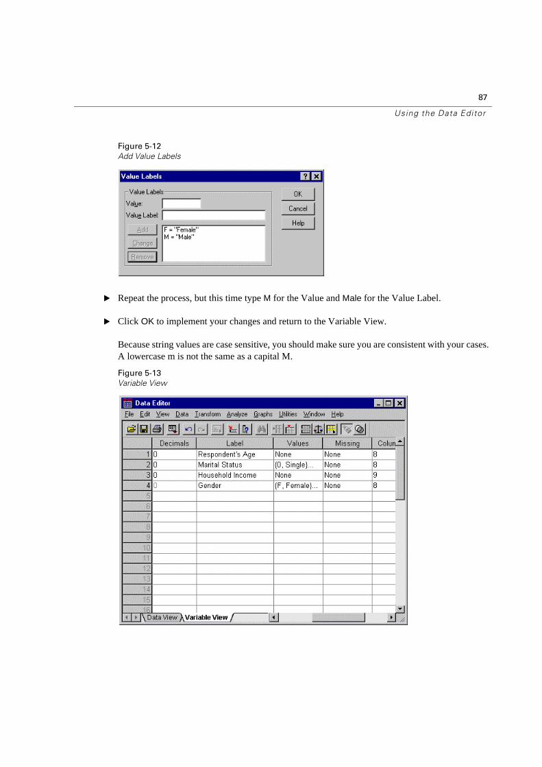
Figure 5-12
Add Value Labels
� Repeat the process, but this time type M for the Value and Male for the Value Label.
� Click OK to implement your changes and return to the Variable View.
Because string values are case sensitive, you should make sure you are consistent with your cases. A lowercase m is not the same as a capital M.
Figure 5-13
Variable View
88
Chapter 5
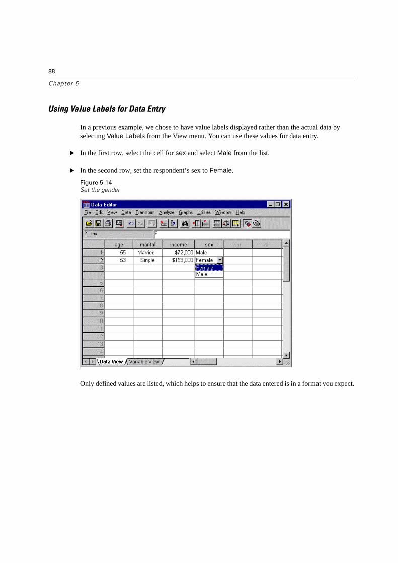
Using Value Labels for Data Entry
In a previous example, we chose to have value labels displayed rather than the actual data by selecting Value Labels from the View menu. You can use these values for data entry.
� In the first row, select the cell for sex and select Male from the list.
� In the second row, set the respondent’s sex to Female.
Figure 5-14
Set the gender
Only defined values are listed, which helps to ensure that the data entered is in a format you expect.
89
Using the Data Editor
Handling Missing Data
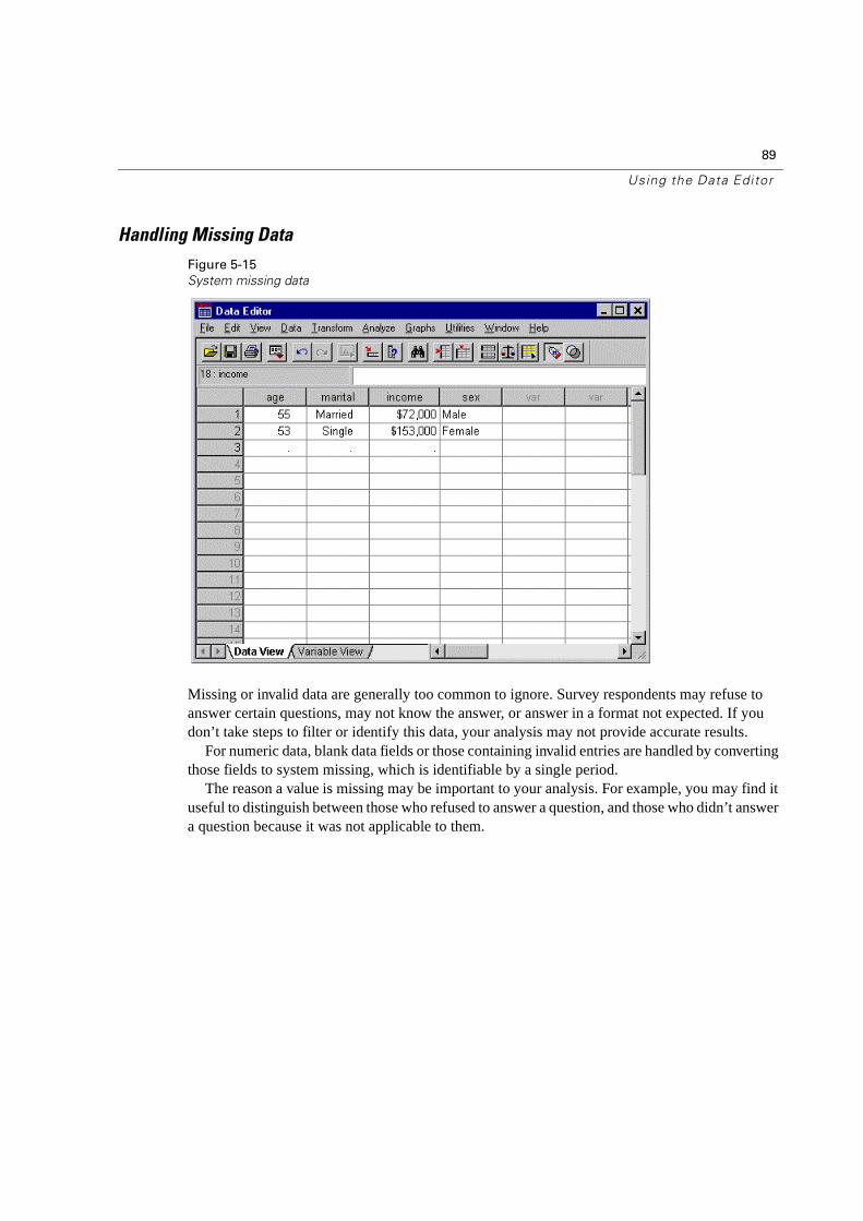
Figure 5-15
System missing data
Missing or invalid data are generally too common to ignore. Survey respondents may refuse to answer certain questions, may not know the answer, or answer in a format not expected. If you don’t take steps to filter or identify this data, your analysis may not provide accurate results.
For numeric data, blank data fields or those containing invalid entries are handled by converting those fields to system missing, which is identifiable by a single period.
The reason a value is missing may be important to your analysis. For example, you may find it useful to distinguish between those who refused to answer a question, and those who didn’t answer a question because it was not applicable to them.
90
Chapter 5
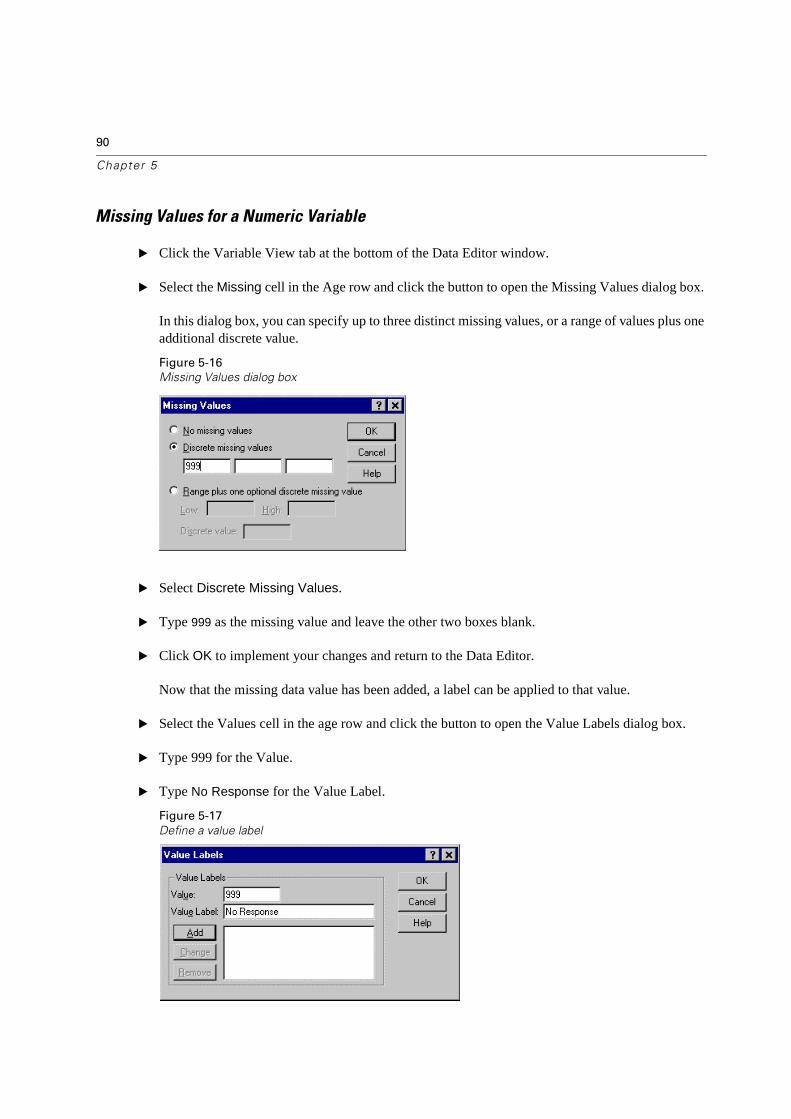
Missing Values for a Numeric Variable
� Click the Variable View tab at the bottom of the Data Editor window.
� Select the Missing cell in the Age row and click the button to open the Missing Values dialog box.
In this dialog box, you can specify up to three distinct missing values, or a range of values plus one additional discrete value.
Figure 5-16
Missing Values dialog box
� Select Discrete Missing Values.
� Type999 as the missing value and leave the other two boxes blank.
� Click OK to implement your changes and return to the Data Editor.
Now that the missing data value has been added, a label can be applied to that value.
� Select the Values cell in the age row and click the button to open the Value Labels dialog box.
� Type 999 for the Value.
� Type No Response for the Value Label.
Figure 5-17
Define a value label
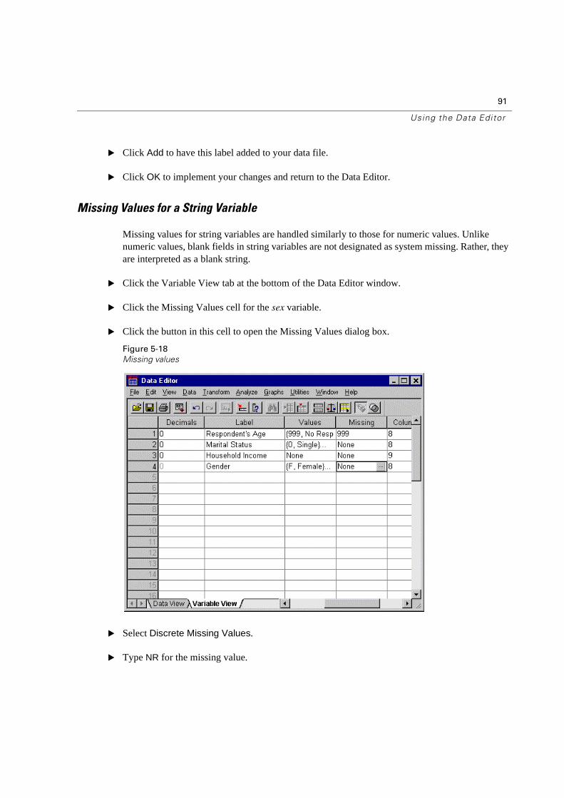
91
Using the Data Editor
� Click Add to have this label added to your data file.
� Click OK to implement your changes and return to the Data Editor.
Missing Values for a String Variable
Missing values for string variables are handled similarly to those for numeric values. Unlike numeric values, blank fields in string variables are not designated as system missing. Rather, they are interpreted as a blank string.
� Click the Variable View tab at the bottom of the Data Editor window.
� Click the Missing Values cell for the sex variable.
� Click the button in this cell to open the Missing Values dialog box.
Figure 5-18
Missing values
� Select Discrete Missing Values.
� Type NR for the missing value.
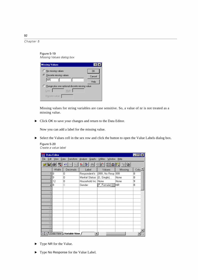
92
Chapter 5
Figure 5-19
Missing Values dialog box
Missing values for string variables are case sensitive. So, a value of nr is not treated as a missing value.
� Click OK to save your changes and return to the Data Editor.
Now you can add a label for the missing value.
� Select the Values cell in the sex row and click the button to open the Value Labels dialog box.
Figure 5-20
Create a value label
� Type NR for the Value.
� Type No Response for the Value Label.
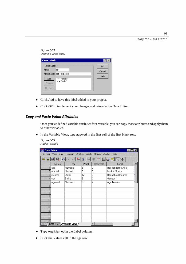
93
Using the Data Editor
Figure 5-21
Define a value label
� Click Add to have this label added to your project.
� Click OK to implement your changes and return to the Data Editor.
Copy and Paste Value Attributes
Once you’ve defined variable attributes for a variable, you can copy those attributes and apply them to other variables.
� In the Variable View, type agewed in the first cell of the first blank row.
Figure 5-22
Add a variable
� Type Age Married in the Label column.
� Click the Values cell in the age row.
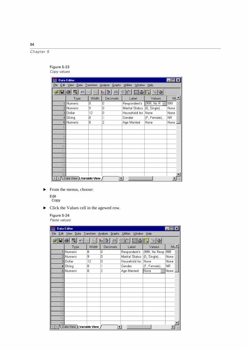
94
Chapter 5
Figure 5-23
Copy values
� From the menus, choose:
EditCopy
� Click the Values cell in the agewed row.
Figure 5-24
Paste values
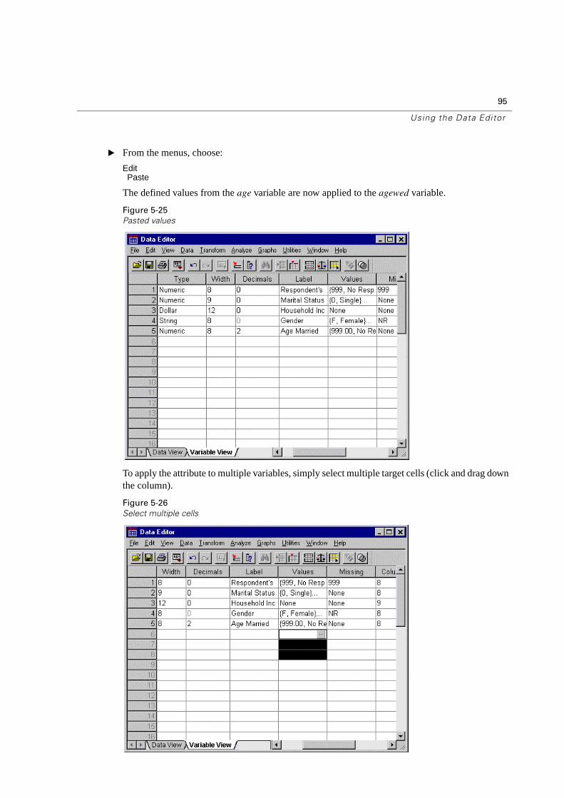
95
Using the Data Editor
� From the menus, choose:
EditPaste
The defined values from the age variable are now applied to the agewed variable.
Figure 5-25
Pasted values
To apply the attribute to multiple variables, simply select multiple target cells (click and drag down the column).
Figure 5-26
Select multiple cells
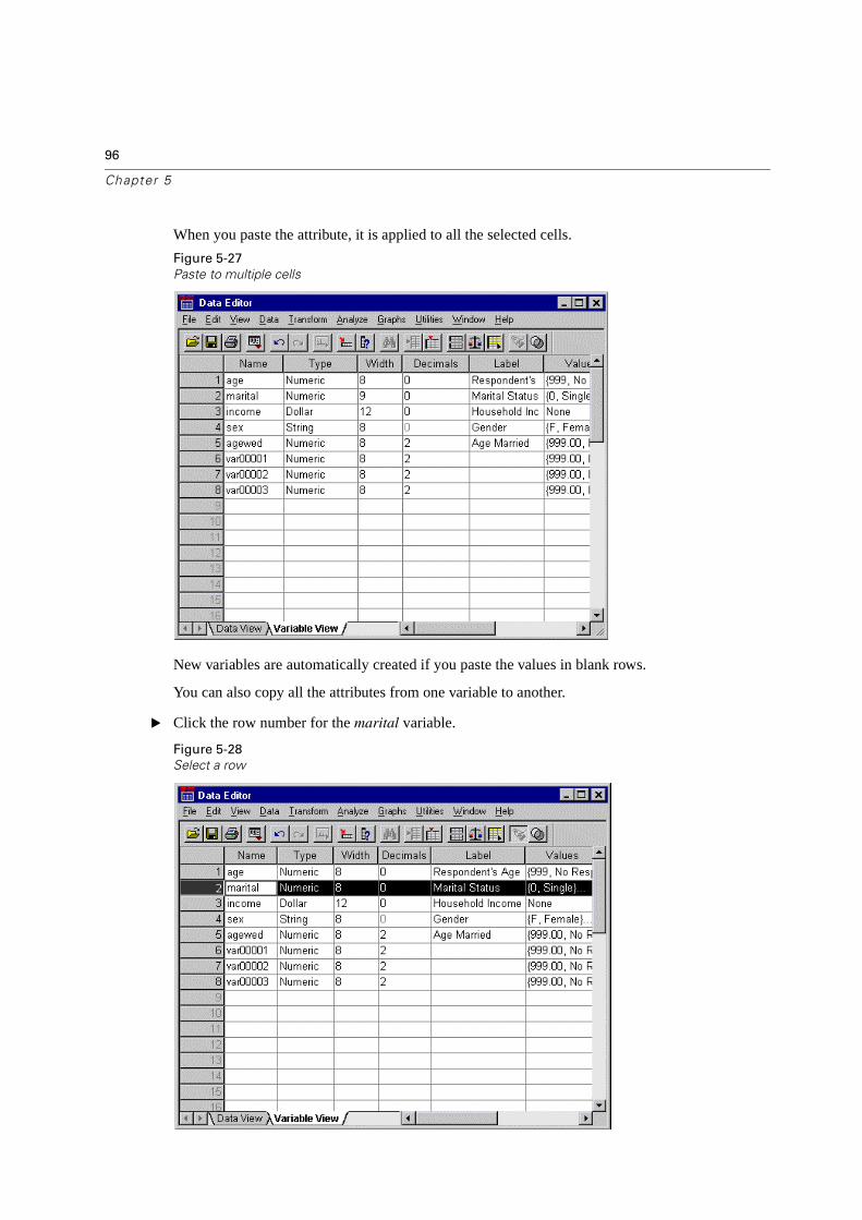
96
Chapter 5
When you paste the attribute, it is applied to all the selected cells.
Figure 5-27
Paste to multiple cells
New variables are automatically created if you paste the values in blank rows.
You can also copy all the attributes from one variable to another.
� Click the row number for the marital variable.
Figure 5-28
Select a row
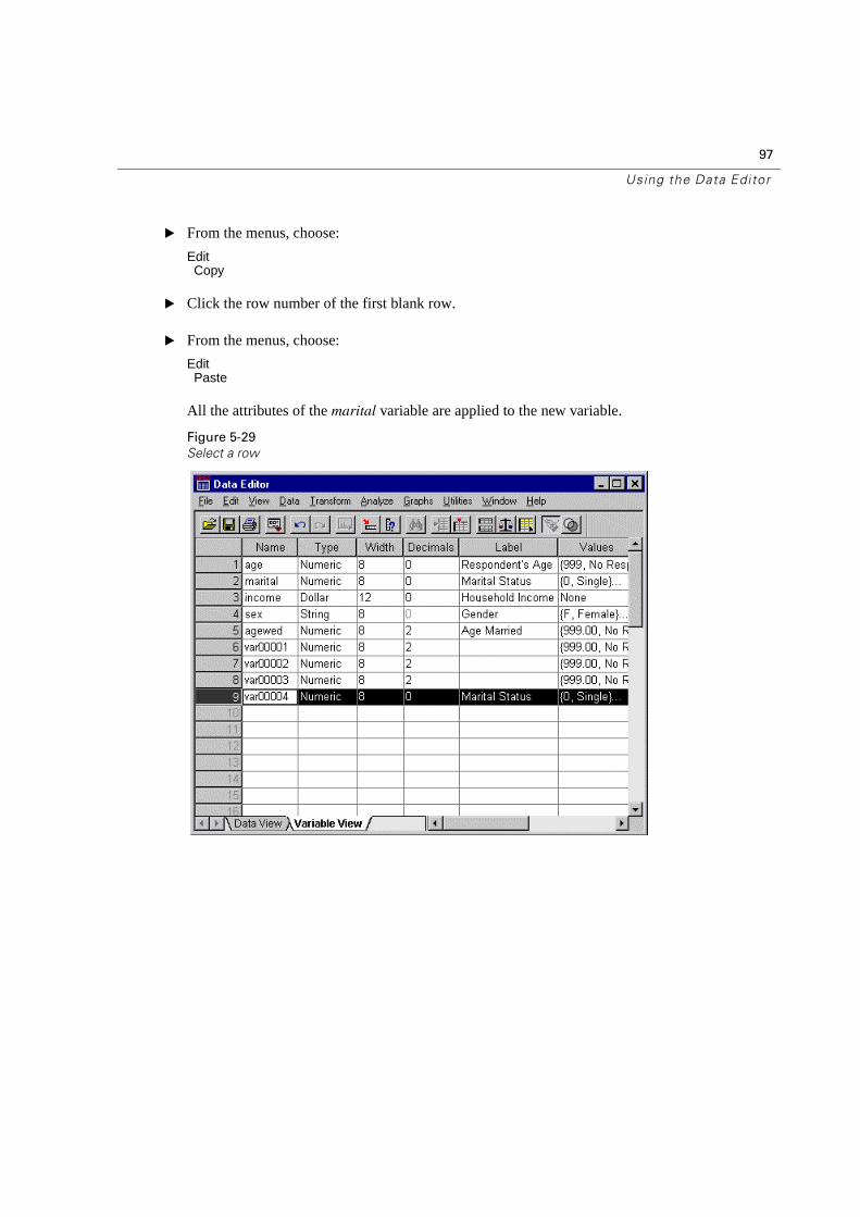
97
Using the Data Editor
� From the menus, choose:
EditCopy
� Click the row number of the first blank row.
� From the menus, choose:
EditPaste
All the attributes of the marital variable are applied to the new variable.
Figure 5-29
Select a row

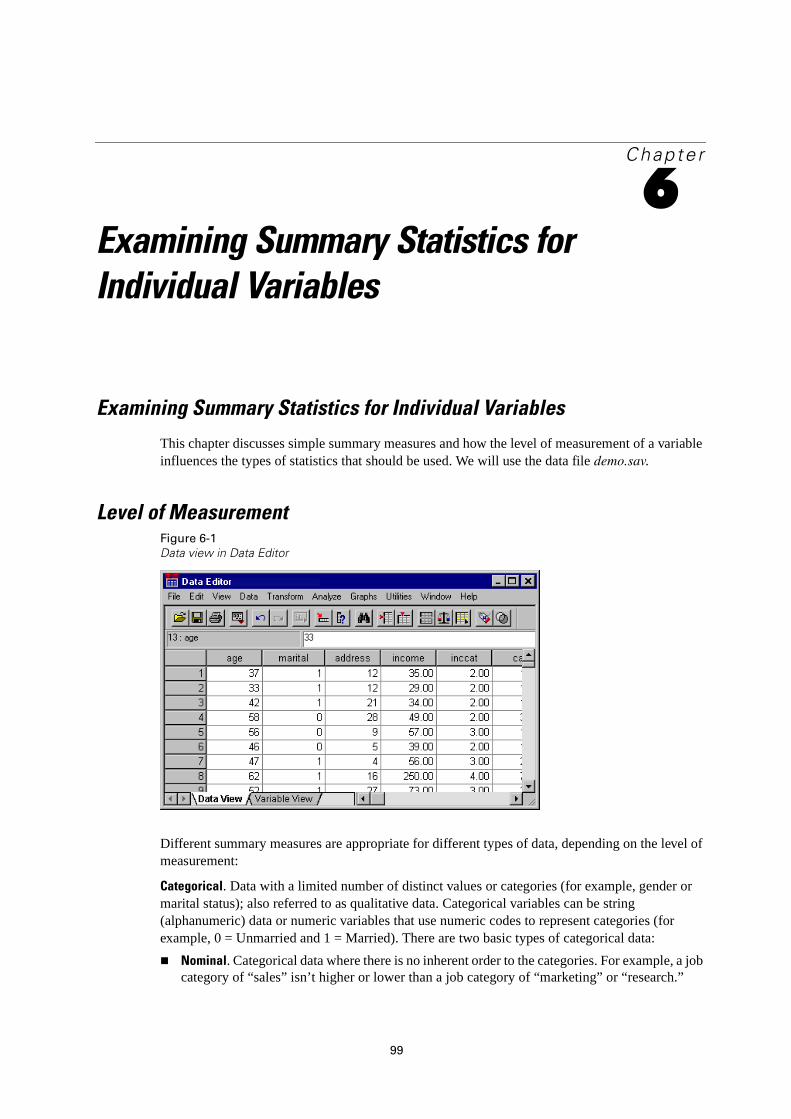
99
Chapte r
6Examining Summary Statistics for
Individual Variables
Examining Summary Statistics for Individual Variables
This chapter discusses simple summary measures and how the level of measurement of a variable influences the types of statistics that should be used. We will use the data file demo.sav.
Level of MeasurementFigure 6-1
Data view in Data Editor
Different summary measures are appropriate for different types of data, depending on the level of measurement:
Categorical. Data with a limited number of distinct values or categories (for example, gender or marital status); also referred to as qualitative data. Categorical variables can be string (alphanumeric) data or numeric variables that use numeric codes to represent categories (for example, 0 = Unmarried and 1 = Married). There are two basic types of categorical data:
� Nominal. Categorical data where there is no inherent order to the categories. For example, a job category of “sales” isn’t higher or lower than a job category of “marketing” or “research.”
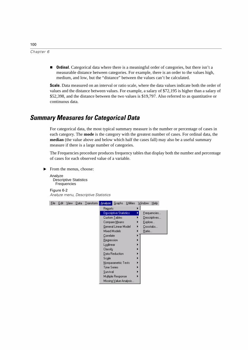
100
Chapter 6
� Ordinal. Categorical data where there is a meaningful order of categories, but there isn’t a measurable distance between categories. For example, there is an order to the values high, medium, and low, but the “distance” between the values can’t be calculated.
Scale. Data measured on an interval or ratio scale, where the data values indicate both the order of values and the distance between values. For example, a salary of $72,195 is higher than a salary of $52,398, and the distance between the two values is $19,797. Also referred to as quantitative or continuous data.
Summary Measures for Categorical Data
For categorical data, the most typical summary measure is the number or percentage of cases in each category. The mode is the category with the greatest number of cases. For ordinal data, the median (the value above and below which half the cases fall) may also be a useful summary measure if there is a large number of categories.
The Frequencies procedure produces frequency tables that display both the number and percentage of cases for each observed value of a variable.
� From the menus, choose:
Analyze Descriptive Statistics
Frequencies
Figure 6-2
Analyze menu, Descriptive Statistics
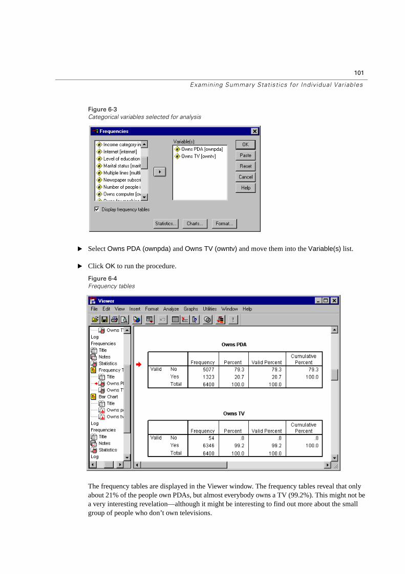
101
Examining Summary Stat istics for Individual Variables
Figure 6-3
Categorical variables selected for analysis
� Select Owns PDA (ownpda) andOwns TV (owntv) and move them into the Variable(s) list.
� Click OK to run the procedure.
Figure 6-4
Frequency tables
The frequency tables are displayed in the Viewer window. The frequency tables reveal that only about 21% of the people own PDAs, but almost everybody owns a TV (99.2%). This might not be a very interesting revelation—although it might be interesting to find out more about the small group of people who don’t own televisions.
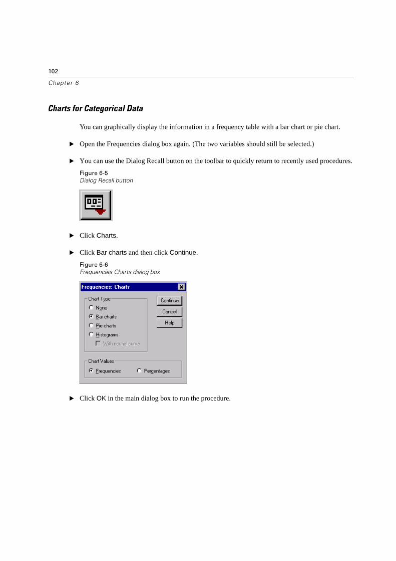
102
Chapter 6
Charts for Categorical Data
You can graphically display the information in a frequency table with a bar chart or pie chart.
� Open the Frequencies dialog box again. (The two variables should still be selected.)
� You can use the Dialog Recall button on the toolbar to quickly return to recently used procedures.
Figure 6-5
Dialog Recall button
� Click Charts.
� Click Bar charts and then click Continue.
Figure 6-6
Frequencies Charts dialog box
� Click OK in the main dialog box to run the procedure.
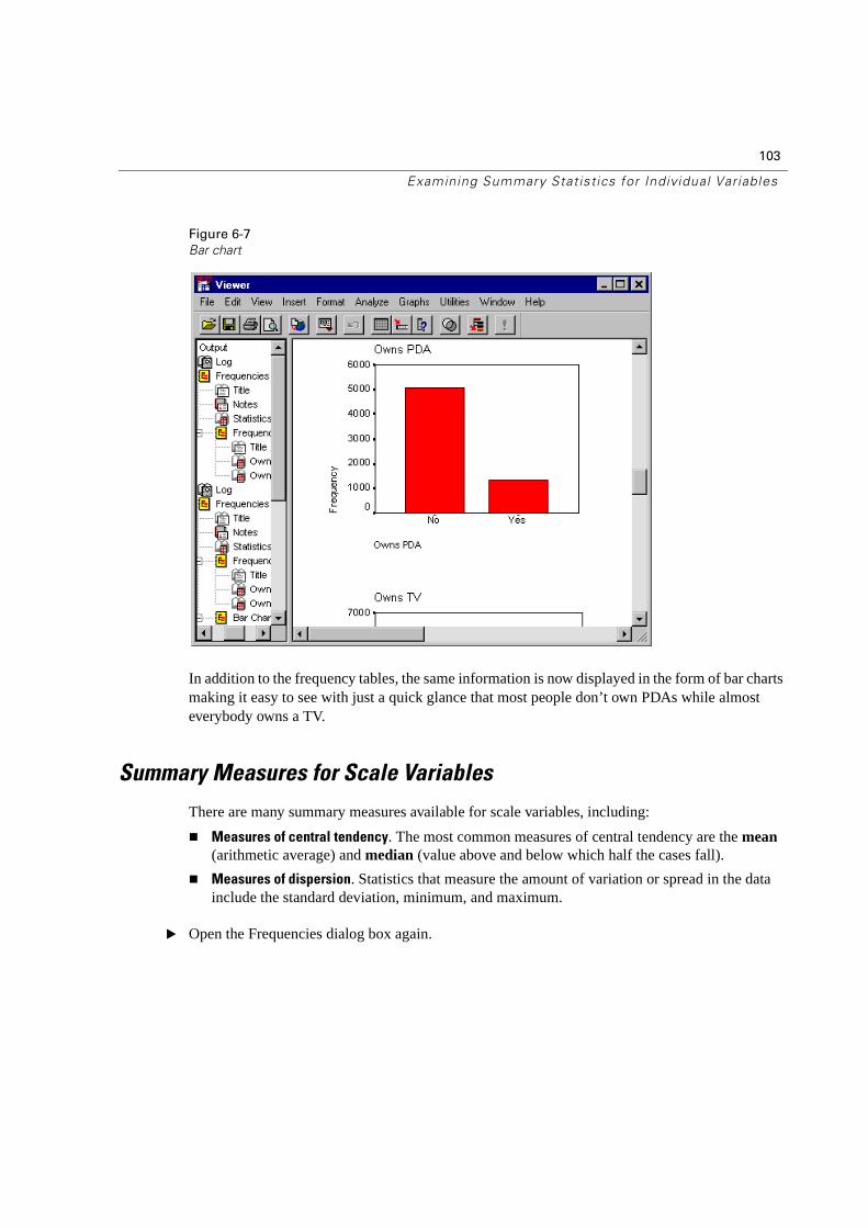
103
Examining Summary Stat istics for Individual Variables
Figure 6-7
Bar chart
In addition to the frequency tables, the same information is now displayed in the form of bar charts making it easy to see with just a quick glance that most people don’t own PDAs while almost everybody owns a TV.
Summary Measures for Scale Variables
There are many summary measures available for scale variables, including:
� Measures of central tendency. The most common measures of central tendency are the mean(arithmetic average) and median (value above and below which half the cases fall).
� Measures of dispersion. Statistics that measure the amount of variation or spread in the data include the standard deviation, minimum, and maximum.
� Open the Frequencies dialog box again.
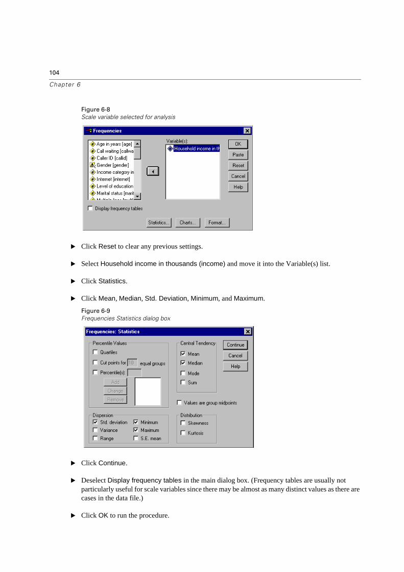
104
Chapter 6
Figure 6-8
Scale variable selected for analysis
� Click Reset to clear any previous settings.
� Select Household income in thousands (income) and move it into the Variable(s) list.
� Click Statistics.
� Click Mean, Median, Std. Deviation, Minimum, and Maximum.
Figure 6-9
Frequencies Statistics dialog box
� Click Continue.
� Deselect Display frequency tables in the main dialog box. (Frequency tables are usually not particularly useful for scale variables since there may be almost as many distinct values as there are cases in the data file.)
� Click OK to run the procedure.
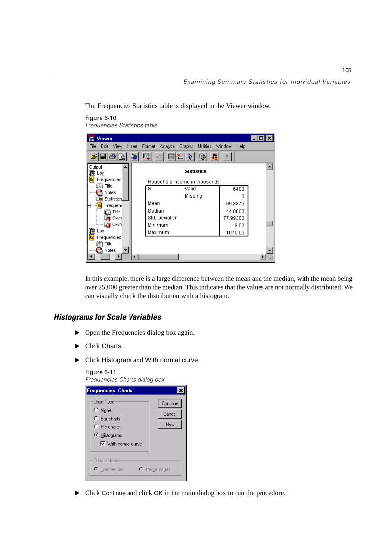
105
Examining Summary Stat istics for Individual Variables
The Frequencies Statistics table is displayed in the Viewer window.
Figure 6-10
Frequencies Statistics table
In this example, there is a large difference between the mean and the median, with the mean being over 25,000 greater than the median. This indicates that the values are not normally distributed. We can visually check the distribution with a histogram.
Histograms for Scale Variables
� Open the Frequencies dialog box again.
� Click Charts.
� Click Histogram and With normal curve.
Figure 6-11
Frequencies Charts dialog box
� Click Continue and click OK in the main dialog box to run the procedure.
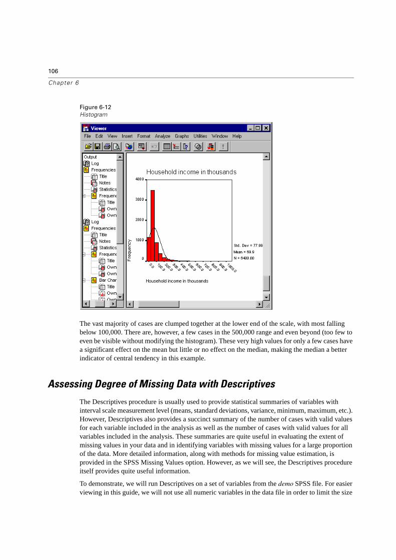
106
Chapter 6
Figure 6-12
Histogram
The vast majority of cases are clumped together at the lower end of the scale, with most falling below 100,000. There are, however, a few cases in the 500,000 range and even beyond (too few to even be visible without modifying the histogram). These very high values for only a few cases have a significant effect on the mean but little or no effect on the median, making the median a better indicator of central tendency in this example.
Assessing Degree of Missing Data with Descriptives
The Descriptives procedure is usually used to provide statistical summaries of variables with interval scale measurement level (means, standard deviations, variance, minimum, maximum, etc.). However, Descriptives also provides a succinct summary of the number of cases with valid values for each variable included in the analysis as well as the number of cases with valid values for all variables included in the analysis. These summaries are quite useful in evaluating the extent of missing values in your data and in identifying variables with missing values for a large proportion of the data. More detailed information, along with methods for missing value estimation, is provided in the SPSS Missing Values option. However, as we will see, the Descriptives procedure itself provides quite useful information.
To demonstrate, we will run Descriptives on a set of variables from the demo SPSS file. For easier viewing in this guide, we will not use all numeric variables in the data file in order to limit the size
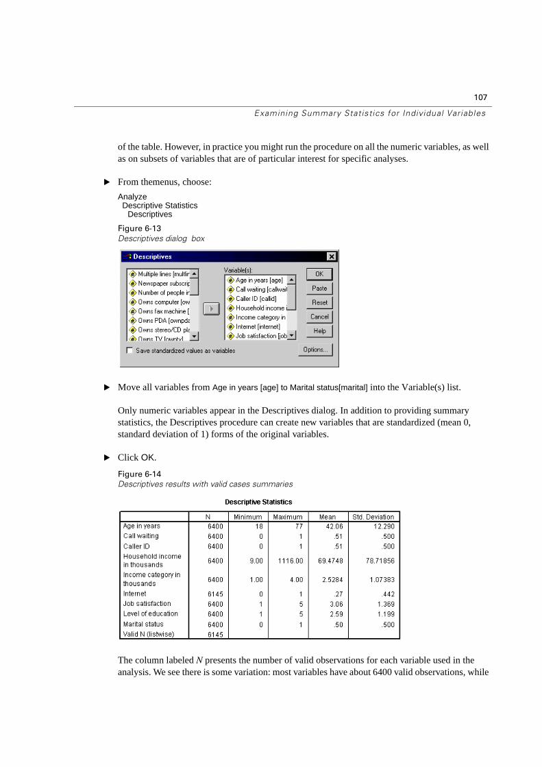
107
Examining Summary Stat istics for Individual Variables
of the table. However, in practice you might run the procedure on all the numeric variables, as well as on subsets of variables that are of particular interest for specific analyses.
� From themenus, choose:
AnalyzeDescriptive Statistics
Descriptives
Figure 6-13
Descriptives dialog box
� Move all variables from Age in years [age] to Marital status[marital] into the Variable(s) list.
Only numeric variables appear in the Descriptives dialog. In addition to providing summary statistics, the Descriptives procedure can create new variables that are standardized (mean 0, standard deviation of 1) forms of the original variables.
� Click OK.
Figure 6-14
Descriptives results with valid cases summaries
The column labeled N presents the number of valid observations for each variable used in the analysis. We see there is some variation: most variables have about 6400 valid observations, while

108
Chapter 6
Internet (respondent has an internet connection) has only 6145 valid observations. This information would be helpful in evaluating which variables could be used in analyses.
The value in the N column for the last row in the table (labeled Valid N (listwise)) indicates how many cases contain valid values for all variables appearing in the table. Here 6145 do, entirely because of the smaller N values for Internet. If you were performing analyses requiring no missing information for variables, then it is helpful to know how many cases have complete information and which variables are likely to be the main sources of the problem. Although it isn’t the focus of this analysis, we see that minimum, maximum, mean, and standard deviations, display by default.
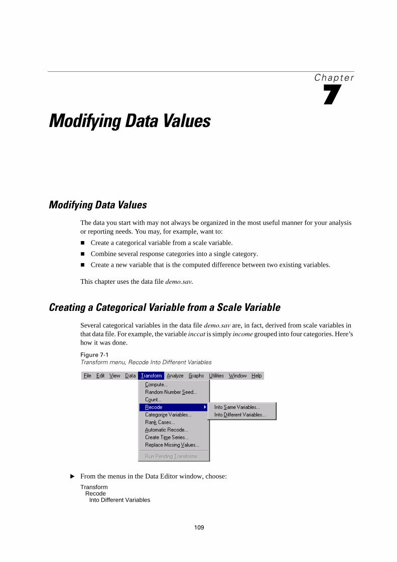
109
Chapte r
7Modifying Data Values
Modifying Data Values
The data you start with may not always be organized in the most useful manner for your analysis or reporting needs. You may, for example, want to:
� Create a categorical variable from a scale variable.
� Combine several response categories into a single category.
� Create a new variable that is the computed difference between two existing variables.
This chapter uses the data file demo.sav.
Creating a Categorical Variable from a Scale Variable
Several categorical variables in the data file demo.sav are, in fact, derived from scale variables in that data file. For example, the variable inccat is simply income grouped into four categories. Here’show it was done.
Figure 7-1
Transform menu, Recode Into Different Variables
� From the menus in the Data Editor window, choose:
Transform Recode
Into Different Variables
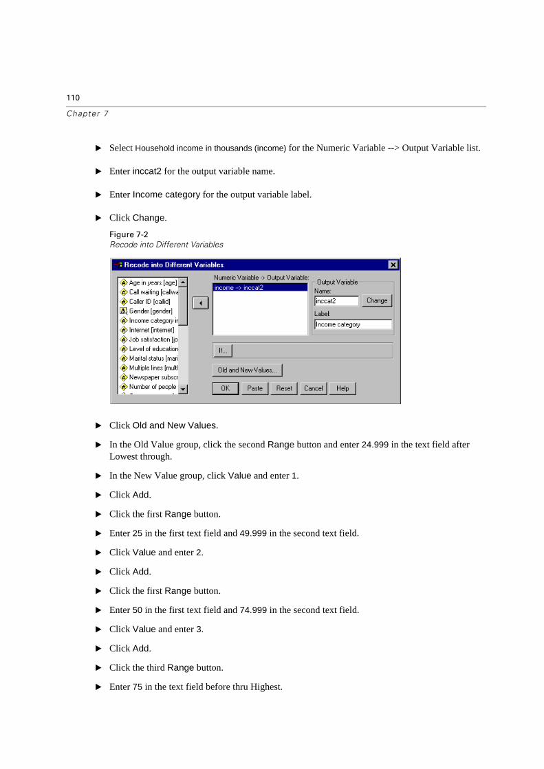
110
Chapter 7
� Select Household income in thousands (income) for the Numeric Variable --> Output Variable list.
� Enter inccat2 for the output variable name.
� Enter Income category for the output variable label.
� Click Change.
Figure 7-2
Recode into Different Variables
� Click Old and New Values.
� In the Old Value group, click the second Range button and enter 24.999 in the text field after Lowest through.
� In the New Value group, click Value and enter 1.
� Click Add.
� Click the first Range button.
� Enter 25 in the first text field and 49.999 in the second text field.
� Click Value and enter 2.
� Click Add.
� Click the first Range button.
� Enter 50 in the first text field and 74.999 in the second text field.
� Click Value and enter 3.
� Click Add.
� Click the third Range button.
� Enter 75 in the text field before thru Highest.
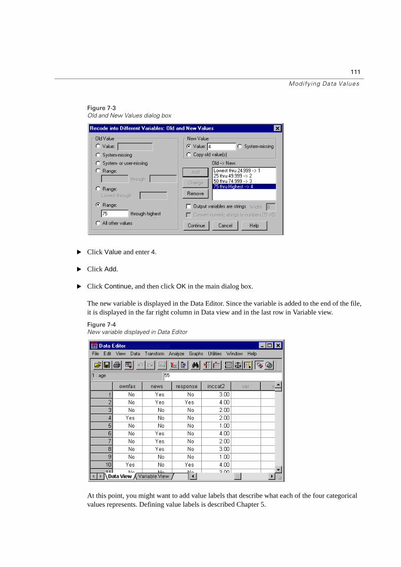
111
Modify ing Data Values
Figure 7-3
Old and New Values dialog box
� Click Value and enter 4.
� Click Add.
� Click Continue, and then click OK in the main dialog box.
The new variable is displayed in the Data Editor. Since the variable is added to the end of the file, it is displayed in the far right column in Data view and in the last row in Variable view.
Figure 7-4
New variable displayed in Data Editor
At this point, you might want to add value labels that describe what each of the four categorical values represents. Defining value labels is described Chapter 5.
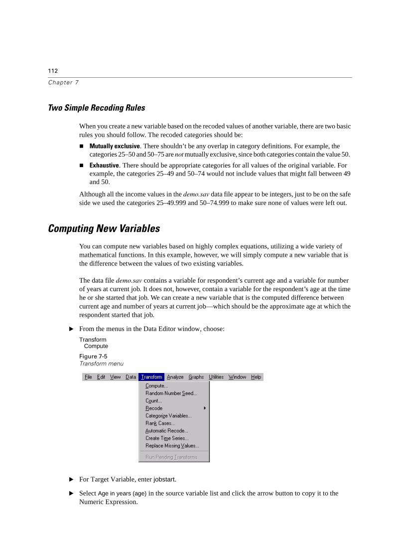
112
Chapter 7
Two Simple Recoding Rules
When you create a new variable based on the recoded values of another variable, there are two basic rules you should follow. The recoded categories should be:
� Mutually exclusive. There shouldn’t be any overlap in category definitions. For example, the categories 25–50 and 50–75 are not mutually exclusive, since both categories contain the value 50.
� Exhaustive. There should be appropriate categories for all values of the original variable. For example, the categories 25–49 and 50–74 would not include values that might fall between 49 and 50.
Although all the income values in the demo.sav data file appear to be integers, just to be on the safe side we used the categories 25–49.999 and 50–74.999 to make sure none of values were left out.
Computing New Variables
You can compute new variables based on highly complex equations, utilizing a wide variety of mathematical functions. In this example, however, we will simply compute a new variable that is the difference between the values of two existing variables.
The data file demo.sav contains a variable for respondent’s current age and a variable for number of years at current job. It does not, however, contain a variable for the respondent’s age at the time he or she started that job. We can create a new variable that is the computed difference between current age and number of years at current job—which should be the approximate age at which the respondent started that job.
� From the menus in the Data Editor window, choose:
Transform Compute
Figure 7-5
Transform menu
� For Target Variable, enter jobstart.
� Select Age in years (age) in the source variable list and click the arrow button to copy it to the Numeric Expression.
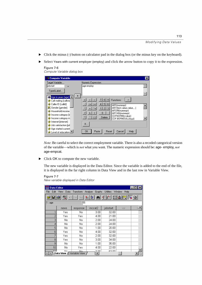
113
Modify ing Data Values
� Click the minus (-) button on calculator pad in the dialog box (or the minus key on the keyboard).
� Select Years with current employer (employ) and click the arrow button to copy it to the expression.
Figure 7-6
Compute Variable dialog box
Note: Be careful to select the correct employment variable. There is also a recoded categorical version of the variable—which is not what you want. The numeric expression should be: age- employ, not
age-empcat.
� Click OK to compute the new variable.
The new variable is displayed in the Data Editor. Since the variable is added to the end of the file, it is displayed in the far right column in Data View and in the last row in Variable View.
Figure 7-7
New variable displayed in Data Editor
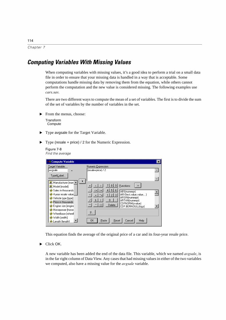
114
Chapter 7
Computing Variables With Missing Values
When computing variables with missing values, it’s a good idea to perform a trial on a small data file in order to ensure that your missing data is handled in a way that is acceptable. Some computations handle missing data by removing them from the equation, while others cannot perform the computation and the new value is considered missing. The following examples use cars.sav.
There are two different ways to compute the mean of a set of variables. The first is to divide the sum of the set of variables by the number of variables in the set.
� From the menus, choose:
TransformCompute
� Type avgsale for the Target Variable.
� Type (resale + price) / 2 for the Numeric Expression.
Figure 7-8
Find the average
This equation finds the average of the original price of a car and its four-year resale price.
� Click OK.
A new variable has been added the end of the data file. This variable, which we named avgsale, is in the far right column of Data View. Any cases that had missing values in either of the two variables we computed, also have a missing value for the avgsale variable.
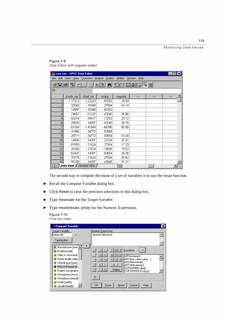
115
Modify ing Data Values
Figure 7-9
Data Editor with avgsale added
The second way to compute the mean of a set of variables is to use the mean function.
� Recall the Compute Variable dialog box.
� Click Reset to clear the previous selections in this dialog box.
� Type meansale for the Target Variable.
� Type mean(resale, price) for the Numeric Expression.
Figure 7-10
Find the mean
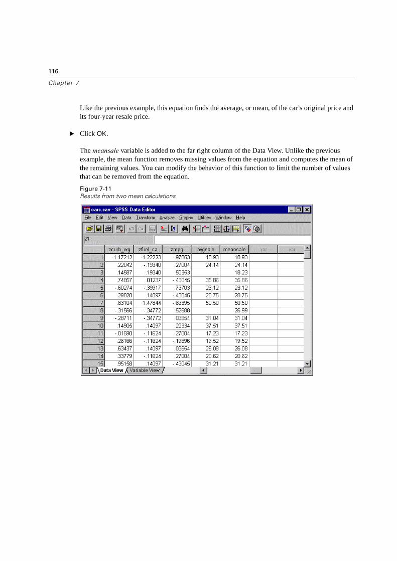
116
Chapter 7
Like the previous example, this equation finds the average, or mean, of the car’s original price and its four-year resale price.
� Click OK.
The meansale variable is added to the far right column of the Data View. Unlike the previous example, the mean function removes missing values from the equation and computes the mean of the remaining values. You can modify the behavior of this function to limit the number of values that can be removed from the equation.
Figure 7-11
Results from two mean calculations
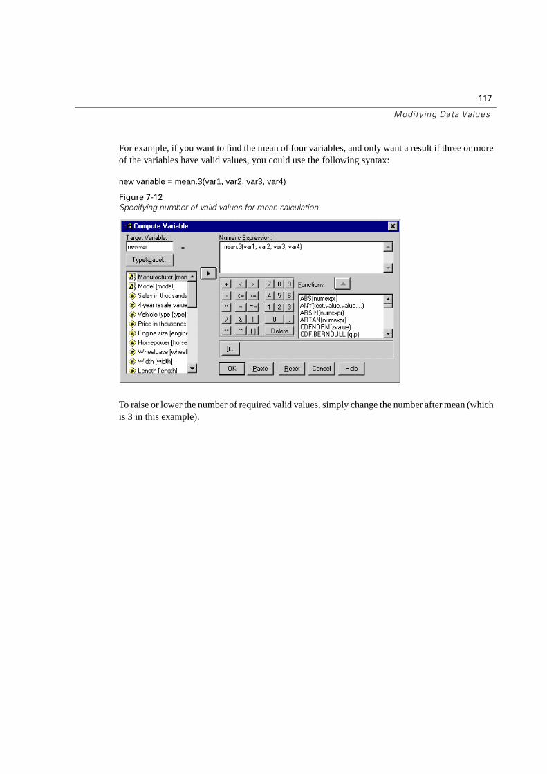
117
Modify ing Data Values
For example, if you want to find the mean of four variables, and only want a result if three or more of the variables have valid values, you could use the following syntax:
new variable = mean.3(var1, var2, var3, var4)
Figure 7-12
Specifying number of valid values for mean calculation
To raise or lower the number of required valid values, simply change the number after mean (which is 3 in this example).

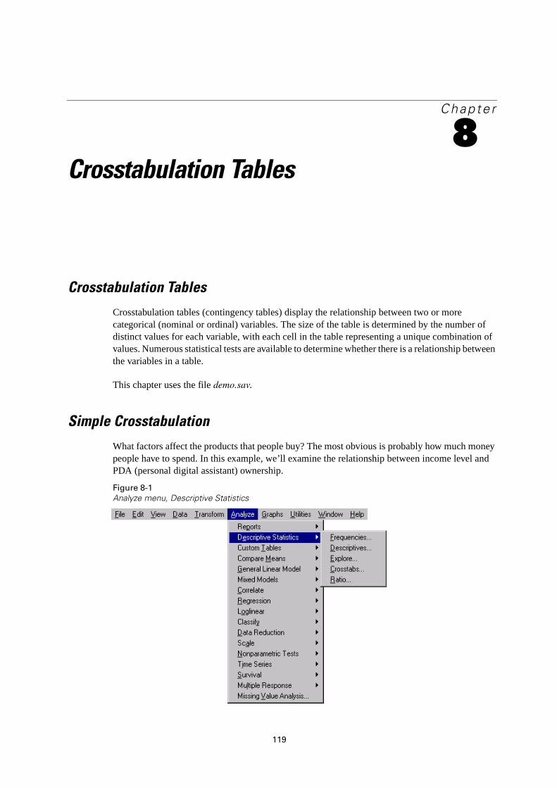
119
Chapte r
8Crosstabulation Tables
Crosstabulation Tables
Crosstabulation tables (contingency tables) display the relationship between two or more categorical (nominal or ordinal) variables. The size of the table is determined by the number of distinct values for each variable, with each cell in the table representing a unique combination of values. Numerous statistical tests are available to determine whether there is a relationship between the variables in a table.
This chapter uses the file demo.sav.
Simple Crosstabulation
What factors affect the products that people buy? The most obvious is probably how much money people have to spend. In this example, we’ll examine the relationship between income level and PDA (personal digital assistant) ownership.
Figure 8-1
Analyze menu, Descriptive Statistics
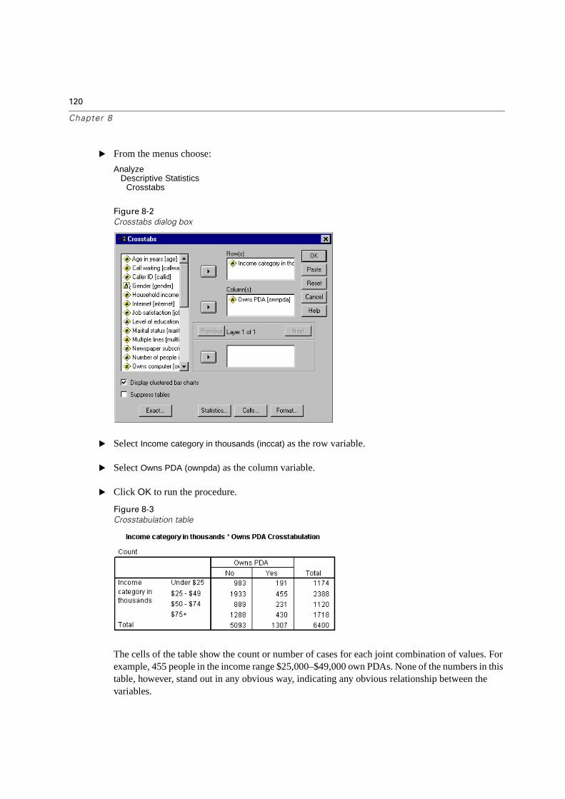
120
Chapter 8
� From the menus choose:
Analyze Descriptive Statistics
Crosstabs
Figure 8-2
Crosstabs dialog box
� Select Income category in thousands (inccat) as the row variable.
� Select Owns PDA (ownpda) as the column variable.
� Click OK to run the procedure.
Figure 8-3
Crosstabulation table
The cells of the table show the count or number of cases for each joint combination of values. For example, 455 people in the income range $25,000–$49,000 own PDAs. None of the numbers in this table, however, stand out in any obvious way, indicating any obvious relationship between the variables.
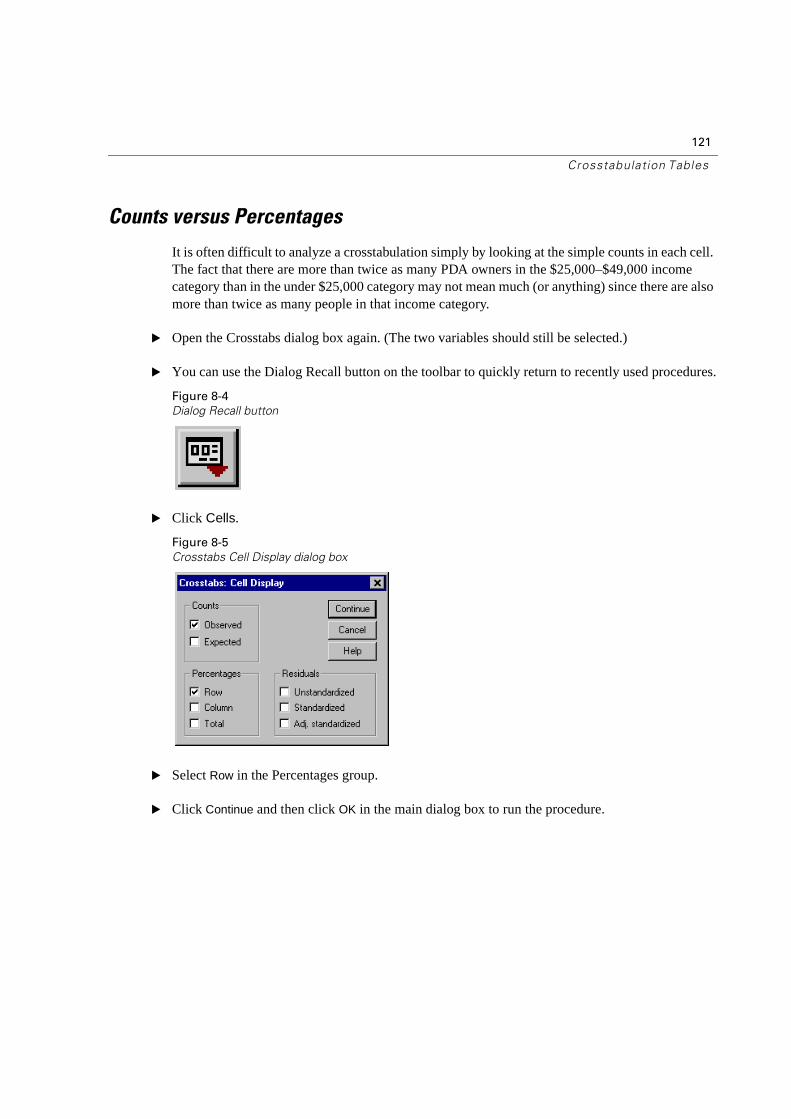
121
Crosstabulation Tables
Counts versus Percentages
It is often difficult to analyze a crosstabulation simply by looking at the simple counts in each cell. The fact that there are more than twice as many PDA owners in the $25,000–$49,000 income category than in the under $25,000 category may not mean much (or anything) since there are also more than twice as many people in that income category.
� Open the Crosstabs dialog box again. (The two variables should still be selected.)
� You can use the Dialog Recall button on the toolbar to quickly return to recently used procedures.
Figure 8-4
Dialog Recall button
� Click Cells.
Figure 8-5
Crosstabs Cell Display dialog box
� Select Row in the Percentages group.
� Click Continue and then click OK in the main dialog box to run the procedure.
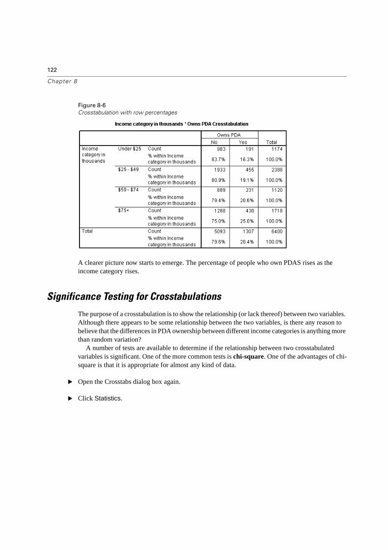
122
Chapter 8
Figure 8-6
Crosstabulation with row percentages
A clearer picture now starts to emerge. The percentage of people who own PDAS rises as the income category rises.
Significance Testing for Crosstabulations
The purpose of a crosstabulation is to show the relationship (or lack thereof) between two variables. Although there appears to be some relationship between the two variables, is there any reason to believe that the differences in PDA ownership between different income categories is anything more than random variation?
A number of tests are available to determine if the relationship between two crosstabulated variables is significant. One of the more common tests is chi-square. One of the advantages of chi-square is that it is appropriate for almost any kind of data.
� Open the Crosstabs dialog box again.
� Click Statistics.
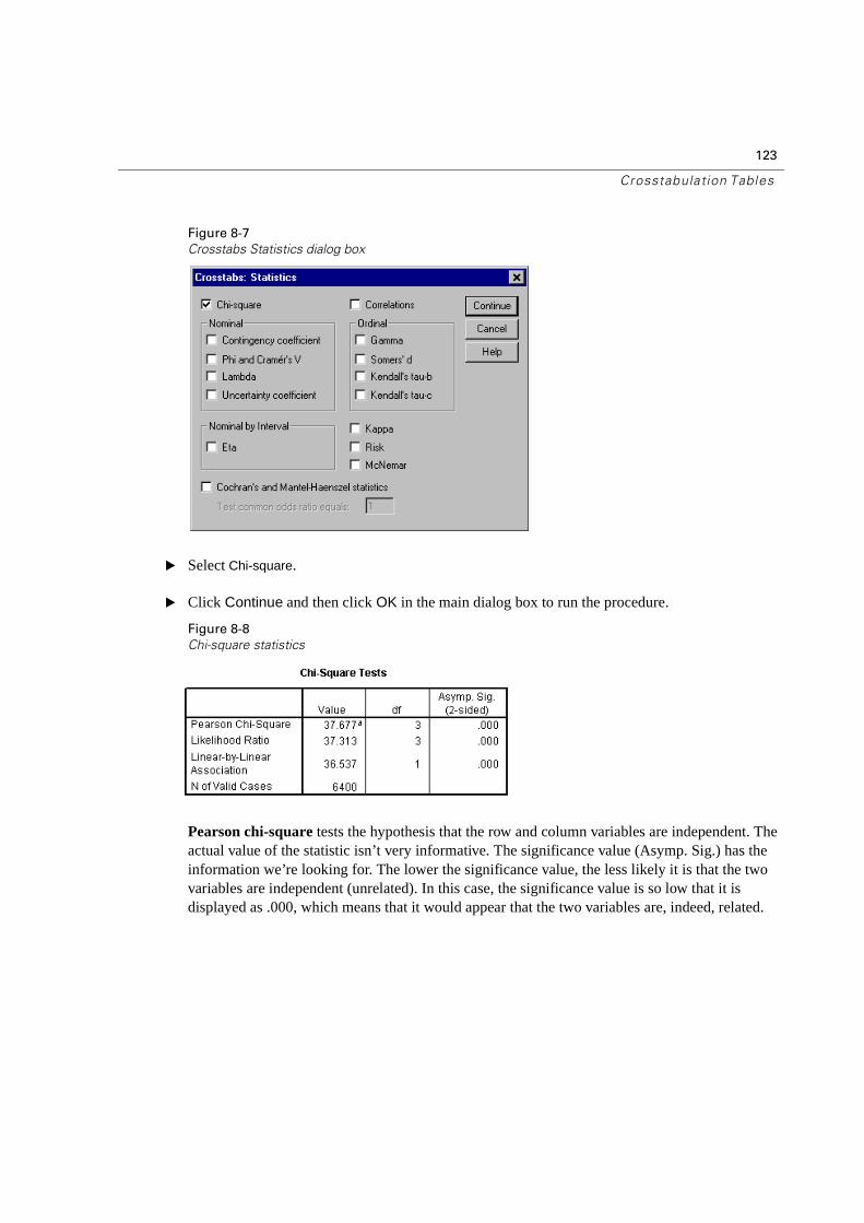
123
Crosstabulation Tables
Figure 8-7
Crosstabs Statistics dialog box
� Select Chi-square.
� Click Continue and then click OK in the main dialog box to run the procedure.
Figure 8-8
Chi-square statistics
Pearson chi-square tests the hypothesis that the row and column variables are independent. The actual value of the statistic isn’t very informative. The significance value (Asymp. Sig.) has the information we’re looking for. The lower the significance value, the less likely it is that the two variables are independent (unrelated). In this case, the significance value is so low that it is displayed as .000, which means that it would appear that the two variables are, indeed, related.
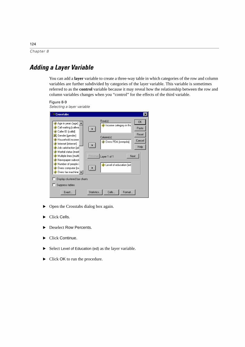
124
Chapter 8
Adding a Layer Variable
You can add a layer variable to create a three-way table in which categories of the row and column variables are further subdivided by categories of the layer variable. This variable is sometimes referred to as the control variable because it may reveal how the relationship between the row and column variables changes when you “control” for the effects of the third variable.
Figure 8-9
Selecting a layer variable
� Open the Crosstabs dialog box again.
� Click Cells.
� Deselect Row Percents.
� Click Continue.
� Select Level of Education (ed) as the layer variable.
� Click OK to run the procedure.
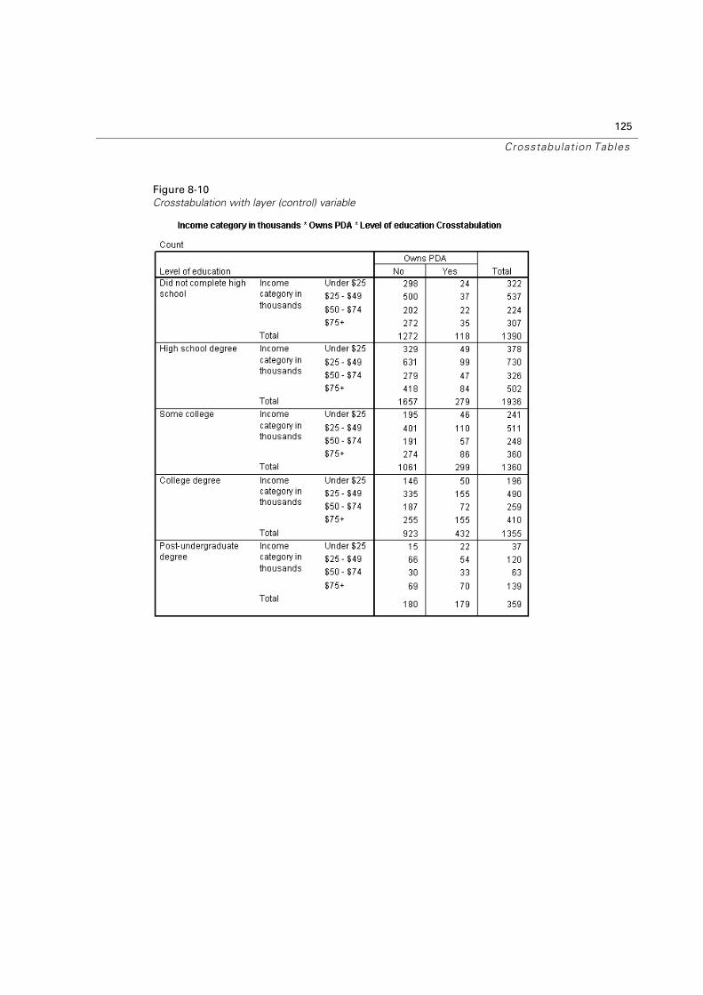
125
Crosstabulation Tables
Figure 8-10
Crosstabulation with layer (control) variable
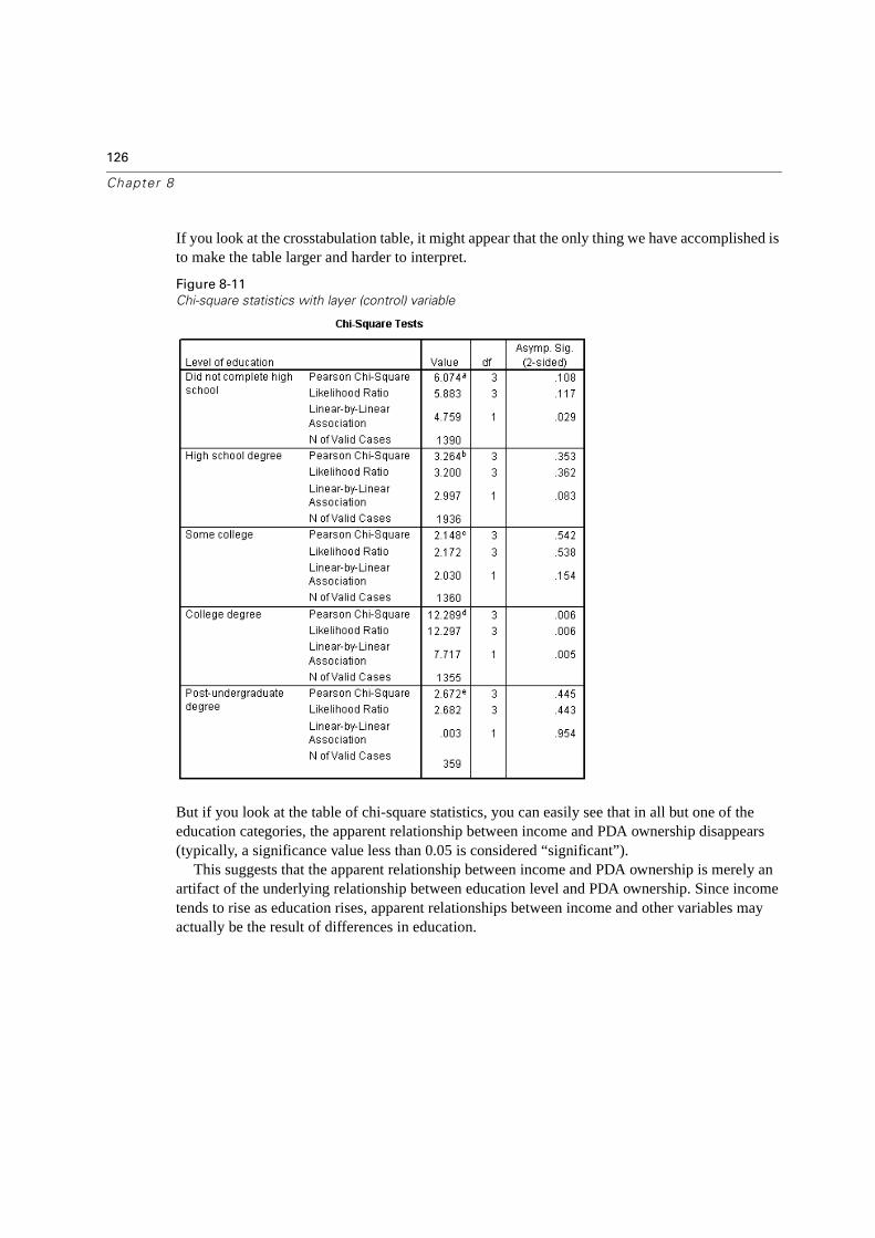
126
Chapter 8
If you look at the crosstabulation table, it might appear that the only thing we have accomplished is to make the table larger and harder to interpret.
Figure 8-11
Chi-square statistics with layer (control) variable
But if you look at the table of chi-square statistics, you can easily see that in all but one of the education categories, the apparent relationship between income and PDA ownership disappears (typically, a significance value less than 0.05 is considered “significant”).
This suggests that the apparent relationship between income and PDA ownership is merely an artifact of the underlying relationship between education level and PDA ownership. Since income tends to rise as education rises, apparent relationships between income and other variables may actually be the result of differences in education.
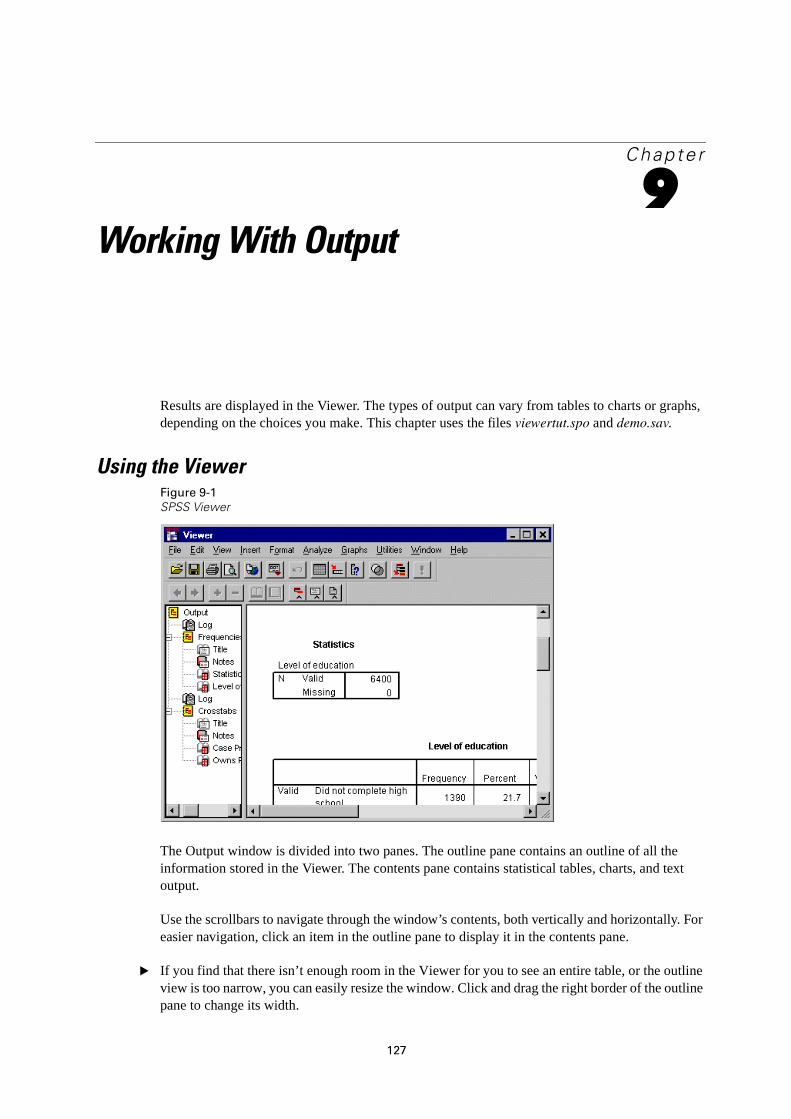
127
Chapte r
9Working With Output
Results are displayed in the Viewer. The types of output can vary from tables to charts or graphs, depending on the choices you make. This chapter uses the files viewertut.spo and demo.sav.
Using the ViewerFigure 9-1
SPSS Viewer
The Output window is divided into two panes. The outline pane contains an outline of all the information stored in the Viewer. The contents pane contains statistical tables, charts, and text output.
Use the scrollbars to navigate through the window’s contents, both vertically and horizontally. For easier navigation, click an item in the outline pane to display it in the contents pane.
� If you find that there isn’t enough room in the Viewer for you to see an entire table, or the outline view is too narrow, you can easily resize the window. Click and drag the right border of the outline pane to change its width.
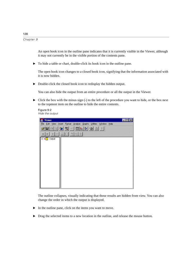
128
Chapter 9
An open book icon in the outline pane indicates that it is currently visible in the Viewer, although it may not currently be in the visible portion of the contents pane.
� To hide a table or chart, double-click its book icon in the outline pane.
The open book icon changes to a closed book icon, signifying that the information associated with it is now hidden.
� Double-click the closed book icon to redisplay the hidden output.
You can also hide the output from an entire procedure or all the output in the Viewer.
� Click the box with the minus sign (-) to the left of the procedure you want to hide, or the box next to the topmost item on the outline to hide the entire contents.
Figure 9-2
Hide the output
The outline collapses, visually indicating that those results are hidden from view. You can also change the order in which the output is displayed.
� In the outline pane, click on the items you want to move.
� Drag the selected items to a new location in the outline, and release the mouse button.
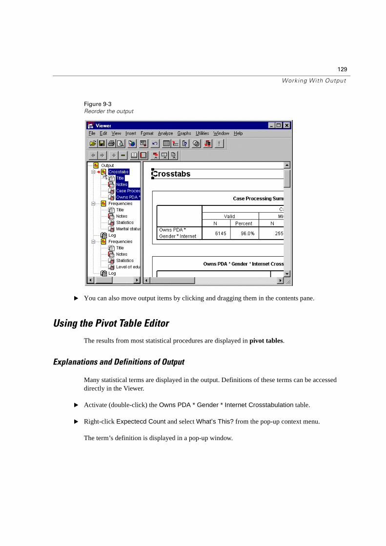
129
Working With Output
Figure 9-3
Reorder the output
� You can also move output items by clicking and dragging them in the contents pane.
Using the Pivot Table Editor
The results from most statistical procedures are displayed in pivot tables.
Explanations and Definitions of Output
Many statistical terms are displayed in the output. Definitions of these terms can be accessed directly in the Viewer.
� Activate (double-click) the Owns PDA * Gender * Internet Crosstabulation table.
� Right-click Expectecd Count and select What’s This? from the pop-up context menu.
The term’s definition is displayed in a pop-up window.
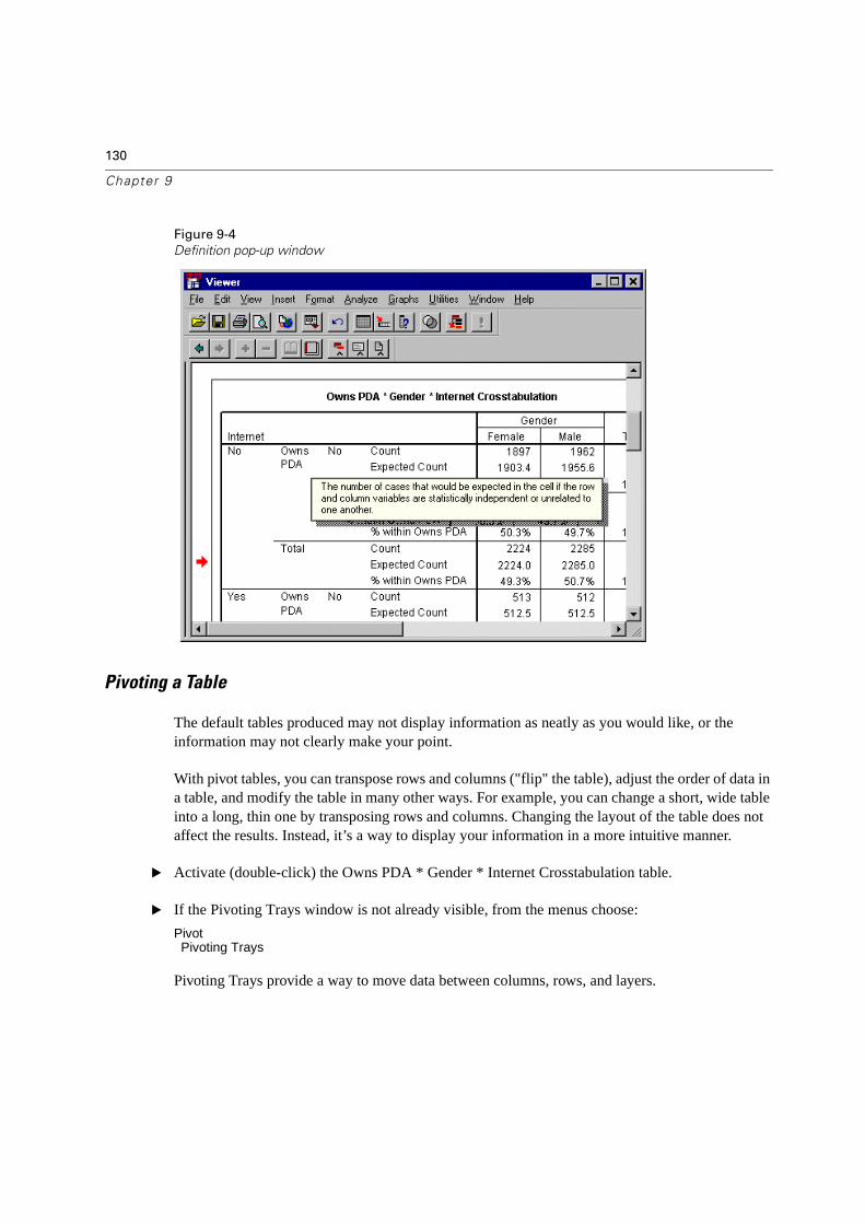
130
Chapter 9
Figure 9-4
Definition pop-up window
Pivoting a Table
The default tables produced may not display information as neatly as you would like, or the information may not clearly make your point.
With pivot tables, you can transpose rows and columns ("flip" the table), adjust the order of data in a table, and modify the table in many other ways. For example, you can change a short, wide table into a long, thin one by transposing rows and columns. Changing the layout of the table does not affect the results. Instead, it’s a way to display your information in a more intuitive manner.
� Activate (double-click) the Owns PDA * Gender * Internet Crosstabulation table.
� If the Pivoting Trays window is not already visible, from the menus choose:
PivotPivoting Trays
Pivoting Trays provide a way to move data between columns, rows, and layers.
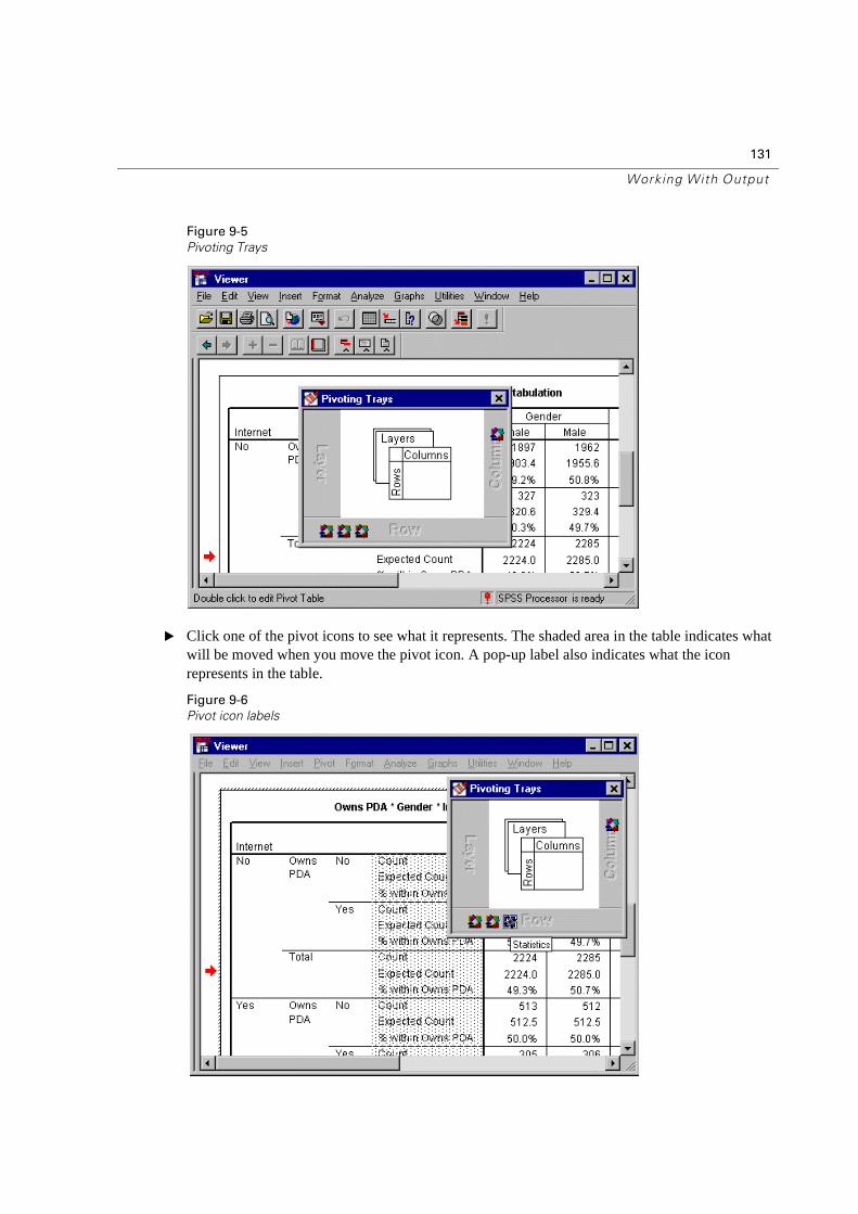
131
Working With Output
Figure 9-5
Pivoting Trays
� Click one of the pivot icons to see what it represents. The shaded area in the table indicates what will be moved when you move the pivot icon. A pop-up label also indicates what the icon represents in the table.
Figure 9-6
Pivot icon labels
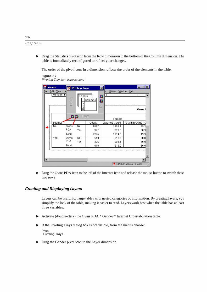
132
Chapter 9
� Drag the Statistics pivot icon from the Row dimension to the bottom of the Column dimension. The table is immediately reconfigured to reflect your changes.
The order of the pivot icons in a dimension reflects the order of the elements in the table.
Figure 9-7
Pivoting Tray icon associations
� Drag the Owns PDA icon to the left of the Internet icon and release the mouse button to switch these two rows
Creating and Displaying Layers
Layers can be useful for large tables with nested categories of information. By creating layers, you simplify the look of the table, making it easier to read. Layers work best when the table has at least three variables.
� Activate (double-click) the Owns PDA * Gender * Internet Crosstabulation table.
� If the Pivoting Trays dialog box is not visible, from the menus choose:
PivotPivoting Trays
� Drag the Gender pivot icon to the Layer dimension.
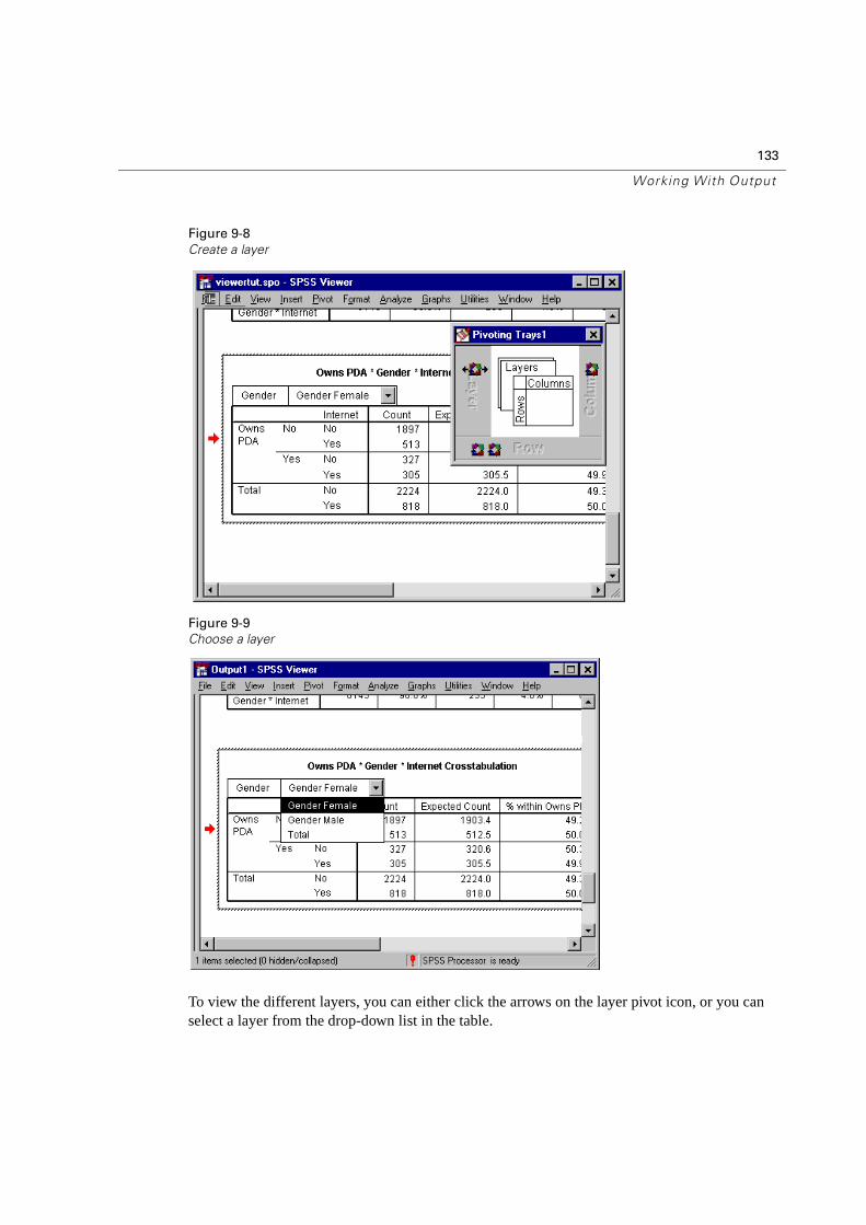
133
Working With Output
Figure 9-8
Create a layer
Figure 9-9
Choose a layer
To view the different layers, you can either click the arrows on the layer pivot icon, or you can select a layer from the drop-down list in the table.

134
Chapter 9
Editing Tables
Unless you’ve taken the time to create a custom TableLook, pivot tables are created with standard formatting. You can change the formatting of any text within a table. This includes changing the font size, color, and adding additional formatting, such as bolding or italics.
� Activate (double-click) the Level of education table.
� If the Formatting toolbar is not visible, from the menus choose:
ViewToolbar
� Click the title text, Level of education.
� Select 12 from the list of font sizes on the toolbar to increase the font size to 12 points.
� Select a new color for the label from the Text Color control.
Figure 9-10
Change the font color
You can also edit the contents of tables and labels. For example, you can change the title of this table.
� Activate (double-click) the title.
� Type Education Level for the new label.
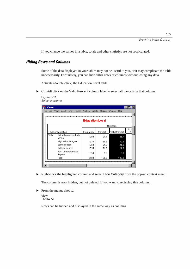
135
Working With Output
If you change the values in a table, totals and other statistics are not recalculated.
Hiding Rows and Columns
Some of the data displayed in your tables may not be useful to you, or it may complicate the table unnecessarily. Fortunately, you can hide entire rows or columns without losing any data.
Activate (double-click) the Education Level table.
� Ctrl-Alt click on the Valid Percent column label to select all the cells in that column.
Figure 9-11
Select a column
� Right-click the highlighted column and select Hide Category from the pop-up context menu.
The column is now hidden, but not deleted. If you want to redisplay this column...
� From the menus choose:
ViewShow All
Rows can be hidden and displayed in the same way as columns.
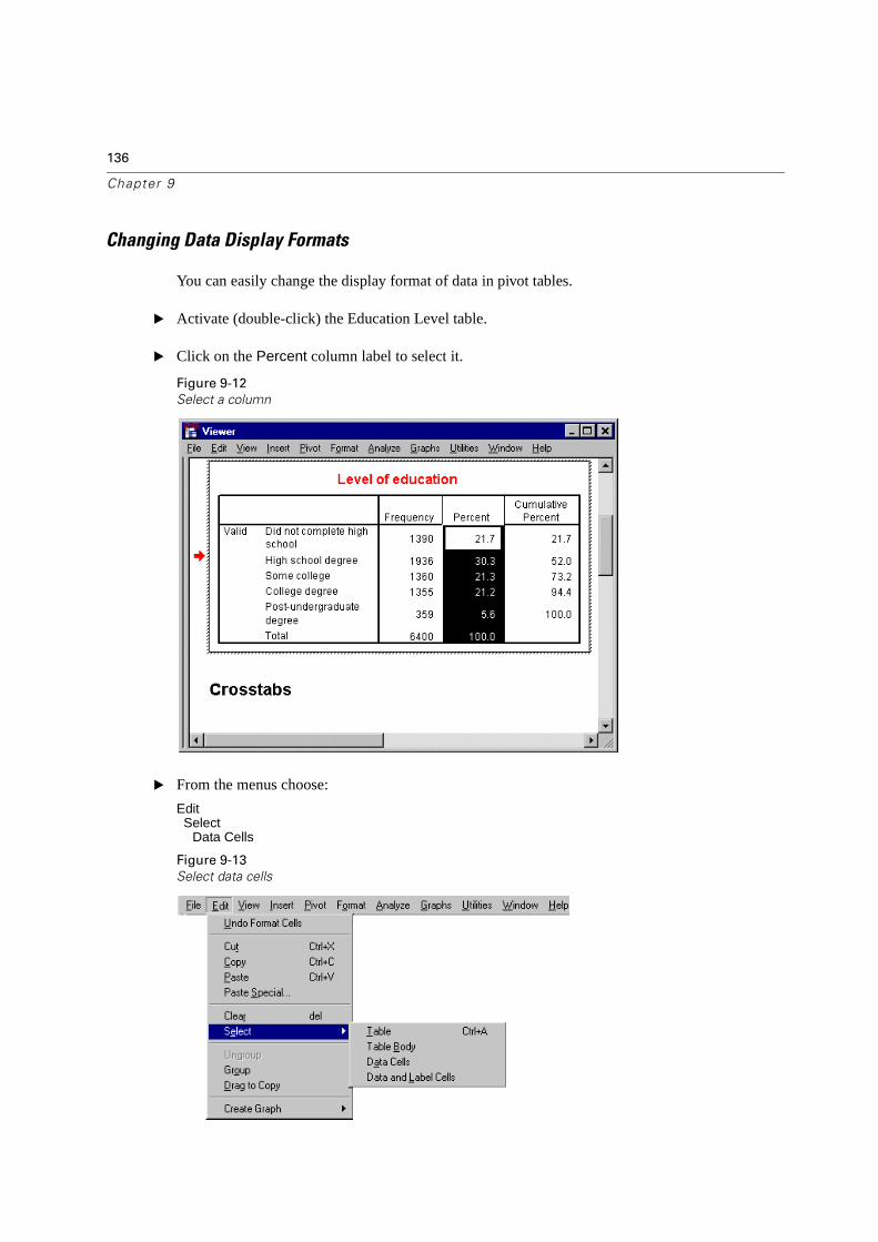
136
Chapter 9
Changing Data Display Formats
You can easily change the display format of data in pivot tables.
� Activate (double-click) the Education Level table.
� Click on the Percent column label to select it.
Figure 9-12
Select a column
� From the menus choose:
EditSelect
Data Cells
Figure 9-13
Select data cells
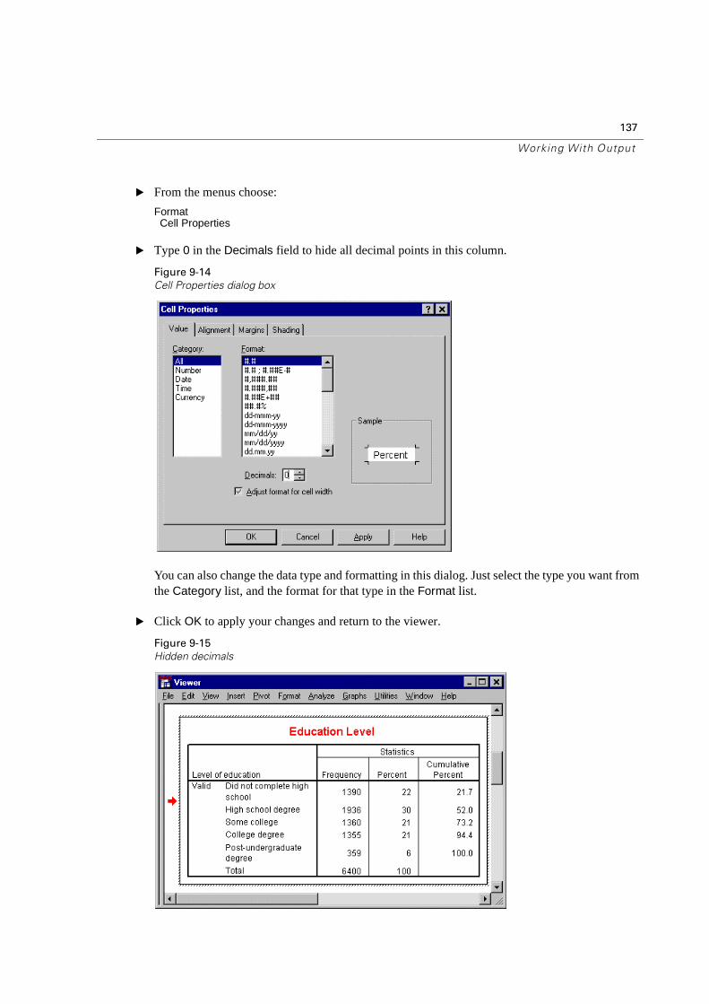
137
Working With Output
� From the menus choose:
FormatCell Properties
� Type 0 in the Decimals field to hide all decimal points in this column.
Figure 9-14
Cell Properties dialog box
You can also change the data type and formatting in this dialog. Just select the type you want from the Category list, and the format for that type in the Format list.
� Click OK to apply your changes and return to the viewer.
Figure 9-15
Hidden decimals
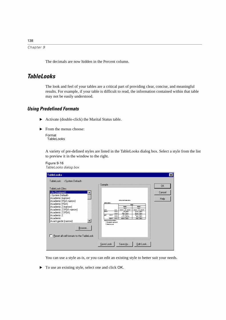
138
Chapter 9
The decimals are now hidden in the Percent column.
TableLooks
The look and feel of your tables are a critical part of providing clear, concise, and meaningful results. For example, if your table is difficult to read, the information contained within that table may not be easily understood.
Using Predefined Formats
� Activate (double-click) the Marital Status table.
� From the menus choose:
FormatTableLooks
A variety of pre-defined styles are listed in the TableLooks dialog box. Select a style from the list to preview it in the window to the right.
Figure 9-16
TableLooks dialog box
You can use a style as-is, or you can edit an existing style to better suit your needs.
� To use an existing style, select one and click OK.
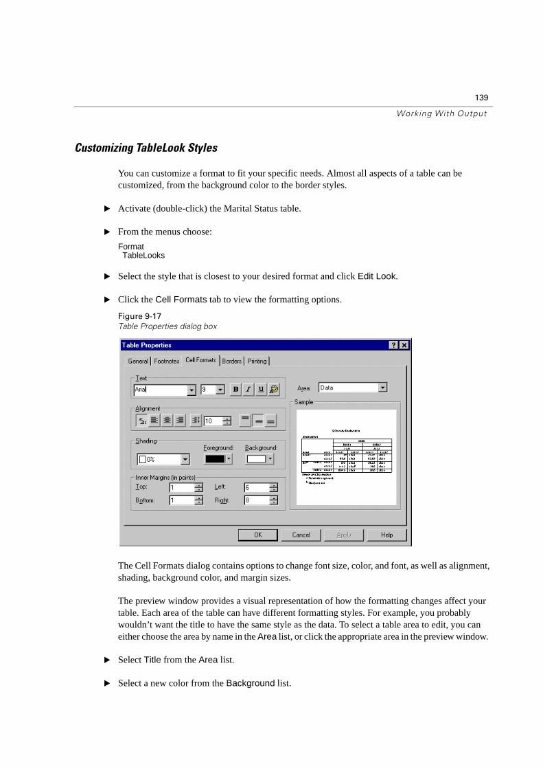
139
Working With Output
Customizing TableLook Styles
You can customize a format to fit your specific needs. Almost all aspects of a table can be customized, from the background color to the border styles.
� Activate (double-click) the Marital Status table.
� From the menus choose:
FormatTableLooks
� Select the style that is closest to your desired format and click Edit Look.
� Click the Cell Formats tab to view the formatting options.
Figure 9-17
Table Properties dialog box
The Cell Formats dialog contains options to change font size, color, and font, as well as alignment, shading, background color, and margin sizes.
The preview window provides a visual representation of how the formatting changes affect your table. Each area of the table can have different formatting styles. For example, you probably wouldn’t want the title to have the same style as the data. To select a table area to edit, you can either choose the area by name in the Area list, or click the appropriate area in the preview window.
� Select Title from the Area list.
� Select a new color from the Background list.
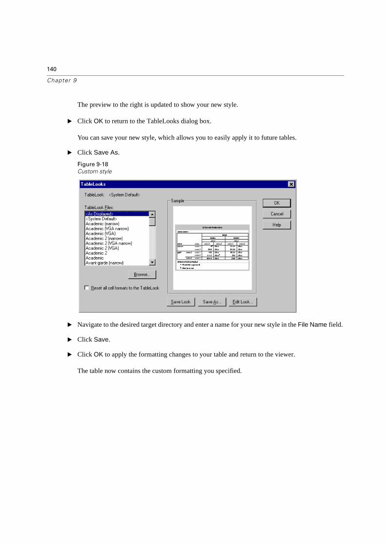
140
Chapter 9
The preview to the right is updated to show your new style.
� Click OK to return to the TableLooks dialog box.
You can save your new style, which allows you to easily apply it to future tables.
� Click Save As.
Figure 9-18
Custom style
� Navigate to the desired target directory and enter a name for your new style in the File Name field.
� Click Save.
� Click OK to apply the formatting changes to your table and return to the viewer.
The table now contains the custom formatting you specified.
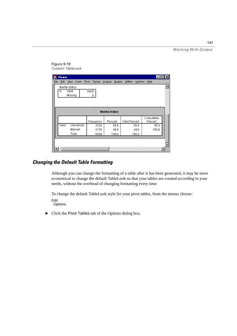
141
Working With Output
Figure 9-19
Custom TableLook
Changing the Default Table Formatting
Although you can change the formatting of a table after it has been generated, it may be more economical to change the default TableLook so that your tables are created according to your needs, without the overhead of changing formatting every time.
To change the default TableLook style for your pivot tables, from the menus choose:
EditOptions
� Click the Pivot Tables tab of the Options dialog box.
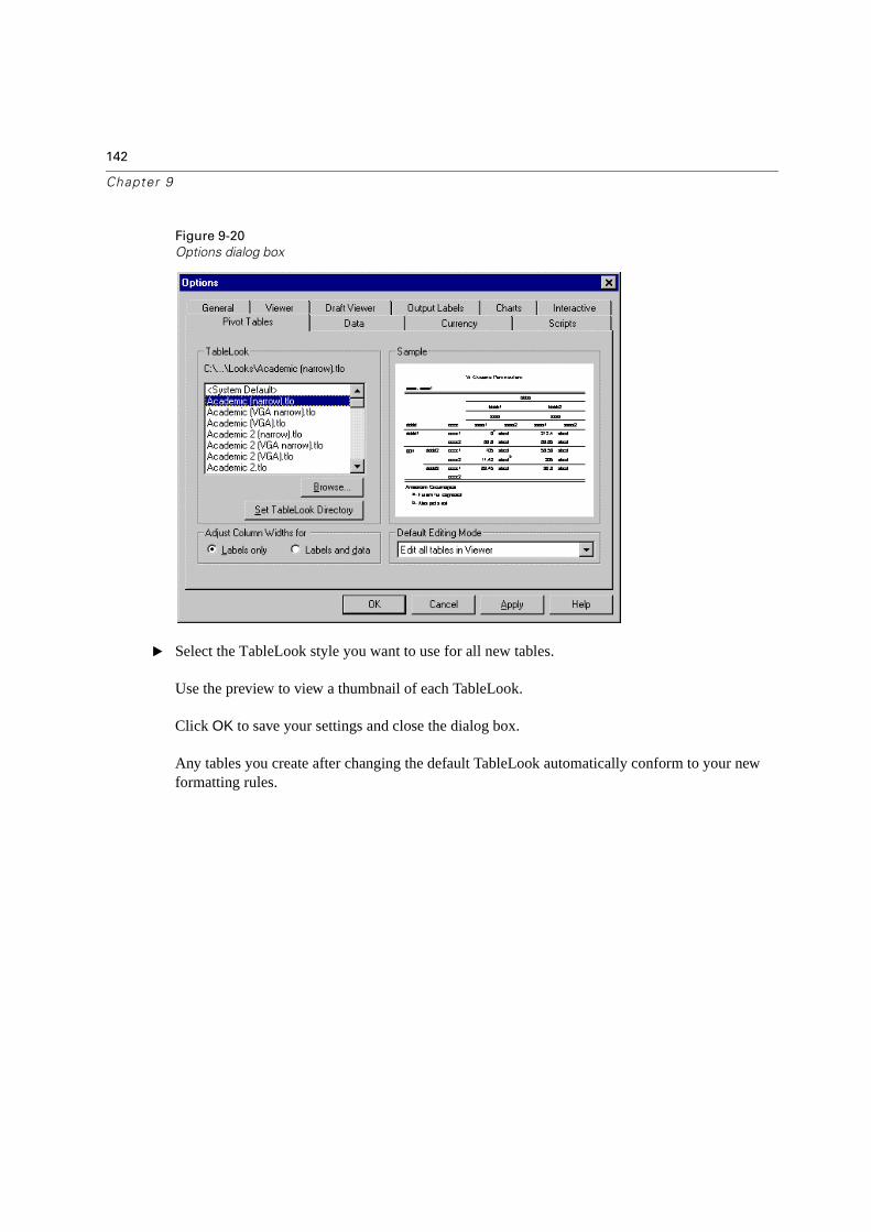
142
Chapter 9
Figure 9-20
Options dialog box
� Select the TableLook style you want to use for all new tables.
Use the preview to view a thumbnail of each TableLook.
Click OK to save your settings and close the dialog box.
Any tables you create after changing the default TableLook automatically conform to your new formatting rules.
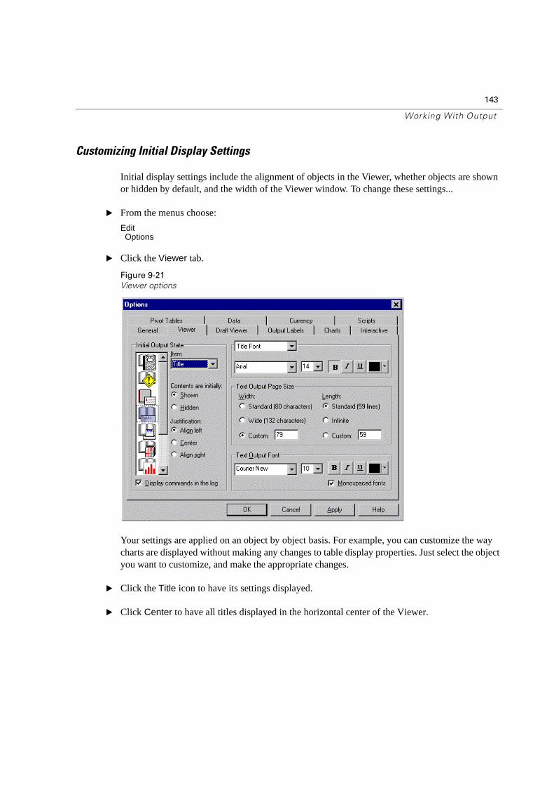
143
Working With Output
Customizing Initial Display Settings
Initial display settings include the alignment of objects in the Viewer, whether objects are shown or hidden by default, and the width of the Viewer window. To change these settings...
� From the menus choose:
EditOptions
� Click the Viewer tab.
Figure 9-21
Viewer options
Your settings are applied on an object by object basis. For example, you can customize the way charts are displayed without making any changes to table display properties. Just select the object you want to customize, and make the appropriate changes.
� Click the Title icon to have its settings displayed.
� Click Center to have all titles displayed in the horizontal center of the Viewer.
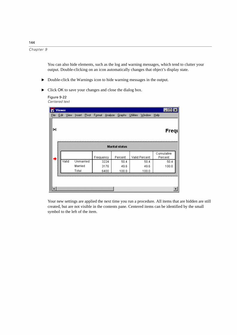
144
Chapter 9
You can also hide elements, such as the log and warning messages, which tend to clutter your output. Double-clicking on an icon automatically changes that object’s display state.
� Double-click the Warnings icon to hide warning messages in the output.
� Click OK to save your changes and close the dialog box.
Figure 9-22
Centered text
Your new settings are applied the next time you run a procedure. All items that are hidden are still created, but are not visible in the contents pane. Centered items can be identified by the small symbol to the left of the item.
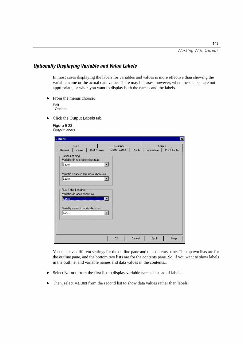
145
Working With Output
Optionally Displaying Variable and Value Labels
In most cases displaying the labels for variables and values is more effective than showing the variable name or the actual data value. There may be cases, however, when these labels are not appropriate, or when you want to display both the names and the labels.
� From the menus choose:
EditOptions
� Click the Output Labels tab.
Figure 9-23
Output labels
You can have different settings for the outline pane and the contents pane. The top two lists are for the outline pane, and the bottom two lists are for the contents pane. So, if you want to show labels in the outline, and variable names and data values in the contents...
� Select Names from the first list to display variable names instead of labels.
� Then, select Values from the second list to show data values rather than labels.
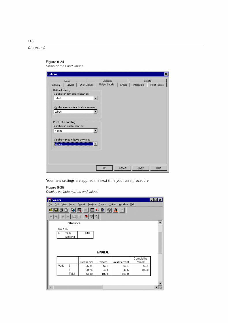
146
Chapter 9
Figure 9-24
Show names and values
Your new settings are applied the next time you run a procedure.
Figure 9-25
Display variable names and values
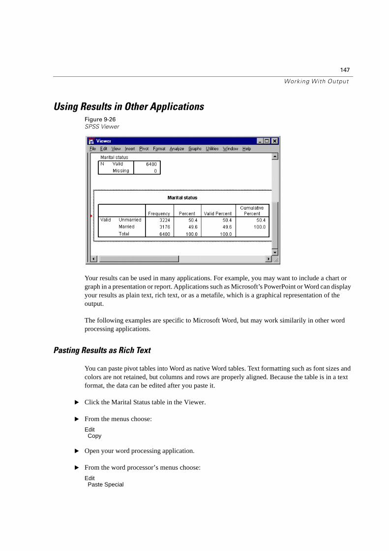
147
Working With Output
Using Results in Other ApplicationsFigure 9-26
SPSS Viewer
Your results can be used in many applications. For example, you may want to include a chart or graph in a presentation or report. Applications such as Microsoft’s PowerPoint or Word can display your results as plain text, rich text, or as a metafile, which is a graphical representation of the output.
The following examples are specific to Microsoft Word, but may work similarily in other word processing applications.
Pasting Results as Rich Text
You can paste pivot tables into Word as native Word tables. Text formatting such as font sizes and colors are not retained, but columns and rows are properly aligned. Because the table is in a text format, the data can be edited after you paste it.
� Click the Marital Status table in the Viewer.
� From the menus choose:
EditCopy
� Open your word processing application.
� From the word processor’s menus choose:
EditPaste Special
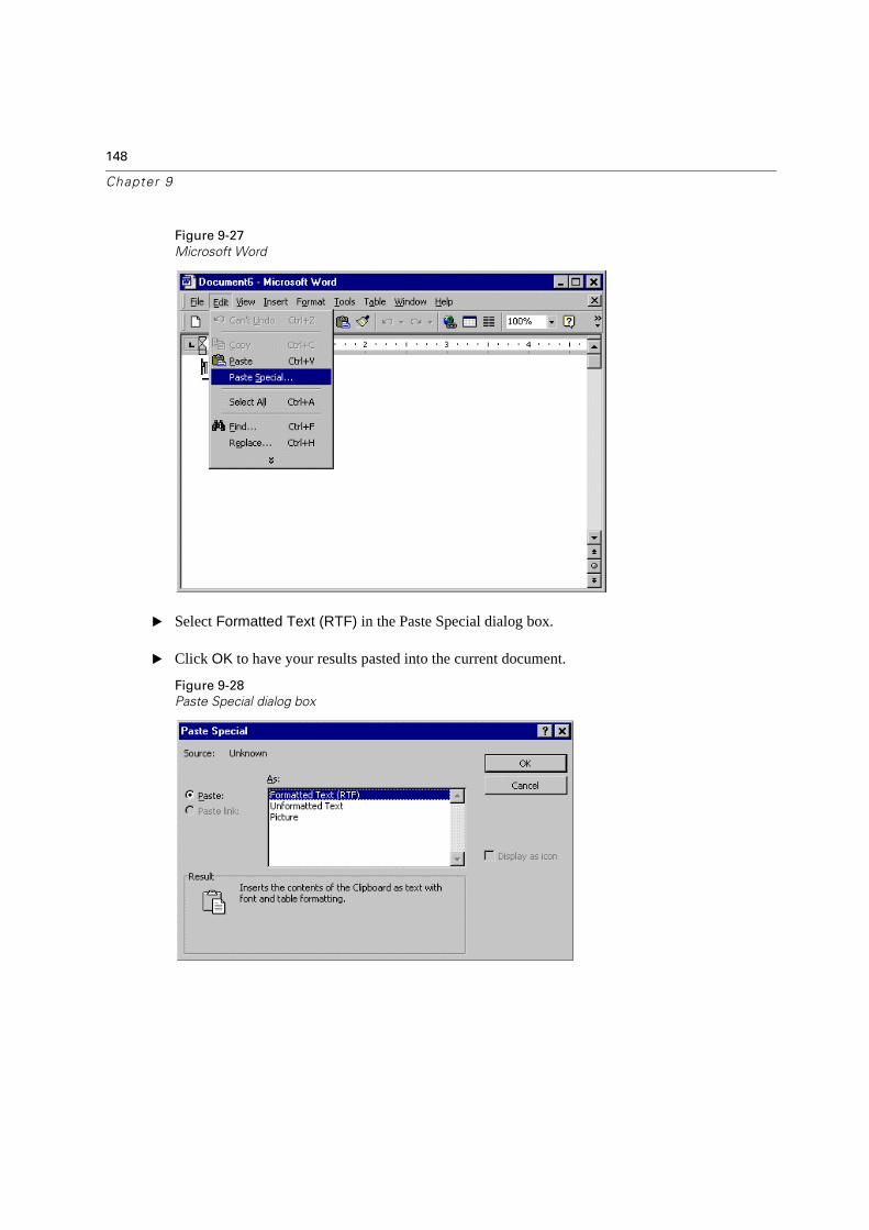
148
Chapter 9
Figure 9-27
Microsoft Word
� Select Formatted Text (RTF) in the Paste Special dialog box.
� Click OK to have your results pasted into the current document.
Figure 9-28
Paste Special dialog box
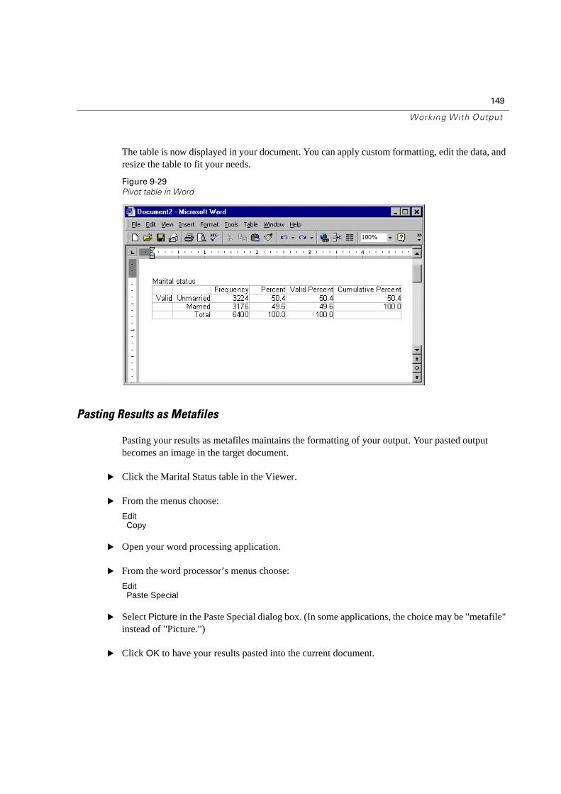
149
Working With Output
The table is now displayed in your document. You can apply custom formatting, edit the data, and resize the table to fit your needs.
Figure 9-29
Pivot table in Word
Pasting Results as Metafiles
Pasting your results as metafiles maintains the formatting of your output. Your pasted output becomes an image in the target document.
� Click the Marital Status table in the Viewer.
� From the menus choose:
EditCopy
� Open your word processing application.
� From the word processor’s menus choose:
EditPaste Special
� Select Picture in the Paste Special dialog box. (In some applications, the choice may be "metafile" instead of "Picture.")
� Click OK to have your results pasted into the current document.
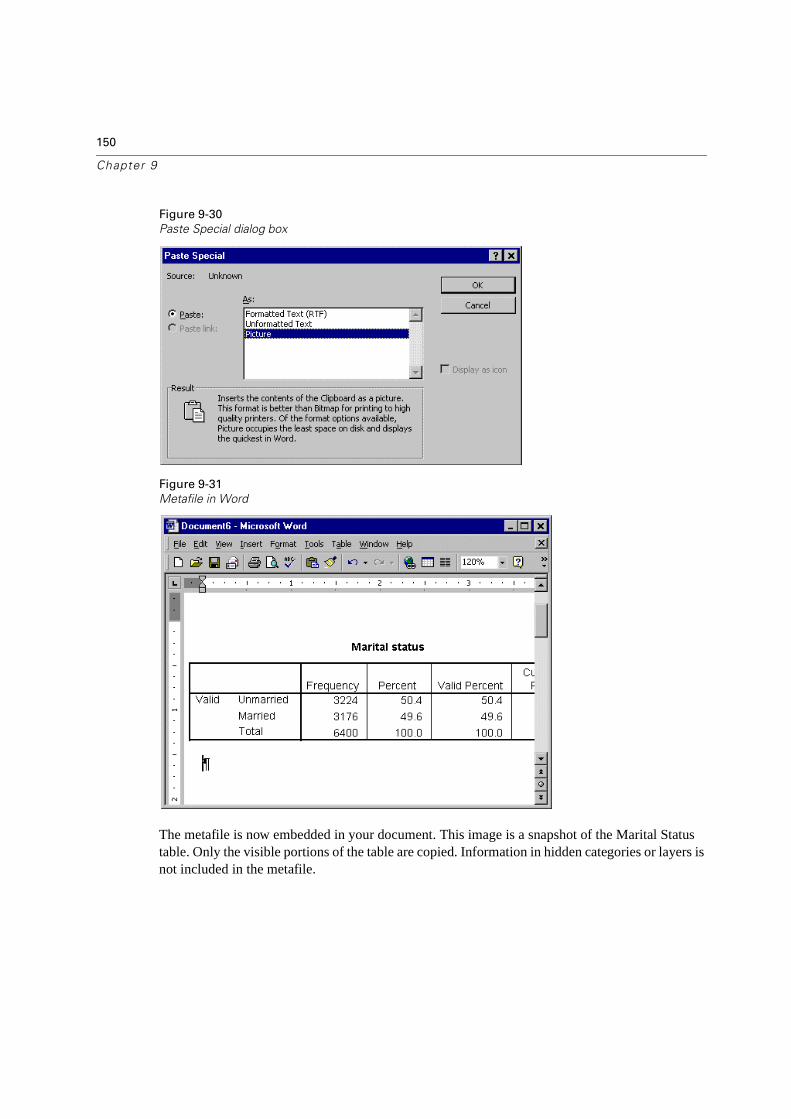
150
Chapter 9
Figure 9-30
Paste Special dialog box
Figure 9-31
Metafile in Word
The metafile is now embedded in your document. This image is a snapshot of the Marital Status table. Only the visible portions of the table are copied. Information in hidden categories or layers is not included in the metafile.
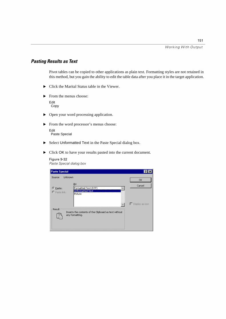
151
Working With Output
Pasting Results as Text
Pivot tables can be copied to other applications as plain text. Formatting styles are not retained in this method, but you gain the ability to edit the table data after you place it in the target application.
� Click the Marital Status table in the Viewer.
� From the menus choose:
EditCopy
� Open your word processing application.
� From the word processor’s menus choose:
EditPaste Special
� Select Unformatted Text in the Paste Special dialog box.
� Click OK to have your results pasted into the current document.
Figure 9-32
Paste Special dialog box
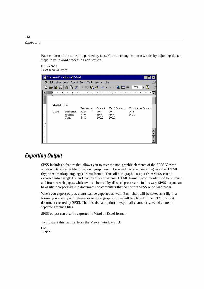
152
Chapter 9
Each column of the table is separated by tabs. You can change column widths by adjusting the tab stops in your word processing application.
Figure 9-33
Pivot table in Word
Exporting Output
SPSS includes a feature that allows you to save the non-graphic elements of the SPSS Viewer window into a single file (note: each graph would be saved into a separate file) in either HTML (hypertext markup language) or text format. Thus all non-graphic output from SPSS can be exported into a single file and read by other programs. HTML format is commonly used for intranet and Internet web pages, while text can be read by all word processors. In this way, SPSS output can be easily incorporated into documents on computers that do not run SPSS or on web pages.
When you export output, charts can be exported as well. Each chart will be saved as a file in a format you specify and references to these graphics files will be placed in the HTML or text document created by SPSS. There is also an option to export all charts, or selected charts, in separate graphics files.
SPSS output can also be exported in Word or Excel format.
To illustrate this feature, from the Viewer window click:
FileExport
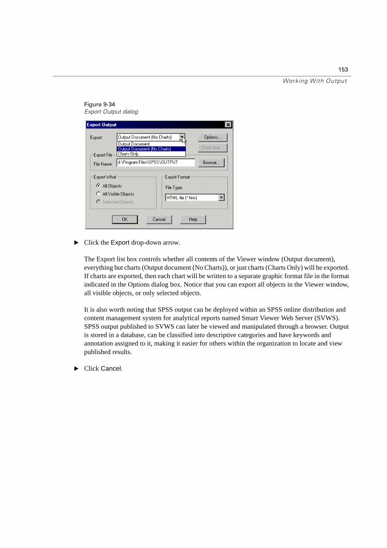
153
Working With Output
Figure 9-34
Export Output dialog
� Click the Export drop-down arrow.
The Export list box controls whether all contents of the Viewer window (Output document), everything but charts (Output document (No Charts)), or just charts (Charts Only) will be exported. If charts are exported, then each chart will be written to a separate graphic format file in the format indicated in the Options dialog box. Notice that you can export all objects in the Viewer window, all visible objects, or only selected objects.
It is also worth noting that SPSS output can be deployed within an SPSS online distribution and content management system for analytical reports named Smart Viewer Web Server (SVWS). SPSS output published to SVWS can later be viewed and manipulated through a browser. Output is stored in a database, can be classified into descriptive categories and have keywords and annotation assigned to it, making it easier for others within the organization to locate and view published results.
� Click Cancel.

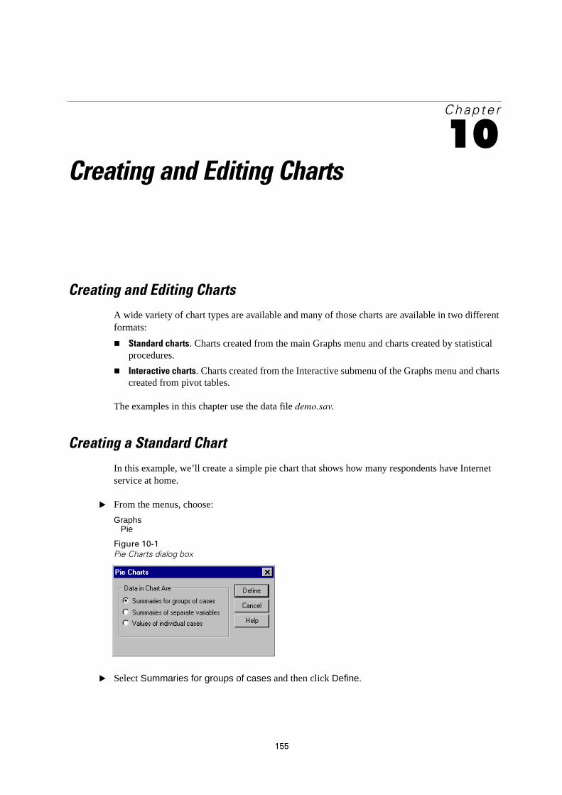
155
Chapte r
10Creating and Editing Charts
Creating and Editing Charts
A wide variety of chart types are available and many of those charts are available in two different formats:
� Standard charts. Charts created from the main Graphs menu and charts created by statistical procedures.
� Interactive charts. Charts created from the Interactive submenu of the Graphs menu and charts created from pivot tables.
The examples in this chapter use the data file demo.sav.
Creating a Standard Chart
In this example, we’ll create a simple pie chart that shows how many respondents have Internet service at home.
� From the menus, choose:
Graphs Pie
Figure 10-1
Pie Charts dialog box
� Select Summaries for groups of cases and then click Define.
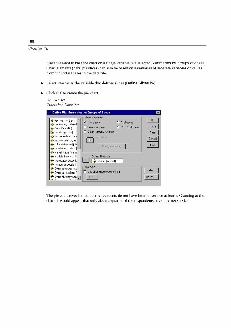
156
Chapter 10
Since we want to base the chart on a single variable, we selected Summaries for groups of cases.Chart elements (bars, pie slices) can also be based on summaries of separate variables or values from individual cases in the data file.
� Select Internet as the variable that defines slices (Define Slices by).
� Click OK to create the pie chart.
Figure 10-2
Define Pie dialog box
The pie chart reveals that most respondents do not have Internet service at home. Glancing at the chart, it would appear that only about a quarter of the respondents have Internet service.
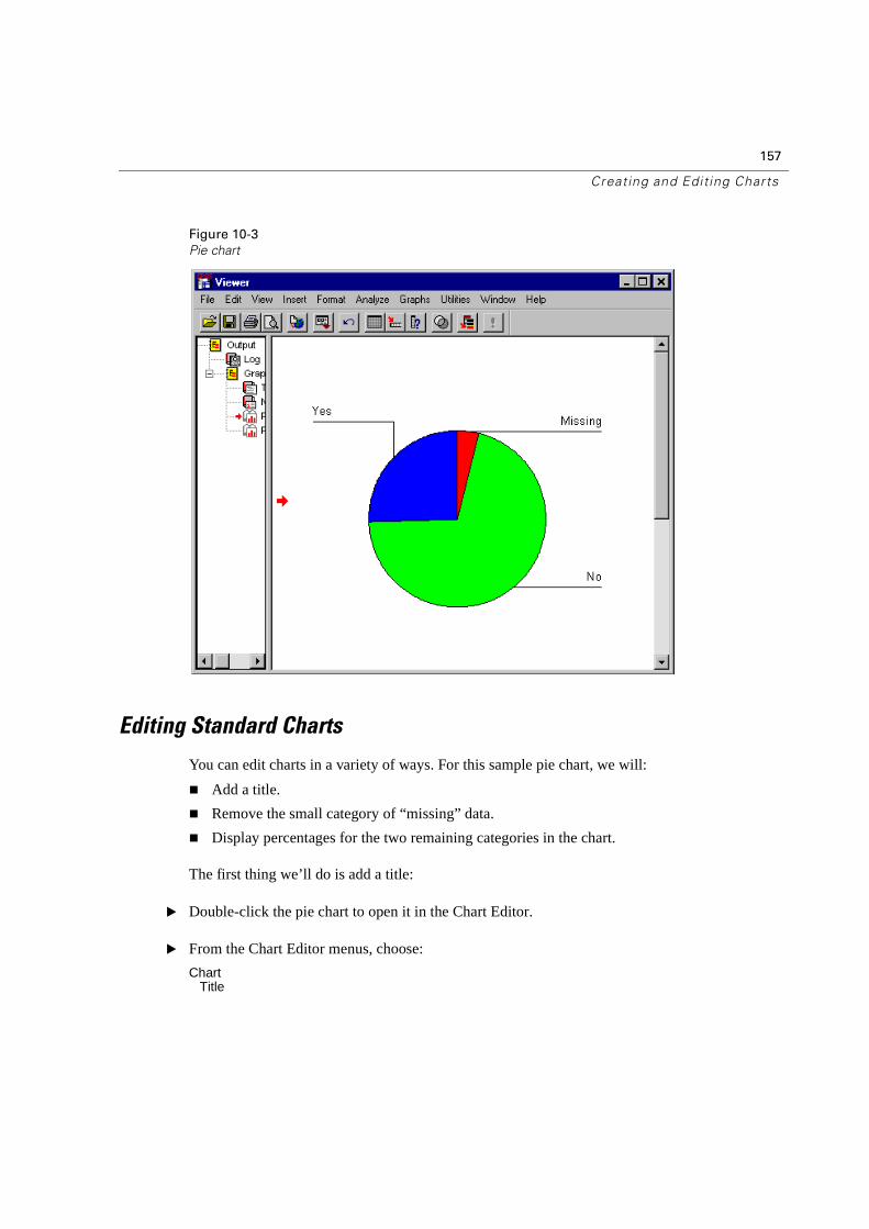
157
Creating and Editing Charts
Figure 10-3
Pie chart
Editing Standard Charts
You can edit charts in a variety of ways. For this sample pie chart, we will:
� Add a title.
� Remove the small category of “missing” data.
� Display percentages for the two remaining categories in the chart.
The first thing we’ll do is add a title:
� Double-click the pie chart to open it in the Chart Editor.
� From the Chart Editor menus, choose:
Chart Title
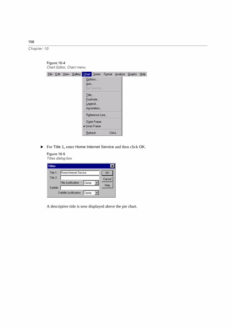
158
Chapter 10
Figure 10-4
Chart Editor, Chart menu
� For Title 1, enter Home Internet Service and then click OK.
Figure 10-5
Titles dialog box
A descriptive title is now displayed above the pie chart.
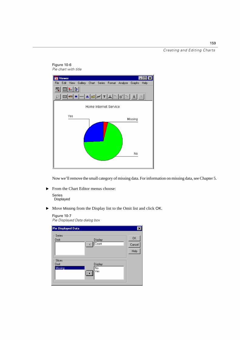
159
Creating and Editing Charts
Figure 10-6
Pie chart with title
Now we’ll remove the small category of missing data. For information on missing data, see Chapter 5.
� From the Chart Editor menus choose:
SeriesDisplayed
� Move Missing from the Display list to the Omit list and click OK.
Figure 10-7
Pie Displayed Data dialog box
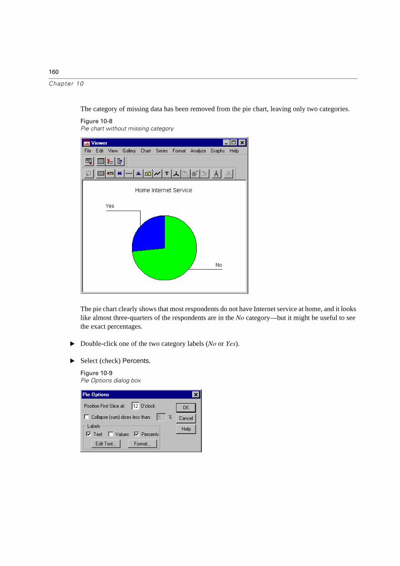
160
Chapter 10
The category of missing data has been removed from the pie chart, leaving only two categories.
Figure 10-8
Pie chart without missing category
The pie chart clearly shows that most respondents do not have Internet service at home, and it looks like almost three-quarters of the respondents are in the No category—but it might be useful to see the exact percentages.
� Double-click one of the two category labels (No or Yes).
� Select (check) Percents.
Figure 10-9
Pie Options dialog box
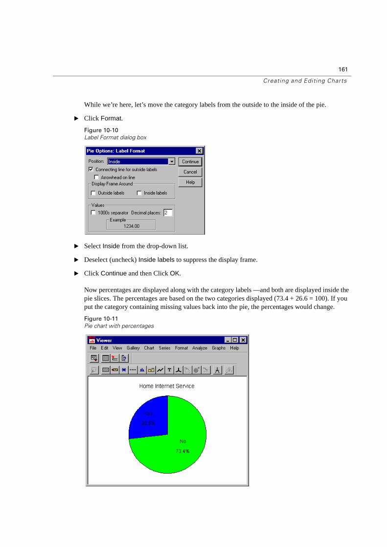
161
Creating and Editing Charts
While we’re here, let’s move the category labels from the outside to the inside of the pie.
� Click Format.
Figure 10-10
Label Format dialog box
� Select Inside from the drop-down list.
� Deselect (uncheck) Inside labels to suppress the display frame.
� Click Continue and then Click OK.
Now percentages are displayed along with the category labels —and both are displayed inside the pie slices. The percentages are based on the two categories displayed (73.4 + 26.6 = 100). If you put the category containing missing values back into the pie, the percentages would change.
Figure 10-11
Pie chart with percentages
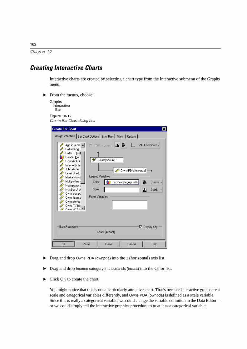
162
Chapter 10
Creating Interactive Charts
Interactive charts are created by selecting a chart type from the Interactive submenu of the Graphs menu.
� From the menus, choose:
Graphs Interactive
Bar
Figure 10-12
Create Bar Chart dialog box
� Drag and drop Owns PDA (ownpda) into the x (horizontal) axis list.
� Drag and drop Income category in thousands (inccat) into the Color list.
� Click OK to create the chart.
You might notice that this is not a particularly attractive chart. That’s because interactive graphs treat scale and categorical variables differently, and Owns PDA (ownpda) is defined as a scale variable. Since this is really a categorical variable, we could change the variable definition in the Data Editor—or we could simply tell the interactive graphics procedure to treat it as a categorical variable.
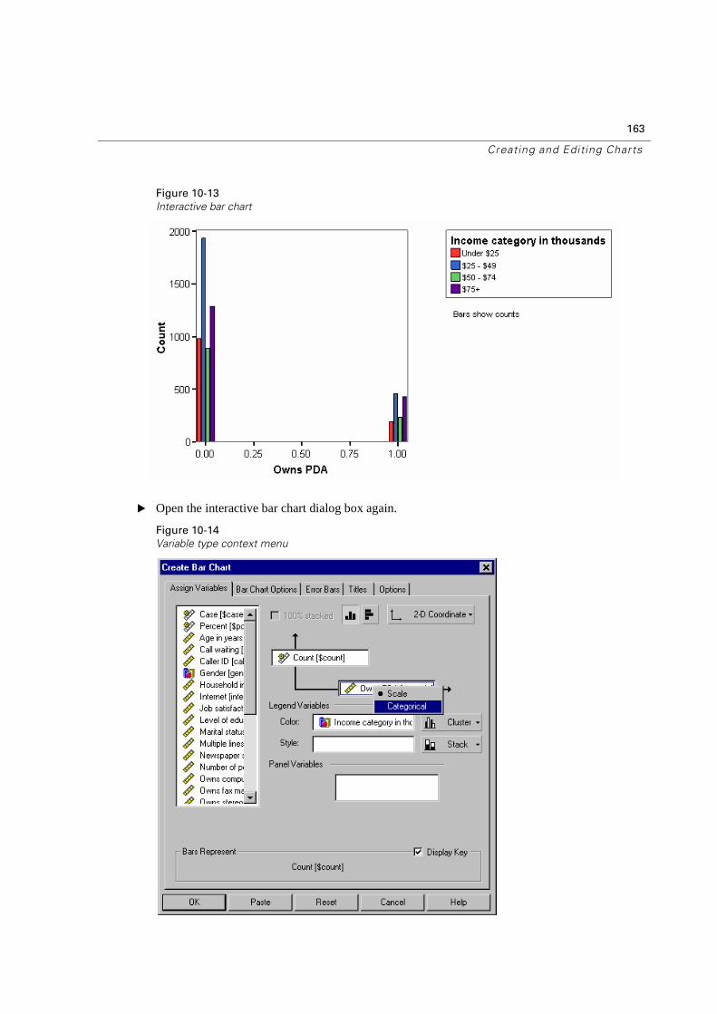
163
Creating and Editing Charts
Figure 10-13
Interactive bar chart
� Open the interactive bar chart dialog box again.
Figure 10-14
Variable type context menu
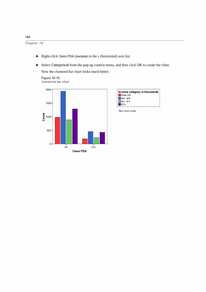
164
Chapter 10
� Right-click Owns PDA (ownpda) in the x (horizontal) axis list.
� Select Categorical from the pop-up context menu, and then click OK to create the chart.
Now the clustered bar chart looks much better.
Figure 10-15
Interactive bar chart
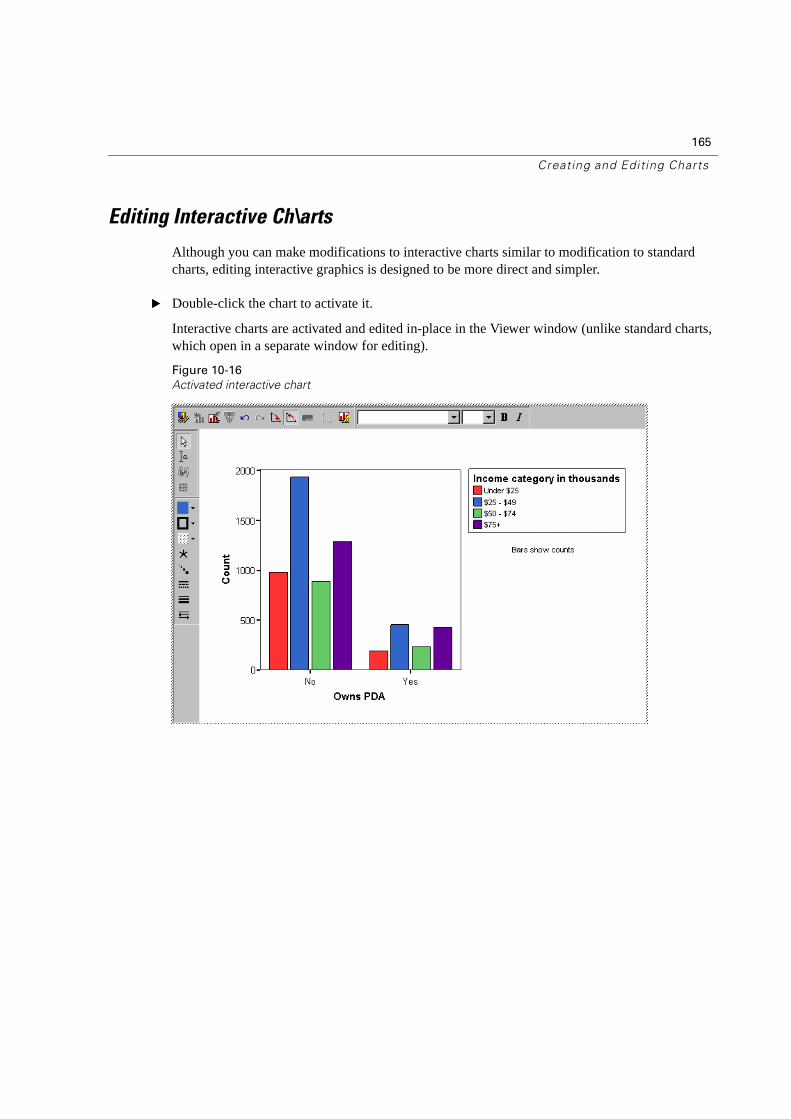
165
Creating and Editing Charts
Editing Interactive Ch\arts
Although you can make modifications to interactive charts similar to modification to standard charts, editing interactive graphics is designed to be more direct and simpler.
� Double-click the chart to activate it.
Interactive charts are activated and edited in-place in the Viewer window (unlike standard charts, which open in a separate window for editing).
Figure 10-16
Activated interactive chart
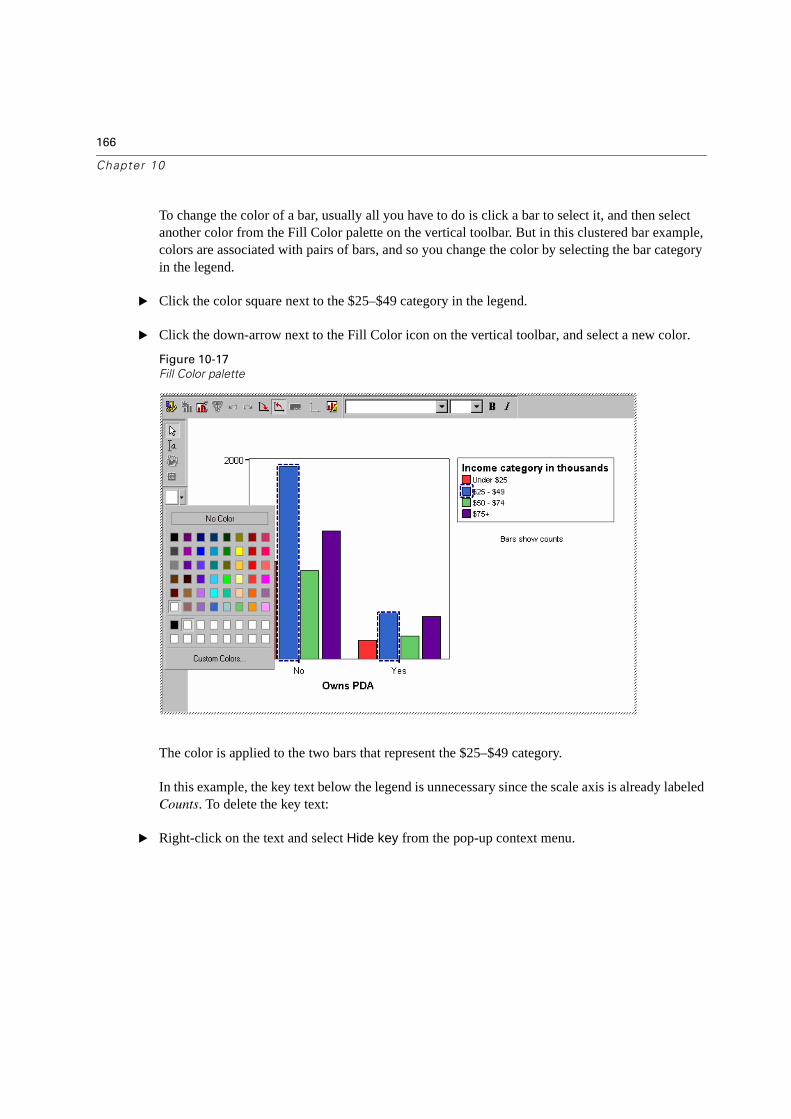
166
Chapter 10
To change the color of a bar, usually all you have to do is click a bar to select it, and then select another color from the Fill Color palette on the vertical toolbar. But in this clustered bar example, colors are associated with pairs of bars, and so you change the color by selecting the bar category in the legend.
� Click the color square next to the $25–$49 category in the legend.
� Click the down-arrow next to the Fill Color icon on the vertical toolbar, and select a new color.
Figure 10-17
Fill Color palette
The color is applied to the two bars that represent the $25–$49 category.
In this example, the key text below the legend is unnecessary since the scale axis is already labeled Counts. To delete the key text:
� Right-click on the text and select Hide key from the pop-up context menu.
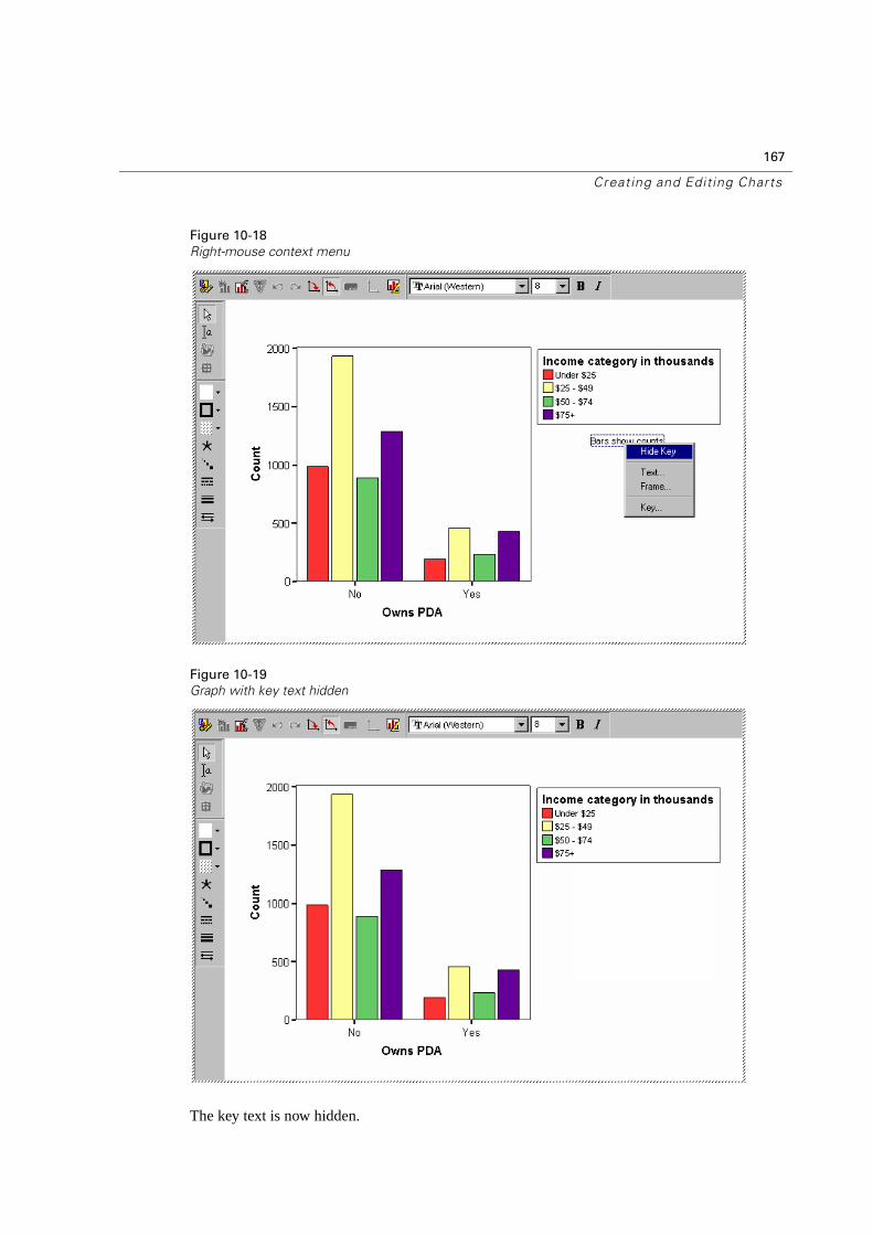
167
Creating and Editing Charts
Figure 10-18
Right-mouse context menu
Figure 10-19
Graph with key text hidden
The key text is now hidden.
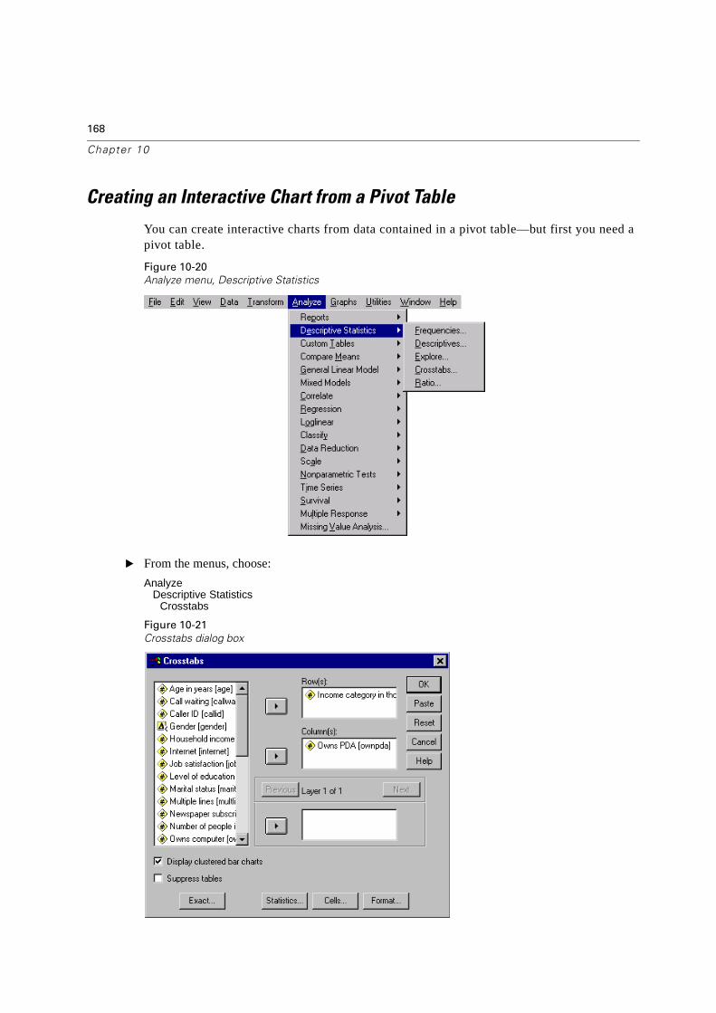
168
Chapter 10
Creating an Interactive Chart from a Pivot Table
You can create interactive charts from data contained in a pivot table—but first you need a pivot table.
Figure 10-20
Analyze menu, Descriptive Statistics
� From the menus, choose:
Analyze Descriptive Statistics
Crosstabs
Figure 10-21
Crosstabs dialog box
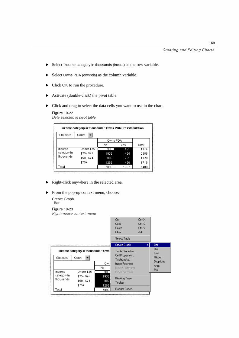
169
Creating and Editing Charts
� Select Income category in thousands (inccat) as the row variable.
� Select Owns PDA (ownpda) as the column variable.
� Click OK to run the procedure.
� Activate (double-click) the pivot table.
� Click and drag to select the data cells you want to use in the chart.
Figure 10-22
Data selected in pivot table
� Right-click anywhere in the selected area.
� From the pop-up context menu, choose:
Create GraphBar
Figure 10-23
Right-mouse context menu
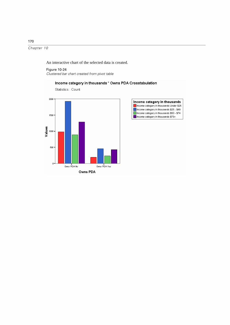
170
Chapter 10
An interactive chart of the selected data is created.
Figure 10-24
Clustered bar chart created from pivot table
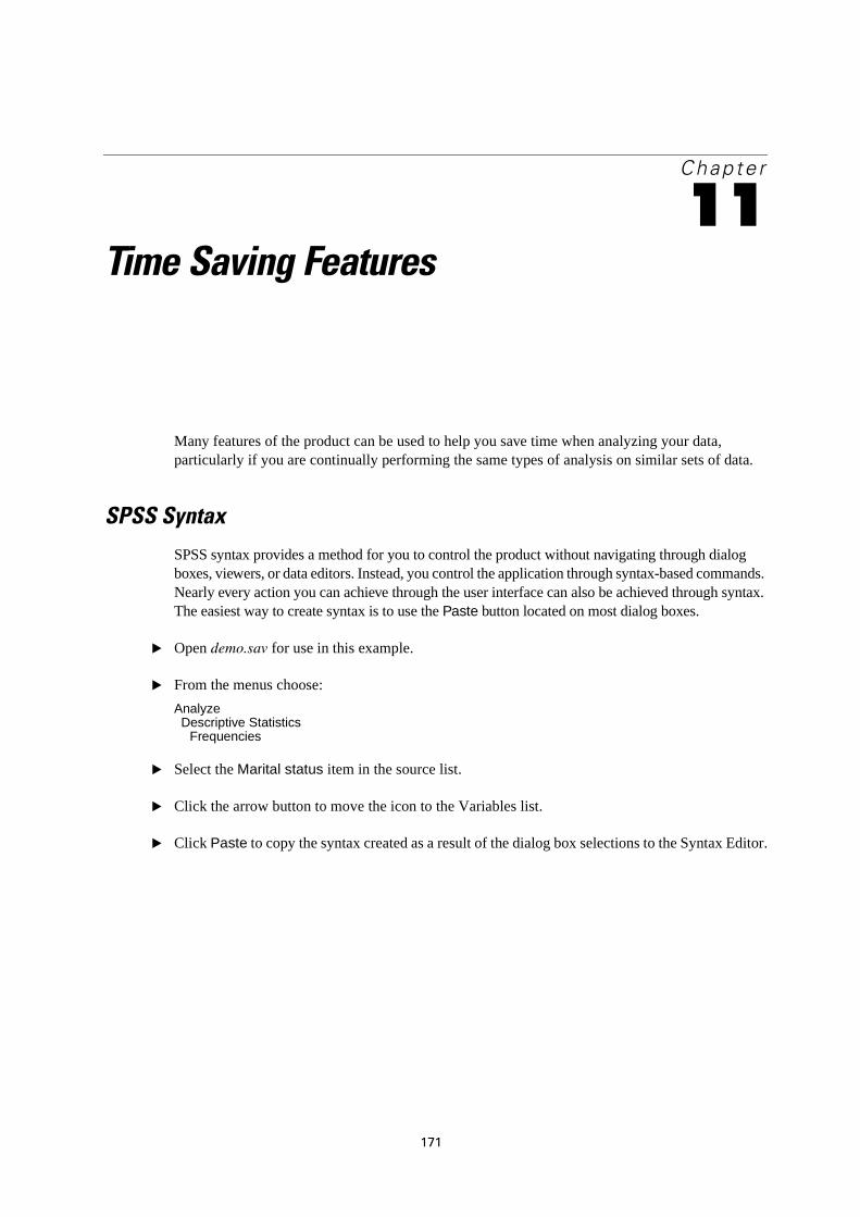
171
Chapte r
11Time Saving Features
Many features of the product can be used to help you save time when analyzing your data, particularly if you are continually performing the same types of analysis on similar sets of data.
SPSS Syntax
SPSS syntax provides a method for you to control the product without navigating through dialog boxes, viewers, or data editors. Instead, you control the application through syntax-based commands. Nearly every action you can achieve through the user interface can also be achieved through syntax. The easiest way to create syntax is to use the Paste button located on most dialog boxes.
� Open demo.sav for use in this example.
� From the menus choose:
AnalyzeDescriptive Statistics
Frequencies
� Select the Marital status item in the source list.
� Click the arrow button to move the icon to the Variables list.
� Click Paste to copy the syntax created as a result of the dialog box selections to the Syntax Editor.
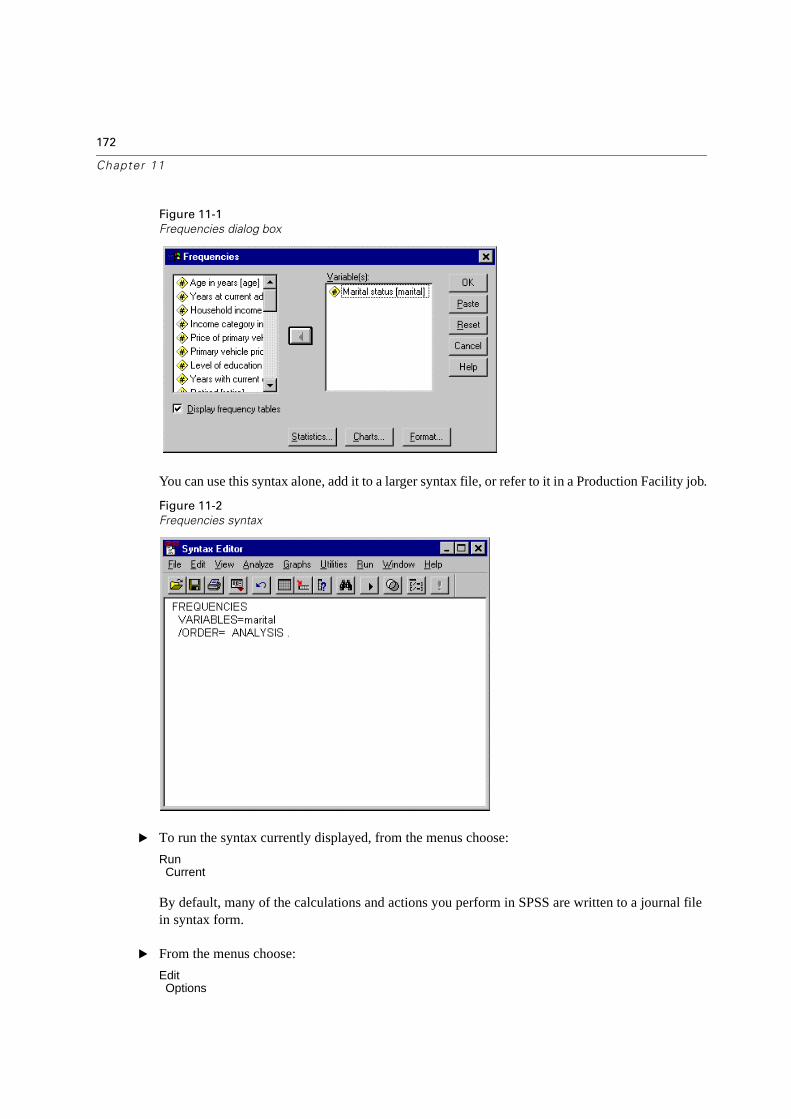
172
Chapter 11
Figure 11-1
Frequencies dialog box
You can use this syntax alone, add it to a larger syntax file, or refer to it in a Production Facility job.
Figure 11-2
Frequencies syntax
� To run the syntax currently displayed, from the menus choose:
RunCurrent
By default, many of the calculations and actions you perform in SPSS are written to a journal file in syntax form.
� From the menus choose:
EditOptions
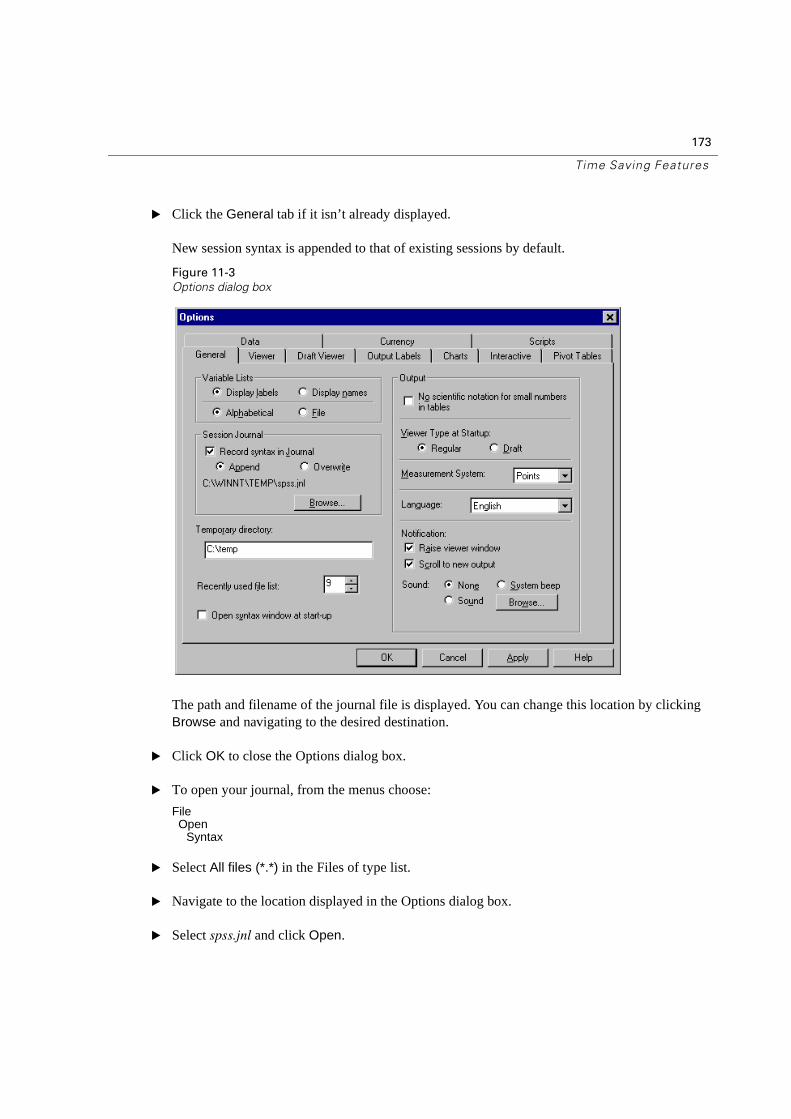
173
Time Saving Features
� Click the General tab if it isn’t already displayed.
New session syntax is appended to that of existing sessions by default.
Figure 11-3
Options dialog box
The path and filename of the journal file is displayed. You can change this location by clicking Browse and navigating to the desired destination.
� Click OK to close the Options dialog box.
� To open your journal, from the menus choose:
FileOpen
Syntax
� Select All files (*.*) in the Files of type list.
� Navigate to the location displayed in the Options dialog box.
� Select spss.jnl and click Open.
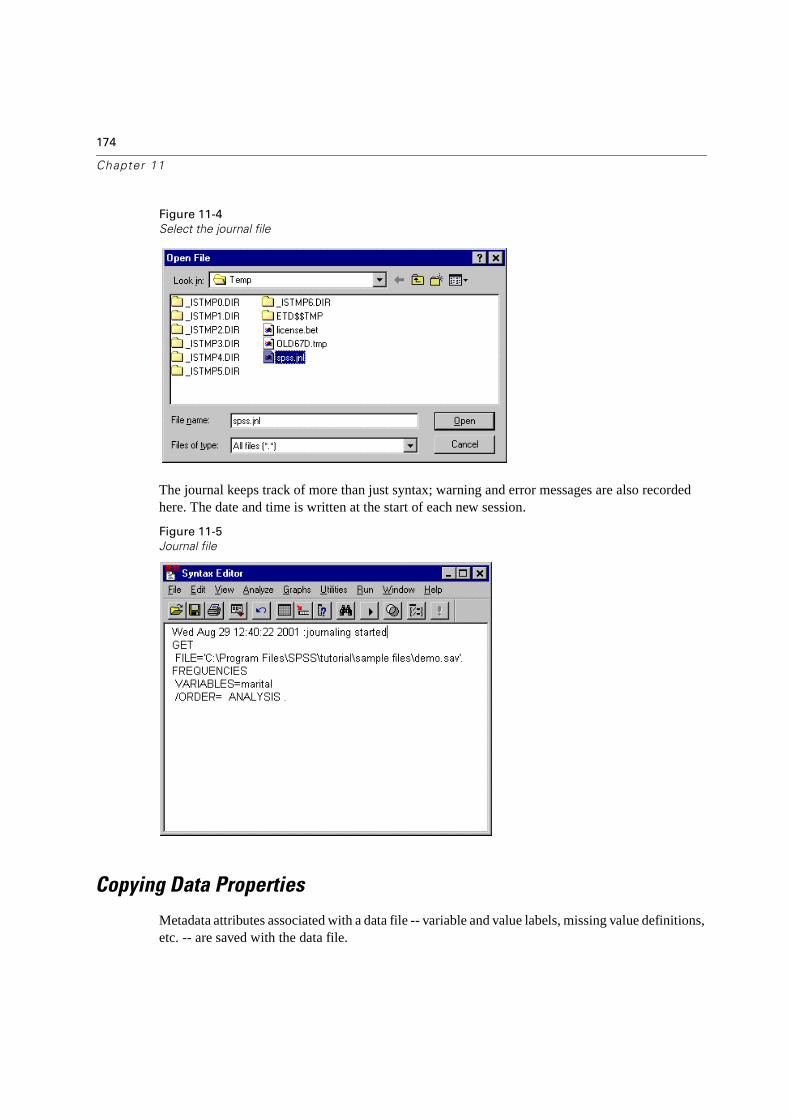
174
Chapter 11
Figure 11-4
Select the journal file
The journal keeps track of more than just syntax; warning and error messages are also recorded here. The date and time is written at the start of each new session.
Figure 11-5
Journal file
Copying Data Properties
Metadata attributes associated with a data file -- variable and value labels, missing value definitions, etc. -- are saved with the data file.
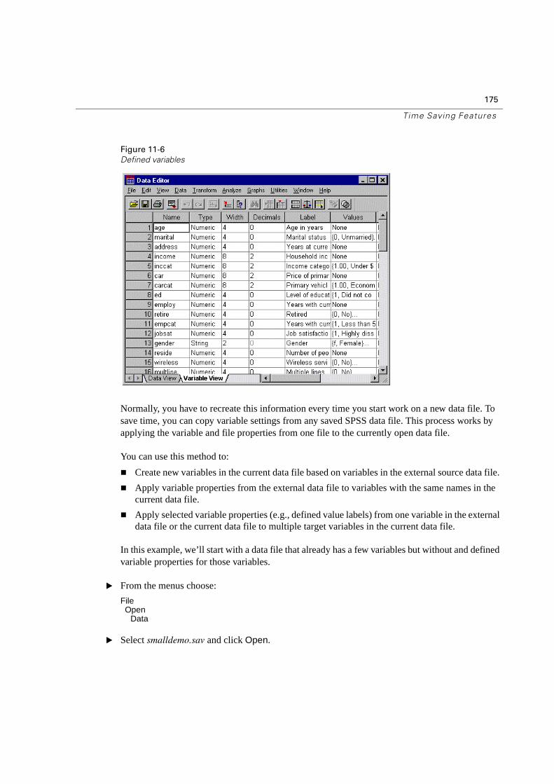
175
Time Saving Features
Figure 11-6
Defined variables
Normally, you have to recreate this information every time you start work on a new data file. To save time, you can copy variable settings from any saved SPSS data file. This process works by applying the variable and file properties from one file to the currently open data file.
You can use this method to:
� Create new variables in the current data file based on variables in the external source data file.
� Apply variable properties from the external data file to variables with the same names in the current data file.
� Apply selected variable properties (e.g., defined value labels) from one variable in the external data file or the current data file to multiple target variables in the current data file.
In this example, we’ll start with a data file that already has a few variables but without and defined variable properties for those variables.
� From the menus choose:
FileOpen
Data
� Select smalldemo.sav and click Open.
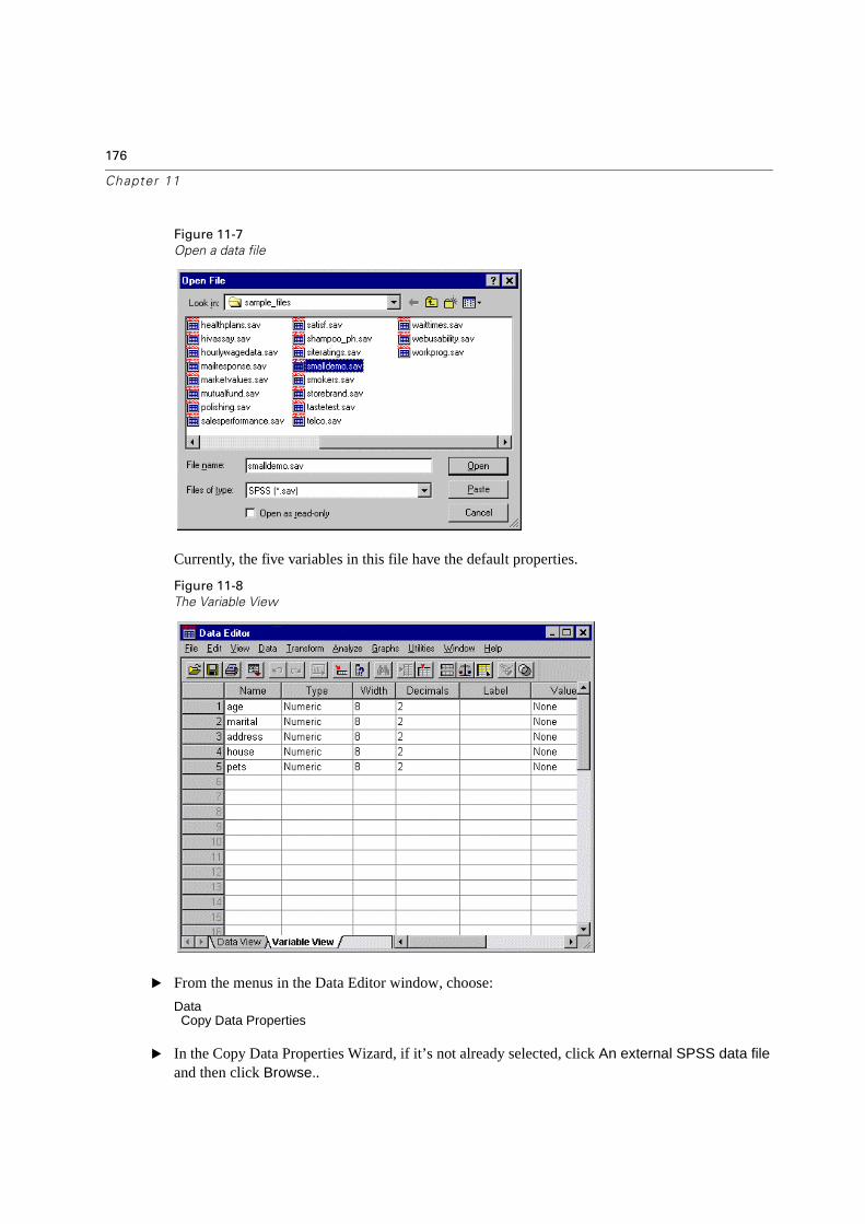
176
Chapter 11
Figure 11-7
Open a data file
Currently, the five variables in this file have the default properties.
Figure 11-8
The Variable View
� From the menus in the Data Editor window, choose:
DataCopy Data Properties
� In the Copy Data Properties Wizard, if it’s not already selected, click An external SPSS data fileand then click Browse..
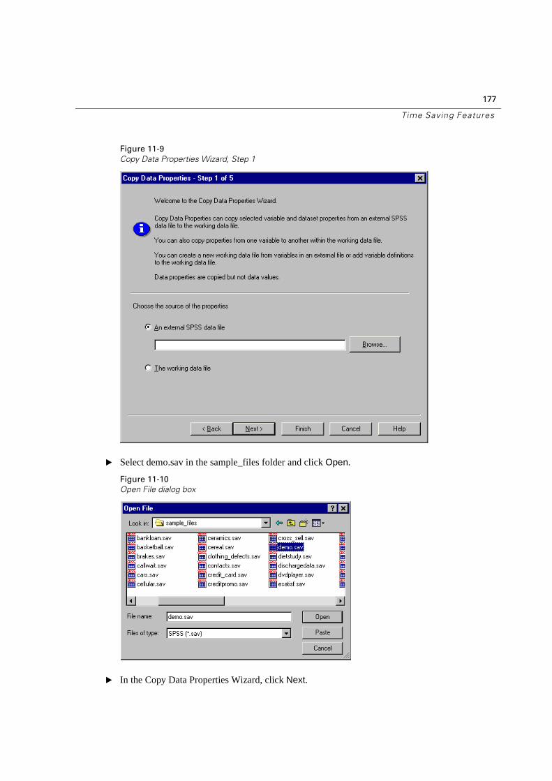
177
Time Saving Features
Figure 11-9
Copy Data Properties Wizard, Step 1
� Select demo.sav in the sample_files folder and click Open.
Figure 11-10
Open File dialog box
� In the Copy Data Properties Wizard, click Next.
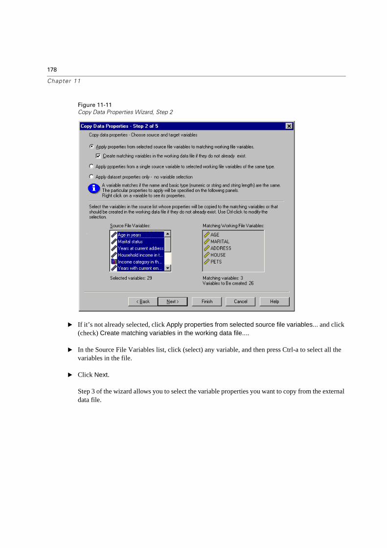
178
Chapter 11
Figure 11-11
Copy Data Properties Wizard, Step 2
� If it’s not already selected, click Apply properties from selected source file variables... and click (check) Create matching variables in the working data file....
� In the Source File Variables list, click (select) any variable, and then press Ctrl-a to select all the variables in the file.
� Click Next.
Step 3 of the wizard allows you to select the variable properties you want to copy from the external data file.

179
Time Saving Features
Figure 11-12
Copy Data Properties Wizard, Step 3, variable properties
For matching variables in the two files (variables with the same name and type), you can either Replace or Merge value labels. If the working data file had any defined value labels, the Replace option would delete all the existing value labels for matching variables and replace them with the labels from the matching variable in the external data file. In this example, however, there are no defined value labels; so there’s no difference between Replace and Merge.
� Click Finish to run the wizard and copy the variable properties from the external source file to the current data file.
� Make the Data Editor the active window and, if Variable View isn’t already displayed, click the Variable View tab.
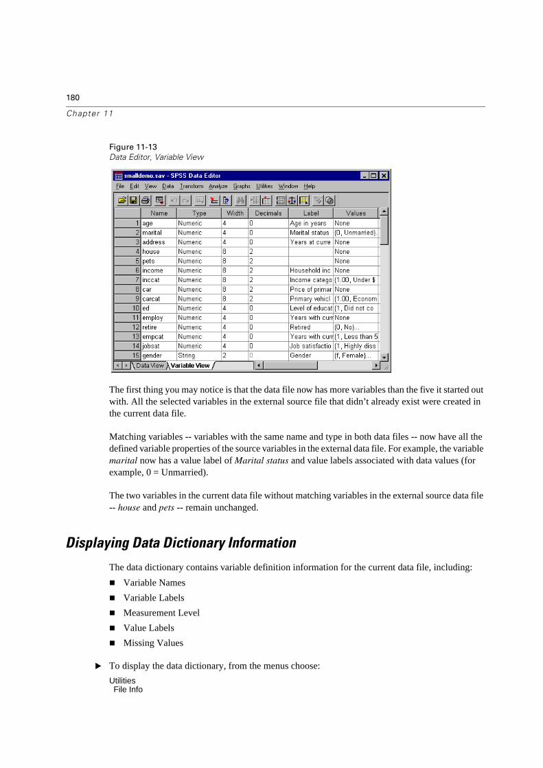
180
Chapter 11
Figure 11-13
Data Editor, Variable View
The first thing you may notice is that the data file now has more variables than the five it started out with. All the selected variables in the external source file that didn’t already exist were created in the current data file.
Matching variables -- variables with the same name and type in both data files -- now have all the defined variable properties of the source variables in the external data file. For example, the variable marital now has a value label of Marital status and value labels associated with data values (for example, 0 = Unmarried).
The two variables in the current data file without matching variables in the external source data file -- house and pets -- remain unchanged.
Displaying Data Dictionary Information
The data dictionary contains variable definition information for the current data file, including:
� Variable Names
� Variable Labels
� Measurement Level
� Value Labels
� Missing Values
� To display the data dictionary, from the menus choose:
UtilitiesFile Info
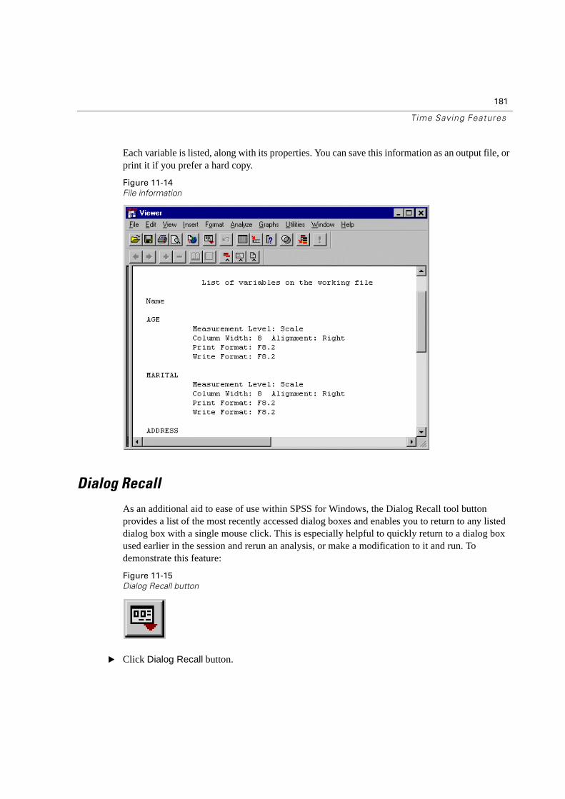
181
Time Saving Features
Each variable is listed, along with its properties. You can save this information as an output file, or print it if you prefer a hard copy.
Figure 11-14
File information
Dialog Recall
As an additional aid to ease of use within SPSS for Windows, the Dialog Recall tool button provides a list of the most recently accessed dialog boxes and enables you to return to any listed dialog box with a single mouse click. This is especially helpful to quickly return to a dialog box used earlier in the session and rerun an analysis, or make a modification to it and run. To demonstrate this feature:
Figure 11-15
Dialog Recall button
� Click Dialog Recall button.
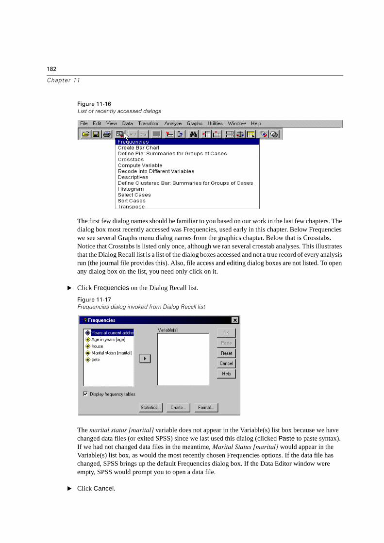
182
Chapter 11
Figure 11-16
List of recently accessed dialogs
The first few dialog names should be familiar to you based on our work in the last few chapters. The dialog box most recently accessed was Frequencies, used early in this chapter. Below Frequencies we see several Graphs menu dialog names from the graphics chapter. Below that is Crosstabs. Notice that Crosstabs is listed only once, although we ran several crosstab analyses. This illustrates that the Dialog Recall list is a list of the dialog boxes accessed and not a true record of every analysis run (the journal file provides this). Also, file access and editing dialog boxes are not listed. To open any dialog box on the list, you need only click on it.
� Click Frequencies on the Dialog Recall list.
Figure 11-17
Frequencies dialog invoked from Dialog Recall list
The marital status [marital] variable does not appear in the Variable(s) list box because we have changed data files (or exited SPSS) since we last used this dialog (clicked Paste to paste syntax). If we had not changed data files in the meantime, Marital Status [marital] would appear in the Variable(s) list box, as would the most recently chosen Frequencies options. If the data file has changed, SPSS brings up the default Frequencies dialog box. If the Data Editor window were empty, SPSS would prompt you to open a data file.
� Click Cancel.
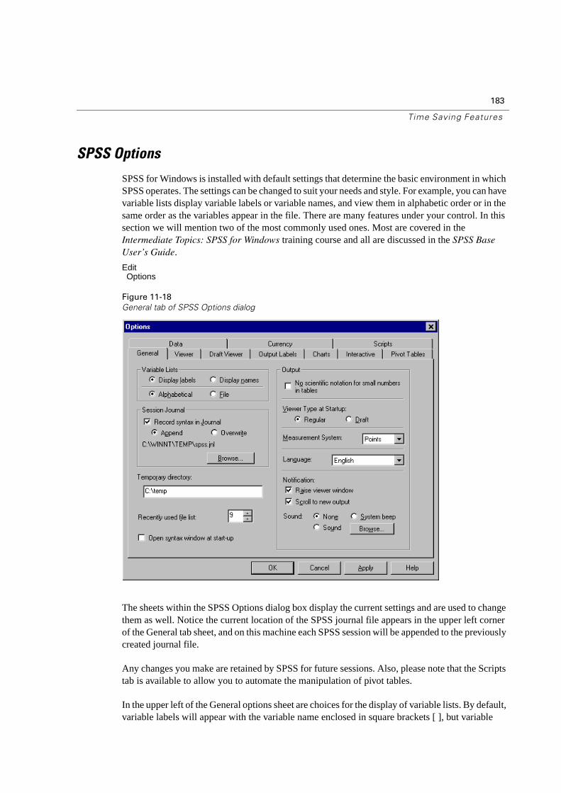
183
Time Saving Features
SPSS Options
SPSS for Windows is installed with default settings that determine the basic environment in which SPSS operates. The settings can be changed to suit your needs and style. For example, you can have variable lists display variable labels or variable names, and view them in alphabetic order or in the same order as the variables appear in the file. There are many features under your control. In this section we will mention two of the most commonly used ones. Most are covered in the Intermediate Topics: SPSS for Windows training course and all are discussed in the SPSS Base
User’s Guide.
EditOptions
Figure 11-18
General tab of SPSS Options dialog
The sheets within the SPSS Options dialog box display the current settings and are used to change them as well. Notice the current location of the SPSS journal file appears in the upper left corner of the General tab sheet, and on this machine each SPSS session will be appended to the previously created journal file.
Any changes you make are retained by SPSS for future sessions. Also, please note that the Scripts tab is available to allow you to automate the manipulation of pivot tables.
In the upper left of the General options sheet are choices for the display of variable lists. By default, variable labels will appear with the variable name enclosed in square brackets [ ], but variable
184
Chapter 11
names alone can be chosen. For display order the default is file order. This might be preferred if data come from a spreadsheet and analysts like to retain the original column order when SPSS lists the variables in dialog boxes. Also, for survey data in which the variables are named Q1, Q2a, Q2b, Q3, etc., the order of the variables in the file (File order) is more convenient. Alphabetical order is preferred if the variable names (or labels) are recognizable, since it makes it easier to locate the variables by name (or label). To change either variable list option, simply click the appropriate option button, then click Apply or OK.
A second aspect often modified is the TableLook discussed in the "Working with Output" chapter. Clicking on the Pivot Tables tab will lead you to formatting features that can be applied to pivot tables. You control such pivot table attributes as grid lines, fonts and colors.
This is a very brief look at the SPSS Options dialog box. Yet it serves to make the point that the Options dialog box gives you control over the SPSS environment. It is worth your time to investigate it further.
� Click Cancel.
185
Chapte r
12Multiple Response Variables
Introduction to Multiple Response Variables
We discuss a procedure in SPSS designed to produce frequency and crosstab tables when several responses can be made (or recorded) to a single question. Other SPSS procedures treat each variable as a separate entity; the Multiple Response procedure combines multiple variables measuring the same thing into a single table. We will show you how to set up such analyses and discuss the choices you have in requesting percentage summaries. The Multiple Response procedure is part of the SPSS Base System. If you have the SPSS Tables option, it too can accept multiple response variables, but it provides much greater format control and supports far more complex summary table organization.
What are Multiple Response Variables?
There are data collection situations in which several responses or measurements are recorded for a single question. For example, people might be asked to list every airline they have flown in the last six months, or to name every magazine to which they subscribe. In quality control applications all defects found in a sampled product might be recorded, or there might be a list of product characteristics, each one of which is checked if it is found to be within specification limits. When measuring customer satisfaction, you might ask those surveyed to tell you what they like and what they don’t like about your product or service. In this chapter we review the Multiple Response procedure in SPSS that produces summary frequency and crosstabulation tables composed of such multiple response variables.
There are questions of this type in the General Social Survey. Respondents were asked to name the most important problems they (and members of their household) had during the last twelve months. Up to four responses were recorded and stored in the variables prob1 to prob4. In this situation the survey designers expect each respondent to name, at most, a few of their most important problems. This is the rationale for recording the information in only four variables. Such common survey questions as "Tell me what you like (or dislike) about product X" are of this type. The coding scheme for the General Social Survey prob1 to prob4 variables appears below.
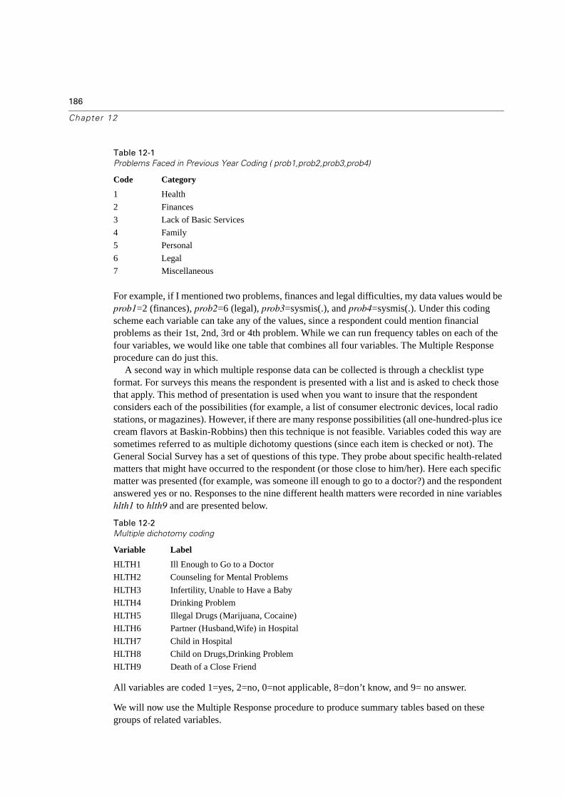
186
Chapter 12
Table 12-1
Problems Faced in Previous Year Coding ( prob1,prob2,prob3,prob4)
For example, if I mentioned two problems, finances and legal difficulties, my data values would be prob1=2 (finances), prob2=6 (legal), prob3=sysmis(.), and prob4=sysmis(.). Under this coding scheme each variable can take any of the values, since a respondent could mention financial problems as their 1st, 2nd, 3rd or 4th problem. While we can run frequency tables on each of the four variables, we would like one table that combines all four variables. The Multiple Response procedure can do just this.
A second way in which multiple response data can be collected is through a checklist type format. For surveys this means the respondent is presented with a list and is asked to check those that apply. This method of presentation is used when you want to insure that the respondent considers each of the possibilities (for example, a list of consumer electronic devices, local radio stations, or magazines). However, if there are many response possibilities (all one-hundred-plus ice cream flavors at Baskin-Robbins) then this technique is not feasible. Variables coded this way are sometimes referred to as multiple dichotomy questions (since each item is checked or not). The General Social Survey has a set of questions of this type. They probe about specific health-related matters that might have occurred to the respondent (or those close to him/her). Here each specific matter was presented (for example, was someone ill enough to go to a doctor?) and the respondent answered yes or no. Responses to the nine different health matters were recorded in nine variables hlth1 to hlth9 and are presented below.
Table 12-2
Multiple dichotomy coding
All variables are coded 1=yes, 2=no, 0=not applicable, 8=don’t know, and 9= no answer.
We will now use the Multiple Response procedure to produce summary tables based on these groups of related variables.
Code Category
1 Health
2 Finances
3 Lack of Basic Services
4 Family
5 Personal
6 Legal
7 Miscellaneous
Variable Label
HLTH1 Ill Enough to Go to a Doctor
HLTH2 Counseling for Mental Problems
HLTH3 Infertility, Unable to Have a Baby
HLTH4 Drinking Problem
HLTH5 Illegal Drugs (Marijuana, Cocaine)
HLTH6 Partner (Husband,Wife) in Hospital
HLTH7 Child in Hospital
HLTH8 Child on Drugs,Drinking Problem
HLTH9 Death of a Close Friend
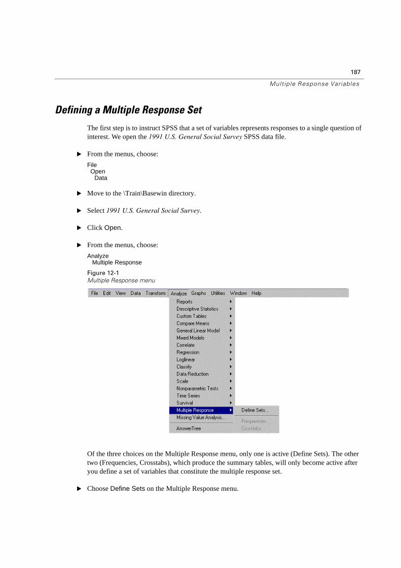
187
Multiple Response Variables
Defining a Multiple Response Set
The first step is to instruct SPSS that a set of variables represents responses to a single question of interest. We open the 1991 U.S. General Social Survey SPSS data file.
� From the menus, choose:
FileOpen
Data
� Move to the \Train\Basewin directory.
� Select 1991 U.S. General Social Survey.
� Click Open.
� From the menus, choose:
Analyze Multiple Response
Figure 12-1
Multiple Response menu
Of the three choices on the Multiple Response menu, only one is active (Define Sets). The other two (Frequencies, Crosstabs), which produce the summary tables, will only become active after you define a set of variables that constitute the multiple response set.
� Choose Define Sets on the Multiple Response menu.
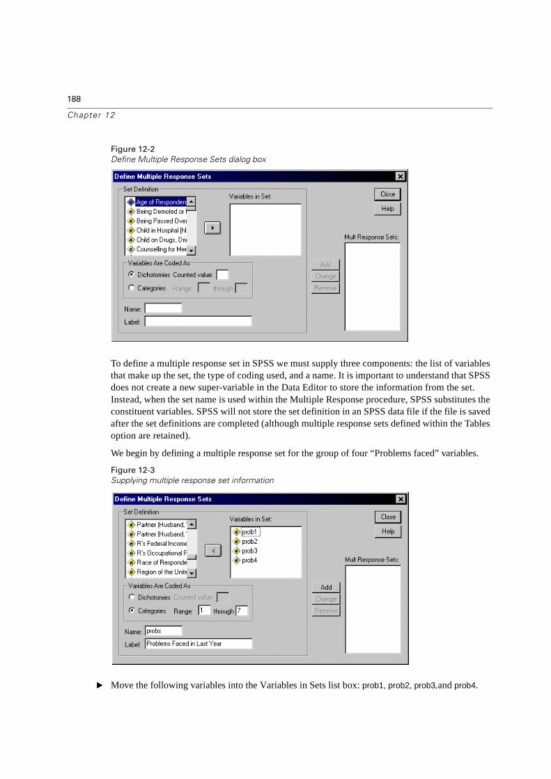
188
Chapter 12
Figure 12-2
Define Multiple Response Sets dialog box
To define a multiple response set in SPSS we must supply three components: the list of variables that make up the set, the type of coding used, and a name. It is important to understand that SPSS does not create a new super-variable in the Data Editor to store the information from the set. Instead, when the set name is used within the Multiple Response procedure, SPSS substitutes the constituent variables. SPSS will not store the set definition in an SPSS data file if the file is saved after the set definitions are completed (although multiple response sets defined within the Tables option are retained).
We begin by defining a multiple response set for the group of four “Problems faced” variables.
Figure 12-3
Supplying multiple response set information
� Move the following variables into the Variables in Sets list box: prob1, prob2, prob3,and prob4.
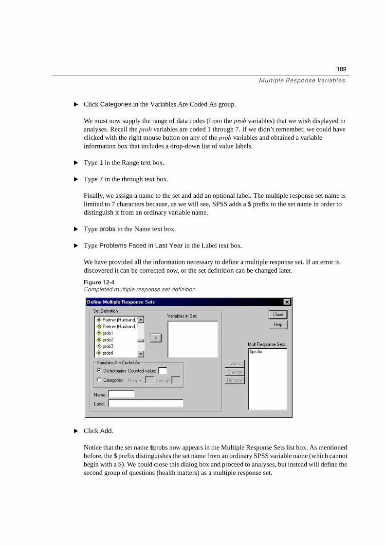
189
Multiple Response Variables
� Click Categories in the Variables Are Coded As group.
We must now supply the range of data codes (from the prob variables) that we wish displayed in analyses. Recall the prob variables are coded 1 through 7. If we didn’t remember, we could have clicked with the right mouse button on any of the prob variables and obtained a variable information box that includes a drop-down list of value labels.
� Type 1 in the Range text box.
� Type 7 in the through text box.
Finally, we assign a name to the set and add an optional label. The multiple response set name is limited to 7 characters because, as we will see, SPSS adds a $ prefix to the set name in order to distinguish it from an ordinary variable name.
� Type probs in the Name text box.
� Type Problems Faced in Last Year in the Label text box.
We have provided all the information necessary to define a multiple response set. If an error is discovered it can be corrected now, or the set definition can be changed later.
Figure 12-4
Completed multiple response set definition
� Click Add.
Notice that the set name $probs now appears in the Multiple Response Sets list box. As mentioned before, the $ prefix distinguishes the set name from an ordinary SPSS variable name (which cannot begin with a $). We could close this dialog box and proceed to analyses, but instead will define the second group of questions (health matters) as a multiple response set.
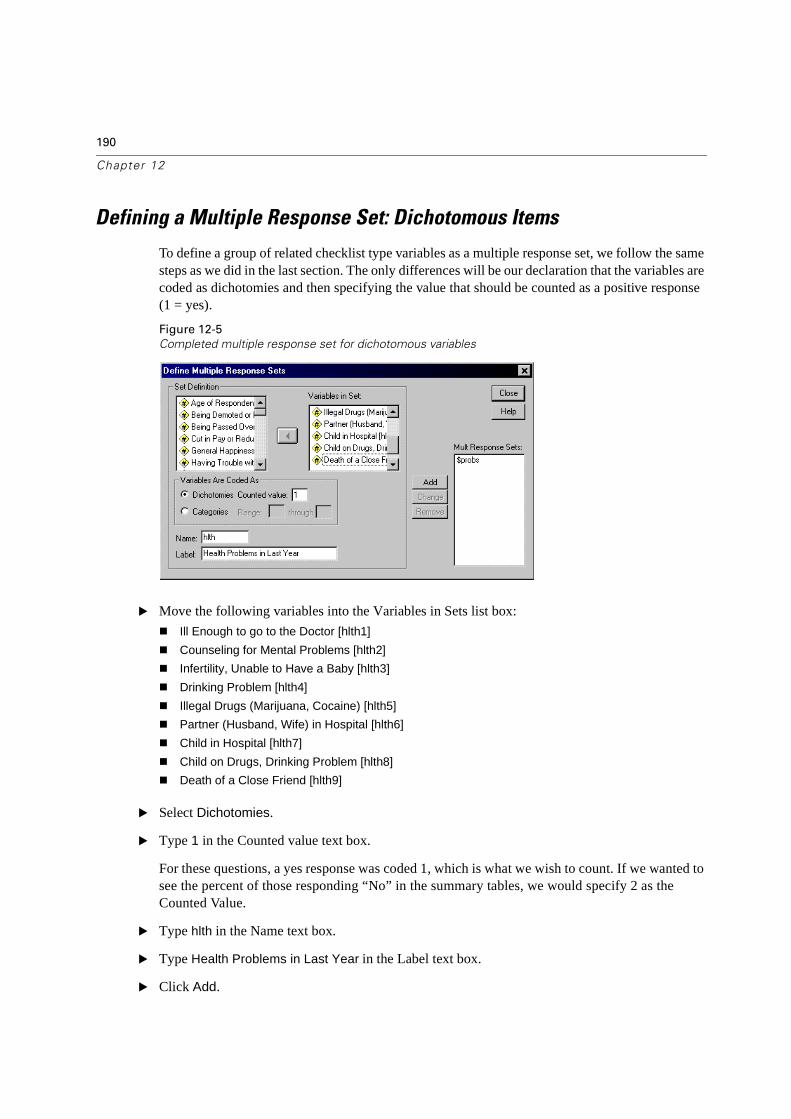
190
Chapter 12
Defining a Multiple Response Set: Dichotomous Items
To define a group of related checklist type variables as a multiple response set, we follow the same steps as we did in the last section. The only differences will be our declaration that the variables are coded as dichotomies and then specifying the value that should be counted as a positive response (1 = yes).
Figure 12-5
Completed multiple response set for dichotomous variables
� Move the following variables into the Variables in Sets list box:
� Ill Enough to go to the Doctor [hlth1]
� Counseling for Mental Problems [hlth2]
� Infertility, Unable to Have a Baby [hlth3]
� Drinking Problem [hlth4]
� Illegal Drugs (Marijuana, Cocaine) [hlth5]
� Partner (Husband, Wife) in Hospital [hlth6]
� Child in Hospital [hlth7]
� Child on Drugs, Drinking Problem [hlth8]
� Death of a Close Friend [hlth9]
� Select Dichotomies.
� Type 1 in the Counted value text box.
For these questions, a yes response was coded 1, which is what we wish to count. If we wanted to see the percent of those responding “No” in the summary tables, we would specify 2 as the Counted Value.
� Type hlth in the Name text box.
� Type Health Problems in Last Year in the Label text box.
� Click Add.
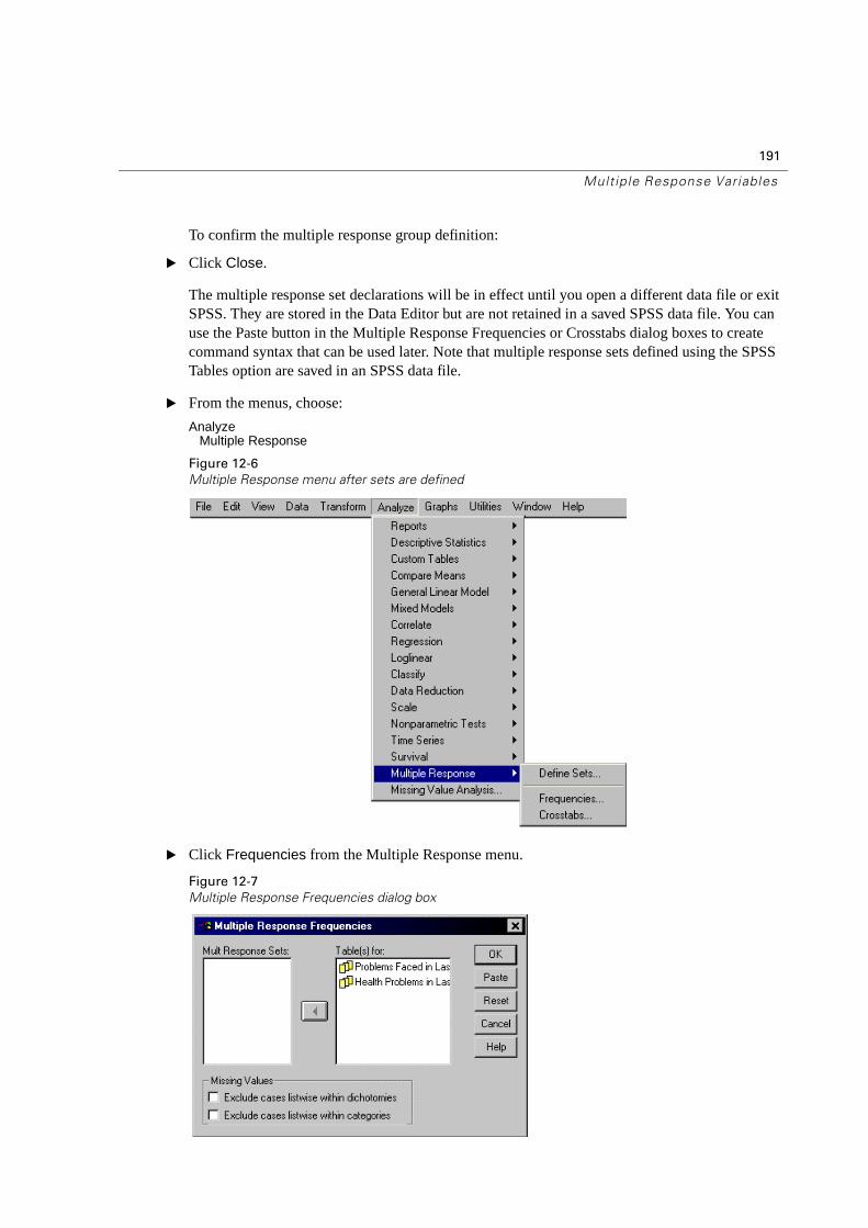
191
Multiple Response Variables
To confirm the multiple response group definition:
� Click Close.
The multiple response set declarations will be in effect until you open a different data file or exit SPSS. They are stored in the Data Editor but are not retained in a saved SPSS data file. You can use the Paste button in the Multiple Response Frequencies or Crosstabs dialog boxes to create command syntax that can be used later. Note that multiple response sets defined using the SPSS Tables option are saved in an SPSS data file.
� From the menus, choose:
Analyze Multiple Response
Figure 12-6
Multiple Response menu after sets are defined
� Click Frequencies from the Multiple Response menu.
Figure 12-7
Multiple Response Frequencies dialog box
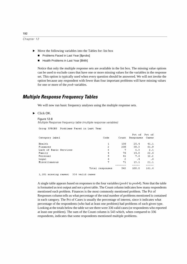
192
Chapter 12
� Move the following variables into the Tables for: list box
� Problems Faced in Last Year [$probs]
� Health Problems in Last Year [$hlth]
Notice that only the multiple response sets are available in the list box. The missing value options can be used to exclude cases that have one or more missing values for the variables in the response set. This option is typically used when every question should be answered. We will not invoke the option because any respondent with fewer than four important problems will have missing values for one or more of the prob variables.
Multiple Response Frequency Tables
We will now run basic frequency analyses using the multiple response sets.
� Click OK.
Figure 12-8
Multiple Response frequency table (multiple response variables)
A single table appears based on responses to the four variables (prob1 to prob4). Note that the table is formatted as text output and not a pivot table. The Count column indicates how many respondents mentioned each problem. Finances is the most commonly mentioned problem. The Pct of Responses column tells us what percentage of the total number of problems mentioned is contained in each category. The Pct of Cases is usually the percentage of interest, since it indicates what percentage of the respondents (who had at least one problem) had problems of each given type. Looking at the totals below the table we see there were 336 valid cases (or respondents who reported at least one problem). The sum of the Count column is 543 which, when compared to 336 respondents, indicates that some respondents mentioned multiple problems.
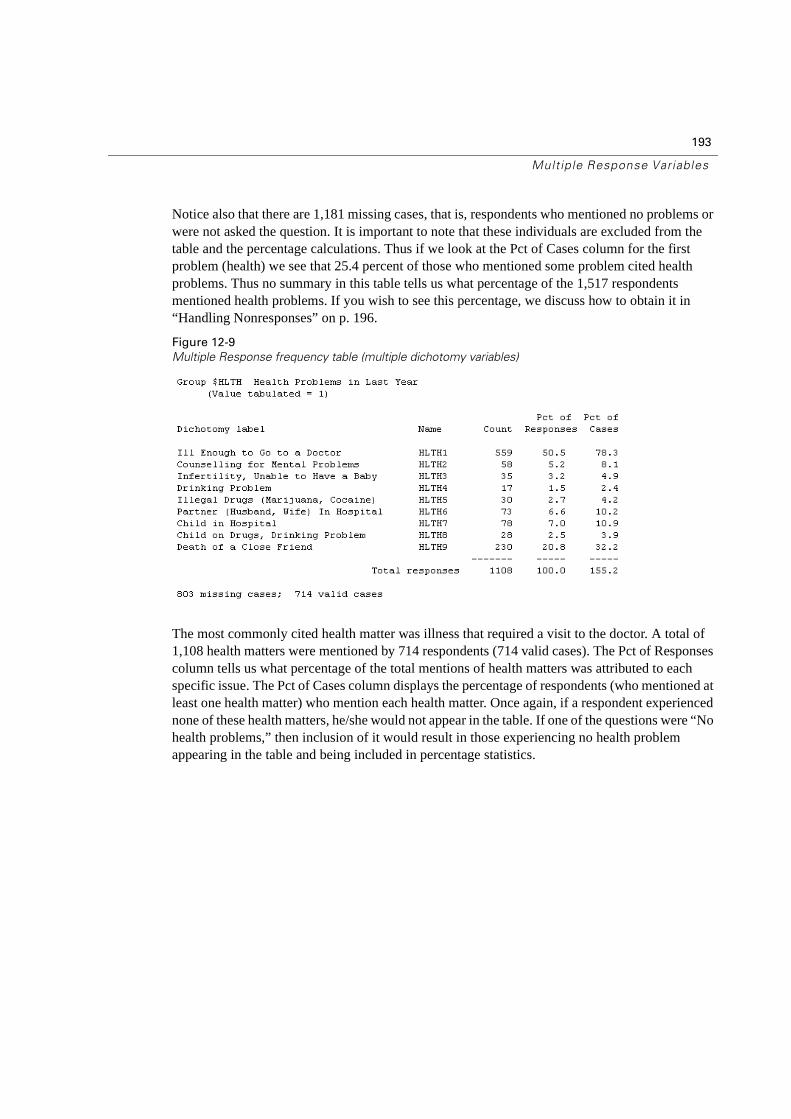
193
Multiple Response Variables
Notice also that there are 1,181 missing cases, that is, respondents who mentioned no problems or were not asked the question. It is important to note that these individuals are excluded from the table and the percentage calculations. Thus if we look at the Pct of Cases column for the first problem (health) we see that 25.4 percent of those who mentioned some problem cited health problems. Thus no summary in this table tells us what percentage of the 1,517 respondents mentioned health problems. If you wish to see this percentage, we discuss how to obtain it in “Handling Nonresponses” on p. 196.
Figure 12-9
Multiple Response frequency table (multiple dichotomy variables)
The most commonly cited health matter was illness that required a visit to the doctor. A total of 1,108 health matters were mentioned by 714 respondents (714 valid cases). The Pct of Responses column tells us what percentage of the total mentions of health matters was attributed to each specific issue. The Pct of Cases column displays the percentage of respondents (who mentioned at least one health matter) who mention each health matter. Once again, if a respondent experienced none of these health matters, he/she would not appear in the table. If one of the questions were “Nohealth problems,” then inclusion of it would result in those experiencing no health problem appearing in the table and being included in percentage statistics.
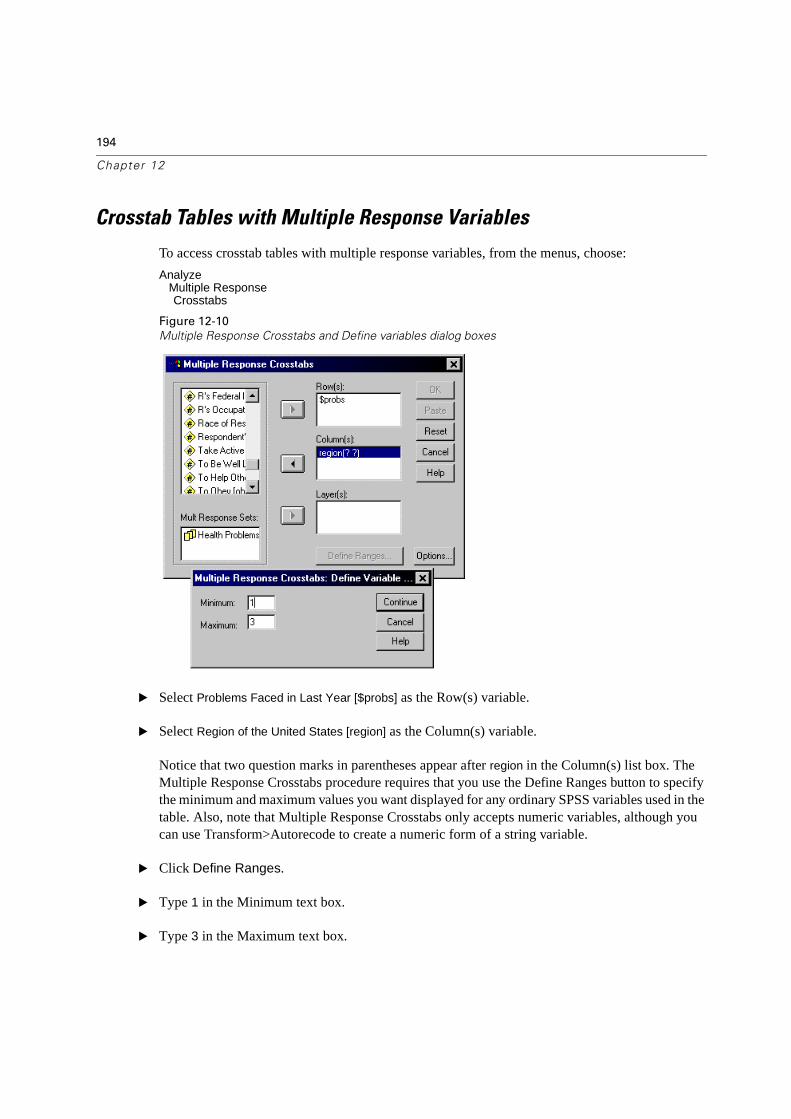
194
Chapter 12
Crosstab Tables with Multiple Response Variables
To access crosstab tables with multiple response variables, from the menus, choose:
Analyze Multiple Response
Crosstabs
Figure 12-10
Multiple Response Crosstabs and Define variables dialog boxes
� Select Problems Faced in Last Year [$probs] as the Row(s) variable.
� Select Region of the United States [region] as the Column(s) variable.
Notice that two question marks in parentheses appear after region in the Column(s) list box. The Multiple Response Crosstabs procedure requires that you use the Define Ranges button to specify the minimum and maximum values you want displayed for any ordinary SPSS variables used in the table. Also, note that Multiple Response Crosstabs only accepts numeric variables, although you can use Transform>Autorecode to create a numeric form of a string variable.
� Click Define Ranges.
� Type 1 in the Minimum text box.
� Type 3 in the Maximum text box.
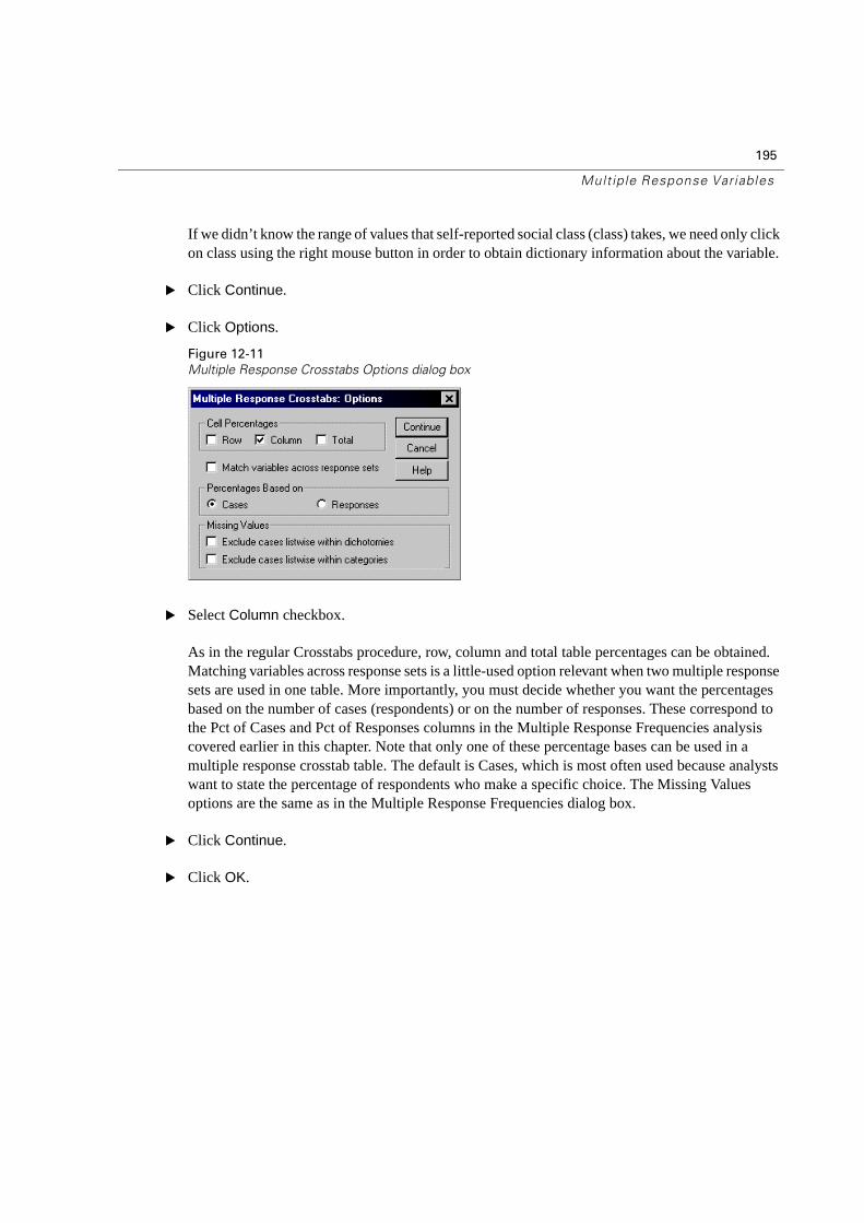
195
Multiple Response Variables
If we didn’t know the range of values that self-reported social class (class) takes, we need only click on class using the right mouse button in order to obtain dictionary information about the variable.
� Click Continue.
� Click Options.
Figure 12-11
Multiple Response Crosstabs Options dialog box
� Select Column checkbox.
As in the regular Crosstabs procedure, row, column and total table percentages can be obtained. Matching variables across response sets is a little-used option relevant when two multiple response sets are used in one table. More importantly, you must decide whether you want the percentages based on the number of cases (respondents) or on the number of responses. These correspond to the Pct of Cases and Pct of Responses columns in the Multiple Response Frequencies analysis covered earlier in this chapter. Note that only one of these percentage bases can be used in a multiple response crosstab table. The default is Cases, which is most often used because analysts want to state the percentage of respondents who make a specific choice. The Missing Values options are the same as in the Multiple Response Frequencies dialog box.
� Click Continue.
� Click OK.
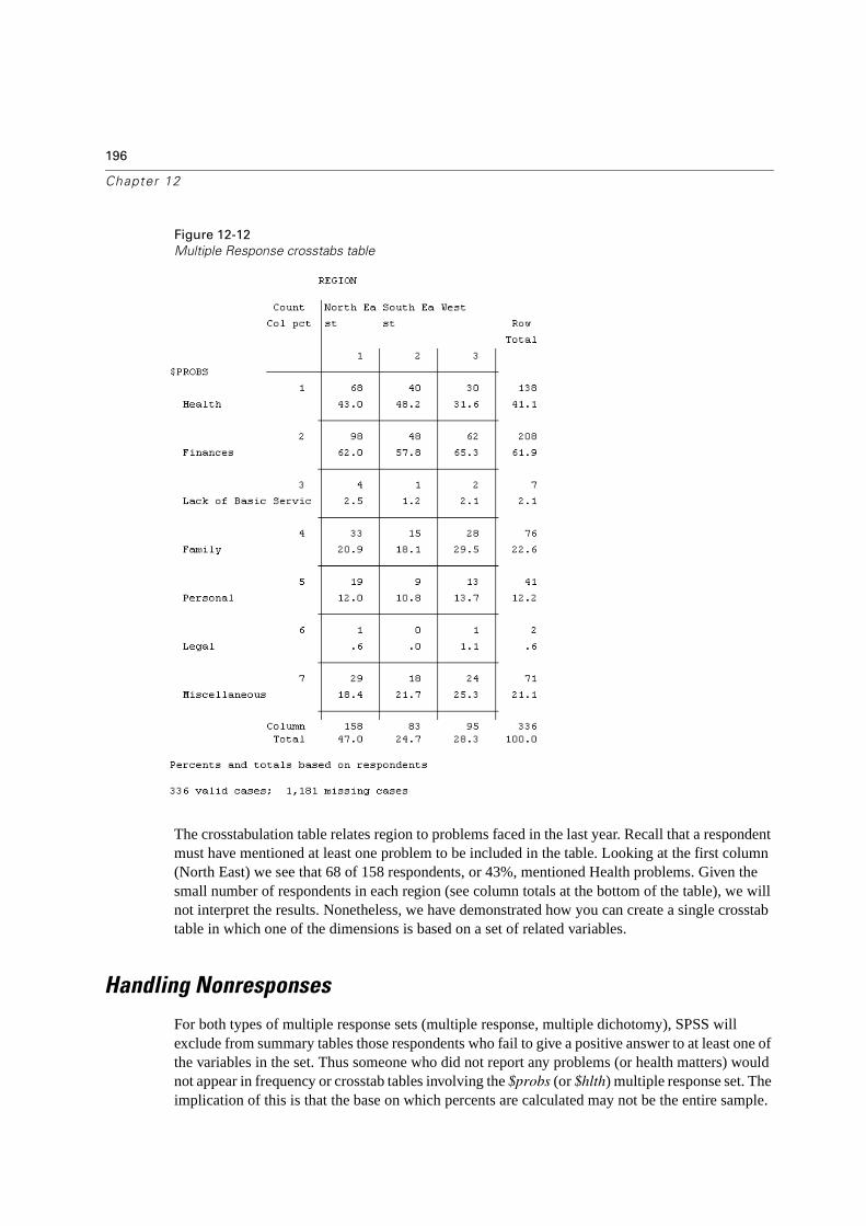
196
Chapter 12
Figure 12-12
Multiple Response crosstabs table
The crosstabulation table relates region to problems faced in the last year. Recall that a respondent must have mentioned at least one problem to be included in the table. Looking at the first column (North East) we see that 68 of 158 respondents, or 43%, mentioned Health problems. Given the small number of respondents in each region (see column totals at the bottom of the table), we will not interpret the results. Nonetheless, we have demonstrated how you can create a single crosstab table in which one of the dimensions is based on a set of related variables.
Handling Nonresponses
For both types of multiple response sets (multiple response, multiple dichotomy), SPSS will exclude from summary tables those respondents who fail to give a positive answer to at least one of the variables in the set. Thus someone who did not report any problems (or health matters) would not appear in frequency or crosstab tables involving the $probs (or $hlth) multiple response set. The implication of this is that the base on which percents are calculated may not be the entire sample.
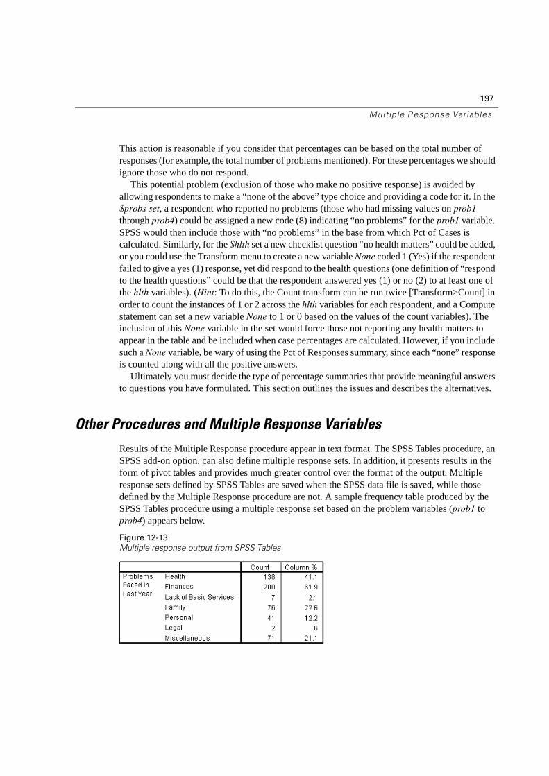
197
Multiple Response Variables
This action is reasonable if you consider that percentages can be based on the total number of responses (for example, the total number of problems mentioned). For these percentages we should ignore those who do not respond.
This potential problem (exclusion of those who make no positive response) is avoided by allowing respondents to make a “none of the above” type choice and providing a code for it. In the $probs set, a respondent who reported no problems (those who had missing values on prob1
through prob4) could be assigned a new code (8) indicating “no problems” for the prob1 variable. SPSS would then include those with “no problems” in the base from which Pct of Cases is calculated. Similarly, for the $hlth set a new checklist question “no health matters” could be added, or you could use the Transform menu to create a new variable None coded 1 (Yes) if the respondent failed to give a yes (1) response, yet did respond to the health questions (one definition of “respond to the health questions” could be that the respondent answered yes (1) or no (2) to at least one of the hlth variables). (Hint: To do this, the Count transform can be run twice [Transform>Count] in order to count the instances of 1 or 2 across the hlth variables for each respondent, and a Compute statement can set a new variable None to 1 or 0 based on the values of the count variables). The inclusion of this None variable in the set would force those not reporting any health matters to appear in the table and be included when case percentages are calculated. However, if you include such a None variable, be wary of using the Pct of Responses summary, since each “none” response is counted along with all the positive answers.
Ultimately you must decide the type of percentage summaries that provide meaningful answers to questions you have formulated. This section outlines the issues and describes the alternatives.
Other Procedures and Multiple Response Variables
Results of the Multiple Response procedure appear in text format. The SPSS Tables procedure, an SPSS add-on option, can also define multiple response sets. In addition, it presents results in the form of pivot tables and provides much greater control over the format of the output. Multiple response sets defined by SPSS Tables are saved when the SPSS data file is saved, while those defined by the Multiple Response procedure are not. A sample frequency table produced by the SPSS Tables procedure using a multiple response set based on the problem variables (prob1 to prob4) appears below.
Figure 12-13
Multiple response output from SPSS Tables

198
Chapter 12
Summary
We reviewed the Multiple Response procedure, which is used to create a single summary table of counts and percents, based on several variables that contain responses to one question.
199
Chapte r
13Hands-On Exercises
Background for the Bank Data File
The data file used for exercises contains demographic, salary and job information on the employees of a Midwestern bank around 1965. We are interested in understanding the employees in terms of demographics (gender, minority status, education) and employment measures (job position and beginning salary). In addition, we want to look at relations between demographics and beginning salary. Finally we want to represent our findings graphically. You are not expected to perform the definitive study on this data, but rather make a start in terms of describing these people and take a preliminary look at how the measures interrelate.
The data are stored in several file formats (including a fixed column text file). In the course of performing the exercises you will read this data, supply labels and missing values, perform several statistical analyses, modify the data, and create several charts.
Some of the exercises are marked For those with extra time. If you have completed the regular exercises and wish to try some advanced variations, please avail yourself of them. It is not necessary to perform these advanced exercises in order to fulfill the goals of this course.
Data Location
All data files, unless otherwise noted, are located in the directory \Train\Basewin. They should be copied from the 3.5 floppy disk or CD accompanying the Training guide to this directory if you are not working at an SPSS training site.
Using the Help System
This exercise does not involve the bank study per se, but explores the Help system within SPSS for Windows.
� To start SPSS for Windows, from the menus choose:
StartPrograms
SPSS for WindowsSPSS for Windows
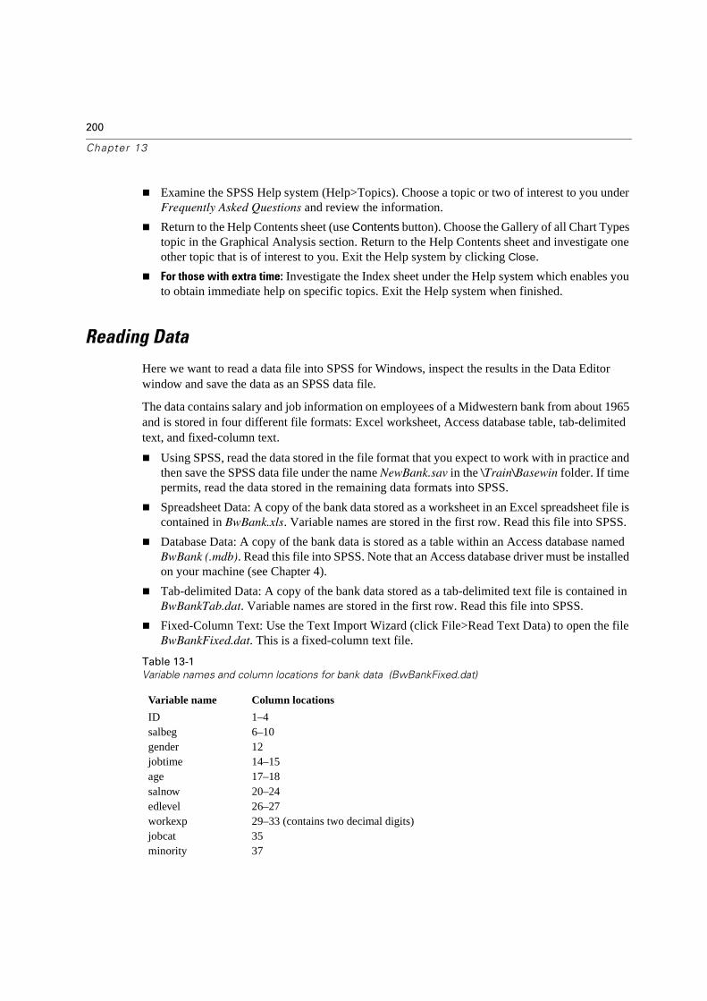
200
Chapter 13
� Examine the SPSS Help system (Help>Topics). Choose a topic or two of interest to you under Frequently Asked Questions and review the information.
� Return to the Help Contents sheet (use Contents button). Choose the Gallery of all Chart Types topic in the Graphical Analysis section. Return to the Help Contents sheet and investigate one other topic that is of interest to you. Exit the Help system by clicking Close.
� For those with extra time: Investigate the Index sheet under the Help system which enables you to obtain immediate help on specific topics. Exit the Help system when finished.
Reading Data
Here we want to read a data file into SPSS for Windows, inspect the results in the Data Editor window and save the data as an SPSS data file.
The data contains salary and job information on employees of a Midwestern bank from about 1965 and is stored in four different file formats: Excel worksheet, Access database table, tab-delimited text, and fixed-column text.
� Using SPSS, read the data stored in the file format that you expect to work with in practice and then save the SPSS data file under the name NewBank.sav in the \Train\Basewin folder. If time permits, read the data stored in the remaining data formats into SPSS.
� Spreadsheet Data: A copy of the bank data stored as a worksheet in an Excel spreadsheet file is contained in BwBank.xls. Variable names are stored in the first row. Read this file into SPSS.
� Database Data: A copy of the bank data is stored as a table within an Access database named BwBank (.mdb). Read this file into SPSS. Note that an Access database driver must be installed on your machine (see Chapter 4).
� Tab-delimited Data: A copy of the bank data stored as a tab-delimited text file is contained in BwBankTab.dat. Variable names are stored in the first row. Read this file into SPSS.
� Fixed-Column Text: Use the Text Import Wizard (click File>Read Text Data) to open the file BwBankFixed.dat. This is a fixed-column text file.
Table 13-1
Variable names and column locations for bank data (BwBankFixed.dat)
Variable name Column locations
ID 1–4salbeg 6–10gender 12jobtime 14–15age 17–18salnow 20–24edlevel 26–27workexp 29–33 (contains two decimal digits)jobcat 35minority 37
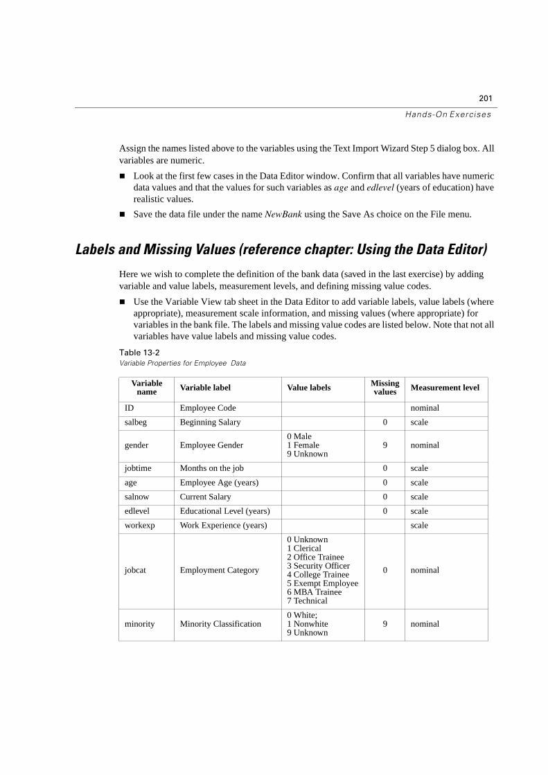
201
Hands-On Exercises
Assign the names listed above to the variables using the Text Import Wizard Step 5 dialog box. All variables are numeric.
� Look at the first few cases in the Data Editor window. Confirm that all variables have numeric data values and that the values for such variables as age and edlevel (years of education) have realistic values.
� Save the data file under the name NewBank using the Save As choice on the File menu.
Labels and Missing Values (reference chapter: Using the Data Editor)
Here we wish to complete the definition of the bank data (saved in the last exercise) by adding variable and value labels, measurement levels, and defining missing value codes.
� Use the Variable View tab sheet in the Data Editor to add variable labels, value labels (where appropriate), measurement scale information, and missing values (where appropriate) for variables in the bank file. The labels and missing value codes are listed below. Note that not all variables have value labels and missing value codes.
Table 13-2
Variable Properties for Employee Data
Variablename Variable label Value labels Missing
values Measurement level
ID Employee Code nominal
salbeg Beginning Salary 0 scale
gender Employee Gender0 Male 1 Female 9 Unknown
9 nominal
jobtime Months on the job 0 scale
age Employee Age (years) 0 scale
salnow Current Salary 0 scale
edlevel Educational Level (years) 0 scale
workexp Work Experience (years) scale
jobcat Employment Category
0 Unknown 1 Clerical 2 Office Trainee 3 Security Officer 4 College Trainee 5 Exempt Employee6 MBA Trainee 7 Technical
0 nominal
minority Minority Classification0 White; 1 Nonwhite9 Unknown
9 nominal
202
Chapter 13
� Run Frequencies on the labeled variables gender (employee gender) and jobcat (employment category).
� Save the file containing labels and missing values under the name NewBank (same as before) using the Save As choice from the File menu.
� For those with extra time: Add another case to the file to represent an employee of the bank in the mid-1960s. Save the file with this new case added.
Examining Summary Statistics for Individual Variables
In this exercise, we ask you to begin analyzing the bank data by producing some descriptive summaries on both the demographic and salary variables. These will provide summaries useful in describing the employees and serve as a check on the data values; for example, are the maximum and minimum values of education, age, and current salary reasonable?
� Open the SPSS data file NewBank (.sav), if you haven’t already done so.
� Run Frequencies on the variables jobcat (employment category), minority (minority classification), and gender (employee gender), requesting the mode, plus barcharts. Examine the bar charts to better understand the distributions of these variables. Which job category had the greatest number of employees and which had the fewest?
� Run Frequencies for salbeg (beginning salary) and salnow (current salary), requesting summary statistics, and a histogram for each variable with a superimposed normal curve. Suppress the display of the frequency table. Do you think that salaries are normally distributed? If not, why?
� For those with extra time: Produce a frequency distribution of edlevel (education level) showing the table in descending order of frequency (use the Format button).
Modifying Data Values
In this section, we will look at salary information in several different ways, which require some modification of the data. First we will group employees into several salary categories and see how many employees fall into each category. Next, we will study the difference between current and beginning salary across employees.
� Open the SPSS data file NewBank (.sav) if you haven’t already done so.
� Select Recode Into Different Variable from the Transform menu to create a new variable that groups salbeg (beginning salary) into six categories (call it salgrp). To decide which range of values to group together, you should look at the histogram or summary statistics from the exercise in Chapter 6. Alternatively, you can request Cut Points for 6 groups in the Percentile Values area under the Statistics button in the Frequencies dialog box to have SPSS provide endpoints for six approximately equal-sized groups. After the recode is complete, check your work by running frequencies of salgrp.
� UseCompute under the Transform menu to create a new variable that contains the difference between current and beginning salary (salnow and salbeg).
� Run Descriptives on this new variable, or run Frequencies requesting means while suppressing the frequency tables in order to see summary information. Can you tell whether anyone has a current salary lower than her beginning salary? What was the largest salary change?
203
Hands-On Exercises
� Save the modified data file as NewBank.
� For those with extra time: Use the variables jobtime (months on the job) and workexp (work experience) to create a new variable that measures the total time (in months) each employee has been working. You need to change workexp from years to months to do this. Examine summary information on this new variable.
� For those with even more extra time: Compute a new variable that divides the salary difference (see the third of this chapter’s exercises) by jobtime (months on the job). This will produce a salary difference adjusted for the number of months in the current job position. Run descriptive statistics on this new variable (use the Statistics button in the Frequencies dialog box or try the Descriptives procedure).
Crosstabulation Tables
Here we explore the relationships among gender, minority status and salary category (created in exercises from Chapter 7) using crosstabulation tables. Specifically, are there higher proportions of women falling in the lower salary categories.
� Run a crosstabulation table of the variables gender (employee gender) and minority (minority classification) (Analyze>Descriptive Statistics>Crosstabs).
� Create two crosstab tables of salgrp with each of the variables gender and minority. Display only column percentages. What is the relationship between salgrp and each of these variables?
� Produce a crosstab table of salgrp and gender with observed and expected counts. Request the chi-square statistic to test for a relationship.
� Save the Contents of the Viewer window (to the \Train\Basewin directory) under the name Exer8 (Exer8.spo).
� For those with extra time: Examine the relationship between gender and jobcat (employment category). Request appropriate statistics to test whether the two variables are independent. What is the expected number of female security officers? Then try constructing a three-way crosstab table of gender, minority, and salgrp (Hint: use salgrp as the row variable and minority
as the layer variable). Does the relationship between gender and salary differ by minority status?
Working with Output
We will modify the appearance of crosstab tables produced in the exercises for the Chapter 8. Open the Exer8(.spo) Viewer file created in the last exercise.
� Edit the pivot table for the second crosstab in the Contents pane (salgrp by gender with column percents). Transpose the Rows and Columns.
� Modify the width of the first column (containing value labels) until it seems best to you.
� Change the title to one that you feel provides a better description of the table.
� Apply several TableLooks to the table. Evaluate their strengths and weaknesses for the audience to whom you will be presenting your results.
204
Chapter 13
Creating and Editing Charts
Here we produce presentation charts that display the results of what we discovered running frequency and crosstab analyses earlier.
� Create a pie chart showing the distribution of jobcat (employment category) (use Graphs>Pie to create a standard graph). Add a title to the chart and display both the counts and labels.
� Produce a simple bar chart using either standard or Interactive graphs that displays the distribution of salary categories (salgrp).
� Create an Interactive graph that contains a clustered bar chart showing the distribution of salgrp
by gender. This displays the information appearing in the salgrp by gender crosstab table created in the exercises from Chapter 8.
� Change various aspects of the chart (orientation, fill color, fill pattern [style]). The quick method to begin is to double-click on the chart (which activates the Chart Editor).
� Create an Interactive graph that contains a scatterplot with beginning salary on the horizontal axis and current salary on the vertical axis.
� Save the contents of the Viewer window in the \Train\Basewin directory.
� For those with extra time: Create a clustered bar chart from the column percentages in the crosstab table produced in “Crosstabulation Tables” on p. 203.
� For those with extra time: Create a scatterplot of beginning salary and current salary again, then ask for a regression line to be drawn through the points (add an element). Next, try changing the tickmarks or range of the axes (Axis under the Format menu, or from Chart Manager).
Time Saving Features
These exercises do not directly advance the analysis of the bank data, but rather provide practice in features of SPSS that you will find useful.
� Open the NewBank (.sav) data file and create a pie chart based on job position. Open the SPSS.JNL file as a syntax window (File>Open>Syntax>All Files (*.*) on the Files of Type: drop-down list). Review the commands (near the bottom of the file if the journal option was set to append). Locate the syntax command (Graph) that ran the pie chart, select it and run it. Now return to the Syntax window, substitute the education variable for the job position variable and run the modified command.
� Click the Dialog Recall Box tool and review the SPSS dialog boxes recently accessed. Click on one of the choices. Why are no variables selected for analysis (from the previous use of the dialog box)?
� Display the codebook information for the NewBank (.sav) file by clicking Utilities>File Info. Verify that the labels and missing values you entered earlier are present.
Multiple Response Variables
This exercise uses the demo (.sav) file in the \tutorial\sample files directory, located in the SPSS installation directory.
205
Hands-On Exercises
Here we run additional analyses with multiple response variables, looking at the relation between telecom products and services owned and the marital status of the respondent. Each of the telecom product/service variables is coded 0 (not owned) or 1 (owned).
� Open the demo SPSS data file.
� Define a multiple response set (multiple dichotomy) called telprod for the set of questions asking about telecom products/services owned (it should include Call Waiting [callwait],
Caller ID [callid], Internet [internet], Multiple Lines [multline], Paging Service [pager],
Voice Mail [voice], Wireless Service [wireless]).
� Run a Multiple Response Frequency table of problems faced. Of the products/services mentioned, which appears least frequently?
� Create a Multiple Response Crosstab table of telprod by marital status (marital). Request column percentages based on cases. Does there seem to be any differences between the marital status groups in their use of telecom products or services?


207
I n d e x
Access (Microsoft), 46
bar charts, 102
Case Studies, 34categorical data, 99
summary measures, 100charts
bar, 102creating charts from pivot tables, 168creating interactive charts, 162creating standard charts, 155editing interactive charts, 165editing standard charts, 157histograms, 105
chi-square testsin Crosstabs, 122
computing new variables, 112
contingency tables, 119continuous data, 99control variables
in Crosstabs, 124
copy value attributes, 93counts
tables of counts, 100create variable labels, 82
crosstabulation, 119
data dictionary, 174Data Editor
entering non-numeric data, 80entering numeric data, 77
data entry, 77, 80data types
for variables, 83database files
reading, 46Database Wizard, 46
editing pivot tables, 134entering data
non-numeric, 80
numeric, 77Excel files
opening, 44
finding help topics, 23flipping pivot table rows and columns, 130frequency tables, 100
graphscreating graphs from pivot tables, 168creating interactive graphs, 162creating standard graphs, 155editing interactive graphs, 165editing standard graphs, 157
helpCase Studies, 34Results Coach, 32right-mouse context help, 25Statistics Coach, 26
help windowscontents, 22Index, 23
hidingrows and columns in pivot tables, 135
histograms, 105
index help topic search, 23interactive charts, 162, 165interval data, 99
journal, 171
keyword help topic search, 23
layerscreating in pivot tables, 132in Crosstabs, 124
level of measurement, 99
208
Index
measurement level, 99missing values
for non-numeric variables, 91for numeric variables, 90system missing, 89
movingelements in pivot tables, 130items in the Viewer, 127
nominal data, 99numeric data, 77
ordinal data, 99
percentagesin Crosstabs, 121
pivot tablescell data types, 136cell formats, 136customizing, 134formatting, 134getting definitions, 129hiding decimal points, 136hiding rows and columns, 135layers, 132pivoting, 130transposing rows and columns, 130
qualitative data, 99quantitative data, 99
ratio data, 99recoding values, 109Results Coach, 32right-mouse context help, 25
scale data, 99summary measures, 103
spreadsheet filesopening, 44reading variable names, 44
SPSSstarting, 10
starting SPSS, 10Statistics Coach, 26
string dataentering data, 80
summary measurescategorical data, 100scale data, 103
syntaxcreating, 171
system missing, 89
text data filesreading, 53
Text Import Wizard, 53transposing rows and columns in pivot tables, 130
value attributesreuse, 93
value labelsassigning, 84, 86controlling display in Viewer, 84, 86non-numeric variables, 86numeric variables, 84
variable labelscreating, 82
variables, 77data types, 83labels, 82
Viewerhiding, 127hiding and showing output, 127moving output, 127