The Bayes Security MeasureKonstantinos Chatzikokolakis†

University of Athenskostasc@di.uoa.gr

Giovanni Cherubin†Alan Turing Institute

gcherubin@turing.ac.uk

Catuscia Palamidessi†

INRIA, École Polytechniquecatuscia@lix.polytechnique.fr

Carmela Troncoso†EPFL

carmela.troncoso@epfl.ch

Abstract—Security system designers favor worst-case securitymeasures, such as those derived from differential privacy, dueto the strong guarantees they provide. These guarantees, on thedownside, result on high penalties on the system’s performance.In this paper, we study the Bayes security measure. This measurequantifies the expected advantage over random guessing of anadversary that observes the output of a mechanism. We showthat the minimizer of this measure, which indicates its securitylower bound, i) is independent from the prior on the secrets,ii) can be estimated efficiently in black-box scenarios, and iii)it enables system designers to find low-risk security parameterswithout hurting utility. We provide a thorough comparison withrespect to well-known measures, identifying the scenarios whereour measure is advantageous for designers, which we illustrateempirically on relevant security and privacy problems.

Index Terms—Leakage, Quantitative Information Flow, Bayesrisk, Bayes security measure, Local differential privacy

I. INTRODUCTION

Quantifying the level of protection given by security andprivacy-preserving mechanisms is a fundamental step in securesystem engineering. Designers use security measures forthis purpose. These measures capture the likelihood of anadversary successfully guessing a secret given the output ofthe mechanism.

At a high level, there are two flavors of measures in theliterature: those that consider the worst case security, suchas differential privacy (DP) [16], and the ones measuring theaverage security among secrets, such as Renyi’s entropy [7],[33], [45], the Bayes risk [10], or Shannon’s entropy. Worst-case measures ensure the strongest protection for any secret.Unfortunately, mechanisms that provide high protection levelsfor these measures often incur high performance penalties orsevere utility loss. This prohibitive cost makes them unsuitableto many security settings such as traffic analysis and sidechannel protection. We illustrate the problem with the followingmotivating example:

Example 1. Alice and Bob have an unbiased coin, whichthey toss with equal a priori probability. This coin has anegligible probability of falling on its edge, P (Edge | Alice) =2 × 2−u for some parameter u > 0, when tossed by Alicebut not by Bob. Eve observes the outcome of one coin toss,{Heads, Tails, Edge}, and her goal is to predict whether thecoin was tossed by Alice or Bob.

In this example, the probability that Eve will be able todistinguish between who tossed the coin is 1/2 + 2−u. If u

is large enough, then this probability is negligibly close tothe random guessing baseline; in other words, Eve has anegligible advantage to guess correctly. If we consider theabove example as a privacy mechanism, where the secretis {Alice,Bob} and the output is the tossing outcome, thismechanism would not satisfy the strict requirement of DP:there is some (negligible) probability of observing an outcomethat perfectly distinguishes Alice and Bob, which violatesthe definition. To make it satisfy DP one would need to addnoise, which although is not always possible or desirable.(Note that relaxations of DP, such as (ε, δ)-DP, are satisfied inthis example, but there are other cases where they cannot besatisfied either (see Section VII-B, Example 2).) If we considerthe security analysis from a cryptographic perspective, however,things look different: because Eve’s advantage with respectto random guessing is negligible, the mechanism would beconsidered semantically secure for appropriate values of u.

The concept of advantage is very intuitive and widely used.However, it is defined only for cases with 2 secret valueshaving the same a priori likelihood of happening. In this paper,we study Bayes security (β) [10], which generalizes advantageto larger secret spaces and with possibly different priors. Thisaverage-case measure, derived from the Bayes risk, quantifiesthe expected advantage over random guessing of an adversarythat observes the output of a mechanism. The expectation iscomputed over all the secret inputs and outputs the adversarycan observe.

Our main contribution is to demonstrate that, for any securityor privacy mechanism, the Bayes security measure is minimized(i.e., security is minimal) over the two leakiest secrets amongall pairs; i.e., the two secrets that are the easiest to distinguishby looking at the mechanism’s outputs. This minimum, whichwe call Min Bayes security (β∗), sits in between worst-caseand average-case measures: it indicates the expected risk (i.e.,average) for the two most vulnerable secrets (i.e., worst case).This minimum does not depend on the true prior, but only onthe most vulnerable secrets. Thus, it can be computed evenwhen the real secrets’ prior is unknown.

Min Bayes security has the following advantages. First, it canbe estimated without knowing the internals of the mechanism,that is in a black-box manner [10], [11]. This is in contrastwith notions such as DP, for which security is hard to quantifyunless designers make particular design choices, and it is hardto validate after implementing the design [5], [14].

Second, similarly to notions such as DP, we show thatthe Bayes security measure of various mechanisms can be

† All authors have contributed equally.

arX

iv:2

011.

0339

6v1

[cs

.CR

] 6

Nov

202

0

composed easily. As with DP, it cannot be reduced by post-processing, nor by pre-processing; in other words, the adversarycannot increase her advantage by modifying the inputs or theoutputs of the mechanism. If the adversary makes multipleobservations relating to the same secret, either from the sameor from different systems, the Min Bayes security of the systemdecreases multiplicatively.

Third, Bayes security has an intuitive interpretation associ-ated with the adversary’s error. It captures how more likelyan adversary is to guess correctly a secret when she observethe mechanism’s output than when she does not. Its minimumcaptures the separation between the posterior distributions ofthe most distant secrets according to the channel. This is incontrast with measures such as DP, where it is harder to explainto a layman audience what protection is given by the securityparameter ε.

Our contributions are as follows:

3 We study the Bayes security measure and we demonstrate thatit is minimized for the two most vulnerable. This minimum,Min Bayes security (β∗), provides a bound for the adversary’sguessing advantage for any secret.

3 We derive bounds on β∗ for compositions of mechanismsand we provide efficient means to compute β∗ in white- andblack-box scenarios.

3 We illustrate the potential of the Bayes security measure inthree relevant scenarios: i) measuring membership inferencefor machine learning models, ii) privacy-preserving distribu-tion estimation via the Randomized Response mechanism,and iii) evaluating the security of two pseudorandom numbergenerators (PRNGs). In these scenarios we show that β∗

provides a better utility vs. security trade-off than DP.3 We conduct an in-depth analysis of the relation between the

Bayes security measure and well-known security notions. Weshow that it can be represented with a game equivalent toIND-CPA, and that DP and local DP induce tight bounds onβ∗; these bounds are also an improvement of a bound relatingDP and cryptographic advantage by Yeom et al. [43]. Ouranalysis shows Min Bayes security is in between worst-casemeasures (namely, LDP) and average ones, which enablessystem designers to explore new security-utility trade-offs.

Due to space constraints, proofs are given in the appendix.

II. THE BAYES SECURITY MEASURE

System. We consider a system (π, C), in which a channel ormechanism C protects secrets s ∈ S. Let D(S) be the set ofprobability distributions over some set S. Secrets are selectedas inputs to the mechanism according to a prior probabilitydistribution π ∈ D(S), i.e. πs := P (s). The channel is a matrixdefining the probability of observing an output o ∈ O given aninput s ∈ S: Cs,o := P (o | s). We denote by Cs ∈ D(O) thes-th row of C (which is a distribution over O), and by CS theset of all rows of C. We summarize our notation in Table I.

Adversarial Goal. We consider a passive adversary A who,given an output o, aims at inferring which secret s was input

to the mechanism. We model this adversary with the followingindistinguishability game, which we call IND-BAY:

IND-BAYAC1 : A ← C, π2 : s

π← S

3 : oP (o|s)← O

4 : s′ ← A(o)5 : return s = s′

We consider an optimal adversary that has perfect knowledgeof the channel C and of the prior distribution over the secretinputs π (line 1). A challenger samples a secret s accordingto the prior π (line 2), and inputs it to the channel C toobtain an observable output o (line 3). For simplicity, the gameconsiders an individual observation, but we note that sequencesof observations (e.g., representing multiple uses of the samechannel to hide one secret, or simultaneous use of two channelswith the same secret) can be accounted for by redefining o to bea vector. Upon observing the output o. the adversary producesa prediction s′ (line 4). The adversary wins if she guesses thesecret correctly: s = s′ (line 5). We evaluate the adversaryA with respect to their expected prediction error accordingto the 0-1 loss function: RA def

= P (s 6= A(o)) = P (s 6= s).Extensions to further loss functions are possible, but out ofthe scope of this paper.

This formulation is different from typical cryptographicgames because of the following reasons. First, instead ofproviding the adversary with knowledge of the cryptographicalgorithm except for the key and let the adversary query theprimitive to learn its statistical behavior, we assume that theadversary has perfect knowledge of the probabilistic behaviorof the channel. Second, we compute the advantage with respectto the adversary’s error, while cryptographic games computethe adversary’s probability of success. Third, this game capturesan eavesdropping adversary that cannot influence the secretused by the challenger to produce the observable output.This is considered to be a weak adversary in cryptography,where typically the adversary is allowed to provide inputsto the algorithm under attack. However, it corresponds tomany security and privacy problems where the adversarycannot influence the secret and only observes channel outputs:website fingerprinting [21], [39], privacy-preserving distributionestimation [19], [29], [30], side channel attacks [26], [27], [34],or pseudorandom number generation.Adversarial Models. In this paper, we consider the Bayesadversary, an idealized adversary who knows both prior π andchannel matrix C, and guesses according to the Bayes rule:

s′ = A(o, π, C) = arg maxs∈S

P (s|o) = arg maxs∈S

Cs,oπs .

The expected error of this adversary is the Bayes risk:

R∗(π, C) def= 1−

∑o∈O

maxs∈SCs,oπs .

When this adversary is confronted with a perfect channel,whose outputs leak nothing about the inputs, their best strategy

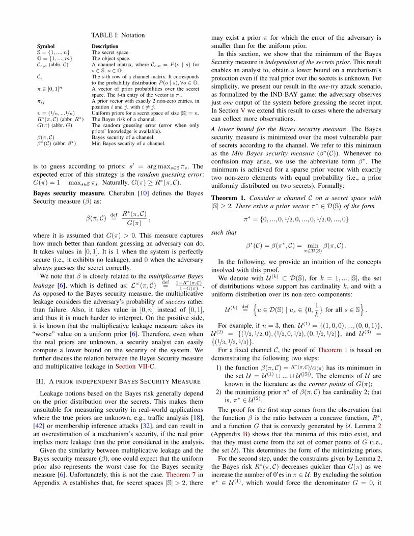
TABLE I: Notation

Symbol DescriptionS = {1, ..., n} The secret space.O = {1, ...,m} The object space.Cs,o (abbr. C) A channel matrix, where Cs,o = P (o | s) for

s ∈ S, o ∈ O.Cs The s-th row of a channel matrix. It corresponds

to the probability distribution P (o | s),∀o ∈ O.π ∈ [0, 1]n A vector of prior probabilities over the secret

space. The i-th entry of the vector is πi.πij A prior vector with exactly 2 non-zero entries, in

position i and j, with i 6= j.υ = (1/n, ...1/n) Uniform priors for a secret space of size |S| = n.R∗(π, C) (abbr. R∗) The Bayes risk of a channel.G(π) (abbr. G) The random guessing error (error when only

priors’ knowledge is available).β(π, C) Bayes security of a channel.β∗(C) (abbr. β∗) Min Bayes security of a channel.

is to guess according to priors: s′ = arg maxs∈S πs. Theexpected error of this strategy is the random guessing error:G(π) = 1−maxs∈S πs. Naturally, G(π) ≥ R∗(π, C).

Bayes security measure. Cherubin [10] defines the BayesSecurity measure (β) as:

β(π, C) def=

R∗(π, C)G(π)

,

where it is assumed that G(π) > 0. This measure captureshow much better than random guessing an adversary can do.It takes values in [0, 1]. It is 1 when the system is perfectlysecure (i.e., it exhibits no leakage), and 0 when the adversaryalways guesses the secret correctly.

We note that β is closely related to the multiplicative Bayesleakage [6], which is defined as: L×(π, C) def

= 1−R∗(π,C)1−G(π) .

As opposed to the Bayes security measure, the multiplicativeleakage considers the adversary’s probability of success ratherthan failure. Also, it takes value in [0, n] instead of [0, 1],and thus it is much harder to interpret. On the positive side,it is known that the multiplicative leakage measure takes its“worse” value on a uniform prior [6]. Therefore, even whenthe real priors are unknown, a security analyst can easilycompute a lower bound on the security of the system. Wefurther discuss the relation between the Bayes Security measureand multiplicative leakage in Section VII-C.

III. A PRIOR-INDEPENDENT BAYES SECURITY MEASURE

Leakage notions based on the Bayes risk generally dependon the prior distribution over the secrets. This makes themunsuitable for measuring security in real-world applicationswhere the true priors are unknown, e.g., traffic analysis [18],[42] or membership inference attacks [32], and can result inan overestimation of a mechanism’s security, if the real priorimplies more leakage than the prior considered in the analysis.

Given the similarity between multiplicative leakage and theBayes security measure (β), one could expect that the uniformprior also represents the worst case for the Bayes securitymeasure [6]. Unfortunately, this is not the case. Theorem 7 inAppendix A establishes that, for secret spaces |S| > 2, there

may exist a prior π for which the error of the adversary issmaller than for the uniform prior.

In this section, we show that the minimum of the BayesSecurity measure is independent of the secrets prior. This resultenables an analyst to, obtain a lower bound on a mechanism’sprotection even if the real prior over the secrets is unknown. Forsimplicity, we present our result in the one-try attack scenario,as formalized by the IND-BAY game: the adversary observesjust one output of the system before guessing the secret input.In Section V we extend this result to cases where the adversarycan collect more observations.

A lower bound for the Bayes security measure. The Bayessecurity measure is minimized over the most vulnerable pairof secrets according to the channel. We refer to this minimumas the Min Bayes security measure (β∗(C)). Whenever noconfusion may arise, we use the abbreviate form β∗. Theminimum is achieved for a sparse prior vector with exactlytwo non-zero elements with equal probability (i.e., a prioruniformly distributed on two secrets). Formally:

Theorem 1. Consider a channel C on a secret space with|S| ≥ 2. There exists a prior vector π∗ ∈ D(S) of the form

π∗ = {0, ..., 0, 1/2, 0, ..., 0, 1/2, 0, ..., 0}

such that

β∗(C) = β(π∗, C) = minπ∈D(S)

β(π, C) .

In the following, we provide an intuition of the conceptsinvolved with this proof.

We denote with U (k) ⊂ D(S), for k = 1, ..., |S|, the setof distributions whose support has cardinality k, and with auniform distribution over its non-zero components:

U (k) def={u ∈ D(S) | us ∈ {0,

1

k} for all s ∈ S

}.

For example, if n = 3, then: U (1) = {(1, 0, 0), ..., (0, 0, 1)},U (2) = {(1/2, 1/2, 0), (1/2, 0, 1/2), (0, 1/2, 1/2)}, and U (3) ={(1/3, 1/3, 1/3)}.

For a fixed channel C, the proof of Theorem 1 is based ondemonstrating the following two steps:

1) the function β(π, C) = R∗(π,C)/G(π) has its minimum inthe set U = U (1) ∪ ... ∪ U (|S|). The elements of U areknown in the literature as the corner points of G(π);

2) the minimizing prior π∗ of β(π, C) has cardinality 2; thatis, π∗ ∈ U (2).

The proof for the first step comes from the observation thatthe function β is the ratio between a concave function, R∗,and a function G that is convexly generated by U . Lemma 2(Appendix B) shows that the minima of this ratio exist, andthat they must come from the set of corner points of G (i.e.,the set U ). This determines the form of the minimizing priors.

For the second step, under the constraints given by Lemma 2,the Bayes risk R∗(π, C) decreases quicker than G(π) as weincrease the number of 0’es in π ∈ U . By excluding the solutionπ∗ ∈ U (1), which would force the denominator G = 0, it

follows that the minimizer of β(π, C), π∗, has exactly 2 non-zero elements; that is, π∗ ∈ U (2).Importance of Theorem 1. This theorem has two importantconsequences. First, it implies that an analyst can compute β∗ inO(n2), where n is the size of the secret space. This is a drasticreduction in complexity compared with exhaustive search,which requires O(n!) operations. In Section IV, we showthat the properties derived from Theorem 1 enable even moreefficient estimation of β∗, and that when domain knowledgeis available, it can be computed with a single measurement.

Second, it provides an intuitive interpretation for β∗. Letus consider the example in Figure 1. We see the posteriordistribution for five secret inputs obfuscated by a channelthat adds noise from a two-dimensional Laplacian distribution.Theorem 1 implies that the Min Bayes security measure,β∗, represents how far away are the posterior distributionsof the most distinguishable secrets (shown in red). This isin contrast with differential privacy, which ensures that thedistance between the worst-case outputs (those that providethe best chance to distinguish the worst-case two secrets) issmall enough. Enforcing worst-case protection results in verypessimistic security estimation, and in many cases imposes asignificant performance penalty. Conversely, good protection interm of Min Bayes security can be obtained with little impacton utility. We show that β∗ is a reasonable relaxation of LocalDifferential Privacy in Section VII, and demonstrate it providesa good security vs. utility trade-off in Section VI.

Fig. 1: Posterior probability distribution for 5 secrets obfuscatedusing a two-dimensional Laplacian. The Min Bayes securitymeasure, β∗, captures the distance between the posterior ofthe most distinguishable secrets (shown in red).

IV. EFFICIENT COMPUTATION OF β∗

Theorem 1 shows that to quantify Min Bayes security, theminimizer of Bayes security, we just need to estimate β for allpairs of secrets, that is in O(n2) measurements. A measurementfor a pair of secrets is obtained by estimating the Bayes risk ofthe mechanism for those two secrets; we can do this analytically,if we have white-box knowledge of the mechanism, or ina black-box manner [11]. In either case, if the mechanismis complex enough (e.g., large input or output space), eachmeasurement may need a non-negligible computational time,from seconds to tens of minutes.

In this section, we investigate techniques for improving thesearch time. Since the bottleneck is the time it takes to measureβ(π, C) for one prior π, we seek to reduce the number of suchmeasurements. We first assume white-box knowledge of thesystem (subsections IV-A-IV-C), and then study the black-boxcase (subsection IV-D).Initial observations. Denote by πab be the sparse prior vector(0, ..., 0, 1/2, 0, ..., 0, 1/2, 0, ..., 0) such that the two non-zeroelements of value 1/2 are in positions a and b, and a 6= b.Given a channel C, from the definition of β we get that

β(πab, C) = 2−∑o

maxs∈{a,b}

Cs,o .

The crucial observation (shown in the proof of Theorem 2) isthat the above quantity is equal to one minus the total variationdistance tv(Ca, Cb) between the rows Ca and Cb of the channel,which are probability distributions. The total variation distanceof two discrete distribution is 1/2 of their L1 distance (seen asvectors); hence we have that:

β(πab, C) = 1− tv(Ca, Cb) = 1− 1

2‖Ca − Cb‖1 .

Then, from Theorem 1, we get that minimizing β isequivalent to finding the rows of the channel that are maximallydistant with respect to L1.

Theorem 2. For any channel C, it holds that

β∗(C) = 1− 1

2maxa,b∈S

‖Ca − Cb‖1 .

This is the well-known diameter problem (for L1): giventhe set of vectors CS, find the two that are maximally distant(i.e., find the diameter of the set).

A. Computing β∗ with domain knowledge

In practical applications, domain knowledge may enable apriori identification of the two leakiest secrets. For example,the smallest and largest webpages users can visit in websitefingerprinting; and the smallest and largest exponents in timingside channels against exponentiation algorithms. In other casesall the secrets are equally vulnerable, and hence any two secretsare the most vulnerable. For instance, when the mechanismoperates in such a way that all secrets enjoy the same protection(e.g., the Randomized Response mechanism, Section VI).

Under these circumstances the secret space becomes binary(i.e., |S| = 2) and β∗ becomes the Bayes security measureover the uniform prior υ = (1/2, 1/2). More generally, if onedoes not know the exact minimizing secrets, but knows thatthey belong to a set S′ ⊂ S, then to determine β∗ it sufficesmeasuring β for all s1, s2 ∈ S′.

B. Computing β∗ in linear time n

The geometric characterization given by Theorem 2 impliesthat obtaining β∗ requires to compute the diameter of a set ofn = |S| vectors of dimension m = |O|. The direct approachis to compute the distance between every pair of vectors, i.e.,perform O(n2m) operations. This quadratic dependence on ncan be prohibitive when the number of secrets grows.

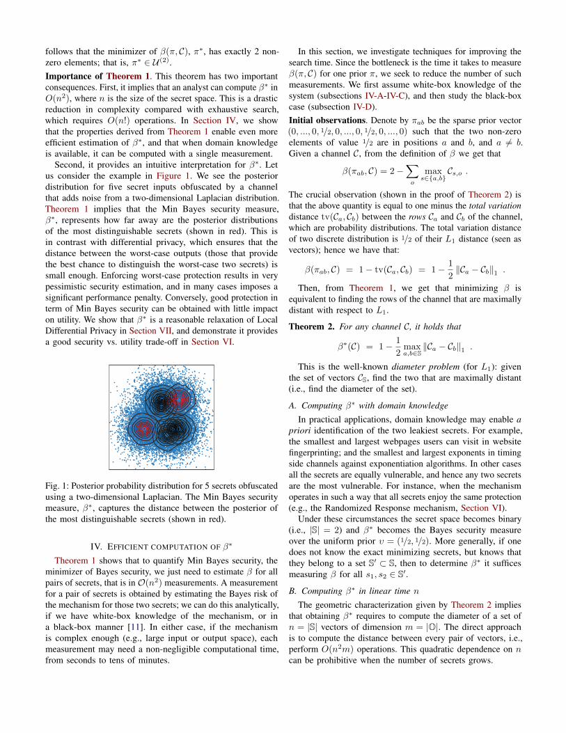
Fig. 2: β∗ and bounds for Rand. Response. Left: |S| = |O| = 10while varying ε. Right: ε = 0.5 while varying |S| = |O|.

We first show that, by using a well-known isometricembedding of Lm1 into L2m

∞ , β∗ can be computed in O(n2m)time. Concretely, each x ∈ Rm is translated into a vectorφ(x) ∈ R2m , which has one component for every bitstringb of length m, such that φ(x)b =

∑mi=1 xi(−1)bi . Note that

the equivalence ‖φ(x) − φ(x′)‖∞ = ‖x − x′‖1 holds for allx, x′ ∈ Rm. The L∞ diameter problem can be solved in lineartime: we only need to find the maximum and minimum valueof each component.

This computation is linear on |S|, but still exponential in|O|. It outperforms the direct approach when the number ofobservations remains small, though the problem becomes harderas the number of observations grows. When m = Θ(n) thereis no sub-quadratic algorithm for the Lp-diameter problem forany p ≥ 0 [13] . This suggests that there may not be anysub-quadratic time for computing β∗ either.

C. An efficient approximation of β∗

We now present an estimation of β∗ that can be obtained inO(nm) time. One selects an arbitrary distribution q ∈ D(O)and computes the maximal distance d between any channelrow and q. The diameter of CS is at most 2d, giving a lowerbound on β∗. Furthermore, if q lies within the convex hull ofCS (denoted by ch(CS)), then the diameter is at least d, givingalso an upper bound:

Proposition 1. Let C be a channel, q ∈ D(O), and d =maxs∈S ‖Cs − q‖1. Then 1 − d ≤ β∗(C) . Moreover, if q ∈ch(CS) then β∗(C) ≤ 1− d/2 .

Good choices for q are distributions that are likely to lie“in-between” the two maximally distant rows, for instance thecentroid of CS (mean of all rows).

Several advanced approximation algorithms exist for theL2 diameter problem [23]; these could be employed usingsome embedding of L1 into L2. The trivial embedding hasdistortion

√m (since ‖x‖2 ≤ ‖x‖1 ≤

√m‖x‖2), hence the

approximation factor may be too loose as |O| grows. Lowdistortion embeddings of L1 into L2 exist [4], but it is unclearwhether they can be effectively applied to the diameter problem.

In Figure 2 we show β∗ and various lower bounds for theRandomized Response mechanism (RR) (see Section VI-B).Two of the bounds are obtained via Proposition 1, by setting

q to be the mean row (the uniform distribution for RR) andany row of C (all rows are equal for RR). The third bound isobtained via the L2-diameter by using the trivial embedding.The mean-row bound is the most accurate in this case.

D. Black-box estimation of β∗

The previous sections assume full knowledge of the channelC. In practice this assumption may fail: systems may be toocomplex to analyze, or their behavior may be unknown. In suchcases, we can estimate the Bayes risk, and therefore, β usingtools such as F-BLEAU for black-box estimation black-boxway (i.e., only observing the system’s inputs and outputs) [11].As with the white-box case, we need to reduce the number ofpriors π for which we estimate β(π,C).

Bounds. A first approach is to use the bounds given byProposition 1, which can be computed in a black-box setting.One can interact with the system to obtain observations for q.For instance observe: the mean row, by drawing observationsfrom the channel with secrets that are chosen uniformly atrandom; the any row of the channel, by drawing observation fora secret chosen arbitrarily; or a row with arbitrary distribution,e.g., by sampling q uniformly at random from the set O.

Building on R∗ black-box estimators [11]. As observed inSection IV-A if domain constraints enable to identify the pair ofleakiest secrets, we can limit the search to those; this principlealso applies to the black-box setting. If this is not the case, thenone can try to reduce the search space. A promising approach isto exploit the triangle inequality on the total variation distanceto discard some solutions before computing them. For example,given the Bayes security for the priors πac and πbc:

β(πac, C) + β(πbc, C)− 1 ≤ β(πab, C)≤ 1− |β(πac, C)− β(πbc,C)| .

Thus, if β(πab, C) is larger than some already-known β(πij , C)there is no need to compute it. Conversely, if it is upperbounded by a small quantity, we can compute it earlier aimingat discarding other combinations.

V. THE BAYES SECURITY MEASURE UNDER COMPOSITION

In the previous sections we considered the case wherethe adversary observes one output from one channel. Thisscenario facilitates the derivation of proofs, but it does notcover many scenarios arising in reality. It is common thatthe adversary observes more than one channel at a time,e.g., observing obfuscated locations at different layers [38]or combining side channels [34]. They can observe the outputof two sequential channels, e.g., observing users privacy-preserving interactions with a database through and anonymouscommunication channel [36]; or they can observe more thanone output from one channel, e.g., gathering several sidechannel measurements from a cryptographic hardware [26],or observing more than one visit to a website through ananonymous communication channel [24], [39].

A. Parallel composition

We first consider the adversary has access to the outputsof two channels that have as input the same secret [34],[38] or where an adversary observes multiple channel outputsbelonging to the same secret [24], [26], [39].

Given two channels, C1 : S → O1 and C2 : S → O2, theirparallel composition is the channel C1||C2 : S → O1 × O2,defined by (C1||C2)s,(o1,o2) = C1s,o1 · C

2s,o2 .

Theorem 3. For all channels C1, C2 it holds that

β∗(C1||C2) ≥ β∗(C1) · β∗(C2) .

In layman terms, the composition of two channels that arerespectively β∗1 -secure and β∗2 -secure leads to a β∗1β

∗2 -secure

channel. The security of this new channel is not necessarilyminimized by the secrets that minimize the composing channelsC1, C2, not even when the channel is composed with itself:

Proposition 2. Let C be a channel for which β is minimizedfor secrets (s1, s2). Then the composition channel C′ := C||Cis not necessarily minimized by secrets (s1, s2).

Proof. A counterexample follows.

C =

0.9 0.1 0.00.8 0.2 0.00.5 0.5 0.00.5 0.1 0.4

β∗(C) = 0.6 is obtained for secrets (s1, s3); β∗(C||C) = 0.36is achieved for secrets (s2, s4).

B. Chaining mechanisms

Another typical configuration to strengthen the security ofthe system, is to put in place a cascade of security mechanisms(in-depth security). More formally, consider two channels C1 :S1 7→ S2 and C2 : S2 7→ O. Their cascade composition isthe channel C1C2 in which the secret is input in C1 and thischannel’s output is post-processed by C2.

It is well understood that post-processing cannot decreasethe security of a mechanism. Therefore, C1C2 should be atleast as secure ask C1. Indeed, based on the concavity of R∗,it is easy to show that R∗(π, C1C2) ≥ R∗(π, C1) for any priorπ. Consequently, β(π, C1C2) ≥ β(π, C1).

Understanding the effect of C1 on C2 is less straightforward.The composition C1C2 can be seen as the pre-processing of C2,which is not necessarily a safe operation. Note that C2 receivesas input the output of C1, which is not necessarily the same asS1. Hence, the prior π on the input secret in S1 is meaninglessfor C2. Remarkably, as β∗ does not depend on the prior, itallows to compare C1C2 and C2 despite the different inputspaces. From Theorem 2 we know that β∗(C1C2) is given bythe maximum `1 distance between the rows of C1C2. The keyobservation is that the rows of C1C2 are convex combinationsof the rows of C2; but convex combinations cannot increasedistances, which brings us to the following result.

Theorem 4. For all channels C1, C2 it holds that

β∗(C1C2) ≥ max{β∗(C1), β∗(C2)} .

This means that neither pre-processing nor post-processingdecreases the Min Bayes security provided by a mechanism.

VI. MIN BAYES SECURITY EXAMPLE APPLICATIONS

We evaluate Min Bayes security over three privacy and secu-rity applications. We compare it with Differential Privacy [17]and Local Differential Privacy [15] (see Section VII) on twoprivacy applications: quantifying machine learning models’vulnerability to membership attacks [32], and quantifyingthe obfuscation strength of Randomized Response (RR) [19],[41], respectively. We then use β∗ to measure vulnerabilityin a security-oriented application: quantifying the leakage ofPseudorandom Number Generators (PRNGs); in this use case,we also demonstrate that β∗ can be computed with only onemeasurement when we have domain knowledge.

A. Membership Inference attacks

As machine learning as a service becomes pervasive, thethreat of Membership inference attacks (MIA) grows inimportance. In this section we use this use case to comparethe Min Bayes security measure with Differential Privacy.

Membership Inference. In MIA an adversary aims to predictwhether an example was a member of the model’s trainingset. Consider a machine learning classifier f(x) : Rd 7→ [0, 1]p

trained on a private dataset of records belonging to p classes.For each input x, this classifier outputs a confidence vector in[0, 1]p expressing the confidence that x belongs to each class.The adversary observes this confidence vector, and guesseswhether x was a member of the classifier’s training set.

This attack can be seen as an instance of the IND-BAY game(see Section II) in which the secret input is the membershipof a record, i.e., s ∈ S = {in, out}; and the channel’s outputis the confidence vector output by the model, o ∈ O = [0, 1]p.

Differentially private (DP) machine learning. Many workspropose methods to train machine learning models such thatthe output is differentially private [1], [9], [31]. Such trainingimplies that the model is not be strongly affected by anyindividual training point, and thus the model’s outputs shouldnot vary depending on whether a specific record is present intraining or not. In other words, DP should be a good defenseagainst MIA.

We use the ε-differentially private logistic regression clas-sifier included in Diffprivlib [22], which is based onthe work by Chaudhuri et al. [9]. While tighter techniqueshave been proposed afterwards [1], [31], there are no availableimplementations that work properly on our small datasets. Inany case, we argue that for the purpose of illustrating thedifferences between the security measures under study.

Datasets. We consider two datasets. First, the MNISTdataset [28], widely used in the machine learning community.It comprises 60,000 images of handwritten digits. Each imageis a 28×28 grayscale pixel matrix. The classification task is to,

given an image, predict the digit. Second, the Texas HospitalDischarge (THD) dataset [35], which was used for evaluatingMIA by Shokri et al. [32]. It includes 67,330 records aboutpatients stays in several hospitals. The classification task is topredict the main procedure for each patient, based on the causeof the injury, the diagnosis, and generic information about thepatient (e.g., age, race, gender).

These datasets enable us to test Bayes security on a well-trained model (MNIST) and a model that does not offer goodperformance (THD). This is very relevant, as previous workshowed that the badness of a model is positively correlatedwith its vulnerability to MIA [32], [44].

Methodology. First, we split the datasets into training andvalidation sets. To emphasize the vulnerability of the modelsto MIA [44], as Shokri et al. [32], we train the models on alimited number of examples and do not optimize the learninghyperparameters to avoid overfitting. We use 15K trainingexamples for MNIST and 10K for THD, which leaves 45K and57,330 examples for validation, respectively. We report resultsfor one partition, but others provide very similar values.

Second, we train a logistic regression without DP. Unex-pectedly, we find that training on THD results in overfitting(Training accuracy=0.93 and Validation accuracy 0.58) and thatMNIST provides good performance (Training accuracy=0.95and Validation accuracy 0.88). This suggests that the lattermodel will be less vulnerable to MIA regardless of the noiseintroduced by the DP mechanism.

Third, we train several ε-DP logistic regression models usingDiffprivlib. For each model we evaluate utility as itsaccuracy on the validation set; and the Min Bayes securityusing the fbleau library [11]. We feed fbleau the samenumber of examples in and out of the training set, choosing theout examples at random. As recommended by the authors, weestimate the Bayes risk averaging 5 runs for all the availableestimators, and taking the smallest estimator as β∗.

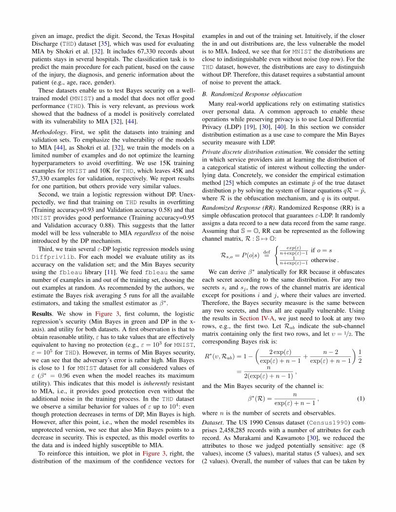
Results. We show in Figure 3, first column, the logisticregression’s security (Min Bayes in green and DP in the x-axis). and utility for both datasets. A first observation is that toobtain reasonable utility, ε has to take values that are effectivelyequivalent to having no protection (e.g., ε = 103 for MNIST,ε = 105 for THD). However, in terms of Min Bayes security,we can see that the adversary’s error is rather high. Min Bayesis close to 1 for MNIST dataset for all considered values ofε (β∗ = 0.96 even when the model reaches its maximumutility). This indicates that this model is inherently resistantto MIA, i.e., it provides good protection even without theadditional noise in the training process. In the THD datasetwe observe a similar behavior for values of ε up to 104: eventhough protection decreases in terms of DP, Min Bayes is high.However, after this point, i.e., when the model resembles itsunprotected version, we see that also Min Bayes points to adecrease in security. This is expected, as this model overfits tothe data and is indeed highly susceptible to MIA.

To reinforce this intuition, we plot in Figure 3, right, thedistribution of the maximum of the confidence vectors for

examples in and out of the training set. Intuitively, if the closerthe in and out distributions are, the less vulnerable the modelis to MIA. Indeed, we see that for MNIST the distributions areclose to indistinguishable even without noise (top row). For theTHD dataset, however, the distributions are easy to distinguishwithout DP. Therefore, this dataset requires a substantial amountof noise to prevent the attack.

B. Randomized Response obfuscation

Many real-world applications rely on estimating statisticsover personal data. A common approach to enable theseoperations while preserving privacy is to use Local DifferentialPrivacy (LDP) [19], [30], [40]. In this section we considerdistribution estimation as a use case to compare the Min Bayessecurity measure with LDP.Private discrete distribution estimation. We consider the settingin which service providers aim at learning the distribution ofa categorical statistic of interest without collecting the under-lying data. Concretely, we consider the empirical estimationmethod [25] which computes an estimate p of the true datasetdistribution p by solving the system of linear equations qR = p,where R is the obfuscation mechanism, and q is its output.Randomized Response (RR). Randomized Response (RR) is asimple obfuscation protocol that guarantees ε-LDP. It randomlyassigns a data record to a new data record from the same range.Assuming that S = O, RR can be represented as the followingchannel matrix, R : S 7→ O:

Rs,o = P (o|s) def=

{exp(ε)

n+exp(ε)−1 if o = s1

n+exp(ε)−1 otherwise .

We can derive β∗ analytically for RR because it obfuscateseach secret according to the same distribution. For any twosecrets si and sj , the rows of the channel matrix are identicalexcept for positions i and j, where their values are inverted.Therefore, the Bayes security measure is the same betweenany two secrets, and thus all are equally vulnerable. Usingthe results in Section IV-A, we just need to look at any tworows, e.g., the first two. Let Rab indicate the sub-channelmatrix containing only the first two rows, and let υ = 1/2. Thecorresponding Bayes risk is:

R∗(υ,Rab) = 1−(

2 exp(ε)

exp(ε) + n− 1+

n− 2

exp(ε) + n− 1

)1

2

=n

2(exp(ε) + n− 1),

and the Min Bayes security of the channel is:

β∗(R) =n

exp(ε) + n− 1, (1)

where n is the number of secrets and observables.Dataset. The US 1990 Census dataset (Census1990) com-prises 2,458,285 records with a number of attributes for eachrecord. As Murakami and Kawamoto [30], we reduced theattributes to those we judged potentially sensitive: age (8values), income (5 values), marital status (5 values), and sex(2 values). Overall, the number of values that can be taken by

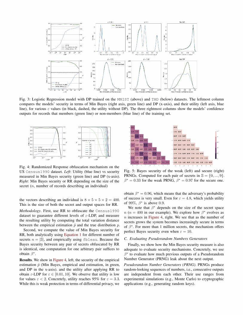
Fig. 3: Logistic Regression model with DP trained on the MNIST (above) and THD (below) datasets. The leftmost columncompares the models’ security in terms of Min Bayes (right axis, green line) and DP (x-axis), and their utility (left axis, blueline), for various ε values (in black, dashed, the utility without DP). The three rightmost columns show the models’ confidenceoutputs for records that members (green line) or non-members (blue line) of the training set.

Fig. 4: Randomized Response obfuscation mechanism on theUS Census1990 dataset. Left: Utility (blue line) vs securitymeasured in Min Bayes security (green line) and DP (x-axis).Right: Min Bayes security or RR depending on the size of thesecret (n, number of records describing an individual)

the vectors describing an individual is 8 × 5 × 5 × 2 = 400.This is the size of both the secret and output spaces for RR.

Methodology. First, use RR to obfuscate the Census1990dataset to guarantee different levels of ε-LDP, and measurethe resulting utility by computing the total variation distancebetween the empirical estimation p and the true distribution p.

Second, we compute the value of Min Bayes security forRR, both analytically using Equation 1 for different number ofsecrets n = |S|, and empirically using fbleau. Because theBayes security between any pair of secrets obfuscated by RRis identical, one computation for one arbitrary pair suffices toobtain β∗.

Results. We show in Figure 4, left, the security of the empiricalestimation p (Min Bayes, empirical and estimation, in green,and DP in the x-axis). and the utility after applying RR toobtain ε-LDP for ε ∈ [0.01, 10]. We observe that utility is lowfor values ε < 2. Concretely, utility reaches 95% for ε = 3.3.While this is weak protection in terms of differential privacy, we

Fig. 5: Bayes security of the weak (left) and secure (right)PRNGs. Computed for each pair of secrets in S = {0, ..., 9}.β∗ = 0.33 for the weak PRNG, β∗ = 0.97 for the secure one.

obtain β∗ = 0.96, which means that the adversary’s probabilityof success is very small. Even for ε = 4.8, which yields utilityof 99%, β∗ is above 0.9.

We note that β∗ depends on the size of the secret spacen (n = 400 in our example). We explore how β∗ evolves asn increases in Figure 4, right. We see that as the number ofsecrets grows the system becomes increasingly secure in termsof β∗. For more than 1 million secrets, the mechanism offersperfect Bayes security even when ε = 10.

C. Evaluating Pseudorandom Numbers Generators

Finally, we show how the Min Bayes security measure is alsoadequate to evaluate security mechanisms. Concretely, we useβ∗ to evaluate how much previous outputs of a PseudorandomNumber Generator (PRNG) leak about the next output.Pseudorandom Number Generators (PRNG). PRNGs producerandom-looking sequences of numbers, i.e., consecutive outputsare independent from each other. Their use ranges fromexperimental simulations (e.g., Monte Carlo) to cryptographicapplications (e.g., generating random keys).

The security of a PRNG can be expressed in terms ofthe IND-BAY game. The current output is the adversary’sobservation o, and the adversary aims at predicting the nextoutput: the secret s.Dataset. We consider two PRNG implementations containedin the Java API that output pseudorandom integers in [0, 9].A weak PRNG, java.util.Random whose use is highlydiscouraged for cryptographic purposes; and a secure PRNG,java.security.SecureRandom, that is is cryptograph-ically secure, i.e., informally speaking, its output is unpre-dictable given previous outputs.

We use two datasets [37] generated by Chotia et al. with500,000 pairs of consecutive outputs from the two PRNGs. [12].Methodology. For each pair of secrets (the second element ofthe pair), we split their observations (the first element of thepair) into training and test set. We use F-BLEAU to estimateeach pair’s Bayes risk. We take as Min Bayes security theminimum of these estimates.Results. We show the the pairwise Min Bayes security for bothPRNGs in Figure 5. This representation shows how Min Bayesenables to distinguish weak and secure implementations. In theweak one, it enables to identify the most vulnerable secrets:the pair (3,8) with β∗ = 0.33. For the secure PRNG we seethat there are no vulnerable secrets: all pairs yield β > 0.97.

VII. RELATION WITH OTHER NOTIONS

In the previous sections we presented β∗, discussed itproperties and showed how to compute it in an efficient manner.In this section, we compare it with three well-known securitynotions: Differential privacy, as the paradigmatic worst-casemetric; cryptographic advantage, the strictest average measurein the security community; and multiplicative leakage, a prior-agnostic average information leakage measure.

A. Cryptographic advantage

In cryptography, the advantage Adv of an adversary A isdefined assuming that there are two secrets (|S| = 2) withuniform prior in input to a channel C. Formally (e.g. [43]):

Adv(C,A)def= 2|RA(υ, C)− 1/2| .

The factor 2 serves to scale Adv within the interval [0, 1].Denoting by Adv(C) the advantage of the optimal (Bayes)

adversary and considering uniform prior π = υ, we derive:

β(υ, C) = 1− 2|R∗(υ, C)−G(υ)| = 1− Adv(C). (2)

In other words, the Bayes security measure can be seen as ageneralization of 1 − Adv for which the secret space S maycontain more than two secrets and priors are not necessarilyuniform. A difference is that β is defined for the optimaladversary, while Adv is a generic notion, which can be definedwith respect to other (weaker) adversaries.Min Bayes as IND-CPA security. In Section II we introducedthe IND-BAY game to formalize the adversarial setting capturedby the Bayes security measure. When considering this game inthe light of our main result in Section III, the IND-BAY game

IND-MINBAYAC1 : A ← C, π2 : A selects s1, s2 ∈ S

3 : sπ1,2← {s1, s2}

4 : oP (o|s)← O

5 : s′ ← A(o)6 : return s = s′

IND-LDPAC1 : A ← C, π2 : A selects s1, s2 ∈ S3 : A selects o ∈ O

4 : sP (s|o)← {s1, s2}

5 : s′ ← A(o)6 : return s = s′

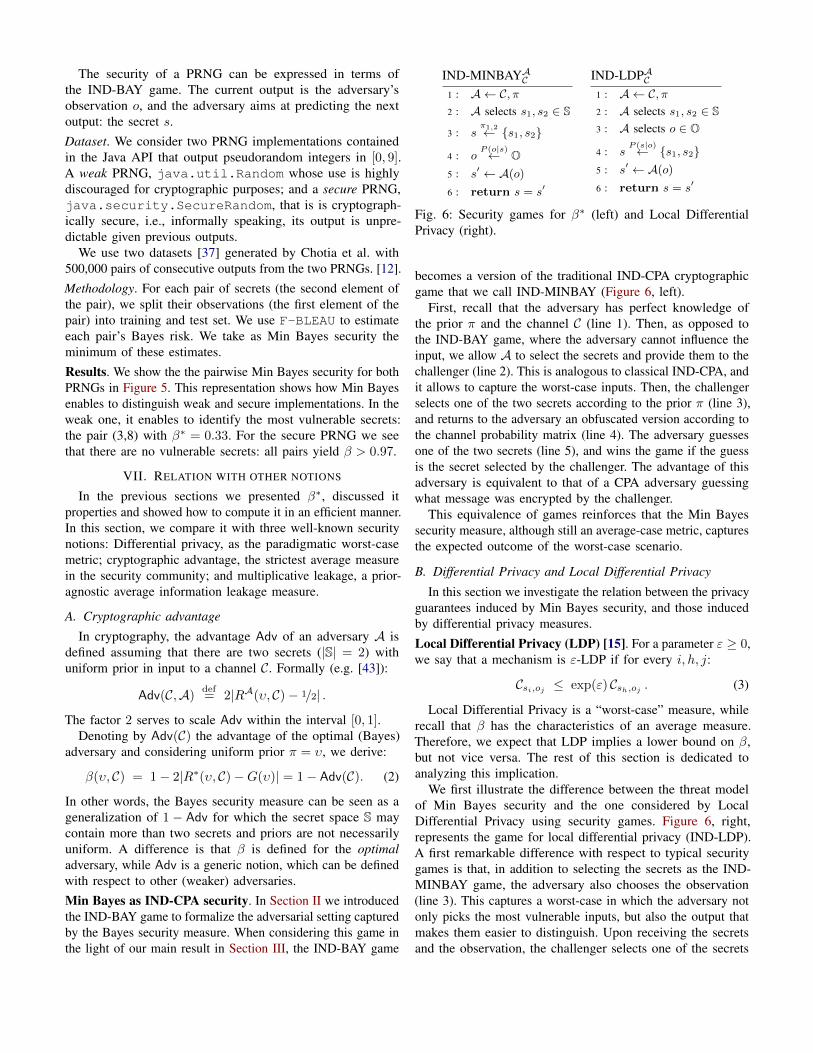
Fig. 6: Security games for β∗ (left) and Local DifferentialPrivacy (right).

becomes a version of the traditional IND-CPA cryptographicgame that we call IND-MINBAY (Figure 6, left).

First, recall that the adversary has perfect knowledge ofthe prior π and the channel C (line 1). Then, as opposed tothe IND-BAY game, where the adversary cannot influence theinput, we allow A to select the secrets and provide them to thechallenger (line 2). This is analogous to classical IND-CPA, andit allows to capture the worst-case inputs. Then, the challengerselects one of the two secrets according to the prior π (line 3),and returns to the adversary an obfuscated version according tothe channel probability matrix (line 4). The adversary guessesone of the two secrets (line 5), and wins the game if the guessis the secret selected by the challenger. The advantage of thisadversary is equivalent to that of a CPA adversary guessingwhat message was encrypted by the challenger.

This equivalence of games reinforces that the Min Bayessecurity measure, although still an average-case metric, capturesthe expected outcome of the worst-case scenario.

B. Differential Privacy and Local Differential Privacy

In this section we investigate the relation between the privacyguarantees induced by Min Bayes security, and those inducedby differential privacy measures.

Local Differential Privacy (LDP) [15]. For a parameter ε ≥ 0,we say that a mechanism is ε-LDP if for every i, h, j:

Csi,oj ≤ exp(ε) Csh,oj . (3)

Local Differential Privacy is a “worst-case” measure, whilerecall that β has the characteristics of an average measure.Therefore, we expect that LDP implies a lower bound on β,but not vice versa. The rest of this section is dedicated toanalyzing this implication.

We first illustrate the difference between the threat modelof Min Bayes security and the one considered by LocalDifferential Privacy using security games. Figure 6, right,represents the game for local differential privacy (IND-LDP).A first remarkable difference with respect to typical securitygames is that, in addition to selecting the secrets as the IND-MINBAY game, the adversary also chooses the observation(line 3). This captures a worst-case in which the adversary notonly picks the most vulnerable inputs, but also the output thatmakes them easier to distinguish. Upon receiving the secretsand the observation, the challenger selects one of the secrets

k︷ ︸︸ ︷a · · · a

m− k︷ ︸︸ ︷b · · · b

b · · · b a · · · ac · · · c c · · · c...

. . ....

.... . .

...c · · · c c · · · c

d e

m− 2︷ ︸︸ ︷0 · · · 0

e d 0 · · · 01 0 0 · · · 0...

......

. . ....

1 0 0 · · · 0

Fig. 7: Two examples of n ×m matrices C∗ which achieveminimum β value β∗C∗ = 2

1+exp(ε) . In the first matrix: a =exp(ε)

k(1+exp(ε)) , b = 1(m−k)(1+exp(ε)) and c = 1

m . In the second

matrix: d = exp(ε)1+exp(ε) and e = 1

1+exp(ε) .

according to the probability that it caused the observation (line4). A second difference with respect to typical games, andIND-MINBAY, is that the challenger does not show the chosenvalue to the adversary. Otherwise, it would be a trivial win.The adversary guesses a secret (line 5), and wins if this isthe secret the challenger chose (line 6). Note that, becausethe adversary has a much greater freedom in their choices,their chances to win are considerably greater than than inIND-MINBAY or traditional games. Therefore, the LDP gamecaptures stronger guarantees than most cryptographic game,but it is much harder to map IND-LDP to a realistic scenario.LDP induces a lower bound on Bayes security. In general,if there are no restrictions on the channel matrix, the lowestpossible value for β is 0, achieved when the adversary is ableto identify completely (i.e., with probability 1) the value of thesecret from every observable. Assuming that |S| ≥ 2 and thatπ is not concentrated on one single secret,1 and that S containsat least two elements, β can only be zero if and only if thechannel contains at most one non-0 value for each column.

If the matrix is exp(ε)-LDP, however, then the ratio betweentwo values on the same column is at most exp(ε). Intuitively,under this restriction, β cannot be 0 anymore: the best casefor the adversary is when the ratio is as large as possible, i.e.,when it is exactly exp(ε). In particular, in a 2× 2 channel, weexpect that the minimum β is achieved by a matrix that hasthe values exp(ε)/1+exp(ε) on the diagonal, and 1/1+exp(ε) inthe other positions (or vice versa). The next theorem confirmsthis intuition, and extends it to the general case n ×m. Werecall that β∗ = minπ β(π, C).

Theorem 5.1) If C is ε-LDP, then for every π we have

β(π, C) ≥ 21+exp(ε) .

2) For every n,m ≥ 2 there exists a n×m ε-LDP channelC∗ such that β∗(C∗) = 2

1+exp(ε) . Examples of such C∗’sare illustrated in Figure 7.

The Bayes security does not induce a lower bound on LDP.Theorem 5 shows that ε-LDP induces a bound on the minimal

1If the probability mass of π is concentrated on one secret, thenG(π) = 0 and β(π, C) is undefined. However also R∗(π, C) = 0, andlimπ′,→π β(π

′, C) = 1.

Bayes security, and that we can actually express a strict boundthat depends only on ε. The other direction does not hold. Themain reason is that if there is a 0 in a column which containsalso a positive element, then ε-LDP cannot hold, independentlyfrom the value of β.

One may consider (ε, δ)-LDP instead. This is a variant ofLDP in which small violations to the formula (3) are tolerated.More precisely, a mechanism is (ε, δ)-LDP if for every i, h, j:

Csi,oj ≤ exp(ε) Csh,oj + δ . (4)

With (ε, δ)-LDP, a column may contain 0 and non-0 values,as long as the latter are smaller than δ. So, one may wonderwhether Bayes security might imply a bound on (ε, δ)-LDP.The answer however is still no, at least, not in general. Thereason is that the two secrets that determine the value of βmay not be the same secrets that determine the min value of(ε, δ). The following is a counterexample.

Example 2. Consider the following channel matrix C.1/4 0 1/2 1/40 1/4 1/4 1/23/8 0 1/8 1/2

Let

π12def= (1/2, 1/2, 0) π13

def= (1/2, 0, 1/2) π23

def= (0, 1/2, 1/2).

Then: β(π12, C) = 1/2, β(π13, C) = 5/8, β(π23, C) = 5/8 .Hence β∗ = β(π12, C). However, from the comparison of

the first and second row we derive (ε, δ) ≥ (0, 1/4), whilefrom the comparison of the second and third row we derive(ε, δ) ≥ (0, 3/8), and from the comparison of the first and thirdrow we derive (ε, δ) ≥ (ln 4, 0). Since (0, 3/8) ≥ (0, 1/4), weconclude that the value of β∗, that in this case is determinedby the first and second row, does not allow to derive any (ε, δ)-LDP guarantee (i.e, it does not allow to derive the minimalvalues of (ε, δ) for which (ε, δ)-LDP holds).

Differential privacy [17]. Differential privacy is similar toLDP, except that it involves the notion of adjacent databases.Two databases x, x′ are adjacent, denoted as x ∼ x′, if x isobtained from x′ by removing or adding one record.

The definition of ε-differential-privacy (ε-DP), in the discretecase, is as follows. A mechanism K is ε-DP if for every x, x′

such that x ∼ x′, and every y, we have

P (K(x) = y) ≤ exp(ε)P (K(x′) = y).

A relation between the Bayes security and DP follows froman analogous result in [2] for the multiplicative Bayes leakageL×(π,K), and the correspondence between the latter and theBayes security (cfr. Section VII-C), which is given by

β(π, C) =1− (maxs πs)L×(π, C)

1−maxs πs. (5)

The following result, proved in [2], states that ε-DP inducesa bound on the multiplicative Bayes leakage, where the set ofsecrets are all the possible databases. The theorem is given forthe bounded DP case, where we assume that the number of

records present in the database is at most a certain number n,and that the set of values for the records includes a specialvalue ⊥ representing the absence of the record. The adjacencyrelation is modified accordingly: x ∼ x′ means that x and x′

differ for the value of exactly one record. We also assume thatthe cardinality v of the set of values is finite. Hence also thenumber of secrets (i.e., the possible databases) is finite.

Theorem 6 (From [2], Theorem 15). If K is ε-DP, then, forevery π, L×(π, C) is bounded from above as

L×(π, C) ≤(

v exp(ε)

v − 1 + exp(ε)

)n.

and this bound is tight when π is uniform.

From Theorem 6 and Equation 5 we immediately obtain abound also for the Bayes security:

Corollary 1. If K is ε-DP, then, for every π, β(π, C) is boundedfrom below as

β(π, C) ≥1− (maxs πs)

(v exp(ε)

v−1+exp(ε)

)n1−maxs πs

.

and this bound is tight when π is the uniform distribution υwhich assigns 1/vn to every database, in which case it case itcan be rewritten as

β(π, C) ≥vn −

(v exp(ε)

v−1+exp(ε)

)nvn − 1

.

In [2] it is shown that the reverse of Theorem 6 does nothold, and as a consequence the reverse of Corollary 1 doesnot hold either. The reason is analogous to the case of LDP: a0 in a position of a non-0-column implies that the mechanismcannot be DP, independently from the value of β.

In Corollary 1 the secrets are the whole databases. Often,however, in DP we assume that the attacker is not interestedat discovering the whole database, but only whether a certainrecords belongs to the database or not. We can model thiscase by isolating a generic pair of adjacent databases x and x′,and then restricting the space of secrets to be just {x, x′}. Onthis space, the mechanism can be represented by a stochasticchannel C{x,x′} that has only the two inputs x and x′, and asoutputs the (obfuscated) answers to the query. It is immediate tosee that K is ε-DP iff C{x,x′} is ε-LDP for any pair of adjacentdatabases x and x′. Hence, the results presented in previoussection concerning the relation between Bayes security andLDP hold also for DP. In particular, the following corollary isan immediate consequence of Theorem 5.

Corollary 2. If K is ε-DP, then for every pair of adjacentdatabases x and x′ and every π we have

β(π, C{x,x′}) ≥ 2

1 + exp(ε).

and this bound is strict.

A similar investigation was done by Yeom et al. [43]. Theystudied the privacy of C{x,x′} in terms of the advantage, defined

in the context of membership inference attacks (MIA); wediscuss and evaluate these attacks in Section VI-A. The authorsestablished that, if a mechanism is ε-DP, then the followinglower bound for holds for Adv(C{x,x′}), for any adjacentdatabases x and x′:

Adv(C{x,x′}) ≤ exp(ε)− 1 (6)

By using the relation between the advantage and the Bayessecurity measure (Equation 2), we derive the following bound:

β(υ, C{x,x′}) ≥ 2− exp(ε) . (7)

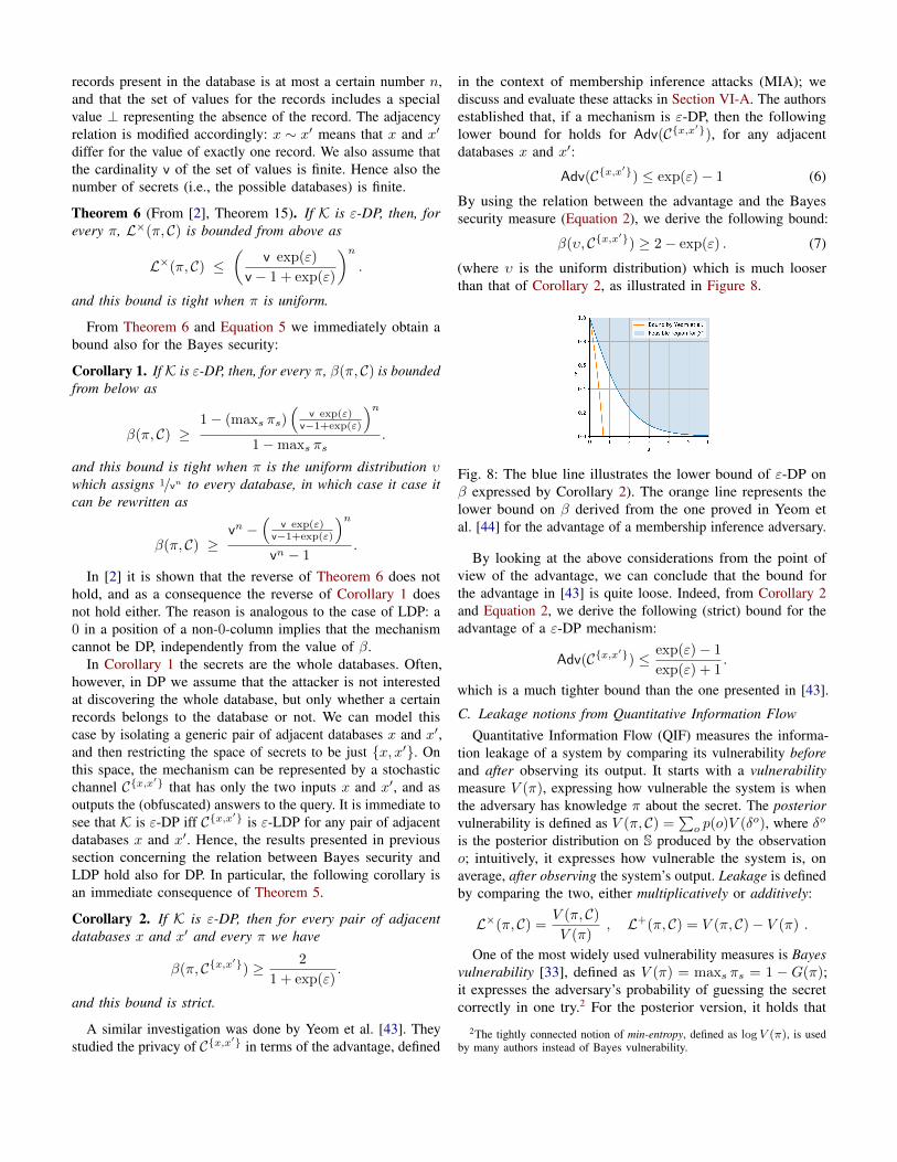
(where υ is the uniform distribution) which is much looserthan that of Corollary 2, as illustrated in Figure 8.

Fig. 8: The blue line illustrates the lower bound of ε-DP onβ expressed by Corollary 2). The orange line represents thelower bound on β derived from the one proved in Yeom etal. [44] for the advantage of a membership inference adversary.

By looking at the above considerations from the point ofview of the advantage, we can conclude that the bound forthe advantage in [43] is quite loose. Indeed, from Corollary 2and Equation 2, we derive the following (strict) bound for theadvantage of a ε-DP mechanism:

Adv(C{x,x′}) ≤ exp(ε)− 1

exp(ε) + 1.

which is a much tighter bound than the one presented in [43].

C. Leakage notions from Quantitative Information FlowQuantitative Information Flow (QIF) measures the informa-

tion leakage of a system by comparing its vulnerability beforeand after observing its output. It starts with a vulnerabilitymeasure V (π), expressing how vulnerable the system is whenthe adversary has knowledge π about the secret. The posteriorvulnerability is defined as V (π, C) =

∑o p(o)V (δo), where δo

is the posterior distribution on S produced by the observationo; intuitively, it expresses how vulnerable the system is, onaverage, after observing the system’s output. Leakage is definedby comparing the two, either multiplicatively or additively:

L×(π, C) =V (π, C)V (π)

, L+(π, C) = V (π, C)− V (π) .

One of the most widely used vulnerability measures is Bayesvulnerability [33], defined as V (π) = maxs πs = 1 − G(π);it expresses the adversary’s probability of guessing the secretcorrectly in one try.2 For the posterior version, it holds that

2The tightly connected notion of min-entropy, defined as log V (π), is usedby many authors instead of Bayes vulnerability.

V (π, C) = 1 − R∗(π, C). Bayes security follows the samecore idea: G(π) can be thought of as a prior version of R∗:indeed, it holds that R∗(π, C) =

∑o p(o)G(δo) where δo are

the posteriors of the channel. Hence, β can be considered tobe a variant of multiplicative leakage, using Bayes risk insteadof Bayes vulnerability.

Since the two are closely related, one would expect to be ableto directly translate results about L×(π, C) to similar resultson β(π, C). This would be the case for additive leakage, sinceV (π, C)− V (π) = G(π)−R∗(π, C), but in the multiplicativecase, the “one minus” in both sides of the fraction completelychanges the behavior of the function.

Capacity vs β∗. One should first note that, while β takes lowervalues to indicate a worse level of security, L× takes highervalues. In both cases, a natural question is to find the prior πthat provides the worst level of security; in the case of leakage,its maximum value is known as channel capacity, denoted byML×(C) = maxπ L×(π, C).ML×(C) is given by the uniform prior [6]. MoreoverML×(C) =

∑o maxs Cs,o. Our main result (Theorem 1)

shows that Bayes security is minimized on a uniform priorπab over 2 secrets. Hence, despite the similarity betweenBayes vulnerability and Bayes risk, the corresponding leakageand security measures behave very differently. This differencemakes ML×(C) much easier to compute; it is linear on both|S| and |O|, while β∗ is quadratic on |S|.Channel composition. Despite their difference w.r.t. the priorthat realizes each notion, ML× and β∗ behave similarly wrtboth parallel and cascade composition of channels. In [20], itis shown that

ML×(C1||C2) ≤ ML×(C1) · ML×(C2) , and

ML×(C1C2) ≤ min{ML×(C1),ML×(C2)} .

The exact same bounds are given in Section V for β∗. Note,however, that the proofs for β∗ are completely different andcannot be directly obtained from those ofML×. This is due tothe fact that the prior realizing β∗ for the composed channel isunknown, and possibly different that the one realizing β∗ forC1 and C2. This makes the proofs arguably harder than thosefor ML×, which is always achieved on the uniform prior.

Bounds on vulnerability and risk. Given the similarities betweenL× and β, as well as their differences, a natural question iswhich is more adequate for a particular application. The answer,naturally, depends on what we are trying to achieve.

It should be noted that the goal of a security analyst is toquantify how much information is leaked by a mechanism inthe worst case. This is captured by both ML× and β∗ whichfocus on the prior that produces the highest leakage instead ofthe actual prior, which is unknown to the adversary.

The user, however, is mostly interested in the actual threatthat he is facing: how likely it is for the adversary to guesshis secret, given a particular prior π that captures the user’sbehavior. This corresponds to R∗(π, C). Bayes risk has a clearoperational interpretation for the user.

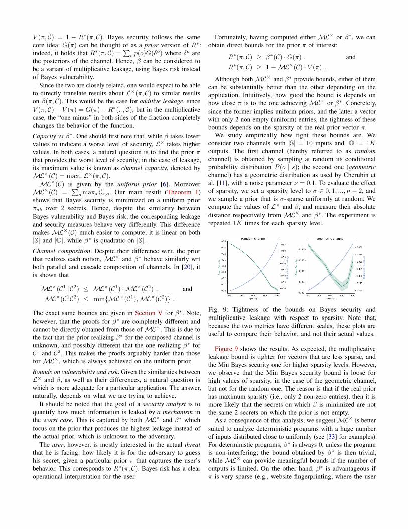
Fortunately, having computed either ML× or β∗, we canobtain direct bounds for the prior π of interest:

R∗(π, C) ≥ β∗(C) ·G(π) , and

R∗(π, C) ≥ 1−ML×(C) · V (π) .

Although both ML× and β∗ provide bounds, either of themcan be substantially better than the other depending on theapplication. Intuitively, how good the bound is depends onhow close π is to the one achieving ML× or β∗. Concretely,since the former implies uniform priors, and the latter a vectorwith only 2 non-empty (uniform) entries, the tightness of thesebounds depends on the sparsity of the real prior vector π.

We study empirically how tight these bounds are. Weconsider two channels with |S| = 10 inputs and |O| = 1Koutputs. The first channel (hereby referred to as randomchannel) is obtained by sampling at random its conditionalprobability distribution P (o | s); the second one (geometricchannel) has a geometric distribution as used by Cherubin etal. [11], with a noise parameter ν = 0.1. To evaluate the effectof sparsity, we set a sparsity level to σ ∈ 0, 1, ..., n− 2, andwe sample a prior that is σ-sparse uniformly at random. Wecompute the values of L× and β, and measure their absolutedistance respectively from ML× and β∗. The experiment isrepeated 1K times for each sparsity level.

Fig. 9: Tightness of the bounds on Bayes security andmultiplicative leakage with respect to sparsity. Note that,because the two metrics have different scales, these plots areuseful to compare their behavior, and not their actual values.

Figure 9 shows the results. As expected, the multiplicativeleakage bound is tighter for vectors that are less sparse, andthe Min Bayes security one for higher sparsity levels. However,we observe that the Min Bayes security bound is loose forhigh values of sparsity, in the case of the geometric channel,but not for the random one. The reason is that if the real priorhas maximum sparsity (i.e., only 2 non-zero entries), then it ismore likely that the secrets on which β is minimized are notthe same 2 secrets on which the prior is not empty.

As a consequence of this analysis, we suggestML× is bettersuited to analyze deterministic programs with a huge numberof inputs distributed close to uniformly (see [33] for examples).For deterministic programs, β∗ is always 0, unless the programis non-interfering; the bound obtained by β∗ is then trivial,while ML× can provide meaningful bounds if the number ofoutputs is limited. On the other hand, β∗ is advantageous ifπ is very sparse (e.g., website fingerprinting, where the user

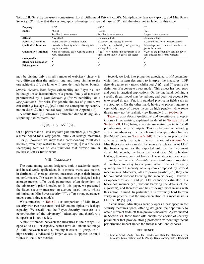
TABLE II: Security measures comparison: Local Differential Privacy (LDP), Multiplicative leakage capacity, and Min BayesSecurity (β∗). Note that the cryptographic advantage is a special case of β∗, and therefore not included in this table.

Property LDP ML× β∗

Range [0,∞) [1,∞) [0, 1]

Smaller is more secure Smaller is more secure Larger is more secureAttacks Any attack Concrete attack Concrete attackSecurity Guarantee Worst case for 2 leakiest secrets Expected risk among all secrets Expected risk for 2 leakiest secretsQualitative Intuition Bounds probability of ever distinguish-

ing two secretsBounds the probability of guessingamong all secrets

Advantage w.r.t. random baseline toguess the secret

Quantitative Intuition None for general case. Can be definedw.r.t. mechanism

ML× = k means the adversary is ktimes more likely to guess the secret

1/2β∗ is the probability that the adver-sary guesses the secret correctly

Composable 3 3 3

Black-box Estimation 7 3 3

Prior-agnostic 3 3 3

may be visiting only a small number of websites): since π isvery different than the uniform one, and more similar to theone achieving β∗, the latter will provide much better bounds.

Miracle theorem. Both Bayes vulnerability and Bayes risk canbe thought of as instantiations of a general family of measuresparametrized by a gain function g (for vulnerability) or aloss function ` (for risk). For generic choices of g and `, wecan define g-leakage L×g (π, C) and the corresponding securitynotion β`(π, C), in a natural way (detailed in Appendix F).

A result from [3], known as “miracle” due to its arguablysurprising nature, states that

L×g (π, C) ≤ ML×(C) ,

for all priors π and all non-negative gain functions g. This givesa direct bound for a very general family of leakage measures.

For β`, however, we know that a corresponding result doesnot hold, even if we restrict to the family of [0, 1] loss functions.Identifying families of loss functions that provide similarbounds is left as future work.

VIII. TAKEAWAYS

The trend among system designers, both in academic papersand in real-world applications, is to choose worst-case metricsin detriment of average-oriented measures despite their impacton performance. The reason is that mechanisms designed usingaverage metrics offer weak guarantees, often dependent onthe adversary’s prior knowledge. In this paper, we presentedthe Bayes security measure, an average-based metric whoseminimization, Min Bayes security (β∗), offers strong guaranteesunder certain threat models.

We summarize in Table II our comparison of Min Bayessecurity with two measures: local DP and multiplicative leakagecapacity. We recall that the Bayes Security measure is ageneralization of the adversary’s advantage and therefore acomparison is not needed.

A first difference between the measures is their range. Asopposed to LDP or capacity, which have an unbounded range,β∗ falls between 0 and 1, making it easier to grasp. In β∗

high security is indicated by larger values, as opposed to smallvalues in the other metrics.

Second, we look into properties associated to risk modeling,which help system designers to interpret the measures. LDPdefends against any attack, whilst bothML× and β∗ require thedefinition of a concrete threat model. This aspect has both prosand cons in practical applications. On the one hand, defining aspecific threat model may be tedious, and does not account forunexpected threats. Yet, it is standard practice in fields such ascryptography. On the other hand, having to protect against avery wide range of threats incurs on high penalty, while somethreats may not be realistic (see Example 1 in Section I).

Table II also details qualitative and quantitative interpre-tations of the metrics, explained in detail in Section III andSection VII. LDP, being a worst-case metric, protects for allpossible mechanism’s outputs. This can be seen as defendingagainst an adversary that can choose the outputs she observes(IND-LDP game in Section VII-B). However, in practice theadversary rarely ever gets to select the output (Section VI).Min Bayes security can also be seen as a relaxation of LDP:the former quantifies the expected risk for the two mostvulnerable secrets, the latter the worst case. Multiplicativeleakage, however, does not have a clear relation in these terms.

Finally, we consider desirable system evaluation properties.All metrics are easy to compose, which enables to easilyquantify overall security of a system composed by severalmechanisms. Moreover, all are prior-agnostic (i.e., they canbe computed without knowing the secrets’ prior). However,as opposed to ML× and β∗, LDP cannot be estimated in ablack-box manner (i.e., without knowing the details of thealgorithm), and therefore one has to design mechanisms withthis notion in mind. In particular, it is extremely hard to evenverify in practice that the implementation of a mechanism isLDP or DP [5], [14].

In conclusion, Min Bayes security opens a new space in thesecurity measures space, offering designers the opportunity toobtain different trade-off than previous measures. As we showedin Section VI, these trade-offs enable the choice of securityparameters that provide strong protection without significantperformance impact under the threat model one chooses.

REFERENCES

[1] Martin Abadi, Andy Chu, Ian Goodfellow, Brendan McMahan, IlyaMironov, Kunal Talwar, and Li Zhang. Deep learning with differential

privacy. In Proc. of CCS, 2016.[2] Mário S. Alvim, Miguel E. Andrés, Konstantinos Chatzikokolakis,

Pierpaolo Degano, and Catuscia Palamidessi. On the information leakageof differentially-private mechanisms. J. of Comp. Security, 23(4):427–469,2015.

[3] Mário S. Alvim, Konstantinos Chatzikokolakis, Catuscia Palamidessi,and Geoffrey Smith. Measuring information leakage using generalizedgain functions. In Proc. of CSF, pages 265–279. IEEE, 2012.

[4] Sanjeev Arora, James R. Lee, and Assaf Naor. Euclidean distortion andthe sparsest cut. In STOC, pages 553–562. ACM, 2005.

[5] Benjamin Bichsel, Timon Gehr, Dana Drachsler-Cohen, Petar Tsankov,and Martin T. Vechev. Dp-finder: Finding differential privacy violationsby sampling and optimization. In Proc. of CCS, 2018.

[6] Christelle Braun, Konstantinos Chatzikokolakis, and Catuscia Palamidessi.Quantitative notions of leakage for one-try attacks. ENTCS, 249:75–91,2009.

[7] Konstantinos Chatzikokolakis, Tom Chothia, and Apratim Guha. Statisti-cal measurement of information leakage. In Proc. of TACAS, 2010.

[8] Konstantinos Chatzikokolakis, Catuscia Palamidessi, and Prakash Panan-gaden. On the Bayes risk in information-hiding protocols. J. of Comp.Security, 16(5):531–571, 2008.

[9] Kamalika Chaudhuri, Claire Monteleoni, and Anand D Sarwate. Differ-entially private empirical risk minimization. JMLR, 12(Mar):1069–1109,2011.

[10] Giovanni Cherubin. Bayes, not naïve: Security bounds on websitefingerprinting defenses. Proceedings on Privacy Enhancing Technologies,4:215–231, 2017.

[11] Giovanni Cherubin, Kostantinos Chatzikokolakis, and CatusciaPalamidessi. F-BLEAU: Fast black-box leakage estimation. In Proc. ofS&P, pages 1307–1324. IEEE, 2019.

[12] Tom Chothia, Yusuke Kawamoto, and Chris Novakovic. A tool forestimating information leakage. In Proc. of CAV, pages 690–695. Springer,2013.

[13] Roee David, Karthik C. S., and Bundit Laekhanukit. The curse ofmedium dimension for geometric problems in almost every norm. CoRR,abs/1608.03245, 2016.

[14] Zeyu Ding, Yuxin Wang, Guanhong Wang, Danfeng Zhang, and DanielKifer. Detecting violations of differential privacy. In Proc. of CCS, 2018.

[15] John C. Duchi, Michael I. Jordan, and Martin J. Wainwright. Localprivacy and statistical minimax rates. In Proc. of FOCS, pages 429–438.IEEE Computer Society, 2013.

[16] Cynthia Dwork. Differential privacy. In Proc. of ICALP, volume 4052of LNCS, pages 1–12. Springer, 2006.

[17] Cynthia Dwork, Frank Mcsherry, Kobbi Nissim, and Adam Smith.Calibrating noise to sensitivity in private data analysis. In Proc. ofTCC, volume 3876 of LNCS, pages 265–284. Springer, 2006.

[18] Kevin P. Dyer, Scott E. Coull, Thomas Ristenpart, and Thomas Shrimpton.Peek-a-Boo, I Still See You: Why Efficient Traffic Analysis Countermea-sures Fail. In Proc. of S&P, pages 332–346. IEEE, 2012.

[19] Úlfar Erlingsson, Vasyl Pihur, and Aleksandra Korolova. RAPPOR:randomized aggregatable privacy-preserving ordinal response. In Proc.of CCS, pages 1054–1067. ACM, 2014.

[20] Barbara Espinoza and Geoffrey Smith. Min-entropy leakage of channelsin cascade. In Proc. of FAST, volume 7140 of LNCS, pages 70–84.Springer, 2011.

[21] Jamie Hayes and George Danezis. k-fingerprinting: a Robust ScalableWebsite Fingerprinting Technique. In 25th USENIX Security Symposium,USENIX Security 16, Austin, TX, USA, August 10-12, 2016., pages1187–1203. USENIX Association, 2016.

[22] Naoise Holohan, Stefano Braghin, Pól Mac Aonghusa, and KillianLevacher. Diffprivlib: The ibm differential privacy library. arXiv preprintarXiv:1907.02444, 2019.

[23] Mahdi Imanparast, Seyed Naser Hashemi, and Ali Mohades. An efficientapproximation for point-set diameter in higher dimensions. In CCCG,pages 72–77, 2018.

[24] Marc Juárez, Sadia Afroz, Gunes Acar, Claudia Díaz, and RachelGreenstadt. A critical evaluation of website fingerprinting attacks. InProc. of CCS, pages 263–274. ACM, 2014.

[25] Peter Kairouz, Keith Bonawitz, and Daniel Ramage. Discrete distributionestimation under local privacy. In Int. Conf. on Machine Learning, ICML,2016.

[26] Paul C. Kocher. Timing attacks on implementations of diffie-hellman,rsa, dss, and other systems. In Advances in Cryptology - CRYPTO ’96,1996.

[27] Boris Köpf, Laurent Mauborgne, and Martín Ochoa. Automaticquantification of cache side-channels. In Computer Aided Verification- 24th Int. Conf., CAV 2012, Berkeley, CA, USA, July 7-13, 2012Proceedings, volume 7358 of LNCS, pages 564–580. Springer, 2012.

[28] Yann LeCun, Corinna Cortes, and Christopher JC Burges. Themnist database of handwritten digits, 1998. URL http://yann. lecun.com/exdb/mnist, 10:34, 1998.

[29] Takao Murakami, Hideitsu Hino, and Jun Sakuma. Toward distributionestimation under local differential privacy with small samples. PoPETs,2018(3):84–104, 2018.

[30] Takao Murakami and Yusuke Kawamoto. Utility-optimized localdifferential privacy mechanisms for distribution estimation. In USENIXSecurity., 2019.

[31] Nicolas Papernot, Shuang Song, Ilya Mironov, Ananth Raghunathan,Kunal Talwar, and Úlfar Erlingsson. Scalable private learning with PATE.In Int. Conf. on Learning Representations, ICLR, 2018.

[32] Reza Shokri, Marco Stronati, Congzheng Song, and Vitaly Shmatikov.Membership inference attacks against machine learning models. In Proc.of S&P, 2017.

[33] Geoffrey Smith. On the foundations of quantitative information flow. InProc. of FOSSACS, volume 5504 of LNCS, pages 288–302. Springer,2009.

[34] François-Xavier Standaert and Cédric Archambeau. Using subspace-basedtemplate attacks to compare and combine power and electromagneticinformation leakages. In Cryptographic Hardware and Embedded Systems(CHES), 2008.

[35] Texas Department of State Health Services, Austin, Texas. Texas hospitalinpatient discharge public use data file. https://www.dshs.texas.gov/THCIC/Hospitals/Download.shtm, Last accessed on 2019-10-05.

[36] Raphael R. Toledo, George Danezis, and Ian Goldberg. Lower-cost∈-private information retrieval. PoPETs, 2016.

[37] Tom Chothia and Apratim Guha and Yusuke Kawamoto and ChrisNovakovic. Pseudorandom Number Generators dataset. https://www.cs.bham.ac.uk/research/projects/infotools/leakiest/examples/prng.php, Lastaccessed on 2019-10-05.

[38] Huandong Wang, Chen Gao, Yong Li, Gang Wang, Depeng Jin, andJingbo Sun. De-anonymization of mobility trajectories: Dissecting thegaps between theory and practice. In Proc. of NDSS, 2018.

[39] Tao Wang, Xiang Cai, and Ian Goldberg. Website fingerprinting.https://crysp.uwaterloo.ca/software/webfingerprint/, 2013.

[40] Tianhao Wang, Jeremiah Blocki, Ninghui Li, and Somesh Jha. Locallydifferentially private protocols for frequency estimation. In 26th USENIXSecurity Symposium, 2017.

[41] Stanley L. Warner. Randomized response: A survey technique foreliminating evasive answer bias. Journal of the American StatisticalAssociation, 1965.

[42] Charles V. Wright, Lucas Ballard, Fabian Monrose, and Gerald M.Masson. Language identification of encrypted voip traffic: Alejandra yroberto or alice and bob? In Proceedings of the 16th USENIX SecuritySymposium, Boston, MA, USA, August 6-10, 2007, 2007.

[43] Samuel Yeom, Irene Giacomelli, Matt Fredrikson, and Somesh Jha.Privacy risk in machine learning: Analyzing the connection to overfitting.In Proc. of CSF, pages 268–282. IEEE Computer Society, 2018.

[44] Samuel Yeom, Irene Giacomelli, Matt Fredrikson, and Somesh Jha.Privacy risk in machine learning: Analyzing the connection to overfitting.In Proc. of CSF, pages 268–282. IEEE, 2018.

[45] Ye Zhu and Riccardo Bettati. Anonymity vs. information leakage inanonymity systems. In Proc. of ICDCS, pages 514–524. IEEE, 2005.

APPENDIX

A. In general, β is not minimized by the uniform prior

We start with the following lemma.

Lemma 1. Suppose that β(π, C) = 0, for some system(π, C), and that π has k non-zero components. Let π′ =(1/k, ..., 1/k, 0, ..., 0), where the non-zero components are incorrespondence of the non-zero components of π. Then wehave β(π′, C) = 0.

Proof. Consider the k-dimensional simplex Simp determinedby the k non-zero components of π. Since π′ has at most the

same k non-zero components, it is an element of Simp. Con-sider imaginary lines from π′ to each of the vertices of Simp.A vertex of Simp is a vector of the form (0, ..., 0, 1, 0, ..., 0),i.e., one component is 1 and all the others are 0. Furthermore,the 1 must be in correspondence of a non-zero componentof π. These lines determine a partition of Simp in convexsubspaces, and π must belong to one of them. Hence π can beexpressed as a convex combination of π′ and some vertices ofSimp, say π1, ..., πh. Namely, π = cπ′ + c1π1 + ... + chπhfor suitable convex coefficients c, c1, ..., ch. Furthermore, sinceπ has k non-zero components, it is an internal point of Simp,and therefore c must be non-zero. Hence, we have:

0 = R∗(π, C)= R∗(cπ′ + c1π1 + ...+ chph, C)≥ cR∗(π′, C) + c1R

∗(π1, C) + ...+ chR∗(πh, C)

= cR∗(π′, C) ,

where the third step comes from the concavity of R∗, and thelast one is because R∗(πj , C) = 0, ∀j, since πj is a vertex.Therefore, since c is not 0, R∗(π′, C) must be 0.

We can now prove our result.

Theorem 7. Let n = |S|, and let υ denote the uniform prior onS. For any prior π with k non-zero components, if β(π, C) = 0then

β(υ, C) ≤ 1− k/n

1− 1/n.

Moreover, there exists a channel C for which equality is reached.

Proof. Let m = |O|, and let S′ be the set of the non-zerocomponents of π.

It is sufficient to note that:∑o∈OCs,oυ(s)

= 1/n∑o∈O

maxs∈SCs,o

≥ 1/n (Cs1,o1 + ...+ Csm,om) where si = arg maxs∈S′Cs,oi

= k/n ;

the last equality is due to the fact that, by definition of si,∑o

maxs∈S′Cso = (Cs1,o1 + ...+ Csmom) .

Therefore, for π′ defined as in Lemma 1, β(π′, C) = 0 implies1/k(Cs1,o1 + ...+ Csmom) = 1, from which we derive (Cs1o1 +...+ Csmom) = k. This proves the first statement.

The second claim of the theorem states the existence of achannel C′ for which equality is reached. We define C′ so thatit coincides with C in the rows corresponding to the non-zerocomponents of π. Define all the other rows identical to theprevious ones (it does not matter which ones are chosen). Then:∑

o

maxs∈SC′s,o =

∑o∈O

maxs∈S′C′s,o =

∑o∈O

maxs∈S′Cs,o = k ,

therefore proving the second part of the theorem.

B. Proof of Theorem 1

Let U (k), for k = 1, ..., n, be the set of priors with exactlyk non-zero components, and such that the distribution on thosecomponents is uniform. In the following we indicate with Uthe set U = U (1) ∪ U (2) ∪ ... ∪ U (n).

We start by recalling the following definition from [8](Definition 3.2, simplified).

Definition 1. Let S be a subset of a vector space, let g : S 7→R, and let S′ ⊆ S. We say that g is convexly generated by S′

if for all v ∈ S there exists S′′ ⊆ S′ such that there exists a setof convex coefficients {cu}u∈S′′ (i.e., satisfying

∑u cu = 1

and cu ≥ 0 ∀u ∈ S′′) such that:

1) v =∑u∈S′′

cuu , 2) g(v) =∑u∈S′′

cug(u) .

The following results were also proven in the same reference(Proposition 3.9 in [8]).

Proposition 3. G is convexly generated by U .

Proposition 4. R∗(π, C) is concave on π.

The elements of U are called corner points of G, and theelements of each set U (k) are the corner points of order k.

We now prove that if a function is defined as the ratioof a concave function and a convexly generated one, then itsminimum is attained on one of the corner points of the functionin the denominator. This will be important to characterize theminimum of the Bayes security measure, which is indeeddefined as the ratio of the Bayes risk and the guessing error.

Lemma 2. Let S be a subset of a vector space. Let f : S 7→R≥0 be a concave function, and let g : S 7→ R≥0 be a functionthat is convexly generated by a finite S′ ⊆ S, and which ispositive in at least some of the elements of S. Then there existsu ∈ S′ such that u = arg minv:g(v)>0

f(v)/g(v).

Proof. Assume by contradiction that ∃v ∈ S such that g(v) >0 and ∀u ∈ U with g(u) > 0

f(v)

g(v)<f(u)

g(u). (8)

Since g is convexly generated by S′, and g(v) > 0, ∃S′′ ⊆S′ such that g(v) =

∑u∈S′′ cug(u), where cu are suitable

convex coefficients, and ∀u ∈ S′′ g(u) > 0. Therefore:

f(v)g(v) = f(v)∑

u∈S′′ cug(u)

≥∑

u∈S′′ cuf(u)∑u∈S′′ cug(u)

(by concavity of f )

>∑

u∈S′′ cug(u)f(v)g(v)∑

u∈S′′ cug(u)(by Equation 8)

= f(v)g(v)

which is impossible. Furthermore, S′ is finite, hence{f(u)g(u) |

u ∈ S′, g(v) > 0}

has a minimum.

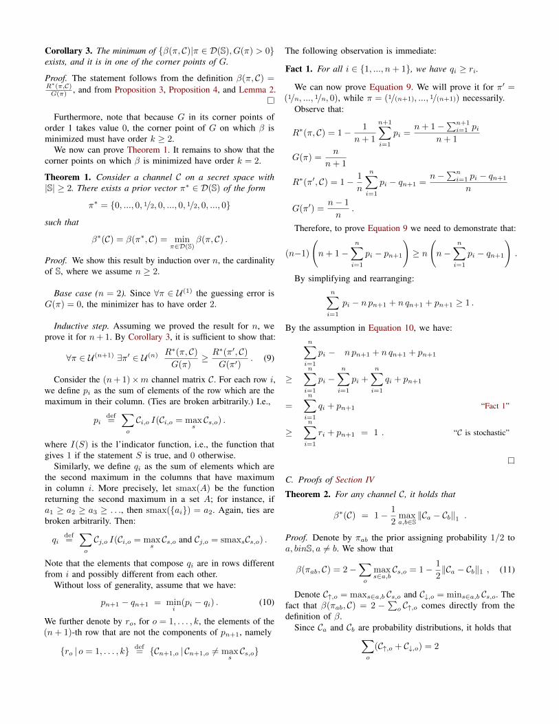
Corollary 3. The minimum of {β(π, C)|π ∈ D(S), G(π) > 0}exists, and it is in one of the corner points of G.

Proof. The statement follows from the definition β(π, C) =R∗(π,C)G(π) , and from Proposition 3, Proposition 4, and Lemma 2.

Furthermore, note that because G in its corner points oforder 1 takes value 0, the corner point of G on which β isminimized must have order k ≥ 2.

We now can prove Theorem 1. It remains to show that thecorner points on which β is minimized have order k = 2.

Theorem 1. Consider a channel C on a secret space with|S| ≥ 2. There exists a prior vector π∗ ∈ D(S) of the form

π∗ = {0, ..., 0, 1/2, 0, ..., 0, 1/2, 0, ..., 0}

such that

β∗(C) = β(π∗, C) = minπ∈D(S)

β(π, C) .

Proof. We show this result by induction over n, the cardinalityof S, where we assume n ≥ 2.

Base case (n = 2). Since ∀π ∈ U (1) the guessing error isG(π) = 0, the minimizer has to have order 2.

Inductive step. Assuming we proved the result for n, weprove it for n+ 1. By Corollary 3, it is sufficient to show that:

∀π ∈ U (n+1) ∃π′ ∈ U (n) R∗(π, C)G(π)

≥ R∗(π′, C)G(π′)

. (9)

Consider the (n+ 1)×m channel matrix C. For each row i,we define pi as the sum of elements of the row which are themaximum in their column. (Ties are broken arbitrarily.) I.e.,

pidef=∑o

Ci,o I(Ci,o = maxsCs,o) .

where I(S) is the l’indicator function, i.e., the function thatgives 1 if the statement S is true, and 0 otherwise.

Similarly, we define qi as the sum of elements which arethe second maximum in the columns that have maximumin column i. More precisely, let smax(A) be the functionreturning the second maximum in a set A; for instance, ifa1 ≥ a2 ≥ a3 ≥ . . ., then smax({ai}) = a2. Again, ties arebroken arbitrarily. Then:

qidef=∑o

Cj,o I(Ci,o = maxsCs,o and Cj,o = smaxsCs,o) .

Note that the elements that compose qi are in rows differentfrom i and possibly different from each other.

Without loss of generality, assume that we have:

pn+1 − qn+1 = mini

(pi − qi) . (10)

We further denote by ro, for o = 1, . . . , k, the elements of the(n+ 1)-th row that are not the components of pn+1, namely

{ro | o = 1, . . . , k} def= {Cn+1,o | Cn+1,o 6= max

sCs,o}

The following observation is immediate:

Fact 1. For all i ∈ {1, ..., n+ 1}, we have qi ≥ ri.

We can now prove Equation 9. We will prove it for π′ =(1/n, ..., 1/n, 0), while π = (1/(n+1), ..., 1/(n+1)) necessarily.

Observe that:

R∗(π, C) = 1− 1

n+ 1

n+1∑i=1

pi =n+ 1−

∑n+1i=1 pi

n+ 1

G(π) =n

n+ 1

R∗(π′, C) = 1− 1

n

n∑i=1

pi − qn+1 =n−

∑ni=1 pi − qn+1

n

G(π′) =n− 1

n.

Therefore, to prove Equation 9 we need to demonstrate that:

(n−1)

(n+ 1−

n∑i=1

pi − pn+1

)≥ n

(n−

n∑i=1

pi − qn+1

).

By simplifying and rearranging:n∑i=1

pi − n pn+1 + n qn+1 + pn+1 ≥ 1 .

By the assumption in Equation 10, we have:n∑i=1

pi − n pn+1 + n qn+1 + pn+1

≥n∑i=1

pi −n∑i=1

pi +

n∑i=1

qi + pn+1

=

n∑i=1

qi + pn+1 “Fact 1”

≥n∑i=1

ri + pn+1 = 1 . “C is stochastic”

C. Proofs of Section IV

Theorem 2. For any channel C, it holds that

β∗(C) = 1− 1

2maxa,b∈S

‖Ca − Cb‖1 .

Proof. Denote by πab the prior assigning probability 1/2 toa, binS, a 6= b. We show that

β(πab, C) = 2−∑o

maxs∈a,b

Cs,o = 1− 1

2‖Ca − Cb‖1 , (11)

Denote C↑,o = maxs∈a,b Cs,o and C↓,o = mins∈a,b Cs,o. Thefact that β(πab, C) = 2 −

∑o C↑,o comes directly from the

definition of β.Since Ca and Cb are probability distributions, it holds that∑

o

(C↑,o + C↓,o) = 2

Hence, we have that

‖Ca − Cb‖1 =∑o

(C↑,o − C↓,o) = 2∑o

C↑,o − 2

and (11) follows directly. We conclude by Theorem 1.

We now show that taking convex combinations of vectorscannot increase the diameter of a set, which will be useful forboth Proposition 1 and Theorem 4. Denote by diam(S), ch(S)the diameter and the convex hull of S respectively.

Lemma 3. For any S ⊆ Rn, it holds that

diam(ch(S)) = diam(S),

where distances are measured wrt any norm ‖ · ‖.

Proof. Let d = diam(S). Since S ⊆ ch(S) we clearly haved ≤ diam(ch(S)), the non-trivial part is to show that d ≥diam(ch(S)).

We first show that

∀a ∈ S, b ∈ ch(S) : ‖a− b‖ ≤ d . (12)

Let a ∈ S, b ∈ ch(S) and denote by Bd[a] the closed ball ofradius d centered at a. The diameter of S is d, hence

Bd[a] ⊇ S , and since balls are convexBd[a] = ch(Bd[a]) ⊇ ch(S) ,

which implies ‖a− b‖ ≤ d.Finally we show that

∀b, b′ ∈ ch(S) : ‖b− b′‖ ≤ d .

Let b, b′ ∈ ch(S), from (12) we know that Bd[b] ⊇ S, andsince balls are convex we have that Bd[b] ⊇ ch(S), whichimplies ‖b− b′‖ ≤ d.

Proposition 1. Let C be a channel, q ∈ D(O), and d =maxs∈S ‖Cs − q‖1. Then 1 − d ≤ β∗(C) . Moreover, if q ∈ch(CS) then β∗(C) ≤ 1− d/2 .

Proof. Let s, s′ ∈ S, from the triangle inequality we have that

‖Cs − C′s‖1 ≤ ‖Cs − q‖1 + ‖C′s − q‖1 ,

hence diam(CS) ≤ 2d and the lower bound follows fromTheorem 2.

Moreover, assume that q ∈ ch(CS). Since Cs ∈ ch(CS) forall s ∈ S, it holds that

diam(ch(CS)) ≥ maxs∈S‖Cs − q‖1 = d .

From Lemma 3 we get that

diam(CS) = diam(ch(CS)) ≥ d ,

which gives us an upper bound from Theorem 2.

D. Proofs of Section V

Theorem 3. For all channels C1, C2 it holds that

β∗(C1||C2) ≥ β∗(C1) · β∗(C2) .

Proof. Recall that πab ∈ D(S) denotes the prior that assignsprobability 1/2 to both a, b ∈ S, a 6= b. We will use the factthat for such priors, β(πab, C) can be written as

β(πab, C) =∑o∈O

mins∈{a,b}

Cs,o . (13)

This comes from the definition of β and the fact that the rowsCa and Cb are probability distributions, hence

(∑o∈O

mins∈{a,b}

Cs,o) + (∑o∈O

maxs∈{a,b}

Cs,o) =∑o∈O

∑s∈{a,b}

Cs,o = 2 .

We also use the basic fact that for non-negative {qi, ri}i:

(miniqi) · (min

iri) ≤ min

i(qi · ri) (14)

The proof proceeds as follows:

β∗(C1)β∗(C2)=

(mina,b∈S

β(πab, C1))(

mina,b∈S

β(πab, C2))

“Theorem 1”

≤ mina,b∈S

(β(πab, C1) · β(πab, C2)

)“(14)”

= mina,b∈S

( ∑o1∈O1

mins∈{a,b}

C1s,o1)( ∑

o2∈O2

mins∈{a,b}

C2s,o2)

“(13)”

=

mina,b∈S

∑o1∈O1

∑o2∈O2

(min

s∈{a,b}C1s,o1

)(min

s∈{a,b}C2s,o2)

)“Rearranging sums, distributivity”

≤ mina,b∈S

∑o1∈O1

∑o2∈O2

mins∈{a,b}

C1s,o1C2s,o2 “(14)”

= mina,b∈S

∑o∈O1×O2

mins∈{a,b}

(C1||C2)s,o “Def. of C1||C2”

= mina,b∈S

β(πab, C1||C2) “(13)”

= β∗(C1||C2)

Theorem 4. For all channels C1, C2 it holds that

β∗(C1C2) ≥ max{β∗(C1), β∗(C2)} .

Proof. The β∗(C1C2) ≥ β∗(C1) part is easy, and comes fromthe fact that

R∗(π, C1C2) ≥ R∗(π, C1)

for all priors π, hence also for the one achieving β∗(C1C2).The more interesting part is to show that β∗(C1C2) ≥ β∗(C2).

The key observation is that the rows of C1C2 are convexcombinations of those of C2:

(C1C2)s1 =∑s2∈S2

C1s1,s2C2s2 for all s1 ∈ S1

Denote by CS = {Cs | s ∈ S} the set of C’s rows, we have:

(C1C2)S1 ⊆ ch(C2S2) , hence

diam((C1C2)S1) ≤ diam(ch(C2S2)) .

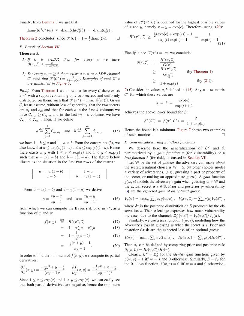
Finally, from Lemma 3 we get that

diam((C1C2)S1) ≤ diam(ch(C2S2)) = diam(C2S2) .

Theorem 2 concludes, since β∗(C) = 1− 12diam(CS).

E. Proofs of Section VII

Theorem 5.1) If C is ε-LDP, then for every π we have

β(π, C) ≥ 21+exp(ε) .

2) For every n,m ≥ 2 there exists a n×m ε-LDP channelC∗ such that β∗(C∗) = 2

1+exp(ε) . Examples of such C∗’sare illustrated in Figure 7.

Proof. From Theorem 1 we know that for every C there existsa π∗ with a support containing only two secrets, and uniformlydistributed on them, such that β∗(π∗) = minπ β(π, C). GivenC, let us assume, without loss of generality, that the two secretsare s1 and s2, and that for each o in the first k columns wehave Cs1,o ≥ Cs2,o, and in the last m − k columns we haveCs1,o < Cs2,o. Then, if we define

adef=

k∑j=1

Cs1,oj and bdef=

m∑j=k+1

Cs2,oj , (15)

we have 1− b ≤ a and 1−a < b. From the constraints (3), wealso know that a ≤ exp(ε)(1−b) and b ≤ exp(ε)(1−a). Hencethere exists x, y with 1 ≤ x ≤ exp(ε) and 1 < y ≤ exp(ε)such that a = x(1 − b) and b = y(1 − a). The figure belowillustrates the situation in the first two rows of the matrix:

a = x (1− b) 1− a1− b b = y (1− a)

From a = x(1− b) and b = y(1− a) we derive

a =xy − xxy − 1

and b =xy − yxy − 1

, (16)

from which we can compute the Bayes risk of C in π∗, as afunction of x and y:

f(x, y)def= R∗(π∗, C) (17)= 1− π∗s1a− π

∗s2b (18)

= 1− 1

2(a+ b) (19)

=12 (x+ y)− 1

xy − 1. (20)

In order to find the minimum of f(x, y), we compute its partialderivatives:

∂f

∂x(x, y) =

− 12y

2 + y − 12

(xy − 1)2,

∂f

∂y(x, y) =

− 12x

2 + x− 12

(xy − 1)2.

Since 1 ≤ x ≤ exp(ε) and 1 < y ≤ exp(ε), we can easily seethat both partial derivatives are negative, hence the minimum

value of R∗(π∗, C) is obtained for the highest possible valuesof x and y, namely x = y = exp(ε). Therefore, using (20):

R∗(π∗, C) ≥12 (exp(ε) + exp(ε))− 1

exp(ε) exp(ε)− 1=

1

exp(ε)− 1.

(21)

Finally, since G(π∗) = 1/2, we conclude:

β(π, C) =R∗(π, C)G(π)

≥ R∗(π∗, C)G(π∗)

(by Theorem 1)

≥ 2

1 + exp(ε)(by (21)).

2) Consider the values a, b defined in (15). Any n×m matrixC∗ for which these values are

a = b =exp(ε)

exp(ε) + 1

achieves the above lower bound for β:

β∗(C∗) = β(π∗, C∗) =2

1 + exp(ε)

Hence the bound is a minimum. Figure 7 shows two examplesof such matrices.

F. Generalization using gain/loss functions

We describe here the generalizations of L× and β,parametrized by a gain function g (for vulnerability) or aloss function ` (for risk), discussed in Section VII.

Let W be the set of guesses the adversary can make aboutthe secret; a natural choice is W = S, but other choices modela variety of adversaries, (e.g., guessing a part or property ofthe secret, or making an approximate guess). A gain functiong(w, s) models the adversary’s gain when guessing w ∈W andthe actual secret is s ∈ S. Prior and posterior g-vulnerability[3] are the expected gain of an optimal guess:

Vg(π) = maxw∑s πsg(w, s) , Vg(π, C) =

∑o p(o)Vg(δ

o) ,

where δo is the posterior distribution on S produced by the ob-servation o. Then g-leakage expresses how much vulnerabilityincreases due to the channel: L×g (π, C) = Vg(π, C)/Vg(π).

Similarly, we use a loss function `(w, s), modelling how theadversary’s loss in guessing w when the secret is s. Prior andposterior `-risk are the expected loss of an optimal guess:

R`(π) = minw∑s πs`(w, s) , R`(π, C) =

∑o p(o)R`(δ

o) .

Then β` can be defined by comparing prior and posterior risk:β`(π, C) = R`(π, C)/R`(π).

Clearly, L× = L×g for the identity gain function, given byg(w, s) = 1 iff w = s and 0 otherwise. Similarly, β = β` forthe 0-1 loss function, `(w, s) = 0 iff w = s and 0 otherwise.