The B.E. Journal of Macroeconomics - TAUalexcuk/pdf/Cukierman-Muscatelli_B.E.J.M._Issue_1... · The B.E. Journal of Macroeconomics Contributions Volume 8, Issue 1 2008 Article 7 Nonlinear

The B.E. Journal of Macroeconomics

Contributions

Volume8, Issue1 2008 Article 7

Nonlinear Taylor Rules and AsymmetricPreferences in Central Banking: Evidencefrom the United Kingdom and the United

States

Alex Cukierman∗ Anton Muscatelli†

∗Tel-Aviv University, [email protected]†Heriot-Watt University, [email protected]

Recommended CitationAlex Cukierman and Anton Muscatelli (2008) “Nonlinear Taylor Rules and Asymmetric Prefer-ences in Central Banking: Evidence from the United Kingdom and the United States,”The B.E.Journal of Macroeconomics: Vol. 8: Iss. 1 (Contributions), Article 7.Available at: http://www.bepress.com/bejm/vol8/iss1/art7

Copyright c©2008 The Berkeley Electronic Press. All rights reserved.

Nonlinear Taylor Rules and AsymmetricPreferences in Central Banking: Evidencefrom the United Kingdom and the United

States∗

Alex Cukierman and Anton Muscatelli

Abstract

This paper explores theoretically and empirically the view that Taylor rules are often nonlin-ear due to asymmetric central bank preferences, and that the nature of these asymmetries changesacross different policy regimes. The theoretical model uses a standard new Keynesian frameworkto establish equivalence relations between the shape of nonlinearities in Taylor rules and asym-metries in monetary policy objectives. These relations are estimated and tested for the UnitedKingdom (UK) and the United States (US) over various subperiods by means of smooth transitionregressions.

There is often evidence in favor of nonlinear rules in both countries, and their character changessubstantially over subperiods. The period preceding inflation targeting in the UK is characterizedby a concave rule supporting dominant recession avoidance preferences, while the inflation target-ing period is characterized by a convex rule supporting dominant inflation avoidance preferenceson the part of policymakers. Dominant inflation avoidance appears during the Vietnam War inthe US while, during the Burns/Miller and the Greenspan periods, recession avoidance dominates.Under Volcker the Taylor rule is linear. This is consistent with an offset by inflation avoidance ofthe more prevalent recession avoidance of the Fed.

Findings from both countries support the view that reaction functions and the asymmetry proper-ties of the underlying loss functions change in line with the regime and the main macroeconomicproblem of the day.

KEYWORDS: Taylor rules, nonlinearities, central banks, asymmetric preferences, recession avoid-ance, inflation avoidance, UK, US

∗Tel-Aviv University, and CEPR ([email protected]) and Heriot-Watt University and CESifo([email protected]) respectively. We benefited from the detailed suggestions of two anony-mous referees and of the editor, David Romer, as well as from the reactions of Petra Geraats and ofparticipants at the macro lunch seminar at Princeton University. This paper grew out of the paper:“Do Central Banks have Precautionary Demands for Expansions and for Price Stability? A NewKeynesian Approach” (Cukierman and Muscatelli, 2003).

1 Introduction

The positive theory of monetary policy in developed economies has reached abroad consensus in recent years. Monetary policy is conceptualized as follows:policy authorities minimize a linear combination of the quadratic deviationsof in�ation and of output from their respective targets (the in�ation and theoutput gaps in what follows), and the main policy instrument is the short-termrate of interest.1 Much of the literature of the last decade has implementedthis perspective by estimating Taylor rules or reaction functions, in which theshort-term rate is a linear function of the (currently expected) future valuesof the in�ation and of the output gaps.2 It is well known that, as a theoreticalmatter, such linear reaction functions are obtained when the expected value ofa loss function that is quadratic in the in�ation and output gaps is minimized,subject to a linear economic structure.

More recently, some of the literature has considered the possibility that,as a positive matter, the loss function of monetary policymakers may not bequadratic and consequently the Taylor rules derived from such functions arenot necessarily linear. There is both anecdotal and systematic evidence tosupport this view. On the anecdotal side, Blinder (1998, pp. 19, 20) states that"In most situations the central bank will take far more political heat when ittightens preemptively to avoid higher in�ation than when it eases preemptivelyto avoid higher unemployment." This suggests that during normal times thecentral bank (CB) in the United States may be more averse to negative thanto positive output gaps.3 We refer to CB loss functions that display this typeof asymmetry as recession-avoidance preferences (RAP). In the presence ofuncertainty about future shocks, such asymmetry leads the CB to take moreprecautions against negative than against positive output gaps.

Using a natural-rate framework and time-series data for the UnitedStates (US), Ruge-Murcia (2003) tests this hypothesis empirically and �nds

1This obviously includes strict in�ation targeting as the particular case in which theweight on the output gap is equal to zero.

2A partial list of references includes Clarida et al. (1998, 2000), Muscatelli et al. (2002),and Muscatelli and Trecroci (2002).

3In fact, notwithstanding its analytical convenience, a quadratic loss function that pe-nalizes equally sized positive and negative output gaps to the same extent does not appearto be realistic. Obviously, policymakers are averse to negative output gaps, but it is less ob-vious that, given in�ation, they are equally averse to positive output gaps. They may even,given in�ation, be indi¤erent to di¤erent magnitudes of positive output gaps. Cukierman(2000, 2002) shows that in the last case, and in the presence of uncertainty and rational ex-pectations there is an in�ation bias even if the output target of the CB is equal to potentialoutput.

1

Cukierman and Muscatelli: Nonlinear Taylor Rules and Asymmetric Preferences: UK and US

Published by The Berkeley Electronic Press, 2008

that it provides a better explanation for the behavior of US in�ation than theKydland-Prescott (1977) and the Barro-Gordon (1983) in�ation bias models.Using a natural-rate framework and cross-sectional data for the OECD coun-tries, Cukierman and Gerlach (2003) �nd evidence supporting a half quadraticspeci�cation of output-gap losses.4

On the other hand, during periods of in�ation stabilization in whichmonetary policymakers are trying to build up credibility, they may be moreaverse to positive than to negative in�ation gaps of equal size. We refer toobjective functions that display this type of asymmetry as in�ation-avoidancepreferences (IAP). In the presence of uncertainty about future shocks policy-makers with such preferences tend to react more vigorously to positive thanto negative in�ation gaps. Although there is no current systematic evidenceto support such a view, this might have been the case in the United Kingdomfollowing the introduction of in�ation targets in 1992 and during the gradualIsraeli disin�ation in the second half of the Nineties.5

Asymmetric objectives normally lead to nonlinear reaction functions.This paper utilizes time-series data from the United Kingdom (UK) and theUS to test whether there is evidence to support the view that the interest-rate reaction functions in those two countries exhibit nonlinearities, therebypointing to asymmetric policy preferences.

To understand the meaning of such nonlinearities for the loss functionsof UK and US monetary policymakers, in section 2, we provide a generalformulation of preferences in which recession avoidance and in�ation avoidancecoexist. We then analyze the character of nonlinearity in the Taylor rulesthat emerge. This is done for a new Keynesian economic structure of thetype surveyed in Clarida et al. (1999). The main theoretical implication isthat, when recession-avoidance preferences dominate, the reaction function isconcave in both the output and in�ation gaps, and when in�ation-avoidancepreferences dominate, the reaction function is convex in both gaps. This resultsuggests that we may expect to �nd di¤erent patterns of nonlinearities betweennormal periods and periods of credibility building.

4In this speci�cation, losses from negative output gaps are quadratic and, given in�ation,there are no losses from positive output gaps.

5During this period the in�ation target in Israel was missed much more frequently frombelow than from above, lending credence to the view that the Bank of Israel took moreprecautions against upward than against downward deviations from the target. Nobayand Peel (1998) and Ruge-Murcia (2000) show that in such cases a de�ationary bias mayarise. Mishkin and Posen (1997) express a similar view for in�ation targeters. A somewhatdi¤erent view appears in Sussman (2007), who interprets the Israeli experience to imply thatthe Bank of Israel pursued an implicit in�ation target lower than that set by the government.

2

The B.E. Journal of Macroeconomics, Vol. 8 [2008], Iss. 1 (Contributions), Art. 7

http://www.bepress.com/bejm/vol8/iss1/art7

Section 3 provides an empirical test of these hypotheses by allowingthe response of the interest rate to the expected values of both gaps to changegradually with the magnitude of each expected gap. This speci�cation, follow-ing Bacon and Watts (1971) and Seber and Wild (1989), utilizes hyperbolictangents to formulate the responses of the interest rate to the expected val-ues of the in�ation and output gaps. When the response increases with theexpected gap, the reaction function is convex in the expected gap; and whenthe response decreases in the expected gap, the reaction function is concave inthis gap. An important advantage of this speci�cation is that the concavity-convexity properties of the reaction function depend on only two parametersthat can be estimated by means of the same GMM methods used to estimatelinear Taylor rules.

When applied to appropriate subperiods, in the UK and the US, thismethodology yields several main results.6 First, in both the UK and the USnon-linear Taylor rules are more prevalent than linear rules. Second, the typeof nonlinearity changes between subperiods. In particular, the nonlinear Taylorrule for the UK in the 1979-1990 period is concave while the one for the 1992-2005 period is convex. This supports the view that prior to the introductionof in�ation targeting in 1992, RAP dominated; whereas after the introductionof in�ation targets, when stabilization of in�ation became a prime objectiveof policy, IAP became dominant.

Third, except for the period under Volcker�s chairmanship, the Fed�sreactions function are all nonlinear. Fourth, the character of those nonlinear-ities varies substantially across di¤erent US Fed chairs. In particular, whilethe Martin in�ationary period is characterized by convexity, the Taylor rule isconcave under Greenspan. This lends support to the view that when in�ationand in�ationary expectations were on the rise during the second half of theSixties, in�ation aversion dominated policy preferences. On the other hand,after in�ation had been conquered by Volcker, recession aversion became dom-inant under Greenspan. Finally, there is weaker, but still signi�cant, evidenceof dominant recession-avoidance preferences during the Burns/Miller era.

More generally, results from both countries support the view that thedominant type of asymmetry in monetary policy (recession avoidance versusin�ation avoidance) often changes with the economic environment.

6Our available sample period is 1979-3 to 2005-4 for the UK and 1960-1 to 2005-4 forthe US.

3



2 The relation between recession and in�ationavoidance preferences and the character ofnonlinearities in Taylor rules

Nonlinear reaction functions may arise because the loss functions of centralbankers are not quadratic, or because the economic structure is nonlinear, orfor both reasons. In this paper we focus on the �rst class of reasons for non-linearities in Taylor rules, by maintaining the assumption that the economicstructure is linear.7

To motivate the analysis of this section, consider the case in which theloss function of the CB displays RAP, causing the bank to be more averse tonegative than to positive output gaps of equal size. In the face of uncertainty,this type of asymmetry should induce the CB to try to lean more heavilyagainst negative than against positive output gaps, implying that the interest-rate response to an expected change in the gap should be weaker at positivethan at negative output gaps. Provided the aversion to output gaps weakensgradually as the size of the gap increases, intuition would suggest that in thepresence of RAP, the reaction function should be concave with respect to theoutput gap.

Similarly, the loss function could also display IAP in the sense thatpositive in�ation gaps are more costly than negative in�ation gaps of the samesize. IAP induce the CB to lean more heavily against positive than againstnegative in�ation gaps. If opposition to the in�ation gap weakens graduallyas the size of the gap decreases, intuition would suggest that in the presenceof in�ation avoidance, the CB will react more strongly to a change in in�ationwhen the size of this gap is higher. Hence the reaction function should beconvex with respect to the in�ation gap.

This section illustrates and rigorously con�rms this broad intuition fora new Keynesian economic structure of the type proposed by Clarida et al.(1999). This is done by deriving the interest-rate reaction function of a CBwhose loss function is characterized by both recession and in�ation avoidancepreferences. The analysis includes cases in which there is only recession avoid-ance or only in�ation avoidance, as particular cases. This formulation has twoadvantages. First it establishes the concavity/convexity properties of the re-action function with respect to both gaps rather than only with respect to the

7Dolado et al. (2004) �nd that there is no evidence against a linear aggregate supplyschedule for the US. A discussion of our �ndings within a broader perspective entertainingthe possibility of nonlinear Phillips curves appears at the end of the concluding section.

4



gap that is subject to an avoidance motive. Second, it allows both avoidancemotives to operate simultaneously. This provides a convenient framework forthe interpretation of estimated nonlinear reaction functions in section 3. Wenow turn to the details of the analysis.

2.1 General speci�cation of in�ation and recessionavoidance preferences

The objective of the monetary authority is to minimize

E0

1Xt=0

�tLt; (1)

where � is the discount factor and Lt is given by equation (2):

Lt = Af(xt) + h(�t � ��): (2)

Here A is a positive coe¢ cient, xt is the output gap, �t is in�ation, �� is thein�ation target and the functions f(xt) and h(�t � ��) possess the followingproperties:

f 0(xt) < 0 for xt < 0; f0(xt) � 0 for xt � 0; f(0) = f 0(0) = 0;

f 00(xt) > 0; f 000(xt) � 0;h0(�t � ��) � 0 for �t � �� 0; h0(�t � ��) > 0 for �t � �� > 0;

h(0) = h0(0) = 0; h00(�t � ��) > 0; h000(�t � ��) � 0; (3)

where the tags attached to the functions f(xt) and h(�t��) designate partialderivatives whose order is given by the number of tags. The speci�cation inequation (2) states that losses from both the output gap and the in�ation gapattain their minimal levels when those two gaps are zero and that losses arelarger, at least weakly, the larger the absolute value of the gaps. The �rst-orderpartial derivatives of both f(xt) and h(�t � ��) are zero when the gaps arezero. As with the quadratic, the second partial derivatives are assumed to bepositive, but unlike the quadratic f(xt) and h(�t��) need not be symmetricaround zero.

Potential asymmetries with respect to �nal objectives are introducedby means of assumptions on third partial derivatives. Stronger aversion tonegative than to positive output gaps (a RAP) is characterized by a nega-tive third derivative of the function, f(xt): A negative value of f 000(xt) means

5



that the rate at which the marginal loss of being away from potential outputchanges when this gap goes up, is decreasing in the output gap. In particularit implies that the marginal loss at a given negative output gap is larger thanthe marginal loss at a positive output gap with the same absolute value. 8

When f 000(xt) = 0; output gap losses are symmetric and there is no RAP. Thisis the standard quadratic case.

Analogously, stronger aversion to positive than to negative in�ationgaps (an IAP) is characterized by a positive third derivative of the functionh(�t � ��). A positive value of h000(�t � ��) means that the rate at which themarginal loss of deviating from the in�ation target changes when the in�ationgap goes up, is increasing in this gap. In particular, it implies that, for a givenabsolute value of the in�ation gap, the marginal cost of a positive deviationfrom the target is larger than the marginal cost of a negative deviation. Thiskind of asymmetry may arise during periods of in�ation stabilization in whichthe buildup of credibility is a primary consideration. In the particular caseh000(�t � ��) = 0; in�ation gap losses are symmetric and there is no IAP.9

2.2 Economic structure

The behavior of the economy is characterized by means of a stylized purelyforward looking new Keynesian, sticky prices framework, presented in Claridaet al. (1999) and is brie�y summarized in what follows.10 Within this frame-work, in�ation depends on the currently expected future in�ation and on the

8There is a formal analogy between this formulation of recession aversion and the for-mulation of utility of a consumer possessing a precautionary demand for savings. Kimball(1990) shows that a necessary and su¢ cient condition for the existence of the latter is thatthe marginal utility of consumption or income be a convex function of income (a positivethird partial derivative). Similarly, the condition �f 000(xt) > 0; that characterizes recessionavoidance, means that the marginal utility, to policymakers, of an increase in output is aconvex function of output. However, the analogy is only partial since the precautionarydemand for savings a¤ects the stock of savings while recession aversion a¤ects the interestrate chosen by the CB.

9Geraats (2006) utilizes a similar modeling of RAP (prudence in her terminology) toprovide an explanation for the relation between in�ation and its variability within a Barro-Gordon framework.10For the deeper motivation and assumptions underlying this well-known structure, the

reader is referred to the original article. The main theoretical proposition of this sectionis derived for this purely forward looking model since it allows analytical solutions thatestablish useful correspondences between di¤erent types of asymmetric objectives and thecurvature of the CB reaction function. However, the empirical work below also includes alagged interest-rate term in the reaction function to control for the observed sluggishness ofthe policy rate.

6



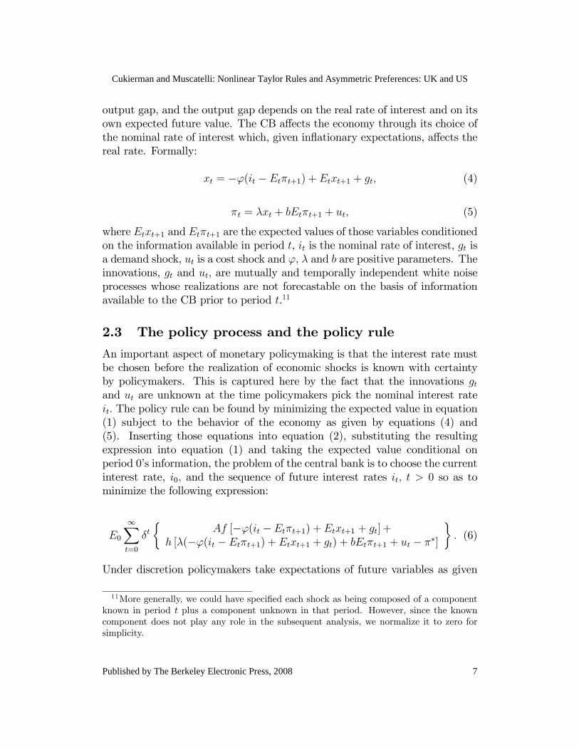
output gap, and the output gap depends on the real rate of interest and on itsown expected future value. The CB a¤ects the economy through its choice ofthe nominal rate of interest which, given in�ationary expectations, a¤ects thereal rate. Formally:

xt = �'(it � Et�t+1) + Etxt+1 + gt; (4)

�t = �xt + bEt�t+1 + ut; (5)

where Etxt+1 and Et�t+1 are the expected values of those variables conditionedon the information available in period t, it is the nominal rate of interest, gt isa demand shock, ut is a cost shock and '; � and b are positive parameters. Theinnovations, gt and ut; are mutually and temporally independent white noiseprocesses whose realizations are not forecastable on the basis of informationavailable to the CB prior to period t.11

2.3 The policy process and the policy rule

An important aspect of monetary policymaking is that the interest rate mustbe chosen before the realization of economic shocks is known with certaintyby policymakers. This is captured here by the fact that the innovations gtand ut are unknown at the time policymakers pick the nominal interest rateit: The policy rule can be found by minimizing the expected value in equation(1) subject to the behavior of the economy as given by equations (4) and(5). Inserting those equations into equation (2), substituting the resultingexpression into equation (1) and taking the expected value conditional onperiod 0�s information, the problem of the central bank is to choose the currentinterest rate, i0; and the sequence of future interest rates it; t > 0 so as tominimize the following expression:

E0

1Xt=0

�t�

Af [�'(it � Et�t+1) + Etxt+1 + gt] +h [�(�'(it � Et�t+1) + Etxt+1 + gt) + bEt�t+1 + ut � ��]

�: (6)

Under discretion policymakers take expectations of future variables as given

11More generally, we could have speci�ed each shock as being composed of a componentknown in period t plus a component unknown in that period. However, since the knowncomponent does not play any role in the subsequent analysis, we normalize it to zero forsimplicity.

7



and reoptimize each period. Since there are no lags this problem can be brokendown into a series of separate one-period problems. The typical �rst-ordercondition for an internal maximum is therefore:

AEtf0[:] + �Eth

0[:] = 0; t = 0; 1; 2; ::: ; (7)

where the expectation Et is taken over the distributions of the innovations gtand ut (unknown in period t). Period t�s condition determines the interest ratechosen in that period as a function of the in�ation and output gaps expectedfor period t+1: Note that since policy is discretionary and neither the economicstructure nor the objective function contain lagged terms, the current choiceof interest rate does not a¤ect current expectations of future periods�in�ationand the output gap.12

2.4 Comparative statics

The �rst-order condition in equation (7) implicitly determines the optimalchoice of interest rate by the CB as a function of expected in�ation and ofthe expected output gap. Since, except for the general restrictions implied byrecession and in�ation avoidance preferences, the functional forms of f(:) andh(:) are not further restricted, it is generally not possible to solve explicitly forthe reaction function of the CB as in the quadratic case. However, it is stillpossible to derive some features of the reaction function, and their relationsto the two types of asymmetric preferences, by performing comparative staticexperiments.

Totally di¤erentiating the �rst order condition for t = 0 in (7) withrespect to E0�1 and rearranging:

di0dE0�1

=1

'

'AE0f00

0 [:] + �('�+ b)E0h000 [:]

AE0f00

0 [:] + �2E0h000 [:]

� 'AE0f00

0 [:] + �('�+ b)E0h000 [:]

'D;

(10)

12This can be seen by taking expected values, as of t; of the economic structure in equations(4) and (5) which yields

Etxt+1 = �'(Etit+1 � Et�t+2) + Etxt+2 + Etgt+1; (8)

Et�t+1 = �Etxt+1 + bEt�t+2 + Etut+1: (9)

8



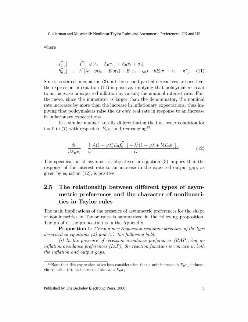
where

f00

0 [:] � f00[�'(i0 � E0�1) + E0x1 + g0];

h00

0 [:] � h00[�(�'(i0 � E0�1) + E0x1 + g0) + bE0�1 + u0 � ��]: (11)

Since, as stated in equation (3), all the second partial derivatives are positive,the expression in equation (11) is positive, implying that policymakers reactto an increase in expected in�ation by raising the nominal interest rate. Fur-thermore, since the numerator is larger than the denominator, the nominalrate increases by more than the increase in in�ationary expectations, thus im-plying that policymakers raise the ex ante real rate in response to an increasein in�ationary expectations.

In a similar manner, totally di¤erentiating the �rst order condition fort = 0 in (7) with respect to E0x1 and rearranging13:

di0dE0x1

=1

'

A(1 + '�)E0f00

0 [:] + �2(1 + '�+ b)E0h000 [:]

D: (12)

The speci�cation of asymmetric objectives in equation (3) implies that theresponse of the interest rate to an increase in the expected output gap, asgiven by equation (12), is positive.

2.5 The relationship between di¤erent types of asym-metric preferences and the character of nonlineari-ties in Taylor rules

The main implications of the presence of asymmetric preferences for the shapeof nonlinearities in Taylor rules is summarized in the following proposition.The proof of the proposition is in the Appendix.

Proposition 1: Given a new Keynesian economic structure of the typedescribed in equations (4) and (5), the following hold:

(i) In the presence of recession avoidance preferences (RAP), but noin�ation avoidance preferences (IAP), the reaction function is concave in boththe in�ation and output gaps.

13Note that this expression takes into consideration that a unit increase in E0x1 induces,via equation (9), an increase of size � in E0�1:

9



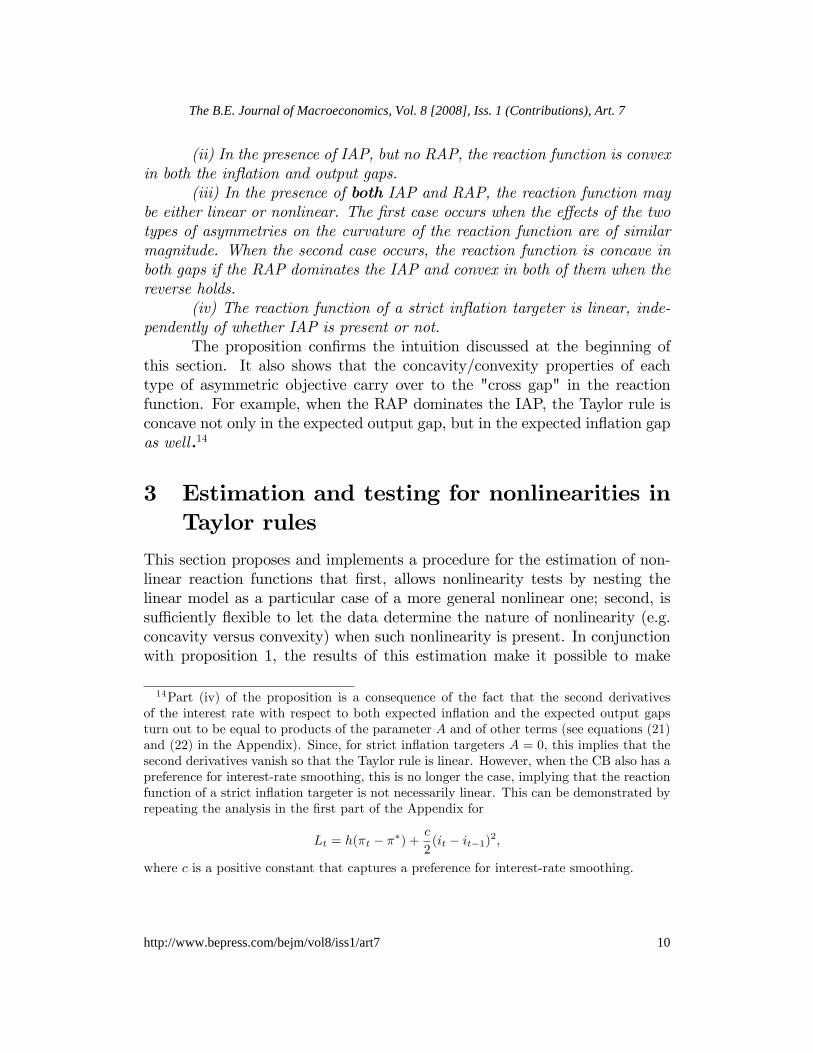
(ii) In the presence of IAP, but no RAP, the reaction function is convexin both the in�ation and output gaps.

(iii) In the presence of both IAP and RAP, the reaction function maybe either linear or nonlinear. The �rst case occurs when the e¤ects of the twotypes of asymmetries on the curvature of the reaction function are of similarmagnitude. When the second case occurs, the reaction function is concave inboth gaps if the RAP dominates the IAP and convex in both of them when thereverse holds.

(iv) The reaction function of a strict in�ation targeter is linear, inde-pendently of whether IAP is present or not.

The proposition con�rms the intuition discussed at the beginning ofthis section. It also shows that the concavity/convexity properties of eachtype of asymmetric objective carry over to the "cross gap" in the reactionfunction. For example, when the RAP dominates the IAP, the Taylor rule isconcave not only in the expected output gap, but in the expected in�ation gapas well .14

3 Estimation and testing for nonlinearities inTaylor rules

This section proposes and implements a procedure for the estimation of non-linear reaction functions that �rst, allows nonlinearity tests by nesting thelinear model as a particular case of a more general nonlinear one; second, issu¢ ciently �exible to let the data determine the nature of nonlinearity (e.g.concavity versus convexity) when such nonlinearity is present. In conjunctionwith proposition 1, the results of this estimation make it possible to make

14Part (iv) of the proposition is a consequence of the fact that the second derivativesof the interest rate with respect to both expected in�ation and the expected output gapsturn out to be equal to products of the parameter A and of other terms (see equations (21)and (22) in the Appendix). Since, for strict in�ation targeters A = 0; this implies that thesecond derivatives vanish so that the Taylor rule is linear. However, when the CB also has apreference for interest-rate smoothing, this is no longer the case, implying that the reactionfunction of a strict in�ation targeter is not necessarily linear. This can be demonstrated byrepeating the analysis in the �rst part of the Appendix for

Lt = h(�t � ��) +c

2(it � it�1)2;

where c is a positive constant that captures a preference for interest-rate smoothing.

10



inferences about the dominant type of asymmetry, if any, and to examine itstemporal stability.

3.1 A linear benchmark

In the absence of asymmetries, the CB loss function is quadratic in both thein�ation and the output gaps. As is well known, this leads to linear reactionfunctions. In the presence of asymmetries the interest-rate reaction functionmay be nonlinear. As a benchmark, we start from linear reaction functionsof the type estimated by Clarida et al. (1998, 2000). In this type of reactionfunction the desired interest rate, i�t ; is given by

i�t = �+ �(E[�t;kjt]� ��) + E[xt;qjt]; (13)

where �� is the in�ation target, t is the information set of the CB in periodt, and E[�t;kjt] (and E[xt;qjt]) are the rate of in�ation (and the output gap)expected to materialize in period t + k (and t + q), given this informationset. In practice, it is commonly found that central banks adjust the policyrate gradually so that the actual rate converges to the desired rate through apartial adjustment mechanism (Clarida et al., 1998, 2000):15

it = �it�1 + (1� �)i�t : (14)

Combining equations (13) and (14) and adding an exogenous interest ratecontrol error, �t; yields

it = (1� �)f�+ �(E[�t;kjt]� ��) + E[xt;qjt]g+ �it�1 + �t: (15)

Adding and subtracting �E[�t;kjt] and E[xt;qjt] to equation (15) andrearranging:

it = (1� �)fe�+ ��t;k + xt;qg+ �it�1 + "t; (16)

where e� = � � �� and the error term, "t; is a linear combination of theforecast errors of in�ation and of the output gap, and of the interest rate

15For a justi�cation of interest-smoothing behavior, see Cukierman (1990, 1992). Svensson(2000) and Muscatelli et al. (2002) develop models that include the costs of interest-rateadjustment in the optimization exercise.

11



control error.16

We start by estimating the linear benchmark in equation (16).17 Es-timation is performed by means of Hansen�s (1982) Generalized Method ofMoments (GMM), using as instruments four lags of the policy targets (outputand in�ation) and four lags of the policy instrument (the interest rate) and ofthe real price of oil. Clarida et al. (op. cit.) experiment with various leads forthe output gap and expected in�ation, but in fact q = k = 1 seems to �t thedata reasonably well, and the estimates of the parameters are not too sensitiveto changes in q and k over the range of 1 to 4 quarters.

Information about the data used appears in part 4 of the appendix.18

The data used are quarterly, and the sample period is 1979-3 to 2005-4 for theUK and 1960-1 to 2005-4 for the US. The beginning of the sample in the US isdictated by data availability. In the case of the UK, the full sample is availablefrom about 1976, three years earlier than the start of our sample. We chosenot to utilize those additional three years of data and to start the UK samplein 1979, because in that year a Conservative government headed by MargaretThatcher replaced the previous Labour government and implemented a changein the monetary regime, with a switch toward an explicitly monetarist policy.

3.2 Parametrization of nonlinearities

To parametrize the nonlinearities, we focus on smooth-transition models (STR).Such models allow the marginal reaction of the short-term interest rate to ex-pected output and in�ation gaps to change smoothly over the range of thereaction function. STR naturally �t with the smooth speci�cation of recessionand in�ation avoidance preferences described in the previous section. Thisspeci�cation is based on the theory that it is unlikely that interest-rate re-sponses in the reaction function remain constant over a wide range and thenchange discontinuously at particular values of the in�ation or output gaps.

An STR model can be built following the modeling strategy proposed

16Its explicit form is "t = � [�(�t+k � E[�t;kjt]) + (xt+q � E[xt;qjt])]+�t: Here �t+kand xt+q are the actual values of in�ation and of the output gap in periods t+ k and t+ qrespectively.17We do not show these estimates here for reasons of space.18We use o¢ cial estimates of potential output from OECD and CBO sources to construct

series for the output gap. In contrast, Muscatelli et al. (2002) use estimates of the outputgap based on the Kalman �lter, to allow for gradual learning by the authorities of changesin the processes generating in�ation and the output gap. Using o¢ cial data on the outputgap makes our results more directly comparable to most of the existing empirical literatureon interest rate reaction functions.

12



by Granger and Terasvirta (1993). This method allows the coe¢ cients ofvariables that might enter nonlinearly to depend on a transition variable, zt;that governs the smooth transition. For example, one may parametrize themarginal response of the interest rate to future in�ation in equation (16) as

� = �1 + �2F (zt); (17)

where F (zt) is an appropriate nonlinear and continuous function of zt: A sim-ilar procedure can be applied to the coe¢ cient, ; of the future output gapin equation (16). Granger and Terasvirta propose either the logistic or ex-ponential functions to model the smooth transition. However, we obtained abetter �t by using a hyperbolic tangent (tanh) function to capture the gradualtransition of the marginal response.19 Following are the details of this para-metrization: Let yz(zt � �z) � z(zt � �z) be a linear function of zt where zand �z are parameters to be determined. The hyperbolic tangent of y(zt) isgiven by

F [yz(zt � �z)] = tanh [yz(zt � �z)] �eyz(:) � e�yz(:)

eyz(:) + e�yz(:): (18)

The hyperbolic tangent is a monotonically increasing function of yz(:): As yz(:)varies between minus and plus in�nity, tanh varies between -1 and +1. Wheny(:) = 0; tanh is zero and has an in�ection point at zero. For negative valuesof yz(:); tanh is convex and for positive values of yz(:); it is concave in yz(:):The additional sub-parametrization of yz(:) in terms of zt governs the locationand the spread of the hyperbolic tangent in terms of the transition variablezt: In particular, �z determines the location of the point of in�ection of tanh;and z determines how quickly it moves up with the transition variable zt.

The analysis in section 2 implies that the in�ation gap is an appropriatetransition variable for � and that the output gap is an appropriate transitionvariable for . This leads to the following extension of equation (16):

it = (1� �)fb�+ �1�t;1 + 1xt;1 + �2(�t;1 � ��) tanh [ �(�t;1 � ��)]

+ 2xt;1 tanh [ x(xt;1)]g+ �it�1 + "t��; (19)

where the explicit form of tanh is given in equation (18) and where we allow,in principle, for the possibility that the parameters and � vary, depending

19Such parametrization was proposed by Bacon and Watts (1971), and Seber and Wild(1989).

13



on whether the variable which determines the transition is the output gap orthe in�ation gap.20 More precisely, tanh [y�(�t;1 � ��)] = tanh [ �(�t;1 � ��)]and �x is constrained to zero so that tanh [yx(xt;1 � �x)] = tanh [ xxt;1] : How-ever, as explained later, the various models tried �t the data well with therestriction x = � = so that in the estimated models, the two gaps enterthe hyperbolic tangent function with the same linear coe¢ cient, :

To illustrate the consequences of this speci�cation for the total responsecoe¢ cients of in�ation and of the output gap consider, for example, the impliedbehavior of �: As in�ation varies around ��, the value of the hyperbolic tangentfunction varies between -1 and 1. For a concrete example, suppose that �� =4%, and that � = 1. At low in�ation rates (approximately 2% below thethreshold) the tanh function is close to its lower asymptote of -1, so the long-run response of the nominal interest rate to expected in�ation in this range isapproximately (�1 � �2). By contrast, at high in�ation rates (approximately2% above ��, i.e. at 6% in�ation) the tanh function is close to its upperasymptote of 1, so that the nominal interest rate response to expected in�ationin this range is approximately (�1+�2). In between, � is a monotonic functionof in�ation and is bounded between (�1 � �2) and (�1 + �2). Depending onwhether �2 is positive or negative, the marginal response of the interest rate toin�ation is (for the most part) an increasing or decreasing function of in�ation,implying that the coe¢ cient �2 determines whether the reaction function isconvex or concave in expected in�ation.21 Analogous considerations apply tothe response of the interest rate to the output gap.

Equation (19) is estimated by GMM for alternative values of the pa-rameter in the range between 0:1 and 1 with increments of 0:1: Since,in terms of goodness of �t, the best results are obtained, by and large, for x = � � = 0:2; all the results presented are for this common value of :Four lags of all the explanatory variables are used as instrumental variables inthe estimation. A convenient feature of the hyperbolic tangent smooth transi-tion regressions (HTSTR) is that they make it possible to estimate the implicitin�ation target, ��; along with the other parameters even in the absence of anexplicit in�ation target.

20b� � �� 1��:21The analytical details underlying this statement are set out in the second part of the

appendix.

14



3.3 Estimation procedures and results for the UK

Table 1 presents estimated HTSTR for the UK, for the subperiods 1979:3-1990:3 and 1992:4-2005:4.22 The beginning of the sample is chosen to coincidewith the beginning of the Conservative government under Margaret Thatcher.An explicit in�ation target had been announced by the UK government since1992. The breakdown of the sample into those two subperiods is meant tocapture potential di¤erences in the reaction function between the �rst period,in which there was no explicit target, and the second one which was character-ized by an explicitly announced in�ation target. For the �rst subperiod, theimplicit in�ation target is estimated along with the other parameters.23 Forthe second subperiod, the o¢ cially announced in�ation target (which is 2:5%in terms of the retail price index) was used.24

In both regressions the linear coe¢ cient, �1; on expected in�ation ispositive and signi�cant. The linear coe¢ cients, 1; on the output gap are alsopositive and signi�cant. All regressions display the commonly found gradualadjustment of the interest rate to the desired level with a non-adjustment co-e¢ cient that varies between 0.62 and 0.84. The coe¢ cient �2 that governsthe smooth transition in the case of expected in�ation is uniformly signi�-cant. The coe¢ cient, 2 that governs the smooth transition in the case of theexpected output gap is signi�cant only in the �rst subperiod. Interestingly,the linear coe¢ cients on expected in�ation are all substantially higher thanone. However, due to the nonlinearity of the Taylor rule, these coe¢ cients donot su¢ ce to establish whether the Taylor principle is satis�ed or not. To dothat we need to evaluate the total (nonlinear) response of the interest rate to

22The period 1990:4-1992:2 has been excluded from the subsamples since, during thisperiod, the UK belonged to the exchange rate mechanism of the EMS implying that UKmonetary policy at that time was largely shadowing that of the German Bundesbank. Wealso estimated an HTSTR for the entire period (excluding the period of the exchange ratemechanism) but after observing the dramatic di¤erences between the subperiods, decidednot to present it because it averages out two distinct behavioral patterns.23We estimate �� and using a grid search procedure to provide the best �t for the GMM

criterion function. As noted above, we found that = 0:2 provided the best �t throughoutand hence this is not tabulated.24In December 2003, the UK government changed the Bank of England�s in�ation target

from RPIX to the harmonised index of consumer prices (CPI), with a target of 2%. However,it is generally accepted that this new remit of a 2% target for CPI was, at the time, broadlyconsistent with a 2.5% target for RPIX.

15



in�ation.25 This response is given by

@i

@�t;1= �1+�2

htanh [ (�t;1 � ��)] + (�t;1 � ��) tanh

0[ (�t;1 � ��)]

i: (20)

where tanh0[:] is the �rst derivative of tanh with respect to its argument.

It is shown in the second part of the Appendix that for most of the rates ofin�ation experienced in the UK over the sample period, this response increases(decreases) with in�ation if and only if �2 is positive (negative). Consequently,the reaction function is convex or concave in expected in�ation, depending onwhether �2 is positive or negative.

26

Table 1Hyperbolic Tangent Smooth Transition Regressions (HTSTR):

UK, 1979 - 2005Estimated Coe¢ cients Stats

Period bb� b�1 b�2 b 1 b 2 b� ��

1979:3to

1990:31.99(3.88)

1.71��

(0.63)-0.76�

(0.42)0.88�

(0.54)-3.17�

(1.82)0.62��

(0.12)7.5

�=1.07J15=14.4

1992:4to

2005:44.46(4.92)

2.25�

(1.23)4.51��

(1.65)4.61��

(1.52)2.23(2.89)

0.84��

(0.05)2.5

�=0.35J15=18.1

Notes: Numbers in parentheses indicate standard errors (using a consistent covari-

ance matrix for heteroscedasticity and serial correlation); � indicates the standard error

of the regression; Jn is Hansen�s test of the model�s overidentifying restrictions, which is

distributed as a �2(n + 1) variate under the null hypothesis of valid overidentifying re-strictions (n represents the number of instruments minus the number of freely estimated

parameters). Two stars designate a coe¢ cient/statistic that is signi�cant at the 5% level,

and one star indicates signi�cance at the 10% level. The interest rate, the output gap,

in�ation, the in�ation target, ��; and � are all measured in percentages.

25Recall that, due to the features of the GMM estimation procedure, the coe¢ cients ofthe actual future in�ation rate are identical to the coe¢ cient of expected in�ation.26Similarly, part 3 of the Appendix shows that if 2 is positive (negative), the reaction

function is convex (concave) with respect to the expected output gap.

16



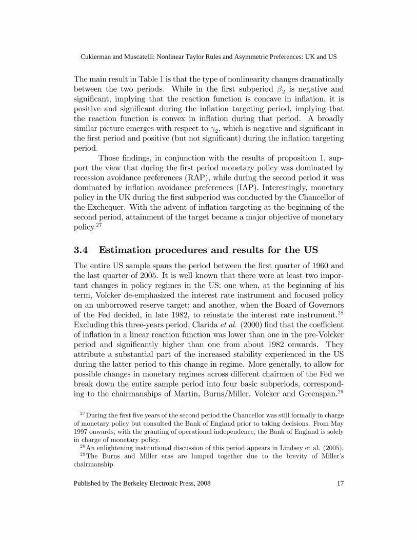
The main result in Table 1 is that the type of nonlinearity changes dramaticallybetween the two periods. While in the �rst subperiod �2 is negative andsigni�cant, implying that the reaction function is concave in in�ation, it ispositive and signi�cant during the in�ation targeting period, implying thatthe reaction function is convex in in�ation during that period. A broadlysimilar picture emerges with respect to 2; which is negative and signi�cant inthe �rst period and positive (but not signi�cant) during the in�ation targetingperiod.

Those �ndings, in conjunction with the results of proposition 1, sup-port the view that during the �rst period monetary policy was dominated byrecession avoidance preferences (RAP), while during the second period it wasdominated by in�ation avoidance preferences (IAP). Interestingly, monetarypolicy in the UK during the �rst subperiod was conducted by the Chancellor ofthe Exchequer. With the advent of in�ation targeting at the beginning of thesecond period, attainment of the target became a major objective of monetarypolicy.27

3.4 Estimation procedures and results for the US

The entire US sample spans the period between the �rst quarter of 1960 andthe last quarter of 2005. It is well known that there were at least two impor-tant changes in policy regimes in the US: one when, at the beginning of histerm, Volcker de-emphasized the interest rate instrument and focused policyon an unborrowed reserve target; and another, when the Board of Governorsof the Fed decided, in late 1982, to reinstate the interest rate instrument.28

Excluding this three-years period, Clarida et al. (2000) �nd that the coe¢ cientof in�ation in a linear reaction function was lower than one in the pre-Volckerperiod and signi�cantly higher than one from about 1982 onwards. Theyattribute a substantial part of the increased stability experienced in the USduring the latter period to this change in regime. More generally, to allow forpossible changes in monetary regimes across di¤erent chairmen of the Fed webreak down the entire sample period into four basic subperiods, correspond-ing to the chairmanships of Martin, Burns/Miller, Volcker and Greenspan.29

27During the �rst �ve years of the second period the Chancellor was still formally in chargeof monetary policy but consulted the Bank of England prior to taking decisions. From May1997 onwards, with the granting of operational independence, the Bank of England is solelyin charge of monetary policy.28An enlightening institutional discussion of this period appears in Lindsey et al. (2005).29The Burns and Miller eras are lumped together due to the brevity of Miller�s

chairmanship.

17



HTSTR models are estimated for each subperiod. Except for the Volcker era,there is some evidence in favor of nonlinearities in all periods.30 Since to thisday the US does not practice explicit in�ation targeting, �� is estimated, in thenonlinear cases, along with the other coe¢ cients. As for the UK, this is doneby using a grid search that minimizes the criterion function over ��. Table 2summarizes the estimation results. The eleven quarters under Volcker duringwhich the operational target was unborrowed reserves were excluded from theVolcker sample period.

Table 2 suggests that the reaction function of the Fed varied in a nonnegligible manner across di¤erent chairs. Particularly striking is the di¤erencebetween the Martin and Greenspan reaction functions. Although there isevidence of nonlinearity under both chairs, the forms of nonlinearity di¤er.The signi�cantly positive �2 and 2 coe¢ cients under Martin are consistentwith dominant IAP, whereas the negative signs of those coe¢ cients underGreenspan are indicative of dominant RAP.31

Martin had a reputation for leaning toward sound money. Thus afterthe 1957-58 recession, in response to criticism of insu¢ cient ease before theHouse Ways and Means Committee, he said: "I do want to point out that ineight years of experience in the Federal Reserve System, I am convinced thatour bias, if anything, has been on the side of too much money rather than toolittle" (Wood, 2005, p. 256). This reputation is broadly consistent with theevolution of in�ation and of the Federal Funds rate during the Sixties. Fromthe beginning of 1960 till mid-1966, in�ation �uctuated within a narrow rangearound 2 percent. It then rose above 4 percent in two subsequent quarters andreceded for a while. But when in�ation appeared to permanently establishitself above 4 percent during 1968 and 1969, the policy reaction was strong.Wood (op. cit., p. 353) notes that in December 1968 the discount rate wasraised to 5.5 percent, and in April 1969: "...after in�ation had jumped to 6.9in the �rst quarter, with unemployment steady near 4 percent, the Fed raisedthe discount rate to 6 percent, its highest since 1929, and increased reserverequirements."32

30The unrestricted HTSTR estimation for the (relatively short) Volcker years displayedconvergence problems and the estimates of �1; �2; 1and 2 were all insigni�cant �indicatingoverparametrization. However, when the nonlinear parameters �2 and 2 were restricted tozero, the GMM estimate of the reaction function converged and recovered the signi�cantlinear coe¢ cients that appear in Volcker�s row in Table 2.31Conditions on the magnitudes of the in�ation and of the output gaps under which this

statement is valid are elaborated in the second and third parts of the appendix. Thoseconditions are almost always satis�ed.32Although the estimate of �1 is negative during this period, the total marginal response

18



Table 2Reaction Functions by Board Chairs: US, 1960:1 - 2005:4

Period Estimated Coe¢ cients Statsbb� or be� b�1 b�2 b 1 b 2 b� ��

Martin1960:11970:1

5.76��

(1.52)-1.80�

(0.98)3.21��

(0.63)0.34��

(0.17)0.09��

(0.04)0.76��

(0.08)1.3

�=0.42J15=11.6

Burns/Miller1970:21979:3

1.42��

(0.72)0.86��

(0.09)0.08(0.72)

0.55��

(0.19)-0.90��

(0.45)0.42��

(0.13)3.2

�=0.85J15=14.0

Volcker1982:41987:3

0.16(1.31)

1.52��

(0.29)- 0.80��

(0.40)- 0.89��

(0.03)-

�=0.84J17=11.6

Green-span1987:42005:4

2.35(1.08)

1.01��

(0.36)-0.92(0.85)

0.88��

(0.12)-0.84��

(0.14)0.81��

(0.03)2.9

�=0.38J15=13.4

Notes: Numbers in parentheses indicate standard errors (using a consistent covari-

ance matrix for heteroscedasticity and serial correlation); � indicates the standard error ofthe regression; Jn is Hansen�s test of the model�s overidentifying restrictions, which is dis-

tributed as a �2(n+1) variate under the null hypothesis of valid overidentifying restrictions(n represent the number of instruments minus the number of freely estimated parameters).Two stars designate a coe¢ cient/statistic that is signi�cant at the 5% level, and one star

indicates signi�cance at the 10% level. The interest rate, the output gap, in�ation, the

in�ation target, ��; and � are all measured in percentages.

On the other hand Greenspan, whose chairmanship started in the af-termath of Volcker�s disin�ation, felt that he could devote more attention torecession avoidance which, during periods of relatively stable prices, is not sosurprising in view of the dual mandate of the Fed as expressed in the 1946 FullEmployment Act.

Although there is no evidence of nonlinearity in in�ation during theBurns/Miller era, 2 is negative and signi�cant pointing toward nonlinearitiesin the output gap and recession avoidance preferences. Furthermore, in linewith previous results, the coe¢ cient on in�ation is smaller than one. Those

of the interest rate to in�ation is positive and substantially larger than one for practicallyall in�ation rates experienced under Martin.

19



�nding are broadly consistent with Burns� (1979, p. 16) famous statementthat the role of the Fed is to continue "probing the limits of its freedom toundernourish in�ation." In view of the dominant in�ation avoidance underMartin, the Burns/Miller period appears odd at �rst blush since, in spite ofrising in�ation, it displays recession avoidance. Two (not mutually exclusive)explanations are that Burns was subject to heavier political pressures thanhis predecessor, and that during his tenure, in�ation was accompanied by areduction in the rate of growth and an increase in unemployment, while underMartin in�ation was accompanied by an expansion.33

There is no evidence of nonlinearities under Volcker but the (constant)coe¢ cient on in�ation is signi�cantly higher than one, as in Clarida et al.(2000). A possible interpretation is that under Volcker, the Fed�s preferencesdisplayed both recession avoidance as well as in�ation avoidance, and that thereaction function was linear because those two asymmetries o¤set each other(part (iii) of proposition 1). Since the Full Employment Act of 1946 the Fedpossesses a dual policy mandate. It is therefore likely that although RAP aredeeply rooted in the Fed�s mandate, o¤setting IAP developed when it becameapparent that in�ation had reached intolerable levels.

Using a Linex speci�cation for asymmetric objectives and combiningthe Burns/Miller sample period together with that of Martin, Surico (2007)�nds evidence in favor of RAP over the combined pre-Volcker period. Due topooling of the two sample periods, this result is not necessarily inconsistentwith ours for the Burns/Miller era. But our results suggest that, due to thedi¤erent character of nonlinearities under Martin and Burns/Miller, lumpingof those periods together is likely to be misleading. Surico also tests for non-linearities in the Volcker-Greenspan era lumped into one period and �nds noevidence in favor of non linearities. Although these �ndings are not inconsis-tent with ours for the Volcker period, they are inconsistent with the preferencefor recession avoidance we detect under Greenspan. Again, this di¤erence maybe due to the pooling of sub-samples.34 One advantage of pooling sub-samplesis that the sample periods are longer. But this has to be weighted against thesubstantial di¤erences in curvature of the reaction functions that we detect

33Vivid illustrations of the pressures exerted by Nixon on Burns appear in a summaryof conversations between them from recently released Nixon tapes. For example, followingBurns�warning about excessive liquidity during an October 1971 conversation in the OvalO¢ ce Nixon responds by stating that the liquidity problem is "just bullshit" (Abrams, 2006,P. 180). See also chapter 4 of Meltzer (Forthcoming, 2008).34Besides di¤erences in methodology (Linex versus HTSTR) and in de�nition of periods,

Surico�s measure of in�ation is based on the personal consumption expenditure de�ator,while ours is based on the CPI.

20



under di¤erent US chairs.

4 Conclusion

Using hyperbolic tangent smooth transition regressions (HTSTR), this paperproduces evidence in favor of nonlinearities in Taylor rules for the UK andthe US. Our estimates of the parameters characterizing those nonlinearitiessupport the following conclusions: During the pre-in�ation targeting period inthe UK, the Taylor rule is concave. Given a linear new Keynesian economy,this �nding is consistent with the existence of dominant recession avoidancepreferences (RAP). During the in�ation targeting period in the UK (from 1992on), the Taylor rule is convex, supporting the existence of dominant in�ationavoidance preferences (IAP). The UK �ndings suggest that the introductionof in�ation targeting in the UK was accompanied by a fundamental change inthe objectives of monetary policy, not only with respect to the average target,but also in terms of precautions taken to keep in�ation in check in the face ofuncertainty about the economy.

Excluding the Volcker period as Fed chair, the evidence supports the ex-istence of nonlinearities in US interest-rate reaction functions under all chairs.Under Martin the Taylor rule is convex, supporting a dominant IAP, whileunder Greenspan it is concave supporting a dominant RAP. These results areconsistent with the view that the dominant type of asymmetry changes withthe most pressing economic problem of the recent past. The latter part ofMartin�s term was characterized by rising in�ation and in�ationary expecta-tions, and a low rate of unemployment, due to the Vietnam war and increasesin various social expenditures. By contrast, Greenspan became chairman af-ter Volcker brought in�ation down. Consequently, Martin developed in�ationavoidance whereas Greenspan could focus on recession avoidance.35 In a sim-ilar vein, the UK results are consistent with the view that, in addition toa substantial reduction in the target, the advent of in�ation targeting, and

35Since in�ation intensi�ed further under Burns, this interpretation raises the question ofwhy the evidence shows that recession avoidance (rather than in�ation avoidance) dominatedwhen he was chair. Two likely reasons are that Burns was subject to stronger politicalpressures and that unemployment rose sharply under his watch. Another question is whydid in�ation creep up at the end of Martin�s term in spite of IAP. One reason is that heoverestimated the dampening impact of the 1968 tax surcharge on in�ation as did manyeconomists at the time. And by the time he recognized the mistake he was out of o¢ ce.Detailed discussions of these and related issues appear in chapter 4 of Meltzer (Forthcoming,2008).

21



latterly central bank independence, was associated with an increase in theimportance of IAP relatively to RAP.

In principle nonlinear reaction functions of the type estimated in thispaper may arise even in the absence of asymmetric objectives, if the aggre-gate supply schedule is nonlinear. However, the fact that there are periodicchanges in the curvature of the reaction functions (from concave to convex orvice versa), and that they tend to occur in parallel to known changes in policyregimes, raises the likelihood that those nonlinearities mainly re�ect shiftingasymmetries in policy preferences. It thus seems more likely that the changein curvature of the policy rule between the pre-in�ation targeting period andthe in�ation targeting period in the UK is due to changes in policy prefer-ences and policymaking institutions rather than to a change in the curvatureof the Phillips curve. Similarly, changes in the nature of nonlinearities betweendi¤erent chairs in the US are more likely to be due to changes in policy pref-erences than to changes in the curvature of the Phillips curve. One may arguealong the lines of Lucas�critique that changes in the policy rule lead, at leastafter a while, to changes in the Phillips curve. Although this is an intriguingargument, it is consistent with the view that, insofar as there was a changein economic structure, it was caused by a change in policy preferences, ratherthan the other way around.36

5 Appendix

5.1 Proof of proposition 1

In general the e¤ects of RAP and of IAP on the curvature of the reactionfunction with respect to the two gaps can be found by calculating the secondderivatives of the interest rate with respect to the expected output gap andthe expected rate of in�ation.37 Di¤erentiating equations (12) and (10) with

36It is widely believed that when in�ation and its variance go down the slope of thePhillips relation becomes �atter. Obviously, for large variations in in�ation this may beformulated as a nonlinear relation. Note however that such a change is also consistent withPhillips curves with di¤ering linear slopes across di¤erent policy regimes. In other words, forsu¢ ciently cohesive policy regimes, linear aggregate supply schedules may su¢ ce. Doladoet al. (2004) present evidence from the US that supports this view.37Note that since the in�ation target, ��; is invariant to expected in�ation, the derivative

with respect to expected in�ation is identical to the derivative with respect to the expectedin�ation gap.

22



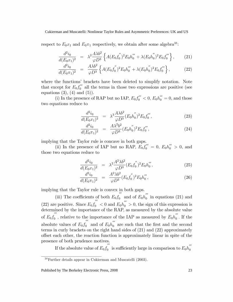
respect to E0x1 and E0�1 respectively, we obtain after some algebra38:

d2i0d(E0x1)2

= �2A�b2

'D3

nA(E0f

00

0 )2E0h

000

0 + �(E0h00

0 )2E0f

000

0

o; (21)

d2i0d(E0�1)2

=A�b2

'D3

nA(E0f

00

0 )2E0h

000

0 + �(E0h00

0 )2E0f

000

0

o; (22)

where the functions�brackets have been deleted to simplify notation. Notethat except for E0f

0000 all the terms in those two expressions are positive (see

equations (3), (4) and (5)).(i) In the presence of RAP but no IAP, E0f

0000 < 0; E0h

0000 = 0, and those

two equations reduce to

d2i0d(E0x1)2

= �3A�b2

'D3(E0h

00

0 )2E0f

000

0 ; (23)

d2i0d(E0�1)2

=A�2b2

'D3(E0h

00

0 )2E0f

000

0 ; (24)

implying that the Taylor rule is concave in both gaps.(ii) In the presence of IAP but no RAP, E0f

0000 = 0; E0h

0000 > 0, and

those two equations reduce to

d2i0d(E0x1)2

= �2A2�b2

'D3(E0f

00

0 )2E0h

000

0 ; (25)

d2i0d(E0�1)2

=A2�b2

'D3(E0f

00

0 )2E0h

000

0 ; (26)

implying that the Taylor rule is convex in both gaps.

(iii) The coe¢ cients of both E0f000

0 and of E0h000

0 in equations (21) and

(22) are positive. Since E0f000

0 < 0 and E0h000

0 > 0; the sign of this expression isdetermined by the importance of the RAP, as measured by the absolute value

of E0f000

0 ; relative to the importance of the IAP as measured by E0h000

0 : If the

absolute values of E0f000

0 and of E0h000

0 are such that the �rst and the secondterms in curly brackets on the right hand sides of (21) and (22) approximatelyo¤set each other, the reaction function is approximately linear in spite of thepresence of both prudence motives.

If the absolute value of E0f000

0 is su¢ ciently large in comparison to E0h000

0

38Further details appear in Cukierman and Muscatelli (2003).

23



(the RAP dominates the IAP), the right-hand sides of equations (21) and (22)are negative and the Taylor rule is concave in both gaps. If the converse holds,the right-hand sides of equations (21) and (22) are positive and the Taylor ruleis convex in both gaps.

(iv) If the CB is a strict in�ation targeter, A = 0, and the expressions inequations (21) and (22) are equal to zero, implying that the reaction functionis linear. QED

5.2 An equivalence relation between the sign of �2 andthe curvature of the HTSTR with respect to ex-pected in�ation

This part of the Appendix states and proves a condition on rates of in�ationwhich establishes a clear-cut equivalence between the sign of �2 and the sec-ond derivative of the estimated hyperbolic tangent regressions with respect toexpected in�ation.

Proposition 2: For in�ation gaps that are not too large in absolutevalue, the estimated hyperbolic tangent regressions are convex or concave inexpected in�ation depending on whether �2 is positive or negative

Proof: Di¤erentiating (20) with respect to �t;1:

@2i

@�2t;1= �2

h2 tanh

0[ (�t;1 � ��)] + (�t;1 � ��) tanh

00[ (�t;1 � ��)]

i; (27)

where tanh0[:] and tanh

00[:] are the �rst and second derivatives of the hyper-

bolic tangent with respect to its argument. Since > 0 the sign of @2i@�2t;1

is the

same as that of �2 if and only if the expression in brackets on the right-handside of (27) is positive. Rearranging, using the explicit formula for the hyper-

bolic tangent in (18) to calculate tanh0[:] and tanh

00[:] and the fact that it is

convex (concave) when the in�ation gap is negative (positive), the expressionin brackets on the right-hand side of (27) is positive if and only if

�t;1 � �� >1

1

tanh [ (�t;1 � ��)]; �t;1 � �� < 0; (28)

�t;1 � �� <1

1

tanh [ (�t;1 � ��)]; �t;1 � �� > 0: (29)

24



Since = 0:2 in all the HTSTR those conditions reduce to

�t;1 � �� >5

tanh [0:2(�t;1 � ��)]; �t;1 � �� < 0; (30)

�t;1 � �� <5

tanh [0:2(�t;1 � ��)]; �t;1 � �� > 0: (31)

The right-hand side of (30) is negative and that of (31) is positive. For ratesof in�ation (or de�ation) su¢ ciently close to any positive in�ation target,�� > 0; the conditions in those equations are satis�ed, since in such a casethe right-hand side of (30) is a very large negative number and the right-handside of (31) is a very large positive number. As the distance between �t;1 andthe target grows in either direction, the margin by which those conditions aresatis�ed shrinks monotonically until the inequalities in equations (30) and (31)are reversed. But as long as the in�ation gap is not too large in absolute value,the expression in square brackets on the right-hand side of (27) is positive andthe sign of @2i

@�2t;1is the same as that of �2, so that the HTSTR are convex or

concave depending on whether �2 is positive or negative. QEDThe critical in�ation rates beyond which the term in brackets on the

right hand side of (27) becomes negative are determined implicitly from

�cL = �� +5

tanh [0:2(�cL � ��)]; �cL < ��;

�cH = �� +5

tanh [0:2(�cH � ��)]; �cH > ��: (32)

Thus, as long as �cL < �t;1 < �cH the result in proposition 2 applies,and the response of the interest rate to expected in�ation is convex or concavedepending on whether �2 is positive or negative.

39 Using the values of thein�ation targets from Table 1, these ranges, for the 1979-90 and 1992-05 sub-samples in the UK, are given by 1:5 < �t;1 < 13:5 and �3:5 < �t;1 < 8:5respectively. Except for the �rst year of the �rst subperiod, these conditionsare always satis�ed in the UK. In the case of the US, the relevant ranges forthe Martin and Greenspan periods are given respectively by �4:7 < �t;1 <7:3 and �3:1 < �t;1 < 8:9. These conditions are always satis�ed. For theBurns/Miller period the relevant range is �2:8 < �t;1 < 9:2: Excluding fourquarters following the �rst oil shock and four quarters following the second oil

39Equations (32) imply (since tanh is symmetric around zero) that �cL � �� = �( �cH ��) = 6:0:

25



shock, in�ation is always in this range during the Burns/Miller era.

5.3 An equivalence relation between the sign of 2 andthe curvature of the HTSTR with respect to theexpected output gap

Using arguments similar to those used in the proof of proposition 2 one canestablish the following proposition:

Proposition 3: For output gaps that are smaller in absolute valuethan a critical gap, j xc j; the estimated hyperbolic tangent regressions areconvex or concave in the expected output depending on whether 2 is positiveor negative. For = 0:2; the critical value of the output gap is implicitlydetermined from

j xc j�5

tanh [ j xc j]:

For = 0:2, j xc j= 5:998. Practically all the values of the output gaps inour samples are below this critical value in absolute terms. For the UK thiscondition is always satis�ed. For the US, except for �ve observations (the datapoint 1966-1 and the period 1982-1-to 1983-1), again this condition holds.

5.4 Data sources and de�nitions

UK:Y �real output �Main Economic Indicators �OECD, Quarterly series:

March 2006Series [GBR.CMPGDP.VIXOBSA]YBAR �OECD�s Estimate of Potential GDP.x �percentage deviations of Y from YBAR.i �Bank of England intervention rate �end quarterSource: Bank of England - compound series using BoE repo rate, and

eligible bills discount rateRPIX �UK Quarterly Index of Retail Prices � All items excluding

mortgage interest paymentsSource: O¢ ce for National Statistics (ONS)� �annualized quarterly percentage change in the RPIX.

USA:Y �real output - Main Economic Indicators �OECD, Quarterly series:

March 2006

26



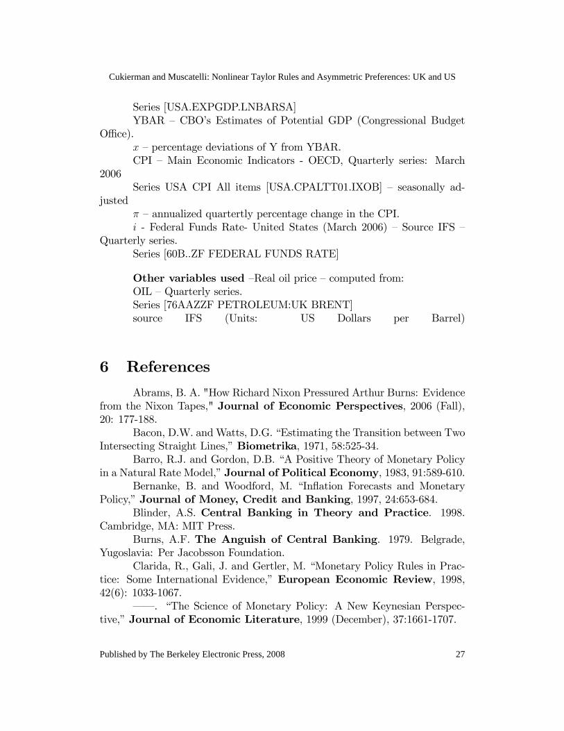
Series [USA.EXPGDP.LNBARSA]YBAR �CBO�s Estimates of Potential GDP (Congressional Budget

O¢ ce).x �percentage deviations of Y from YBAR.CPI �Main Economic Indicators - OECD, Quarterly series: March

2006Series USA CPI All items [USA.CPALTT01.IXOB] � seasonally ad-

justed� �annualized quartertly percentage change in the CPI.i - Federal Funds Rate- United States (March 2006) �Source IFS �

Quarterly series.Series [60B..ZF FEDERAL FUNDS RATE]

Other variables used �Real oil price �computed from:OIL �Quarterly series.Series [76AAZZF PETROLEUM:UK BRENT]source IFS (Units: US Dollars per Barrel)

6 References

Abrams, B. A. "How Richard Nixon Pressured Arthur Burns: Evidencefrom the Nixon Tapes," Journal of Economic Perspectives, 2006 (Fall),20: 177-188.

Bacon, D.W. andWatts, D.G. �Estimating the Transition between TwoIntersecting Straight Lines,�Biometrika, 1971, 58:525-34.

Barro, R.J. and Gordon, D.B. �A Positive Theory of Monetary Policyin a Natural Rate Model,�Journal of Political Economy, 1983, 91:589-610.

Bernanke, B. and Woodford, M. �In�ation Forecasts and MonetaryPolicy,�Journal of Money, Credit and Banking, 1997, 24:653-684.

Blinder, A.S. Central Banking in Theory and Practice. 1998.Cambridge, MA: MIT Press.

Burns, A.F. The Anguish of Central Banking. 1979. Belgrade,Yugoslavia: Per Jacobsson Foundation.

Clarida, R., Gali, J. and Gertler, M. �Monetary Policy Rules in Prac-tice: Some International Evidence,�European Economic Review, 1998,42(6): 1033-1067.

� � . �The Science of Monetary Policy: A New Keynesian Perspec-tive,�Journal of Economic Literature, 1999 (December), 37:1661-1707.

27



� � . �Monetary Policy Rules and Macroeconomic Stability: Evidenceand Some Theory,�Quarterly Journal of Economics, 2000 (February),113:147-180.

Cukierman, A. �Why Does the Fed Smooth Interest Rates?�in M. Be-longia (ed.), Monetary Policy on the Fed�s 75th Anniversary �Proceedingsof the 14th Annual Economic Policy Conference of the Federal Re-serve Bank of St. Louis. 1990. Kluwer Academic Publishers, pp. 111-147.

� � . Central Bank Strategy, Credibility and Independence:Theory and Evidence. 1992. Cambridge, MA: MIT Press.

� � . �The In�ation Bias Result Revisited,�April 2000. Manuscript,Tel-Aviv University. Available on the Internet at:

www.tau.ac.il/~alexcuk/pdf/infbias1.pdf� � . �Are Contemporary Central Banks Transparent about Economic

Models and Objectives andWhat Di¤erence Does It Make?�Federal ReserveBank of St. Louis Review, 2002 (July-August), 84(4):15-45.

Cukierman, A. and Gerlach, S. �The In�ation Bias Result Revisited:Theory and Some International Evidence,�The Manchester School, 2003(September), 71(5):541-565.

Cukierman, A. and Muscatelli, A. �Do Central Banks Have Precaution-ary Demands for Expansions and for Price Stability? �A New Keynesian Ap-proach.�2003. Available on the web at www.tau.ac.il/~alexcuk/pdf/cukierman-muscatelli-03a.pdf

Dolado, J., Pedrero, R.M.D. and Ruge-Murcia, F. �Nonlinear Mone-tary Policy Rules: Some New Evidence for the US,�Studies in NonlinearDynamics and Econometrics, 2004, 8, issue 3.

Geraats, P. �In�ation and Its Variation: An Alternative Explanation,�2006. Manuscript (revision of CIDER Working Paper C99-105, Departmentof Economics, University of California, Berkeley, July 1999).

Granger, C.W.J. and Terasvirta, T. Modelling Non-Linear Eco-nomic Relationships. 1993. Oxford: Oxford University Press.

Hansen, L.P. �Large Sample Properties of Generalized Method of Mo-ments Estimators,�Econometrica, 1982, 50:1029-54.

Kimball, M.S. �Precautionary Saving in the Small and in the Large,Econometrica, 1990 (January), 58:53-73.

Kydland, F.E. and Prescott, E.C. �Rules Rather than Discretion: TheInconsistency of Optimal Plans,� Journal of Political Economy, 1977,85:473-92.

Lindsey, D., Orphanides, A. and Rasche, R. �The Reform of October1979: How It Happened and Why,�Federal Reserve Bank of St. LouisReview, 2005 (March-April), 82, 2(2):187-235.

28



Meltzer A. H.A History of the Federal Reserve, Volume 2. 2008.Chicago and London: University of Chicago Press, Forthcoming.

Mishkin, F. and Posen, A. �In�ation Targeting: Lessons from FourCountries,�Federal Reserve Bank of NY Economic Policy Review,1997 (August), 3(3):9-110.

Muscatelli, V.A., Tirelli, P. and Trecroci, C. �Does Institutional ChangeReally Matter? In�ation Targets, Central Bank Reform and Interest RatePolicy in the OECD Countries,�The Manchester School, Special Issue onIn�ation Targeting, 2002, 70(4):487-527.

Muscatelli, V.A. and Trecroci, C. �Central Bank Goals, InstitutionalChange and Monetary Policy: Evidence from the US and UK,�in L. Mahadevaand P. Sinclair (eds.), Monetary Transmissions in Diverse Economies.2002. Cambridge and London: Cambridge University Press and Bank of Eng-land.

Nobay, R. and Peel, D. �Optimal Monetary Policy in a Model of Asym-metric Central Bank Preferences,�1998. Manuscript, London School of Eco-nomics.

Ruge-Murcia, F.J. �De�ation and Optimal Monetary Policy,�October2000. Manuscript, University of Montreal.

� � . �Does the Barro-Gordon Model Explain the Behavior of US In-�ation? A Reexamination of the Empirical Evidence,�Journal of MonetaryEconomics, 2003, 50:1375-1390.

Seber, G.A.F. and Wild, C.J. Non-Linear Regression. 1989. NewYork: Wiley.

Surico, P. �The Fed�s Monetary Policy Rule and US In�ation: TheCase of Asymmetric Preferences,� Journal of Economic Dynamics andControl, 2007, 31:305-324.

Sussman, N. �Monetary Policy in Israel, 1986-2000: Estimating theCentral Bank�s Reaction Function,�in N. Liviatan and H. Barkai (eds.), TheBank of Israel: Volume II, Selected Topics in Israel�s Monetary Pol-icy. 2007. Oxford, New York: Oxford University Press.

Svensson, L.E.O. �Open-Economy In�ation Targeting,� Journal ofInternational Economics, 2000, 50:155-183.

Wood J. H. A History of Central Banking in Great Britain andthe United States. 2005. Cambridge and New York: Cambridge UniversityPress.

29



Documents

The B.E. Journal of Macroeconomics - TAUalexcuk/pdf/Cukierman-Muscatelli_B.E.J.M._Issue_1... · The B.E. Journal of Macroeconomics Contributions Volume 8, Issue 1 2008 Article 7 Nonlinear