NBER WORKING PAPER SERIES

THE BENEFITS OF COLLEGE ATHLETIC SUCCESS:AN APPLICATION OF THE PROPENSITY SCORE DESIGN WITH INSTRUMENTAL VARIABLES

Michael L. Anderson

Working Paper 18196http://www.nber.org/papers/w18196

NATIONAL BUREAU OF ECONOMIC RESEARCH1050 Massachusetts Avenue

Cambridge, MA 02138June 2012

I thank David Card and Jeremy Magruder for insightful comments and am grateful to Tammie Vuand Yammy Kung for excellent research assistance. Funding for this project was provided by the CaliforniaAgricultural Experiment Station. The views expressed herein are those of the author and do not necessarilyreflect the views of the National Bureau of Economic Research.

NBER working papers are circulated for discussion and comment purposes. They have not been peer-reviewed or been subject to the review by the NBER Board of Directors that accompanies officialNBER publications.

© 2012 by Michael L. Anderson. All rights reserved. Short sections of text, not to exceed two paragraphs,may be quoted without explicit permission provided that full credit, including © notice, is given tothe source.

The Benefits of College Athletic Success: An Application of the Propensity Score Designwith Instrumental VariablesMichael L. AndersonNBER Working Paper No. 18196June 2012JEL No. C23,C26,I20,I23,J24

ABSTRACT

Spending on big-time college athletics is often justified on the grounds that athletic success attractsstudents and raises donations. Testing this claim has proven difficult because success is not randomlyassigned. We exploit data on bookmaker spreads to estimate the probability of winning each gamefor college football teams. We then condition on these probabilities using a propensity score designto estimate the effects of winning on donations, applications, and enrollment. The resulting estimatesrepresent causal effects under the assumption that, conditional on bookmaker spreads, winning is uncorrelatedwith potential outcomes. Two complications arise in our design. First, team wins evolve dynamicallythroughout the season. Second, winning a game early in the season reveals that a team is better thananticipated and thus increases expected season wins by more than one-for-one. We address these complicationsby combining an instrumental variables-type estimator with the propensity score design. We find thatwinning reduces acceptance rates and increases donations, applications, academic reputation, in-stateenrollment, and incoming SAT scores.

Michael L. AndersonDepartment of Agricultural and Resource Economics207 Giannini Hall, MC 3310University of California, BerkeleyBerkeley, CA 94720and NBERmlanderson@berkeley.edu

1 Introduction

College athletic spending at National Collegiate Athletic Association (NCAA) Division I

schools exceeded $7.9 billion in 2010 (Fulks 2011). This scale of expenditures is interna-

tionally unique and is partly justified on the basis that big-time athletic success, particularly

in football and basketball, attracts students and generates donations. An extensive litera-

ture examines these claims but reaches inconsistent conclusions. A series of papers find

positive effects of big-time athletic success on applications and contributions (Brooker and

Klastorin 1981; Sigelman and Bookheimer 1983; Grimes and Chressanthis 1994; Murphy

and Trandel 1994; Tucker 2004; Humphreys and Mondello 2007; Pope and Pope 2009),

but a number of other studies find no impact of big-time athletic success on either measure

(Sigelman and Carter 1979; Baade and Sundberg 1996; Turner et al. 2001; Meer and Rosen

2009; Orszag and Israel 2009). A central issue confronting all studies is the non-random

assignment of athletic success. Schools with skilled administrators may attract donations,

applicants, and coaching talent (selection bias), and surges in donations or applications

may have a direct impact on athletic success (reverse causality). It is thus challenging to

estimate causal effects of athletic success using observational data.

This article estimates the causal effects of college football success using a propensity

score design. Propensity score methods are difficult to apply because researchers seldom

observe all of the important determinants of treatment assignment. Treatment assignment

is thus rarely ignorable given the data at the researcher’s disposal (Rosenbaum and Ru-

bin 1983; Dehejia and Wahba 1999). We overcome this challenge by exploiting data on

bookmaker spreads (i.e., the expected score differential between the two teams) to estimate

the probability of winning each game for NCAA “Division I-A” football teams. We then

condition on these probabilities to estimate the effect of football success on donations and

applications. If potential outcomes are independent of winning games after conditioning

on bookmaker expectations, then our estimates represent causal effects.

We face two complications when estimating these effects. First, the treatment – team

wins – evolves dynamically throughout the season, and the propensity score for each win

depends on the outcomes of previous games. We address this issue by independently esti-

2

mating the effect of wins in each week of the season. However, this introduces the second

complication: a win early in the season is associated with a greater than one-for-one in-

crease in total season wins because the winning team has (on average) revealed itself to be

better than expected. We address this issue by combining an instrumental variables-type

estimator with the propensity score estimator.

Applying this framework we find robust evidence that football success increases athletic

donations, increases the number of applicants, lowers a school’s acceptance rate, increases

enrollment of in-state students, increases the average SAT score of incoming classes, and

enhances a school’s academic reputation. The estimates are up to twice as large as com-

parable estimates from the previous literature. There is less evidence that football success

affects donations outside of athletic programs or enrollment of out-of-state students. The

effects appear concentrated among teams in the six elite conferences classified as “Bowl

Championship Series” (BCS) conferences, with less evidence of effects for teams in other

conferences.

The paper is organized as follows. Section 2 describes the data, and Section 3 summa-

rizes the cross-sectional and longitudinal relationships between football success, donations,

and student body measures. Section 4 discusses the propensity score framework and esti-

mation strategy. Section 5 presents estimates of the causal relationships between football

success, donations, and student body measures. Section 6 concludes.

2 Data

Approximately 350 schools participate in NCAA Division I sports (the highest division of

intercollegiate athletics). Of these schools, 120 field football teams in the Football Bowl

Subdivision (FBS, formerly known as “Division I-A”). Teams in this subdivision play 10

to 13 games per season and are potentially eligible for post-season bowl games. Games

between teams in this subdivision are high-profile events that are widely televised. We

gathered data on games played by all FBS teams from 1986 to 2009 from the website

Covers.com. Data include information on the game’s date, the opponent, the score of each

team, and the expected score differential between the two teams (known as the spread).

3

We combined these data with data on alumni donations, university academic reputa-

tions, applicants, acceptance rates, enrollment figures, and average SAT scores. Donations

data come from the Voluntary Support of Education survey (VSE), acceptance rate and

academic reputation data come from a survey of college administrators and high school

counselors conducted annually by US News and World Report, and application, enrollment,

and SAT data come from the Integrated Postsecondary Education Data System (IPEDS).

Reporting dates for these measures range from 1986 to 2008.

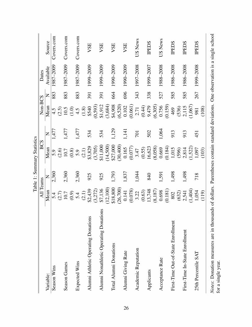
The first column of Table 1 presents summary statistics for key variables. Each ob-

servation represents a single season for a single team. Actual season wins and expected

season wins are both 5.4 games per season (out of an average of 10.7 games played per

season). We exclude post-season games (bowl games) when calculating wins as participa-

tion in these games is endogenously determined by regular season wins. Alumni donations

to athletic programs average $2.4 million per year, and total alumni donations (including

both operating and capital support) average $18.8 million per year. The average school

receives 13,748 applicants every year and accepts 70% of them. A typical incoming class

contains 3,343 students and has a 25th percentile SAT score of 1,054 (IPEDS reports 25th

and 75th percentile SAT scores; using the 75th percentile instead of the 25th percentile

does not affect our conclusions).

The next two sets of columns in Table 1 present summary statistics for BCS and non-

BCS conferences respectively. The six BCS conferences are the ACC, Big East, SEC, Big

Ten, Big Twelve, and Pac-10 (now Pac-12). Winners of these conferences are automat-

ically eligible for one of ten slots in the five prestigious BCS bowl games, and through

2012 only three non-BCS conference teams had ever played in a BCS bowl game. Teams

in BCS conferences have more wins (note that inter-conference play is common), more

alumni donations, better academic reputations, lower acceptance rates, and more appli-

cants and enrolled students than teams in non-BCS conferences. Since BCS conference

football teams have higher profiles, we expect that team success may have a larger impact

for these schools (particularly for alumni donations), and we estimate results separately for

BCS conferences.

4

3 Cross-Sectional and Longitudinal Results

3.1 Cross-sectional Results

We first estimate the cross-sectional relationship between lagged win percentage, alumni

donations, and class characteristics. We estimate linear regressions of the form

yit+1 = β0 + β1season winsit + β2season gamesit + φt+1 + εit+1 (1)

where yit+1 represents an outcome for school i in year t + 1 (e.g., alumni donations, ap-

plicants, or acceptance rate), season winsit represents school i’s football wins in year t,

season gamesit represents school i’s football games played in year t, and φt+1 represents

a year fixed effect that controls for aggregate time trends. The coefficient of interest is β1.

We lag the win measure by one year because the college football season runs from Septem-

ber to December, so the full effects of a winning season on donations or applications are

unlikely to materialize until the following year.

The first set of columns in Table 2 reports results from estimating equation (1). One ex-

tra win is associated with a $340,400 increase in alumni athletic donations and a $960,100

increase in total alumni donations. Out-of-state and in-state enrollment increase by 34 and

91 students respectively. However, there is no significant relationship between wins and

non-athletic operating donations, the average donation rate, academic reputation, applica-

tions, the acceptance rate, or the 25th percentile SAT score.

The large number of hypothesis tests raises the issue of multiple hypothesis testing –

throughout the paper we test for effects on 10 different outcomes using multiple specifica-

tions and two subgroups (BCS and non-BCS schools). We address this issue by reporting

“q-values” that control the False Discovery Rate (FDR) across all tables, along with stan-

dard per-comparison p-values. The False Discovery Rate is the proportion of rejections

that are false discoveries (type I errors). Controlling FDR at 0.1, for example, implies that

less than 10% of rejections will represent false discoveries. To calculate FDR q-values we

use the “sharpened” FDR control algorithm from Benjamini et al. (2006), implemented in

Anderson (2008). In most cases statistical significance remains even after controlling FDR.

5

3.2 Longitudinal Results

It is unlikely that the cross-sectional estimates in Table 2 represent causal effects; some

unobserved factors that affect donations or applications are probably correlated with long-

term athletic success. To remove unobserved factors that vary across schools but are fixed

over time, we estimate linear regressions of the form

∆yit+1 = β0 + β1∆season winsit + β2∆season gamesit + φt+1 + εit+1 (2)

where

∆yit+1 = yit+1 − yit−1

∆season winsit = season winsit − season winsit−2

∆season gamesit = season gamesit − season gamesit−2

Other variables are as defined in equation (1), and the coefficient of interest is again β1.

We difference over two years rather than one year because season winsit may affect yit,

so estimating a regression using one-year differences may attenuate our estimates of β1.

Indeed, differencing over one year rather than two years generates estimates that are 46%

smaller in magnitude on average.1

The second set of columns in Table 2 reports results from estimating equation (2). A

one win increase is associated with a $74,000 increase in alumni athletic donations but

no statistically significant increases in total alumni donations or the alumni giving rate.

Academic reputation increases by 0.002 points (0.003 standard deviations). Applications

increase by 104 per year, acceptance rates drop 0.2 percentage points, and in-state enroll-

ment increases by 17 students. There is no significant relationship between increases in

wins and out-of-state enrollment or the 25th percentile SAT score.

Two patterns appear when comparing the cross-sectional and longitudinal estimates.

First, the longitudinal estimates are much more precise, with standard errors that are ap-

1The divergence between the two-year differences results and the one-year differences results is largestfor the acceptance rate estimate, which falls by 71%, and smallest for the SAT score estimate, which falls by4%

6

proximately 3 to 15 times smaller. This is because much of the unexplained variation in

yit occurs across schools rather than within schools, and the differencing transformation in

equation (2) removes most of the cross-school variation in yit. Second, with the exception

of acceptance rates, the longitudinal estimates are all smaller in magnitude than their cross-

sectional counterparts. In several cases (alumni athletic donations, out-of-state enrollment,

and in-state enrollment) it is possible to reject the hypothesis that the cross-sectional and

longitudinal estimates converge to the same value. The divergence in the two sets of es-

timates suggests the presence of selection bias or reverse causality, though it could also

indicate persistence in effects (i.e., several winning seasons may have a larger impact than

a single winning season).

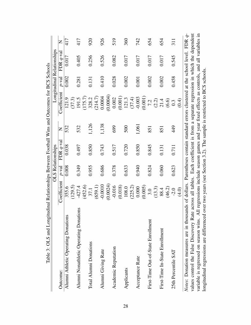
3.3 BCS Results

Teams in BCS conferences have higher profiles and thus may experience greater impacts

from football success. Table 3 reports cross-sectional and longitudinal results for BCS

teams. The first set of columns estimates equation (1). There is a significant relationship

between wins and alumni athletic donations, but no other coefficients are significant at

the p = 0.05 level. In most cases the cross-sectional estimates from the BCS sample are

smaller than the cross-sectional estimates from the pooled sample. Estimates from the non-

BCS sample are smaller still (see Appendix Table A1). Since conditioning on BCS status

is equivalent to flexibly controlling for BCS status, this pattern suggests that unobserved

differences between BCS and non-BCS schools may affect the pooled cross-sectional esti-

mates.

The second set of columns in Table 3 estimates equation (2). Significant longitudinal

relationships arise between wins and alumni athletic donations, academic reputation, appli-

cations, acceptance rates, and in-state and out-of-state enrollment. Longitudinal estimates

from the BCS sample are of the same sign and typically larger magnitude when compared

to longitudinal estimates from the pooled sample. This suggests that effects may be concen-

trated among BCS schools. Indeed, longitudinal estimates from the non-BCS sample are

generally smaller in magnitude, and all but one are statistically insignificant (see Appendix

7

Table A1).

4 The Propensity Score Design

4.1 Theoretical Framework

Longitudinal estimates control for unobserved factors that differ across schools but are

constant over time. Nevertheless, they should be interpreted with caution (LaLonde 1986);

changes in donations or admissions could be related to changes in wins through reverse

causality, and trends in other factors (e.g., coaching talent) might be related to both sets of

variables. One way to improve the research design is to condition on observable factors

that determine football wins. However, two problems arise in this context. First, we do not

have data on a wide range of factors that plausibly determine whether a team wins. Second,

even if such data were available, conditioning on a large number of factors introduces

dimensionality problems and makes estimation via matching or subclassification difficult.

In cases with binary treatments, conditioning on the propensity score – the probabil-

ity of treatment given the observable characteristics – is equivalent to conditioning on the

observables themselves (Rosenbaum and Rubin 1983; Dehejia and Wahba 1999). Condi-

tioning on the propensity score, or the probability of a win, is attractive in this case for

two reasons. First, it is readily estimable using bookmaker spreads. Second, it is of low

dimension.

However, the treatment season winsit is not binary but can instead realize integer

values from 0 to 12. Furthermore, it is dynamically determined – each game occurs at

a different point in the season. Recent research has extended propensity score methods

to cases with categorical and continuous treatments (Hirano and Imbens 2004; Imai and

van Dyk 2004). Since the distribution of a bounded random variable is defined by its mo-

ments, we could in principle calculate the conditional expectation, variance, and skewness

of season winsit and condition on these quantities. In practice, however, we cannot cal-

culate these conditional moments because bookmaker spreads are updated throughout the

season. Importantly, bookmaker spreads in week s are a function of the team’s performance

8

in weeks 1 through s − 1. Bookmaker spreads are thus endogenously determined by the

treatment itself.

To overcome this problem we separately estimate the effect of winning for each week

of the season. This ensures that the set of conditioning variables is always predetermined

with respect to the treatment. Formally, let the treatment Wist equal one if school i wins in

week s of year t and zero otherwise. The 1 × S row vector wit contains the outcome of

each game for the entire season, with the sth column containing the outcome for week s.

The potential outcome Yit+1(wi1t, ..., wiSt) is the value of the outcome for school i in year

t+ 1 as a function of wit. Conditional on wins and losses in other weeks, the causal effect

of a win in week s for school i in year t is βist = Yit+1(wi1t, ..., wis−1t, 1, wis+1t, ..., wiSt)−

Yit+1(wi1t, ..., wis−1t, 0, wis+1t, ..., wiSt). For notational convenience we write Yist(1) =

Yit+1(wi1t, ..., wis−1t, 1, wis+1t, ..., wiSt) and Yist(0) = Yit+1(wi1t, ..., wis−1t, 0, wis+1t, ..., wiSt).

While there are many potential outcomes for any combination of i, s, and t, we can

only observe Yit+1(wit), where wit is the realized series of wins and losses for school i in

year t. If wins were randomly assigned, then Yit+1(wit) would be independent of Wist for

all values of wit, and we could estimate E[Yist(1)] and E[Yist(0)] using the sample analogs

of E[Yit+1|Wist = 1] and E[Yit+1|Wist = 0]. However, in all likelihood the potential

outcomes Yit+1(wit) are correlated with Wist.

To estimate the causal effects of football wins we rely on two assumptions. First, we

make the standard ignorability assumption:

Assumption 1 Strong Ignorability of Treatment Assignment (Rosenbaum and Rubin 1983):

Wist ⊥ {Yit+1(wit) : wit ∈ W} | Xist. Furthermore, 0 < P (Wist = 1|Xist) < 1 ∀ Xist ∈

X .

The ignorability assumption is crucial. It implies that, conditional on the observables

Xist, Wist is independent of the potential outcomes Yit+1(wit). The ignorability assump-

tion has two unique features in our study. First, Xist represents the set of covariates ob-

served by bookmakers in week s of year t rather than set of covariates available to us the

researchers. Second, there is a strong economic reason to believe that Xist contains all

of the important observables. If there were an observable characteristic x∗ist that predicted

9

Wist and were not included in Xist, then professional bettors could use x∗ist to form supe-

rior predictions of P (Wist = 1) than those formed by the bookmakers. This discrepancy

would represent an arbitrage opportunity, and over time bookmakers would go bankrupt

if they did not condition their spreads on x∗ist. Thus, unlike in many data sets, we have a

compelling reason to believe that the ignorability assumption holds. Studies of betting mar-

kets support this conjecture in that it has proven difficult to build models that outperform

bookmakers’ spreads by an economically meaningful margin (Glickman and Stern 1998;

Levitt 2004; Stern 2008). Of course, it is theoretically possible that some characteristic

that is unobservable to everyone and affects the probability of winning is correlated with

the potential outcomes. As a robustness check, we reestimate the effects later in the season

when team quality becomes well known, and we find similar results (see Section 5.2).

Proposition 1 Let p(Xist) = P (Wist = 1 | Xist). Under strong ignorability, Wist ⊥

{Yit+1(wit) : wit ∈ W} | p(Xist).

Proof : See Appendix A.

Corollary: Under strong ignorability, if Cov(Yit+1,Wist | p(Xist)) 6= 0, then Wist must

have a causal effect on Yit+1 for some values of i, s, t.

Proof : Suppose that Wist has no casual effect on Yit+1 for any values of i, s, t. Then

Yit+1(wit) = Yit+1 for any wit ∈ W . Thus, by Proposition 1, Wist ⊥ Yit+1 | p(Xist).

Proposition 1 implies that we can test for a causal effect of Wist on Yit+1 by condi-

tioning on p(Xist) and estimating a regression of Yit+1 on Wist. A significant regression

coefficient in this case allows us to reject the sharp null hypothesis of no effect, and we

use this proposition to estimate p-values in Tables 4–7. These tests are similar in spirit to

propensity score based tests in recent research by Angrist and Kuersteiner on the effects of

monetary policy shocks. However, to estimate the magnitude of the causal effect we make

two additional assumptions.

Assumption 2 Ignorability of Future Treatment Assignments: (Wis+1t, ...,WiSt) ⊥ {Yit+1(wit) :

wit ∈ W} | Xist.

10

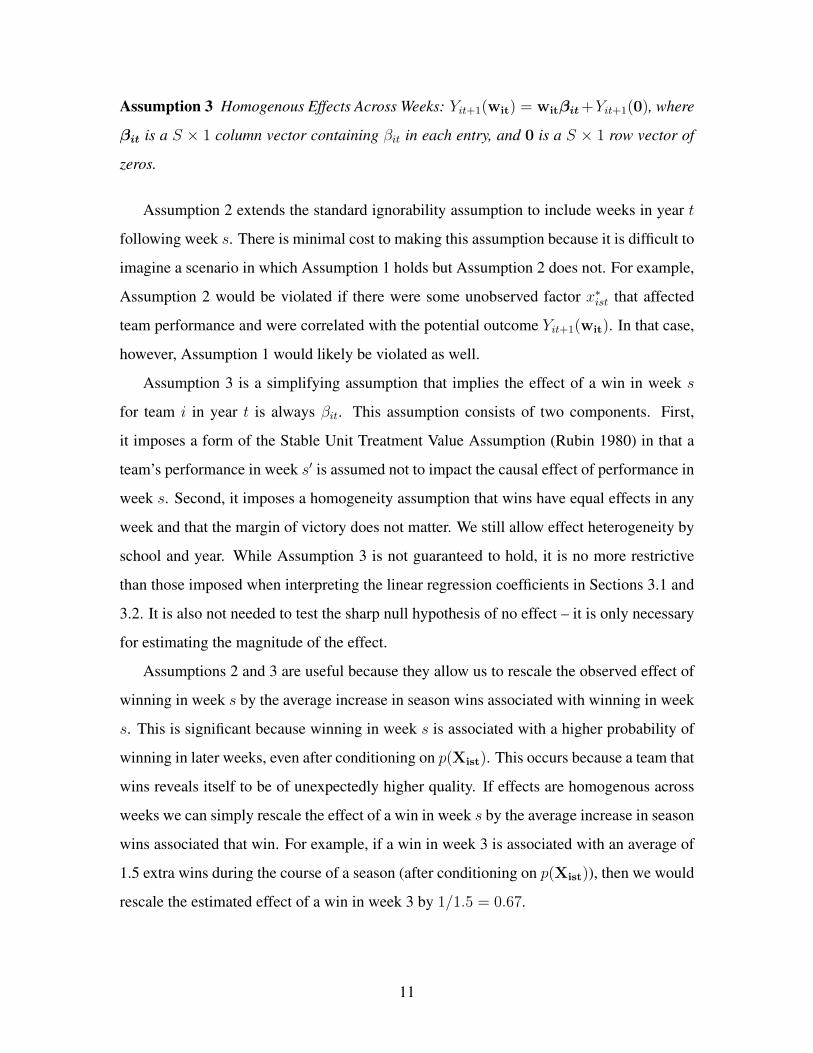
Assumption 3 Homogenous Effects Across Weeks: Yit+1(wit) = witβit +Yit+1(0), where

βit is a S × 1 column vector containing βit in each entry, and 0 is a S × 1 row vector of

zeros.

Assumption 2 extends the standard ignorability assumption to include weeks in year t

following week s. There is minimal cost to making this assumption because it is difficult to

imagine a scenario in which Assumption 1 holds but Assumption 2 does not. For example,

Assumption 2 would be violated if there were some unobserved factor x∗ist that affected

team performance and were correlated with the potential outcome Yit+1(wit). In that case,

however, Assumption 1 would likely be violated as well.

Assumption 3 is a simplifying assumption that implies the effect of a win in week s

for team i in year t is always βit. This assumption consists of two components. First,

it imposes a form of the Stable Unit Treatment Value Assumption (Rubin 1980) in that a

team’s performance in week s′ is assumed not to impact the causal effect of performance in

week s. Second, it imposes a homogeneity assumption that wins have equal effects in any

week and that the margin of victory does not matter. We still allow effect heterogeneity by

school and year. While Assumption 3 is not guaranteed to hold, it is no more restrictive

than those imposed when interpreting the linear regression coefficients in Sections 3.1 and

3.2. It is also not needed to test the sharp null hypothesis of no effect – it is only necessary

for estimating the magnitude of the effect.

Assumptions 2 and 3 are useful because they allow us to rescale the observed effect of

winning in week s by the average increase in season wins associated with winning in week

s. This is significant because winning in week s is associated with a higher probability of

winning in later weeks, even after conditioning on p(Xist). This occurs because a team that

wins reveals itself to be of unexpectedly higher quality. If effects are homogenous across

weeks we can simply rescale the effect of a win in week s by the average increase in season

wins associated that win. For example, if a win in week 3 is associated with an average of

1.5 extra wins during the course of a season (after conditioning on p(Xist)), then we would

rescale the estimated effect of a win in week 3 by 1/1.5 = 0.67.

11

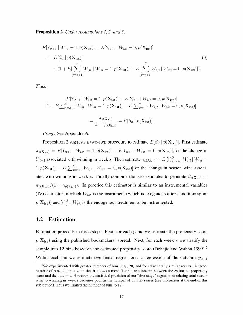
Proposition 2 Under Assumptions 1, 2, and 3,

E[Yit+1 |Wist = 1, p(Xist)]− E[Yit+1 |Wist = 0, p(Xist)]

= E[βit | p(Xist)] (3)

×(1 + E[S∑

j=s+1

Wijt |Wist = 1, p(Xist)]− E[S∑

j=s+1

Wijt |Wist = 0, p(Xist)]).

Thus,

E[Yit+1 |Wist = 1, p(Xist)]− E[Yit+1 |Wist = 0, p(Xist)]

1 + E[∑S

j=s+1Wijt |Wist = 1, p(Xist)]− E[∑S

j=s+1Wijt |Wist = 0, p(Xist)]

=πp(Xist)

1 + γp(Xist)

= E[βit | p(Xist)].

Proof : See Appendix A.

Proposition 2 suggests a two-step procedure to estimate E[βit | p(Xist)]. First estimate

πp(Xist) = E[Yit+1 | Wist = 1, p(Xist)] − E[Yit+1 | Wist = 0, p(Xist)], or the change in

Yit+1 associated with winning in week s. Then estimate γp(Xist) = E[∑S

j=s+1Wijt |Wist =

1, p(Xist)] − E[∑S

j=s+1Wijt | Wist = 0, p(Xist)] or the change in season wins associ-

ated with winning in week s. Finally combine the two estimates to generate βp(Xist) =

πp(Xist)/(1 + γp(Xist)). In practice this estimator is similar to an instrumental variables

(IV) estimator in which Wist is the instrument (which is exogenous after conditioning on

p(Xist)) and∑S

j=sWijt is the endogenous treatment to be instrumented.

4.2 Estimation

Estimation proceeds in three steps. First, for each game we estimate the propensity score

p(Xist) using the published bookmakers’ spread. Next, for each week s we stratify the

sample into 12 bins based on the estimated propensity score (Dehejia and Wahba 1999).2

Within each bin we estimate two linear regressions: a regression of the outcome yit+1

2We experimented with greater numbers of bins (e.g., 20) and found generally similar results. A largernumber of bins is attractive in that it allows a more flexible relationship between the estimated propensityscore and the outcome. However, the statistical precision of our “first stage” regressions relating total seasonwins to winning in week s becomes poor as the number of bins increases (see discussion at the end of thissubsection). Thus we limited the number of bins to 12.

12

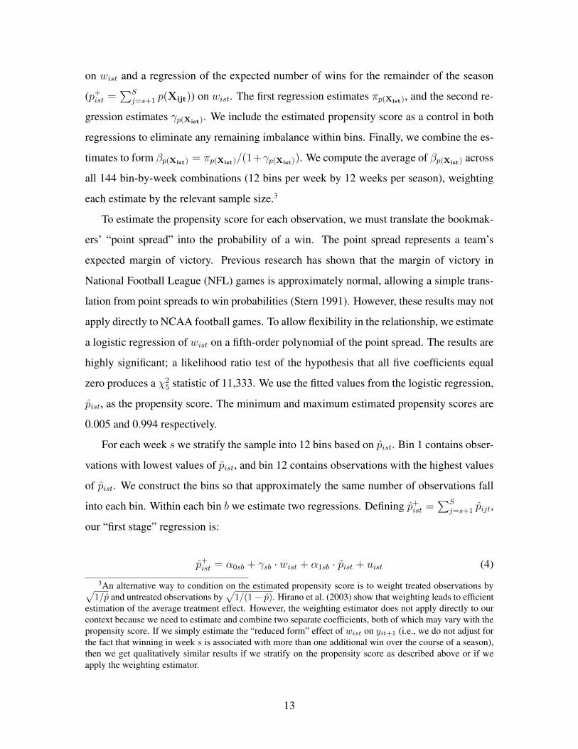
on wist and a regression of the expected number of wins for the remainder of the season

(p+ist =∑S

j=s+1 p(Xijt)) on wist. The first regression estimates πp(Xist), and the second re-

gression estimates γp(Xist). We include the estimated propensity score as a control in both

regressions to eliminate any remaining imbalance within bins. Finally, we combine the es-

timates to form βp(Xist) = πp(Xist)/(1+γp(Xist)). We compute the average of βp(Xist) across

all 144 bin-by-week combinations (12 bins per week by 12 weeks per season), weighting

each estimate by the relevant sample size.3

To estimate the propensity score for each observation, we must translate the bookmak-

ers’ “point spread” into the probability of a win. The point spread represents a team’s

expected margin of victory. Previous research has shown that the margin of victory in

National Football League (NFL) games is approximately normal, allowing a simple trans-

lation from point spreads to win probabilities (Stern 1991). However, these results may not

apply directly to NCAA football games. To allow flexibility in the relationship, we estimate

a logistic regression of wist on a fifth-order polynomial of the point spread. The results are

highly significant; a likelihood ratio test of the hypothesis that all five coefficients equal

zero produces a χ25 statistic of 11,333. We use the fitted values from the logistic regression,

p̂ist, as the propensity score. The minimum and maximum estimated propensity scores are

0.005 and 0.994 respectively.

For each week s we stratify the sample into 12 bins based on p̂ist. Bin 1 contains obser-

vations with lowest values of p̂ist, and bin 12 contains observations with the highest values

of p̂ist. We construct the bins so that approximately the same number of observations fall

into each bin. Within each bin b we estimate two regressions. Defining p̂+ist =∑S

j=s+1 p̂ijt,

our “first stage” regression is:

p̂+ist = α0sb + γsb · wist + α1sb · p̂ist + uist (4)

3An alternative way to condition on the estimated propensity score is to weight treated observations by√1/p̂ and untreated observations by

√1/(1− p̂). Hirano et al. (2003) show that weighting leads to efficient

estimation of the average treatment effect. However, the weighting estimator does not apply directly to ourcontext because we need to estimate and combine two separate coefficients, both of which may vary with thepropensity score. If we simply estimate the “reduced form” effect of wist on yit+1 (i.e., we do not adjust forthe fact that winning in week s is associated with more than one additional win over the course of a season),then we get qualitatively similar results if we stratify on the propensity score as described above or if weapply the weighting estimator.

13

The regression coefficient γ̂sb estimates the relationship between winning in week s

and winning during the remainder of the season, after conditioning on the propensity score

in week s. We can replace the dependent variable p+ist with the sum of observed wins,∑Sj=s+1wijt, without changing the results (though precision is reduced).

Our second regression is equivalent to a “reduced form” regression in an IV setting.

Our reduced form regression is:

yit+1 = δ0sb + πsb · wist + δ1sb · p̂ist + vist (5)

This regression estimates the relationship between winning in week s and the outcome

yit+1. Within each bin we then construct β̂sb = π̂sb/(1 + γ̂sb). After estimating equations

(4) and (5) for each bin b in each week s, we compute

β̂ =S∑

s=1

12∑b=1

β̂sb · rsb (6)

where the weights rsb sum to one and are proportional to the number of observations

(games) in bin b in week s.

We make two additional modifications to improve the procedure described above. First,

to ensure that the overlap assumption holds (i.e., 0 < p(Xist) < 1 ∀ Xist ∈ X ) we trim

the sample for each week s to eliminate all observations with propensity scores less than

the minimum score among winning observations for week s or greater than the maximum

score among losing observations for week s. To be conservative, we further restrict the

sample by dropping any observations with propensity scores less than 0.05 or greater than

0.95, and we eliminate any bins with less than two winning or two losing observations. Our

main conclusions are robust to relaxing these restrictions.4

Our second modification focuses on the “first stage”. Our raw first stage estimates of

γsb are relatively noisy since a typical bin contains less than 150 observations. If γ̂sb is near4For example, adding the restriction dropping any observations with propensity scores less than 0.05 or

greater than 0.95 does not change any of the estimated effects by more than 10%, except for the effect onSAT scores (which changes 13%). All of the restrictions combined do not change the statistical significanceof any of the effects, though they do impact the sizes of some estimates (in particular, the effects on alumnidonations, acceptance rates, and SAT scores change by 21%, 18%, and 30% respectively when all of therestrictions are added).

14

−1 in even a small number of cases, the confidence interval for β̂ becomes very wide, since

β̂sb = π̂sb/(1 + γ̂sb). This problem is well known in the instrumental variables literature

(Bound et al. 1995). To improve the precision of our first stage estimates, we assume that

the relationship betweenwist and∑S

j=s+1wijt is reasonably smooth in the propensity score.

For each week s we thus regress γ̂sb on a quadratic in the bin number (b and b2) and use the

fitted values from this regression as our estimates of γsb. This improves precision by using

information in bins near bin b to form the estimate of γsb. Alternatively, we could assume

that the first stage coefficient γsb does not vary with the covariates Xist and estimate a first

stage regression that pools observations across all 12 bins for week s. This is standard in

the instrumental variables literature (Angrist and Imbens 1995) and generates qualitatively

similar results.

5 Propensity Score Results

5.1 Baseline Results

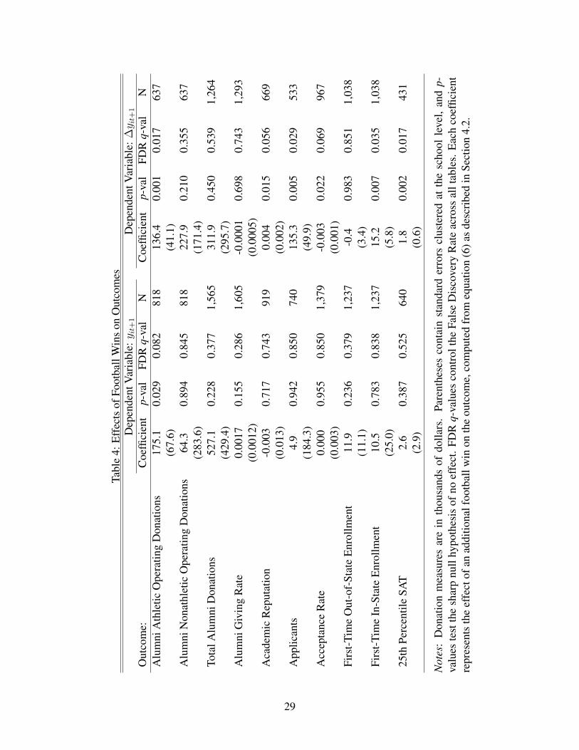
Table 4 reports the results of estimating equation (6) using all FBS (“Division I-A”) schools.

Each row reports the results for a different outcome. In the first set of columns we specify

the outcome in levels (yit+1), analogous to equation (1). In the second set of columns we

specify the outcome in two-year differences (∆yit+1), analogous to equation (2). Both

sets of estimates should be consistent under Assumptions 1–3, but estimates in the second

column are more precise because differencing removes much of the unexplained cross-

school variation in yit+1. Furthermore, differencing can help eliminate any bias that remains

after conditioning on the propensity score (Smith and Todd 2005). In this section we focus

on the differenced results (the second set of columns) because precision is limited in the

first set of columns.

Estimates from the propensity score design imply that an extra win increases alumni

athletic donations by $136,400. There are no statistically significant effects on non-athletic

donations, total donations, or the alumni giving rate, though we lack sufficient precision

to rule out economically significant effects. An extra win increases a school’s academic

15

reputation by 0.004 points (0.006 standard deviations) and increases the number of appli-

cants by 135 (1%). Acceptance rates decrease by 0.3 percentage points (0.4%), in-state

enrollment increases by 15 students (0.6%), and the 25th percentile SAT score increases

1.8 points (0.02 standard deviations). All of these results remain significant when control-

ling FDR at the q = 0.10 level, and all but the effects on academic reputation and acceptance

rate remain significant when controlling FDR at the q = 0.05 level.

A natural question is how the propensity score results compare to the longitudinal re-

sults from Section 3.2. In general, the propensity score design produces larger estimates

than the differenced regression. For example, the estimated effect on athletic donations is

84% larger, on academic reputation is 71% larger, on applicants is 31% larger, on accep-

tance rate is 45% larger, and on SAT scores is 205% larger. The only statistically significant

effect that is smaller with the propensity score design than the differenced regression is in-

state enrollment (which is 8% smaller). This pattern implies that changes in expected wins

are associated with smaller outcome gains than changes in unexpected wins. On the one

hand, this may occur because changes in expected wins are correlated with confounding

factors that attenuate the true effects. On the other hand, it is possible that alumni and ap-

plicants react more strongly to unexpected wins than to expected wins. Previous research

has found that negative reactions are more pronounced following unexpected NFL losses

than following expected NFL losses (Card and Dahl 2011).

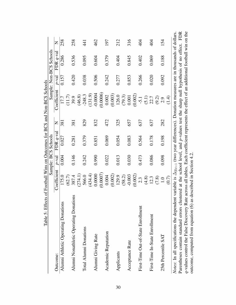
Table 5 reports propensity score results estimated separately for BCS and non-BCS

teams. In all regressions the dependent variable is specified in two-year differences (∆yit+1).

For most outcomes the estimated effect for BCS teams (the first column) is larger (or more

positive) than the estimated effect for non-BCS teams (the second column). However, for

in-state enrollment and SAT scores, there is a larger effect among non-BCS schools than

among BCS schools. Both these measures pertain to attracting students rather than satis-

fying alumni, and it is possible that winning seasons have a larger effect on visibility for

lower-profile non-BCS schools than for high-profile BCS schools.

16

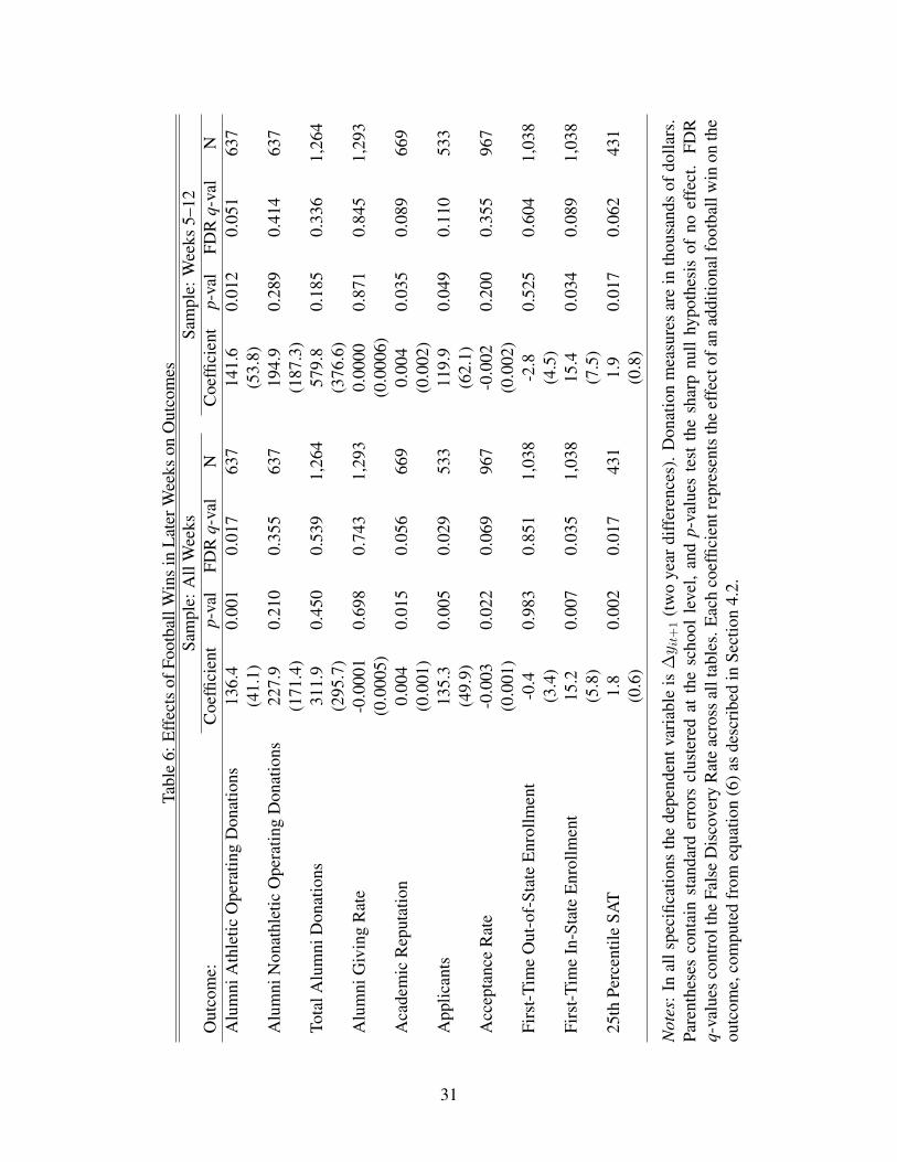
5.2 Effects Excluding Early Season Games

The propensity score design is particularly credible for games occurring later in the season.

At that point bookmakers have better knowledge of each team’s skill, and wins and losses

are closer to truly random after conditioning on bookmaker odds. As a robustness check

we estimate the results while excluding the first month of the season. The second set of

columns in Table 6 reports these results (the first set of columns reports the baseline results

from Table 4 for comparison).

In most cases the estimates change little when we exclude the first four games of the

season. Statistically significant effects remain for alumni athletic donations, academic rep-

utation, applicants, in-state enrollment, and SAT scores (the one exception is the acceptance

rate, which becomes statistically insignificant). Precision falls since there are now fewer

games used in the estimation sample, and many effects are only marginally significant af-

ter controlling FDR. Nevertheless, the similarity in the point estimates between the two

columns for outcomes that are statistically significant in the baseline results is reassuring.

5.3 Persistent Effects

The baseline results demonstrate that wins in year t affect outcomes in year t + 1. If wins

have persistent effects, then wins in year tmay also affect outcomes in year t+2 or beyond.

Let wit be wins in year t (i.e., wit =∑S

s=1wist). It is tempting to estimate the effect of wit

on yit+2 by simply replacing yit+1 with yit+2 in the “reduced form” equation, equation (5).

However, doing so overlooks the fact that winning in year t is correlated with winning in

year t+ 1, even after conditioning on the propensity score. This occurs for the same reason

that winning in week s is correlated with winning in week s+ 1 even after conditioning on

the propensity score – a win in week s can reveal that a team has more talent than expected.

Some of the estimated effect of winning in year t on yit+2 may thus result from increased

wins in year t+ 1.

We use the following procedure to estimate the effect of wit on yit+2 while holding

wit+1 constant. First, we replace yit+1 with yit+2 in equation (5) and estimate equation (6).

Denote this estimate as ψ̂; ψ̂ estimates the “reduced form” effect of wit on yit+2 without

17

controlling for changes in wit+1. Next, we estimate the relationship between wit and wit+1.

To do this we replace yit+1 with wit+1 in the “reduced form” equation (5) and estimate

equation (6). Denote this estimate as λ̂; λ̂ estimates the relationship between wit and wit+1

(after conditioning on the propensity score). Finally, we calculate θ̂ = ψ̂ − λ̂β̂, where β̂ is

the causal effect of wit on yit+1 (estimated in Section 5.1). In short, we adjust the reduced

form effect of wit on yit+2 to account for the fact that wit+1 is increasing in wit (i.e., λ̂) and

that wit+1 affects yit+2 (i.e., β̂).

The second set of columns in Table 7 reports estimates of θ̂, the effect of winning in

year t on outcomes in year t + 2. There is little evidence that winning has effects that

persist for two years. Most of the estimates are statistically insignificant and smaller than

comparable estimates from Table 4 (reproduced in the first set of columns). None are

statistically significant after controlling FDR. The effects of winning in year t appear to be

concentrated in the following year.

6 Conclusions

For FBS schools, winning football games increases alumni athletic donations, enhances a

school’s academic reputation, increases the number of applicants and in-state students, re-

duces acceptance rates, and raises average incoming SAT scores. The estimates imply that

large increases in team performance can have economically significant effects, particularly

in the area of athletic donations. Consider a school that improves its season wins by 5 games

(the approximate difference between a 25th percentile season and a 75th percentile season).

Changes of this magnitude occur approximately 8% of the time over a one-year period and

13% of the time over a two-year period. This school may expect alumni athletic donations

to increase by $682,000 (28%), applications to increase by 677 (5%), the acceptance rate

to drop by 1.5 percentage points (2%), in-state enrollment to increase by 76 students (3%),

and incoming 25th percentile SAT scores to increase by 9 points (1%). These estimates

are equal to or larger than comparable estimates from the existing literature. For example,

among studies that found significant effects, a 5-win increase in team performance was

associated with a 2.1% to 2.5% increase in applications (Murphy and Trandel 1994; Pope

18

and Pope 2009) and a $687,000 increase in restricted donations (Humphreys and Mondello

2007).

Do these effects imply that investing in team quality generates positive net benefits for

an FBS school? Answering this question is difficult because we do not know the causal

relationship between team investments and team wins. Nevertheless, we consider a simple

back-of-the-envelope calculation to establish the potential return on team investments.

Orszag and Israel (2009) report that a $1 million increase in “football team expendi-

tures” is associated with a 6.7 percentage point increase in football winning percentage

(0.8 games). If we interpret this relationship as causal, it implies that a $1 million in-

vestment in football team expenditures increases alumni athletic donations by $109,000,

increases annual applications by 108, and increases the average incoming SAT score by 1.4

points. These effects seem too modest by themselves to offset the additional expenditures.

However, if increases in team expenditures generate commensurate increases in athletic

revenue (another finding in Orszag and Israel (2009), though a portion of this relationship

is presumably due to reverse causality), then the effects estimated here represent a “bonus”

that the school gets on top of the increased athletic revenue.

Two additional caveats apply when interpreting our results. First, we estimate the ef-

fects of unexpected wins. If a school invests in its football program and improves its record,

alumni and applicant expectations will eventually change. The effects of a persistent in-

crease in season wins may therefore differ from the effects we estimate here.

Second, the effects we observe likely operate through two channels. One channel is

team quality – a team that plays well is more enjoyable to watch than a team that plays

poorly, even holding constant the game’s outcome. This is in part why the NFL can charge

much higher ticket prices than competing leagues that employ less skilled players (e.g.,

the Arena Football League). The second channel is winning itself – fans and alumni enjoy

winning games regardless of how well the team plays. Team records, however, are by def-

inition a zero-sum game; one team’s win is another team’s loss. The effects demonstrated

here thus do not change the “arms race” nature of team investment, as each team purchases

its wins at the cost of other teams. While improving the overall level of play in the NCAA

may attract more fans and alumni support through the first channel, it cannot have any ef-

19

fect on the second channel. A simultaneous investment of $1 million in each BCS football

team will likely generate smaller effects on donations and applications than the estimates

presented in this paper.

These caveats notwithstanding, we demonstrate that big-time athletic success can at-

tract donations and students. We do so by extending the propensity score design to a dy-

namic setting in which multiple treatments occur at different points in time. In this setting

the propensity score for any given treatment depends on the realized values of previous

treatments. We apply this framework in a context in which the ignorability assumption

is likely to hold and in which previous research has generated inconsistent conclusions.

While the ignorability assumption does not apply in many circumstances, in those that it

does these tools may facilitate estimation of causal effects.

20

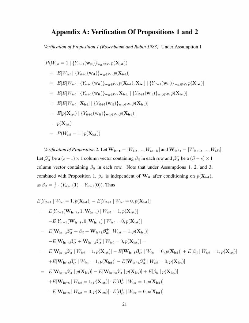
Appendix A: Verification Of Propositions 1 and 2

Verification of Proposition 1 (Rosenbaum and Rubin 1983). Under Assumption 1

P (Wist = 1 | {Yit+1(wit)}wit∈W , p(Xist))

= E[Wist | {Yit+1(wit)}wit∈W , p(Xist)]

= E[E[Wist | {Yit+1(wit)}wit∈W , p(Xist),Xist] | {Yit+1(wit)}wit∈W , p(Xist)]

= E[E[Wist | {Yit+1(wit)}wit∈W ,Xist] | {Yit+1(wit)}wit∈W , p(Xist)]

= E[E[Wist |Xist] | {Yit+1(wit)}wit∈W , p(Xist)]

= E[p(Xist) | {Yit+1(wit)}wit∈W , p(Xist)]

= p(Xist)

= P (Wist = 1 | p(Xist))

Verification of Proposition 2. Let Wis−t = [Wi1t, ...,Wis−1t] and Wis+t = [Wis+1t, ...,WiSt].

Let β−it be a (s− 1)× 1 column vector containing βit in each row and β+

it be a (S − s)× 1

column vector containing βit in each row. Note that under Assumptions 1, 2, and 3,

combined with Proposition 1, βit is independent of Wit after conditioning on p(Xist),

as βit = 1S· (Yit+1(1)− Yit+1(0)). Thus

E[Yit+1 |Wist = 1, p(Xist)]− E[Yit+1 |Wist = 0, p(Xist)]

= E[Yit+1(Wis−t, 1,Wis+t) |Wist = 1, p(Xist)]

−E[Yit+1(Wis−t, 0,Wis+t) |Wist = 0, p(Xist)]

= E[Wis−tβ−it + βit + Wis+tβ

+it |Wist = 1, p(Xist)]

−E[Wis−tβ−it + Wis+tβ

+it |Wist = 0, p(Xist)] =

= E[Wis−tβ−it |Wist = 1, p(Xist)]− E[Wis−tβ

−it |Wist = 0, p(Xist)] + E[βit |Wist = 1, p(Xist)]

+E[Wis+tβ+it |Wist = 1, p(Xist)]− E[Wis+tβ

+it |Wist = 0, p(Xist)]

= E[Wis−tβ−it | p(Xist)]− E[Wis−tβ

−it | p(Xist)] + E[βit | p(Xist)]

+E[Wis+t |Wist = 1, p(Xist)] · E[β+it |Wist = 1, p(Xist)]

−E[Wis+t |Wist = 0, p(Xist)] · E[β+it |Wist = 0, p(Xist)]

21

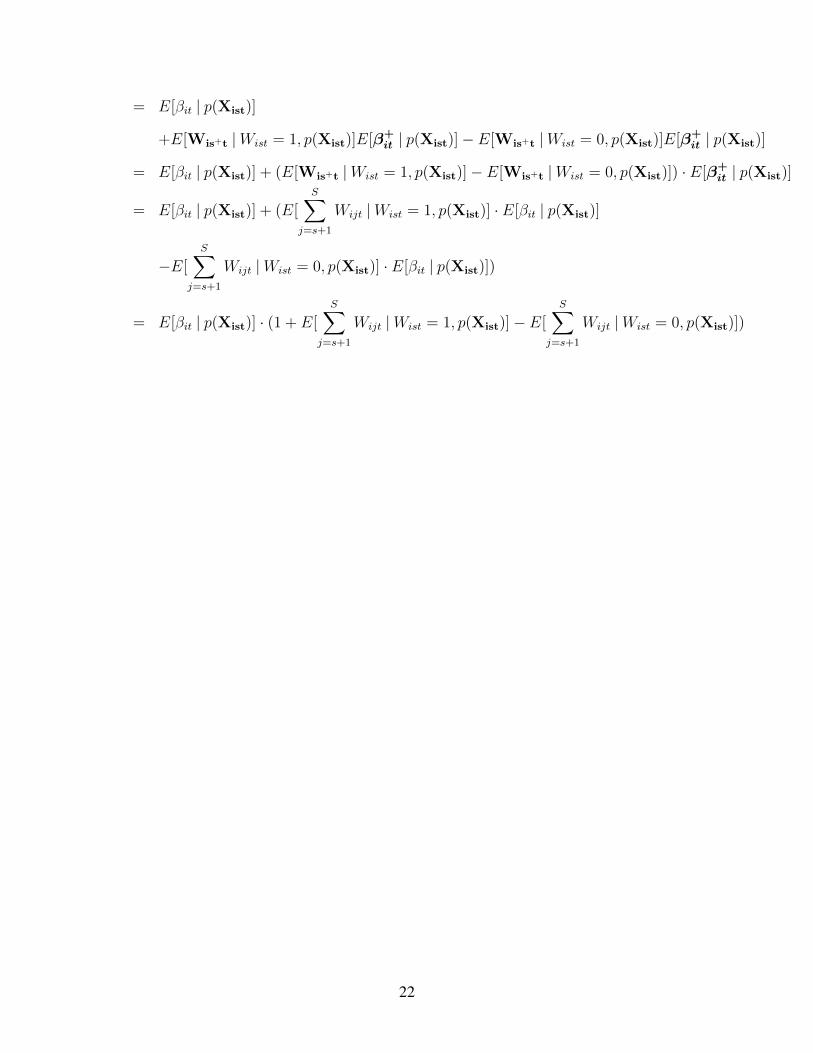
= E[βit | p(Xist)]

+E[Wis+t |Wist = 1, p(Xist)]E[β+it | p(Xist)]− E[Wis+t |Wist = 0, p(Xist)]E[β+

it | p(Xist)]

= E[βit | p(Xist)] + (E[Wis+t |Wist = 1, p(Xist)]− E[Wis+t |Wist = 0, p(Xist)]) · E[β+it | p(Xist)]

= E[βit | p(Xist)] + (E[S∑

j=s+1

Wijt |Wist = 1, p(Xist)] · E[βit | p(Xist)]

−E[S∑

j=s+1

Wijt |Wist = 0, p(Xist)] · E[βit | p(Xist)])

= E[βit | p(Xist)] · (1 + E[S∑

j=s+1

Wijt |Wist = 1, p(Xist)]− E[S∑

j=s+1

Wijt |Wist = 0, p(Xist)])

22

References

M. L. Anderson. Multiple inference and gender differences in the effects of early inter-

vention: A reevaluation of the abecedarian, perry preschool, and early training projects.

Journal of the American Statistical Association, 103(484):1481–1495, Dec. 2008.

J. D. Angrist and G. W. Imbens. Two-Stage least squares estimation of average causal

effects in models with variable treatment intensity. Journal of the American Statistical

Association, 90(430):431–442, 1995.

J. D. Angrist and G. M. Kuersteiner. Causal effects of monetary shocks: Semiparametric

conditional independence tests with a multinomial propensity score. Review of Eco-

nomics and Statistics, 93(3):725–747, 2011.

R. A. Baade and J. O. Sundberg. Fourth down and gold to go? Assessing the link between

athletics and alumni giving. Social Science Quarterly, 77(4):789–803, 1996.

Y. Benjamini, A. M. Krieger, and D. Yekutieli. Adaptive linear step-up procedures that

control the false discovery rate. Biometrika, 93(3):491–507, Sept. 2006.

J. Bound, D. Jaeger, and R. Baker. Problems with instrumental variables estimation when

the correlation between the instruments and the endogeneous explanatory variable is

weak. Journal of the American Statistical Association, 90(430):443–450, 1995.

G. W. Brooker and T. D. Klastorin. To the victors belong the spoils? College athletics and

alumni giving. Social Science Quarterly, 62(4):744–50, Dec. 1981.

D. Card and G. B. Dahl. Family violence and football: The effect of unexpected emotional

cues on violent behavior. The Quarterly Journal of Economics, 126(1):103–143, Feb.

2011.

R. H. Dehejia and S. Wahba. Causal effects in nonexperimental studies: Reevaluating the

evaluation of training programs. Journal of the American Statistical Association, 94

(448):1053–1062, 1999.

23

D. L. Fulks. Revenues and expenses 2004–2010: NCAA Division I intercollegiate athletics

programs report. Technical report, National Collegiate Athletic Association, Indianapo-

lis, IN, 2011.

M. E. Glickman and H. S. Stern. A State-Space model for national football league scores.

Journal of the American Statistical Association, 93(441):25–35, 1998.

P. W. Grimes and G. A. Chressanthis. Alumni contributions to academics. American

Journal of Economics and Sociology, 53(1):27–40, 1994.

K. Hirano and G. Imbens. The propensity score with continuous treatments. In A. Gel-

man and X.-L. Meng, editors, Applied Bayesian Modeling and Causal Inference from

Incomplete-Data Perspectives: An Essential Journey with Donald Rubin’s Statistical

Family, chapter 7, pages 73–84. John Wiley and Sons, Ltd, 2004.

K. Hirano, G. Imbens, and G. Ridder. Efficient estimation of average treatment effects

using the estimated propensity score. Econometrica, 71(4):1161–1189, 2003.

B. R. Humphreys and M. Mondello. Intercollegiate athletic success and donations at NCAA

division i institutions. Journal of Sport Management, 21(2):265–280, 2007.

K. Imai and D. A. van Dyk. Causal inference with general treatment regimes. Journal of

the American Statistical Association, 99(467):854–866, Sept. 2004.

R. J. LaLonde. Evaluating the econometric evaluations of training programs with experi-

mental data. American Economic Review, 76(4):604–20, 1986.

S. Levitt. Why are gambling markets organised so differently from financial markets?

Economic Jounal, 114(495):223–246, April 2004.

J. Meer and H. S. Rosen. The impact of athletic performance on alumni giving: An analysis

of microdata. Economics of Education Review, 28(3):287–294, June 2009.

R. G. Murphy and G. A. Trandel. The relation between a university’s football record and

the size of its applicant pool. Economics of Education Review, 13(3):265–270, Sept.

1994.

24

J. Orszag and M. Israel. The empirical effects of collegiate athletics: An update based on

2004-2007 data. Technical report, Compass Lexecon, 2009.

D. G. Pope and J. C. Pope. The impact of college sports success on the quantity and quality

of student applications. Southern Economic Journal, 75(3), 2009.

P. R. Rosenbaum and D. B. Rubin. The central role of the propensity score in observational

studies for causal effects. Biometrika, 70(1):41 –55, Apr. 1983.

D. Rubin. Randomization analysis of experimental data: The fisher randomization test

comment. Journal of the American Statistical Association, 75(371):591–593, 1980.

L. Sigelman and S. Bookheimer. Is it whether you win or lose? Monetary contributions

to Big-Time college athletic programs. Social Science Quarterly, 64(2):347–59, June

1983.

L. Sigelman and R. Carter. Win one for the giver? Alumni giving and Big-Time college

sports. Social Science Quarterly, 60(2):284–94, 1979.

J. Smith and P. Todd. Does matching overcome lalonde’s critique of nonexperimental

estimators? Journal of Econometrics, 125(1-2):305–353, 2005.

H. Stern. On the probability of winning a football game. The American Statistician, 45(3):

179–183, 1991.

H. S. Stern. Point spread and odds betting: Baseball, basketball, and american football.

In D. B. Hausch and W. T. Ziemba, editors, Handbook of Sports and Lottery Markets,

pages 223–237. Elsevier, Oxford, UK, 2008.

I. B. Tucker. A reexamination of the effect of big-time football and basketball success

on graduation rates and alumni giving rates. Economics of Education Review, 23(6):

655–661, Dec. 2004.

S. E. Turner, L. A. Meserve, and W. G. Bowen. Winning and giving: Football results and

alumni giving at selective private colleges and universities. Social Science Quarterly, 82

(4):812–826, 2001.

25

T abl

e1:

Sum

mar

ySt

atis

tics

All

Team

sB

CS

Non

-BC

SD

ates

Var

iabl

e:M

ean

NM

ean

NM

ean

NA

vaila

ble

Sour

ceSe

ason

Win

s5.

42,

360

5.9

1,47

74.

588

319

87–2

009

Cov

ers.

com

(2.7

)(2

.6)

(2.5

)Se

ason

Gam

es10

.72,

360

10.7

1,47

710

.588

319

87–2

009

Cov

ers.

com

(0.9

)(0

.8)

(1.0

)E

xpec

ted

Win

s5.

42,

360

5.9

1,47

74.

588

319

87–2

009

Cov

ers.

com

(2.1

)(2

.1)

(1.8

)A

lum

niA

thle

ticO

pera

ting

Don

atio

ns$2

,439

925

$3,8

2953

4$5

4039

119

99–2

009

VSE

(3,2

72)

(3,7

05)

(0,5

93)

Alu

mni

Non

athl

etic

Ope

ratin

gD

onat

ions

$7,1

3692

5$1

1,00

053

4$1

,912

391

1999

–200

9V

SE(1

2,10

0)(1

4,50

0)(3

,684

)To

talA

lum

niD

onat

ions

$18,

800

1,79

3$2

7,00

01,

129

$4,9

0866

419

90–2

009

VSE

(26,

700)

(30,

400)

(6,5

20)

Alu

mni

Giv

ing

Rat

e0.

141

1,83

70.

165

1,14

10.

102

696

1990

–200

9V

SE(0

.078

)(0

.077

)(0

.061

)A

cade

mic

Rep

utat

ion

3.22

1,04

43.

4770

12.

7134

319

97–2

008

US

New

s(0

.63)

(0.5

5)(0

.44)

App

lican

ts13

,748

840

16,6

2350

29,

479

338

1999

–200

7IP

ED

S(8

,187

)(8

,058

)(6

,305

)A

ccep

tanc

eR

ate

0.69

81,

591

0.66

91,

064

0.75

652

719

88–2

008

US

New

s(0

.181

)(0

.184

)(0

.159

)Fi

rst-

Tim

eO

ut-o

f-St

ate

Enr

ollm

ent

802

1,49

81,

015

913

469

585

1986

–200

8IP

ED

S(6

32)

(596

)(5

36)

Firs

t-Ti

me

In-S

tate

Enr

ollm

ent

2,54

11,

498

2,81

491

32,

115

585

1986

–200

8IP

ED

S(1

,404

)(1

,522

)(1

,067

)25

thPe

rcen

tile

SAT

1,05

471

81,

097

451

981

267

1999

–200

8IP

ED

S(1

19)

(103

)(1

08)

Not

es:

Don

atio

nm

easu

res

are

inth

ousa

nds

ofdo

llars

.Pa

rent

hese

sco

ntai

nst

anda

rdde

viat

ions

.O

neob

serv

atio

nis

asi

ngle

scho

olfo

rasi

ngle

year

.

26

T abl

e2:

OL

San

dL

ongi

tudi

nalR

elat

ions

hips

Bet

wee

nFo

otba

llW

ins

and

Out

com

esO

LS

Rel

atio

nshi

psL

ongi

tudi

nalR

elat

ions

hips

Out

com

e:C

oeffi

cien

tp-

val

FDR

q-va

lN

Coe

ffici

ent

p-va

lFD

Rq-

val

NA

lum

niA

thle

ticO

pera

ting

Don

atio

ns34

0.4

0.00

10.

017

914

74.0

0.00

20.

017

698

(99.

8)(2

3.2)

Alu

mni

Non

athl

etic

Ope

ratin

gD

onat

ions

161.

60.

527

0.60

491

411

7.2

0.24

60.

381

698

(254

.7)

(100

.3)

Tota

lAlu

mni

Don

atio

ns96

0.1

0.03

90.

095

1,77

120

7.7

0.15

00.

281

1,40

3(4

60.6

)(1

43.2

)A

lum

niG

ivin

gR

ate

0.00

250.

150

0.28

11,

814

0.00

030.

358

0.49

71,

437

(0.0

017)

(0.0

003)

Aca

dem

icR

eput

atio

n0.

015

0.36

30.

497

1,03

10.

002

0.02

90.

082

727

(0.0

16)

(0.0

01)

App

lican

ts31

4.8

0.10

40.

204

826

103.

60.

000

0.00

158

5(1

92.0

)(2

6.8)

Acc

epta

nce

Rat

e-0

.001

0.84

10.

845

1,56

2-0

.002

0.00

90.

041

1,08

4(0

.004

)(0

.001

)Fi

rst-

Tim

eO

ut-o

f-St

ate

Enr

ollm

ent

34.4

0.00

20.

017

1,39

72.

90.

262

0.40

11,

076

(11.

0)(2

.6)

Firs

t-Ti

me

In-S

tate

Enr

ollm

ent

91.3

0.00

40.

027

1,39

716

.60.

001

0.01

71,

076

(31.

3)(4

.9)

25th

Perc

entil

eSA

T3.

10.

355

0.49

770

70.

60.

079

0.16

547

4(3

.3)

(0.3

)

Not

es:

Don

atio

nm

easu

res

are

inth

ousa

nds

ofdo

llars

.Pa

rent

hese

sco

ntai

nst

anda

rder

rors

clus

tere

dat

the

scho

olle

vel.

FDR

q-va

lues

cont

rol

the

Fals

eD

isco

very

Rat

eac

ross

all

tabl

es.

Eac

hco

effic

ient

isfr

oma

sepa

rate

regr

essi

onin

whi

chth

eou

tcom

eis

regr

esse

don

seas

onw

ins.

All

regr

essi

ons

incl

ude

seas

onga

mes

and

year

fixed

effe

cts

asco

ntro

ls,a

ndal

lvar

iabl

esin

long

itudi

nal

regr

essi

ons

are

diff

eren

ced

over

two

year

s(s

eeSe

ctio

n3.

2).

27

T abl

e3:

OL

San

dL

ongi

tudi

nalR

elat

ions

hips

Bet

wee

nFo

otba

llW

ins

and

Out

com

esfo

rBC

SSc

hool

sO

LS

Rel

atio

nshi

psL

ongi

tudi

nalR

elat

ions

hips

Out

com

e:C

oeffi

cien

tp-

val

FDR

q-va

lN

Coe

ffici

ent

p-va

lFD

Rq-

val

NA

lum

niA

thle

ticO

pera

ting

Don

atio

ns35

5.6

0.00

80.

038

532

121.

90.

002

0.01

741

7(1

29.5

)(3

7.3)

Alu

mni

Non

athl

etic

Ope

ratin

gD

onat

ions

-427

.40.

349

0.49

753

219

1.5

0.28

10.

405

417

(452

.6)

(175

.7)

Tota

lAlu

mni

Don

atio

ns37

.10.

955

0.85

01,

126

328.

20.

131

0.25

692

0(6

59.1

)(2

14.7

)A

lum

niG

ivin

gR

ate

-0.0

010

0.68

60.

743

1,13

80.

0004

0.41

00.

526

926

(0.0

024)

(0.0

004)

Aca

dem

icR

eput

atio

n-0

.016

0.37

80.

517

699

0.00

20.

028

0.08

251

9(0

.018

)(0

.001

)A

pplic

ants

108.

00.

633

0.72

050

012

1.3

0.00

20.

017

360

(225

.2)

(37.

4)A

ccep

tanc

eR

ate

0.00

00.

940

0.85

01,

061

-0.0

030.

001

0.01

774

2(0

.005

)(0

.001

)Fi

rst-

Tim

eO

ut-o

f-St

ate

Enr

ollm

ent

3.0

0.82

40.

845

851

7.2

0.00

20.

017

654

(13.

3)(2

.2)

Firs

t-Ti

me

In-S

tate

Enr

ollm

ent

88.4

0.06

00.

131

851

21.4

0.00

20.

017

654

(46.

2)(6

.6)

25th

Perc

entil

eSA

T-2

.00.

623

0.71

144

90.

30.

458

0.54

531

1(4

.0)

(0.4

)N

otes

:D

onat

ion

mea

sure

sar

ein

thou

sand

sof

dolla

rs.

Pare

nthe

ses

cont

ain

stan

dard

erro

rscl

uste

red

atth

esc

hool

leve

l.FD

Rq-

valu

esco

ntro

lth

eFa

lse

Dis

cove

ryR

ate

acro

ssal

lta

bles

.E

ach

coef

ficie

ntis

from

ase

para

tere

gres

sion

inw

hich

the

depe

nden

tva

riab

leis

regr

esse

don

seas

onw

ins.

All

regr

essi

ons

incl

ude

seas

onga

mes

and

year

fixed

effe

cts

asco

ntro

ls,a

ndal

lvar

iabl

esin

long

itudi

nalr

egre

ssio

nsar

edi

ffer

ence

dov

ertw

oye

ars

(see

Sect

ion

3.2)

.The

sam

ple

isre

stri

cted

toB

CS

scho

ols.

28

Tabl

e4:

Eff

ects

ofFo

otba

llW

ins

onO

utco

mes

Dep

ende

ntV

aria

ble:y i

t+1

Dep

ende

ntV

aria

ble:

∆y i

t+1

Out

com

e:C

oeffi

cien

tp-

val

FDR

q-va

lN

Coe

ffici

ent

p-va

lFD

Rq-

val

NA

lum

niA

thle

ticO

pera

ting

Don

atio

ns17

5.1

0.02

90.

082

818

136.

40.

001

0.01

763

7(6

7.6)

(41.

1)A

lum

niN

onat

hlet

icO

pera

ting

Don

atio

ns64

.30.

894

0.84

581

822

7.9

0.21

00.

355

637

(283

.6)

(171

.4)

Tota

lAlu

mni

Don

atio

ns52

7.1

0.22

80.

377

1,56

531

1.9

0.45

00.

539

1,26

4(4

29.4

)(2

95.7

)A

lum

niG

ivin

gR

ate

0.00

170.

155

0.28

61,

605

-0.0

001

0.69

80.

743

1,29

3(0

.001

2)(0

.000

5)A

cade

mic

Rep

utat

ion

-0.0

030.

717

0.74

391

90.

004

0.01

50.

056

669

(0.0

13)

(0.0

02)

App

lican

ts4.

90.

942

0.85

074

013

5.3

0.00

50.

029

533

(184

.3)

(49.

9)A

ccep

tanc

eR

ate

0.00

00.

955

0.85

01,

379

-0.0

030.

022

0.06

996

7(0

.003

)(0

.001

)Fi

rst-

Tim

eO

ut-o

f-St

ate

Enr

ollm

ent

11.9

0.23

60.

379

1,23

7-0

.40.

983

0.85

11,

038

(11.

1)(3

.4)

Firs

t-Ti

me

In-S

tate

Enr

ollm

ent

10.5

0.78

30.

838

1,23

715

.20.

007

0.03

51,

038

(25.

0)(5

.8)

25th

Perc

entil

eSA

T2.

60.

387

0.52

564

01.

80.

002

0.01

743

1(2

.9)

(0.6

)

Not

es:

Don

atio

nm

easu

res

are

inth

ousa

nds

ofdo

llars

.Pa

rent

hese

sco

ntai

nst

anda

rder

rors

clus

tere

dat

the

scho

olle

vel,

and

p-va

lues

test

the

shar

pnu

llhy

poth

esis

ofno

effe

ct.

FDR

q-va

lues

cont

rolt

heFa

lse

Dis

cove

ryR

ate

acro

ssal

ltab

les.

Eac

hco

effic

ient

repr

esen

tsth

eef

fect

ofan

addi

tiona

lfoo

tbal

lwin

onth

eou

tcom

e,co

mpu

ted

from

equa

tion

(6)a

sde

scri

bed

inSe

ctio

n4.

2.

29

T abl

e5:

Eff

ects

ofFo

otba

llW

ins

onO

utco

mes

forB

CS

and

Non

-BC

SSc

hool

sSa

mpl

e:B

CS

Scho

ols

Sam

ple:

Non

-BC

SSc

hool

sO

utco

me:

Coe

ffici

ent

p-va

lFD

Rq-

val

NC

oeffi

cien

tp-

val

FDR

q-va

lN

Alu

mni

Ath

letic

Ope

ratin

gD

onat

ions

175.

00.

004

0.02

738

117

.70.

157

0.28

625

8(6

2.7)

(11.

7)A

lum

niN

onat

hlet

icO

pera

ting

Don

atio

ns38

7.4

0.14

60.

281

381

39.9

0.42

00.

536

258

(274

.1)

(46.

8)To

talA

lum

niD

onat

ions

566.

00.

242

0.37

982

9-2

48.3

0.03

80.

095

441

(434

.4)

(131

.9)

Alu

mni

Giv

ing

Rat

e0.

0000

0.99

00.

851

832

-0.0

004

0.50

60.

604

462

(0.0

007)

(0.0

006)

Aca

dem

icR

eput

atio

n0.

004

0.02

20.

069

472

0.00

20.

242

0.37

919

7(0

.002

)(0

.003

)A

pplic

ants

129.

90.

013

0.05

432

512

6.0

0.27

70.

404

212

(58.

2)(7

9.3)

Acc

epta

nce

Rat

e-0

.003

0.03

00.

083

657

0.00

10.

853

0.84

531

6(0

.002

)(0

.002

)Fi

rst-

Tim

eO

ut-o

f-St

ate

Enr

ollm

ent

2.3

0.47

30.

564

637

-5.1

0.26

60.

402

404

(4.8

)(5

.1)

Firs

t-Ti

me

In-S

tate

Enr

ollm

ent

12.3

0.08

60.

178

637

22.7

0.02

00.

069

404

(7.8

)(9

.2)

25th

Perc

entil

eSA

T1.

00.

098

0.19

828

22.

90.

092

0.18

815

4(0

.7)

(1.4

)N

otes

:In

alls

peci

ficat

ions

the

depe

nden

tvar

iabl

eis

∆y i

t+1

(tw

oye

ardi

ffer

ence

s).

Don

atio

nm

easu

res

are

inth

ousa

nds

ofdo

llars

.Pa

rent

hese

sco

ntai

nst

anda

rder

rors

clus

tere

dat

the

scho

olle

vel,

and

p-va

lues

test

the

shar

pnu

llhy

poth

esis

ofno

effe

ct.

FDR

q-va

lues

cont

rolt

heFa

lse

Dis

cove

ryR

ate

acro

ssal

ltab

les.

Eac

hco

effic

ient

repr

esen

tsth

eef

fect

ofan

addi

tiona

lfoo

tbal

lwin

onth

eou

tcom

e,co

mpu

ted

from

equa

tion

(6)a

sde

scri

bed

inSe

ctio

n4.

2.

30

T abl

e6:

Eff

ects

ofFo

otba

llW

ins

inL

ater

Wee

kson

Out

com

esSa

mpl

e:A

llW

eeks

Sam

ple:

Wee

ks5–

12O

utco

me:

Coe

ffici

ent

p-va

lFD

Rq-

val

NC

oeffi

cien

tp-

val

FDR

q-va

lN

Alu

mni

Ath

letic

Ope

ratin

gD

onat

ions

136.

40.

001

0.01

763

714

1.6

0.01

20.

051

637

(41.

1)(5

3.8)

Alu

mni

Non

athl

etic

Ope

ratin

gD

onat

ions

227.

90.

210

0.35

563

719

4.9

0.28

90.

414

637

(171

.4)

(187

.3)

Tota

lAlu

mni

Don

atio

ns31

1.9

0.45

00.

539

1,26

457

9.8

0.18

50.

336

1,26

4(2

95.7

)(3

76.6

)A

lum

niG

ivin

gR

ate

-0.0

001

0.69

80.

743

1,29

30.

0000

0.87

10.

845

1,29

3(0

.000

5)(0

.000

6)A

cade

mic

Rep

utat

ion

0.00

40.

015

0.05

666

90.

004

0.03

50.

089

669

(0.0

01)

(0.0

02)

App

lican

ts13

5.3

0.00

50.

029

533

119.

90.

049

0.11

053

3(4

9.9)

(62.

1)A

ccep

tanc

eR

ate

-0.0

030.

022

0.06

996

7-0

.002

0.20

00.

355

967

(0.0

01)

(0.0

02)

Firs

t-Ti

me

Out

-of-

Stat

eE

nrol

lmen

t-0

.40.

983

0.85

11,

038

-2.8

0.52

50.

604

1,03

8(3

.4)

(4.5

)Fi

rst-

Tim

eIn

-Sta

teE

nrol

lmen

t15

.20.

007

0.03

51,

038

15.4

0.03

40.

089

1,03

8(5

.8)

(7.5

)25

thPe

rcen

tile

SAT

1.8

0.00

20.

017

431

1.9

0.01

70.

062

431

(0.6

)(0

.8)

Not

es:

Inal

lspe

cific

atio

nsth

ede

pend

entv

aria

ble

is∆y i

t+1

(tw

oye

ardi

ffer

ence

s).

Don

atio

nm

easu

res

are

inth

ousa

nds

ofdo

llars

.Pa

rent

hese

sco

ntai

nst

anda

rder

rors

clus

tere

dat

the

scho

olle

vel,

and

p-va

lues

test

the

shar

pnu

llhy

poth

esis

ofno

effe

ct.

FDR

q-va

lues

cont

rolt

heFa

lse

Dis

cove

ryR

ate

acro

ssal

ltab

les.

Eac

hco

effic

ient

repr

esen

tsth

eef

fect

ofan

addi

tiona

lfoo

tbal

lwin

onth

eou

tcom

e,co

mpu

ted

from

equa

tion

(6)a

sde

scri

bed

inSe

ctio

n4.

2.

31

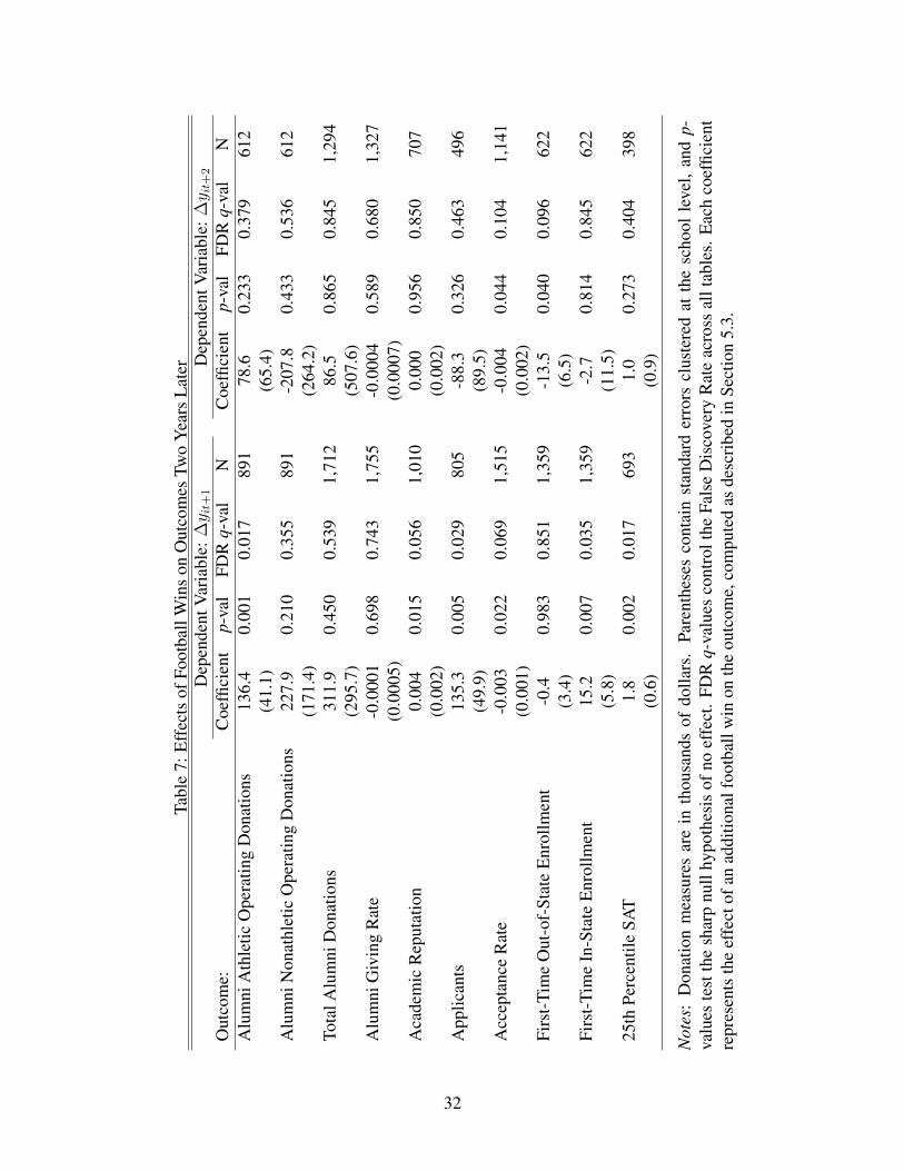
Tabl

e7:

Eff

ects

ofFo

otba

llW

ins

onO

utco

mes

Two

Yea

rsL

ater

Dep

ende

ntV

aria

ble:

∆y i

t+1

Dep

ende

ntV

aria

ble:

∆y i

t+2

Out

com

e:C

oeffi

cien

tp-

val

FDR

q-va

lN

Coe

ffici

ent

p-va

lFD

Rq-

val

NA

lum

niA

thle

ticO

pera

ting

Don

atio

ns13

6.4

0.00

10.

017

891

78.6

0.23

30.

379

612

(41.

1)(6

5.4)

Alu

mni

Non

athl

etic

Ope

ratin

gD

onat

ions

227.

90.

210

0.35

589

1-2

07.8

0.43

30.

536

612

(171

.4)

(264

.2)

Tota

lAlu

mni

Don

atio

ns31

1.9

0.45

00.

539

1,71

286

.50.

865

0.84

51,

294

(295

.7)

(507

.6)

Alu

mni

Giv

ing

Rat

e-0

.000

10.

698

0.74

31,

755

-0.0

004

0.58

90.

680

1,32

7(0

.000

5)(0

.000

7)A

cade

mic

Rep

utat

ion

0.00

40.

015

0.05

61,

010

0.00

00.

956

0.85

070

7(0

.002

)(0

.002

)A

pplic

ants

135.

30.

005

0.02

980

5-8

8.3

0.32

60.

463

496

(49.

9)(8

9.5)

Acc

epta

nce

Rat

e-0

.003

0.02

20.

069

1,51

5-0

.004

0.04

40.

104

1,14

1(0

.001

)(0

.002

)Fi

rst-

Tim

eO

ut-o

f-St

ate

Enr

ollm

ent

-0.4

0.98

30.

851

1,35

9-1

3.5

0.04

00.

096

622

(3.4

)(6

.5)

Firs

t-Ti

me

In-S

tate

Enr

ollm

ent

15.2

0.00

70.

035

1,35

9-2

.70.

814

0.84

562

2(5

.8)

(11.

5)25

thPe

rcen

tile

SAT

1.8

0.00

20.

017

693

1.0

0.27

30.

404

398

(0.6

)(0

.9)

Not

es:

Don

atio

nm

easu

res

are

inth

ousa

nds

ofdo

llars

.Pa

rent

hese

sco

ntai

nst

anda

rder

rors

clus

tere

dat

the

scho

olle

vel,

and

p-va

lues

test

the

shar

pnu

llhy

poth

esis

ofno

effe

ct.

FDR

q-va

lues

cont

rolt

heFa

lse

Dis

cove

ryR

ate

acro

ssal

ltab

les.

Eac

hco

effic

ient

repr

esen

tsth

eef

fect

ofan

addi

tiona

lfoo

tbal

lwin

onth

eou

tcom

e,co

mpu

ted

asde

scri

bed

inSe

ctio

n5.

3.

32

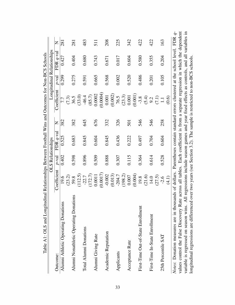
T abl

eA

1:O

LS

and

Lon

gitu

dina

lRel

atio

nshi

psB

etw

een

Foot

ball

Win

san

dO

utco

mes

forN

on-B

CS

Scho

ols

OL

SR

elat

ions

hips

Lon

gitu

dina

lRel

atio

nshi

psO

utco

me:

Coe

ffici

ent

p-va

lFD

Rq-

val

NC

oeffi

cien

tp-

val

FDR

q-va

lN

Alu

mni

Ath

letic

Ope

ratin

gD

onat

ions

19.6

0.40

20.

525

382

7.7

0.29

90.

427

281

(23.

2)(7

.3)

Alu

mni

Non

athl

etic

Ope

ratin

gD

onat

ions

59.8

0.59

80.

683

382

36.5

0.27

50.

404

281

(112

.5)

(33.

0)To

talA

lum

niD

onat

ions

-22.

70.

896

0.84

564

5-4

6.4

0.59

10.

680

483

(172

.7)

(85.

7)A

lum

niG

ivin

gR

ate

0.00

110.

509

0.60

467

60.

0002

0.66

50.

743

511

(0.0

017)

(0.0

004)

Aca

dem

icR

eput

atio

n-0

.002

0.88

80.

845

332

0.00

10.

568

0.67

120

8(0

.013

)(0

.002

)A

pplic

ants

-204

.70.

307

0.43

632

676

.50.

002

0.01

722

5(1

98.2

)(2

3.3)

Acc

epta

nce

Rat

e0.

007

0.11

50.

222

501

0.00

10.

520

0.60

434

2(0

.004

)(0

.001

)Fi

rst-

Tim

eO

ut-o

f-St

ate

Enr

ollm

ent

19.8

0.36

40.

497

546

-3.8

0.48

60.

580

422

(21.

6)(5

.4)

Firs

t-Ti

me

In-S

tate

Enr

ollm

ent

14.0

0.61

40.

704

546

9.2

0.20

10.

355

422

(27.

5)(7

.1)

25th

Perc

entil

eSA

T-2

.60.

528

0.60

425

81.

10.

105

0.20

416

3(4

.1)

(0.6

)N

otes

:D

onat

ion

mea

sure

sar

ein

thou

sand

sof

dolla

rs.

Pare

nthe

ses

cont

ain

stan

dard

erro

rscl

uste

red

atth

esc

hool

leve

l.FD

Rq-

valu

esco

ntro

lth

eFa

lse

Dis

cove

ryR

ate

acro

ssal

lta

bles

.E

ach

coef

ficie

ntis

from

ase

para

tere

gres

sion

inw

hich

the

depe

nden

tva

riab

leis

regr

esse

don

seas

onw

ins.

All

regr

essi

ons

incl

ude

seas

onga

mes

and

year

fixed

effe

cts

asco

ntro

ls,a

ndal

lvar

iabl

esin

long

itudi

nalr

egre

ssio

nsar

edi

ffer

ence

dov

ertw

oye

ars

(see

Sect

ion

3.2)

.The

sam

ple

isre

stri

cted

tono

n-B

CS

scho

ols.

33