The Big Match in Small Space

Kristoffer Arnsfelt Hansen∗1, Rasmus Ibsen-Jensen2, and Michal Koucky†3

1Aarhus University2IST Austria

3Charles University, Prague

April 26, 2016

Abstract

In this paper we study how to play (stochastic) games optimally using little space. We focuson repeated games with absorbing states, a type of two-player, zero-sum concurrent mean-payoffgames. The prototypical example of these games is the well known Big Match of Gillete (1957).These games may not allow optimal strategies but they always have ε-optimal strategies. Inthis paper we design ε-optimal strategies for Player 1 in these games that use only O(log log T )space. Furthermore, we construct strategies for Player 1 that use space s(T ), for an arbitrarysmall unbounded non-decreasing function s, and which guarantee an ε-optimal value for Player1 in the limit superior sense. The previously known strategies use space Ω(log T ) and it wasknown that no strategy can use constant space if it is ε-optimal even in the limit superior sense.We also give a complementary lower bound.

Furthermore, we also show that no Markov strategy, even extended with finite memory, canensure value greater than 0 in the Big Match, answering a question posed by Abraham Neyman.

∗The author acknowledges support from the Danish National Research Foundation and The National ScienceFoundation of China (under the grant 61361136003) for the Sino-Danish Center for the Theory of Interactive Com-putation and from the Center for Research in Foundations of Electronic Markets (CFEM), supported by the DanishStrategic Research Council.†The research leading to these results has received funding from the European Research Council under the Eu-

ropean Union’s Seventh Framework Programme (FP/2007-2013) / ERC Grant Agreement n. 616787. Supported inpart by grant from Neuron Fund for Support of Science, and by the Center of Excellence CE-ITI under the grantP202/12/G061 of GA CR.

1

Contents

1 Introduction 31.1 Our results . . . . . . . . . . . . . . . . . . . . . . . . . . . . . . . . . . . . . . . . . 51.2 Our techniques . . . . . . . . . . . . . . . . . . . . . . . . . . . . . . . . . . . . . . . 6

2 Definitions 7

3 Small space ε-supremum-optimal strategies in the Big Match 113.1 Space usage of the strategy . . . . . . . . . . . . . . . . . . . . . . . . . . . . . . . . 133.2 Play stopping implies good outcome . . . . . . . . . . . . . . . . . . . . . . . . . . . 143.3 Low density means play stops . . . . . . . . . . . . . . . . . . . . . . . . . . . . . . . 173.4 Proof of main result . . . . . . . . . . . . . . . . . . . . . . . . . . . . . . . . . . . . 18

4 An ε-optimal strategy that uses log log T space for the Big Match 18

5 Lower bound on patience 22

6 No finite-memory ε-optimal deterministic-update Markov strategy exists 24

7 Generalized Big Match Games 297.1 Small space ε-supremum-optimal strategies in generalized Big Match games . . . . . 31

7.1.1 Space usage of the strategy . . . . . . . . . . . . . . . . . . . . . . . . . . . . 327.1.2 Play stopping implies good outcome . . . . . . . . . . . . . . . . . . . . . . . 327.1.3 Low density means play stops . . . . . . . . . . . . . . . . . . . . . . . . . . . 367.1.4 Proof of main result . . . . . . . . . . . . . . . . . . . . . . . . . . . . . . . . 37

7.2 An ε-optimal strategy that uses log log T space for generalized Big Match games . . 37

8 Reduction of repeated games with absorbing states to generalized Big Matchgames 408.1 Marginal value of matrix games and value of repeated games . . . . . . . . . . . . . 418.2 Parametrized Matrix Games . . . . . . . . . . . . . . . . . . . . . . . . . . . . . . . . 438.3 Reduction to generalized Big Match games . . . . . . . . . . . . . . . . . . . . . . . 44

A Tail inequalities 51

2

1 Introduction

In game theory there has been considerable interest in studying the complexity of strategies ininfinitely repeated games. A natural way how to measure the complexity of a strategy is by thenumber of states of a finite automaton implementing the strategy. A common theme is to considerwhat happens when some or all players are restricted to play using a strategy given by an automatonof a certain bounded complexity.

Asymptotic view. Previous works have mostly been limited to dichotomy results: either thereis a good strategy implementable by finite automaton or there is no such strategy. Our goal hereis to refine this picture. We do this by taking the asymptotic view: measuring the complexity as afunction of the number of rounds played in the game. Now when the strategy no longer depends juston a finite amount of information about the history of the game it could even be a computationallydifficult problem to decide the next move of the strategy. But we focus on investigating how muchinformation a good strategy must store about the play so far to decide on the next move; in otherwords, we study how much space the strategy needs.

Game classes. The class of games we study is that of repeated zero-sum games with absorbingstates. These form a special case of undiscounted stochastic games. Stochastic games were intro-duced by Shapley [14], and they constitute a very general model of games proceeding in rounds.We consider the basic version of two-player zero-sum stochastic games with a constant number ofstates and a constant number of actions. In a given round t the two players simultaneously chooseamong a number of different actions depending on the current state. Based on the choice of thepair (i, j) of actions as well as the current state k, Player 1 receives a reward rt = akij from Player 2,

and the game proceeds to the next state ` according to probabilities pk`ij .

Limit-average rewards. In Shapley’s model, in every round the game stops with non-zero prob-ability, and the payoff assigned to Player 1 by a play is simply the sum of rewards ri. The stoppingmight be viewed as discounting later rewards by a discounting factor 0 < β < 1. Gillette [5]considered the more general model of undiscounted stochastic games where all plays are infinite.He is interested in the average reward 1

T

∑Tt=1 rt to Player 1 as T tends to infinity. As the limit

may not exist one needs to consider lim inf, lim sup, or some Banach limit [15] of the sums. Inmany cases the particular choice of the limit does not matter much, but it turns out that for ourresults it has interesting consequences. For this reason we consider both lim infT→∞

1T

∑Tt=1 rt and

lim supT→∞1T

∑Tt=1 rt.

Note that both these notions have natural interpretations. For instance, the lim inf notionsuits the setup where the infinite repeated game actually models a game played repeatedly for anunspecified (but large) number of rounds, where one thus desires a guarantee on the average rewardafter a certain number of rounds. The lim sup notion on the other hand models the ability to alwaysrecover from arbitrary losing streaks in the repeated game.

The Big Match. A prototypical example of an undiscounted stochastic game is the well-knownBig Match of Gillette [5] (see Figure 1 for an illustration of the Big Match). This game fits also intoan important special subclass of undiscounted stochastic games: the repeated games with absorbingstates, defined by Kohlberg [11]. In a repeated game with absorbing states there is only one statethat can be left; all the other states are absorbing, i.e., the probability of leaving them is zeroregardless of the actions of the players. Even in these games, as for general undiscounted stochasticgames, there might not be an optimal strategy for the players [5]. On the other hand there alwaysexist ε-optimal strategies [11], which are strategies guaranteeing the value of the game up to an

3

additive term ε. The Big Match provides such an example: the value of the game is 1/2, butPlayer 1 does not have an optimal strategy, and must settle for an ε-optimal strategy [2]. On theother hand, it is known that such ε-optimal strategies in the Big Match must have a certain levelof complexity. More precisely, for any ε < 1

2 , an ε-optimal strategy can neither be implemented bya finite automaton nor take the form of a Markov strategy (a strategy whose only dependence onthe history is the number of rounds played) [16].

In this paper we consider the Big Match in particular and then generalize our results to generalrepeated games with absorbing states.

The model under consideration. We are interested in the space complexity of ε-optimal strate-gies in repeated games with absorbing states. A general strategy of a player in a game might dependon the whole history of the play up to the current time step. Moreover the decision about the nextmove might depend arbitrarily on the history. This provides the strategies with lots of power.There are two natural ways how to restrict the strategies: one can put computational restrictionson how the next move is decided based on the history of the play, or one can put a limit on howmuch information can the strategy remember about the history. One can also combine both typesof restrictions, which leads to an interactive Turing machine based model, modelling a dynamicalgorithm.

In this paper we mainly focus on restricting the amount of information the strategy can remem-ber. This restriction is usually studied in the form of how large size a finite automaton (transducer)for the strategy has to be, and we follow this convention. By the size of a finite automaton wemean the number of states. The automatons we consider can make use of probabilistic transitions,and we will not consider the describtion of these probabilities as part of the size of the automaton.We do address these separately, however.

History of the model. The idea of measuring complexity of strategies in repeated games interms of automata was proposed by Aumann [1]. The survey by Kalai [10] further discuss theidea in several settings of repeated games. However in this line of research the finite automata isassumed to be fixed for the duration of the game. This represents a considerable restriction as formany games there is no good strategy that could be described in this setting. Hence we considerstrategies in which the automata can grow with time. To be more precise we consider infiniteautomata and measure how many different states we could have visited during the first T stepsof the play. The logarithm of this number corresponds to the amount of space one would need tokeep track of the current state of the automaton. We are interested in how this space grows withthe number of rounds of the play.

Comparison of our model with a Turing machine based model. To impose also computa-tional restrictions on the model, one can consider the usual Turing machine with one-way input andoutput tapes that work in lock-step and that record the play: whenever the machine writes its nextaction on the output tape it advances the input head to see the corresponding move of the otherplayer. The space usage of the model is then the work space used by the machine, growing withthe number of actions processed. The Turing machine can be randomized to allow for randomizedstrategies. The main differences between this model and the automaton based model we focus onin this paper is that in the case of infinite automata the strategy can be non-uniform and usearbitrary probabilities on its transitions whereas the Turing machine is uniform in the sense that ithas a finite program that is fixed for the duration play and in particular, all transition probabilitiesare explicitly generated by the machine.

Bounds for strategies with deterministic update. Trivially, any strategy needs space at most

4

O(T ), since such memory would suffice to remember the whole history of the play. It is not hardto see (cf. [9, Chap. 3.2.1]) that if a strategy is not restricted to a finite number of states, then thenumber of reachable states by round T must be at least T . This means that the space needed byany such strategy is Ω(log T ). However this provides only worst-case answer to our question, sincefor randomized strategies it might happen that only negligible fraction of the states can be reachedwith reasonable probability. Indeed, it might be that with probability close to 1 the strategy reachesonly a very limited number of states. This is the setup we are interested in. As we will see in amoment the strategies we consider use substantially less space than O(log T ) with high probability(and O(log T ) space in the worst case).

Relationship to data streaming We find that our question is naturally related to algorithmicquestions in data streaming. In data streaming one tries to estimate on-line various propertiesof a data stream while minimizing the amount of information stored about the stream. As wewill see our solutions borrow ideas from data streaming in particular, we use sampling to estimateproperties of the play so far. It is rather interesting that this is sufficient for a large class of games.

1.1 Our results

We provide two types of results. We show that there are ε-optimal strategies for repeated gameswith absorbing states, and we also show that there are limits on how small space such strate-gies could possibly use. Our strategies are first constructed for the Big Match. Then, followingKohlberg [11] these strategies are extended to general repeated games with absorbing states.

Upper bounds on space usage. Our first results concern the Big Match. We show that for allε > 0, there exists an ε-optimal strategy that uses O(log log T ) space with probability 1 − δ forany δ > 0. We note that the previous constructed strategies of Blackwell and Ferguson [2] andKohlberg [11] uses space Θ(log T ).

Theorem 1. For all ε > 0, there is an ε-optimal strategy σ1 for Player 1 in the Big Match suchthat for any δ > 0 with probability at least 1 − δ, the strategy σ1 uses O(log log T ) space in roundT .

Remark. We would like to stress the order of quantification above and their impact on the big-Onotation used above for conciseness. The strategy we build depends on the choice of ε, but onlyfor the actions made – the memory updates are independent thereof, and thus likewise is the spaceusage. The dependence of δ is also very benign. More precisely, there exists a constant C > 0independent of ε and δ, and an integer T0 depending on δ, but independent of ε, in such a way thatwith probability at least 1− δ, the strategy σ1 uses at most space C log log T , for all T ≥ T0. Thesame remark holds elsewhere in our statements.

Our results translated to the Turing based model. After a slight modification our ε-optimalstrategy can be implemented by a Turing machine so that (1) it processes T actions in time O(T );and (2) each time it processes an action, all randomness used comes from at most 1 unbiased coinflip; and (3) it, for all δ > 0, uses O(log log T + log log ε−1) space with probability 1 − δ, beforeround T . See Corollary 19.

Arbitrary small, but growing space for lim sup. For the case of lim sup evaluation of theaverage rewards we can design strategies that uses even less space, in fact arbitrarily small, butgrowing, space.

5

Theorem 2. For any non-decreasing unbounded function s, there exists an ε-supremum-optimalstrategy σ1 for Player 1 in the Big Match such that for each δ > 0, with probability at least 1− δ,strategy σ1 uses O(s(T )) space in round T .

We may for instance think of s as the inverse of the Ackermann function. Although the strat-egy from this theorem has very uniform description it might not always be implementable by aTuring machine running in the same space since the machine needs to sample probabilistic eventscomparable to 1/T or smaller. That might not be achievable in small space using just a fair coin.

Our strategy that is ε-optimal is actually an instantiation of the ε-supremum-optimal strategyto the setting of O(log log T ) space. We are unable to achieve ε-optimality in less space, and thisseems to be inherent to our techniques.

Generalization to repeated games with absorbing states. We can generalize the abovestatements to the case of general repeated games with absorbing states.

Theorem 3. For all ε > 0 and any repeated game with absorbing states G, there is an ε-optimalstrategy σk for Player k in G such that, for each δ > 0, with probability at least 1− δ, the strategyσk uses O(log log T + log 1/ε · poly(|G|)) space in round T .

Theorem 4. For all ε > 0, any repeated game with absorbing states G, and any non-decreasingunbounded function s, there exists an ε-supremum optimal strategy σk for Player k in G such thatfor each δ > 0, with probability at least 1−δ, the strategy σ1 uses O(s(T )+log 1/ε ·poly(|G|)) spacein round T .

These strategies are obtained by reducing to a special simple case of repeated games with ab-sorbing states, generalized Big Match games, to which our Big Match strategies can be generalized.This reduction can furthermore be done effectively by a polynomial time algorithm.

Lower bound on space usage. We provide two lower bounds on space addressing differentaspects of our strategies. One property of our strategies is that the smaller the space used is,the smaller the probabilities of actions employed are. The reciprocal of the smallest non-zeroprobability is the patience of a strategy. This is a parameter of interest for strategies. We showthat the patience of our strategies is close to optimal. In particular, we show that the first f(T )memory states must use probabilities close to 1/T f(T ), where s(T ) = log f(T ) is the space usage.We can almost match this bound by our strategies.

Finite-memory deterministic-update Markov strategies are no good. Beside the lowerbound on patience we investigate the possibility of using a good strategy for Player 1 which woulduse only a constant number of states but where the actions could also depend on the round number.This is what we call a finite-memory Markov strategy. We show that such a strategy which alsoupdates its memory state deterministically cannot exist. This answers a question posed by AbrahamNeyman.

Theorem 5. For all ε < 12 , there exists no finite-memory deterministic-update ε-optimal Markov

strategy for Player 1 in the Big Match.

1.2 Our techniques

The previously given strategies for Player 1 in the Big Match [2, 11] use space Θ(log T ) as theymaintain the count of the number of different actions taken by the other player. There are two

6

principal ways how one could try to decrease the number of states for such randomized strategies:either to use approximate counters [13, 4], or to sub-sample the stream of actions of the other playerand use a good strategy on the sparse sample. In this paper we use the latter approach.

Overview over our strategy for the Big Match. Our strategies for Player 1 proceed byobserving the actions of Player 2 and collecting statistics on the payoff. Based on these statisticsPlayer 1 adjusts his actions. The statistics is collected at random sample points and Player 1plays according to a “safe” strategy on the points not sampled and plays according to a good (butspace-inefficient) strategy on the sample points. If the space of Player 1 is at least log log T thenPlayer 1 is able to collect sufficient statistics to accurately estimate properties of the actions ofPlayer 2. Namely, substantial dips in the average reward given to Player 1 can be detected withhigh probability and Player 1 can react accordingly. Thus that during infinite play, the averagereward will not be able drop for extended periods of time, and this will guarantee that lim infevaluation of the average rewards is close to the value of the game.

The bottle-neck in the lim inf case. However, if our space is considerably less than log log Twe do not know how to accurately estimate these properties of the actions of Player 2. Thus, longstretches of actions of Player 2 giving low average rewards might go undetected as long as they areaccompanied by stretches of high average rewards. Thus one could design a strategy for Player 2that has low lim inf value of the average rewards, but has large lim sup value. Against such astrategy, our space-efficient strategy for Player 1 is unlikely to stop. So during infinite play, whileour strategy guarantees that the lim sup evaluation of the average rewards is close to the value ofthe game, it performs poorly under lim inf evaluation. It is not clear whether this is an intrinsicproperty of all very small space strategies for Player 1 or whether one could design a very smallspace strategy achieving that the lim inf evaluation of the average rewards is close to the value ofthe game. We leave this as an interesting open question.

Generalizing to repeated games with absorbing states. Our extension to general repeatedgames with absorbing states follow closely the work of Kohlberg [11]. He showed that all such gameshave a value and constructed ε-optimal strategies for them, building on the work of Blackwell andFerguson [2]. His construction is in two steps: The question of value and of ε-optimal strategies aresolved for a special case of repeated games with absorbing states, generalized Big Match games,that are sufficiently similar to the Big Match game that one of the strategies given by Blackwelland Ferguson [2] can be extended to this more general class of games. Having done this, Kohlbergshows how to reduce general repeated games with absorbing states to generalized Big Match games.

In a similar way we can extend our small-space strategies for the Big Match to the larger classof generalized Big Match games. These can then directly be used for Kohlberg’s reduction. Thisreduction is however only given as an existence statement. We show how the reduction can be madeexplicit and computed by a polynomial time algorithm. This is done using linear programmingformulations and fundamental root bounds of univariate polynomials. This also provides explicitbounds on the bitsize of the reduced generalized Big Match games. We also give a simple polynomialtime algorithm for approximating the value of any repeated game with absorbing states based onbisection and linear programming.

2 Definitions

Probability distributions. A probability distribution over a finite set S, is a map d : S → [0, 1],such that

∑s∈S d(s) = 1. Let ∆(S) denote the set of all probability distributions over S.

7

Repeated games with absorbing states. The games we consider are special cases of twoplayer, zero-sum concurrent mean-payoff games in which all states except at most one are absorbing,i.e. never left if entered (note also that an absorbing state can be assumed to have just a singleaction for each player). We restrict our definitions to this special case, introduced by Kohlberg [11]as repeated games with absorbing states. Such a game G is given by sets of actions A1 and A2 foreach player together with maps π : A1 ×A2 → R (the stage payoffs) and ω : A1 ×A2 → [0, 1] (theabsorption probabilities).

The game G is played in rounds. In every round T = 1, 2, 3, . . . , each player k ∈ 1, 2independently picks an action aTk ∈ Ak. Player 1 then receives the stage payoff π(aT1 , a

T2 ) from

Player 2. Then, with probability ω(aT1 , aT2 ) the game stops and all payoffs of future rounds are

fixed to be ω(aT1 , aT2 ) (we may think of this as the game proceeding to an absorbing state where

the (unique) stage payoff for future rounds is π(aT1 , aT2 )). Otherwise, the game just proceeds to the

next round.The sequence (a1

1, a12), (a2

1, a22), (a3

1, a32), . . . of actions taken by the two players is called a play. A

finite play occurs when the game stops after the last pair of actions. Otherwise the play is infinite.To a given play P we associate an infinite sequence of rewards (rT )T≥1 received by Player 1. IfP = (a1

1, a12), (a2

1, a22), . . . , (a`1, a

`2) is a finite play of length ` we let rT = π(aT1 , a

T2 ) for 1 ≤ T ≤ `,

and rT = π(a`1, a`2) for T > `. In this case we say that the game stops with outcome r`.

Otherwise, if P = (a11, a

12), (a2

1, a22), . . . is infinite we simply let rT = π(aT1 , a

T2 ) for all T ≥ 1.

To evaluate the sequence of the rewards we consider both the lim inf and lim sup value of theaverage reward 1

T

∑Tt=1 rt. We thus define the limit-infimum payoff to Player 1 of the play as

uinf(P ) = lim infn→∞

1

n

n∑T=1

rT ,

and similarly the limit-supremum payoff to Player 1 of the play as

usup(P ) = lim supn→∞

1

n

n∑T=1

rT .

Strategies. A strategy for Player k is a function σk : (A1 × A2)∗ → ∆(Ak) describing the prob-ability distribution of the next chosen action after each finite play. We say that Player k followsa strategy σk if for every finite play P of length T − 1, at round T Player k picks the next actionaccording to σk(P ). We say that a strategy σk is pure if for every finite play P the distributionσk(P ) assigns probability 1 to one of the actions of Ak (i.e. the next action is uniquely determined).Also, we say that a strategy σk is a Markov strategy if for every T and every play P of length T −1,the distribution σk(P ) does not depend on the particular actions during the first T − 1 rounds butis just a function of T . Thus Markov strategy σk can be viewed as a map Z+ → ∆(Ak) or simplya sequence of distributions over Ak.

A strategy profile σ is a pair of strategies (σ1, σ2), one for each player. A strategy profile σdefines a probability measure on plays in the natural way. We define the expected limit-infimumpayoff to Player 1 of the strategy profile σ = (σ1, σ2) as uinf(σ) = uinf(σ1, σ2) = EP∼(σ1,σ2)[uinf(P )]and similarly the expected limit-supremum payoff to Player 1 of the strategy profile σ as usup(σ) =usup(σ1, σ2) = EP∼(σ1,σ2)[usup(P )].

8

Values and near-optimal strategies. We define the lower values ofG by vinf = supσ1 infσ2 uinf(σ1, σ2)and vsup = supσ1 infσ2 usup(σ1, σ2), and we define the upper values ofG by vinf = infσ2 supσ1 uinf(σ1, σ2)and vsup = infσ2 supσ1 usup(σ1, σ2). Clearly vinf ≤ vsup ≤ vsup and vinf ≤ vinf ≤ vsup. Kohlbergshowed that all these values coincide and we call this common number v(G) the value v of G.

Theorem 6 (Kohlberg, Theorem 2.1). vinf = vsup.

Note that this also shows that for the purpose of defining the value of G the choice of the limitof the average rewards does not matter. But a given strategy σ1 for Player 1 could be close toguaranteeing the value with respect to lim sup evaluation of the average rewards, while being farfrom doing so with respect to the more restrictive lim inf evaluation. We shall hence distinguishbetween these different guarantees.

Let ε > 0 and let σ1 be a strategy for Player 1. We say that σ1 is ε-supremum-optimal, if

v(G)− ε ≤ infσ2usup(σ1, σ2)

and that σ1 is ε-optimal, ifv(G)− ε ≤ inf

σ2uinf(σ1, σ2) .

Observation 1. Clearly it is sufficient to take the infimum over just pure strategies σ2 for Player 2,and hence when showing that a particular strategy σ1 is ε-supremum-optimal or ε-optimal we mayrestrict our attention to pure strategies σ2 for Player 2.

One can naturally make similar definitions for Player 2, where the roles of lim inf and lim supwould then be interchanged, but we shall restrict ourselves here to the perspective of Player 1.

If the strategy σ1 is 0-supremum-optimal (0-optimal) we simply say that σ1 is supremum-optimal(optimal). The Big Match gives an example where Player 1 does not have a supremum-optimalstrategy [2].

Memory and memory-based strategies. A memory configuration or state is simply a naturalnumber. We will often think of memory configurations as representing discrete objects such astuples of integers. In such a case we will always have a specific encoding of these objects in mind.

Let M ⊆ N be a set of memory states. A memory-based strategy σ1 for Player 1 consists ofa starting state ms ∈ M and two maps, the action map σa1 : M → ∆(A1) and the update mapσu1 : A1 × A2 ×M → ∆(M). We say that Player 1 follows the memory-based strategy σ1 if inevery round T when the game did not stop yet, he picks his next move aT1 at random accordingto σa1(mT ), where the sequence m1,m2, . . . is given by letting m1 = ms and for T = 1, 2, 3, . . .choosing mT+1 at random according to σuk (aT1 , a

T2 ,mT ), where aT2 is the action chosen by Player 2

at round T .The strategies we construct in this paper have the property that their action maps do not

depend on the action aT1 of Player 1. In these cases we simplify notation and write just σu1 (aT2 ,mT ).

Since each finite play can be encoded by a binary string, and thus a natural number, we canview any strategy σk for Player k as a memory-based strategy. One can find similarly defined typesof strategies in the literature, but typically, the function corresponding to the update function isdeterministic.

9

L R

L 1 0

R 0* 1*

Figure 1: The Big Match in a matrix form.

Memory sequences and space usage of memory-based strategies. Let σ1 be a memory-based strategy for Player 1 on memory states M and σ2 be a strategy for Player 2. Assume thatPlayer 1 follows σ1 and Player 2 follows σ2. The strategy profile (σ1, σ2) defines a probabilitymeasure on (finite and infinite) sequences over M in the natural way. For a (finite) sequenceM ∈ M∗, let ω1(M) denote the probability that Player 1 follows this sequence of memory statesduring the first |M | rounds of the game, while the game does not stop before round |M |.

Fix a non-decreasing function f : N→ N and a probability p. The strategy σ1 uses log f(T ) spacewith probability at least p against σ2, if for all T , the probability Pr(σ1,σ2)[∀i ≤ T : Mi ≤ f(T )] ≥ p(i.e., with probability at least p, the current memory has stayed below that of f(T ) before roundT , for all T ). If σ1 uses log f(T ) space with probability at least p against every strategy σ′2, thenwe say that σ1 uses log f(T ) space with probability at least p.

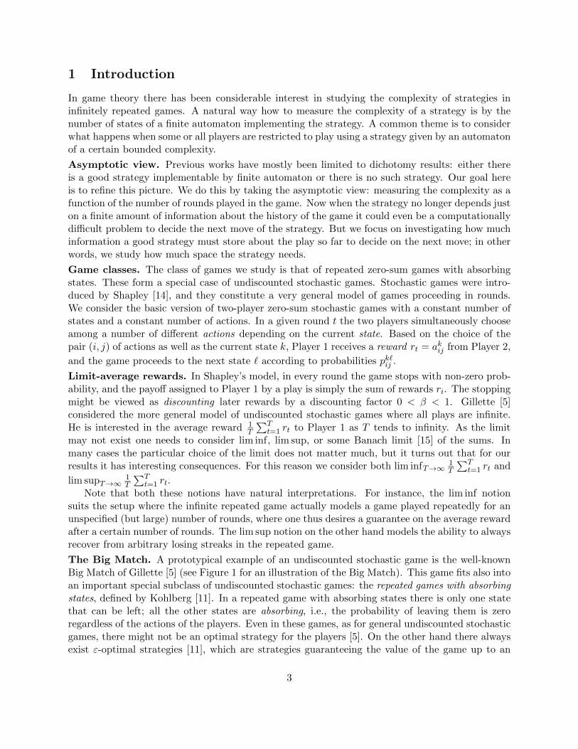
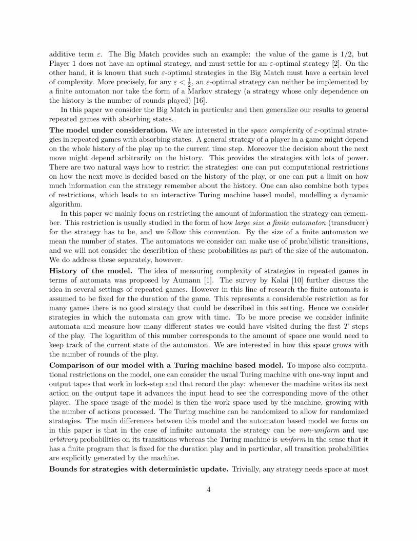
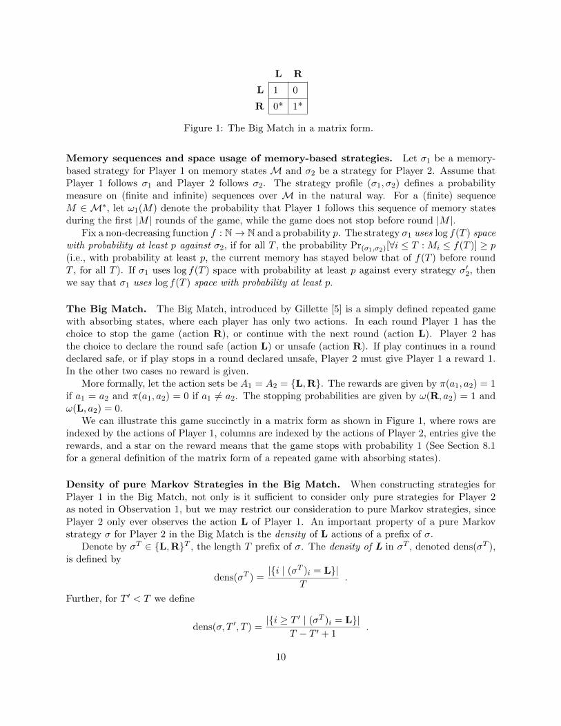
The Big Match. The Big Match, introduced by Gillette [5] is a simply defined repeated gamewith absorbing states, where each player has only two actions. In each round Player 1 has thechoice to stop the game (action R), or continue with the next round (action L). Player 2 hasthe choice to declare the round safe (action L) or unsafe (action R). If play continues in a rounddeclared safe, or if play stops in a round declared unsafe, Player 2 must give Player 1 a reward 1.In the other two cases no reward is given.

More formally, let the action sets be A1 = A2 = L,R. The rewards are given by π(a1, a2) = 1if a1 = a2 and π(a1, a2) = 0 if a1 6= a2. The stopping probabilities are given by ω(R, a2) = 1 andω(L, a2) = 0.

We can illustrate this game succinctly in a matrix form as shown in Figure 1, where rows areindexed by the actions of Player 1, columns are indexed by the actions of Player 2, entries give therewards, and a star on the reward means that the game stops with probability 1 (See Section 8.1for a general definition of the matrix form of a repeated game with absorbing states).

Density of pure Markov Strategies in the Big Match. When constructing strategies forPlayer 1 in the Big Match, not only is it sufficient to consider only pure strategies for Player 2as noted in Observation 1, but we may restrict our consideration to pure Markov strategies, sincePlayer 2 only ever observes the action L of Player 1. An important property of a pure Markovstrategy σ for Player 2 in the Big Match is the density of L actions of a prefix of σ.

Denote by σT ∈ L,RT , the length T prefix of σ. The density of L in σT , denoted dens(σT ),is defined by

dens(σT ) =|i | (σT )i = L|

T.

Further, for T ′ < T we define

dens(σ, T ′, T ) =|i ≥ T ′ | (σT )i = L|

T − T ′ + 1.

10

Observation 2. Suppose Player 2 follows a pure Markov strategy σ. Then for any play P andT < |P | we have

dens(σT ) =1

T

T∑T ′=1

rT ,

where rT is the reward given to Player 1 in round T . In particular, when P is infinite, we have

uinf(P ) = lim infT→∞

dens(σT ) ,

andusup(P ) = lim sup

T→∞dens(σT ) .

3 Small space ε-supremum-optimal strategies in the Big Match

For given ε > 0, let ξ = ε2. For any non-decreasing and unbounded function f : Z+ → Z+, we willnow give an ε-supremum optimal strategy σ∗1 for Player 1 in the Big Match that for all δ > 0 withprobability 1 − δ uses O(log f(T )) space. Let f be a strictly increasing unbounded function fromZ+ to R+, such that f(x) ≤ f(x) for all x ∈ Z+, and let F be the inverse of f . For simplicity,and without loss of generality, we assume that F (1) = 1 and F (T + 1) ≥ 2 · F (T ). Note that inparticular f(2 · T ) ≤ 2 · f(T ).

Intuitive description of the strategy and proof. The main idea for building the strategyis to partition the rounds of the game into epochs, such that epoch i has expected length F (i).The i’th epoch is further split into i sub-epochs. In each sub-epoch j of the i-th epoch we samplei2 rounds uniformly at random. In every round not sampled we simply stay in the same memorystate and play L with probability 1. We view the i2 samples as a stream of actions chosen byPlayer 2. We then follow a particular ξ-optimal base strategy σi,ξ1 for the Big Match on the samples

of sub-epoch j. This strategy σi,ξ1 is a suitably modified version of a strategy by Blackwell andFerguson [2] and Kohlberg [11].

More precisely, if σi,ξ1 stops in its k-th round when run on the samples of sub-epoch j, the strategyσ∗1 stops on the k-th sample in sub-epoch j. This will ensure that if σ∗1 stops with probability atleast

√ξ, the outcome is at least 1

2 − ξ.Also, for any 0 < δ < 1

2 and for sufficiently large i, depending on δ, if the samples have density

of L at most 12 − δ then σi,ξ1 stops on the samples with a positive probability depending only on ξ,

namely ξ4. For f(T ) = Θ(log T ), the division into sub-epochs ensures that if lim infT→∞ dens(σT ) <12 then infinitely many sub-epochs have density of L smaller than 1/2, and thus the play stops withprobability 1 in one of such epochs. This is not necessarily true for f(T ) smaller than log T .

The base strategy. The important inner part of our strategy is a ξ-optimal strategy σi,ξ1

parametrized by a non-negative integer i. These strategies are similar to ξ-optimal strategiesgiven by Blackwell and Ferguson [2] and Kohlberg [11] (in fact, setting i = 0 and replacing ξ4 byξ2 below one obtains the strategy used by Kohlberg).

11

The strategy σi,ξ1 uses deterministic updates of memory, and uses integers as memory states (wethink of the memory as an integer counter). The memory update function is given by

σi,u1 (a, j) =

j + 1 if a = L

j − 1 if a = R

and the action function is given by

σi,a1 (j)(R) =

ξ4(1− ξ)i+j if i+ j > 0

ξ4 if i+ j ≤ 0

The complete strategy We are now ready to define σ∗1. The memory states of this strategy are5-tuples (i, j, k, `, b) ∈ Z+ × Z+ × Z × N × 0, 1. Here i denotes the current epoch and j denotesthe current sub-epoch of epoch i. The number of samples already made in the current sub-epochis k. The memory state of the inner strategy is stored as `. Finally b is 1 if and only if the strategywill sample to the inner strategy in the next step.

The memory update function σ∗,u1 is as follows. Let (i, j, k, `, b) be the current memory stateand let a be the action of Player 2 in the current step. We then describe the distribution of thenext memory state (i′, j′, k′, `′, b′).

• The current step is not sampled if b = 0. In that case we keep i′ = i, j′ = j, k′ = k, and`′ = `.

• The current epoch is ending if j = i, k = i2 − 1, and b = 1. In that case i′ = i + 1, j′ = 1,k′ = 0, and `′ = 0.

• A sub-epoch is ending within the current epoch if j < i, k = i2 − 1, and b = 1. In that casei′ = i, j′ = j + 1, k′ = 0, and `′ = 0.

• We sample within a sub-epoch if k < i2 − 1 and b = 1. In that case i′ = i, j′ = j, k′ = k + 1,and `′ = σi,u1 (a, `).

Finally, in every case, we make a probabilistic choice whether to sample in the next step by letting

b′ = 1 with probability (i′)3

F (i′) .

The action function σ∗,a1 is given by

σ∗,a1 ((i, j, k, `, b))(a) =

σi,ξ1 (j)(a) if b = 1

1 if b = 0 and a = L

0 otherwise

.

In other words, if the current step is sampled, Player 1 follows the current base strategy, andotherwise always plays L.

The starting memory state is ms = (1, 1, 1, 0, 0). The states that can be reached in sub-epochj of epoch i are of the form (i, j, k, `, b) where 0 ≤ k < i2 and −i2 < ` < i2. Thus at most 4i4

states can be reached. The states are mapped to the natural numbers as follows: The memory(1, 1, 1, 0, 0) is mapped to 0 and for each epoch i, all states in epoch i are mapped to the numbers(in an arbitrary order) following the numbers mapped to by epoch i− 1.

12

Proof preliminaries It will be useful to consider the strategy modified to never stop. Thusdenote by σ1 the strategy for Player 1, where σu = σ∗,u1 and σa1(m)(L) = 1 for all memory statesm.

We next define random variables indicating the locations of the sample steps. Fix some strategyσ2 for Player 2. LetMσ1,σ2

ms be the memory sequence assigned to Player 1 when Player 1 follows σ1

and Player 2 follows σ2. For positive integers i, j, k let t(i, j, k) be the random variable indicatingthe round in which we sample the k’th time in sub-epoch j of epoch i. For simplicity of notationwe let t(i, 0, i2) denote t(i− 1, i− 1, (i− 1)2), and we let t(i, j) = t(i, j, 0) denote t(i, j − 1, i2).

3.1 Space usage of the strategy

We will here consider the space usage of σ∗1. First we will argue that with high probability, for alllarge enough i and any j, the length of sub-epoch j of epoch i, t(i, j, i2)− t(i, j − 1, i2), is close toF (i).

Lemma 7. For any γ, δ ∈ (0, 1/4), there is a constant M such that with probability at least 1− γ,for all i ≥M and all j ∈ 1, . . . , i, we have that

t(i, j, i2)− t(i, j − 1, i2) ∈ [(1− δ)F (i)/i, (1 + δ)F (i)/i] .

Proof. The expected number of times we sample during (1 − δ)F (i)/i steps of the i’th epoch is(1− δ)i2. If t(i, j, i2)− t(i, j − 1, i2) < (1− δ)F (i)/i then we sampled at least i2 times during these(1 − δ)F (i)/i steps of epoch i. This means that the actual number of samples is larger than itsexpectation by a factor δ/(1− δ). Thus by the multiplicative Chernoff bound, Theorem 45, we seethat,

Pr[t(i, j, i2)− t(i, j − 1, i2) < (1− δ)F (i)/i] < exp(−c(1− δ)i2

),

where c = ( δ1−δ )2/(2 + δ

1−δ ). Similarly, if t(i, j, i2)− t(i, j − 1, i2) > (1 + δ)F (i)/i then we sampled

less than i2 times during (1 + δ)F (i)/i steps which is less than the expected by a factor δ/(1 + δ)of its expectation. Again, by the multiplicative Chernoff bound,

Pr[t(i, j, i2)− t(i, j − 1, i2) > (1 + δ)F (i)/i] < exp

(−δ

2

2(1 + δ)i2

).

Thus for any M , we can bound from above the probability of any of the differences for i ≥M beingoutside of the required range by:

∞∑i=M

i ·(

exp(−c(1− δ)i2

)+ exp

(−δ

2

2(1 + δ)i2

)).

This sum is convergent so for sufficiently large M it can be bounded by γ. The lemma follows.

Now we bound the space usage of the strategy σ∗1.

Lemma 8. For all constants γ > 0, with probability at least 1 − γ, the space usage of σ∗1 isO(log f(T )).

13

Proof. Recall that there are at most 4 · i4 distinct possible memory states reachable during the j’thsub-epoch of epoch i, for all i, j. Thus, since there are i sub-epochs in epoch i there are at most4 · i5 distinct possible memory states reachable during the i’th epoch. It is then clear that there areat most

∑ir=0 4 · r5 ≤ 4 · i6 distinct possible memory states that can have been reached before the

end of epoch i, for all i. Because memory states in earlier epochs are mapped to smaller numbersthan latter epochs, we have that the strategy has not been in any state above that of 4 · i6 beforethe end of epoch i.

Fix some γ > 0. By Lemma 7, with probability at least 1 − γ, there is a M such that for alli ≥ M , the number t(i, i, i2) − t(i, 1, i2) is greater than F (i)

2 . Thus also t(i, i, i2) ≥ F (i)2 . Consider

any round T , for T ≥ t(M,M,M2). Let i be the epoch containing round T . By the preceding weknow that, before time step t(i + 1, i + 1, (i + 1)2) (which is greater than T ), the strategy have

only been in memory states below 4 · (i + 1)6. We also have that T ≥ t(i, i, i2) ≥ F (i)2 and hence

2f(T ) ≥ f(2T ) ≥ i, where the first inequality is by our assumption on F . Thus the strategy canonly have been in states below that of 4 · (2 · f(T ) + 1)6 before time step T . This is true for allsufficiently large T and thus the strategy uses at most O(log f(T )) space with probability 1−γ.

3.2 Play stopping implies good outcome

We first establish some properties of the base strategy σi,ξ1 . The proof of these uses ideas similar toproofs by Blackwell and Ferguson [2] and Kohlberg [11], where they showed ε-optimality of theirstrategies.

Lemma 9. Let T, i ≥ 1 be integers and 0 < ξ < 1 be a real number. Let σ ∈ L,RT be a arbitraryprefix of a pure Markov strategy for Player 2. Consider the first T rounds where the players playthe Big Match following σi,ξ1 and σ respectively. Let pwin be the probability that Player 1 stops thegame (i.e. plays R) and wins. Let ploss be the probability that Player 1 stops the game and loses.Then we have:

1.ploss ≤ (1− ξ)iξ3 + (1− ξ)−1pwin .

2. For any 0 < δ ≤ 12 and any T > i/(2δ), if dens(σ) ≤ 1

2 − δ then

pwin + ploss ≥ ξ4 .

Proof. Define d` = |`′ < ` | σ`′ = L| − |`′ < ` | σ`′ = R|. Note that d` is precisely the value of

the counter used by σi,ξ1 as memory in step `. For integer d, define

Kd = ` ∈ 1, . . . , T | (d` = d & σ` = L) or (d` = d+ 1 & σ` = R) .

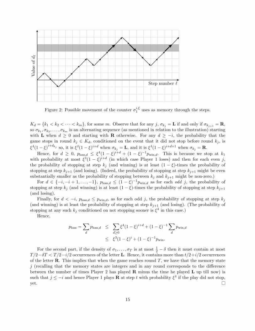
There is an illustration of how d` could evolve through the steps in Figure 2. The set Kd is thenthe times the counter moves between the pair of rows d and d + 1. Observe that the counter isalternately moving up and down in each Kd (for instance, in the gray row, the arrows are widerand first moves up, then down and then up again).

Notice that Kd partitions 1, . . . , T. Let ploss,d be the probability that the game stops at somestep ` ∈ Kd where σ` = L, and let pwin,d be the probability that the game stops at some step` ∈ Kd where σ` = R. We see that ploss is the sum of ploss,d, and that pwin is the sum of pwin,d. Let

14

Step number `

Valu

eofd`

Figure 2: Possible movement of the counter σi,ξ1 uses as memory through the steps.

Kd = k1 < k2 < · · · < km, for some m. Observe that for any j, σkj = L if and only if σkj+1= R,

so σk1 , σk2 , . . . , σkm is an alternating sequence (as mentioned in relation to the illustration) startingwith L when d ≥ 0 and starting with R otherwise. For any d ≥ −i, the probability that thegame stops in round kj ∈ Kd, conditioned on the event that it did not stop before round kj , is

ξ4(1− ξ)i+dkj so, it is ξ4(1− ξ)i+d when σkj = L, and it is ξ4(1− ξ)i+d+1 when σkj = R.

Hence, for d ≥ 0, ploss,d ≤ ξ4(1 − ξ)i+d + (1 − ξ)−1pwin,d. This is because we stop at k1

with probability at most ξ4(1 − ξ)i+d (in which case Player 1 loses) and then for each even j,the probability of stopping at step kj (and winning) is at least (1 − ξ)-times the probability ofstopping at step kj+1 (and losing). (Indeed, the probability of stopping at step kj+1 might be evensubstantially smaller as the probability of stopping between kj and kj+1 might be non-zero.)

For d ∈ −i,−i + 1, . . . ,−1, ploss,d ≤ (1 − ξ)−1pwin,d as for each odd j, the probability ofstopping at step kj (and winning) is at least (1− ξ)-times the probability of stopping at step kj+1

(and losing).Finally, for d < −i, ploss,d ≤ pwin,d, as for each odd j, the probability of stopping at step kj

(and winning) is at least the probability of stopping at step kj+1 (and losing). (The probability ofstopping at any such kj conditioned on not stopping sooner is ξ4 in this case.)

Hence,

ploss =∑d

ploss,d ≤∑d≥0

ξ4(1− ξ)i+d + (1− ξ)−1∑d

pwin,d

≤ ξ3(1− ξ)i + (1− ξ)−1pwin.

For the second part, if the density of σ1, . . . , σT is at most 12 − δ then it must contain at most

T/2−δT < T/2−i/2 occurrences of the letter L. Hence, it contains more than t/2+i/2 occurrencesof the letter R. This implies that when the game reaches round T , we have that the memory statej (recalling that the memory states are integers and in any round corresponds to the differencebetween the number of times Player 2 has played R minus the time he played L up till now) issuch that j ≤ −i and hence Player 1 plays R at step t with probability ξ4 if the play did not stop,yet.

15

We can now prove the main statement of this subsection, that if the probability of stopping isnot too small, Player 1 wins with probability close to 1/2 if play the stops.

Lemma 10. Let ξ ∈ (0, 1). Let σ be an pure Markov strategy for Player 2. If the probability thatplay stops is at least

√ξ, then we have that

Prσ∗1 ,σ[ Player 1 wins | play stops ] ≥ 1

2−√ξ .

Proof. We will in this proof continue playing in a state v, even if Player 1 plays R. Note that σ∗1can still generate a choice in this case. Let Ai,j be set of plays in which, between round 1 andround t(i, j, 1)− 1, Player 1 does not play R. Let Wi,j be the set of plays, in which, between roundt(i, j, 1) and round t(i, j, i2), Player 1 plays R and when he plays R for the first time between theserounds, Player 2 plays R as well. Similarly, let Li,j be the set of plays, in which, between roundt(i, j, 1) and round t(i, j, i2), Player 1 plays R and when he does so for the first time Player 2 playsL. Let S be the set of plays, in which Player 1 plays R in some round. Let W be the set ofplays, in which Player 1 plays R in some round and the first time he does so Player 2 also playsR. Let L be the set of plays, in which Player 1 plays R in some round and the first time he doesso Player 2 plays L. We see that S = W ∪ L. Clearly, Prσ

∗1 ,σ[W ] =

∑i,j Prσ

∗1 ,σ[Wi,j & Ai,j ] and

Prσ∗1 ,σ[L] =

∑i,j Prσ

∗1 ,σ[Li,j & Ai,j ].

Fix a possible value of all t(i, j, k)’s and denote by Y the event that these particular valuesactually occurs. Fix i and j. Conditioned on Y and Ai,j , between time t(i, j, 1) and t(i, j, i2)

Player 1 plays σi,ξ1 against a fixed strategy σt(i,j,1), σt(i,j,2), . . . , σt(i,j,i2) for Player 2. By Lemma 9,

the probability of losing such a game for Player 1 is at most ξ3(1 − ξ)i plus the probability ofwinning in this game divided by (1− ξ). Hence,

Pr[Li,j | Y,Ai,j ] ≤ ξ3(1− ξ)i + (1− ξ)−1 Pr[Wi,j | Y,Ai,j ].

Since the above inequality is true conditioned on arbitrary values of t(i, j1, j2)’s, it is true alsowithout the conditioning:

Pr[Li,j | Ai,j ] ≤ ξ3(1− ξ)i + (1− ξ)−1 Pr[Wi,j | Ai,j ].

Thus,

Prσ∗1 ,σ[L] =

∞∑i=1

i∑j=1

Pr[Li,j & Ai,j ]

=∞∑i=1

i∑j=1

Pr[Li,j | Ai,j ] · Pr[Ai,j ]

≤∞∑i=1

i∑j=1

(ξ3(1− ξ)i + (1− ξ)−1 Prσ

∗1 ,σ[Wi,j | Ai,j ]

)· Pr[Ai,j ]

≤∞∑i=1

i∑j=1

ξ3(1− ξ)i + (1− ξ)−1∞∑i=1

i∑j=1

Prσ∗1 ,σ[Wi,j & Ai,j ]

=

∞∑i=1

i · ξ3(1− ξ)i + (1− ξ)−1∞∑i=1

i∑j=1

Prσ∗1 ,σ[Wi,j & Ai,j ]

≤ ξ + (1− ξ)−1 Prσ∗1 ,σ[W ] .

16

Hence, (1−ξ) Prσ∗1 ,σ[L] ≤ ξ−ξ2 +Prσ

∗1 ,σ[W ], and so Prσ

∗1 ,σ[L]−Prσ

∗1 ,σ[W ] ≤ 2ξ. By our assumption

we also have that Prσ∗1 ,σ[L] + Prσ

∗1 ,σ[W ] = Prσ

∗1 ,σ[S] ≥

√ξ.

We want to find the minimum probability that we might win, conditioned on us stopping

Prσ∗1 ,σ[W | S] =

Prσ∗1 ,σ[W ]

Prσ∗1 ,σ[S]

=Prσ

∗1 ,σ[W ]

Prσ∗1 ,σ[W ] + Prσ

∗1 ,σ[L]

We see that it is greater than the solution of:

min xx+y

s.t. x+ y ≥√ξ

y − x ≤ 2ξ

Solving the above, we see that Prσ∗1 ,σ[W | S] ≥ 1

2 −√ξ and the lemma follows.

3.3 Low density means play stops

In this subsection we will prove that play will stop with probability 1 if the density of prefixes ofthe pure Markov strategy used by Player 2 is not infinitely often at least 1/2. First, we will showthat low density implies that some sequence of sub-epochs also have low density.

Lemma 11. Let δ ∈ (0, 1). Let σ be an arbitrary pure Markov strategy for Player 2. Let ai,j be somenumbers. Consider the event Y where t(i, j) = ai,j for all i, j. If lim supT→∞ dens(σT ) ≤ 1/2− δ,then conditioned on Y , there is an infinite sequence of sub-epochs and epochs (in, jn)n such thatdens(σ, ain,jn + 1, ain,(jn+1)) ≤ 1/2− δ/4.

Proof. Let M be such that for every T ′ ≥M we have that dens(σT′) ≤ 1/2− δ/2. Let (Tn)n be a

sequence such that T1 ≥M and for all n ≥ 1 we have that Tn+1 · δ/4 ≥ Tn and Tn = ai,j for somei, j. Let (i′n, j

′n)n be the sequence such that Tn = ai′n,j′n . This means that even if dens(σTn) = 0,

the density dens(σ, Tn + 1, Tn+1) is at most 1/2 − δ/4, because dens(σTn+1) ≤ 1/2 − δ/2. But,we then get that there exists some sub-epoch jn in epoch in, such that j′n ≤ jn ≤ j′n+1 and suchthat i′n ≤ in ≤ i′n+1 for which the density of that sub-epoch dens(σ, ain,jn + 1, ain,(jn+1)) is at most1/2 − δ/4, because not all sub-epochs can have density below that of the average sub-epoch. Butthen (in, jn)n satisfies the lemma statement.

We are now ready to prove the main statement of this subsection.

Lemma 12. Let σ be an arbitrary pure Markov strategy for Player 2. If

lim supT→∞

dens(σT ) < 1/2 ,

then when played against σ∗1 the play stops with probability 1.

Proof. Let δ > 0 be such that lim supT→∞ dens(σT ) ≤ 1/2 − δ. Consider arbitrary numbers ai,jand the event Y stating that t(i, j) = ai,j for all i, j. Let (in, jn)n be the sequence of sub-epochsand epochs shown to exists by Lemma 11 with probability 1. That is, for each (in, jn) we have thatsub-epoch jn of epoch in has density at most 1/2− δ/4. We see that, conditioned on Y that eachsample are sampled uniformly at random in each sub-epoch j of each epoch i, except for the lastsample. Now consider some fixed n. By Hoeffding’s inequality, Theorem 46 (setting ai = 0 and

17

bi = 1, and letting ci be i’th payoff for Player 1), the probability that in sub-epoch jn of epoch inthat among our i2n − 1 first samples we have δ

8 · ((in)2 − 1) additional L on top of the expectation(which is at most (1/2− δ/4) · ((in)2 − 1)) is bounded as

Pr

[dens(σt(in,jn,1), σt(in,jn,2), . . . , σt(in,jn,(in)2−1)) ≥

1

2− δ

8

]≤ 2 exp

(−

2( δ8((in)2 − 1))2

(in)2 − 1

)= 2 exp

(− δ

2

32((in)2 − 1)

).

For sufficiently large in, this is less than 12 . If on the other hand the number of L’s we sample is

less than (12 −

δ8)((in)2 − 1), we see that (in)2 − 1 > in/(16δ) for large enough in and in that case

we have, by Lemma 9, that we stop with probability at least ξ4 in sub-epoch jn of epoch in. Thus,for each of the infinitely many n’s for which in is sufficiently high, we have a probability of at leastξ4

2 of stopping. Thus play must stop with probability 1.The argument was conditioned on some fixed assignment of endpoints of sup-epochs and epochs,

but since there is such a assignment with probability 1 (since they are finite with probability 1),we conclude that the proof works without the condition.

3.4 Proof of main result

Theorem 13. The strategy σ∗1 is√ξ-supremum-optimal, and for all δ > 0, with probability at least

1− δ it uses space O(log f(T )).

Proof. The space usage follows from Lemma 8. Let s be the probability that the play stops. Wenow consider three cases, either (i) s = 1; or (ii)

√ξ < s < 1; or (iii) s ≤

√ξ. In case (i), if

s = 1, Player 1 wins with probability 12 −√ξ, by Lemma 10. In case (ii), if

√ξ < s < 1, then, by

Lemma 10, conditioned on the play stopping, Player 1 wins with probability Ws = 12 −√ξ and,

since s < 1, by Lemma 12 Ws = lim supT→∞ dens(σT ) ≥ 12 . Thus, Player 1 wins with probability

s ·Ws + (1− s) · Ws ≥ s · (1

2−√ξ) + (1− s)1

2≥ 1

2−√ξ

In case (iii), if s ≤√ξ, then by Lemma 12 Ws = lim supT→∞ dens(σT ) ≥ 1

2 . The winning probabilityis then at least

s · 0 + (1− s) · 1

2≥ 1−

√ξ

2≥ 1

2−√ξ

4 An ε-optimal strategy that uses log log T space for the Big Match

For given ε > 0, let ξ = ε2. In this section we give a ε-optimal strategy σ∗1 for Player 1 in the BigMatch that for all δ > 0 with probability 1− δ uses O(log log T ) space. The strategy is simply aninstantiation of the strategy σ∗1 from Section 3, setting f(T ) = dlog T e. We can then let f = log Tand F (T ) = 2T .

The claim about the space usage of σ∗1 is thus already established in Section 3. To obtain thestronger property of ε-optimality rather than just ε-supremum-optimality, we just need to establisha lim inf version of Lemma 12.

18

First we show a technical lemma. For a pure Markov strategy σ and a sequence of integersI = i1, i2, . . . , im, let σI be the sequence, σi1 , σi2 , . . . , σim . Note that σk = σ1,...,k.

Lemma 14. Let σ be a pure Markov strategy for Player 2, δ < 1/4 be a positive real, and M be apositive integer. Let lim infT→∞ dens(σT ) ≤ 1

2−δ. Let `1, `2, . . . be such that for all i ≥M , we havethat `i ∈ [(1− δ) · (2i+1 − 1), (1 + δ) · (2i+1 − 1)]. Then there exists a sequence k2, k3, . . . such thatfor infinitely many i > M , we have that `i−1 + δ2i−2 ≤ ki ≤ `i and dens(σ`i−1+1,...,ki) ≤

12 −

δ4 .

Proof. Let `i be as required. If there are infinitely many i such that dens(σ`i−1+1,...,`i) ≤12 −

δ4

then set ki = `i+1 and the lemma follows by observing (ki−`i−1) ≥ (1−δ)(2i+1−1)−(1+δ)(2i−1) =(1−3δ)2i ≥ δ2i−2, for i > M . So assume that only for finitely many i, dens(σ`i−1+1,...,`i) ≤

12 −

δ4 .

Thus the following claim can be applied for arbitrary large i0.

Claim 15. Let i0 ≥ M be given. If for every i ≥ i0, dens(σ`i−1+1,...,`i) >12 −

δ4 then there exist

j > i0 and k such that `j−1 + δ2j−2 ≤ k ≤ `j and dens(σ`j−1+1,...,k) ≤ 12 − δ.

We can use the claim to find k2, k3, . . . inductively. Start with large enough i0 ≥ M and setki = `i for all i ≤ i0. Then provided that we already inductively determined k2, k3, . . . , ki0 , weapply the above claim to obtain j and k, and we set kj = k and ki = `i, for all i = i0 + 1, . . . , j− 1.

So it suffices to prove the claim. For any d ≥ 1, `i0 · 2d−1 ≤ `i0+d and

dens(σ`i0+d) ≥(1

2 −δ4)(`i0+d − `i0)

`i0+d.

Furthermore, if d ≥ 1 + log(4/δ) then `i0 ≤ δ4`i0+d and

dens(σ`i0+d) ≥(

1

2− δ

4

)− δ

4=

1

2− δ

2.

Since lim infk→∞ dens(σk) ≤ 12 − δ, there must be k and d ≥ 1 + log(4/δ) such that `i0+d−1 ≤ k ≤

`i0+d and dens(σk) ≤ 12 − δ. Set j = i0 + d. Also

dens(σk) =dens(σ`j−1)`j−1 + dens(σ`j−1+1,...,k)(k − `j−1)

`j−1 + (k − `j−1),

which means(dens(σk)− dens(σ`j−1+1,...,k)

)(k − `j−1) =

(dens(σj−1)− dens(σk)

)`j−1

≥[(

1

2− δ

2

)−(

1

2− δ)]

`j−1 =δ

2`j−1 .

Thus dens(σ`j−1+1,...,k) ≤ dens(σk) which in turn is less than 12 − δ. Furthermore, k − `j−1 ≥

δ2`j−1 ≥ δ

2(1−δ)(2j−1) ≥ δ42j , provided that j ≥ 2. Hence, k and j have the desired properties.

We are now ready to prove the lim inf version of Lemma 12.

Lemma 16. Let σ be an arbitrary pure Markov strategy for Player 2. If

lim inft→∞

dens(σ1, . . . , σt) < 1/2 ,

then when played against σ∗1 the play stops with probability 1.

19

Proof. Let 0 < δ < 14 be such that

lim inft→∞

dens(σ1, . . . , σt) ≤ 1/2− δ

Pick arbitrary γ ∈ (0, 1). We will show that with probability at least 1 − γ the game stops, andthis implies the statement. Let M be given by Lemma 7 applied for γ and δ/2. Then we have thatwith probability at least 1− γ, for all i ≥M and j ∈ 1, . . . , i,

t(i, j, i2)− t(i, j − 1, i2) ∈ [(1− δ

2)2i/i, (1 +

δ

2)2i/i] .

Pick ti,j ∈ N, for i = 1, 2, . . . and j ∈ 1, . . . , i, so that ti,j−1 < ti,j where ti,0 stands forti−1,i−1. Let ti,j − ti,j−1 ∈ [(1 − δ

2)2i/i, (1 + δ2)2i/i], for all i ≥ M and j ∈ 1, . . . , i. Pick M ′

so that δ2(2M

′ − 1) ≥ maxtM,0, (1 − δ2)2M. Define `i = ti,i for all i ≥ 1. Then for all i ≥ M ′,

`i ∈ [(1− δ) · (2i+1 − 1), (1 + δ) · (2i+1 − 1)] as

`i = ti,i = tM,0 +∑

M≤i′≤i,1≤j≤i′ti′,j − ti′,j−1

≤ δ

2(2M

′ − 1) +∑

M≤i′≤ii′ · (1 +

δ

2)2i′/i′

≤ δ

2(2M

′ − 1) + (1 +δ

2) · (2i+1 − 1)

≤ (1 + δ) · (2i+1 − 1),

and similarly for the lower bound: `i ≥∑

i′,j ti′,j− ti′,j−1 ≥ (1− δ2)(2i+1−2M ) ≥ (1− δ) · (2i+1−1).

Thus Lemma 14 is applicable on `i with M set to M ′, and we obtain a sequence k2, k3, . . . suchthat dens(σ`i−1+1,...,ki) ≤ 1

2−δ4 and ki−`i−1 ≥ δ2i−2 for infinitely many i. Pick any of the infinitely

many i ≥ maxM ′, 32(1 + δ)/δ for which ki − `i−1 ≥ δ2i−2 and dens(σ`i−1+1,...,ki) ≤ 12 −

δ4 . Since

δ2i−3 ≥ (1 + δ)2i/i, there is some j ∈ 1, . . . , i such that `i−1 + δ2i−3 ≤ ki− (1 + δ)2i/i ≤ ti,j ≤ ki.Fix such j. Since ki ≤ ti,j + (1 + δ)2i/i, we have

dens(σ`i−1+1,...,ti,j ) =dens(σ`i−1+1,...,ki)(ki − `i−1)

ti,j + `i−1

≤dens(σ`i−1+1,...,ki)((1 + δ)2i/i+ ti,j − `i−1)

ti,j + `i−1

≤(

1

2− δ

4

)·(

1 +8(1 + δ)

i

)≤ 1

2− δ

4+

4(1 + δ)

i≤ 1

2− δ

8.

Hence, dens(σ`i−1+1,...,ti,j ) ≤ 12 −

δ8 . So for some j′ ∈ 1, . . . , j, dens(σti,j′−1+1,...,ti,j′ ) ≤

12 −

δ8 . We

can state the following claim.

Claim 17. For i large enough, conditioned on t(a, b, a2) = ta,b, for all a ≥ M and all b, andconditioned on that the game did not stop before the time ti,j′−1 + 1, the game stops during timesti,j′−1 + 1, . . . , ti,j′ with probability at least ξ4/2.

20

Conditioned on t(a, b, a2) = ta,b, for all a, b, the claim implies that the game stops with proba-bility 1. Note that the condition is true for some valid choice of ta,b with probability 1 − γ. Thisis because the claim can be invoked for infinitely many i’s and for each such i we will have ξ4/2chance of stopping.

It remains to prove the claim. Assume t(i, j′ − 1, i2) = ti,j′−1 and t(i, j′, i2) = ti,j′ . Clearly,

dens(σti,j′−1+1,...,ti,j′−1) ≤ dens(σti,j′−1+1,...,ti,j′ ) · (2i−1/(2i−1 − 1)) ≤ 1

2− δ

16,

for i large enough. So if we sample i2 − 1 times from σti,j′−1+1, . . . , σti,j′−1 we expect at most

(12 −

δ16)(i2− 1) of the letters to be L. By Hoeffding’s inequality, Theorem 46 (again setting ai = 0

and bi = 1, and letting ci be i’th payoff for Player 1), the probability that we get at least δ32(i2− 1)

additional L items on top of the expectation is given by

Pr

[dens(σt(i,j′,1), σt(i,j′,2), . . . , σt(i,j′,i2−1)) ≥

1

2− δ

32

]≤ 2 exp

(−

2( δ32(i2 − 1))2

i2 − 1

)= 2 exp

(− δ2

512(i2 − 1)

).

The probability is taken over the possible choices of t(i, j′, 1) < t(i, j′, 2) < · · · < t(i, j′, i2 − 1)assuming t(i, j′ − 1, i2) = ti,j′−1 and t(i, j′, i2) = ti,j′ . For i sufficiently large, 2e−δ

2(i2−1)/512 ≤ 1/2.Whenever

dens(σt(i,j′,1), σt(i,j′,2), . . . , σt(i,j′,i2−1)) ≤1

2− δ

32

we have at least ξ4 chance of stopping by Lemma 9, as Player 1 plays σi+j′,ξ

1 against

σt(i,j′,1), σt(i,j′,2), . . . , σt(i,j′,i2−1)

and i2 − 1 > i/δ ≥ (i + j′)/2δ for sufficiently large i. Hence, the game stops with probability atleast (1− 1/2) · ξ4 = ξ4/2. The claim, and thus the lemma, follows.

We can now conclude with the main result of this section.

Theorem 18. The strategy σ∗1 is√ξ-optimal, and for all δ > 0, with probability at least 1 − δ it

uses space O(log log T ).

Proof. This is proved just like Theorem 13, except that Lemma 16 is used in place of Lemma 12.

We can also improve the strategy and get the following corollary.

Corollary 19. For any natural number k, there is a strategy which is 2−k-optimal, has patience 2and can be implemented on a Turing machine, using at most 1 random bit and amortized constanttime1 per round and with probability at least 1− δ does it use tape space O(log log(T ) + log k) uptoround T .

1i.e. for all T , let c(T ) be the computation used for the first T rounds, then c(T )T

is some constant

21

Proof. We will only sketch the necessary ingredients for the proof. We will modify the strategy σ∗1as defined in Section 4 to use less patience. First, it is easy to see that the probability that twosample points are ever within a polynomial in i distance of each other is small, in any sufficientlyhigh epoch i, and thus we can ignore this event. The idea is as follows: Each sub-epoch of epoch iis split into blocks of length B = iO(1) ·k (where we simply keep track of the current location withinthe current block, but not the current block number). The purpose of each block is to provide allthe randomness needed for the next block. Hence, it needs to (1) decide if there is a sample pointin the next block; and (2) if so where; and (3) if we should stop on that sample point. Observe thatwe are ignoring the possibility that there are more than 1 sample point in a block. It is easy to seethat the number of random bits needed in total to generate all those events is less than iO(1) · kand thus it can be done with at most 1 random bit per round, implying the patience bound. Toget the tape space bound, we utilize the three following simple ideas:

Idea 1: To get a probability like∏aj , for some sequence of probabilities aj of length `, one can test

if sub-events that happens with probability ai for all i all happens. This requires only spacefor a counter counting up to ` and space for the event that uses the most space (by reusingthe space for the event).

Idea 2: To get an probability like 2−x (or similarly 1 − 2−x) one can simply flip x coins and if allcomes up tails, then the event happens. This requires only space for a counter counting upto x.

Idea 3: To get an probability like y2x , for any natural number x and y, one can simply use x random

bits. This uses x many bits of space.

Direct application of these three ideas suffice to get all three events in O(log i + log k) many bits.Observe that we can do this easily on a two tape Turing machine (one is used for events followingidea 3 and one for the constant number of counters) and we only need amortized constant time ineach round (to increment and/or reset some subset of the counters on the first tape and perhapsto add one more random bit or reset the second tape).

5 Lower bound on patience

When considering a strategy of a player one may want to look at how small or large the probabilitiesoccurring in that strategy are. The parameter of interest is the patience of the strategy which is thereciprocal of the smallest non-zero probability occurring in the strategy. Patience is closely relatedto the expected length of finite plays as small probability events will not occur if the play is tooshort so they will have little influence on the overall outcome [11, 6]. Care has to be taken how todefine patience for strategies with infinitely many possible events. One thing to note of our spaceefficient strategies is that the patience of the states in which we are with high probability duringthe first T steps is approximately T , for rounds T close to the end of an epoch. In this section weshow that this is essentially necessary. So if the space used by the strategy with high probabilityis log f(T ), then the first f(T ) states must have patience about T . Thus the smaller the space thestrategy uses the larger the patience the states must have.

The main theorem of this section states that if the patience of the f(T ) states in which Player1 is with high probability is less than about T 1/f(T ) then the strategy is bad for Player 1. It is easyto observe that events with probability substantially less than 1/T are unlikely to occur during the

22

first T steps of the game so one should expect the patience of a good strategy for Player 1 to be inthe range between roughly T 1/f(T ) and T .

One may wonder whether the exponent 1/f(T ) in T 1/f(T ) is necessary. It turns out that it is,so our lower bound is close to optimal using a technique like in Corollary 19.

We use the following definitions to deal with the fact that our strategies use infinitely manytransitions so their overall patience is infinite.

For a memory based strategy σ1 of Player 1 in a repeated zero-sum game with absorbing states,the patience of a set of memory states M is defined as:

pat(M) = max

1

σa1(m)(a1),

1

σu1 (a1, a2,m)(m′), m,m′ ∈M,a1 ∈ A1, a2 ∈ A2

.

The patience of the other player is defined similarly.

Theorem 20. Let δ, ε > 0 be reals and f : N → N be an unbounded non-decreasing function suchthat f(T ) ≤ 1

4 log1/ε T for all large enough T . If a strategy σ1 of Player 1 uses space log f(T ) beforetime T with probability at least 1 − δ, and the patience of the set of lexicographically first f(T )memory states is at most T 1/(2f(T )) for all T large enough, then there is a strategy σ2 of Player 2such that u(sup, (σ1, σ2)) ≤ δ + 2ε.

Proof. Assume that ε < 1/2 and pick an integer k sufficiently large. For i > 0, define `i = ε−i andTi =

∑ij=1 `j . The strategy σ2 of Player 2 proceeds in phases, each phase i is of length `i. In the

first k phases, Player 2 plays L with probability 1 − ε and R with probability ε. In each phasei > k, Player 2 plays R for the first (1 − ε)`i steps, and afterwards he plays L with probability1− ε and R with probability ε. Notice, if the game does not stop by Player 1 playing R at somepoint then the expected lim sup payoff to Player 1 is at most ε.

Our goal is to show that if the game stops then the expected payoff to Player 1 is at mostδ+ 2ε. If the game stops during the last ε`i steps of a phase i, then the expected payoff to Player 1is ε as the probability of Player 2 playing R at that time is ε. If the game stops during the first(1 − ε)`i steps of a phase i > k, then the payoff of Player 1 is 1. Our goal is to argue that theoverall probability that Player 1 stops during the first (1− ε)`i steps of some phase i > k is small.

For any t > 0, denote by M(t) the set of the lexicographically first f(t) memory states (i.e.those mapped to a number below f(t). Let C be the event that for all steps t, Player 1 is in oneof the states in M(t). For t < t′, let S(t, t′) be the event that Player 1 plays R in one of the steps[t, t′). Let Ai(t) be the event that at time t, Player 1 is in one of the states in M(Ti) and there issome memory state in M(Ti) that can be reached from the state current at time t and in whichthere is a non-zero probability of playing R (i.e., stopping).

The probability that C does not occur is at most δ so for the rest of the proof we will assumethat C occurs. Let k be large enough, and i > k. It is clear that if S(Ti−1, Ti−1 + (1− ε)`i) occursthen Ai(Ti−1) must have occurred as well so:

Pr[S(Ti−1, Ti−1 + (1− ε)`i)] ≤ Pr[Ai(Ti−1)] .

Furthermore, if Ai(Ti−1) occurs then Ai(t) occurs for all t < Ti−1. For t ∈ [Ti−1−ε`i−1, Ti−1−f(Ti)),if Ai(t) occurs then within the next f(Ti) steps the strategy of Player 1 might reach a state in whichPlayer 1 chooses the stopping action R with non-zero probability. Because of the patience of M(Ti)

23

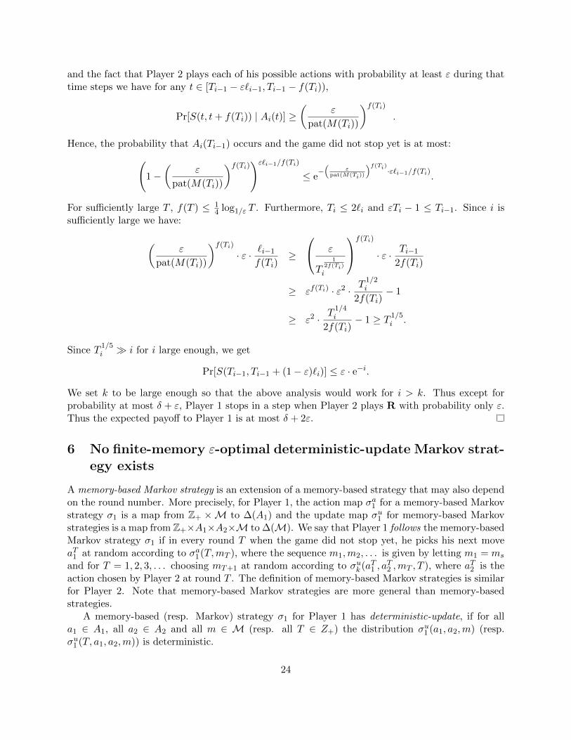
and the fact that Player 2 plays each of his possible actions with probability at least ε during thattime steps we have for any t ∈ [Ti−1 − ε`i−1, Ti−1 − f(Ti)),

Pr[S(t, t+ f(Ti)) | Ai(t)] ≥(

ε

pat(M(Ti))

)f(Ti)

.

Hence, the probability that Ai(Ti−1) occurs and the game did not stop yet is at most:(1−

(ε

pat(M(Ti))

)f(Ti))ε`i−1/f(Ti)

≤ e−(

εpat(M(Ti))

)f(Ti)·ε`i−1/f(Ti).

For sufficiently large T , f(T ) ≤ 14 log1/ε T . Furthermore, Ti ≤ 2`i and εTi − 1 ≤ Ti−1. Since i is

sufficiently large we have:

(ε

pat(M(Ti))

)f(Ti)

· ε · `i−1

f(Ti)≥

ε

T1

2f(Ti)

i

f(Ti)

· ε · Ti−1

2f(Ti)

≥ εf(Ti) · ε2 ·T

1/2i

2f(Ti)− 1

≥ ε2 ·T

1/4i

2f(Ti)− 1 ≥ T 1/5

i .

Since T1/5i i for i large enough, we get

Pr[S(Ti−1, Ti−1 + (1− ε)`i)] ≤ ε · e−i.

We set k to be large enough so that the above analysis would work for i > k. Thus except forprobability at most δ + ε, Player 1 stops in a step when Player 2 plays R with probability only ε.Thus the expected payoff to Player 1 is at most δ + 2ε.

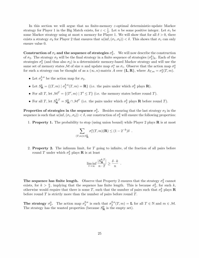
6 No finite-memory ε-optimal deterministic-update Markov strat-egy exists

A memory-based Markov strategy is an extension of a memory-based strategy that may also dependon the round number. More precisely, for Player 1, the action map σa1 for a memory-based Markovstrategy σ1 is a map from Z+ ×M to ∆(A1) and the update map σu1 for memory-based Markovstrategies is a map from Z+×A1×A2×M to ∆(M). We say that Player 1 follows the memory-basedMarkov strategy σ1 if in every round T when the game did not stop yet, he picks his next moveaT1 at random according to σa1(T,mT ), where the sequence m1,m2, . . . is given by letting m1 = ms

and for T = 1, 2, 3, . . . choosing mT+1 at random according to σuk (aT1 , aT2 ,mT , T ), where aT2 is the

action chosen by Player 2 at round T . The definition of memory-based Markov strategies is similarfor Player 2. Note that memory-based Markov strategies are more general than memory-basedstrategies.

A memory-based (resp. Markov) strategy σ1 for Player 1 has deterministic-update, if for alla1 ∈ A1, all a2 ∈ A2 and all m ∈ M (resp. all T ∈ Z+) the distribution σu1 (a1, a2,m) (resp.σu1 (T, a1, a2,m)) is deterministic.

24

In this section we will argue that no finite-memory ε-optimal deterministic-update Markovstrategy for Player 1 in the Big Match exists, for ε < 1

2 . Let n be some positive integer. Let σ1 besome Markov strategy using at most n memory for Player 1. We will show that for all δ > 0, thereexists a strategy σ2 for Player 2 that ensures that u(inf, (σ1, σ2)) < δ. This shows that σ1 can onlyensure value 0.

Construction of σ2 and the sequence of strategies σk2 . We will now describe the constructionof σ2. The strategy σ2 will be the final strategy in a finite sequence of strategies (σk2 )k. Each of thestrategies σk2 (and thus also σ2) is a deterministic memory-based Markov strategy and will use thesame set of memory statesM of size n and update map σu1 as σ1. Observe that the action map σa2for such a strategy can be thought of as a (∞, n)-matrix A over L,R, where AT,m = σa2(T,m).

• Let σk,a2 be the action map for σ2.

• Let SkR = (T,m) | σk,a2 (T,m) = R (i.e. the pairs under which σk2 plays R).

• For all T , let MT = (T ′,m) | T ′ ≤ T (i.e. the memory states before round T ).

• For all T , let Sk,TR = SkR ∩MT (i.e. the pairs under which σk2 plays R before round T ).

Properties of strategies in the sequence σk2 . Besides ensuring that the last strategy σ2 in thesequence is such that u(inf, (σ1, σ2)) < δ, our construction of σk2 will ensure the following properties:

1. Property 1. The probability to stop (using union bound) while Player 2 plays R is at most∑(T,m)∈Sk

R

σa1(T,m)(R) ≤ (1− 2−k)δ .

2. Property 2. The infimum limit, for T going to infinite, of the fraction of all pairs beforeround T under which σk2 plays R is at least

lim inft→∞

|Sk,TR |n · T

≥ δ · kn

.

The sequence has finite length. Observe that Property 2 ensures that the strategy σk2 cannotexists, for k > n

δ , implying that the sequence has finite length. This is because σk2 , for such k,otherwise would require that there is some T , such that the number of pairs such that σk2 plays Rbefore round T is strictly more than the number of pairs before round T .

The strategy σ02. The action map σ0,a

2 is such that σ0,a2 (T,m) = L for all T ∈ N and m ∈ M.

The strategy has the wanted properties (because S0R is the empty set).

25

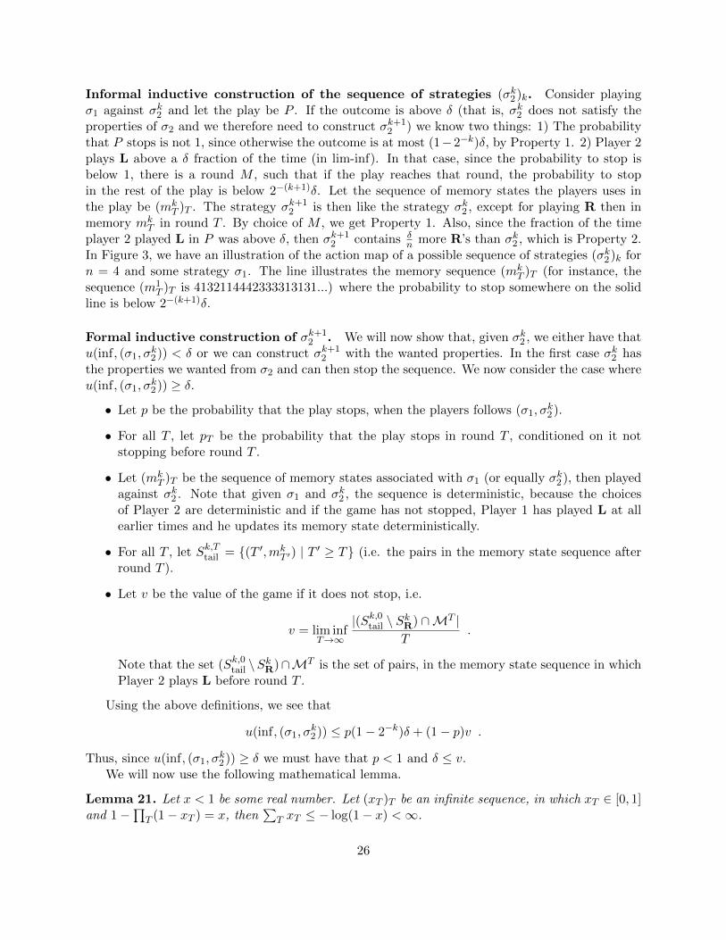
Informal inductive construction of the sequence of strategies (σk2 )k. Consider playingσ1 against σk2 and let the play be P . If the outcome is above δ (that is, σk2 does not satisfy theproperties of σ2 and we therefore need to construct σk+1

2 ) we know two things: 1) The probabilitythat P stops is not 1, since otherwise the outcome is at most (1−2−k)δ, by Property 1. 2) Player 2plays L above a δ fraction of the time (in lim-inf). In that case, since the probability to stop isbelow 1, there is a round M , such that if the play reaches that round, the probability to stopin the rest of the play is below 2−(k+1)δ. Let the sequence of memory states the players uses inthe play be (mk

T )T . The strategy σk+12 is then like the strategy σk2 , except for playing R then in

memory mkT in round T . By choice of M , we get Property 1. Also, since the fraction of the time

player 2 played L in P was above δ, then σk+12 contains δ

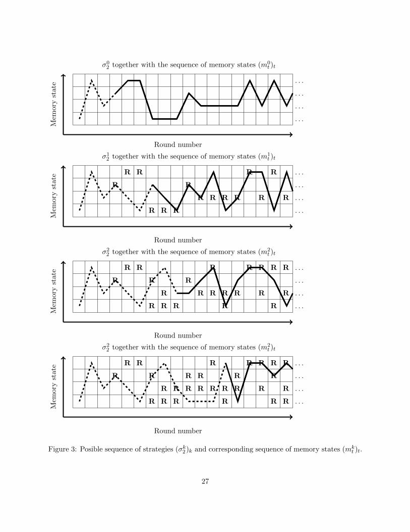
n more R’s than σk2 , which is Property 2.In Figure 3, we have an illustration of the action map of a possible sequence of strategies (σk2 )k forn = 4 and some strategy σ1. The line illustrates the memory sequence (mk

T )T (for instance, thesequence (m1

T )T is 4132114442333313131...) where the probability to stop somewhere on the solidline is below 2−(k+1)δ.

Formal inductive construction of σk+12 . We will now show that, given σk2 , we either have that

u(inf, (σ1, σk2 )) < δ or we can construct σk+1

2 with the wanted properties. In the first case σk2 hasthe properties we wanted from σ2 and can then stop the sequence. We now consider the case whereu(inf, (σ1, σ

k2 )) ≥ δ.

• Let p be the probability that the play stops, when the players follows (σ1, σk2 ).

• For all T , let pT be the probability that the play stops in round T , conditioned on it notstopping before round T .

• Let (mkT )T be the sequence of memory states associated with σ1 (or equally σk2 ), then played

against σk2 . Note that given σ1 and σk2 , the sequence is deterministic, because the choicesof Player 2 are deterministic and if the game has not stopped, Player 1 has played L at allearlier times and he updates its memory state deterministically.

• For all T , let Sk,Ttail = (T ′,mkT ′) | T ′ ≥ T (i.e. the pairs in the memory state sequence after

round T ).

• Let v be the value of the game if it does not stop, i.e.

v = lim infT→∞

|(Sk,0tail \ SkR) ∩MT |T

.

Note that the set (Sk,0tail \SkR)∩MT is the set of pairs, in the memory state sequence in which

Player 2 plays L before round T .

Using the above definitions, we see that

u(inf, (σ1, σk2 )) ≤ p(1− 2−k)δ + (1− p)v .

Thus, since u(inf, (σ1, σk2 )) ≥ δ we must have that p < 1 and δ ≤ v.

We will now use the following mathematical lemma.

Lemma 21. Let x < 1 be some real number. Let (xT )T be an infinite sequence, in which xT ∈ [0, 1]and 1−

∏T (1− xT ) = x, then

∑T xT ≤ − log(1− x) <∞.

26

. . .

. . .

. . .

. . .

σ02 together with the sequence of memory states (m0

t )t

Mem

ory

stat

e

Round number

R R R R . . .

R R . . .

R R R R R R . . .

R R R . . .

σ12 together with the sequence of memory states (m1

t )t

Mem

ory

stat

e

Round number

R R R R R R R . . .

R R R . . .

R R R R R R R . . .

R R R R R . . .

σ22 together with the sequence of memory states (m2

t )t

Mem

ory

stat

e

Round number

R R R R R R R . . .

R R R R R R . . .

R R R R R R R R R . . .

R R R R R R . . .

σ22 together with the sequence of memory states (m2

t )t

Mem

ory

stat

e

Round number

Figure 3: Posible sequence of strategies (σk2 )k and corresponding sequence of memory states (mkt )t.

27

Proof. We have that all xT < 1, since otherwise the product would be 0, and hence x = 1. Also,we get that ∏

T

(1− xT ) = 1− x⇒∑T

log(1− xT ) = log(1− x)

⇒ −∑T

log(1− xT ) = − log(1− x)⇒∑T

xT ≤ − log(1− x) .

The last inequality comes from that f(y) = − log(1 − y) ≥ y for y ∈ [0, 1). This follows fromf(0) = 0 and f ′(y) = 1

1−y ≥ 1, for y ∈ [0, 1).

We have that 1−∏T (1− pT ) = p and by Lemma 21 we then get that

∑T pT is finite. Hence,

there exists some M such that∑∞

T=M pT ≤ δ2k+1 .

We can now define σk+1,a2 . Let

σk+1,a2 (T,m) =

R if (T,m) ∈ Sk,Mtail

σk,a2 (T,m) otherwise

The strategy σk+12 satisfies the wanted properties. We will now show that σk+1

2 satisfiesthe wanted properties.

1. That Property 1 is satisfied comes from that∑(T,m)∈Sk+1

R

σa1(T,m)(R) ≤∑

(T,m)∈SkR

σa1(T,m)(R) +∑

(T,m)∈Sk,Mtail

σa1(T,m)(R)

≤ (1− 2−k)δ + 2−k−1δ = (1− 2−k−1)δ .

2. That Property 2 is satisfied can be seen as follows. We have that

lim infT→∞

|Sk+1,TR |n · T

= lim infT→∞

|Sk,TR |+ |(Sk,Mtail \ S

kR) ∩MT |

n · T

≥ lim infT→∞

|Sk,TR |n · T

+ lim infT→∞

|(Sk,Mtail \ SkR) ∩MT |

n · T.

Since the properties are satisfied for σk2 , we get that lim infT→∞|Sk,T

R |n·T ≥ δk

n . We thus justneed to argue that

lim infT→∞

|(Sk,Mtail \ SkR) ∩MT |

n′ · T≥ δ

n

and we are done. That statement can be seen as follows

δ ≤ v ⇒ δ ≤ lim infT→∞

|(Sk,0tail \ SkR) ∩MT |T

⇒ δ

n≤ lim inf

T→∞

|(Sk,0tail \ SkR) ∩MT |

n′ · T⇒

δ

n≤ lim inf

T→∞

|(Sk,Mtail \ SkR) ∩MT |

n · T,

where the last inequality comes from that Sk,0tail consists of the same pairs as Sk,Mtail and thenM more.

28

The above leads to the following theorem.

Theorem 22. For all ε < 12 , there exists no finite-memory deterministic-update ε-optimal Markov

strategy for Player 1 in the Big Match.

7 Generalized Big Match Games

In order to generalize our results to arbitrary repeated games with absorbing states, we follow theapproach of Kohlberg and consider first the subset of such games where Player 1, like in the BigMatch, has just the choice whether to declare that the game should stop or continue. But unlikethe Big Match, in case Player 1 declares the game should stop, the game will only stop with somenon-zero probability (that depends on the action of Player 2). Furthermore, Player 2 can have anynumber of actions and the rewards can be arbitrary. We call such games generalized Big Matchgames.

More formally, a generalized Big Match game G is specified as follows. Let A1 = L,R andlet A2 be any finite set. The rewards π(a1, a2) are arbitrary, but the stop probabilities ω(a1, a2)must satisfy that ω(L, a2) = 0 and ω(R, a2) > 0 for all a2 ∈ A2.

Our strategies for generalized Big Match games will follow the same template as those givenin Sections 3 and 4. The change required is a modification of the base strategies σi,ξ1 . The proof

that these new base strategies τ i,ξ1 have the desired properties follow those for σi,ξ1 , but uses alsoadditional ideas similar to those of Kohlberg[11].

Given G we define the derived matrix game G by

Ga1,a2 =

π(a1, a2) if a1 = L

ω(a1, a2) · π(a1, a2) if a1 = R.

Assumption 1. In the remainder of this section we make the following assumptions about thegiven generalized Big Match game G:

• The entries of G are integer.

• The value G is 0.

• Player 1 does not have a pure optimal strategy in G.

We observe that the last requirement means that in the matrix game G Player 1 has a uniqueoptimal strategy and it plays each action with non-zero probability.

Define ω = mina2 ω(R, a2) to be the minimum non-zero stop probability of G and K =maxa1,a2 |Ga1,a2 | be the maximum magnitude of an entry of G.

Remark. As noted in Observation 1, it is sufficient to consider only pure strategies for Player 2.Unlike for the Big Match, here play may continue even when Player 1 chooses the action R, andhence it is not sufficient to consider only pure Markov strategies for Player 2. We shall however(as done also by Kohlberg) give only the proof for this special case and just note that the proof forgeneral pure strategies of Player 2 is done along the same lines

29

Generalized density of pure Markov strategies In order to generalize our strategies givenin Sections 3 and 4, we must first generalize the notion of density of a pure Markov strategy σ forPlayer 2. We then define

gdens(σT ) =

∑Ti=1 π(L, σi)

T,

and further, for T ′ < T we define

gdens(σ, T ′, T ) =

∑Ti=T ′ π(L, σi)

T − T ′.

We can make a similar correspondence between the generalized density of a play and the averageof the rewards received by Player 1. The main difference here is that the play may possibly continuewhenever Player 1 plays the action R. However, the event that Player 1 plays action R an infinitenumber of times happens with probability 0, since each time Player 1 does play action R, the gamestops with probability at least ω > 0 by definition.

Observation 3. Suppose Player 2 follows a pure Markov strategy σ. Consider a play P in whichPlayer 1 plays only the action L. Then for any T < |P | we have

gdens(σT ) =1

T

T∑T ′=1

rT ,

where rT is the reward given to Player 1 in round T . Consider now an infinite play P in whichPlayer 1 plays action R only a finite number of times. Then we have

uinf(P ) = lim infT→∞

gdens(σT ) ,

andusup(P ) = lim sup

T→∞gdens(σT ) .

We need the following simple statement, which can be viewed as a quantified version of [11,Lemma 2.5].

Lemma 23. Let σ be a pure Markov strategy for Player 2, and let j be any integer. If T ·gdens(σT ) ≤ −j · 2K then

T∑i=1

ω(R, σTi ) · π(R, σTi ) ≥ j .

Proof. Let σ1 be the (unique) optimal strategy in G. By Assumption 1 we have that σ1(L) > 0and that the value of G is 0. This immediately implies that σ1(L) > 1/2K, since p = σ1(L) mustsatisfy an equation of the form

p · GL,a2 + (1− p) · GR,a2 = 0 ,

for some a2 ∈ A2, where the entries GL,a2 and GR,a2 are non-zero and integers of magnitude atmost K.

30

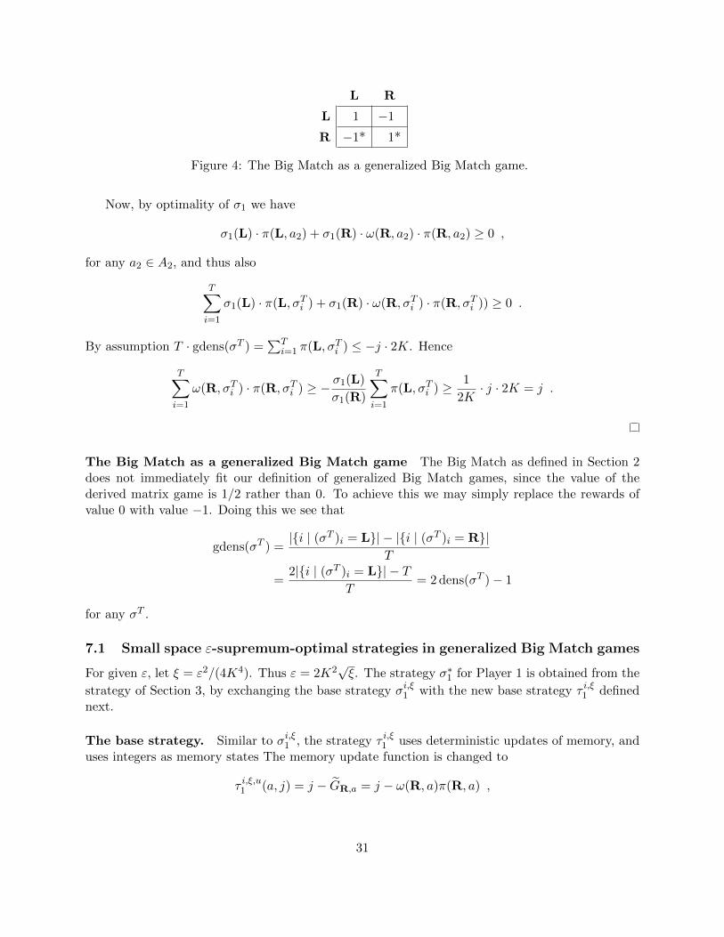
L R

L 1 −1

R −1* 1*

Figure 4: The Big Match as a generalized Big Match game.

Now, by optimality of σ1 we have

σ1(L) · π(L, a2) + σ1(R) · ω(R, a2) · π(R, a2) ≥ 0 ,

for any a2 ∈ A2, and thus also

T∑i=1

σ1(L) · π(L, σTi ) + σ1(R) · ω(R, σTi ) · π(R, σTi )) ≥ 0 .

By assumption T · gdens(σT ) =∑T

i=1 π(L, σTi ) ≤ −j · 2K. Hence

T∑i=1

ω(R, σTi ) · π(R, σTi ) ≥ − σ1(L)

σ1(R)

T∑i=1

π(L, σTi ) ≥ 1

2K· j · 2K = j .

The Big Match as a generalized Big Match game The Big Match as defined in Section 2does not immediately fit our definition of generalized Big Match games, since the value of thederived matrix game is 1/2 rather than 0. To achieve this we may simply replace the rewards ofvalue 0 with value −1. Doing this we see that

gdens(σT ) =|i | (σT )i = L| − |i | (σT )i = R|

T

=2|i | (σT )i = L| − T

T= 2 dens(σT )− 1

for any σT .

7.1 Small space ε-supremum-optimal strategies in generalized Big Match games

For given ε, let ξ = ε2/(4K4). Thus ε = 2K2√ξ. The strategy σ∗1 for Player 1 is obtained from the

strategy of Section 3, by exchanging the base strategy σi,ξ1 with the new base strategy τ i,ξ1 definednext.

The base strategy. Similar to σi,ξ1 , the strategy τ i,ξ1 uses deterministic updates of memory, anduses integers as memory states The memory update function is changed to

τ i,ξ,u1 (a, j) = j − GR,a = j − ω(R, a)π(R, a) ,

31

whereas the action function is unchanged as

τ i,ξ,a1 (j)(R) =

ξ4(1− ξ)i+j if i+ j > 0

ξ4 if i+ j ≤ 0.

Note that when the Big Match is redefined as a generalized Big Match game, we have that τ i,ξ1 = σi,ξ1 .We will next generalize the statements of Section 3 in the following paragraphs.

7.1.1 Space usage of the strategy

We will here consider the space usage of σ∗1. Like for the strategy σ∗1 for the Big Match we areinterested in the length of the epochs and can generalize Lemma 7 to generalized Big Match.

Lemma 24. For any γ, δ ∈ (0, 1/4), there is a constant M such that with probability at least 1−γ,for all i ≥M and all j ∈ 1, . . . , i, we have that

t(i, j, i2)− t(i, j − 1, i2) ∈ [(1− δ)F (i)/i, (1 + δ)F (i)/i] .

Proof. The proof is precisely the same as for Lemma 7, since it only concerns itself with the lengthof epochs and not with the base strategy, and only the base strategy has changed as compared tosection Section 3.

We next give a generalization of Lemma 8.

Lemma 25. For all constants γ > 0, with probability at least 1 − γ, the space usage of σ∗1 isO(log f(T ) + logK).

Proof. Observe that the base strategy τ i,ξ1 can reach a factor of 2K more memory states upto round

T than σi,ξ1 , since σi,ξ1 changes its counter by ±1 in each round while τ i,ξ1 changes its counter bysome number in −K, . . . ,K. Thus, σ∗1 uses at most a factor 2K more memory states then using

τ i,ξ1 as the base strategy instead of σi,ξ1 in round T for any T . The statement then follows from asimilar proof as the one for Lemma 8.

7.1.2 Play stopping implies good outcome

Lemma 26. Let T, i ≥ 1 be integers and 0 < ξ < 1 be a real number. Let σ ∈ (A2)T be an arbitraryprefix of a pure Markov strategy for Player 2. Consider the first T rounds where the players playG following τ i,ε1 and σ respectively.

Let S ∈ 1, . . . , T ∪ ∞ be a random variable in case the game stops in the first T roundsdenotes that round, and is ∞ otherwise. Let U be the random variable that denotes the outcome incase the game stops in the first T rounds, and is 0 otherwise. Then

1.−E[U | U < 0] Pr[U < 0] ≤ ξ3(1− ξ)i−K+1 + (1− ξ)1−2KE[U | U > 0] Pr[U > 0] .

2. If gdens(σT ) ≤ −i · 2K/T thenPr[S <∞] ≥ ξ4 · ω .

32

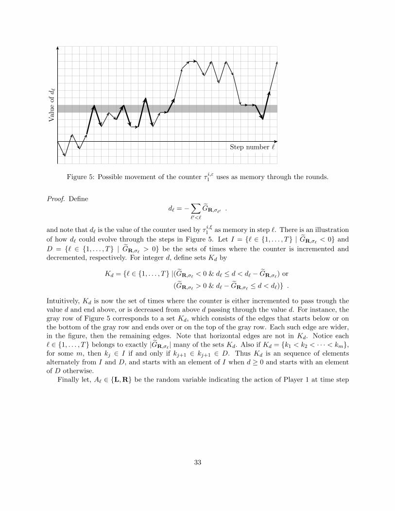
Step number `

Valu

eofd`

Figure 5: Possible movement of the counter τ i,ε1 uses as memory through the rounds.

Proof. Define

d` = −∑`′<`

GR,σ`′ .

and note that d` is the value of the counter used by τ i,ξ1 as memory in step `. There is an illustration

of how d` could evolve through the steps in Figure 5. Let I = ` ∈ 1, . . . , T | GR,σ` < 0 and

D = ` ∈ 1, . . . , T | GR,σ` > 0 be the sets of times where the counter is incremented anddecremented, respectively. For integer d, define sets Kd by

Kd = ` ∈ 1, . . . , T |(GR,σ` < 0 & d` ≤ d < d` − GR,σ`) or

(GR,σ` > 0 & d` − GR,σ` ≤ d < d`) .

Intuitively, Kd is now the set of times where the counter is either incremented to pass trough thevalue d and end above, or is decreased from above d passing through the value d. For instance, thegray row of Figure 5 corresponds to a set Kd, which consists of the edges that starts below or onthe bottom of the gray row and ends over or on the top of the gray row. Each such edge are wider,in the figure, then the remaining edges. Note that horizontal edges are not in Kd. Notice each` ∈ 1, . . . , T belongs to exactly |GR,σ` | many of the sets Kd. Also if Kd = k1 < k2 < · · · < km,for some m, then kj ∈ I if and only if kj+1 ∈ kj+1 ∈ D. Thus Kd is an sequence of elementsalternately from I and D, and starts with an element of I when d ≥ 0 and starts with an elementof D otherwise.

Finally let, A` ∈ L,R be the random variable indicating the action of Player 1 at time step

33

`, and define p` = Pr[S ≥ ` & A` = R]. We now have

E[U ] =

T∑`=1

Pr[S = `] · π(R, σ`) =

T∑`=1

p` · ω(R, σ`)π(R, σ`)

=T∑`=1

p` · GR,σ` =T∑`=1

∑d:`∈Kd

sgn(GR,σ`) · p`

=∑d

∑`∈Kd

sgn(GR,σ`) · p` .

Similarly,

E[U | U < 0] Pr[U < 0] = −∑d

∑`∈Kd∩I

p` ,

andE[U | U > 0] Pr[U > 0] =

∑d

∑`∈Kd∩D

p` .

For integer d, define Eloss,d =∑

`∈Kd∩I p` and Ewin,d =∑

`∈Kd∩D p`. Recall that by definition of

τ i,ξ we have Pr[A` = R | S ≥ `] = ξ4(1− ξ)max(0,i+d`).Consider now d ≥ 0. Then pk1 ≤ Pr[A` = R | S ≥ k1] ≤ ξ4(1− ξ)i+d−K+1, since dk1 > d−K.

For even j we have

pkj = Pr[Akj = R|S ≥ kj ] Pr[S ≥ kj ]≥ (1− ξ)2K−1 Pr[Akj = R|S ≥ kj+1] Pr[S ≥ kj+1] = (1− ξ)2K−1pkj+1

,

since dkj ≤ d+K < dkj+1+ 2K. It follows that

Eloss,d ≤ ξ4(1− ξ)i+d−K+1 + (1− ξ)1−2KEwin,d .

For d < 0, Eloss,d ≤ (1 − ξ)1−2KEwin,d, since for odd j, pkj ≥ (1 − ξ)2K−1pkj+1as above. For

d < −i we can give better estimates, like in the case of Lemma 9, but it is not needed.Taking the summation over d then gives

−E[U | U < 0] Pr[U < 0] =∑d

Eloss,d

≤∑d≥0

ξ4(1− ξ)i+d−K+1 + (1− ξ)1−2K∑d

Ewin,d

= ξ3(1− ξ)i−K+1 + (1− ξ)1−2KE[U | U > 0] Pr[U > 0] .

For the second part, if gdens(σT ) ≤ −i ·2K/T then Lemma 23 gives∑T

`=1 GR,σ` ≥ i, and hencedT ≤ −i. This implies that if the game reaches round T , Player 1 plays R with probability ξ4,which means the game stops with probability at least ξ4 · ω.

Lemma 27. Let 0 < ξ < 0. Let σ be a pure Markov strategy for Player 2. Let S be the event thatthe game stops. Let U be the random variable that denotes the outcome in case the game stops,and is 0 otherwise. If Pr[S] ≥ K

√ξ then E[U | S] ≥ −2K

√ξ.

34

Proof. The proof follows along that of Lemma 27. Let Ai,j be the set of plays in which betweenround 1 and round t(i, j, 1) − 1, the game does not stop. Let Ui,j be the random variable thatdenotes the outcome in case the game stops between round t(i, j, 1) and round t(i, j, i2), and is 0otherwise. Note that E[U ] =

∑i,j E[Ui,j | Ai,j ] Pr[Ai,j ].

Fix a possible value of all t(i, j, k)’s and denote by Y the event that these particular valuesactually occur. Fix i and j. Conditioned on Y and Ai,j , between time t(i, j, 1) and t(i, j, i2)

Player 1 plays τ i,ξ1 against a fixed strategy σt(i,j,1), σt(i,j,2), . . . , σt(i,j,i2) for Player 2. By Lemma 26we thus have

− E[Ui,j | Ui,j < 0, Y, Ai,j ] Pr[Ui,j < 0 | Y,Ai,j ]≤ ξ3(1− ξ)i−K+1 + (1− ξ)1−2KE[Ui,j | Ui,j > 0, Y, Ai,j ] Pr[Ui,j > 0 | Y,Ai,j ] .

Since the above inequality is true conditioned on arbitrary values of t(i, j1, j2)’s, it is true alsowithout the conditioning:

− E[Ui,j | Ui,j < 0, Ai,j ] Pr[Ui,j < 0 | Ai,j ]≤ ξ3(1− ξ)i−K+1 + (1− ξ)1−2KE[Ui,j | Ui,j > 0, Ai,j ] Pr[Ui,j > 0 | Ai,j ] .

Thus,

− E[U | U < 0] Pr[U < 0]

= −∞∑i=1

i∑j=1

E[Ui,j | Ui,j < 0, Ai,j ] Pr[Ui,j < 0 | Ai,j ] Pr[Ai,j ]

≤∞∑i=1

i∑j=1

(ξ3(1− ξ)i−K+1+

(1− ξ)1−2KE[Ui,j | Ui,j > 0, Ai,j ] Pr[Ui,j > 0 | Ai,j ])

Pr[Ai,j ]

≤ ξ + (1− ξ)1−2K∞∑i=1

i∑j=1

E[Ui,j | Ui,j > 0, Ai,j ] Pr[Ui,j > 0 | Ai,j ] Pr[Ai,j ]

= ξ + (1− ξ)1−2KE[U | U > 0] Pr[U > 0]

Hence

−(1− ξ)2K−1E[U | U < 0] Pr[U < 0] ≤ ξ(1− ξ)2K−1 + E[U | U > 0] Pr[U > 0] ,

and so

−E[U ] = −E[U | U < 0] Pr[U < 0]− E[U | U > 0] Pr[U > 0]

≤ −(1− (1− ξ)2K−1)E[U | U < 0] Pr[U < 0] + ξ(1− ξ)2K−1

≤ K(1− (1− ξ)2K−1) + ξ(1− ξ)2K−1

≤ K(2K − 1)ξ + ξ ≤ 2K2 · ξ,

where we use the equation 1 − (1 − x)k ≤ kx, which is valid for positive integer k and 0 ≤ x ≤ 1.Hence the expected outcome conditioned on the game stopping can be estimated by

E[U | S] =E[U ]

Pr[S]≥ −2K2ξ

K√ξ

= −2K√ξ ,

35

using the above estimate on E[U ] and the assumption Pr[S] ≥ K√ξ.

7.1.3 Low density means play stops

Lemma 28. Let ε, δ ∈ (0, 1). Let σ be an arbitrary pure Markov strategy for Player 2. Let ai,j besome numbers. Consider the event Y where t(i, j) = ai,j for all i, j. If lim supT→∞ gdens(σT ) ≤ −δ,then conditioned on Y , there is an infinite sequence of sub-epochs and epochs (in, jn)n such thatgdens(σ, ain,jn , ain,jn+1) ≤ −δ/4.

Proof. The proof follows that of Lemma 11 with small changes. Thus, let M be such that forevery T ′ ≥ M we have gdens(σT

′) ≤ −δ/2. Let (Tn)n be a sequence such that T1 ≥ M and for

all n ≥ 1 we have that Tn+1 · δ/4 ≥ K · Tn and Tn = ai,j for some i, j. Let (i′n, j′n)n be the

sequence such that Tn = ai′n,j′n . This means that even if gdens(σTn) = −K, the generalized densitygdens(σ, Tn + 1, Tn+1) is at most −δ/4, because gdens(σTn+1) ≤ −δ/2. But, we then get that thereexists some sub-epoch jn in epoch in, such that j′n ≤ jn ≤ j′n+1 and such that i′n ≤ in ≤ i′n+1 forwhich the generalized density of that sub-epoch dens(σ, ain,jn + 1, ain,(jn+1)) is at most 1/2− δ/4,because not all sub-epochs can have generalized density below that of the average sub-epoch. Butthen (in, jn)n satisfies the lemma statement.

Lemma 29. Let σ be an arbitrary pure Markov strategy for Player 2. If

lim supT→∞

gdens(σT ) < 0

then when played against σ∗1 the play stops with probability 1.

Proof. The proof follows that of Lemma 12 with small changes. Let δ > 0 be such that lim supT→∞ gdens(σT ) ≤−δ. Consider arbitrary numbers ai,j and the event Y stating that t(i, j) = ai,j for all i, j. Let(in, jn)n be the sequence of sub-epochs and epochs shown to exists by Lemma 28 with probabil-ity 1. That is, for each (in, jn) we have that sub-epoch jn of epoch in has generalized density atmost −δ/4. We see that, conditioned on Y that each sample are sampled uniformly at random ineach sub-epoch j of each epoch i, except for the last sample.

Now consider some fixed n. By Hoeffding’s inequality, Theorem 46 (setting ai = −K and bi = K,and letting ci = π(L, σt(in,jn,i))), the probability that the generalized density of the subsequencegiven by the first (in)2 − 1 samples is more that −δ/8 is bounded by

2 exp

(−

2( δ8((in)2 − 1))2

((in)2 − 1)(2K)2

)= 2 exp

(− δ2

128 ·K2((in)2 − 1)

).

For sufficiently large in, this is less than 12 . If on the other hand the generalized density of the

subsequence is more than −δ/8, we see that (in)2 − 1 ≥ in · 2K · 8/δ for large enough in, and inthat case we have, by Lemma 26, that the game stops with probability at least ξ4 · ω in sub-epochjn of epoch in. Thus, for each of the infinitely many n’s for which in is sufficiently high, we have a

probability of at least ξ4·ω2 of stopping. Thus play must stop with probability 1.

The argument was conditioned on some fixed assignment of endpoints of sup-epochs and epochs,but since there is such a assignment with probability 1 (since they are finite with probability 1),we conclude that the proof works without the condition.

36

7.1.4 Proof of main result

Theorem 30. The strategy σ∗1 is 2K2√ξ-supremum-optimal, and for all δ > 0, with probability at

least 1− δ does it use space O(log f(T ) + logK).

Proof. The space usage follows from Lemma 25. Let σ be a pure Markov strategy for Player 2. LetS be the event that the game stops. Let U be the random variable that denotes the outcome incase the game stops, and is equal to lim supT→∞ gdens(σT ) otherwise. By Observation 3 we haveusup(σ∗1, σ) = E[U ]. Let s = Pr[S] the the probability that the game stops. We now consider threecases, either (i) s = 1; or (ii) K

√ξ < s < 1; or (iii) s ≤ K

√ξ. In case (i), by Lemma 27 we have

E[U ] = E[U | S] ≥ −2K√ξ.

In case (ii), by Lemma 27 E[U | S] ≥ −2K√ξ, since K

√ξ < s. And by Lemma 29 we have

E[U | S] ≥ 0, since s < 1. Thus

E[U ] ≥ s · (−2K√ξ) + (1− s) · 0 ≥ −2K

√ξ .

In case (iii), again by Lemma 29 we have E[U | S] ≥ 0, since s < 1. Thus

E[U ] ≥ s · (−K) + (1− s) · 0 ≥ −K2√ξ .

7.2 An ε-optimal strategy that uses log log T space for generalized Big Matchgames

In this section we give a ε-optimal strategy σ∗1 for Player 1 in any generalized Big Match game thatfor all δ > 0 with probability 1− δ uses O(log log T ) space. Similarly to how Section 4 showed thatthe strategy σ∗1, if initialized correctly, from Section 3 was ε-optimal for Player 1 in the Big Match,we here show that the strategy σ∗1 from Section 7.1, if initialized correctly, is ε-optimal. Similarly toSection 4, the ε-optimal strategy for generalized Big Match games is simply an instantiation of thestrategy σ∗1 from Section 7.1, setting f(T ) = dlog T e. We can then let f = log T and F (T ) = 2T .The proofs of the statements in this section is nearly identical to those of Section 4, but there areminor changes and they are thus given here in full.

The claim about the space usage of σ∗1 is already established in Section 7.1. To obtain thestronger property of ε-optimality rather than just ε-supremum-optimality, we just needs to establisha lim inf version of Lemma 29, like how we in 4 gave a lim inf version of Lemma 12.

First we show a technical lemma similarly to Lemma 14. Recall that for a pure Markov strategyσ and a sequence of integers I = i1, i2, . . . , im, we have that σI is the sequence, σi1 , σi2 , . . . , σim .Again, note that σk = σ1,...,k.

Lemma 31. Let σ be a pure Markov strategy for Player 2, δ < 1/4 be a positive real, and Mbe a positive integer. Let lim infT→∞ gdens(σT ) ≤ −δ. Let `1, `2, . . . be such that for all i ≥M , we have that `i ∈ [(1 − δ) · (2i+1 − 1), (1 + δ) · (2i+1 − 1)]. Then there exists a sequencek2, k3, . . . such that for infinitely many i > M , we have that `i−1 + δ/K2i−2 ≤ ki ≤ `i and thatlim infi→∞ gdens(σ`i−1+1,...,ki) ≤ −

δ4 .

Proof. The proof follows Lemma 14 with small changes. Let `i be as required. If there are infinitelymany i such that gdens(σ`i−1+1,...,`i) ≤ −

δ4 then set ki = `i+1 and the lemma follows by observing

37

(ki− `i−1) ≥ (1− δ)(2i+1− 1)− (1 + δ)(2i− 1) = (1− 3δ)2i ≥ δ/K2i−2, for i > M . So assume thatonly for finitely many i, gdens(σ`i−1+1,...,`i) ≤ −

δ4 . Thus the following claim can be applied for

arbitrary large i0.

Claim 32. Let i0 ≥ M be given. If for every i ≥ i0, gdens(σ`i−1+1,...,`i) > −δ4 then there exist

j > i0 and k such that `j−1 + (δ/K)2j−2 ≤ k ≤ `j and gdens(σ`j−1+1,...,k) ≤ −δ.

We can use the claim to find k2, k3, . . . inductively. Start with large enough i0 ≥ M and setki = `i for all i ≤ i0. Then provided that we already inductively determined k2, k3, . . . , ki0 , weapply the above claim to obtain j and k, and we set kj = k and ki = `i, for all i = i0 + 1, . . . , j− 1.

So it suffices to prove the claim. For any d ≥ 1, `i0 · 2d−1 ≤ `i0+d and

gdens(σ`i0+d) ≥− δ

4(`i0+d − `i0)−K · `i0`i0+d

.

Furthermore, if d ≥ 1 + log(4K/δ) then `i0 ≤ δ4K `i0+d and

gdens(σ`i0+d) ≥ −δ4− δ

4= −δ

2.

Since lim infk→∞ gdens(σk) ≤ −δ, there must be k and d ≥ 1 + log(4/δ) such that `i0+d−1 ≤ k ≤`i0+d and gdens(σk) ≤ −δ. Set j = i0 + d. Also

gdens(σk) =gdens(σ`j−1)`j−1 + gdens(σ`j−1+1,...,k)(k − `j−1)

`j−1 + (k − `j−1),

which means(gdens(σk)− gdens(σ`j−1+1,...,k)

)(k − `j−1) =

(gdens(σ`j−1)− gdens(σk)

)`j−1

≥[−δ

2− δ]`j−1 =

δ

2`j−1 .

Thus gdens(σ`j−1+1,...,k) ≤ gdens(σk) which in turn is less than −δ. Furthermore, k − `j−1 ≥δ

2K `j−1 ≥ δ2K (1 − δ)(2j − 1) ≥ δ

4K 2j , provided that j ≥ 2. Hence, k and j have the desiredproperties.

We are now ready to prove the lim inf version of Lemma 29.

Lemma 33. Let σ be an arbitrary pure Markov strategy for Player 2. If

lim inft→∞

gdens(σ1, . . . , σt) < 0 ,

then when played against σ∗1 the play stops with probability 1.

Proof. The proof is similarly to Lemma 16 with minor modifications. Let 0 < δ < 14 be such that

lim inft→∞

gdens(σ1, . . . , σt) ≤ −δ

38

Pick arbitrary γ ∈ (0, 1). We will show that with probability at least 1 − γ the game stops, andthis implies the statement. Let M be given by Lemma 24 applied for γ and δ/2. Then we havethat with probability at least 1− γ, for all i ≥M and j ∈ 1, . . . , i,

t(i, j, i2)− t(i, j − 1, i2) ∈ [(1− δ

2)2i/i, (1 +

δ

2)2i/i] .

Pick ti,j ∈ N, for i = 1, 2, . . . and j ∈ 1, . . . , i, so that ti,j−1 < ti,j where ti,0 stands forti−1,i−1. Let ti,j − ti,j−1 ∈ [(1 − δ

2)2i/i, (1 + δ2)2i/i], for all i ≥ M and j ∈ 1, . . . , i. Pick M ′

so that δ2(2M

′ − 1) ≥ maxtM,0, (1 − δ2)2M. Define `i = ti,i for all i ≥ 1. Then for all i ≥ M ′,

`i ∈ [(1− δ) · (2i+1 − 1), (1 + δ) · (2i+1 − 1)] as

`i = ti,i = tM,0 +∑

M≤i′≤i,1≤j≤i′ti′,j − ti′,j−1

≤ δ

2(2M

′ − 1) +∑

M≤i′≤ii′ · (1 +

δ

2)2i′/i′

≤ δ

2(2M

′ − 1) + (1 +δ

2) · (2i+1 − 1)

≤ (1 + δ) · (2i+1 − 1),

and similarly for the lower bound: `i ≥∑

i′,j ti′,j− ti′,j−1 ≥ (1− δ2)(2i+1−2M ) ≥ (1− δ) · (2i+1−1).

Thus Lemma 31 is applicable on `i with M set to M ′, and we obtain a sequence k2, k3, . . . such thatgdens(σ`i−1+1,...,ki) ≤ − δ

4 and ki − `i−1 ≥ δ2i−2/K for infinitely many i. Pick any of the infinitely

many i ≥ maxM ′, 32(1 + δ)K/δ for which ki − `i−1 ≥ δ2i−2/K and gdens(σ`i−1+1,...,ki) ≤ − δ4 .

Since δ2i−3/K ≥ (1+δ)2i/i, there is some j ∈ 1, . . . , i such that `i−1+δ/K2i−3 ≤ ki−(1+δ)2i/i ≤ti,j ≤ ki. Fix such j. Since ki ≤ ti,j + (1 + δ)2i/i, we have

gdens(σ`i−1+1,...,ti,j ) =gdens(σ`i−1+1,...,ki)(ki − `i−1)

ti,j + `i−1

≤gdens(σ`i−1+1,...,ki)((1 + δ)2i/i+ ti,j − `i−1)

ti,j + `i−1

≤ −δ4·(

1 +8(1 + δ)

i

)≤ −δ

4+

4(1 + δ)

i≤ −δ

8.

Hence, gdens(σ`i−1+1,...,ti,j ) ≤ − δ8 . So for some j′ ∈ 1, . . . , j, gdens(σti,j′−1+1,...,ti,j′ ) ≤ −

δ8 . We

can state the following claim.

Claim 34. For i large enough, conditioned on t(a, b, a2) = ta,b, for all a ≥ M and all b, andconditioned on that the game did not stop before the time ti,j′−1 + 1, the game stops during timesti,j′−1 + 1, . . . , ti,j′ with probability at least ξ4ω/2.

Conditioned on t(a, b, a2) = ta,b, for all a, b, the claim implies that the game stops with proba-bility 1. Note that the condition is true for some valid choice of ta,b with probability 1 − γ. Thisis because the claim can be invoked for infinitely many i’s and for each such i we will have ξ4ω/2chance of stopping.

39

It remains to prove the claim. Assume t(i, j′ − 1, i2) = ti,j′−1 and t(i, j′, i2) = ti,j′ . Clearly,

gdens(σti,j′−1+1,...,ti,j′−1) ≤ gdens(σti,j′−1+1,...,ti,j′ ) · (2i−1/(2i−1 − 1)) ≤ − δ

16,

for i large enough. So if we sample i2−1 times from σti,j′−1+1, . . . , σti,j′−1 the generalized density is

at most − δ16 in expectation. By Hoeffding’s inequality, Theorem 46 (setting ai = −K and bi = K,

and letting ci = π(L, σt(in,jn,i))), the probability that the generalized density of the subsequencegiven by the first i2 − 1 samples is more than −δ/32 (i.e. δ/32 greater than the expectation) isbounded by

2 exp

(−2(δ/32(i2 − 1))2

(i2 − 1)(2K)2

)= 2 exp

(− δ2

2048 ·K2(i2 − 1)

).

The probability is taken over the possible choices of t(i, j′, 1) < t(i, j′, 2) < · · · < t(i, j′, i2−1) assum-

ing t(i, j′ − 1, i2) = ti,j′−1 and t(i, j′, i2) = ti,j′ . For i sufficiently large, 2 exp(− δ2

2048·K2 (i2 − 1))≤

1/2. Also, whenever

dens(σt(i,j′,1), σt(i,j′,2), . . . , σt(i,j′,i2−1)) ≤ −δ

32

we have at least ξ4 · ω chance of stopping by Lemma 26, as Player 1 plays τ i,ε1 against

σt(i,j′,1), σt(i,j′,2), . . . , σt(i,j′,i2−1)

and −δ32 ≤ −i · 2K/(i2 − 1) for sufficiently large i.

Hence, the game stops with probability at least (1− 1/2) · ξ4 ·ω = ξ4 ·ω/2. The claim, and thusthe lemma, follows.

We can now conclude with the main result of this section.

Theorem 35. The strategy σ∗1 is 2K2√ξ-optimal, and for all δ > 0, with probability at least 1− δ

does it use space O(log log T + logK).

Proof. This is proved just like Theorem 30, except that Lemma 33 is used in place of Lemma 29.

8 Reduction of repeated games with absorbing states to general-ized Big Match games

As explained in Section 7, for defining strategies for repeated games with absorbing states, Kohlbergreduced such games in general form to the special case of generalized Big Match games. The actualterminology, “generalized Big-Match games”, is due to Coulomb [3].

Performing the reduction of Kohlberg requires two things. The first thing is to determine thevalue of the repeated game. Kohlberg showed that the value is the same as the limit of the value ofthe associated n-stage game as n goes to infinity. The other thing is finding two optimal strategies inan associated parametrized matrix game with certain closeness properties. Here Kohlberg appealedjust to semi-continuity of the mapping from the parameter to an optimal strategy of the matrixgame. In this section we show how to make these two ingredients efficient, namely by describingpolynomial time algorithms for them.

40

Hansen et.al. [7] recently showed the existence of a polynomial time algorithm for computingthe value of any undiscounted stochastic game with a constant number of non-absorbing states.We present below a much simpler algorithm for the case of repeated games with absorbing statesbased on a characterization of the value of those given by Kohlberg [11]. This algorithm is basedonly on bisection together with solving linear programs.

The algorithm of Hansen et.al. is in fact similar in spirit, based on bisection and linear pro-gramming as well, but is applied to a discounted version of the game with a discount factor forwhich no explicit expression is readily available.

Additional definitions The bit-size of an integer n is the smallest non-zero integer τ such that|n| < 2τ . Thus τ = blog2|n|c+ 1 for non-zero n. For a polynomial p ∈ Z[x], we denote by ‖p‖∞ themaximum magnitude of a coefficient of p.

8.1 Marginal value of matrix games and value of repeated games

A matrix game is given by a m× n real matrix A = (aij). The game is played by the two playerssimultaneously choosing a pure strategy, where Player 1 chooses action i among the m rows andPlayer 2 chooses action j among the n columns. Hereafter Player 1 receives payoff aij . A strategyof a player is a probability distribution over the player’s actions. Let ∆n denote the strategies ofPlayer 1 and ∆m denote the strategies of Player 2. Given x ∈ ∆m and y ∈ ∆n, the expected payoffto Player 1 when Player 1 uses strategy x and Player 2 uses strategy y is then xTAy. As shown byvon Neumann [17] every matrix game A has a value v(A) in mixed strategies, namely

v(A) = maxx∈∆m

miny∈∆n

xTAy = miny∈∆n

maxx∈∆m

xTAy .

Let O1(A) ⊆ ∆m and O2(A) ⊆ ∆n denote the set of optimal strategies for Player 1 and Player 2,respectively. That is, O1(A) = x ∈ ∆m | ∀y ∈ ∆n : xTAy ≥ v(A) and O2(A) = y ∈ ∆n | ∀x ∈∆m : xTAy ≥ v(A).

Let B be another m× n real matrix. Mills [12] showed that the limit

∂ v(A)

∂B:= lim

α→0+

v(A+ αB)− v(A)

α

exists and characterized the limit as the value of the game B when the strategies of Player 1 andPlayer 2 are restricted to be optimal in A.

Theorem 36 (Mills).∂ v(A)

∂B= max

x∈O1(A)min

y∈O2(A)xTBy (1)

The limit ∂ v(A)∂B is called the marginal value of A with respect to B. It is not hard to see that

Equation (1) implies that ∂ v(A)∂B may be computed using linear programming. Indeed, we may

express that simultaneously x ∈ O1(A) and y ∈ O2(A) by linear equalities and inequalities with

41

auxiliary variable v as2:

fnv −ATx ≤ 0

x ≥ 0

fTmx = 1

fmv −Ay ≥ 0

y ≥ 0

fTn y = 1

Thus for fixed x, the quantity miny∈O2(A) xTBy may be computed by the linear program

min xTBys.t. ATx′ − fnv ≥ 0

fmv −Ay ≥ 0fTmx

′ = 1fTn y = 1x′, y ≥ 0

with auxiliary variables x′ and v. Taking the dual we obtain

max r + ss.t. Ap+ fmr ≤ 0

fns−ATq ≤ xTBfTmq − fTn p = 0

p, q ≥ 0

in variables p, q, r, s, and then by reintroducing x ∈ O1(A) as variables we obtain the following

linear program for computing ∂ v(A)∂B

max r + ss.t. Ap+ fmr ≤ 0

fns−ATq − xTB ≤ 0fTmq − fTn p = 0fnv −ATx ≤ 0Ay′ − fmv ≤ 0

fTmx = 1fTn y

′ = 1p, q, x, y′ ≥ 0

Appealing to the existence of polynomial time algorithms for linear programming we get:

Corollary 37. The marginal value ∂ v(A)∂B can be computed in polynomial time in the bit-size of A

and B.

In this section it will be useful to introduce an alternative notation for repeated games withabsorbing states, their matrix form. Consider such a game given by action sets A1 and A2, thestage payoff function π : A1 × A2 → R, and the absorption probability function ω : A1 × A2 → R.We shall now assume A1 = 1, 2, . . . ,m and A2 = 1, 2, . . . , n. We then let bij = π(i, j) andωij = ω(i, j). The game will now be identified by a m × n matrix A = (aij), populated by thesymbolic entries aij defined by letting aij = ωijbij* if ωij > 0 and aij = bij if ωij = 0.

2By fn we mean the vector (1, . . . , 1)T of dimension n.

42

Let A = (aij) be a m × n repeated game with absorbing states. The notion of the derived

matrix game A = (aij) obtained from A is generalized from the definition of Section 7 to be givenby

aij =

ωijbij if aij = ωjbij*

bij if aij = bij

Also, given reals u and t, we define an associated m × n matrix game denoted A(u, t), lettingentry (i, j) be

A(u, t)ij = ωijbij + (1− ωij)(tbij + (1− t)u)

= ωijbij + (1− ωij)u+ t((1− ωij)(bij − u))

Let A1 be the m× n matrix with entries ωijbij + (1− ωij)u, and A2 be the m× n matrix withentries (1− ωij)(bij − u). In other words, we write A(u, t) = A1 + tA2. Then the limit

∂ v(A(u, t))

∂t+:= lim

t→0+

v(A(u, t))− v(A(u, 0))

t=∂ v(A1)

∂A2

exists and may be computed in polynomial time by Theorem 36 and Corollary 37. Define theextended real number ∆A(u) by the limit

∆A(u) := limt→0+

v(A(u, t))− ut

.

Clearly, ∆A(u) = ∂ v(A(u,t))∂t+

when v(A(u, 0)) = u, and otherwise ∆A(u) is ∞ or −∞ depending onwhether v(A(u, 0)) > u or v(A(u, 0)) < u. Kohlberg showed that the value of A can be characterizedby ∆A(u).

Theorem 38 (Kohlberg). Let A be a repeated game with absorbing states. The value of A is theunique point u0 for which

u < u0 ⇒ ∆A(u) > 0

andu > u0 ⇒ ∆A(u) < 0 .

Using this characterization and bisection together with Corollary 37 yields a very simple algo-rithm for approximating the value of a repeated game with absorbing states.

Proposition 39. There is an algorithm that given a repeated game with absorbing states A andε > 0 computes the value of A to within an additive error ε in polynomial time in the bit-size of Aand log(1/ε).

8.2 Parametrized Matrix Games

The value of a m× n matrix game A as well as an optimal strategy for Player 1 may be computedby the following linear program in variables (x, v).

max vs.t. fnv −ATx ≤ 0

x ≥ 0fTmx = 1

(2)

43

A basic solution to LP (2) is obtained by selecting m+1 constraints indexed by B, that includesthe equality constraint. This gives the (m+ 1)× (m+ 1) matrix MA

B , consisting of the coefficientsof these constraints, appropriately ordered (we shall assume the equality constraint is orderedlast). A basic solution is determined by B if MA

B is non-singular, and in that case it is (x, v)T =(MA

B )−1em+13. By Cramer’s rule xi = det((MA

B )i)/ det(MAB ) and v = det((MA

B )m+1)/det(MAB ),

where (MAB )i is the matrix obtained from MA

B by replacing column i with em+1. The basic solution(x, v)T is a basic feasible solution (bfs) if also x ≥ 0 and fnv −ATx ≤ 0.

We consider the setting where each entry of A is a linear function in a variable t. Let A(t)denote this matrix game. When t0 > 0 is sufficiently small, then if B defines an optimal basicfeasible solution for A(t0), then B also defines an optimal basic feasible solution for any 0 < t ≤ t0.We give an explicit bound for this using the following fundamental root bound.

Lemma 40. [18, Chapter 6, equations (4) and (5)] Let f ∈ Z[x] be a non-zero integer polynomial.Then for any non-zero root γ of f it holds (2‖f‖∞)−1 < |γ| < 2‖f‖∞.

Using this we have the following precise statement.

Proposition 41. Let A(t) be a m×n matrix game parametrized by t, where each entry is a linearfunction in t with integer coefficients of bit-size at most τ . Let t0 = (4((m + 1)2τ+1)2(m+1))−1. IfB defines an optimal bfs for A(t0) then B also defines an optimal bfs for A(t) for all 0 < t ≤ t0.

Proof. Let PBi (t) = det((MAB )i) and QB(t) = det(MA

B ). These are polynomials of degree at most(m + 1) having coefficients of magnitude at most (m + 1)!2m+1(2τ )m+1 ≤ ((m + 1)2τ+1)m+1.By Lemma 40 we then have that sgn(QB(t)) = sgn(Q(t0) and sgn(PBi (t)) = sgn(PBi (t0)) for all0 < t ≤ t0. This means that if B defines a bfs for t0, then B also defines a bfs for all 0 < t < t0.To ensure that the bfs defined by B is optimal we shall compare it with any other bfs defined

by a different set B′. We then need to ensure thatPBm+1(t)

QB(t)≥ PB′

m+1(t)

QB′ (t). For this we consider the

polynomial H(t) = PBm+1(t)QB′(t) − PB′m+1Q

B(t). Note that H is a polynomial of degree at most

2(m+1) having coefficients of magnitude at most 2((m+1)2τ+1)2(m+1). Then by Lemma 40 again,also sgn(H(t)) = sgn(H(t0)) for all 0 < t < t0, which means that if B defines a bfs that is alsooptimal for t0 the bfs it defines for all 0 < t ≤ t0 is optimal as well.

8.3 Reduction to generalized Big Match games

We give here an effective version of the reduction of Kohlberg of repeated games with absorbingstates to the special case of generalized big match games [11, Lemma 2.8 and Theorem 2.1]. Weadditionally make the (rather simple) extension to repeated games with generalized absorbingstates.

We shall need the following lemma.

Lemma 42. Let P and Q be integer polynomials such that limt→0+P (t)Q(t) exists. Let η = 1/k for a

positive integer k and suppose ‖P‖∞ ≤M as well as ‖Q‖∞ ≤M . Then∣∣∣∣P (t)

Q(t)− limt→0+

P (t)

Q(t)

∣∣∣∣ < η (3)

whenever 0 < t ≤ t0 = (6kM2)−1.3By en we mean the standard nth unit vector of appropriate dimension.

44

Proof. Note that limt→0+P (t)Q(t) = a

b , where b is the non-zero coefficient of Q of lowest degree,

and a is the coefficient of P of the same degree. Let H1(t) = k(bP (t) − aQ(t)) − bQ(t) andH2(t) = k(aQ(t)− bP (t))− bQ(t). Then Equation (3) holds if and only if H1(t) < 0 and H2(t) < 0.Noting that ‖H1‖∞ ≤ 3kM2 as well as ‖H2‖∞ ≤ 3kM2 the conclusion follows from Lemma 40.

Let A′ be a m × n repeated game with absorbing states with stage payoffs b′ij and stoppingprobabilities ωij . For an optimal strategy x in A′(0, 0), define:

ωj =

m∑i=1

xiωij

bj =

1ωj

∑mi=1 xiωijb

′ij if ωj > 0

0 if ωj = 0

ej =

1

1−ωj

∑mi=1 xi(1− ωij)b′ij if ωj < 1

0 if ωj = 1

(4)

and similarly for an optimal strategy x(t) in A′(0, t) for some given t > 0, define:

ω(t)j =m∑i=1

x(t)iωij

b(t)j =

1

ω(t)j

∑mi=1 x(t)iωijb

′ij if ω(t)j > 0

0 if ω(t)j = 0

e(t)j =

1

1−ω(t)j

∑mi=1 x(t)i(1− ωij)b′ij if ω(t)j < 1

0 if ω(t)j = 1

(5)

Suppose that the ωij ’s are rational numbers with common denominator β1 and the nominatorsand β1 are of bit-size τ1. Similarly suppose that the b′ij ’s are rational numbers with commondenominator β2 and the nominators and β2 are of bit-size τ2. By definition A′(0, t)ij = ωijb

′ij +

t(1−ωij)b′ij . Thus the entries of A′(0, t) are linear functions in t where the coefficients are rationalnumbers with common denominator β = β1β2 and the bit-sizes of the nominators and denominatorsare at most τ = τ1 +τ2. Multiplying each entry of A′(0, t) by β only scales every bfs, so setting t0 =(4((m+1)2τ+1)2(m+1))−1, whenever B defines an optimal bfs in βA′(0, t0) it also defines an optimalbfs for A′(0, t) for all 0 < t ≤ t0, by Proposition 41. So let B define an optimal bfs for A′(0, t0).

Let now Pi(t) = det((MβA′(0,t)B )i) and Q(t) = det(M

βA′(0,t)B ), and define xi(t) = Pi(t)/Q(t). Pi(t)

and Q(t) are polynomials of degree at most m + 1 having integer coefficients of magnitude atmost ((m + 1)2τ+1)m+1. Furthermore is x(t) an optimal strategy in A′(0, t) for all 0 < t ≤ t0.Let x = limt→0+ x(t). Then x is an optimal strategy in A′(0, 0). Each coordinate xi is the ratiobetween two coefficients from Pi(t) and Q(t) and is therefore a rational number with nominatorand denominator of magnitude at most ((m+ 1)2τ+1)m+1.

We have always

ω(t)j =m∑i=1

Pi(t)

Q(t)ωij =

∑mi=1 Pi(t)ωijQ(t)

45

and

1− ω(t)j =m∑i=1

x(t)i(1− ωij) =

∑mi=1 Pi(t)(1− ωij)

Q(t)

Consider now the case of ω(t)j > 0. Then

b(t)j =Q(t)∑m

i=1 Pi(t)ωij

m∑i=1

Pi(t)

Q(t)ωijb

′ij =

∑mi=1 Pi(t)ωijb

′ij∑m

i=1 Pi(t)ωij

Consider now the case of ω(t)j < 1. Then

e(t)j =Q(t)∑m

i=1 Pi(t)(1− ωij)

m∑i=1

Pi(t)

Q(t)(1− ωij)b′ij =

∑mi=1 Pi(t)(1− ωij)b′ij∑mi=1 Pi(t)(1− ωij)

Since x = limt→0+ x(t) we also have limt→0+ ωj(t) = ωj . Furthermore, in case that ωj > 0, wehave limt→0+ bj(t) = bj , and in case ωj = 0, we have limt→0+ ej(t) = ej .

Let η = 1/k for a positive integer k. Define t1 = (2k((m + 1)2τ+1)m+2)−1 and t2 = (6k((m +1)2τ+1)2(m+1))−1. Note that t2 ≤ min(t0, t1).

Suppose that ωj > 0. Then ω(t)j > 0 if∑m

i=1 Pi(t)ωij > 0. Since ωj > 0 there exists i suchthat Pi(t) is a non-zero polynomial and ωij > 0. Then by Lemma 40 it follows that ω(t)j > 0 forall 0 < t ≤ t0. Also from Lemma 42, we have |bj − b(t)j | < η whenever 0 < t ≤ t1. Suppose now

that ωj = 0. Consider the polynomial H(t) = β1η

∑mi=1 Pi(t)ωij−β1Q(t). We then have ω(t)j < η if

and only if H(t) < 0, for 0 < t ≤ t0. The polynomial H is of degree at most m+ 1 and has integercoefficients of magnitude at most k((m+ 1)2τ+1)m+2. By Lemma 40 we have ω(t)j < η whenever0 < t ≤ min(t0, t2). Also from Lemma 42 we have |ej − e(t)j | < η, whenever 0 < t ≤ t1.

Putting all these observations together gives us the following effective version of [11, Lemma2.8].

Lemma 43. There is an algorithm that given a m × n repeated game A′ with absorbing states asabove and η = 1/k computes in polynomial time strategies x and x(t) that are optimal for Player 1in A(0, 0) and A(0, t1), respectively, such that

1. If ωj > 0 then ω(t2)j > 0 and |bj − b(t2)j | < η.

2. If ωj = 0 then ω(t2)j < η and |ej − e(t2)j | < η.

where t2 = (6k((m+ 1)2τ+1)2(m+1))−1.

Proof. By Proposition 41 if B defines an optimal bfs for the matrix game A′(0, t2), then B alsodefines an optimal bfs for A′(0, t) for all 0 < t′ < t. We may find such a B simply by solving

the LP (2) for A′(0, t2). Let now Pi(t) = det((MA′(0,t)B )i) and Q(t) = det(M

A′(0,t)B ) as above. We

can compute these polynomials, which are of degree at most m + 1 by evaluating them on m + 2distinct points from the interval (0, t2) and interpolating. We can furthermore do this evaluationusing LP (2) since we already have found B. This further gives us xi(t) = Pi(t)/Q(t), and x(t)is an optimal strategy in the matrix game A(0, t) for all 0 < t ≤ t2. Let x = limt→0+ x(t) be theoptimal limit strategy in A′(0, 0). As in the proof of Lemma 42 we may compute each coordinatexi by considering the non-zero coefficients of the lowest degree of Pi(t) and Q(t). We conclude thatx(t2) and x together satisfy the required properties.

46

We will now show how to reduce an arbitrary repeated games with absorbing states to general-ized Big Match games. By reduction we mean that a generalized Big Match game D is computedfrom a repeated game with absorbing states A, such that a strategy σ1 for D can be extended to astrategy τ1 for A. In case σ1 is ε′ optimal for D then τ1 is ε-optimal for A, and likewise, in case σ1

is ε′-supremum-optimal for D then τ1 is ε-supremum-optimal for A, where ε′ depends on ε and A.

Theorem 44. Let A be a m × n repeated game with absorbing states and let ε = 2−`. Assumethe stage payoff bij are rational numbers such that |bij | ≤ 1. Assume the stopping probabilities ωijare rational numbers with common denominator β1 and the nominator and β1 are of bit-size atmost τ1. Then A can be reduced in polynomial time to a generalized Big Match game satisfyingAssumption 1 with integer entries of magnitude at most (24(m+ 2)2`+τ1+1)20(m+2)2(2n+1).

Proof. We will have 4 sources of error: In approximating the value of A, in rounding the entries ofA, from the strategy for the generalized Big Match to which we reduce, and finally from additionalstrategies of Player 2 that are not part of this. We shall allow ε/4 to all these.

First we use the Algorithm of Proposition 39 to compute u such that

u+ε

2≤ v(A) < u+

3ε

4. (6)

Using u we translate and round the entries of A to obtain another repeated game with absorbingstates A′ with the same stopping probabilities but with stage payoff b′ij given by

b′ij =

⌊bij − uε/4

⌋ε

4.

Using Equation (6) we have that ε/4 ≤ v(A′) < 3ε/4. Also the rounded and translated stage payoffsb′ij satisfy −2 ≤ b′ij ≤ 2 and are rational numbers with common denominator β2 = 4/ε = 2`+2 andnominators of bit-size at most τ2 = `+ 3.

Since v(A′) > 0 from Theorem 38 we have that ∆A′(0) > 0, and this means that v(A′(0, t)) canbe bounded below by a linear function in an interval to the right of 0. We shall make this explicitbelow, providing constants δ and t1 such that

v(A′(0, t)) ≥ δt (7)

whenever 0 ≤ t ≤ t1.So ∆A′(0) = limt→0+

v(A′(0,t))t > 0. We first fix δ > 0 and then determine a corresponding

t1. If v(A′(0, 0)) > 0 we may choose any δ > 0. If v(A′(0, 0)) = 0 we should choose δ such thatδ < ∆A′(0).

Let τ = τ1 + τ2 and β = β1β2. Scaling the entries of A′(0, t) by β and setting t0 = (4((m +1)2τ+1)2(m+1))−1, whenever B defines an optimal bfs for βA′(0, t0) it also defines an optimal bfsfor A′(0, t) for all 0 < t ≤ t0 by Proposition 41. So let B define an optimal bfs for A′(0, t0).

Let now P (t) = det((MβA′(0,t)B )m+1) and Q(t) = det(M

βA′(0,t)B ). Then when 0 < t ≤ t0 we have

v(A′(0, t)) = P (t)βQ(t) . The polynomials P and Q are of degree at most m + 1 and having integer

coefficients of magnitude at most ((m+ 1)2τ+1)m+1.Suppose that v(A′(0, 0)) = 0. Then

∆A′(0) =∂ v(A′(0, t))

∂t+= lim

t→0+

ddtP (t)Q(t)− P (t) ddtQ(t)

β(Q(t))2.

47

Thus ∆A′(0) is the ratio between the coefficients of integers polynomial where the denominator hascoefficients of maximum magnitude 2τ ((m+ 1)2τ+1)2(m+1). It follows that

1

2∆A′(0) ≥ (((m+ 1)2τ+1)2m+3)−1

so we let δ = (((m+ 1)2τ+1)2m+3)−1. To determine t1 we need to ensure that v(A′(0, t)) ≥ δt. Tothis end, define the polynomial H(t) = P (t)/δ−βtQ(t). This is an integer polynomial of degree atmost m+ 2 and ‖H‖∞ ≤ 2((m+ 1)2τ+1)3m+4. By Lemma 40, letting t1 = (4((m+ 1)2τ+1)3m+4)−1

we obtain the desired Equation (7).Let η = δ/4 and use the algorithm from Lemma 43 to compute strategies x(t2) and x, where

t2 = (24((m+ 1)2τ+1)4(m+1))−1. Note that t2 ≤ t1. Also note for later that δ ≤ 2−τ2 = ε/8.We may now proceed as in [11, Theorem 2.1]. Player 1 will commit to at every stage playing

either the strategy x or the strategy x(t2). In this way Player 1 becomes restricted to the 2 × nrepeated game with absorbing states C = (cij), where

c1j =

ωjbj* if ωj > 0

ej if ωj = 0(8)

and similarly

c2j =

ω(t2)jb(t2)j* if ω(t2)j > 0

e(t2)j if ω(t2)j = 0(9)

Since x is optimal in A′(0, 0) Equation (7) gives for all j,

ωjbj =m∑i=1

xiωijb′ij ≥ 0 (10)

and similarly since x(t2) is optimal in A′(0, t2) Equation (7) gives for all j,

ω(t2)jb(t2)j + (1− ω(t2)j)t2e(t2)j =m∑i=1

x(t2)i(ωijb

′ij + t2(1− ωijb′ij)

)≥ δt2 (11)

Let J = j ∈ 1, . . . , n | ωj = 0 and ω(t2)j > 0, and consider any j ∈ J . Since ωj = 0,Lemma 43 gives ω(t2)j < η = δ/4. Since |b′ij | ≤ 2, we then get ω(t2)je(t2)j ≤ δ/2, and Equation (11)gives

ω(t2)jb(t)j + t2e(t2)j ≥ δt2/2 .

Also from Lemma 43 we have |ej − e(t2)j | < η ≤ δ/2, which means e(t2)j ≥ ej − δ/2, which inturn means we have

ω(t2)jb(t2)j + t2ej ≥ 0 .

Let C = (cij) be the derived matrix game from C. For j ∈ J , c1j = ej and c2j = ω(t2)jb(t2)j .Thus, dividing by 1 + t2 we get

1

1 + t2c2j +

t21 + t2

c1j ≥ 0 ,

which means that the value of the matrix game C restricted to the columns of J is at least 0. Wedefine a 2× |J | repeated game with absorbing states C ′ = (c′ij) by restricting C to the columns J

48

and subtracting a value from each entry such the value of the derived matrix game C ′ is 0. Moreprecisely, let v be the value of C restricted to the columns of J , and for j ∈ J we let c′1j = ej − vand c′2j = ω(t2)j(b(t2)− v/ω(t2)j)*.

Using the expressions previously obtained for ω(t)j , b(t)j , and e(t)j , we have that for 0 < t ≤ t0,each of ω(t)j , b(t)j , e(t)j , and ω(t)jb(t)j can be expressed as rational functions of integer polynomialsof degree at most m+1 and integer coefficients of magnitude at most ((m+1)2τ+1)m+2. This meansthat ej = limt→0+ e(t)j is a rational number with nominator and denominator of magnitude at most((m + 1)2τ+1)m+2 as well. We can bound the nominator and denominator of the numbers ω(t2)j ,b(t2)j , and ω(t2)jb(t2)j by estimating the magnitudes after substitution of t2 in the correspondingrational functions. This yield that they are rational numbers with nominator and denominatorof magnitude at most ((m + 1)2τ+1)m+1(24((m + 1)2τ+1)4(m+1))m+2 ≤ (24(m + 1)2τ+1)4(m+2)2 .Now the value v is given by the value of a 2× 2 sub-game of the matrix game C restricted to thecolumns of J . This in turn means that v has nominator and denominator of magnitude at most4(24(m+ 1)2τ+1)16(m+2)2 .

We can now estimate the entries of C ′ = (c′ij). These are just the entries from C subtracted v.

Hence they all have nominator and denominators of magnitude at most 8(24(m+1)2τ+1)20(m+2)2 ≤(24(m+ 2)2τ+1)20(m+2)2 .

We now scale the entries of C ′ obtaining another repeated game with absorbing states D suchthat the entries of D are integers. We simply do this by multiplying by least common multiple Mof all the denominators of the entries of C ′. Note that M ≤ (24(m+2)2τ+1)40(m+2)2n, which makesthe entries of D integers of magnitude at most K = (24(m+ 2)2τ+1)20(m+2)2(2n+1).

In case D does not have a pure optimal strategy, then D satisfies Assumption 1, and we let σ1

be a memory based strategy for Player 1 for D with action map σa1 and update map σu1 that is

either ε/(4M)-optimal or ε/(4M)-supremum optimal. In case that D has a pure optimal strategywe simple take σ1 to be the strategy that plays this pure action always.

From σ1 we now construct a strategy τ1 for A. The action map τa1 will sample an action fromσa1 . In case of a L sample, τa1 will sample the final action from x and in case of a R sample, τa1will sample the final action from x(t2). The update map will be a simple filtering map τu1 given asfollows. Let (m, j) be a pair of a memory state m and an action j of Player 2. In case j ∈ J we letτu1 (m, j) = σu1 (m, j). But if j /∈ J we let τu1 (m, j) stay in the memory state m, that is we let thenext state be m with probability 1.

Looking at the rounds where j ∈ J , the strategy τ1 inherits the performance of σ1. Considernow j /∈ J . Then we have either (a) ωj = 0 and ω(t2)j = 0 or (b) ωj > 0. In case (a) Equation (11)gives e(t2) ≥ δ and from Lemma 43 follows ej ≥ 0. In case (b) Equation (10) gives bj ≥ 0. FromLemma 43 follows ω(t2)j > 0 as well as b(t2)j ≥ −η = −δ/4 ≥ −ε/32. Thus in each case theexpected stage payoff is at least u− ε/32 ≥ v(A)− ε.

Note that logK = O(m2n(τ + logm)) = O(m2n(log 1/ε + τ1 + logm)), which means that foreach δ > 0 with probability at least 1− δ the resulting strategy ε-supremum optimal strategy willuse space O(f(T ) +m2n(log 1/ε+ τ1 + logm)) and the resulting ε-optimal strategy will use spaceO(log log T +m2n(log 1/ε+ τ1 + logm)).

49

References

[1] R. J. Aumann. Survey of repeated games. In V. Bohm, editor, Essays in Game Theory andMathematical Economics in Honor of Oskar Morgenstern, volume 4 of Gesellschaft, Recht,Wirtschaft, pages 11–42. Bibliographisches Institut, Mannheim, 1981.

[2] D. Blackwell and T. S. Ferguson. The big match. The Annals of Mathematical Statistics,39(1):159–163, 1968.

[3] J. M. Coulomb. Generalized “big-match”. Mathematics of Operations Research, 24(4):795–816,1999.

[4] P. Flajolet. Approximate counting: A detailed analysis. BIT, 25(1):113–134, 1985.

[5] D. Gillette. Stochastic games with zero stop probabilities. In Contributions to the Theory ofGames III, volume 39 of Ann. Math. Studies, pages 179–187. Princeton University Press, 1957.

[6] K. Hansen, M. Koucky, and P. Miltersen. Winning concurrent reachability games requiresdoubly exponential patience. In Proc. of IEEE Symp. on Logic in Comp. Sci., LICS, pages332–341, 2009.

[7] K. A. Hansen, M. Koucky, N. Lauritzen, P. B. Miltersen, and E. P. Tsigaridas. Exact algo-rithms for solving stochastic games. In STOC 2011, pages 205–214. ACM, 2011.

[8] W. Hoeffding. Probability inequalities for sums of bounded random variables. Journal of theAmerican Statistical Association, 58(301):13–30, 1963.

[9] R. Ibsen-Jensen. Strategy complexity of two-player, zero-sum games. PhD thesis, AarhusUniversity, 2013.

[10] E. Kalai. Bounded rationality and strategic complexity in repeated games. In T. Ichiishi,A. Neyman, and Y. Tauman, editors, Game Theory and Applications, pages 131–157. AcademicPress, 1990.

[11] E. Kohlberg. Repeated games with absorbing states. The Annals of Statistics, 2(4):724–738,1974.

[12] H. D. Mills. Marginal values of matrix games and linear programs. In H. W. Kuhn and A. W.Tucker, editors, Linear Inequalities and Related Systems, volume 38 of Annals of MathematicsStudies, pages 183–193. Princeton University Press, 1956.

[13] R. Morris. Counting large numbers of events in small registers. Communications of the ACM,21(10):840–842, 1978.

[14] L. Shapley. Stochastic games. Proc. Natl. Acad. Sci. U. S. A., 39:1095–1100, 1953.

[15] S. Sorin. Repeated games with complete information. In Handbook of Game Theory withEconomic Applications, volume 1, chapter 4, pages 71–107. Elsevier, 1 edition, 1992.

[16] S. Sorin. A First Course on Zero Sum Repeated Games. Springer, 2002.

50

[17] J. von Neumann. Zur theorie der gesellschaftsspiele. Mathematische Annalen, 100:295–320,1928.

[18] C. K. Yap. Fundamental Problems of Algorithmic Algebra. Oxford University Press, New York,2000.

A Tail inequalities

Theorem 45 (Multiplicative Chernoff bound). Let X =∑n

i=1Xi where X1, . . . , Xn are randomvariables independently distributed in [0, 1]. Then for any ε > 0

Pr[X ≥ (1 + ε)E[X]] ≤(

eε

(1 + ε)(1+ε)

)E[X]

≤ exp

(− ε2

2 + εE[X]

),

and

Pr[X ≤ (1− ε)E[X]] ≤(

e−ε

(1− ε)(1−ε)

)E[X]

≤ exp

(−ε

2

2E[X]

).

Hoeffding [8] gave the following bound for sampling without replacement.

Theorem 46 (Hoeffding). Let a population C consist of N values c1, . . . , cN , where ai ≤ ci ≤ bi.Let X1, . . . , Xn denote a random sample without replacement from C and X =

∑ni=1Xi. Then

Pr[|X − E[X]| ≥ t] ≤ 2 exp

(− 2t2∑n

i=1(bi − ai)2

).

51