Embed Size (px)
Citation preview
Commun. Math. Phys. 224, 153 – 204 (2001) Communications inMathematical
Physics© Springer-Verlag 2001
The Birth of the Infinite Cluster:Finite-Size Scaling in Percolation
C. Borgs1, J. T. Chayes2, H. Kesten2, J. Spencer3
1 Microsoft Research, One Microsoft Way, Redmond, WA 98052, USA2 Department of Mathematics, Cornell University, Ithaca, NY 14853, USA3 Courant Institute of Mathematical Sciences, New York University, 251 Mercer Street,
New York, NY 10012, USA
Received: 6 December 2000 / Accepted: 25 May 2001
Abstract: We address the question of finite-size scaling in percolation by studyingbond percolation in a finite box of side lengthn, both in two and in higher dimensions.In dimensiond = 2, we obtain a complete characterization of finite-size scaling. Indimensionsd > 2, we establish the same results under a set of hypotheses related toso-called scaling and hyperscaling postulates which are widely believed to hold up tod = 6.
As a function of the size of the box, we determine the scaling window in which thesystem behaves critically. We characterize criticality in terms of the scaling of the sizesof the largest clusters in the box: incipient infinite clusters which give rise to the infinitecluster. Within the scaling window, we show that the size of the largest cluster behaveslike ndπn, whereπn is the probability at criticality that the origin is connected to theboundary of a box of radiusn. We also show that, inside the window, there are typicallymany clusters of scalendπn, and hence that “the” incipient infinite cluster is not unique.Below the window, we show that the size of the largest cluster scales likeξdπξ log(n/ξ),whereξ is the correlation length, and again, there are many clusters of this scale. Abovethe window, we show that the size of the largest cluster scales likendP∞, whereP∞ isthe infinite cluster density, and that there is only one cluster of this scale. Our results arefinite-dimensional analogues of results on the dominant component of the Erd˝os–Rényimean-field random graph model.
1. Introduction: Background and Discussion of Results
We dedicate this paper to Joel Lebowitz on the occasion of his 70th birthday. He is aninspiration to us all. We present here the complete version of results announced severalyears ago in [CPS96] and [Cha98].
Finite-size scaling is the study of corrections to the thermodynamic behavior of aninfinite system due to finite-size effects. In particular, this includes the broadening of thetransition point into a transition region in a finite system. Here we present an analysis
154 C. Borgs, J. T. Chayes, H. Kesten, J. Spencer
of finite-size scaling for percolation on the hypercubic lattice, both in two and in higherdimensions. Our analysis is based on a number of postulates which are mathematicalexpressions of the purported scaling behavior in critical percolation in dimensions twothrough six. We explicitly verify these scaling postulates in two dimensions.
We consider bond percolation in a finite subset of the hypercubic latticeZd .Nearest-neighbor bonds in are occupied with probabilityp and vacant with prob-ability 1−p, independently of each other. Letpc denote the bond percolation thresholdin Z
d , namely the value ofp above which there exists an infinite connected clusterof occupied bonds. As a function of the size of the box, we determine the scalingwindow aboutpc in which the system behaves critically. For our purposes, criticalityis characterized by the behavior of the distribution of sizes of the largest clusters in thebox. We show how these clusters can be identified with the so-called incipient infinitecluster – the cluster of infinite expected size which appears atpc.
The motivation for this work was threefold: first, to give a finite-dimensional analogueand interpretation of results on the Erd˝os-Rényi mean-field random graph model; second,to provide rigorous results on finite-size scaling at a continuous transition; and third, toestablish detailed results on incipient infinite clusters which correspond closely to resultsobserved by numerical physicists. In this introduction, we will discuss each aspect ofthe motivation in some detail.
The Random Graph Model. The original motivation for this work was to obtain ananalogue of known results on the random graph model of Erd˝os and Rényi ([ER59,ER60]; see also [Bol85,AS92]). The random graph is simply the percolation model onthe complete graph, i.e., it is a model on a graph ofN sites in which each site is connectedto each other site, independently, with uniform probabilityp(N). It turns out that themodel has particularly interesting behavior ifp(N) scales likep(N) ≈ c/N with c � 1.Here, as usual,f � g means that there are nonzero, finite strictly positive constantsc1andc2, such thatc1g ≤ f ≤ c2g.
LetW(i) denote the random variable representing the size of theith largest cluster inthe system. Erd˝os and Rényi ([ER59,ER60]) showed that the model has aphase transitionat c = 1 characterized by the behavior ofW(1). It turns out that, with probability one,
W(1) �
logN if c < 1N2/3 if c = 1N if c > 1.
(1.1)
Moreover, forc > 1, W(1)/N tends to some constantθ(c) > 0, with probability one,while for c = 1,W(1) has a nontrivial distribution (i.e.,W(1)/N2/3
� constant) ([ER59,ER60,JKLP93,Ald97]). Forc ≤ 1, the sizes of the second, third,. . . , largest clustersare of the same scale as that of the largest cluster, while forc > 1 this is not the case:For any fixedi > 1, W(i) � logN for all c �= 1 ([ER59,ER60]), while atc = 1,W(i) � N2/3 [Bol84]. The cluster of orderN for c > 1 is clearly the analogue of theinfinite cluster in percolation on finite-dimensional graphs; in the random graph, it iscalled thegiant component. As we will see, the clusters of order logN or smaller areanalogues of finite clusters in ordinary percolation. The clusters of orderN2/3 will turnout to be the analogue of the so-calledincipient infinite cluster in percolation.
More interestingly, the critical pointc = 1 is actually broadened into a critical regimeby finite-N corrections. It was shown by Bollobás [Bol84] and Łuczak [Luc90] that the
Finite-Size Scaling in Percolation 155
correct parameterization of the critical regime is
p(N) = 1
N
(1+ λN
N1/3
), (1.2)
in the sense that if limN→∞|λN | < ∞, thenW(i) � N2/3 for all i; see also the com-binatoric tour de force of Janson, Knuth, Łuczak and Pittel [JKLP93] for more detailedproperties, including some distributional results on theW(i)’s. Finally, it was shownby Aldous that theW(i), rescaled byN2/3, have a nontrivial limiting joint distributionwhich can be calculated from a one-dimensional Brownian motion with time-dependentdrift [Ald97].
On the other hand, if limN→∞λN = −∞, thenW(2)/W(1) → 1 with probabilityone, whereas if limN→∞λN = +∞, thenW(2)/W(1) → 0 andW(1)/N2/3 → ∞ withprobability one. The largest component in the regime withλN → +∞ is called thedominant component. As we will show, it has an analogue in ordinary percolation.
The initial motivation for our work was to find a finite-dimensional analogue of theabove results. To this end, we considerd-dimensional percolation in a box of linearsizen, and hence volumeN = nd . We ask how the size of the largest cluster in thebox behaves as a function ofn for p < pc, p = pc andp > pc. It is straightforwardfrom known results to describe these cluster sizes forfixed p �= pc. However, we areinterested mainly in the situation wherep varies withn. In particular, we ask whetherthere is a window aboutpc such that the system has a nontrivial cluster size distributionwithin the window.
Finite-size scaling. The considerations of the previous paragraph lead us immediately tothe question offinite-size scaling (FSS). Phase transitions cannot occur in finite volumes,since all relevant functions are polynomials and thus analytic; nonanalyticities onlyemerge in the infinite-volume limit. What quantities should we study to see the phasetransition emerge as we go to larger and larger volumes?
Before our work, this question had been rigorously addressed in detail only in sys-tems with first-order transitions – transitions at which the correlation length and orderparameter are discontinuous ([BoK90,BI92-1,BI92-2]). Finite-size scaling at second-order transitions is more subtle due to the fact that the order parameter vanishes at thecritical point. For example, in percolation it is believed that the infinite cluster densityvanishes atpc. However, physicists routinely talk about an incipient infinite cluster atpc. This brings us to our third motivation.
The incipient infinite cluster. At pc, it is believed that with probability one there isno infinite cluster. On the other hand, theexpected size of the cluster of the origin isinfinite at pc, see [Ham57], [Kes82, Cor. 5.1] and [AN84]. This suggests that fromthe perspective of an observer at the origin, all clusters are finite, with larger and largerclusters appearing as one considers larger and larger length scales. Physicists have calledthe emerging object the incipient infinite cluster.
In the mid-1980’s there were two attempts to construct rigorously an object thatcould be identified as an incipient infinite cluster. Kesten [Kes86] proposed to lookat the conditional measure in which the origin is connected to the boundary of a boxcentered at the origin, by a path of occupied bonds:Pn
p (·) = Pp(· | 0 ↔ ∂[−n, n]d).Here, as usual,Pp(·) is a product measure at bond densityp. Observe that, atp = pc, as
156 C. Borgs, J. T. Chayes, H. Kesten, J. Spencer
n → ∞, Pnp (·) becomes mutually singular with respect to the unconditioned measure
Pp(·). Nevertheless, Kesten found that ind = 2,
limn→∞Pn
pc(·) = lim
p↘pcPp(· | 0 ↔ ∞). (1.3)
Moreover, Kesten studied properties of the infinite object so constructed and found thatit has a nontrivial fractal dimension which agrees with the fractal dimension of thephysicists’ incipient infinite cluster.
Another proposal was made by Chayes, Chayes and Durrett [CCD87]. They modifiedthe standard measure in a different manner than Kesten, replacing the uniformp by aninhomogeneousp(b) which varies with the distance of the bondb from the origin:
p(b) = pc + λ
1+ dist(0, b)ζ, (1.4)
with λ constant. The idea was to enhance the density just enough to obtain a nontrivialinfinite object. Ind = 2, [CCD87] proved that forζ = 1/ν, whereν is the so-calledcorrelation length exponent, the measurePp(b) has some properties reminiscent of thephysicists’ incipient infinite cluster.
In this work, we propose a third rigorous incipient cluster – namely the largest clusterin a box.This is, in fact, exactly the definition that numerical physicists use in simulations.Moreover, it will turn out to be closely related to the IICs constructed by Kesten andChayes, Chayes and Durrett. Like the IIC of [Kes86], the largest cluster in a box will havea fractal dimension which agrees with that of the physicists’ IIC. Also, our proofs relyheavily on technical estimates from the IIC construction of [Kes86]. More interestingly,the form of the scaling windowp(n) for our problem will turn out to be precisely theform of the enhanced density used to construct the IIC of [CCD87].
Yet a fourth candidate for an incipient infinite cluster is a spanning cluster in alarge box, an object studied by Aizenman in [Aiz97]. Let us caution the reader that theterminology in [Aiz97] differs somewhat from ours. While Aizenman reserves the termIIC for an incipient infinite clusterviewed from a point inside this cluster (thus implyinguniqueness almost by definition), we use the term incipient infinite clusters for the largeclusters viewed from the scale of the box under consideration. From this point of viewthe IIC is not necessarily unique, see below.
Recently, Járai has shown that, viewed from a random point in the IIC, all four notionsof the IIC lead to the same distribution on local observables in dimensiond = 2 [Jar00].
Informal statement and heuristic interpretation of results. Our results will be statedprecisely in Sect. 3. Here we give an informal statement in terms of the critical exponentsof percolation, assuming these exponents exist. Note that our results hold independentlyof the existence of critical exponents, but they are easier to state informally and tocompare to the random graph results (1.1) and (1.2) in terms of these exponents. Tothis end, letP∞(p) denote the infinite cluster density,χfin(p) denote the expected sizeof finite clusters,ξ(p) denote the correlation length, i.e., the inverse exponential decayrate of the finite cluster connectivity function, andP≥s(p) denote the probability thatthe cluster of the origin is of size at leasts. Also letπn(pc) denote the probability atcriticality that the origin is connected to the boundary of a hypercube of side 2n. SeeSect. 2, in particular Eqs. (2.5), (2.15), (2.18), (2.4) and (2.10), for precise definitions.
Finite-Size Scaling in Percolation 157
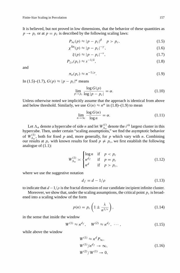
It is believed, but not proved in low dimensions, that the behavior of these quantities asp → pc or atp = pc is described by the following scaling laws:
P∞(p) ≈ |p − pc|β p > pc, (1.5)
χfin(p) ≈ |p − pc|−γ , (1.6)
ξ(p) ≈ |p − pc|−ν, (1.7)
P≥s(pc) ≈ s−1/δ, (1.8)
and
πn(pc) ≈ n−1/ρ. (1.9)
In (1.5)–(1.7),G(p) ≈ |p − pc|α means
limp→pc
logG(p)
log |p − pc| = α. (1.10)
Unless otherwise noted we implicitly assume that the approach is identical from aboveand below threshold. Similarly, we useG(n) ≈ nα in (1.8)–(1.9) to mean
limn→∞
logG(n)
logn= α. (1.11)
Letn denote a hypercube of siden and letW(i)n
denote theith largest cluster in thishypercube. Then, under certain “scaling assumptions,” we find the asymptotic behaviorof W(1)
n, both for fixedp and, more generally, forp which vary withn. Combining
our results atpc with known results for fixedp �= pc, we first establish the followinganalogue of (1.1):
W(1)n
�
logn if p < pc
ndf if p = pc
nd if p > pc,
(1.12)
where we use the suggestive notation
df = d − 1/ρ (1.13)
to indicate thatd−1/ρ is the fractal dimension of our candidate incipient infinite cluster.Moreover, we show that, under the scaling assumptions, the critical pointpc is broad-
ened into a scaling window of the form
p(n) = pc
(1± λ
n1/ν
), (1.14)
in the sense that inside the window
W(1) ≈ ndf , W(2) ≈ ndf , · · · , (1.15)
while above the window
W(1) ≈ ndP∞,
W(1)/ndf → ∞,
W(2)/W(1) → 0,
(1.16)
158 C. Borgs, J. T. Chayes, H. Kesten, J. Spencer
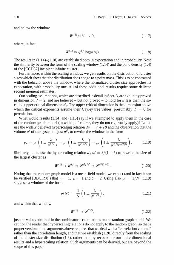
and below the window
W(1)/ndf → 0, (1.17)
where, in fact,
W(1) ≈ ξdf log(n/ξ). (1.18)
The results in (1.14)–(1.18) are established both in expectation and in probability. Notethe similarity between the form of the scaling window (1.14) and the bond density (1.4)of the [CCD87] incipient infinite cluster.
Furthermore, within the scaling window, we get results on the distribution of clustersizes which show that the distribution does not go to a point mass. This is to be contrastedwith the behavior above the window, where the normalized cluster size approaches itsexpectation, with probability one. All of these additional results require some delicatesecond moment estimates.
Our scaling assumptions, which are described in detail in Sect. 3, are explicitly provedin dimensiond = 2, and are believed – but not proved – to hold ford less than the so-called upper critical dimensiondc. The upper critical dimension is the dimension abovewhich the critical exponents assume their Cayley tree values; presumablydc = 6 forpercolation.
What would results (1.14) and (1.15) say if we attempted to apply them in the caseof the random graph model (to which, of course, they do not rigorously apply)? Let ususe the widely believed hyperscaling relationdν = γ + 2β and the observation that thevolumeN of our system is justnd , to rewrite the window in the form
pn = pc
(1± λ
n1/ν
)= pc
(1± λ
N1/dν
)= pc
(1± λ
N1/(γ+2β)
). (1.19)
Similarly, let us use the hyperscaling relationdf /d = δ/(1 + δ) to rewrite the size ofthe largest cluster as
W(1) ≈ ndf ≈ Ndf /d ≈ Nδ/(1+δ). (1.20)
Noting that the random graph model is a mean-field model, we expect (and in fact it canbe verified [BBCK98]) thatγ = 1, β = 1 andδ = 2. Using alsopc = 1/N , (1.19)suggests a window of the form
p(N) = 1
N
(1± λ
N1/3
), (1.21)
and within that window
W(1) ≈ N2/3, (1.22)
just the values obtained in the combinatoric calculations on the random graph model. Wecaution the reader that hyperscaling relations do not apply to the random graph, so that aproper version of the arguments above requires that we deal with a “correlation volume”rather than the correlation length, and that we establish (1.20) directly from the scalingof the cluster size distribution (1.8), rather than by recourse to our finite-dimensionalresults and a hyperscaling relation. Such arguments can be derived, but are beyond thescope of this paper.

Finite-Size Scaling in Percolation 159
Our results also have implications for finite-size scaling. Indeed, the form of thewindow tells us precisely how to locate the critical point, i.e., it tells us the correctregion aboutpc in which to do critical calculations.
Finally, the results tell us that we may use the largest cluster in the box as a candidatefor the incipient infinite cluster. Within the window, it is not unique, in the sense thatthere are many clusters of this scale. However, above the window (even including aregion wherep is not uniformly greater thanpc asn → ∞), there is a unique clusterof largest scale. This is the analogue of what is called thedominant component in therandom graph problem.
It is interesting to contrast our results with recent results in high dimensions. Asalready observed on a heuristic level in [Con85], the validity of hyperscaling is relatedto the fact that the critical crossing clusters in a box of side lengthn have size of ordernd−1/ρ , and that their number is bounded uniformly inn; see [BCKS98] for rigorousresults concerning this relationship. Conversely, breakdown of hyperscaling above sixdimensions requires, at least on a heuristic level, that at criticality, the number of crossingclusters in a box of side lengthn grows likend−6, and that all of them have sizes ofordern4; see again [Con85]. In a similar way, one would expect that thelargest clusterin a box of side lengthn is of sizen4, and that there are roughlynd−6 clusters of similarsize. Indeed, it can be proven [Aiz97] that these results follow from a postulate on thedecay of the connectivity function at criticality which is widely believed to hold abovesix dimensions. Very recently, T. Hara [Har01] used the so-called Lace expansion, in theform developed in [HHS01], to rigorously establish this postulate in sufficiently highdimensionsd � 6.
Methods and organization. As mentioned above, our results are proved under certainscaling assumptions which we explicitly verify in dimensiond = 2. Obviously, theresults could have been proven directly – with no assumptions – ind = 2, but theresulting proof would have been quite complicated and would not have yielded muchinsight. Instead, we formulate postulates which we believe characterize critical behaviorin all dimensions below the critical dimensiondc, and then prove our results under thesepostulates. We believe that the postulates are of independent interest since they provideinsight into the nature of critical behavior. Indeed, in previous announcements of thiswork [CPS96] and [Cha98], we used more postulates than we need now. In [BCKS98],we proved that one of these original postulates was implied by several others, in particularthat a reasonable assumption on the behavior of crossing probabilities implies certainhyperscaling relations among critical exponents.The proofs in this paper will rely heavilyon the results and methods of [BCKS98]. Indeed, [BCKS98] should really be viewedas “Part I” of this paper, since many of our results on the cluster size distribution werederived there. The verification of the postulates ind = 2 relies on the constructivetwo-dimensional methods of [Kes86] and [Kes87].
The organization of this paper is as follows. In Sect. 2, we give definitions, nota-tions and previous percolation results we will need in our proofs. Our main results areformulated in Sect. 3. There we first state our postulates, and then state the finite-sizescaling results under these postulates. In Sect. 4, we state many additional results whichmay be of independent interest, including the results of [BCKS98]. Finally, using theseadditional results, in Sect. 5 we prove our main finite-size scaling theorems under thescaling postulates. We believe, but cannot prove, that the scaling postulates should holdup to the upper critical dimension, which is believed to bedc = 6 for percolation. Finally,in Sect. 6, we prove that the scaling postulates are satisfied in two dimensions. Thus,we have a complete proof of finite-size scaling for percolation in dimensiond = 2. In
160 C. Borgs, J. T. Chayes, H. Kesten, J. Spencer
Sect. 7, we give a proof of slightly stronger finite-size scaling results under an alternativeset of postulates, and also show that the alternative postulates hold ind = 2.
2. Definitions, Notation and Preliminaries
Consider the hypercubic site latticeZd , and the corresponding bond latticeBd consisting
of bonds between all nearest-neighbor pairs inZd . Bond percolation onBd is defined
by choosing each bond ofBd to beoccupied with probabilityp andvacant with prob-ability 1− p, independently of all other bonds. The corresponding product measure onconfigurations of occupied and vacant bonds is denoted byPrp.Ep denotes expectationwith respect to the measurePrp, and Covp(· ; ·) denotes the covariance of two indicatorfunctions with respect toPrp: Covp(A;B) = Prp(A∩B)− Prp(A)Prp(B). A genericconfiguration is denoted byω. If S1, S2, S3 ⊂ Z
d , we say thatS1 is connected toS2 in S3,denoted by{S1 ↔ S2 in S3}, if there exists an occupied path with vertices inS3 fromsome site ofS1 to some site ofS2. Maximal connected subsets are called(occupied)clusters. The occupied cluster (in the configurationω) containing the sitex is denotedby C(x) = C(x;ω). The size of the clusterC, denoted by|C|, is the number of sites inC. C∞ denotes the (unique) infinite cluster, i.e., the occupied cluster with|C| = ∞.
We also consider clusters in a finite box ⊂ Zd . The connected component ofx
in C(x) ∩ is denoted byC(x) = C(x;ω); this is therefore the collection of allpoints which are connected tox by an occupied path in. C(1) , C(2) , · · · C(k) denote theoccupied clusters in, ordered from largest to smallest size, with lexicographic orderbetween clusters of the same size.W
(i) = |C(i) | denotes the size of theith largest cluster
in . Finally
N(s1, s2) = |{i | s1 ≤ W(i) ≤ s2}| (2.1)
denotes the number of clusters in with size betweens1 ands2, and
N(s1, s2) = |{i | s1 ≤ W(i) ≤ s2, C
(i) �↔ ∂}| (2.2)
is the corresponding number of clusters which do not touch the boundary∂ of .Here∂ is the set of pointsx ∈ that have distance less than 1 from the complementc = Z
d \ of .Returning now to the model on the full lattice, the cluster size distribution is charac-
terized by
Ps = Ps(p) = Prp(|C(0)| = s), (2.3)
or alternatively
P≥s = P≥s(p) = Prp(|C(0)| ≥ s). (2.4)
The order parameter of the model is thepercolation probability or infinite-cluster density
P∞(p) = Prp(|C(0)| = ∞). (2.5)
Thecritical probability is
pc = inf{p : P∞(p) > 0}. (2.6)
Finite-Size Scaling in Percolation 161
We consider several connectivity functions: the(point-to-point) connectivity function
τ(v,w;p) = Prp(v ↔ w), (2.7)
thefinite-cluster (point-to-point) connectivity function
τ fin(v,w;p) = Prp(v ↔ w, |C(v)| < ∞), (2.8)
thepoint-to-hyperplane connectivity function
πn(p) = Prp{∃ v = (n, ·) such that0 ↔ v} (2.9)
(v = (n, ·)means that the first coordinate ofv equalsn), and thepoint-to-box connectivityfunction
πn(p) = Prp{0 ↔ ∂Bn(0)}, (2.10)
where
Bn(v) = {w ∈ Zd : |v − w|∞ ≤ n} = [−n, n]d ∩ Z
d , (2.11)
with | · |∞ denoting the0∞-norm. Notice thatπn(p) andπn(p) are equivalent, in thesense that
πn(p) ≤ πn(p) ≤ 2dπn(p). (2.12)
A quantity which forp > pc behaves much likeτ fin(x, y;p) is the covariance:
τ cov(v,w;p) = Covp(v ↔ ∞;w ↔ ∞) (2.13)
(see [CCGKS89], Sect. 6). We also consider several susceptibilities:
χ(p) = Ep(|C(0)|) =∑v
τ (0, v;p), (2.14)
χfin(p) = Ep(|C(0)|, |C(0)| < ∞) =∑v
τ fin(0, v;p) =∑s<∞
sPs(p) (2.15)
and
χcov(p) =∑v
τ cov(0, v;p). (2.16)
Finally, we introduce the quantity
s(n) = (2n)d πn(pc). (2.17)
As we will see,s(n) is the order of magnitude of the size of the largest critical clusterson scalen.
Length scales in the model are naturally expressed in terms of the correlation lengthξ(p), defined by the limit
1/ξ(p) = − lim|v|∞→∞1
|v|∞ logτ fin(0, v;p), (2.18)
taken withv along a coordinate axis. We will use the fact thatξ(p) < ∞ for all p �= pcandξ(p) → ∞ asp ↑ pc (see Grimmett [Gri99], Theorem 6.49 and Eq. (6.57) for
162 C. Borgs, J. T. Chayes, H. Kesten, J. Spencer
p < pc; for p > pc this follows from Grimmett and Marstrand [GM90]). While it isalso believed thatξ(p) → ∞ asp ↓ pc, this is rigorously known only ford = 2.
Alternatively, lengths may be expressed in terms of the finite-size scaling correlationlengthL0(p, ε), introduced in [CCF85] and studied in [CCF85,CCFS86] and [Kes87].Forp < pc, L0(p, ε) is defined in terms of the crossing probabilities of rectangles, theso-calledsponge crossing probabilities:
RL,M(p) = Prp{ ∃ occupied bond crossing of[0, L] × [0,M] · · · × [0,M]in the 1-direction}. (2.19)
Observing that, forp < pc, the sponge crossing probabilityRL,3L(p) → 0 asL → ∞,we define
L0(p) = L0(p, ε) = min{L ≥ 1 | RL,3L(p) ≤ ε} if p < pc. (2.20)
Using the methods and results of [ACCFR83,CC86,CCF85] and [Kes87], it is straight-forward to show that there existsa(d) > 0 such that forε < a(d), the scaling behaviorof L0(p, ε) is independent ofε for p < pc, in the sense thatL0(p, ε1)/L0(p, ε2) isbounded away from 0 and infinity for two fixed valuesε1, ε2 < a(d). This scaling be-havior is also essentially the same as that of the standard correlation lengthξ(p). Morespecifically, for 0< ε < a(d), there exist constantsc1 = c1(d), c2 = c2(d, ε) < ∞such that1
1
L0(p, ε)≤ 1
ξ(p)≤ c1 logL0(p, ε)+ c2
L0(p, ε)− 1, p < pc. (2.21)
Hereafter we will assume thatε < a(d); we usually suppress theε-dependence in ournotation.
Forp > pc, it is natural to defineL0(p, ε) in terms of a suitable finite-cluster analogueof the sponge-crossing probabilityRL,M(p), see [CC87], Eq. (53). For technical reasons,it is convenient, however, to consider instead crossings in an annulus
HL,M = Zd ∩ [−L,L+M]d \ (0,M)d, (2.22)
with inner and outer boundaries∂IHL,M and∂EHL,M . We say that an occupied clusterCH in H = HL,M isH -finite if H \CH contains a path – occupied or not – that connects∂IH to ∂EH . Let
SfinL,M(p) = Prp{ ∃ an occupiedH -finite clusterCH in H = HL,M
that connects∂IH to ∂EH }, (2.23)
with the conventionSfin0,M(p) = 1. We define
L0(p) = L0(p, ε) = 1+ max{L ≥ 0 : SfinL,L(p) ≥ ε} if p > pc, (2.24)
and more generally, forx ≥ 1,
L0(p, ε; x) = 1+ max{L ≥ 0 : SfinL,�xL (p) ≥ ε} if p > pc. (2.25)
Note thatL0(p, ε; x) may be finite or infinite, depending on whether or not there existsanL0 < ∞ such thatSfin
L,�xL (p) < ε for all L ≥ L0. We expect that this definition
1 K. Alexander [Ale96] has shown that one can takec1(d = 2) = 0 in (2.21)
Finite-Size Scaling in Percolation 163
coincides, say in the sense of Eq. (2.21) (with anx−dependent constantc2, andc1(d) =0), with the standard correlation lengthξ(p) above threshold. However, we are not ableto prove this ind ≥ 3, since the rescaling techniques of [ACCFR83] do not work forfinite-cluster crossings. Ind = 2, we can use a Harris ring construction [Har60] inconjunction with the Russo–Seymour–Welsh Lemma ([Rus78,SW78]) to show that thisdefinition is equivalent toξ(p); see Sect. 6.
An important quantity in the high-density phase is the surface tensionσ(p); see[ACCFR83] for the precise definition. By analogy with the definition of a finite-sizescaling correlation length below threshold, we define a finite-size scaling inverse surfacetension as
A0(p) = A0(p, ε) = min{Ld−1 ≥ 1 | RL,3L(p) ≥ 1− ε} if p > pc. (2.26)
It is easy to see thatA0(p) is well-defined and finite for allp > pc. Indeed,p > pcimpliesP∞(p) > 0, which in turn implies that the probability of the event|C(x)| < ∞for all x ∈ Z
d ∩ [0, L]d goes to zero asL → ∞. Since this probability is bounded frombelow by(1−RL,3L(p))
2d (cf. the proof of Lemma 4.4), this implies thatRL,3L(p) →1 asL → ∞, and henceA0(p) is well-defined and finite. We expect thatA0(p) isequivalent to the inverse surface tension2 1/σ(p), which in turn should be equivalent toξd−1(p) below the critical dimensiondc (presumablydc = 6). Again, we are only ableto prove this equivalence ind = 2.
While the behavior ofL0(p) belowpc is well understood in general dimension, muchless is known aboutL0(p) or A0(p) abovepc. In particular, belowpc, it is easy to seethatL0(p) is monotone increasing, left continuous and piecewise constant. Moreover,
L0(p) ↑ ∞ as p ↑ pc, (2.27)
becauseRL,3L(pc) is bounded away from 0 (e.g., by Theorem 5.1 in [Kes82]). Further-more, the jumps inL0(p) are uniformly bounded on a logarithmic scale. In particular,by the methods of [ACCFR83,CC86,CCF85] and [Kes87], we have
R2L,6L ≤ 1
a(d)R2L,3L, (2.28)
which in turn implies
limδ→0
L0(p + δ)
L0(p)≤ 2, (2.29)
providedp < pc and ε < a(d). By contrast, none of these properties are knownfor L0(p) abovepc. Next considerA0(p), which, almost by definition, is monotonedecreasing and right continuous. However, in general dimension, we do not have a proofthatA0(p) diverges asp ↓ pc, nor do we have a bound of the form (2.29). We willtherefore require several postulates on the behavior ofL0(p) andA0(p) abovepc.
2 Using Proposition 3 of [CC87], one can actually prove thatA0(p) ≤ constσ(p)−1 for all d ≥ 2. Wedo not expect that the opposite inequality holds ford > the critical dimension,dc, since such an inequality –together with the usual assumption thatσ(p) → 0 asp ↓ pc – would imply thatA0(p) → ∞ asp ↓ pc ford > dc, which is believed to be false, see Sect. 3.3.
164 C. Borgs, J. T. Chayes, H. Kesten, J. Spencer
3. Statement of Postulates and Theorems
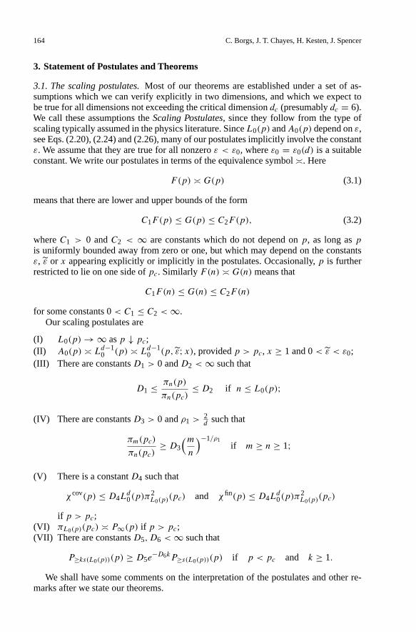
3.1. The scaling postulates. Most of our theorems are established under a set of as-sumptions which we can verify explicitly in two dimensions, and which we expect tobe true for all dimensions not exceeding the critical dimensiondc (presumablydc = 6).We call these assumptions theScaling Postulates, since they follow from the type ofscaling typically assumed in the physics literature. SinceL0(p) andA0(p) depend onε,see Eqs. (2.20), (2.24) and (2.26), many of our postulates implicitly involve the constantε. We assume that they are true for all nonzeroε < ε0, whereε0 = ε0(d) is a suitableconstant. We write our postulates in terms of the equivalence symbol�. Here
F(p) � G(p) (3.1)
means that there are lower and upper bounds of the form
C1F(p) ≤ G(p) ≤ C2F(p), (3.2)
whereC1 > 0 andC2 < ∞ are constants which do not depend onp, as long aspis uniformly bounded away from zero or one, but which may depend on the constantsε, ε or x appearing explicitly or implicitly in the postulates. Occasionally,p is furtherrestricted to lie on one side ofpc. SimilarlyF(n) � G(n) means that
C1F(n) ≤ G(n) ≤ C2F(n)
for some constants 0< C1 ≤ C2 < ∞.Our scaling postulates are
(I) L0(p) → ∞ asp ↓ pc;(II) A0(p) � Ld−1
0 (p) � Ld−10 (p, ε; x), providedp > pc, x ≥ 1 and 0< ε < ε0;
(III) There are constantsD1 > 0 andD2 < ∞ such that
D1 ≤ πn(p)
πn(pc)≤ D2 if n ≤ L0(p);
(IV) There are constantsD3 > 0 andρ1 >2d
such that
πm(pc)
πn(pc)≥ D3
(mn
)−1/ρ1if m ≥ n ≥ 1;
(V) There is a constantD4 such that
χcov(p) ≤ D4Ld0(p)π
2L0(p)
(pc) and χfin(p) ≤ D4Ld0(p)π
2L0(p)
(pc)
if p > pc;(VI) πL0(p)(pc) � P∞(p) if p > pc;(VII) There are constantsD5,D6 < ∞ such that
P≥ks(L0(p))(p) ≥ D5e−D6kP≥s(L0(p))(p) if p < pc and k ≥ 1.
We shall have some comments on the interpretation of the postulates and other re-marks after we state our theorems.
Finite-Size Scaling in Percolation 165
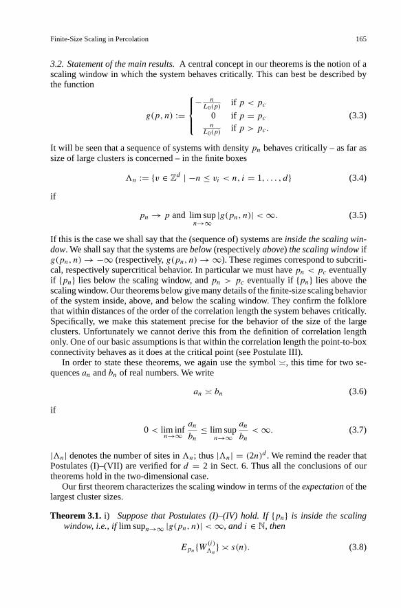
3.2. Statement of the main results. A central concept in our theorems is the notion of ascaling window in which the system behaves critically. This can best be described bythe function
g(p, n) :=
− n
L0(p)if p < pc
0 if p = pcn
L0(p)if p > pc.
(3.3)
It will be seen that a sequence of systems with densitypn behaves critically – as far assize of large clusters is concerned – in the finite boxes
n := {v ∈ Zd | −n ≤ vi < n, i = 1, . . . , d} (3.4)
if
pn → p and lim supn→∞
|g(pn, n)| < ∞. (3.5)
If this is the case we shall say that the (sequence of) systems areinside the scaling win-dow. We shall say that the systems arebelow (respectivelyabove) the scaling window ifg(pn, n) → −∞ (respectively,g(pn, n) → ∞). These regimes correspond to subcriti-cal, respectively supercritical behavior. In particular we must havepn < pc eventuallyif {pn} lies below the scaling window, andpn > pc eventually if{pn} lies above thescaling window. Our theorems below give many details of the finite-size scaling behaviorof the system inside, above, and below the scaling window. They confirm the folklorethat within distances of the order of the correlation length the system behaves critically.Specifically, we make this statement precise for the behavior of the size of the largeclusters. Unfortunately we cannot derive this from the definition of correlation lengthonly. One of our basic assumptions is that within the correlation length the point-to-boxconnectivity behaves as it does at the critical point (see Postulate III).
In order to state these theorems, we again use the symbol�, this time for two se-quencesan andbn of real numbers. We write
an � bn (3.6)
if
0 < lim infn→∞
an
bn≤ lim sup
n→∞an
bn< ∞. (3.7)
|n| denotes the number of sites inn; thus|n| = (2n)d . We remind the reader thatPostulates (I)–(VII) are verified ford = 2 in Sect. 6. Thus all the conclusions of ourtheorems hold in the two-dimensional case.
Our first theorem characterizes the scaling window in terms of theexpectation of thelargest cluster sizes.
Theorem 3.1. i) Suppose that Postulates (I)–(IV) hold. If {pn} is inside the scalingwindow, i.e., if lim supn→∞ |g(pn, n)| < ∞, and i ∈ N, then
Epn{W(i)n
} � s(n). (3.8)
166 C. Borgs, J. T. Chayes, H. Kesten, J. Spencer
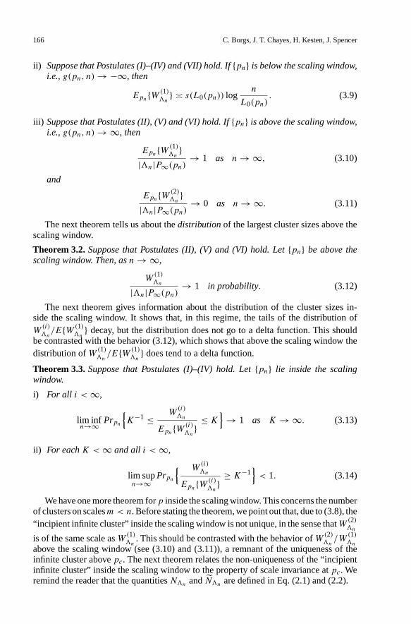
ii) Suppose that Postulates (I)–(IV) and (VII) hold. If {pn} is below the scaling window,i.e., g(pn, n) → −∞, then
Epn{W(1)n
} � s(L0(pn)) logn
L0(pn). (3.9)
iii) Suppose that Postulates (II), (V) and (VI) hold. If {pn} is above the scaling window,i.e., g(pn, n) → ∞, then
Epn{W(1)n
}|n|P∞(pn)
→ 1 as n → ∞, (3.10)
and
Epn{W(2)n
}|n|P∞(pn)
→ 0 as n → ∞. (3.11)
The next theorem tells us about thedistribution of the largest cluster sizes above thescaling window.
Theorem 3.2. Suppose that Postulates (II), (V) and (VI) hold. Let {pn} be above thescaling window. Then, as n → ∞,
W(1)n
|n|P∞(pn)→ 1 in probability. (3.12)
The next theorem gives information about the distribution of the cluster sizes in-side the scaling window. It shows that, in this regime, the tails of the distribution ofW
(i)n/E{W(1)
n} decay, but the distribution does not go to a delta function. This should
be contrasted with the behavior (3.12), which shows that above the scaling window thedistribution ofW(1)
n/E{W(1)
n} does tend to a delta function.
Theorem 3.3. Suppose that Postulates (I)–(IV) hold. Let {pn} lie inside the scalingwindow.
i) For all i < ∞,
lim infn→∞ Prpn
{K−1 ≤ W
(i)n
Epn{W(i)n
}≤ K
}→ 1 as K → ∞. (3.13)
ii) For each K < ∞ and all i < ∞,
lim supn→∞
Prpn{ W
(i)n
Epn{W(i)n
}≥ K−1
}< 1. (3.14)
We have one more theorem forp inside the scaling window. This concerns the numberof clusters on scalesm < n. Before stating the theorem, we point out that, due to (3.8), the“incipient infinite cluster” inside the scaling window is not unique, in the sense thatW
(2)n
is of the same scale asW(1)n
. This should be contrasted with the behavior ofW(2)n
/W(1)n
above the scaling window (see (3.10) and (3.11)), a remnant of the uniqueness of theinfinite cluster abovepc. The next theorem relates the non-uniqueness of the “incipientinfinite cluster” inside the scaling window to the property of scale invariance atpc. Weremind the reader that the quantitiesNn andNn are defined in Eq. (2.1) and (2.2).
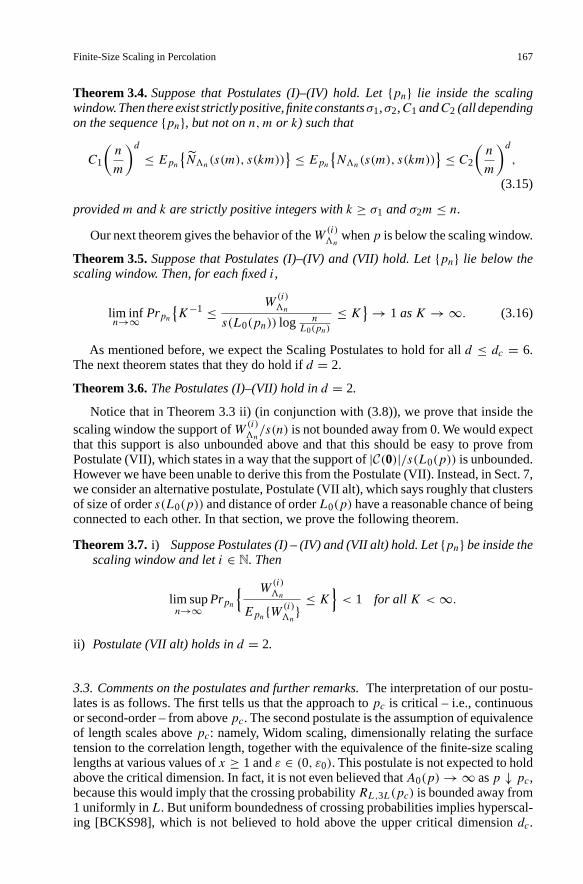
Finite-Size Scaling in Percolation 167
Theorem 3.4. Suppose that Postulates (I)–(IV) hold. Let {pn} lie inside the scalingwindow.Then there exist strictly positive, finite constantsσ1,σ2,C1 andC2 (all dependingon the sequence {pn}, but not on n,m or k) such that
C1
(n
m
)d≤ Epn
{Nn(s(m), s(km))
} ≤ Epn
{Nn(s(m), s(km))
} ≤ C2
(n
m
)d,
(3.15)
provided m and k are strictly positive integers with k ≥ σ1 and σ2m ≤ n.
Our next theorem gives the behavior of theW(i)n
whenp is below the scaling window.
Theorem 3.5. Suppose that Postulates (I)–(IV) and (VII) hold. Let {pn} lie below thescaling window. Then, for each fixed i,
lim infn→∞ Prpn
{K−1 ≤ W
(i)n
s(L0(pn)) log nL0(pn)
≤ K}→ 1 as K → ∞. (3.16)
As mentioned before, we expect the Scaling Postulates to hold for alld ≤ dc = 6.The next theorem states that they do hold ifd = 2.
Theorem 3.6. The Postulates (I)–(VII) hold in d = 2.
Notice that in Theorem 3.3 ii) (in conjunction with (3.8)), we prove that inside thescaling window the support ofW(i)
n/s(n) is not bounded away from 0. We would expect
that this support is also unbounded above and that this should be easy to prove fromPostulate (VII), which states in a way that the support of|C(0)|/s(L0(p)) is unbounded.However we have been unable to derive this from the Postulate (VII). Instead, in Sect. 7,we consider an alternative postulate, Postulate (VII alt), which says roughly that clustersof size of orders(L0(p)) and distance of orderL0(p) have a reasonable chance of beingconnected to each other. In that section, we prove the following theorem.
Theorem 3.7. i) Suppose Postulates (I) – (IV) and (VII alt) hold. Let {pn} be inside thescaling window and let i ∈ N. Then
lim supn→∞
Prpn{ W
(i)n
Epn{W(i)n
}≤ K
}< 1 for all K < ∞.
ii) Postulate (VII alt) holds in d = 2.
3.3. Comments on the postulates and further remarks. The interpretation of our postu-lates is as follows. The first tells us that the approach topc is critical – i.e., continuousor second-order – from abovepc. The second postulate is the assumption of equivalenceof length scales abovepc: namely, Widom scaling, dimensionally relating the surfacetension to the correlation length, together with the equivalence of the finite-size scalinglengths at various values ofx ≥ 1 andε ∈ (0, ε0). This postulate is not expected to holdabove the critical dimension. In fact, it is not even believed thatA0(p) → ∞ asp ↓ pc,because this would imply that the crossing probabilityRL,3L(pc) is bounded away from1 uniformly inL. But uniform boundedness of crossing probabilities implies hyperscal-ing [BCKS98], which is not believed to hold above the upper critical dimensiondc.
168 C. Borgs, J. T. Chayes, H. Kesten, J. Spencer
Postulate (III) tells us that the system within the correlation length behaves as it does atthreshold, at least as characterized by the behavior of the point-to-box connectivity func-tion. Postulate (IV) implies that the connectivity function has a lower bound of powerlaw behavior at threshold. Especially Postulates (III) and (IV) turn out to imply morethan is immediately apparent. Proposition 4.6 states that the cluster size distribution forclusters with diameters up to the correlation length behaves like the corresponding dis-tribution at threshold. This proposition also gives us a hyperscaling relation between theexponentsδ andρ, assuming that these exponents exist. We also obtain a scaling relationfor χ(p) in Proposition 4.8. Assuming power laws forχ andL0, and the relation (4.24),the assumed bound onρ1 in Postulate (IV) is equivalent to the very weak boundγ > 0.But it is known ([AN84]) thatχ(p) ≥ C1(pc − p)−1, p < pc, i.e.,γ ≥ 1 if it exists. Inthe light of this, Postulate (IV) seems very reasonable. The fifth and sixth postulates givevarious exponent relations, again provided that these exponents exist. Finally, the lastpostulate states that (in the subcritical region)s(L0(p)) is the natural scale for the clustersize distribution and that on this scale the tail of the distribution does not decay fasterthan exponentially. Proposition 4.8 provides an inequality in the opposite direction, i.e.,this decay is at least exponentially fast. See also Remark vi) below.
Remarks. i) Assuming the existence of the exponentρ, see (1.9), Theorem 3.1 impliesthat inside the scaling window the largest, second largest, third largest,..., clusters scalelike ndf , with df = d − 1/ρ, while below the scaling window the size of the largestcluster (and hence of all clusters) goes to zero on the scalendf .
ii) By Postulate (VI), and Lemma 4.5 below,
|n|P∞(pn)
s(n)= P∞(pn)
πn(pc)� πL0(pn)(pc)
πn(pc)→ ∞ (3.17)
above the scaling window. Statement iii of Theorem 3.1 therefore implies that
Epn{W(1)n
}s(n)
→ ∞ as n → ∞ (3.18)
above the scaling window.
iii) Assume that the critical exponentν, see Eq. (1.7), exists, and that an equivalenceof the form (2.21) holds forp > pc as well. Choosep−
n = sup{p < pc : L0(p) ≤ n}.Then by (2.29),L0(p
−n ) � n. Moreover,
L0(p−n ) ≈ ξ(p−
n ) ≈ |p−n − pc|−ν (3.19)
so thatpc − p−n ≈ n−1/ν .
Finally,{pn} is below the scaling window if lim infn→∞ log(pc−pn)/ logn > −1/ν.Similar statements hold to the right ofpc withp+
n := inf {p > pc : L0(p) ≤ n}, providedwe make the further assumption that
lim supp↓pc
limδ↓0
L0(p − δ)
L0(p)< ∞.
Thus under these various assumptions the scaling window has widthn−1/ν .It should be pointed out, though, that at present we do not have enough rigorous
knowledge of the behavior ofL0(p) as a function ofp to define the scaling window interms of the behavior of(pn−pc)/g
±n for suitable sequences{g±
n }. For instance, it is not
Finite-Size Scaling in Percolation 169
known that there exists a sequence{g−n } of positive numbers such thatn/L0(pn) → ∞
is equivalent to(pc − pn)/g−n → ∞ for pn < pc.
iv) It follows from (3.11) and Markov’s inequality that
W(2)n
|n|P∞(pn)→ 0 in probability (3.20)
above the scaling window. Combined with (3.12) this implies that, asn → ∞,
W(2)n
W(1)n
→ 0 in probability, (3.21)
providedg(pn, n) → ∞.
v) In a similar way, it follows from (3.9) that, asn → ∞,
W(1)n
s(n)→ 0 in probability, (3.22)
providedg(pn, n) → −∞.
4. Auxiliary Results
In this section, which is split into two subsections, we state several useful auxiliaryresults, most of which have been already proved in [BCKS98], which we will need forour proofs in Sect. 5. The first subsection gives a fundamental moment estimate andan exponential tail estimate for cluster sizes. These estimates show a close relationshipbetween the diameter and the size or volume of a large cluster.A cluster inn of diametersmall with respect ton usually has a volume which is small with respect tos(n). Webelieve – but could not prove – that the converse also holds, namely that a cluster inn
of diameter of ordern has with high probability a volume bigger than a small multipleof s(n). The second subsection contains various important properties of the quantitiesπn, Ps, P≥s andχ which are akin to the postulates.
Throughout, the basic parameterp is bounded away from 0 and 1, that is we restrictp to ζ0 ≤ p ≤ 1− ζ0 for some small strictly positiveζ0. No further mention ofζ0 willbe made. Many constantsCi appear in this paper. These are alwaysfinite and strictlypositive, even when this is not indicated. In different formulae the same symbolCi
may denote different constants. All these constants depend onε, d, ζ0 and the constantswhich appear in the postulates. This dependence will not be indicated in the notation.I [A] denotes the indicator function of the eventA.
All results in this section are proven under Postulates (I)–(IV) or a subset of these. Infact, none of the statements of this section rely directly on Postulates (I) and (II). Instead,they use the following two assumptions, which are much weaker than Postulates (I) and(II). The first is the assumption that the sponge crossing probabilities atpc are boundedaway from one, that is,
1− Rn,3n(pc) > ε, n ≥ 1, (4.1)
170 C. Borgs, J. T. Chayes, H. Kesten, J. Spencer
for someε > 0, and the second is the assumption that (4.1) can be extended top > pc,providedn ≤ L0(p). Actually, we only need the slightly weaker assumption that thereare some constantsε > 0 andσ3 > 0 such that
1− Rn,3n(p) > ε for all p > pc and all n ≤ σ3L0(p). (4.2)
To see that (4.1) follows from Postulates (I) and (II), we note that these postulates implythatA0(p) → ∞ asp ↓ pc, which in turn implies the statement (4.1). The bound (4.2)follows directly from Postulate (II), since, by the definition ofA0(p),
1− Rr,3r (p) > ε for rd−1 < A0(p) and p > pc.
By the equivalence ofA0(p) andL0(p)d−1 (see Postulate (II)) this means that there
exists someσ3 > 0 such that (4.2) holds forp > pc and alln ≤ σ3L0(p). We cautionthe reader that abovepc, the definition of the correlation lengthL0(p) in [BCKS98] isslightly different from the definition here (compare (2.17) in [BCKS98] to our Eq. (2.24)).However, as noted in Remark (vi) in [BCKS98], all results there remain valid for anydefinition of L0(p) abovepc that obeys Postulates (3.15) and (3.16) in [BCKS98].While Postulate (3.16) of [BCKS98] is identical to our Postulate (III), Postulate (3.15)in [BCKS98] is slightly stronger than our assumption (4.2) – the former corresponds to(4.2) withσ3 = 1. Here, we need only one result which uses Postulate (3.15), namelyTheorem 3.6 of [BCKS98], which we cite to establish the last statement in our Proposition4.8 below. However, a careful reading of the proof of Theorem 3.6 in Eqs. (5.32)–(5.35)of [BCKS98] shows that actually only our weaker assumption (4.2) is needed.
4.1. General moment estimates. The first lemma is a direct consequence of Postulate(IV). It is identical to Lemma 4.4 in [BCKS98].
Lemma 4.1. If Postulate (IV) holds, then for β > 1/ρ1 − 1 (and a fortiori for β >
d/2− 1 = (d − 2)/2) there exists constants C1 = C(β, d) and C2 = C2(d) such that
L∑m=0
(m+ 1)βπm(pc) ≤ C1Lβ+1πL(pc) if L ≥ 1, (4.3)
and
L∑m=0
(m+ 1)d−1π2m(pc) ≤ C2L
dπ2L(pc) if L ≥ 1. (4.4)
The next lemma, which is identical to Lemma 6.1 in [BCKS98], gives a basic momentestimate. Ford = 2 such an estimate was already given in [Ngu88].
Lemma 4.2. Assume Postulate (IV) holds. Define
V (L) := number of sites in L connected to ∂2L. (4.5)
Then for some constants Ci , it holds that
EpVk(L) ≤ C1k!
(C2L
dπL(pc))k
, (4.6)
Finite-Size Scaling in Percolation 171
provided p ≤ pc, k ≥ 1 and L ≥ 1. Consequently
Ep exp(tV (L)) ≤ C1[1− tC2LdπL(pc)]−1 (4.7)
whenever p ≤ pc and 0 ≤ t < [C2LdπL(pc)]−1. When Postulates (III) and (IV) hold,
then (4.6)and (4.7)remain valid for p > pc and L ≤ L0(p).
The next proposition, which is one of the main technical results of [BCKS98] (Propo-sition 6.3 in [BCKS98]), follows from the above moment estimate Lemma 4.2. It iscrucial for our proofs in Sects. 5.1 and 5.3.
Proposition 4.3. i) Assume that Postulate (IV) holds. Then there exist constants Ci
such that
Prp{W
(1)n
≥ xs(L0(p))}≤ C1
(n
L0(p)
)de−C2x (4.8)
if x ≥ 0, n ≥ L0(p), and p < pc. In particular
Prp
{W
(1)n
≥ ys(L0(pn)) log
(n
L0(pn)
)}→ 0 (4.9)
if y > d/C2 and g(pn, p) → −∞.ii) Assume that Postulate (IV) holds, and if p > pc, that also Postulate (III) holds. Then
there exist constants Ci such that
Prp{W
(1)n
≥ xs(n)}≤ C1e
−C2x if x ≥ 0 and n ≤ L0(p). (4.10)
iii) Assume that Postulates (III) and (IV) hold. Then there exist constants Ci such that
Prp{W
(1)n
≥ xs(L0(p))}≤ C1
(n
L0(p)
)dexp
[−C2x + C3
(n
L0(p)
)d](4.11)
if x ≥ 0, n ≥ L0(p) and p > pc.
The next lemma summarizes several additional results which follow from Postulate(IV). To state it, we introduce the diameter of a clusterC as
diam(C) = maxv,w∈C
|v − w|∞. (4.12)
Lemma 4.4. Assume that Postulate (IV) holds. Then there exist constants Ci such that
Prp{diam(C(0)) ≥ xL0(p)} ≤ C1πL0(p)(p)e−C2x if x ≥ 2 andp < pc, (4.13)
and
Prp{∃ clusterC in n with diam(C) ≤ yn and|C| ≥ xs(n)} ≤ C1y−de−C2x/y
d/2
(4.14)
if x ≥ 0, 0 < y ≤ 1, p ≤ pc and 4/y ≤ n ≤ L0(p).
172 C. Borgs, J. T. Chayes, H. Kesten, J. Spencer
Proof. The bound (4.14) was proved in [BCKS98], see Remark (xiii) at the end ofSection 6 in [BCKS98].
To prove (4.13) we note that forx ≥ 2,
Prp{diam(C(0)) ≥ xL0(p)}≤ Prp{0 ↔ ∂BL0(p) and∂BL0(p) is connected to at least
�x/2 distinct boxesBL0(p)(jL0(p)), j ∈ 2Zd \ {0}}
= πL0(p)(p)P rp{∂BL0(p) is connected to at least
�x/2 distinct boxesBL0(p)(jL0(p)), j ∈ 2Zd \ {0}}
(see (2.11) for the definition ofBn(v)). As in the proof of Proposition 6.3 (ii) of[BCKS98], (more precisely, as in the proof of the bound (6.39) in [BCKS98]), the renor-malized Peierls argument of Theorem 5.1 in [Kes82] shows that for suitable constantsC1, C2 the probability
Prp{∂BL0(p) is connected to at least
�x/2 distinct boxesBL0(p)(jL0(p)), j ∈ 2Zd \ {0}}
is bounded above byC1e−C2x . "#
4.2. Some important scaling properties. In this subsection we state a number of prop-erties of the functionsπn, Ps andχ(p), most of which have already been proved in[BCKS98]. The first lemma provides an upper bound forπm(pc)/πn(pc) which com-plements the lower bound of Postulate (IV).
Lemma 4.5. i) There are constants C1 < ∞ and C2 > 0 such that
πn(p)
πL0(p)(p)≤ C1e
−C2n/L0(p) if p < pc and n ≥ L0(p). (4.15)
ii) Assume that (4.1)holds for some ε > 0. Then
Prpc {∂Bn(0) ↔ ∂B3n(0)} ≤ 1− ε2d if n ≥ 1. (4.16)
iii) Assume that (4.1)holds for some ε > 0. Then there exist constants C1, ρ2 < ∞ suchthat
πm(pc)
πn(pc)≤ C1
(mn
)−1/ρ2if m ≥ n ≥ 1. (4.17)
Proof. Statements i) and iii) are the content of Theorem 3.8 of [BCKS98]. To prove ii),we show that for anyp ∈ [0,1] and anyn ≥ 1, one has
Prp{∂Bn(0) �↔ ∂B3n(0)} ≥ [1− R2n,6n(p)]2d . (4.18)
Indeed, by the definition ofRn,m, the probability that there is no occupied crossing inthe 1-direction of the block
[n,3n] × [−3n,3n]d−1 (4.19)
Finite-Size Scaling in Percolation 173
is equal to 1− R2n,6n. The cubeB3n(0) is the union ofBn(0) and the block in (4.19)plus 2d − 1 more blocks congruent to the block in (4.19). LetFn be the event that noneof these 2d blocks congruent to (4.19) has an occupied crossing in the short direction.Obviously, the eventFn implies that∂Bn(0) is not connected to∂B3n(0), so that theprobability on the left hand side of (4.18) is bounded from below by the probability ofFn. SincePrp{Fn} is at least[1−R2n,6n(p)]2d by the Harris–FKG inequality, the bound(4.18) follows. "#
The next proposition summarizes the results of Theorem 3.7 and the first statementof Theorem 3.4 in [BCKS98]. Assuming existence of the critical exponentsρ andδ, thefirst statement implies the hyperscaling relationdρ = δ + 1. The second statement isthe analogue of Postulate (III) forP≥s(p).
Proposition 4.6. Assume that (4.1)holds for some ε > 0 and that Postulate (IV) holds.Then there exists constants C1 > 0 and C2 < ∞ such that
C1πn(pc) ≤ P≥s(n)(pc) ≤ C2πn(pc). (4.20)
If Postulate (III) holds as well, then there exist constants C3 > 0, C4 < ∞ and 0 <
σ0 = σ0(ε, d) ≤ 1 such that
C3P≥s(n)(pc) ≤ P≥s(n)(p) ≤ C4P≥s(n)(pc) if n ≤ σ0L0(p). (4.21)
Our last two propositions in this section summarizes the results of several theoremsin [BCKS98], namely Theorem 3.5, Theorem 3.6 and Theorem 3.9. Proposition 4.8 inparticular has two upper bounds complementing lower bounds in the postulates, anda hyperscaling relation. Assuming the existence of the corresponding exponents, thisrelation impliesγ = (d − 2/ρ)ν.
Lemma 4.7. Assume Postulate (IV) holds. Then there exist constants 0 < Ci < ∞ suchthat
P≥xs(L0(p))(p)
πL0(p)(pc)≤ C1e
−C2x if p < pc and x ≥ 1. (4.22)
Proposition 4.8. Assume that (4.1)is valid for some ε > 0, and that Postulates (III) and(IV) hold. Then there exist constants 0 < Ci < ∞ such that, withσ0 as in Proposition 4.6,it holds that
P≥xs(L0(p))(p)
P≥s(σ0L0(p))(p)≤ C1 exp[−C2x] if x ≥ 1 and p < pc, (4.23)
and
C3L0(p)d [πL0(p)(pc)]2 ≤ χ(p) ≤ C4L0(p)
d [πL0(p)(pc)]2, p < pc. (4.24)
If (4.1)and (4.2)are valid for some ε > 0 and some σ3 > 0, and if Postulate (IV) holds,then there exists a constant C5 > 0 such that
C5L0(p)d [πL0(p)(pc)]2 ≤ χfin(p), p > pc. (4.25)
174 C. Borgs, J. T. Chayes, H. Kesten, J. Spencer
5. Proof of the Theorems, Given the Postulates
In this section, we prove our principal results, Theorems 3.1–3.5. The section is dividedinto three subsections. These correspond to the proof of results within, above and belowthe scaling window: Theorem 3.1 i), Theorem 3.3 and Theorem 3.4 in Sect. 5.1, Theorem3.1 iii) and Theorem 3.2 in Sect. 5.2, and finally, Theorem 3.1 ii) and Theorem 3.5 inSect. 5.3.
5.1. Inside the scaling window. We start this subsection with several lemmas and propo-sitions concerning the numbersN(s1, s2) andN(s1, s2) of clusters with size betweens1 ands2, defined in (2.1) and (2.2). Although some of these results are very similar tothe theorems we are finally going to prove, we give them as separate propositions, sincethis allows us to better keep track of which postulates are needed in which step.
At many points in this and the following subsections, we use the fact that, for anarbitrary configurationω, and numberα, it holds that∑
i≥1
[W
(i)
]α =∑v∈
∑s≥1
sα−1I [|C(v)| = s]. (5.1)
This is obvious from the fact that in the right-hand side, the sum ofI [|C(w)| = s] overall pointsw in C(v) equalssI [|C(v)| = s]. Taking expectations of (5.1) gives∑
i≥1
Ep
{[W
(i)
]α} =∑v∈
∑s≥1
sα−1Prp {|C(v)| = s} . (5.2)
This argument forα = 1 will be used in the proof of Proposition 5.5, but even moreoften will we use the special caseα = 0, which says that the number of clusters of sizes can be rewritten as∣∣{i | W(i)
= s}∣∣ = ∑
v∈
1
sI [|C(v)| = s]. (5.3)
These formulae and some variants form a basic relationship which allows us to relateestimates on the distributions ofW(i)
and|C(0)|. We use the following consequence of(5.3):
Ep
{N(s1, s2)
} =s2∑
s=s1
∑v∈
1
sPrp
{|C(v)| = s}. (5.4)
In a similar way, we have
Ep
{N(s1, s2)
} =s2∑
s=s1
∑v∈
1
sPrp
{|C(v)| = s, v �↔ ∂}. (5.5)
We also need the corresponding representation for the expectation ofN2(s1, s2):
Ep
{N2(s1, s2)
} =∑
s1≤s≤s2s1≤s≤s2
∑v,w∈
1
ssPrp
{|C(v)| = s,
v �↔ ∂, |C(w)| = s, w �↔ ∂}.
(5.6)
The next two lemmas will be useful in proving lower bounds forW(i) .
Finite-Size Scaling in Percolation 175
Proposition 5.1. Assume that (4.1) holds for some ε > 0 and that Postulates (III) and(IV) hold. Then there exist constants 0 < Ci < ∞ and 1 ≤ σ1 < ∞ such that
C1
(n
m
)d≤ Ep
{Nn(s(m), s(km))
} ≤ Ep
{Nn(s(m), s(km))
} ≤ C2
(n
m
)d, (5.7)
provided σ1m ≤ min{L0(p), n} and k ≥ σ1.
Proof. For brevity we write instead ofn. We start with the upper bound. Using therepresentation (5.4) and bounding the factor 1/s in (5.4) by 1/s(m), we get
Ep
{N(s(m), s(km))
} ≤ 1
s(m)
∑v∈
∑s≥s(m)
Prp{|C(v)| = s
}= 1
s(m)
∑v∈
Prp{|C(v)| ≥ s(m)
}≤ (2n)d
s(m)P≥s(m)(p),
(5.8)
where in the last step we used the definition (2.4) ofP≥s(m)(p)and the fact that|C(v)| ≤|C(v)|.Without loss of generality we shall takeσ1 ≥ 1/σ0 ≥ 1, whereσ0 is the constant ofProposition 4.6. Thenσ1m ≤ L0(p) impliesm ≤ σ0L0(p), and we may use Proposition4.6 to bound the right-hand side of (5.8). We get for some finite constantC2,
(2n)d
s(m)P≥s(m)(p) ≤ C2
(2n)d
s(m)πm(pc) = C2
(n
m
)d. (5.9)
The estimates (5.8) and (5.9) imply the upper bound.To prove the lower bound, we use that Postulate (IV) implies that
s(0)
s(0′)≥ D3
( 00′)d/2
if 0 ≥ 0′ ≥ 1, (5.10)
so that in particulars(0) ≥ s(0′) whenever0/0′ ≥ D−2/d3 . We conclude that for any
choice ofk ≥ 1 we can find aσ1 ≥ k(1+1/σ0) such thats(km) ≥ s(km) for all k ≥ σ1.It then follows from (5.5) that fork ≥ σ1,
Ep
{N(s(m), s(km))
} ≥ Ep
{N(s(m), s(km)− 1)
}≥
s(km)−1∑s=s(m)
∑v∈n
2
1
sPrp
{|C(v)| = s, v �↔ ∂}
=s(km)−1∑s=s(m)
∑v∈n
2
1
sPrp
{|C(v)| = s, v �↔ ∂},
(5.11)
176 C. Borgs, J. T. Chayes, H. Kesten, J. Spencer
where in the second step we bounded the sum over = n from below by a sum overn
2. Bounding the factor 1/s in (5.11) from below by 1/s(km), we get
Ep
{N(s(m), s(km))
}≥ 1
s(km)
∑v∈n
2
Prp{s(m) ≤ |C(v)| < s(km), v �↔ ∂
}= 1
s(km)
∑v∈n
2
[Prp
{s(m) ≤ |C(v)| < s(km)
}− Prp
{s(m) ≤ |C(v)| < s(km), v ↔ ∂
}]
≥ 1
s(km)
∑v∈n
2
[Prp
{s(m) ≤ |C(v)| < s(km)
}− πn/2(p)]
≥ (n− 2)d
s(km)
[P≥s(m)(p)− P≥s(km)(p)− πn/2(p)
].
(5.12)
Sincen ≥ σ1m ≥ km by the assumptionσ1m ≤ min{L0(p), n}, we obtain
Ep
{N(s(m), s(km))
}≥ (n− 2)d
s(km)
[P≥s(m)(p)− P≥s(km)(p)− πkm/2(p)
]. (5.13)
Again by the assumptionσ1m ≤ min{L0(p), n}, we havem ≤ km ≤ (k/σ1)L0(p) ≤σ0L0(p). We therefore may use Proposition 4.6 in conjunction with Postulate (III) andthe boundπkm(pc) ≤ πkm/2(pc) to conclude that
Ep
{N(s(m), s(km))
} ≥ (n− 2)d
s(km)
[C3πm(pc)− C4πkm/2(pc)
], (5.14)
for suitable constantsC3, C4 ∈ (0,∞)which depend only on the constants in Proposition4.6, but not on the choice ofk. Finally we appeal to Lemma 4.5 iii) to fixk so largethatC4πkm/2(pc) ≤ 1
2C3πm(pc). Herek depends only onC4/C3 and the constants in
Lemma 4.5 iii); alsok determines the value to take forσ1. We then get
Ep
{N(s(m), s(km))
} ≥ (n− 2)d
s(km)
12C3πm(pc). (5.15)
Froms(km) ≤ kd s(m) we then conclude that forn ≥ 4,
Ep
{N(s(m), s(km))
} ≥ C1(2n)d
s(m)πm(pc) = C1
(n
m
)d, (5.16)
whereC1 = 2−2d−1k−dC3. This proves the lower bound whenn ≥ 4. If we chooseσ1large enough, then 1≤ n < 4 is ruled out byσ1 ≤ σ1m ≤ n. "#
Finite-Size Scaling in Percolation 177
Proposition 5.2. Assume that (4.1) holds for some ε > 0 and that Postulates (III) and(IV) hold. Then there is a constant C3 < ∞, such that
Var{Nn(s(m), s(km))
}Ep
{N(s(m), s(km))
}2 ≤ C3, (5.17)
provided σ1m ≤ min{L0(p), n}, k ≥ σ1. Here σ1 is the constant of Proposition 5.1.
Proof. Again we write forn. We first will prove that for arbitrarys1, s2 ∈ N, s1 ≤ s2,andp ∈ (0,1),
Ep
{[N(s1, s2)]2
}≤ Ep
{N(s1, s2)
} [1+ (2n)d
s1P≥s1(p)
]. (5.18)
We need some notation. We denote the set of bonds with both endpoints in byB(),and the set of bonds with both endpoints in\∂ by B(). LetB be a subset ofB().With a slight abuse of notation, we say thatv is a point inB if v is an endpoint of one ofthe bonds inB. We writeB is occupied (vacant) for the event thatall bonds inB ⊂ B()
are occupied (respectively, vacant). Givenv ∈ , we denote the set of all connectedsubsetsB ⊂ B() that contain the pointv by Bv(). Again with a slight abuse ofnotation, we denote the number of points in a clusterB ⊂ Bv() by |B|. Finally, wewrite ∂AB for the set of all bondsb ∈ B() \ B which share an endpoint with a bondb′ ∈ B.
Using Eq. (5.6), we rewrite the left-hand side of (5.18) as
Ep
{N(s1, s2)
2}=
∑v,w∈
∑B∈Bv()s1≤|B|≤s2
∑B∈Bw()
s1≤|B|≤s2
Prp{B ∪ B is occupied, ∂AB ∪ ∂AB is vacant
}|B| |B| . (5.19)
Next we observe that the event on the right-hand side cannot occur ifB ↔ B andB �= B
in , because in this case some occupied bond inB ∪ B∪ (a suitable path fromB toB) also lies in∂AB ∪ ∂AB. As a consequence, the right-hand side decomposes into twoterms: the term∑
v,w∈
∑B∈Bv()∩Bw()
s1≤|B|≤s2
Prp{B is occupied, ∂AB is vacant
}|B|2
=∑v∈
∑B∈Bv()s1≤|B|≤s2
Prp{B is occupied, ∂AB is vacant
}|B|
= Ep
{N(s1, s2)
}(5.20)
and the term∑v,w∈
∑B∈Bv()s1≤|B|≤s2
∑B∈Bw()
s1≤|B|≤s2,B �↔B
Prp{B ∪ B is occupied, ∂AB ∪ ∂AB is vacant}|B| |B| . (5.21)
178 C. Borgs, J. T. Chayes, H. Kesten, J. Spencer
By using the second decoupling inequality of [BC96], or, alternatively, the van denBerg-Kesten inequality [BK85] we see that the last sum equals
∑v,w∈
∑B∈Bv()\Bw()
s1≤|B|≤s2
∑B∈Bw()
s1≤|B|≤s2
Prp{B ∪ B is occupied, ∂AB ∪ ∂AB is vacant}|B| |B|
≤∑
v,w∈
1
s1
∑B∈Bv()\Bw()
s1≤|B|≤s2
Prp{B is occupied, ∂AB is vacant, |C(w)| ≥ s1}|B|
≤∑
v,w∈
1
s1
∑B∈Bv()\Bw()
s1≤|B|≤s2
Prp{B is occupied, ∂AB is vacant} Prp{|C(w)| ≥ s1}|B|
≤ Ep
{N(s1, s2)
} ∑w∈
Prp{|C(w)| ≥ s1}s1
.
(5.22)
Combining the two terms (5.20) and (5.22), and observing thatPrp {|C(w)| ≥ s1} ≤Prp{|C(w)| ≥ s1}, we obtain (5.18). The bound (5.17) now follows from (5.18), (5.9)and the lower bound in (5.7)."#
The next proposition is a consequence of Proposition 5.1, Proposition 5.2 and thefact that
N(s(m), s(km)) ≥ N1(s(m), s(km))+ N2(s(m), s(km)),
provided1 ⊂ and2 = \1.
Proposition 5.3. Assume that (4.1) holds for some ε > 0 and that Postulates (III) and(IV) hold. Then there are constants C4, C5 > 0 such that
Prp
{Nn(s(m), s(km)) ≥ C4
(n
m
)d}≥ 1− C5
(m
n
)d, (5.23)
provided σ1m ≤ min{L0(p), n} and k ≥ σ1. Here σ1 is the constant of Proposition 5.1.
Proof. Let k = �n/'σ1m( be the largest integer less than or equal ton/'σ1m(, andn = k'σ1m(. Note that thenσ1m ≤ n ≤ n. SinceN(s(m), s(km)) is increasing in,i.e.,
N(s(m), s(km)) ≥ N(s(m), s(km)) if ⊂ , (5.24)
we get that for = n, = n,
Prp
{N(s(m), s(km)) ≥ C4
(n
m
)d}≥ Prp
{N(s(m), s(km)) ≥ C4
(n
m
)d}.
(5.25)
Finite-Size Scaling in Percolation 179
Next we note that containskd disjoint subvolumes(i) of size(2'σ1m()d , and intro-duce the random variable
X =kd∑i=1
N(i) (s(m), s(km)). (5.26)
SinceX ≤ N(s(m), s(km)) ≤ N(s(m), s(km)), we have
Prp
{N(s(m), s(km)) ≥ C4
(n
m
)d}≥ Prp
{X ≥ C4
(n
m
)d}. (5.27)
Observing that the random variablesN(i) (s(m), s(km)) in (5.26) are i.i.d. and usingProposition 5.2, we have
VarX
(EpX)2= 1
kd
Var{N(1) (s(m), s(km))}Ep{N(1) (s(m), s(km))}2 ≤ C6
kd. (5.28)
Noting that
Prp{X ≤ 1
2EpX} ≤ Prp
{|X − EpX|2 ≥ 14(EpX)
2} ≤ 4 VarX
(EpX)2, (5.29)
we find that
Prp{X ≥ 1
2EpX} ≥ 1− 4C6
kd≥ 1− C5
(m
n
)d, (5.30)
whereC5 = (4σ1)d4C6 (note that 1/k = �n/'σ1m( −1 ≤ 4σ1m/n). Using finally the
lower bound
EpX = kdEp
{N(1) (s(m), s(km))
} ≥ C1(kσ1)d = C1
(n
m
)d,
which comes from (5.7), we obtain the desired bound (5.23), providedC4 > 0 is chosensmall enough. "#Proposition 5.4. Suppose that Postulates (III) and (IV) hold, and that (4.1) and (4.2)are valid for some ε > 0 and some σ3 > 0. Then there are strictly positive constants C1and σ4 such that
Prp{W
(1)n
≤ s(m)}≥ C
1+(n/m)d1 , (5.31)
provided m ≤ σ4L0(p).
Proof. It follows from (4.10) and (5.10) that there exists a constantσ4 > 0 such that
Prp{W
(1)3r
≤ s(m)}≥ 1
2if r ≤ σ4m andr ≤ 1
3L0(p). (5.32)
In addition, it follows (4.18) that
Prp {v �↔ ∂3r for all v ∈ r} ≥ [1− Rr,3r (p)]2d . (5.33)
180 C. Borgs, J. T. Chayes, H. Kesten, J. Spencer
Forp ≤ pc,
1− Rr,3r (p) ≥ 1− Rr,3r (pc) > ε
(see (4.1)). We still have 1− Rr,3r (p) > ε for p > pc andr ≤ σ3L0(p), by virtue of(4.2). Consequently, as in (4.16),
Prp {v �↔ ∂B3r for all v ∈ r} ≥ ε2d if r ≤ σ3L0(p). (5.34)
Using the Harris-FKG inequality we obtain from (5.32) and (5.34) that
Prp{|C(v)| ≤ s(m) for all v ∈ r
}≥ Prp
{W
(1)3r ≤ s(m) andv �↔ ∂B3r for all v ∈ r
}≥ 1
2ε2d if r ≤ (σ3 ∧ 1/3)L0(p) ∧ σ4m.
(5.35)
We are now ready to prove (5.31) for arbitraryn. We first estimate
Prp{W
(1) ≤ s(m)
}≥ Prp
{|C(v)| ≤ s(m) for all v ∈
}(5.36)
and note that the right-hand side of (5.36) is decreasing in. Let m ≤ σ4L0(p) andchoose 0< σ5 ≤ σ4 such thatσ4σ5 ≤ (σ3 ∧ 1/3). Then choose an integerr ≥ 1 in[σ5m/2, σ5m]; if this is not possible, becauseσ5m < 1, then taker = 1. For this choiceof r,
Prp {|C(v)| ≤ s(m) for all v ∈ r} ≥ C1 > 0
for some constantC1, by virtue of (5.35). Ifn < r, then this already implies (5.31).Otherwise, choose an integerk such thatn ≤ n := kr ≤ 2n. We then get
Prp{W
(1)n
≤ s(m)}≥ Prp
{ ⋂v∈n
{|C(v)| ≤ s(m)}}. (5.37)
Decomposingn into kd subvolumes(i) of diameter 2r, and using the Harris-FKGinequality for the intersection of the events∩v∈(i){|C(v)| ≤ s(m)}, we obtain
Prp{W
(1)n
≤ s(m)}≥[
Prp
{ ⋂v∈r
{|C(v)| ≤ s(m)}}]kd
≥ Ckd
1 . (5.38)
The proof is concluded by observing thatk ≤ 2n/r ≤ 4n/(σ5m). "#Proof of Theorem 3.1 i). For this proof we only use (4.1) and Postulates (III) and (IV).As before, abbreviaten to. Since lim supn→∞ |g(pn, n)| < ∞, we have
n ≤ λL0(pn) for all n ≥ n1, (5.39)
whereλ andn1 are finite constants depending on the sequence{pn}.The fact thatEp
{W
(1)
}/s(n) is bounded above is immediate from Proposition 4.3.
If n ≤ L0(pn) then (4.10) suffices. IfL0(pn) ≤ n ≤ λL0(pn), then we use (4.8) or(4.11) plus the fact thats(n) ≥ D3s(L0(pn)) (by (5.10)). Note that this proof onlyrequires Postulates (III) and (IV), and does not rely on the assumption (4.1).
Finite-Size Scaling in Percolation 181
In order to complete the proof, we need lower bounds onEp
{W
(i)
}. To this end, we
first note that Proposition 5.3 implies that for anyδ > 0 there are constants 1≤ σ (i) =σ (i)(λ, δ) < ∞ such that
Prp{W
(i)n
≥ s(m)}≥ 1− δ, (5.40)
providedσ (i)m ≤ n ≤ λL0(p). Indeed, chooseσ (i)(λ, δ) ≥ σ1 (with the constantσ1 as in Proposition 5.1) so large that i)σ (i)m ≤ λL0(p) implies σ1m ≤ L0(p), ii)C4(σ
(i))d ≥ i, and iii) C5(σ(i))−d ≤ δ, whereC4, C5 are as in Proposition 5.3. Then
for σ (i)m ≤ n ≤ λL0(p), we get
Prp{W
(i) ≥ s(m)
} = Prp{N(s(m),∞) ≥ i
} ≥ Prp{N(s(m), s(σ1m)) ≥ i
}≥ Prp
{N(s(m), s(σ1m)) ≥ C4
( nm
)d},
(5.41)
where we used thatσ (i)m ≤ n impliesC4(n/m)d ≥ i in the last step. Combined with
Proposition 5.3 and the fact that the assumptionσ (i)m ≤ n impliesC5(m/n)d ≤ δ by
our choice ofσ (i), the bound (5.41) implies (5.40).In order to prove a lower bound on lim inf
n→∞ Epn{W(i)n
}, we now assume thatn ≥ n(i)1 :=
max{n1, σ(i)}, wheren1 andλ are the constants from (5.39), andσ (i) = σ (i)(λ, 1
2).Choosingm = �n/σ (i) , we havem ≥ 1 andσ (i)m ≤ n ≤ λL0(pn). Thus, by (5.40)
Epn
{W
(i)n
} ≥ 12s(m). (5.42)
Sincem ≤ n/σ (i) ≤ m+ 1 ≤ 2m by the definition ofm, we have
s(n)/s(m) ≤ (n/m)d ≤ (2σ (i))d , (5.43)
and hences(m) ≥ s(n)(2σ (i))−d . Thus, withC(i)1 (λ) = 1
2(2σ(i))−d , we have
Epn
{W
(i)n
} ≥ C(i)1 (λ)s(n). (5.44)
This completes the proof of the lower bound."#
Proof of Theorem 3.3. For this proof use (4.1), (4.2) and Postulates (III) and (IV). Westart with a lower bound onPrpn
{W
(i)n
≥ K−1Epn(W(i)n)}. We again have (5.39) for
someλ andn1, and by Theorem 3.1 i) (whose proof only used (4.1) and Postulates (III)and (IV)) there exists some constantC
(i)2 , which depends on the sequence{pn}, such
that
Epn
{W
(i)n
} ≤ C(i)2 s(n).
Thus ifm is such that
s(m) ≥ K−1C(i)2 s(n), (5.45)
then
Prpn{W
(i)n
≥ K−1Epn
{W
(i)n
}} ≥ Prpn{W
(i)n
≥ s(m)}. (5.46)
182 C. Borgs, J. T. Chayes, H. Kesten, J. Spencer
We now choosem = �n/σ (i)(λ, δ) , where theσ (i) are the constants introduced above(5.40). Then (5.45) will be satisfied for large enoughK (by (5.43)). Sincen ≥ n1 andn ≥ σ (i)(λ, δ) impliesm ≥ 1 andmσ(i)(λ, δ) ≤ n ≤ λL0(pn), we now can use (5.40)to conclude that
lim infn→∞ Prpn
{W
(i)n
≥ K−1Epn
{W
(i)n
}} ≥ 1− δ, (5.47)
providedK is large enough. Together with Markov’s inequality,
Prpn{W
(i)n
≥ KEpn
{W
(i)n
}} ≤ K−1, (5.48)
(5.47) implies Theorem 3.3 i).In order to complete the proof of Theorem 3.3, we choosem(n) as the maximal
m ≤ (σ4/λ ∧ 1)n such thatK−1C(i)1 (λ)s(n) > s(m), whereσ4 is as in Proposition 5.4,
λ as in (5.39) andC(i)1 as in (5.44). Then, by (5.44) andW(i)
≤ W(1) , we have
lim supn→∞
Prpn{W
(i)n
≥ K−1Epn
{W
(i)n
}} ≤ lim supn→∞
Prpn{W
(i)n
≥ K−1C(i)1 (λ)s(n)
}≤ lim sup
n→∞Prpn
{W
(1)n
≥ K−1C(i)1 (λ)s(n)
}≤ lim sup
n→∞
[1− Prpn
{W
(1)n
≤ s(m(n))}].
(5.49)
Sincen/m(n) is bounded above by virtue of Postulate (IV) (see (5.10)), Proposition 5.4shows that the right-hand side of (5.49) is bounded away from 1. This proves Theorem3.3 ii). "#
Proof of Theorem 3.4. For this proof we only use (4.1), and Postulates (III) and (IV).Theorem 3.4 follows immediately from Proposition 5.1. Indeed, letλ andn1 be theconstants from (5.39), andC1, C2 andσ1 be those from Proposition 5.1. Chooseσ2 ≥max{σ1, λσ1, n1}. We note that thenm ≥ 1 andσ2m ≤ n imply n ≥ n1, and hencen ≤ λL0(pn) andσ1m ≤ L0(pn). The conditions of Theorem 3.4 therefore imply thoseof Proposition 5.1, proving that Theorem 3.4 under the assumption that (4.1), as well asPostulates (III) and (IV), hold. "#
5.2. Above the scaling window. In this subsection, we prove Theorem 3.1 iii) and The-orem 3.2. To this end, we consider separately those clustersC(i) which intersect theinfinite clusterC∞ and those which do not. We denote the clusters intersectingC∞ byC(1),∞, C(2),∞, · · · C(k),∞, ordering them again from largest to smallest size, with lexico-
graphic order between clusters of the same size. In the same way,C(1),fin, C(2),fin, · · · C(k),fin
denote the clusters in which do not intersect the infinite clusterC∞. Finally,W(i),fin =
|C(i),fin| andW(i),∞ = |C(i),∞| denote the sizes of theith largest clusters in the corre-
sponding classes.
Finite-Size Scaling in Percolation 183
Proposition 5.5. Suppose that Postulates (V) and (VI) hold. Then there exists a constantC1 < ∞ such that
Ep{W(1)n,fin}
|n|P∞(p)≤ C1
(L0(p)
n
)d/2if p > pc, (5.50)
so that in particular
Epn{W(1)n,fin}
|n|P∞(pn)→ 0 as n → ∞ (5.51)
whenever pn > pc is a sequence of densities such that n/L0(pn) → ∞ as n → ∞.
Proof. Let t (n) = (2nL0(p))d/2πL0(p)(pc). Analogously to (5.2) we have
Ep{W(1)n,fin} ≤ t (n)+ Ep{W(1)
n,fin;W(1)n,fin ≥ t (n)}
≤ t (n)+∑v∈n
Prp{|Cn(v)| = W(1)n,fin, |Cn(v)| ≥ t (n), v �↔ ∞}
≤ t (n)+ |n|Prp{|C(0)| ≥ t (n), 0 �↔ ∞}.(5.52)
Using Markov’s inequality and Postulate (V) we obtain
Ep{W(1)n,fin} ≤ t (n)+ (2n)d
t (n)χfin(p)
≤ t (n)+D4(2n)d
t (n)Ld
0(p)π2L0(p)
(pc)
= t (n)(1+D4
).
(5.53)
Observing thatt (n)/|n|P∞(p) � (L0(p)/n)d/2 by Postulate (VI), we obtain (5.50)
and hence (5.51)."#In order to estimate the size of the clustersC(1),∞, C(2),∞, · · · C(k),∞, we make extensive
use of the facts that∑i≥1
W(i),∞ = |n ∩ C∞| =
∑v∈n
I [v ↔ ∞] (5.54)
and
Epn{|n ∩ C∞|} =∑v∈n
Prpn{v ↔ ∞} = |n|P∞(pn). (5.55)
Lemma 5.6. Suppose that Postulates (V) and (VI) hold. Let pn > pc be a sequence ofdensities such that n/L0(pn) → ∞ as n → ∞. Then as n → ∞,
|n ∩ C∞||n|P∞(pn)
→ 1 in probability. (5.56)
184 C. Borgs, J. T. Chayes, H. Kesten, J. Spencer
Proof. We bound the variance of|n ∩ C∞| by
Varpn
{|n ∩ C∞|} =∑
v,w∈n
Covpn(v ↔ ∞;w ↔ ∞)
≤∑v∈nw∈Zd
Covpn(v ↔ ∞;w ↔ ∞) = |n|χcov(pn).(5.57)
Note that we used here the positivity of Covpn(v ↔;w ↔ ∞); this follows from theHarris–FKG inequality. Combined with (5.55) and Postulates (V) and (VI), we obtainthat for a suitable constantC1 < ∞,
Varpn{|n ∩ C∞|}E2pn
{|n ∩ C∞|} ≤ C1L0(pn)d
|n| = C1
(L0(pn)
2n
)d. (5.58)
By our assumption onpn, the right-hand side goes to zero asn → ∞. This implies(5.56). "#Proposition 5.7. Suppose that Postulates (II), (V) and (VI) hold. Let pn > pc be asequence of densities such that n/L0(pn) → ∞ as n → ∞. Then, as n → ∞,
W(1)n,∞
|n|P∞(pn)→ 1 in probability. (5.59)
Proof. We have to show that for allδ > 0
Prpn{W(1)n,∞ ≥ (1− δ)|n|P∞(pn)} → 1 asn → ∞ (5.60)
and
Prpn{W(1)n,∞ ≤ (1+ δ)|n|P∞(pn)} → 1 asn → ∞. (5.61)
SinceW(1)n,∞ ≤ |n ∩ C∞| by (5.54), the result (5.61) follows from (5.56). We are
therefore left with proving (5.60). Again by (5.56), this amounts to showing that withhigh probability, the main contribution to the left-hand side of (5.54) comes fromW
(1)n,∞.
We consider suitable volumesm ⊂ n with
limn→∞ |m|/|n| > 1− δ. (5.62)
Since
|C∞ ∩m||m|P∞(pn)
→ 1 in Prpn -probability (5.63)
asn → ∞ (the proof is identical to the proof of Lemma 5.6), we conclude that
Prpn{|C∞ ∩m| ≥ (1− δ)|n|P∞(pn)} → 1 as n → ∞. (5.64)
We shall next show that for a suitable choice ofm,
Ppn{#{i | C(i)n,∞ ∩m �= ∅} ≥ 2
}→ 0 as n → ∞. (5.65)
Finite-Size Scaling in Percolation 185
If #{i | C(i)n,∞ ∩m �= ∅} = 1, then all pieces ofC∞ ∩m are connected inn and
|C(1)n,∞| ≥ |C∞ ∩m|,so that (5.65) together with (5.64) will prove the desired result (5.60).
In order to show thatm can be chosen so that (5.62) and (5.65) hold, we define, for0 < α < 1/6 andn ≥ 1/α,
x = 2
α− 3, L(n) = �αn , M(n) = �xL(n) and m = M(n)+ 1
2. (5.66)
Note that with this choicem < n for all n ≥ 1/α, and
limn→∞
|m||n| =
(1− 3α
2
)d. (5.67)
A sufficiently small choice ofα therefore ensures the condition (5.62). Note also thatm is isomorphic to[0,M(n)]d , while n is isomorphic to[−L(n),M(n) + L(n)]d ,where
L(n) := n−m ≥ L(n). (5.68)
Using these observations and recalling the definition (2.23) ofSfinL,M
(pn), we then bound
Ppn{#{i | C(i)n,∞ ∩m �= ∅} ≥ 2} ≤ SfinL(n),M(n)
(pn) ≤ SfinL(n),M(n)(pn), (5.69)
where in the last step we have used thatSfinL,M(pn) is decreasing inL.
In order to complete the proof, we use that for anyε > 0,
L0(p, ε; x) � L0(p) = L0(p, ε;1) (5.70)
by Postulate (II). Our assumptionn/L0(pn) → ∞ therefore implies thatL0(pn, ε; x)/n,and henceL0(pn, ε, x)/L(n), goes to zero asn → ∞. Since this is true for allε > 0,we can use the definition (2.25) ofL0(pn, ε, x) to conclude that
SfinL(n),M(n)(pn) = Sfin
L(n),�xL(n) (pn) → 0 as n → ∞. (5.71)
Equations (5.71) and (5.69) imply (5.65), and hence the proposition."#Proof of Theorem 3.1 iii). For this proof use Postulates (II) and (V) and (VI). Letpn > pcbe such thatn/L0(pn) → ∞. We may then use (5.59) to conclude that
lim infn→∞
Epn{W(1)n,∞}
|n|P∞(pn)≥ 1. (5.72)
Since
Epn{W(1)n,∞} ≤
∑i≥1
Epn{W(i)n,∞} = |n|P∞(pn) (5.73)
for all n, it follows that
limn→∞
Epn{W(1)n,∞}
|n|P∞(pn)= 1. (5.74)
186 C. Borgs, J. T. Chayes, H. Kesten, J. Spencer
Combined with (5.51) andW(1)n,∞ ≤ W
(1)n
≤ W(1)n,∞ +W
(1)n,fin, this proves (3.10).
In order to prove (3.11), we note that (5.74) together with (5.54) and (5.72) implythat
Epn{W(2)n,∞}
|n|P∞(pn)≤ 1− Epn{W(1)
n,∞}|n|P∞(pn)
→ 0 (5.75)
asn → ∞. Combined with (5.51), this implies (3.11)."#
Proof of Theorem 3.2. We again use Postulates (II) and (V) and (VI). As before, byassumption,pn > pc for all sufficiently largen, andn/L0(pn) → ∞. Using Markov’sinequality and Proposition 5.5, we therefore get
W(1)n,fin
|n|P∞(pn)→ 0 in probability. (5.76)
Combined with Proposition 5.7, this implies Theorem 3.2."#
5.3. Below the scaling window. We start with a lemma which will play a similar rolebelow the window to that played by the lower bound in Proposition 5.1 inside the window.
Lemma 5.8. Assume that (4.1)holds for some ε > 0 and that Postulates (III), (IV) and(VII) hold. Then there exist constants 0 < C3 < ∞ and 1 ≤ σ6, σ7, σ8 < ∞ such that
Ep
{Nn(ks(L0(p)), kσ6s(L0(p)))
} ≥ C3e−D6k
k
( n
L0(p)
)d, (5.77)
provided k ≥ σ7, n ≥ σ8kL0(p) and p < pc. Here D6 is the constant from Postulate(VII).
Proof. Let C1 andC2 be the constants from Lemma 4.4. Combining the bound (4.13)with Postulate (VII) and Proposition 4.6 we see that for suitable constantsC4, C5, withC2C4 > D6, andk sufficiently large, sayk ≥ C7, one gets
Prp{|C(0)| ≥ ks(L0(p)), but diam(C(0)) < C4ksL0(p)}≥ Prp{|C(0)| ≥ ks(L0(p))} − Prp{diam(C(0)) ≥ C4kL0(p)}≥ C5πL0(p)(pc)e
−D6k.
(5.78)
We want to restrict|C(0)| further. For this we use Lemma 4.7, which tells us that
Prp{|C(0)| ≥ σ6ks(L0(p))} ≤ C1πL0(p)(pc)e−C2σ6k.
Therefore, if we takeσ6 > D6/C2, then for sufficiently largek, sayk ≥ C7,
Prp{ks(L0(p)) ≤ |C(0)| ≤ σ6ks(L0(p)), but diam(C(0)) < C4kL0(p)}≥ 1
2C5πL0(p)(pc)e
−D6k. (5.79)
Finite-Size Scaling in Percolation 187
Now letn ≥ 2C4kL0(p), n = n− �C4kL0(p) , = r and = n. Observe that ifv ∈ and diam(C(v)) ≤ �C4kL0(p) , thenC(v) ⊂ andC(v) = C(v). Using thisobservation we now find
Ep
{Nr (ks(L0(p)), kσ6s(L0(p)))
}≥∑v∈
σ6ks(L0(p))∑s=ks(L0(p))
1
sP rp{|C(v)| = s, but diam(C(v)) < �C4kL0(p) }
≥ 1
σ6ks(L0(p))
∑v∈B
P rp{ks(L0(p)) ≤ |C(0)| ≤ C6ks(L0(p)),
but diam(C(0)) < �C4kL0(p) }≥ C3
(2n)d
ks(L0(p))πL0(p)(pc)e
−D6k = C3
( n
L0(p)
)dk−1e−D6k.
Choosingσ7 = max{C7, C7} andσ8 = 2C4, this proves the lemma."#Proof ofTheorem 3.1 ii) andTheorem 3.5. For the proof, we will need (4.1), and Postulates(III), (IV) and (VII). Assume thatpn < pc for sufficiently largen, andn/L0(pn) → ∞.It follows from (4.8) that forz ≥ 0 andn large,
Epn{W(1)n
} ≤ s(L0(pn)) log
(n
L0(pn)
)×[z+
∫ ∞
z
Prpn{W
(1)n
≥ ys(L0(pn)) log
(n
L0(pn)
)}dy]
≤ s(L0(pn)) log
(n
L0(pn)
)×[z+ C1
∫ ∞
z
(n
L0(pn)
)d−C2z
exp[−C2(y − z) log
(n
L0(pn)
)]dy
].
By choosingC2z = d we see that
Epn{W(1)n
} ≤ C3s(L0(pn)) log
(n
L0(pn)
)(5.80)
for a suitable constantC3 < ∞. This proves the upper bound forEpn{W(1)n
}, where wehave so far only used Postulate (IV).
The lower bound forEpn{W(1)n
} follows immediately from Theorem 3.5 so that itsuffices to prove (3.16). Also, we only have to prove that
lim infn→∞ Prpn
{K−1 ≤ W
(i)n
s(L0(pn)) log nL0(pn)
} → 1, asK → ∞, (5.81)
since the other part of (3.16) is obvious from Markov’s inequality and the upper bound(5.80).
For brevity we writep instead ofpn for the remainder of this proof. The lowerbound (5.77) will play a similar role to that played by Proposition 5.1. However, instead
188 C. Borgs, J. T. Chayes, H. Kesten, J. Spencer
of using an analogue of Proposition 5.2 for a second moment, we now appeal to theBK-inequality [BK85]. This tells us that
Prp{∃ r disjoint clusters inB'σ8kL0(p)( of size ≥ ks(L0(p))}≤ [
Prp{∃ at least one cluster inB'σ8kL0(p)( of size ≥ ks(L0(p))}]r.
Consequently if we set
κ = Prp{∃ at least one cluster inB'σ8kL0(p)( of size ≥ ks(L0(p))}, (5.82)
then
Ep{number of disjoint clusters inB'σ8kL0(p)( of size ≥ ks(L0(p))} ≤ κ
1− κ.
By (5.77) the left-hand side here is at leastC8kd−1 exp[−D6k], C8 = C3σ
d8 , so that
κ ≥ min
(1
2,C8
2kd−1e−D6k
). (5.83)
Now choose
k = k(n) = ⌊C9 log
(n
L0(p)
)⌋with the constantC9 > 0 but so small thatD6C9 < d/2. Then we can find inn
approximately (n
2σ8kL0(p)
)d≥(
n
L0(p)
)d/2disjoint boxesB'σ8kL0(p)((vi). Each of these boxes contains a cluster of size
≥ k(n)s(L0(p)) ∼ C9s(L0(pn)) log
(n
L0(pn)
)(5.84)
with a probability at least
min
(1
2,C8
2kd−1e−D6k
). (5.85)
Moreover, as in (4.16) we also have
Prp{∂B'σ8kL0(p)((vi) �↔ ∂B3'σ8kL0(p)((vi)} ≥ ε2d .
For largen this gives
Prp{B'σ8kL0(p)((vi) contains a cluster of sizeC9
2s(L0(pn)) log
(n
L0(pn)
)and this cluster is not connected to∂B3'σ8kL0(p)((vi)}
≥ 12ε
2dC8kd−1 exp[−D6k].
(5.86)
Since the number of boxes times the right hand side of (5.86) tends to infinity (by ourchoice ofk(n) or C9), the probability that at leasti of these boxes contains a clusterof size (5.84), and that these clusters are not connected to each other tends to 1. Thisestablishes (3.16)."#
Finite-Size Scaling in Percolation 189
6. Verification of the Postulates in Two Dimensions
In this section we prove Theorem 3.6, which states that the Scaling Postulates (I) –(VII) hold for d = 2. Before we start on the proof we discuss some general tools. Thefundamental tool for two-dimensional bond percolation isduality. 3 This rests on thefollowing observations. LetZ∗ denote the latticeZ2 + (1
2,12), which is called the dual
lattice ofZ2. Each dual edgee∗ bisects exactly one edgee of the original lattice and viceversa. We call such a paire∗ ande, associated. For each configurationω of occupiedand vacant edges ofZ2 we obtain a configuration onZ∗ by declaring a dual edgee∗occupied (repectively, vacant) if its associated edge is occupied (respectively, vacant). Itis a well known result that there exists an occupied horizontal crossing of the rectangle[0, L] × [0,M] if and only if there does not exist a vertical vacant dual crossing of[1
2, L− 12] × [−1
2,M + 12] (see [SmW78], Sect. 2.1 and [Kes82] , Sects. 2.6, 2.4). This
translates into
RL,M(p) = 1− RM+1,L−1(1− p). (6.1)
This relation can be used to relate quantities in the subcritical regime to similar quantitiesin the supercritical regime. For instance, define the two-dimensional finite-size scalinglength as
L0(p, ε) ={
min{L | RL,L(p) ≤ ε} if p < pc
min{L | RL,L(p) ≥ 1− ε} if p > pc.(6.2)
(Note that this is in the spirit of definition (1.21) of [Kes87]. However, [Kes87] treatsbond percolation onZ2 as site percolation on the covering graph ofZ
2, so that the formaldefinition there is somewhat different. For the purposes of the proofs here this differencein the definitions is without significance.) It follows easily from duality and monotonicityof RL,M in L andM that for bond percolation onZ2, L0(p, ε) ≥ L0(1 − p, ε) forp < pc. From the rescaling lemma (Lemmas 3.4 and 4.12 in [ACCFR83]) and dualityone obtains that for sufficiently smallε > 0 also 2L0(1 − p, ε) − 1 ≥ L0(p, ε) forp < pc. We therefore have that
L0(p, ε) � L0(1− p, ε), p < pc = 1
2. (6.3)
Similarly, using the rescaling lemma and the Russo–Seymour–Welsh lemma [Rus78,SW78, Sect. 3.4] it is straightforward to show that ind = 2, the definition (6.2) isequivalent to our finite-size scaling correlation length below threshold, see (2.20):
L0(p) � L0(p) for p < pc, (6.4)
and to our finite-size scaling inverse surface tension above threshold, see (2.26):
L0(p) � A0(p) for p > pc. (6.5)
As usual, the constants implicit in the equivalences (6.3)–(6.5) depend onε.
3 Here we can use duality since we are dealing with bond percolation, which is self-dual. However, with agood deal more work, similar results can be proven for other two-dimensional models which are not self-dual– see [Kes87] (Eq. (1.23) and Sect. 4).
190 C. Borgs, J. T. Chayes, H. Kesten, J. Spencer
It also follows from the Russo-Seymour-Welsh lemma that for eachx > 0 and integerk ≥ 1 there exists a constanth(x, k, ε) > 0 such that forp ≤ pc, L ≤ kL0(p), M/L ≥x, it holds that
RL,M(p) ≥ h(x, k, ε). (6.6)
Thus, sponge crossing probabilities of rectangles with the ratio of the sides boundedaway from 0 and∞ and with a size comparable toL0(p) are bounded away from 0.By means of the Harris-FKG inequality it is then also easy to see that the probability ofan occupied circuit surrounding the origin in the annulusA = [−M,M]2 \ (−L,L)2is bounded away from 0, providedL ≤ kL0(p),M/L ≥ 1 + x > 1. Indeed, byobvious monotonicity we may assume thatM ≤ 2L. The annulusA is the union offour M − L ×M rectangles, and if each of these has an occupied crossing in the longdirection (i.e., a crossing in the direction of the side of lengthM), thenA containsa circuit of the desired kind (compare [SmW78], Lemma 3.5). By the above, each ofthese crossings has a probability ofRM,M−L(p) ≥ h(x/(1 + x) ∧ 1/2,2k, ε), and bythe Harris-FKG inequality the desired occupied circuit exists with a probability at leasth4(x/(1+ x) ∧ 1/2,2k, ε).
Now consider two adjacent rectangles[0, L] × [0,M] and [L,2L] × [0,M], andassume that each of these contains an occupied horizontal crossing,r1 and r2, say.If, in addition there exist occupied vertical crossings of[0, L] × [−L,M + L] and[L,2L] × [−L,M + L] as well as occupied horizontal crossings of[0,2L] × [−L,0]and[0,2L]× [M,M+L], then these four crossings contain a circuit which necessarilyintersectsr1 andr2 and therefore connectsr1 andr2 (see Fig. 1). Therefore, anotherapplication of the Harris-FKG inequality shows that
Prp{all horizontal crossings of[0, L] × [0,M] and of[L,2L] × [0,M]are connected
∣∣there exists at least one horizontal crossing in each of
[0, L] × [0,M] and[L,2L] × [0,M]}≥ h2(
L
M + 2L,M + 2L
L0(p), ε)h2(
1
2,
2L
L0(p), ε).
(6.7)
If M/L andL/L0(p) are bounded, then the right-hand side of (6.7) is bounded awayfrom zero. By minor variations of this argument one sees that there is a lower boundfor the probability that two occupied crossingsr1 andr2 over lengthL which are withindistance of orderL from each other are connected (by a circuit of diameter also of orderL), providedL/L0(p) is bounded. We shall say in such a situation thatr1 andr2 can beconnected by aHarris ring.
We now prove the postulates ford = 2 in several subsections. These proofs rely to alarge extent on the results and methods of [Kes86] and [Kes87].
6.1. Proof of Postulates (I) and (II). Postulate (II) is the relation
A0(p, ε) � L0(p, ε;1) � L0(p, ε; x) (6.8)
for all p > pc, x ≥ 1 andε, ε ∈ (0, ε0). Once we prove this, Postulate (I) follows e.g.from the equivalence in Eq. (6.5) and Postulate (II):
L0(p) � A0(p) � L0(p), (6.9)
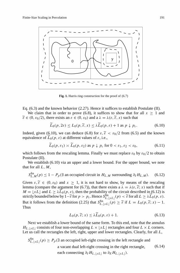
Finite-Size Scaling in Percolation 191
y0
Fig. 1. Harris ring construction for the proof of (6.7)
Eq. (6.3) and the known behavior (2.27). Hence it suffices to establish Postulate (II).We claim that in order to prove (6.8), it suffices to show that for allx ≥ 1 and
ε ∈ (0, ε0/2), there exists anε ∈ (0, ε0) and aλ = λ(ε, ε, x) such that
L0(p,2ε) ≤ L0(p, ε, x) ≤ λL0(p, ε)+ 1 asp ↓ pc. (6.10)
Indeed, given (6.10), we can deduce (6.8) forε, ε < ε0/2 from (6.5) and the knownequivalence ofL0(p, ε) at different values ofε, i.e.,
L0(p, ε1) � L0(p, ε2) asp ↓ pc for 0 < ε1, ε2 < ε0, (6.11)
which follows from the rescaling lemma. Finally we must replaceε0 by ε0/2 to obtainPostulate (II).
We establish (6.10) via an upper and a lower bound. For the upper bound, we notethat for allL,M,
SfinL,M(p) ≤ 1− Pp(∃ an occupied circuit inHL,M surrounding∂IHL,M). (6.12)
Given ε, ε ∈ (0, ε0) and x ≥ 1, it is not hard to show, by means of the rescalinglemma (compare the argument for (6.7)), that there exists aλ = λ(ε, ε; x) such that ifM = �xL andL ≥ λL0(p, ε), then the probability of the circuit described in (6.12) isstrictly bounded below by 1−ε forp > pc. HenceSfin
L,�xL (p) < ε for allL ≥ λL0(p, ε).
But it follows from the definition (2.25) thatSfinL,�xL (p) ≥ ε if L = L0(p, ε; x) − 1.
Thus
L0(p, ε; x) ≤ λL0(p, ε)+ 1. (6.13)
Next we establish a lower bound of the same form. To this end, note that the annulusHL,�xL consists of four non-overlappingL× �xL rectangles and fourL×L corners.Let us call the rectangles the left, right, upper and lower rectangles. Clearly, for allL,
SfinL,�xL (p) ≥ Pp(∃ an occupied left-right crossing in the left rectangle and
a vacant dual left-right crossing in the right rectangle,
each connecting∂IHL,�xL to ∂EHL,�xL ).(6.14)
192 C. Borgs, J. T. Chayes, H. Kesten, J. Spencer
Sincex ≥ 1, the lower bound in (6.14) is only strengthened by requiring that the occupiedcrossing occur in anL× L sub-box of the correspondingL× �xL rectangle and thatthe vacant dual crossing occur in an(L+ 1)× (L− 1) rectangle. By (6.1) this gives
SfinL,�xL (p) ≥ RL,L(1− RL,L) ≥ 1
2(1− RL,L), (6.15)
sincep > pc. Now letL = L0(p, ε; x). It then follows from the definition (2.25) thatSfinL,�xL (p) ≤ ε, so that (6.15) impliesRL,L ≥ 1− (2ε) if L = L0(p, ε; x). Comparing
this with the definition (6.2) forp > pc, we conclude
L0(p, ε; x) ≥ L0(p, 2ε), (6.16)
a lower bound of the desired form."#
6.2. Proof of Postulate (III). Postulate (III) is almost identical to Theorem 1 of [Kes87],except that the latter uses the conditionn ≤ L0(p, ε), whereas Postulate (III) assumesn ≤ L0(p, ε). Thus, to establish Postulate (III), it suffices to show that for allε ∈ (0, ε0),there exists anε ∈ (0, ε0) such that
L0(p, ε) ≤ L0(p, ε). (6.17)
To prove (6.17) we note that by (6.9) we haveL0(p, ε) ≤ λ(ε)L0(p, ε) for p > pcand a suitableλ < ∞. This relation also holds forp < pc, as observed in (6.4).Therefore, it suffices to show that for allp �= pc, λ < ∞, andε ∈ (0, ε0), there existsan ε ∈ (0, ε0) such that
λL0(p, ε) ≤ L0(p, ε). (6.18)
Finally, by (6.3), it suffices to establish (6.18) only forp < pc, and by iteration, toestablish the latter only forλ = 2. To this end, we note that by the Russo-Seymour-Welsh lemma ([Rus78, SW78, Sect. 3.4]), rescaling and the obvious monotonicity ofRL,M , we have
RM,M(p) ≥ f (RL,L(p)) if L ≤ M ≤ 3L, (6.19)
for some functionf on[0,1]which is strictly positive on(0,1].Without loss of generalitywe may takef (ε) ≤ ε. Using the definition (6.2) ofL0(ε, p), we conclude that
RM,M(p) > f (ε) if M ≤ 3L0(p, ε)− 3. (6.20)
As a consequence,
L0(p, f (ε)) ≥ 3L0(ε, p)− 2 ≥ 2L0(p, ε), (6.21)
where we have used thatR1,1(p) ≥ p > ε, and henceL0(p, ε) > 1 in the last step.This establishes (6.18) and hence Postulate (III)."#
Finite-Size Scaling in Percolation 193
6.3. Proof of Postulate (IV). We will establish Postulate (IV) for allp such thatm ≤L0(p) (a somewhat stronger result than the stated postulate atpc). This postulate withρ1 = 2 follows from the claim that for someC1 > 0,
πm(p)
πn(p)≥ C1
(mn
)−1/2if n ≤ m ≤ L0(p). (6.22)
In order to establish (6.22), we assume thatkn ≤ m ≤ (k+ 1)n for some integerk ≥ 1.By (2.12) and monotonicity ofπn,
πm ≥ π(k+1)n ≥ π(k+1)n. (6.23)
Recall the definition (2.9) ofπ(k+1)n and observe that one mechanism to ensure that theorigin is connected to the line atx1 = (k+1)n is to have (1) the origin connected to somepoint in∂Bn(0), (2) some point on∂Bn(0) connected to the line atx1 = (k+1)n, and (3)Harris rings in the annuliBn \Bn/2 andB2n \Bn and a rectangle crossing from (say) theright boundary ofBn/2 to the central quarter of the right boundary ofB2n to “glue” theconnections in (1) and (2) together. Sincen ≤ L0(p), the probability of the third eventis bounded away from zero, uniformly inn (as in (6.7)). Denote the probability of theevent described in (2) above byGn,kn. Equation (6.23) and the Harris-FKG inequalitythen imply that for some constantC2 > 0,
πm ≥ C2πnGn,kn. (6.24)
By an argument almost identical to the proof of Corollary (3.15) in [BK85],kn ≤ L0(p)
impliesGn,kn ≥ C3/√k, whereC3 is a lower bound on the probability of an occupied
crossing of a 2kn × 2kn square. The constantC3 > 0 by virtue of (6.17) and (6.20).(Essentially this same argument is used in [Kes87], Eq. (3.6) and its proof on p. 143.)Thus (6.24) implies the desired bound (6.22)."#
6.4. Proof of Postulate (V). Theorem 3 of [Kes87] gives the second inequality in Pos-tulate (V). Thus it suffices to prove that for a suitable constantD4 and allp > pc,
χcov(p) ≤ D4L20(p)π
2L0(p)
(pc). (6.25)
To this end, we decompose the sum definingχcov(p) (with |v| short for|v|∞ andL0 forL0(p) ):
χcov(p) =∑
|v|≤2L0
Covp(0 ↔ ∞; v ↔ ∞)+∑
|v|>2L0
Covp(0 ↔ ∞; v ↔ ∞). (6.26)
To control the first term, we use the bound (4.4) in Lemma 4.1 and Postulate III toestimate∑
|v|≤2L0
Covp(0 ↔ ∞; v ↔ ∞) ≤∑
|v|≤2L0
Pp{0 ↔ ∞, v ↔ ∞}
≤∑
|v|≤2L0
τ(0, v) ≤∑
|v|≤2L0
π2[|v|/2](p) � L20π
2L0(pc).
(6.27)
194 C. Borgs, J. T. Chayes, H. Kesten, J. Spencer
Next, we bound the second term in (6.26). To this end, letB(w) = BL0(w) be the boxof radiusL0 centered atw. For |v| > 2L0, we have
Covp(0 ↔ ∞; v ↔ ∞) = Covp(0 �↔ ∞; v �↔ ∞)
= Covp(0 �↔ ∞, 0 ↔ ∂B(0); v �↔ ∞, v ↔ ∂B(v))
+ Covp(0 �↔ ∞, 0 ↔ ∂B(0); v �↔ ∂B(v))
+ Covp(0 �↔ ∂B(0); v �↔ ∞, v ↔ ∂B(v))
+ Covp(0 �↔ ∂B(0); v �↔ ∂B(v))
= Covp(0 �↔ ∞, 0 ↔ ∂B(0); v �↔ ∞, v ↔ ∂B(v))
+ 2Covp(0 �↔ ∂B(0); v �↔ ∞, v ↔ ∂B(v)),
(6.28)
where in the last step we have used that Covp(0 �↔ ∂B(0); v �↔ ∂B(v)) = 0 by theindependence of the events{0 �↔ ∂B(0)} and{v �↔ ∂B(v)} whenB(0) andB(v) aredisjoint, and also the symmetry of the roles played by0 andv. Now we bound the secondterm on the right-hand side of (6.28) according to
Covp(0 �↔ ∂B(0); v �↔ ∞, v ↔ ∂B(v))
= Covp(0 �↔ ∂B(0); v �↔ ∞, v ↔ ∂B(v), v ↔ ∂B(0))
+ Covp(0 �↔ ∂B(0); v �↔ ∞, v ↔ ∂B(v), v �↔ ∂B(0))
= Covp(0 �↔ ∂B(0); v �↔ ∞, v ↔ ∂B(0))
= − Covp(0 ↔ ∂B(0); v �↔ ∞, v ↔ ∂B(0))
≤ Pp{0 ↔ ∂B(0)}Pp{v �↔ ∞, v ↔ ∂B(0)},
(6.29)
where we have used that the two events{v �↔ ∞} ∩ {v ↔ ∂B(v)} ∩ {v �↔ ∂B(0)} and0 �↔ ∂B(0) are independent. Using the Harris-FKG inequality and obvious monotonic-ities, the second factor on the right-hand side of (6.29) is in turn bounded accordingto
Prp{v �↔ ∞, v ↔ ∂B(0)}≤ Prp{v ↔ ∂B(0)}
Prp{∃w ∈ ∂B(0) such thatw andv are surrounded by a vacant dual contour}.(6.30)
We now follow a coarse-graining argument along the lines of the proof of Theorem3 in [Kes87] (see (3.12), (3.13) and (2.25) there). Letv = (v1, v2) and for the sakeof argument letv1 = |v| = |v|∞. If there exists a vacant dual contour surroundingw ∈ ∂B(0) andv, then there exists a vacant dual path fromB(0) to someB(v1 + j, v2)
with j ≥ 0. By (2.25) in [Kes87] the probability that such a vacant path exists is at mostC1 exp[−C2|v|/L0]. Together with (6.29) and Postulate III this leads to a bound of
C3π2L0(pc)exp[−C2|v|/L0] (6.31)
for the second term in the right-hand side of (6.28).
Finite-Size Scaling in Percolation 195
Next we bound the first term in the right-hand side of (6.28) by means of the BKinequality as follows:
Prp{0 �↔ ∞, 0 ↔ ∂B(0); v �↔ ∞, v ↔ ∂B(v)}≤ Prp{0 ↔ ∂B(0), v ↔ ∂B(v) and there exist vacant dual contours
C1, C2 surrounding0 andv, respectively}≤ Prp{0 ↔ ∂B(0), v ↔ ∂B(v) and there existedge-disjoint vacant
dual contoursC1, C2 surrounding0 andv, respectively}+ Prp{0 ↔ ∂B(0), v ↔ ∂B(v) and there exist vacant dual contoursC1, C2
surrounding0 andv, respectively, andC1 andC2 have an edge in common}.
By the BK inequality the first term in the right-hand side is no more than
Prp{0 ↔ ∂B(0) and there exists a vacant dual contourC1 which surrounds0}× Prp{v ↔ ∂B(v) and there exists a vacant dual contourC2 which surroundsv}
= Prp{0 �↔ ∞, 0 ↔ ∂B(0)}Prp{v �↔ ∞, v ↔ ∂B(v)}.Therefore,
Covp(0 �↔ ∞, 0 ↔ ∂B(0); v �↔ ∞, v ↔ ∂B(v)}≤ Prp{0 ↔ ∂B(0), v ↔ ∂B(v) and there exist vacant dual contoursC1, C2
surrounding0 andv, respectively, andC1 andC2 have an edge in common}≤ Prp{0 ↔ ∂B(0)}Prp{v ↔ ∂B(v)}Prp{∃ vacant dual contoursC1, C2
surrounding0 andv respectively, andC1 andC2 have an edge in common},(6.32)
where we have used the Harris-FKG inequality and disjointness ofB(0) andB(v) inthe last step. If the two dual contoursC1, C2 in (6.32) have an edge in common, and ifagainv = (v1, v2) with v1 = |v|, thenC1 ∪ C2 contains a vacant dual path from someB(−j1,0) to someB(v1+j2, v2)with j1, j2 ≥ 0. The same argument as used for (6.31)now shows that also the first term in the right-hand side of (6.28) is bounded by (6.31).Finally, then∑
|v|>2L0
Covp(0 ↔ ∞; v ↔ ∞)
≤∑
|v|>2L0
2C3π2L0(pc)exp[−C2|v|/L0] ≤ C(ε)L2
0π2L0(pc). (6.33)
Together with (6.26), (6.27) this yields (6.25)."#
6.5. Proof of Postulate (VI). Postulate (VI) ford = 2 goes back to [Ngu85]. We canalso immediately obtain this from Theorem 2 in [Kes87], which states thatP∞(p) is ofthe same order asπL0(p,ε)
(pc). But by (6.10), (6.11) there exists aλ = λ(ε) ≥ 1 such
thatL0(p, ε) ≤ λL0(p, ε). Therefore, by Postulate (IV)
πL0(p,ε)(pc) ≥ πλL0(p,ε)(pc) ≥ D3λ
−1/ρ1πL0(p,ε)(pc).
196 C. Borgs, J. T. Chayes, H. Kesten, J. Spencer
Combined with Theorem 2 of [Kes87] this gives one inequality of Postulate (VI). In theother direction, it is trivial thatP∞(p) ≤ πL0(p)(p) and furtherπL0(p)(p) � πL0(p)(pc),by Postulate (III). "#
6.6. Proof of Postulate (VII). We shall build a cluster of size at leastks(L0(p)) byconnecting togetherC1k clusters of size at leastC2s(L0(p)) (for suitable constantsC1, C2) in adjacent squares of size 2L0(p). These clusters will be connected by meansof Harris rings.
By Postulate (IV) and Proposition 4.6 (which relies only on Postulate (I)–(IV)) thereexists aσ0 ∈ (0,1] such that forn0 = �σ0L0(p)/2 ,
P≥s(L0(p))(p) ≤ P≥s(n0)(p) ≤ C3πn0(pc);in the first inequality we used that Postulate (IV) implies (5.10), which in turns impliesthats(m) ≥ s(n) if m/n is large enough. In turn, by Postulate (III), the right-hand sidehere is at mostC4πn0(p). It therefore suffices to show that forp < pc and suitableconstantsC5,D6,
P≥ks(L0(p))(p) ≥ C5e−D6kπn0(p). (6.34)
First we use Theorem 3.3 and Lemma 4.4, (4.14). These results show that there existconstantsK0 < ∞ andy0 > 0 such that
Prp{∃ clusterC ⊂ L0(p) with diam(C) ≥ y0L0(p) and|C| ≥ K−10 s(L0(p))}
= Prp{W(1)L0(p)
≥ K−10 s(L0(p))}
− Prp{∃ clusterC ⊂ L0(p) with diam(C) < y0L0(p) and|C| ≥ K−10 s(L0(p))}
≥ 1
2− C1y
−20 exp[−C2(K0y0)
−1] ≥ 1
4,
(6.35)
providedL0(p) ≥ 4/y0. The estimate (6.35) shows that with a probability of at least1/4 there is a cluster with a “large” size and “large” diameter inL0(p). We wish tolocate this large cluster more precisely. In fact we want to show that we may assume thatit crosses a certain rectangle in the first coordinate direction. To this end we note that ifdiam(C) ≥ y0L0(p), then there are two pointsv,w ∈ C so thatwi − vi ≥ y0L0(p) fori = 1 or i = 2. Assume that this holds fori = 1. Then for some−2/y0 ≤ j ≤ 2/y0 theevent
M(p, j) := {∃ clusterC ∈ L0(p) with |C| ≥ K−10 s(L0(p)) that contains
pointsv,w with v1 ≤ jy0L0(p)/2 < (j + 1)y0L0(p)/2 ≤ w1} (6.36)
must occur. Therefore there exists aj0 ∈ [−2/y0,2/y0] for which
Prp{M(p, j0)} ≥ y0
8(y0 + 1). (6.37)
From (6.37) and translation invariance it follows that each of the events
{∃ clusterC0 ∈ [20L0(p), (20+ 2)L0(p))× [−L0(p), L0(p)) with
|C0| ≥ K−10 s(L0(p))and which crosses
[(20+ j0)y0L0(p)/2, (20+ j0 + 1)y0L0(p)/2] × [−L0(p), L0(p))
in the horizontal direction} , 0 ≥ 0,
(6.38)
Finite-Size Scaling in Percolation 197
has probability at leasty0/(8y0 + 8). Let k ≥ 1 be given and taker = 'kK0(. If theevent in (6.38) occurs for0 = 0,1, . . . , r and0 ↔ ∂Bn0(0), and the paths from0 to∂Bn0(0)and the horizontal crossings of[(20+j0)y0L0(p)/2, (20+j0+1)y0L0(p)/2]×[−L0(p), L0(p)) ,0 ≤ 0 ≤ r are all connected by Harris rings, then the cluster of theorigin has size at leastrK−1
0 s(L0(p)) ≥ ks(L0(p)). The Harris-FKG inequality nowshows that
P≥ks(L0(p))(p) ≥ πn0(p)C6[C6y0
8(y0 + 1)]r .
This proves (6.34) with
D6 = log8(y0 + 1)(K0 + 1)
C6y0,
and Postulate (VII) follows for allp < pc with L0(p) ≥ 4/y0. If L0(p) < 4/y0, the
postulate follows from the trivial boundP≥ks(L0(p)) ≥ pks(L0(p)) ≥ p64y−20 k.
"#
7. Proof of Theorem 3.7
In this section, we introduce Postulate (VII alt), which is slightly stronger than Postulate(VII), and prove Theorem 3.7. To state the Postulate (VII alt), we need some notation.Fork ≥ 1, let[k]d = {1, . . . , k}d . Given an integerk ≥ 1, and a choice of verticesv( j)in ( j) := 2jL0(p) + �L0(p)/4 , j ∈ [k]d , we define sets( j) = 2jL0(p) + L0(p)
and
F =⋃
j∈[k]d( j),
as well as events
G( j) = G(j; x) = {|C( j)(v( j))| ≥ xs(L0(p))},Gk = Gk(x) =
⋂j∈[k]d
G(j; x),
H( j) = {v( j) ↔ v(j ± ei) in F, 1 ≤ i ≤ d},where theith component ofj ± ei equalsji ± 1. We also define
Hk = {all v( j) with j ∈ [k]d are connected inF} =⋂
2≤ji≤k−11≤i≤d
H( j).
Postulate (VII alt). For all 0< x ≤ 1 there exists a constantD7 = D7(x) > 0 suchthat
Prp{Hk | Gk(x)} ≥ Dkd
7 (7.1)
for all ζ0 ≤ p < pc, k ≥ 1 and all choices ofv( j), j ∈ [k]d . We remind the reader thatζ0 is some arbitrary number in(0, pc).
198 C. Borgs, J. T. Chayes, H. Kesten, J. Spencer
Note that there arekd choices forj ∈ [k]d . Condition (7.1) therefore roughly speakingsays that the conditional probability ofH( j), given that|C(v( j))| ≥ xs(L0(p)) and each|C(v( j ± ei))| ≥ xs(L0(p)), is at leastD7. Or still more intuitively, “clusters of sizeof orders(L0(p)) and a distance of orderL0(p)) apart have a reasonable conditionalprobability of being connected." We also mention that (7.1) is actually not needed forall x ∈ (0,1], but only for one fixed value ofx for whichPrp{G( j)} ≥ C1πL0(p)(pc)
for some constantC1 > 0, independent ofp < pc. Suchx andC1 can be shown to existby means of the bound (5.40) which follows from Proposition 5.3.
7.1. Proof of Theorem 3.7i. In this subsection we always assume Postulates (I)–(IV)andζ0 ≤ p < pc. For brevity we write in many placesL for L0(p) and for L0(p).In Steps i–v we also use Postulate (VII alt), but we only shall use that (7.1) is valid for0 < x ≤ x0 for somex0 > 0. The value ofx0 is irrelevant. All constants in this sectionare independent ofk.
Step i. There exists anx ∈ (0,1] and a constantC2 > 0 such that uniformly forv( j) ∈ ( j) = 2 jL0(p)+�L0(p)/4 ,
Prp{G( j)} ≥ C2πL(pc). (7.2)
To prove (7.2) we use the relation (5.3) between the distribution ofW(1) andP≥s . For
r ≥ 1 and any 0< C1 < ∞, we get
Prp{W(1)r
≥ C1s(r)} ≤∑v∈r
∑s≥C1s(r)
1
sP rp{|Cr (v)| = s}
≤ |r |C1s(r)
supv∈r
P rp{|Cr (v)| ≥ C1s(r)}.(7.3)
On the other hand, by (5.10),s(m) ≥ s(r) and hence
Prp{W(1)r
≥ C1s(r)} ≥ Prp{W(1)r
≥ s(m)} (7.4)
wheneverm ≥ r(C1/D3)2/d . Settingr = �L0(p)/4 ,m = r'(C1/D3)
2/d(, and choos-ing C1 > 0 small enough to guarantee that'(C1/D3)
2/d(σ (1)(1/4,1/2) ≤ 1, whereσ (1)(λ, δ) is the constant introduced before (5.40), we can now use the bound (5.40).Combined with (7.4) we getPrp{W(1)
r≥ C1s(r)} ≥ 1/2. Using (7.3), we therefore
conclude that there exists a constantC3 > 0 and aw0 ∈ r such that
Prp{|Cr (w0)| ≥ C1s(r)} ≥ 12C2πr(p) ≥ C3πr(pc), (7.5)
where we used Postulate (III) in the last step. Now for anyv ∈ r, r shifted byv−w0is contained in3r ⊂ . Therefore for allv ∈ r = �L0(p)/4 and sufficiently smallC4,
Prp{|C(v)| ≥ C4s(L)} ≥ Prp{|Cr (w0)| ≥ C1s(r)} ≥ C3πr(pc) ≥ C2πL(pc).
(7.6)
This proves (7.2) forj = 0 andx = C4 ∧ 1. But then it clearly holds for allj bytranslation and for all 0< x ≤ C4 ∧ 1.
Finite-Size Scaling in Percolation 199
Step ii. Now fix k and for brevity writeM = kd . LetC2 andC4 be such that (7.6) holds.Also fix x = C4 ∧ 1∧ x0 and takeD7 = D7(x). It is useful to indicate the choice of thev( j)more explicitly in our notation. With some abuse of notation we denote the possiblevalues ofj by 1, . . . ,M, and we occasionaly writeGk(v(1), . . . , v(M)) instead ofGk,and similarly forHk(v(1), . . . , v(M)).
We have defined the( j) such that they are disjoint. Consequently, for any choiceof v( j) in ( j), we have by (7.2)
Prp{Gk(v(1), . . . , v(M))} =∏
j
Prp{G( j)} ≥ [C2πL(pc)]M,
and then by Postulate (VII alt)
Prp{Gk(v(1), . . . , v(M)) ∩Hk(v(1), . . . , v(M))} ≥ [D7C2πL(pc)]M. (7.7)
We sum this over allv( j) ∈ ( j) for j �= 1. We indicate this sum by∑
(k). We thereforehave for some constantsC5, C6,∑
(k)P rp{Gk(v(1), . . . , v(M)) ∩Hk(v(1), . . . , v(M))
≥ [D7C2πL(pc)]M [2�L0(p)/4 ]M−1 ≥ C5πL(pc)[C6s(L)]M−1.(7.8)
Step iii. We next work on an upper bound for the left-hand side of (7.8). To this endwe note that on the eventGk ∩ Hk, v( j) is connected tov(1) and therefore to∂( j)wheneverj �= 1. We therefore define
V ( j) = number ofv ∈ ( j) which are connected to∂( j).
We further define
Ik = Ik(v(1)) = I [|CF(v(1))| ≥ Mxs(L)]. (7.9)
Clearly, on the eventGk(v(1), . . . , v(M)) ∩Hk(v(1), . . . , v(M)), it holds that
|CF(v(1))| ≥∑
j
|C( j)(v( j))| ≥ Mxs(L) andv( j) ↔ ∂( j),
and therefore∑(k)P rp{Gk(v(1), . . . , v(M)) ∩Hk(v(1), . . . , v(M))}
≤ Ep{Ik(v(1))I [v(1) ↔ ∂(1)]∏j�=1
V ( j)}. (7.10)
We continue this inequality. For anyγ ≥ 0 the right-hand side of (7.10) is at most
eγM [s(L)]M−1Ep{Ik(v(1))}+ Ep
{Ik(v(1))I [v(1) ↔ ∂(1)]
∏j�=1
V ( j);∏j�=1
V ( j) ≥ eγM [s(L)]M−1}
≤ eγM [s(L)]M−1Ep{Ik(v(1))}+ e−γM [s(L)]−M+1Ep
{I [v(1) ↔ ∂(1)]
∏j�=1
V 2( j)}.
200 C. Borgs, J. T. Chayes, H. Kesten, J. Spencer
Finally we observe that theV ( j) are independent among each other and ofI [v(1) ↔∂(1)], because the( j) are disjoint. Moreover, for eachj,
Ep{V 2( j)} ≤ C7s2(L),
by virtue of (4.6). Therefore
Ep{I [v(1) ↔ ∂(1)]∏j�=1
V 2( j)} = Prp{v(1) ↔ ∂(1)}∏j�=1
Ep{V 2( j)}
≤ π�L/2 (pc)[C7s(L)]2M−2.
Combining these estimates gives∑(k)P rp{Gk(v(1), . . . , v(M)) ∩Hk(v(1), . . . , v(M))}
≤ eγM [s(L)]M−1Ep{Ik(v(1))} + e−γM [s(L)]−M+1π�L/2 (pc)[C7s(L)]2M−2.
(7.11)
Step iv. In this step we complete the deduction of Postulate (VII) from Postulates (I)–(V)and Postulate (VII alt). From (7.8)–(7.11) we obtain (by means of Postulate (IV))
eγM [s(L)]M−1Ep{Ik(v(1))}≥ C5πL(pc)
{[C6s(L)]M−1 − e−γM [s(L)]−M+1(C5D3)−121+1/ρ1[C7s(L)]2M−2}.
Choosingγ so large that
e−γ < C6C−27 ∧
[1
4C5D32−1/ρ1
],
we find that
Ep{Ik(v(1))} ≥ πL(pc)e−γM 1
2C5C
M−16 . (7.12)
Since, by (7.9), the left-hand side is no more than
P≥Mxs(L)(p),
and, by (4.20),πL(pc) ≥ C−12 P≥s(L)(pc) ≥ C−1
2 P≥s(L)(p), we obtain Postulate (VII).
Step v. Even though we finished the deduction of Postulate (VII), we point out here thathad we summed overv(1) as well, then the derivation given above would have resultedin
Prp{W(1)kL
≥ C2Ms(L)}= Prp{∃ a cluster in
⋃j
( j) of size ≥ C2Ms(L)}
≥ C9e−γMCM
6 .
(7.13)
This is basically the estimate (5.83) and we can deduce the lower bound in Theorem3.5 almost immediately from (7.13) without repeating most of its proof from Postulate(VII).
Finite-Size Scaling in Percolation 201
Also (7.13) can be used to derive the desired counterpart to (3.14), namely, for eachfixedK andi,
lim supPpn{ W
(i)n
Epn{W(i)n
}≤ K
}< 1, (7.14)
whenpn is inside the scaling window, i.e., when (3.5) holds. To see (7.14) fori = 1, fixsome largeK. Then choosek such that for large n,
KEpn{W(1)n
} ≤ C2C−11
(k
2
)1/ρ2
s(n) andkL0(p) > 2n, (7.15)
with C1 as in (4.17). Such ak exists becauseEpn{W(1)n
} ands(n) are of the same orderby Theorem 3.1 i) andpn is inside the scaling window. Finally choosep′
n ≤ (pn ∧ pc)
such that
n ≤ kL0(p′n) ≤ 2n.
This can be done by virtue of (2.29). Lemma 4.5 then shows that
C2kds(L0(p
′n)) ≥ C2C
−11
(k
2
)1/ρ2
s(n) ≥ KEpn{W(1)n
} (see (7.15)).
Finally, then, by (7.13) forp = p′n,
Ppn{W(1)n
≥ KEpn{W(1)n
}} ≥ Ppn{W(1)n
≥ C2kds(L0(p
′n))}
≥ Pp′n{W(1)
n≥ C2k
ds(L0(p′n))} ≥ C9e
−γ kdCkd
6 > 0.
This proves (7.14) fori = 1. For generali a little extra work is needed as in the last fewlines of the proof of Theorem 3.5."#
7.2. Proof of Theorem 3.7ii. We briefly indicate how to derive Postulate (VII alt) indimension 2. We first show that (7.1) holds whenx is sufficiently small. In fact, ifK0, y0and j0 are the constants for which (6.35)–(6.37) hold, then this argument works forx ≤ [K0]−1. With M(p, j) as in (6.36), we have by a Harris ring construction that forsuitable constantsC1, C2 > 0 and allv( j) ∈ ( j),
Prp{∃ clusterC ∈ L0(p) which containsv( j) and points
v,w with v1 ≤ j0y0L0(p)/2 < (j0 + 1)y0L0(p)/2 ≤ w1
and with|C| ≥ K−10 s(L0(p))}
≥ C1Prp{M(p, j0)}Prp{v( j) ↔ ∂BL0(p)(v( j)} ≥ C1y0
8(y0 + 1)πL0(p)(p)
≥ C2πL0(p)(pc).
(7.16)
On the other hand, by definition ofG( j),
Prp{G( j)} ≤ P≥xs(L0(p))(p).
202 C. Borgs, J. T. Chayes, H. Kesten, J. Spencer
Using the bound
P≥s(p) ≤ πn(p)+ 1
s
n∑m=1
|∂Bm|[π�m/2 (p)
]2,
proven in [BCKS98], Eq. (4.20), one easily shows that there is a constantC10 =C10(x) < ∞ such that
P≥xs(L0(p))(p) ≤ C10πL0(p)(pc).
Since theG( j) for differentj depend on disjoint regions, they are independent, and
Prp{Gk} ≤ [P≥xs(L0(p))(p)]k2 ≤ [C10πL0(p)(pc)]k
2. (7.17)
Finally, denote the event in the left-hand side of (7.16) byK( j), that is
K( j) = ∃ clusterC ∈ L0(p) which containsv( j) and points
v,w with v1 ≤ j0y0L0(p)/2 < (j0 + 1)y0L0(p)/2 ≤ w1
and with|C| ≥ K−10 s(L0(p))}.
Note thatK( j) impliesG( j)whenx ≤ [K0]−1. Therefore another Harris ring construc-tion shows that for some constantC11 > 0,
Prp{Gk ∩Hk} ≥ Ck2
11Prp{K( j) for all 1 ≤ ji ≤ k, i = 1,2}≥ Ck2
11[C2πL0(p)(pc)]k2,
by virtue of (7.16) and the Harris–FKG inequality. Comparing this with (7.17), we seethat
Prp{Gk ∩Hk} ≥ [C11C2/C10]k2Prp{Gk}.
This completes the proof of (7.1) whenx ≤ [K0]−1.For our purposes (7.1) for 0< x ≤ [K0]−1 is actually good enough, but it is not hard
to obtain (7.1) for general 0< x ≤ 1 now. In fact, we can apply the same argument asabove, provided we first prove the following strengthening of (7.16) for some constantC12 > 0:
Prp{∃ clusterC ∈ L0(p) which containsv( j) and points
v,w with v1 ≤ j0y0L0(p)/2 < (j0 + 1)y0L0(p)/2 ≤ w1
and with|C| ≥ s(L0(p))}≥ C12πL0(p)(pc).
(7.18)
But (7.18) can be derived exactly as (7.16) from an analogue of (6.37) if we start from
Prp{∃ clusterC ∈ L0(p) with diam(C) ≥ y0L0(p) and|C| ≥ s(L0(p))}≥ Prp{W(1)
L0(p)≥ s(L0(p))}
− Prp{∃ clusterC ⊂ L0(p) with diam(C) ≤ y0L0(p) but |C| ≥ s(L0(p))}≥ Prp{W(1)
L0(p)≥ s(L0(p))} − C1y
−20 exp[−C3y
−10 ]
≥ C13 > 0,(7.19)
Finite-Size Scaling in Percolation 203
which is valid for sufficiently smally0 > 0 and some constantC13 > 0. Equation (7.19)is the analogue of (6.35) with[K0]−1 replaced by 1. The reason why we can prove thisnow, but could not take[K0]−1 = 1 in (6.35) to begin with, is that we first needed toshow thatPrp{W(1)
L0(p)≥ s(L0(p))} is bounded away from 0. But this is now available
to us from (7.14). As we pointed out before (7.14) only needs (7.1) for 0< x ≤ x0 forsomex0 > 0, and this we just derived."#
Acknowledgements. The authors wish to thank the Forschungsinstitut of the ETH in Zürich and the Institutefor Advanced Study in Princeton for their hospitality and partial support of the research in this paper. Theauthors are also grateful for partial support from other sources: C.B. was supported by the Commission ofthe European Union under the grant CHRX-CT93-0411, J.T.C. by NSF grant DMS-9403842, and H.K. by anNSF grant to Cornell University.
References
[ACCFR83] Aizenman, M., Chayes, J.T., Chayes, L., Fröhlich, J. and Russo, L.: On a sharp transition fromarea law to perimeter law in a system of random surfaces. Commun. Math. Phys.92, 19–69(1983)
[Aiz97] Aizenman, M.: On the number of incipient spanning clusters. Nucl. Phys. B[FS]485, 551–582(1997)
[Ald97] Aldous, D.: Brownian excursions, critical random graphs and the multiplicative coalescent.Ann. Probab.25, 812–854 (1997)
[Ale96] Alexander, K.: Private communication (1996)[AN84] Aizenman, M. and Newman, C.M.: Tree graph inequalities and critical behavior in percolation-
models. J. Stat. Phys.36, 107–143 (1984)[AS92] Alon, N. and Spencer, J.:The Probabilistic Method. New York: Wiley Interscience, 1992[BBCK98] Bollobás, B., Borgs, C., Chayes, J.T. and Kim, J.-H.: Unpublished (1998)[BCKS98] Borgs, C., Chayes, J.T., Kesten, H. and Spencer, J.: Uniform boundedness of critical crossing
probabilities implies hyperscaling. Rand. Struc. Alg.15, 368–413 (1999)[BC96] Borgs, C. and Chayes, J.T.: On the covariance matrix of the Potts model: A random cluster
analysis. J. Stat. Phys.82, 1235–1297 (1996)[BI92-1] Borgs, C. and Imbrie, J.: Finite-size scaling and surface tension from effective one-dimensional
systems. Commun. Math. Phys.145, 235–280 (1992)[BI92-2] Borgs, C. and Imbrie, J.: Crossover finite-size scaling at first order transitions. J. Stat. Phys.69,
487–537 (1992)[BK85] van den Berg, J. and Kesten, H.: Inequalities with applications to percolation and reliability. J.
Appl. Probab.22, 556–569 (1985)[BoK90] Borgs, C. and Kotecký, R.:A rigorous theory of finite-size scaling at first-order phase transitions.
J. Stat. Phys.61, 79–110 (1990)[Bol84] Bollobás, B.: The evolution of random graphs. Trans. Am. Math. Soc.286, 257–274 (1984)[Bol85] Bollobás, B.:Random Graphs. London: Academic Press, 1985[CC86] Chayes, J.T. and Chayes, L.: Percolation and random media. In:Random Systems and Gauge
Theories, Les Houches, Session XLIII, eds K. Osterwalder and R. Stora Amsterdam: Elsevier,1986, pp. 1001–1142
[CC87] Chayes, J.T. and Chayes, L.: On the upper critical dimension in Bernoulli Percolation. Commun.Math. Phys.113, 27–48 (1987)
[CCD87] Chayes, J.T., Chayes, L. and Durrett, R.: Inhomogeneous percolation problems and incipientinfinite clusters. J. Phys. A: Math. Gen.20, 1521–1530 (1987)
[CCF85] Chayes, J.T., Chayes, L. and Fröhlich, J.: The low-temperature behavior of disordered magnets.Commun. Math. Phys.100, 399–437 (1985)
[CCFS86] Chayes, J.T., Chayes, L., Fisher, D. and Spencer, T.: Finite-size scaling and correlation lengthsfor disordered systems. Phys. Rev. Lett.57, 2999-3002 (1986)
[CCGKS89] Chayes, J.T., Chayes, L., Grimmett, G.R., Kesten, H. and Schonmann, R.H.: The correlationlength for the high-density phase of Bernoulli percolation. Ann. Probab.17, 1277–1302 (1989)
[Cha98] Chayes, J.T.: Finite-size scaling in percolation. Doc. Math. J. DMV, Extra Volume ICM III113–122, (1998)
[CPS96] Chayes, J.T., Puha, A.L. and Sweet, T.: Independent and dependent percolation. In:IAS-ParkCity Mathematics Series, Vol. 6 Probability Theory and Applications (Princeton, NJ, 1996),Providence, RI: AMS, 1999, pp. 49–166
204 C. Borgs, J. T. Chayes, H. Kesten, J. Spencer
[Con85] Coniglio,A.: Shapes, surfaces and interfaces in percolation clusters. In:Proc. Les Houches Con-ference on Physics of Finely Divided Matter, eds M. Daoud and N. Boccara Berlin–Heidelberg–New York: Springer-Verlag, 1985, pp. 84–109
[ER59] Erdos, P. and Rényi, A.: On random graphs I. Publ. Math. (Debrecen)6, 290–297 (1959)[ER60] Erdos, P. and Rényi, A.: On the evolution of random graphs. Magy. Tud. Akad. Mat. Kut. Intéz.
Közl. 5, 17–61 (1960)[GM90] Grimmett, G. and Marstrand, J.M.: The supercritical phase of percolation is well behaved. Proc.
Roy. Soc. London Ser. A430, 439–457 (1990)[Gri99] Grimmett, G.:Percolation. 2nd edition, New York: Springer-Verlag, 1999[Ham57] Hammersley: Percolation processes. Lower bounds for the critical probability. Ann. Math.
Statist.28, 790–795 (1957)[Har01] Hara, T.: Critical two-point functions for nearest-neighbour high-dimensional self-avoiding
walk and percolation. Preprint in preparation[HHS01] Hara, T., van der Hofstad, R. and Slade, G.: Critical two-point functions and the lace expansion
for spread-out high-dimensional percolation and related models. Preprint, (2001)[Har60] Harris, T.E.: A lower bound for the critical probability in a certain percolation process. Proc.
Cambridge Philos. Soc.56, 13–20 (1960)[Jar00] Járai, A.: Incipient infinite percolation clusters in 2D. Preprint (2000)[JKLP93] Janson, S., Knuth, D.E., Łuczak, T. and Pittel, B.: The birth of the giant component. Random
Struc. Alg.4, 233–358 (1993)[Kes82] Kesten, H.:Percolation Theory for Mathematicians. Boston: Birkhäuser, 1982[Kes86] Kesten, H. : The incipient infinite cluster in two-dimensional percolation. Probab. Theory Rel.
Fields73, 369–394 (1986)[Kes87] Kesten, H.: Scaling relations for 2D-percolation. Commun. Math. Phys.109, 109–156 (1987)[Luc90] Łuczak, T.: Component behavior near the critical point of the random graph process. Rand.
Struc. Alg.1, 287–310 (1990)[Ngu85] Nguyen, B.G.: Correlation lengths for percolation processes. PhD thesis, UCLA (1985)[Ngu88] Nguyen, B.G.: Typical cluster size for two-dimensional percolation processes. J. Stat. Phys.50,
715–726 (1988)[Rus78] Russo, L.: A note on percolation. Z. Wahrsch. verw. Geb.43, 39–48 (1978)[SmW78] Smythe, R.T. and Wierman, J.C.:First-Passage Percolation on the Square Lattice. Berlin-
Heidelberg: Springer-Verlag, 1978[SW78] Seymour, P.D. and Welsh, D.J.A.: Percolation probabilities on the square lattice. Ann. Discrete
Math.3, 227–245 (1978)
Communicated by M. Aizenman
![Percolation on Fuchsian groups - University of Chicagolalley/Papers/percolation.pdf · the percolation regime p >/~c the infinite cluster is unique [3]. The purpose of this paper](https://img.pdfslide.net/doc/110x75/5fd26bed6ae80e5b09540038/percolation-on-fuchsian-groups-university-of-lalleypaperspercolationpdf-the.jpg)