The blue and green colors are actually the same

http://blogs.discovermagazine.com/badastronomy/2009/06/24/the-blue-and-the-green/

How is it that a 4MP image can be compressed to a few hundred KB without a noticeable change?

Compression

Lossy Image Compression (JPEG)

Block-based Discrete Cosine Transform (DCT)

Slides: Efros

Using DCT in JPEG

• The first coefficient B(0,0) is the DC component, the average intensity

• The top-left coeffs represent low frequencies, the bottom right – high frequencies

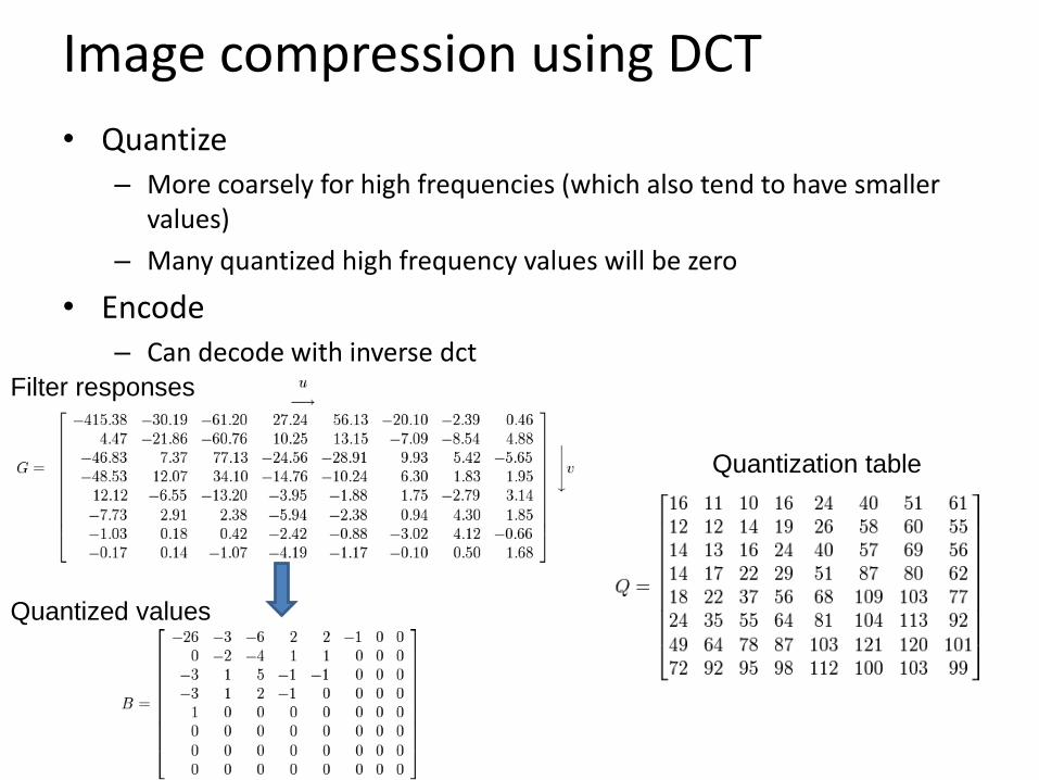
Image compression using DCT

• Quantize – More coarsely for high frequencies (which also tend to have smaller

values)

– Many quantized high frequency values will be zero

• Encode– Can decode with inverse dct

Quantization table

Filter responses

Quantized values

JPEG Compression Summary

1. Convert image to YCrCb

2. Subsample color by factor of 2– People have bad resolution for color

3. Split into blocks (8x8, typically), subtract 128

4. For each blocka. Compute DCT coefficients

b. Coarsely quantize• Many high frequency components will become zero

c. Encode (with run length encoding and then Huffman coding for leftovers)

http://en.wikipedia.org/wiki/YCbCr

http://en.wikipedia.org/wiki/JPEG

Why do we get different, distance-dependent interpretations of hybrid images?

?

• Early processing in humans filters for various orientations and scales of frequency

• Perceptual cues in the mid-high frequencies dominate perception

• When we see an image from far away, we are effectively subsampling it

Early Visual Processing: Multi-scale edge and blob filters

Clues from Human Perception

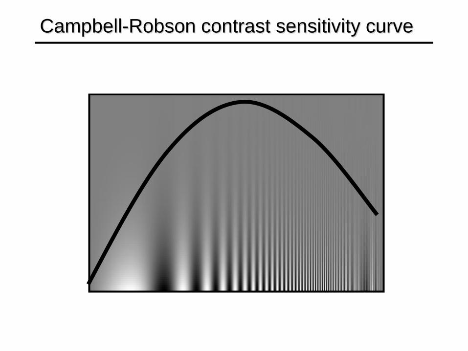
Campbell-Robson contrast sensitivity curve

Hybrid Image in FFT

Hybrid Image Low-passed Image High-passed Image

0 0 0 0 0 0 0 0 0 0

0 0 0 0 0 0 0 0 0 0

0 0 0 90 90 90 90 90 0 0

0 0 0 90 90 90 90 90 0 0

0 0 0 90 90 90 90 90 0 0

0 0 0 90 0 90 90 90 0 0

0 0 0 90 90 90 90 90 0 0

0 0 0 0 0 0 0 0 0 0

0 0 90 0 0 0 0 0 0 0

0 0 0 0 0 0 0 0 0 0

0

0 0 0 0 0 0 0 0 0 0

0 0 0 0 0 0 0 0 0 0

0 0 0 90 90 90 90 90 0 0

0 0 0 90 90 90 90 90 0 0

0 0 0 90 90 90 90 90 0 0

0 0 0 90 0 90 90 90 0 0

0 0 0 90 90 90 90 90 0 0

0 0 0 0 0 0 0 0 0 0

0 0 90 0 0 0 0 0 0 0

0 0 0 0 0 0 0 0 0 0

Credit: S. Seitz

],[],[],[,

lnkmglkfnmhlk

[.,.]h[.,.]f

Review: Image filtering

111

111

111

],[g

0 0 0 0 0 0 0 0 0 0

0 0 0 0 0 0 0 0 0 0

0 0 0 90 90 90 90 90 0 0

0 0 0 90 90 90 90 90 0 0

0 0 0 90 90 90 90 90 0 0

0 0 0 90 0 90 90 90 0 0

0 0 0 90 90 90 90 90 0 0

0 0 0 0 0 0 0 0 0 0

0 0 90 0 0 0 0 0 0 0

0 0 0 0 0 0 0 0 0 0

0 10

0 0 0 0 0 0 0 0 0 0

0 0 0 0 0 0 0 0 0 0

0 0 0 90 90 90 90 90 0 0

0 0 0 90 90 90 90 90 0 0

0 0 0 90 90 90 90 90 0 0

0 0 0 90 0 90 90 90 0 0

0 0 0 90 90 90 90 90 0 0

0 0 0 0 0 0 0 0 0 0

0 0 90 0 0 0 0 0 0 0

0 0 0 0 0 0 0 0 0 0

],[],[],[,

lnkmglkfnmhlk

[.,.]h[.,.]f

Image filtering

111

111

111

],[g

Credit: S. Seitz

0 0 0 0 0 0 0 0 0 0

0 0 0 0 0 0 0 0 0 0

0 0 0 90 90 90 90 90 0 0

0 0 0 90 90 90 90 90 0 0

0 0 0 90 90 90 90 90 0 0

0 0 0 90 0 90 90 90 0 0

0 0 0 90 90 90 90 90 0 0

0 0 0 0 0 0 0 0 0 0

0 0 90 0 0 0 0 0 0 0

0 0 0 0 0 0 0 0 0 0

0 10 20

0 0 0 0 0 0 0 0 0 0

0 0 0 0 0 0 0 0 0 0

0 0 0 90 90 90 90 90 0 0

0 0 0 90 90 90 90 90 0 0

0 0 0 90 90 90 90 90 0 0

0 0 0 90 0 90 90 90 0 0

0 0 0 90 90 90 90 90 0 0

0 0 0 0 0 0 0 0 0 0

0 0 90 0 0 0 0 0 0 0

0 0 0 0 0 0 0 0 0 0

],[],[],[,

lnkmglkfnmhlk

[.,.]h[.,.]f

Image filtering

111

111

111

],[g

Credit: S. Seitz

Filtering in spatial domain-101

-202

-101

* =

Filtering in frequency domain

FFT

FFT

Inverse FFT

=

Review of Filtering

• Filtering in frequency domain

– Can be faster than filtering in spatial domain (for large filters)

– Can help understand effect of filter

– Algorithm:

1. Convert image and filter to fft (fft2 in matlab)

2. Pointwise-multiply ffts

3. Convert result to spatial domain with ifft2

Review of Filtering

• Linear filters for basic processing

– Edge filter (high-pass)

–Gaussian filter (low-pass)

FFT of Gaussian

[-1 1]

FFT of Gradient Filter

Gaussian

Things to Remember

• Sometimes it makes sense to think of images and filtering in the frequency domain– Fourier analysis

• Can be faster to filter using FFT for large images (N logN vs. N2 for auto-correlation)

• Images are mostly smooth– Basis for compression

• Remember to low-pass before sampling

Previous Lectures

• We’ve now touched on the first three chapters of Szeliski.

– 1. Introduction

– 2. Image Formation

– 3. Image Processing

• Now we’re moving on to

– 4. Feature Detection and Matching

– Multiple views and motion (7, 8, 11)

Edge / Boundary Detection

Computer Vision

James Hays

Many slides from Lana Lazebnik, Steve Seitz, David Forsyth, David Lowe, Fei-Fei Li, and Derek Hoiem

Szeliski 4.2

Edge detection

• Goal: Identify sudden changes (discontinuities) in an image– Intuitively, most semantic and

shape information from the image can be encoded in the edges

– More compact than pixels

• Ideal: artist’s line drawing (but artist is also using object-level knowledge)

Source: D. Lowe

Why do we care about edges?

• Extract information, recognize objects

• Recover geometry and viewpoint

Vanishingpoint

Vanishingline

Vanishingpoint

Vertical vanishingpoint

(at infinity)

Origin of Edges

• Edges are caused by a variety of factors

depth discontinuity

surface color discontinuity

illumination discontinuity

surface normal discontinuity

Source: Steve Seitz

Closeup of edges

Source: D. Hoiem

Closeup of edges

Source: D. Hoiem

Closeup of edges

Source: D. Hoiem

Closeup of edges

Source: D. Hoiem

Characterizing edges

• An edge is a place of rapid change in the image intensity function

imageintensity function

(along horizontal scanline) first derivative

edges correspond to

extrema of derivative

Intensity profile

Source: D. Hoiem

With a little Gaussian noise

Gradient

Source: D. Hoiem

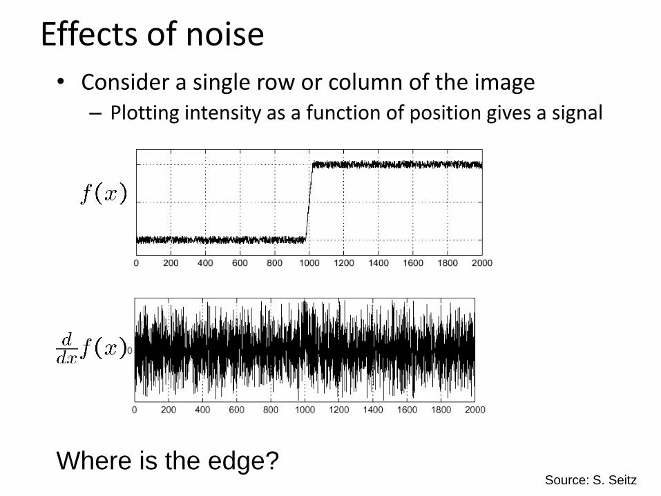
Effects of noise• Consider a single row or column of the image

– Plotting intensity as a function of position gives a signal

Where is the edge?Source: S. Seitz

Effects of noise

• Difference filters respond strongly to noise

– Image noise results in pixels that look very different from their neighbors

– Generally, the larger the noise the stronger the response

• What can we do about it?

Source: D. Forsyth

Solution: smooth first

• To find edges, look for peaks in )( gfdx

d

f

g

f * g

)( gfdx

d

Source: S. Seitz

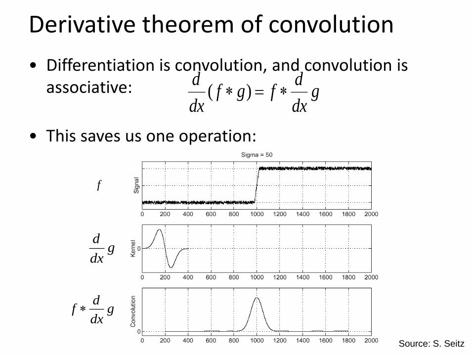
• Differentiation is convolution, and convolution is associative:

• This saves us one operation:

gdx

dfgf

dx

d )(

Derivative theorem of convolution

gdx

df

f

gdx

d

Source: S. Seitz

Derivative of Gaussian filter

* [1 -1] =

• Smoothed derivative removes noise, but blurs edge. Also finds edges at different “scales”.

1 pixel 3 pixels 7 pixels

Tradeoff between smoothing and localization

Source: D. Forsyth

Designing an edge detector• Criteria for a good edge detector:

– Good detection: the optimal detector should find all real edges, ignoring noise or other artifacts

– Good localization• the edges detected must be as close as possible to

the true edges• the detector must return one point only for each

true edge point

• Cues of edge detection– Differences in color, intensity, or texture across the

boundary– Continuity and closure– High-level knowledge

Source: L. Fei-Fei

Canny edge detector

• This is probably the most widely used edge detector in computer vision

• Theoretical model: step-edges corrupted by additive Gaussian noise

• Canny has shown that the first derivative of the Gaussian closely approximates the operator that optimizes the product of signal-to-noise ratio and localization

J. Canny, A Computational Approach To Edge Detection, IEEE

Trans. Pattern Analysis and Machine Intelligence, 8:679-714, 1986.

Source: L. Fei-Fei

27,000 citations!

Example

original image (Lena)

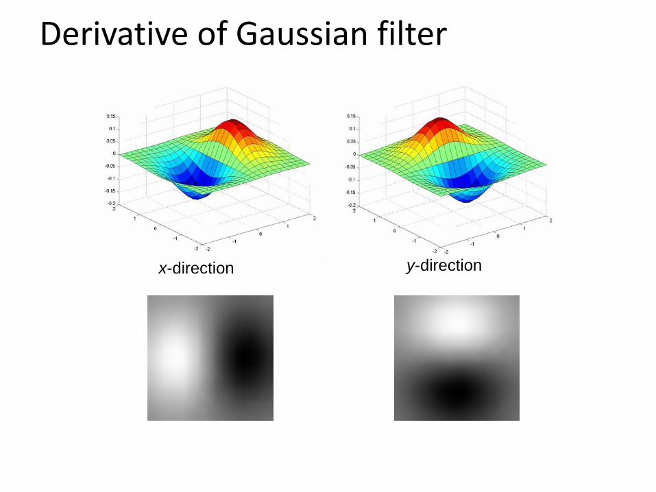
Derivative of Gaussian filter

x-direction y-direction

Compute Gradients (DoG)

X-Derivative of Gaussian Y-Derivative of Gaussian Gradient Magnitude

Get Orientation at Each Pixel

• Threshold at minimum level

• Get orientation

theta = atan2(gy, gx)

Non-maximum suppression for each orientation

At q, we have a

maximum if the

value is larger than

those at both p and

at r. Interpolate to

get these values.

Source: D. Forsyth

Sidebar: Interpolation options

• imx2 = imresize(im, 2, interpolation_type)

• ‘nearest’ – Copy value from nearest known– Very fast but creates blocky edges

• ‘bilinear’– Weighted average from four nearest known

pixels– Fast and reasonable results

• ‘bicubic’ (default)– Non-linear smoothing over larger area (4x4)– Slower, visually appealing, may create

negative pixel values

Examples from http://en.wikipedia.org/wiki/Bicubic_interpolation

Before Non-max Suppression

After non-max suppression

Hysteresis thresholding

• Threshold at low/high levels to get weak/strong edge pixels

• Do connected components, starting from strong edge pixels

Hysteresis thresholding

• Check that maximum value of gradient value is sufficiently large

– drop-outs? use hysteresis

• use a high threshold to start edge curves and a low threshold to continue them.

Source: S. Seitz

Final Canny Edges

Canny edge detector

1. Filter image with x, y derivatives of Gaussian

2. Find magnitude and orientation of gradient

3. Non-maximum suppression:

– Thin multi-pixel wide “ridges” down to single pixel width

4. Thresholding and linking (hysteresis):

– Define two thresholds: low and high

– Use the high threshold to start edge curves and the low threshold to continue them

• MATLAB: edge(image, ‘canny’)

Source: D. Lowe, L. Fei-Fei

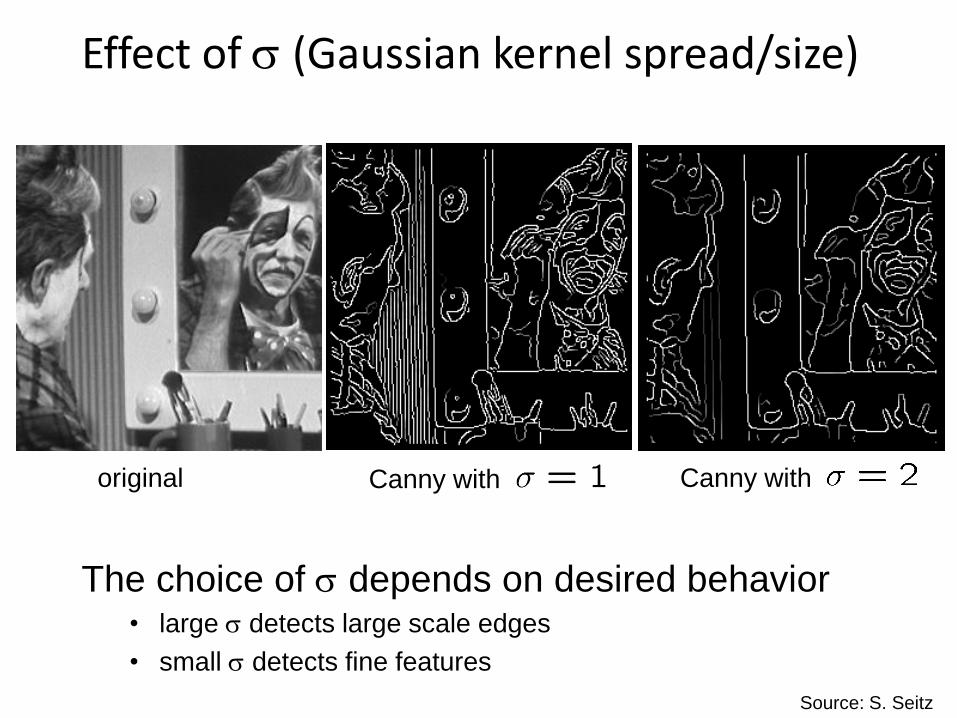
Effect of (Gaussian kernel spread/size)

Canny with Canny with original

The choice of depends on desired behavior• large detects large scale edges

• small detects fine features

Source: S. Seitz