- 1

8 ORNL/CP-97328

The BR Eigenvalue Algorithm*

G. A. Geist Computer Science and Mathematics Division

Oak Ridge National Laboratory P.O. Box 2008, Bldg. 6012 Oak Ridge, TN 3783 1-6367

G. W. Howell Department of Applied Mathematics

Florida Institute of Technology 150 W. University Blvd. Melbourne, FL 32901

, I l . in+?

LA rw% r I F+ . '1: - 5 C - ' ' D. S. Watkins Department of Pure and Applied Mathematics

Pullman, WA 99 164-3 1 13

Washington State University Y (

b OlSTRltKITloN OF THIS DOCUMENT IS WLMlTED

"This submitttd r8ianuscript i-as bcen authored by a con!ractor of the US. Govemrnevt under Contract No. nE-AC05-960R22464. Axordirgly, the US. Govern- ment retains a nonexclusive, royakyfree license to publish or reproduce the pub!ishod form of this contribution, or allow others to do so, for U.S. Govemmsnt purposes.'

*Research supported by the Applied Mathematical Sciences Research Program, Office of Energy Research, U.S. Department of Energy, under contract No. DE-AC05-960R22464 with Lockheed Martin Energy Research Corporation.

DISCLAIMER

This report was prepared as an account of work sponsored by an agency of the United States Government. Neither the United States Government nor any agency thereof, nor any of their employees, makes any warranty, express or implied. or assumes any legal liability or responsibility for the accuracy, completeness, or use- fulness of any information, apparatus, product, or process disclosed, or represents that its use would not infringe privately owned righu. Reference herein to any spe- cific commercial product, process, or sewia by trade name, trademark, manufac- turer, or otherwise does not necessarily constitute or imply its endorsement, recom- mendation, or favoring by the United States Government or any agency thereof. The views and opinions of authors expressed herein do not necessarily state or reflect those of the United States Government or any agency thereof.

c

THE BR EIGENVALUE ALGORITHM I

G. A. GEIST *, G. W. HOWELL t , AND D. S. \VATICINS

Abstract. T h e B R algorithm, a new method for calculating the eigenvalues of an upper Hes- senberg matrix, is introduced. I t is a bulge-chasingalgorithm like the Q R algorithm, but , unlike the QR algorithm, it is well adapted to computing the eigenvaluesof the narrow-band, nearly tridiagonal matrices generated by the look-ahead Lanczos process. This paper describes the B R algorithm and gives numerical evidence tha t it works well in conjunction with the Lanczos process. On the biggest problems run so far, the BR algorithm beats the QR algorithm by a factor of 30-60 in computing time and a factor of over 100 in matrix storage space.

Key words. eigenvalue computation, Q R algorithm, unsymmetric Lanczos process

AMS subject classifications. 65F15, 15A18

1. Introduction. One of the most economical tools for probing the spectrum of a large, sparse, nonsymmetric matrix is the look-ahead Lanczos algorithm [4], [7], [8]. A subproblem that arises at least twice and perhaps repeatedly in a look-ahead Lanczos run is that of calculating the eigenvalues of a nearly tridiagonal auxiliary matrix that is generated by the algorithm. After m Lanczos steps, the auxiliary matrix is m x m. If m is small, one can calculate the eigenvalues cheaply by the standard method, the QR algorithm. However, as m grows large, this step can become a bottleneck, since the cost of applying the QR algorithm grows approximately as m3. The QR algorithm does not make use of all of the structure of the auxiliary matrix; it exploits and preserves the upper Hessenberg form, but it neither exploits nor preserves the many zeros above the main diagonal. It is therefore natural to look for an algorithm that does a better job of preserving the structure.

In this paper we introduce the BR algorithm, which attempts to exploit and preserve all of the structure of the auxiliary matrix. It turns out that with rare exceptions (in our experience) it does succeed in preserving enough of the structure to run signficantly faster than the Q R algorithm. Since it stores the matrix in a banded data structure, it also requires significantly less storage space than the Q R algorithm. In our best runs we have been able to cut computer time by a factor of 60 and matrix storage space by a factor of more than 100.

The BR algorithm is a member of the family of GR algorithms [18], [16]. It is an implicit GR algorithm, which makes it a bulge-chasing algorithm [17]. Bulge-chasing algorithms operate on matrices that have been reduced t.0 upper Hessenberg form (or some comparable form). Each iteration consists of an initial transformation that disturbs the upper Hessenberg form, followed by a sequence of transformations that restore the upper Hessenberg form. Thus algorithms that transform a matrix to upper Hessenberg form lie a t the center of this subject.

In this paper we restrict our attention to real matrices. Similar algorithms can be developed for complex matrices.

'Mathematical Sciences Section, Oak Ridge National Laboratory, Box 2008, Bldg 6012, Oak Ridge, T N 37831-6367. e-mail: gstOornl.gov

t Department of Applied Mathematics, Florida Institute of Technology, 150 W. University Blvd., Melbourne, FL 32901. e-mail: howellOzach.fit.edu

$Department of Pure and Applied Mathematics, Washington State University, Pullman, Wash- ington 99164-31 13. e-mail: watkinsOwsu.edu. Mailing address: 6835 24th Avenue NE, Seattle, WA 98115-7037. Supported by the National Science Foundation under grant DMS-9403569. This manuscript was submitted for publication in February, 1997.

1

2 G. A. GEIST. G. W. HOWELL, AND D. S. WATKINS

2. Algorithms that transform a matrix to upper Hessenberg form. It is well known [19], [6], [15] that every m x m matrix can be transformed to upper Hessenberg form by an orthogonal similarity transformation in O( m3) operations. Upper Hessenberg means that ai j = 0 if i > j + 1. The transformation is effected in m-2 major steps as follows: In the first step a reflector (Householder transformation) acting on rows 2 through m transforms entries (3 , l) , . . . , (m, 1) to zero. When the transformation is applied on the right (i.e. to columns 2 through m), the first column is untouched, so the zeros are preserved. In the second step a reflector acting on rows 3 through m create zeros in entries (4 , 2 ) , . . . , (m, 2) , and so on. In general the kth step produces the desired zeros in the kth column. A venerable implementationof this procedure is the code ORTHES from EISPACK [l]. A more modern implementation, which applies the reflectors in blocks, is the code DGEHRD from LAPACK [3].

If one does not insist upon orthogonal transformations, one can use other means to create the zeros. For example, the EISPACK algorithm ELMHES [l] uses Gaussian elimination transformations with pivoting. Thus, on the first step, the largest (in magnitude) entry in positions (2 , l ) , . . . , (m, 1) is identified. if it is not already in position (2, l)] it is moved there by a row interchange. (The similarity transformation is completed by performing the corresponding column interchange.) Then appropriate multiples of the second row are subtracted from rows 3 through m to create zeros in positions (3, l), . . . , (m, 1). Multiples of columns 3 through m are added to column 2 to complete the similarity transformation.

If one uses Gaussian elimination transformations, one can often create additional zeros above the main diagonal. In fact it has long been known [19] that almost any matrix can be transformed to tridiagonal form. The first step of such a transformation can be accomplished as follows. Once the zeros have been created in the first column, if the entry in the ( 1 , 2 ) position is nonzero, it can be used as a pivot for column operations that create zeros in the first row. That is, the appropriate multiples of the second column are subtracted from columns 3 through m to produce zeros in positions ( 1 , 3 ) , . . . , (11 m). The similarity tranformation is completed by adding multiples of rows 3 through m to row 2. The important point is that these operations do not disturb the previously created zeros in column 1. However, we do not have the luxury of pivoting. A single row and column interchange at the beginning of each step determines the pivots for both the row elimination and the column elimination. Furthermore, if the (1 ,2 ) pivot entry happens to be zero, the row elimination will not be possible. More importantly, if the ( 1 , 2 ) entry is very close to zero, the eliminations will require extremely large multipliers, and the transformation will be unstable.

There have been numerous attempts to stabilize the reduction to tridiagonal form, none of which was entirely successful. Recently Howell, Geist, and Diaa [lo], [ll] developed a compromise strategy that reduces the matrix to upper Hessenberg form and also introduces as many zeros above the diagonal as possible. The resulting matrix is somewhere between tridiagonal and full upper Hessenberg. Since it .is typically a banded upper Hessenberg matrix, the algorithm is called BHESS.

The BHESS strategy is roughly as follows. For details see [lo], [ll]. On the kth step BHESS does acolumn elimination to make zeros in positions ( k + 2 , k ) , . . . , (m, k ) . It also attempts to create zeros in the kth row or some previous row that was not eliminated on an earlier step. Thus it will attempt to create zeros in positions (j, k + 2) , . . . , ( j , m), where j designates a row such that j 5 k and the ( j , k + 2 ) , . . . , ( j , m) entries are not all zero already. The row elimination will be carried out if the mul- tipliers that would be used for the column and row eliminations are not too big on

T H E BR EIGENVALUE ALGORITHM 3

average. The precise meaning of “too big” depends on a user-specified error tolerance T . If more than one row qualifies for elimination, the qualifier with the smallest j is eliminated. A row and column interchange that minimizes the maximum multiplier for row and column eliminations together is performed. This is a compromise. Once the row and column to be eliminated have been determined, the product of row and column pivots is invariant. Thus pivoting to maximize the column pivot will have the effect of minimizing the row pivot and vice versa. Rather than optimizing one or the other, BHESS chooses pivots that do as well as possible for rows and columns together.

If no row qualifies for elimination, only the column elimination is done. The maximal pivot is chosen.

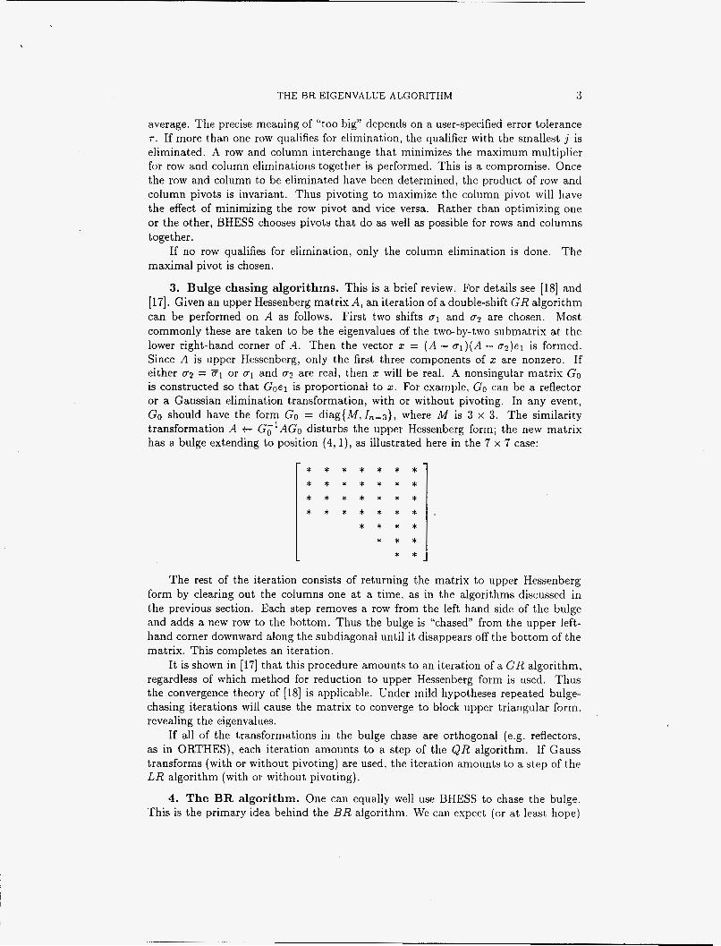
3. Bulge chasing algorithms. This is a brief review. For details see [18] and [17]. Given an upper Hessenberg matrix A , an iteration of a double-shift GR algorithm can be performed on A as follows. First two shifts u1 and uz are chosen. Most commonly these are taken to he the eigenvalues of the two-by-two submatrix at the lower right-hand corner of -4. Then the vector E = (A - a l ) ( A - u2)e l is formed. Since A is upper Hessenberg, only the first three components of x are nonzero. If either 6 2 = or 01 and ua are real, then 2 will be real. A nonsingular matrix Go is constructed so that Goel is proportional to x. For example, Go can be a reflector or a Gaussian elimination transformation, with or without pivoting. In any event, Go should have the form Go = diag{M,In-3}, where M is 3 x 3. The similarity transformation A t Gi’AGo disturbs the upper Hessenberg form; the new matrix has a bulge extending to position (4, l), as illustrated here in the 7 x 7 case:

* * * * * * * * * * * * * * * * * * * * * * * * * * * *

* * * * * * *

* * The rest of the iteration consists of returning the matrix to upper Hessenberg

form by clearing out the columns one at a time, as in the algorithms discussed in the previous section. Each step removes a row from the left hand side of the bulge and adds a new row to the bottom. Thus the bulge is “chased” from the upper left- hand corner downward along the subdiagonal until it disappears off the bottom of t,he matrix. This completes an iteration.

It is shown in [17] that this procedure amounts to an iteration of a G R algorithm. regardless of which method for reduction to upper Hessenberg form is used. Thus the convergence theory of [18] is applicable. Under mild hypotheses repeated bulge- chasing iterations will cause the matrix to converge to block upper triangular form, revealing the eigenvalues.

If all of the transformations in the bulge chase are orthogonal (e.g. reflectors, as in ORTHES), each iteration amounts to a step of the QR algorithm. If Gauss transforms (with or without pivoting) are used, the iteration amounts to a step of the LR algorithm (with or without pivoting).

4. The BR algorithm. One can equally well use BHESS to chase the bulge. This is the primary idea behind the BR algorithm. We can expect (or a t least hope)

4 G. A. GEIST, G. W. HOWELL, AND D. S. WATKINS

that iterative use of BHESS will successively narrow the band width of the matrix as it makes progress toward finding the eigenvalues. If the matrix has a narrow band width to begin with, as is the case in the look-ahead Lanczos process, repeated application of BHESS can be expected to keep it narrow.

It has to be noted, however, that when BHESS is used to chase the bulge in a narrow-band matrix, there are two mutually antagonistic forces at work. We have already seen that the algorithm is constantly trying to create new zeros above the main diagonal. This tends to reduce the band width. On the other hand, the algorithm does a certain amount of pivoting for stability. These row and column interchanges tend t o widen the band, It is not clear a priori which of these forces will prevail in the long run.

Our first experiments were disappointing. We used BHESS to perform an initial reduction to narrow-band Hessenberg form. We then applied BHESS as a bulge- chasing algorithm on the narrow-band matrix. It turned out that over the course of many iterations the band width tended to grow until the matrix became full upper Hessenberg. On inspecting the intermediate matrices we found that some extremely large numbers were building up in the part of the matrix above the main diagonal. These made row eliminations difficult. A mechanism for preventing this growth was needed.

After some experimentation we found that if a balancing operation is performed before each iteration, the undesired element growth is prevented. Our balancing operation is described as follows. For i = 1 , 2 , . . . , n multiply the i th row of the matrix by d r l and the ith column by d;, where di is chosen so that the ith row and column will have equal 1-norm after rescaling. The operations are performed in serial. That is, the scaling factor d, is determined after the first i - 1 rows and columns have been rescaled by d l , . . . , di-1. The entire scaling operation amounts to a similarity transformation A t D-'AD, where D = diag(d1,. . . , dn} .

An important difference between our scaling operation and the classical balancing routine [l], [3] is that our routine makes only one sweep through the matrix, whereas the classical routine iterates until each row's norm is nearly equal to that of the corresponding column. Our routine makes no such guarantee; the equality between row and column norms that is established for the first rows and columns will be upset by the rescaling of the later rows and columns. Nevertheless, we have found that this single sweep does a good job of shifting excess weight from the upper part of the matrix to the lower part.

The inclusion of balancing improved performance dramatically. A more refined strategy, which we use in our current code, is to balance only a small portion of the matrix a t a time. Thus we balance the first few rows (20 or so), then run the bulge through that part of the matrix, then we balance some more and run the bulge further, and so on.

Further improvements can be made by refining the elimination strategy. BHESS was developed for reducing a full matrix to a sparse form. The strategy it uses does not consider that the matrix may already have contained many zeros to begin with. Thus when BHESS is applied to a narrow-band matrix, an elimination in row i may cause the destruction of many previously existing zeros in other rows. For example, suppose that a t step i the entry in position (m, i+ 1) is used as a pivot to create zeros in positions (m , i + 2) , . . . (m, i + b ) . Then multiples of column i + 1 are subtracted from columns i + 2 , . . . , i + b. These operations can result in destruction of zeros in any other row p for which the ( p , i + 1) entry is nonzero. More importantly, multiples

T H E BR EIGENVALUE ALGORITHM .5

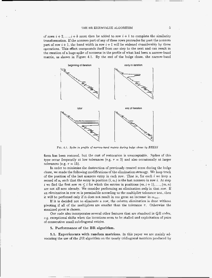
of rows i + 2 , . . . , i + b must then be added to row i + 1 to complete the similarity transformation. If the nonzero part of any of these rows protrudes far past the nonzero part of row i + 1, the band width in row i + 1 will be widened considerably by these operations. This effect compounds itself from one step to the next and can result in the creation of a huge spike of nonzeros in the profile of what had been a narrow-band matrix, as shown in Figure 4.1. By the end of the bulge chase, the narrow-band

beginning of iteration early in iteration

later end of iteration

FIG. 4.1. Spike in profile of narrow-band matrix during bulge chase by BHESS

form has been restored, but the cost of restoration is unacceptable. Spikes of this type occur frequently a t low tolerances ( e g . T = 3) and also occasionally at larger tolerances (e.g. 7 = 15).

In order to minimize the destruction of previously created zeros during the bulge chase, we made the following modifications of the elimination strategy. We keep track of the position of the last nonzero entry in each row. That is, for each i we keep a record of ai such that the entry in position (i, ai) is the last nonzero in row i. At step i we find the first row m 5 i for which the entries in positions (m, i + l ) , . . . , (rn? n ) are not all zero already. We consider performing an elimination only in that row. If an elimination in row m is permissible according to the multiplier tolerance test, then it will be perfomed only if it does not result in too great an increase in ai+l.

If it is decided not to eliminate a row, the column elimination is done without pivoting if all of the multipliers are smaller than the tolerance T . Otherwise the maximal pivot is chosen.

Our code also incorporates several other features that are standard in QR codes, e.g. exceptional shifts when the iterations seem to be stalled and exploitation of pairs of consecutive small subdiagonal entries.

5. Performance of the BR algorithm.

5.1. Experiments with random matrices. In this paper we are mainly ad- vocating the use of the B R algorithm on the nearly tridiagonal matrices produced by

6 G . A. GEIST. G . \V. HOWELL, AND D. S . WATKINS

the look-ahead Lanczos process. Nevertheless, we shall begin by reporting on some ex- periments with full matrices. The numbers reported in this subsection were obtained using an early version of the algorithm that does a complete rebalance between bulge chases and no rebalancing during a bulge chase.

We constructed random matrices with known eigenvalues by the following proce- dure. First a random block upper triangular matrix T + N is constructed. T is the block diagonal part. It has 1 x 1 and 2 x 2 blocks; its eigenvalues are obvious, and these are the eigenvalues of the matrix. The eigenvalues and the entries of N are normally distributed with mean zero and standard deviations UT and U N , respectively. The ratio CTT/UN is adjusted to control the ratio S = 1 1 NIIF/IITIIF, which is a measure of departure from normality. We also control the number of complex eigenvalues. We then produce a matrix A with the same eigenvalues by applying a random orthogonal similarity transformation (uniform with respect to Haar measure on the orthogonal group) by the method of Stewart [14].

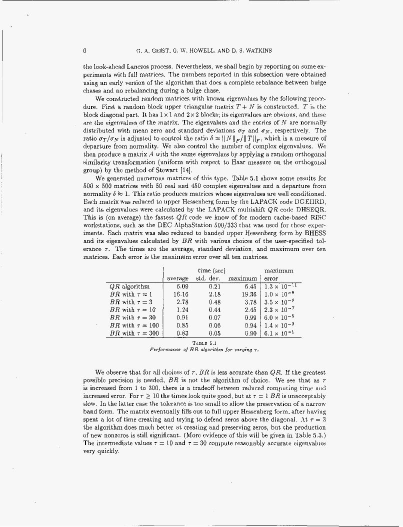
We generated numerous matrices of this type. Table 5.1 shows some results for 500 x 500 matrices with 50 real and 450 complex eigenvalues and a departure from normality 6 k 1. This ratio produces matrices whose eigenvalues are well conditioned. Each matrix was reduced to upper Hessenberg form by the LAPACK code DGEHRD, and its eigenvalues were calculated by the LAP.L\CI< multishift QR code DHSEQR. This is (on average) the fastest QR code we know of for modern cache-based RISC workstations, such as the DEC Alphastation 500/333 that was used for these esper- iments. Each matrix was also reduced to banded upper Hessenberg form by BHESS and its eigenvalues calculated by BR with various choices of the user-specified tol- erance r. The times are the average, standard deviation, and maximum over ten matrices. Each error is the maximum error over all ten matrices.

QR algorithm BR with T = 1 BR with r = 3 BR with T = 10 BR with T = 30 BR with T = 100 BR with T = 300

time (sec) average std. dev. maximum

6.09 0.21 6.45 16.16 2.18 19.36 2.78 0.48 3.78 1.24 0.44 2.45 0.91 0.07 0.99 0.85 0.06 0.94 0.83 0.05 0.90

maximurn error 1.3 x lo-"

3.5 x 2.3 x

1.0 x 10-9

6.0 x 10-5 1.4 x 10-3 6.1 x lo-'

TABLE 5.1 Performance of BR algorithm for varying T.

We observe that for all choices of r , BR is less accurate than QR. If the greatest possible precision is needed, BR is not the algorithm of choice. We see that as r is increased from 1 to 300, there is a tradeoff between reduced computing time and increased error. For r 2 10 the times look quite good, but at T = 1 BR is unacceptably slow. In the latter case the tolerance is too small to allow the preservation of a narrow band form. The matrix eventually fills out to full upper Hessenberg form, after having spent a lot of time creating and trying to defend zeros above the diagonal. At T = 3 the algorithm does much better a t creating and preserving zeros, but the production of new nonzeros is still significant. (More evidence of this will be given in Table 5.3.) The intermediate values T = 10 and T = 30 compute reasonably accurate eigenvalues very quickly.

T H E BR EIGENVALUE ALGORITHM

Departure from normality

0.0

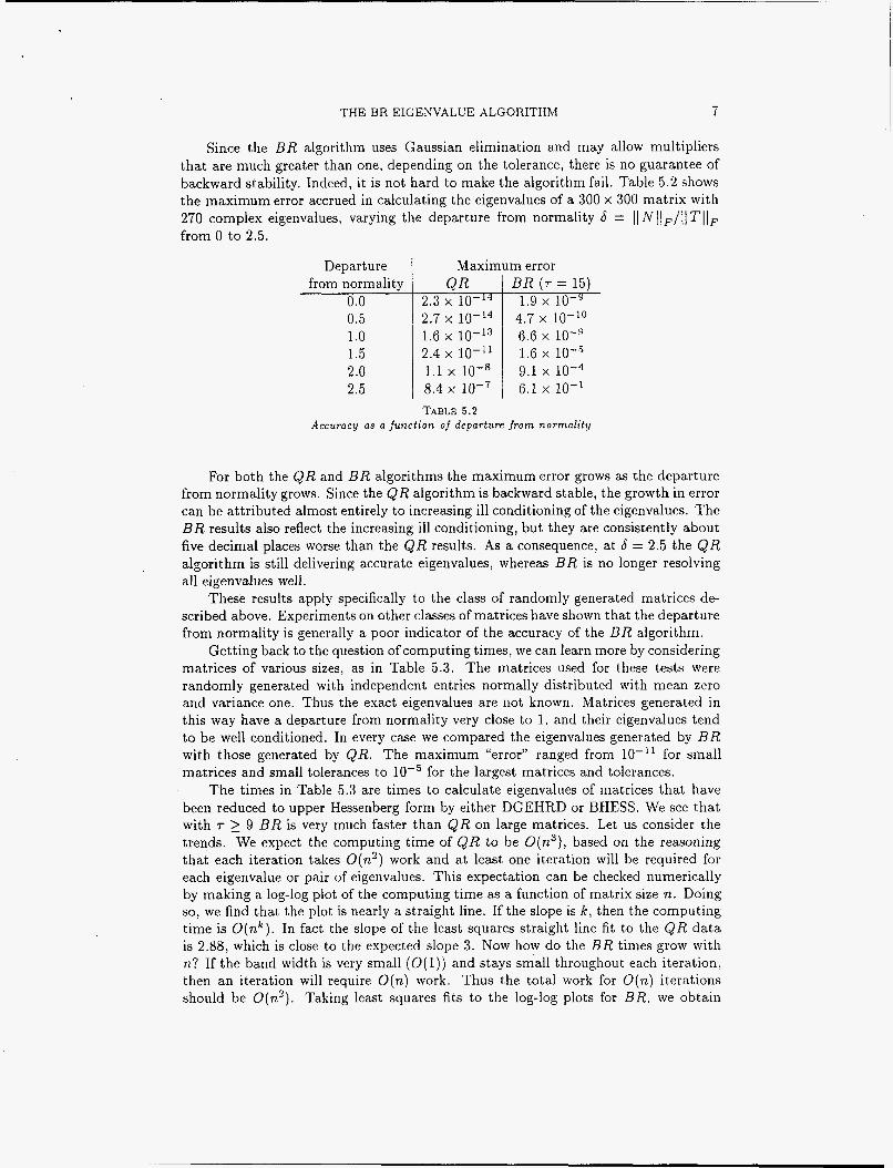
Since the BR algorithm uses Gaussian elimination and may allow multipliers that are much greater than one, depending on the tolerance, there is no guarantee of backward stability. Indeed, it is not hard to make the algorithm fail. Table 5.2 shows the maximum error accrued in calculating the eigenvalues of a 300 x 300 matrix with 270 complex eigenvalues, varying the departure from normality 6 = 1 1 NIIF/IITIIF from 0 to 2.5.

Maximum error Q R BR (T = 15)

2.3 x 1.9 x

1.6 x 6.6 x lo-' 2.4 x lo-'' 1.6 x 1.1 x 9.1 x 8.4 x 6.1 x lo-'

2.7 x 10-14 4.7 x 10-10 0.5 1 .o 1.5 2.0 2.5

TABLE 5.2 Accuracy as a function of departure f rom normality

For both the QR and B R algorithms the maximum error grows as the departure from normality grows. Since the QR algorithm is backward stable, the growth in error can be attributed almost entirely to increasing ill conditioning of the eigenvalues. The B R results also reflect the increasing ill conditioning, but they are consistently about five decimal places worse than the QR results. As a consequence, at 6 = 2.5 the QR algorithm is still delivering accurate eigenvalues, whereas B R is no longer resolving all eigenvalues well.

These results apply specifically to the class of randomly generated matrices de- scribed above. Experiments on other classes of matrices have shown that the departure from normality is generally a poor indicator of the accuracy of the B R algorithm.

Getting back to the question of computing times, we can learn more by considering matrices of various sizes, as in Table 5.3. The matrices used for these tests were randomly generated with independent entries normally distributed with mean zero and variance one. Thus the exact eigenvalues are not known. Matrices generated in this way have a departure from normality very close to 1, and their eigenvalues tend to be well conditioned. In every case we compared the eigenvalues generated by B R with those generated by QR. The maximum "error" ranged from lo-" for small matrices and small tolerances to lod5 for the largest matrices and tolerances.

The times in Table 5.3 are times to calculate eigenvalues of matrices that have been reduced to upper Hessenberg form by either DGEHRD or BHESS. We see that with 7 2 9 B R is very much faster than QR on large matrices. Let us consider the trends. We expect the computing time of QR to be O(n3) , based on the reasoning that each iteration takes O(n') work and at least one iteration will be required for each eigenvalue or pair of eigenvalues. This expectation can be checked numerically by making a log-log plot of the computing time as a function of matrix size n. Doing so, we find that the plot is nearly a straight line. If the slope is k, then the computing time is O ( n k ) . In fact the slope of the least squares straight line fit to the QR data is 2.88, which is close to the expected slope 3. Now how do the BR times grow with n? If the band width is very small (O(1)) and stays small throughout each iteration. then an iteration will require O ( n ) work. Thus the total work for O ( n ) iterations should be O ( n 2 ) . Taking least squares fits to the log-log plots for BR, we obtain

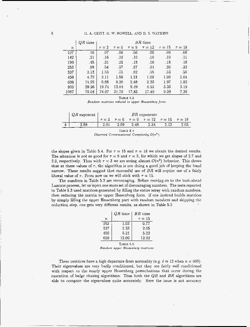
a

QR exponent

k 2.88

G. A. GEIST. G. W. HOWELL. AND D. S. L\’ATI<INS

BR exponents ~ = 3 T = G r = 9 r = 1 2 r = 1 5 ~ = 1 8

2.91 2.69 2.48 2.34 2.12 2.03

n 107 142 190 253 337 450 GOO 800

1067

QR time

.10

.21

.45

.98 2.13 4.79

11.92 29.26 79.04

B R time ~ = 3 T = G ~ = 9 r = 1 2 ~ = 1 5 ~ = 1 8

.07 .06 .06 .OG .0G .06

.16 .10 .10 .10 .10 .ll

.31 .21 .18 . l 8 . l 8 .18

.54 .37 .37 .34 .36 .33 1.53 .T5 .G2 .55 .53 .5G 3.11 1.56 1.21 1.09 1.06 1.04 G.68 6.26 2.48 2.23 1.97 1.82

19.74 13.04 9.49 4.55 3.39 3.19 74.07 21.76 17.85 17.49 9.20 7.36

TABLE 5.3 R a n d o m matrices reduced t o upper Hessenberg f o r m

TABLE 5 . 4 Observed Computational Compleri ty O ( n k )

the slopes given in Table 5.4. For T = 15 and r = 18 we obtain the desired results. The situation is not so good for T = G and r = 3, for which we get slopes of 2.7 and 2.9, respectively. Thus with T = 3 we are seeing almost O(n3) behavior. This shows that at these values of r , the algorithm is not doing a good job of keeping the band narrow. These results suggest that successful use of B R will require use of a fairly liberal value of T . From now on we will stick with T = 15.

The numbers in Table 5.3 are encouraging. Before moving on to the look-ahead Lanczos process, let us inject one more set of discouraging numbers. The tests reported in Table 5.3 used matrices generated by filling the entire array with random numbers. then reducing the matrix to upper Hessenberg form, If one instead builds matrices by simply filling the upper Hessenberg part with random numbers and skipping the reduction step, one gets very different results, as shown in Table 5.5

QR time B R time r = 15 #-2+ 0.77’

5.21 5.22 GOO 12.00 12.02

TABLE 5 . 5 R a n d o m upper Hessenberg matrrces

These matrices have a high departure from normality (e.g. 6 x 12 when n = 600). Their eigenvalues are very badly conditioned, but they are fairly well conditioned with respect to the nearly upper Hessenberg perturbations that occur during the execution of bulge chasing algorithms. Thus both the QR and B R algorithms are able to compute the eigenvalues quite accurately. Here the issue is not accuracy

THE BR EIGENVALUE ALGORITHM H

but computing time. While the QR times are not much different than they were in Table 5.3 . the BR times with i- = 15 are much worse. Indeed they are no better than the QR times. Matrices of this type have so much weight above the main diagonal that it is difficult to get them into a narrow-band form. .4s a consequence BR ends up doing as much work as QR.

5.2. Experiments with sparse matrices. We performed numerous experi- ments in which we used the BR algorithm to calculate the eigenvalues of the nearly tridiagonal matrices generated by the look-ahead Lanczos process. These are upper Hessenberg, so we can apply BR directly to them; there is no need to preprocess them by BHESS. We modified the code DULAL from the package QMRPACK by Freund and Nachtigal [5]. In that code the eigenvalue computation is clone by the QR algo- rithm in a standard array data structure. We switched to a banded storage scheme and replaced QR by BR. In many cases we ran both QR and BR for comparison purposes. DULAL uses the EISPACK code HQR, but we substituted the LAPACK code DHSEQR, which is usually faster than HQR on the DEC Alphastation 500/333 and similar machines.

Another change we made was in the balancing strategy of BR. Instead of rebal- ancing the whole matrix once before each bulge chase, we rebalance small sections of the matrix during the bulge chase, as described earlier. That is, we balance the first few rows, then run the bulge through that part of the matrix, then we balance some more and run the bulge further, and so on. This change reduces the growth of the bandwidth significantly. This is an important improvement, since the matrix now has to be kept within the confines of a banded data structure.

In the experiments reported below, the matrices produced by the look-ahead Lanczos process were always very nearly tridiagonal. If the look-ahead feature is not used a t all, a tridiagonal matrix is formed. Each time the look-ahead is used, a small bulge on the upper side of the band is formed. In our experiments no more than four look-aheads were needed in any given run. The upper bandwidths of the resulting matrices never exceeded 3. A more typical upper bandwidth was 2, and in many cases it was 1 (tridiagonal), indicating that no look-ahead steps had been needed.

Convection-diffusion matrices. Our first examples are matrices obtained by discretizing a three-dimensional convection-diffusion operator

on the domain $2 = (0, 1)3 with u = 0 on 8Q. The standard second-order centered finite-difference approximations were used.

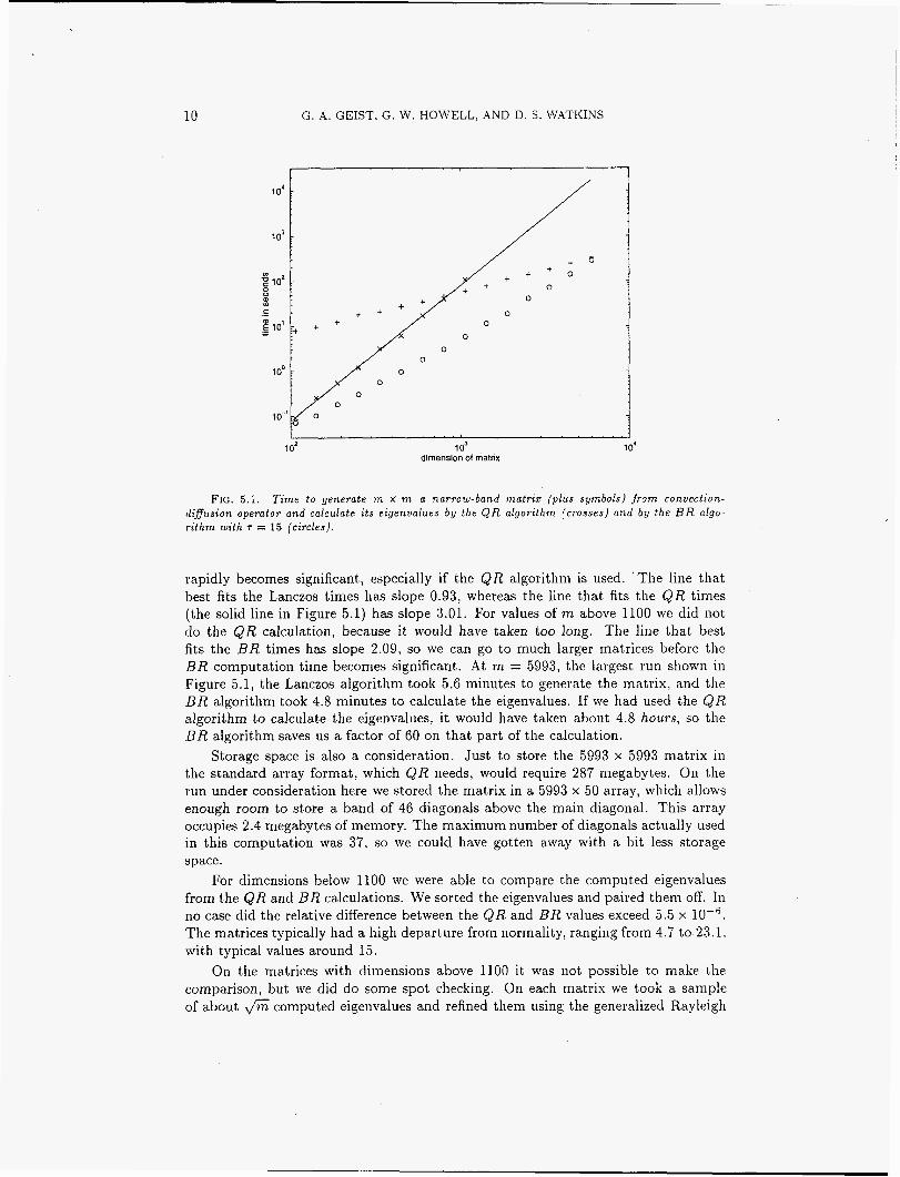
With a mesh size h = & in each direction, we obtain a matrix of order 3g3 = 59319. Each row has seven nonzero entries. We chose the convection coefficient c = 8 to get a PCclet number 9 = 0.1. We ran rn look-ahead Lanczos steps and calculated the eigenvalues of the m x rn narrow-band matrix for various choices of m ranging from about 100 to 6000. In Figure 5.1 we display the time to generate the matrix (plus symbols), the time to calculate its eigenvalues by the QR algorithm (cross symbols), and the time to calculate the eigenvalues by the BR algorithm (circle symbols) with T = 15.

We see that BR is cheaper than QR for all m in the range that we studied, but for small matrices it does not matter which method we use. Both algorithms can calculate the eigenvalues in a small fraction of the time it takes to generate the matrix. As the matrix dimension increases, the time spent computing eigenvalues

10

io4

10’ I

< l o 2 i + +

._ E 10’ :+

8 i $ : 0 c . .- 0

c :

too : i

i J

G. A. GEIST, G. W. HOWELL, AND D. S. \.VATICINS

+ + + / o 0

FIG. 5.1. T i m e to generate m x m a narrow-band mat r i x (plus symbols) f r o m convection- di f fusion operator and calculate i ts eigenvalues by the QR algorithm (crosses) a n d by the B R algo- r i t hm with r = 15 (circles).

rapidly becomes significant, especially if the QR algorithm is used. ‘ T h e line that best fits the Lanczos times has slope 0.93, whereas the line that fits the QR times (the solid line in Figure 5.1) has slope 3.01. For values of rn above 1100 we did not do the QR calculation, because it would have taken too long. The line that best fits the B R times has slope ’2.09, so we can go to much larger matrices before the B R computation time becomes significant. At m = 5993, the largest run shown in Figure 5.1, the Lanczos algorithm took 5.6 minutes to generate the matrix, and the B R algorithm took 4.8 minutes to calculate the eigenvalues. If we had used the QR algorithm to calculate the eigenvalues, i t would have taken about 4.8 hours, so the B R algorithm saves us a factor of 60 on that part of the calculation.

Storage space is also a consideration. Just to store the 5993 x 5993 matrix in the standard array format, which QR needs, would require 287 megabytes. On the run under consideration here we stored the matrix in a 5993 x 50 array, which allows enough room to store a band of 46 diagonals above the main diagonal. This array occupies 2.4 megabytes of memory. The maximum number of diagonals actually used in this computation was 37, so we could have gotten away with a bit less storage space.

For dimensions below 1100 we were able to compare the computed eigenvalues from the QR and B R calculations. We sorted the eigenvalues and paired them off. In no case did the relative difference between the QR and B R values exceed 5.5 x The matrices typically had a high departure from normality, ranging from 4.7 to 23.1. with typical values around 15.

On the matrices with dimensions above 1100 it was not possible to make the comparison, but we did do some spot checking. On each matrix we t-ook a sample of about fi computed eigenvalues and refined them using the generalized Rayleigh

THE BR EIGENVALUE .4LGORITHM 11

B R time T = 15

0.95 0.90 1.07 *** *** *** 0.85 0.85

quotient iteration code GIRI [13]. In no case did the relative difference between the original computed value and the refined value exceed 1.2 x

We have focused on how well B R calculates the eigenvalues of the m x m narrow- band matrix. Typically only a few of these will be good approximations to the eigen- values of the large sparse matrix. The question of which ones are “good” is difficult and obviously important. We are ignoring it here, because our objective is simply to study how well the BR algorithm does its assigned task.

Harder PQclet numbers. One can make the B R algorithm fail on convection- diffusion problems by making the PCclet number closer to 1. When it is exactly 1, all of the eigenvalues of the convection diffusion operator coalesce into a single highly defective eigenvalue. The Jordan canonical form consists of one gigantic Jordan block. and the eigenvalue is catastrophically ill conditioned. For Pkclet numbers near 1 the eigenvalues are distinct but crowded. and they are all ill conditioned.

Table 5.6 lists the outcomes of runs with a variety of PCclet numbers. In these experiments a coarser grid with h = 1/20 was used. The dimension of the convection- diffusion matrix was thus 1g3 = 6859. The look-ahead Lanczos process was run for 450 steps (taking about 2.5 seconds), and the eigenvalues of the resulting 450 x 450 matrix were calculated by by both the QR and B R algorithms.

Max. rel. “error”

2.4 x 5.2 x lo-’ 7.2 x ***

*** ***

4.2 x 1.3 x lo-’

Pkclet number

0.1 0.2 0.4 0.6 1.5 2.0 3.0 6.0

QR time

5.38 6.54 (3.46 4.39 5.35 5.55 4.78 5.02

Max. upper bandwidth [ B R )

8 12 14 ** ** ** T T

convection-diffusion operators with various Pe‘clet numbers

For PCclet numbers far from 1, the B R algorithm returns good results in about one sixth the time as QR. For three values nearer 1. B R returned without calculating the eigenvalues, because it needed more space than was allocated. That is, the band width blew up. We had allocated enough room for a band of 42 diagonals above the main diagonal. The numbers in the last column of Table 5.6 show that this was far more than enough room for those runs that were successful. For the unsuccessful runs, 42 diagonals was far less than enough. On a subsequent attempt we increased the maximum bandwidth to 120, but that still was not enough. By taking the band width large enough, we would eventually be able to make the code work. However, our experiences with the earlier version of the code suggest that bandwidth blowups are a sign of trouble that should not be ignored. They cause a severe increase in computing time, and the computed eigenvalues are likely to be inaccurate. We suggest that B R be used with a modest maximum bandwidth. If it cannot solve the problem within the allocated space, it probably will not be able to solve the problem economically or accurately.

Another way to deal with bandwidth blowups is to increase the tolerance T . When we set 7- a t 100. BR succeeded for all three of the PCclet numbers for which it had

12 G. A. GEIST, G . W. HOWELL, AND D. S. WATKINS

10'

io3

failed at i- = 15. It also succeeded for P6clet numbers 0.9 and 1.1. Execution times were under one second. However, the results agreed with those computed by QR to only about one decimal place. This is partly due to loss of accuracy caused by taking such a high tolerance. However, the values computed by QR should not necessarily be accepted as correct, since most of the eigenvalues are extremely ill conditioned.

r

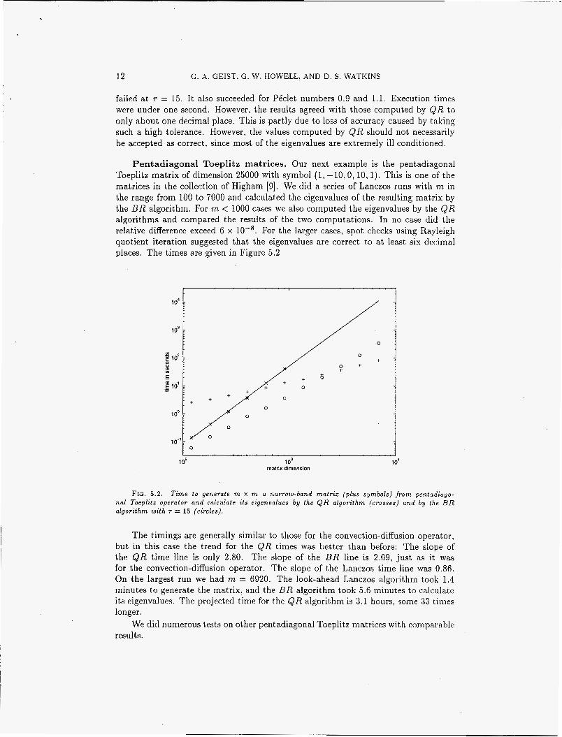
Pentadiagonal Toeplitz matrices. Our next example is the pentadiagonal Toeplitz matrix of dimension 25000 with symbol (1,-'10,0, 10, 1). This is one of the matrices in the collection of Higham [9]. We did a series of Lanczos runs with m in the range from 100 to 7000 and calculated the eigenvalues of the resulting matrix by the B R algorithm. For m < 1000 cases we also computed the eigenvalues by the QR algorithms and compared the results of the two computations. In no case did the relative difference exceed G x For the larger cases, spot checks using Rayleigh quotient iteration suggested that the eigenvalues are correct t,o at least six decimal places. The times are given in Figure 5.2

/ o o + e +

f 1 o2 1 o3

matrix dimension 1 o4

FIG. 5.2 . T i m e to generate m x m a narrow-band matr ix (p lus symbols) f r o m pentadiago- nal Toeplitz operator and calculate i ts eigenvalues by the QR algorithm (crosses) and b y the B R algorithm wi th T = 15 (circles).

The timings are generally similar to those for the convection-diffusion operator, but in this case the trend for the QR times was better than before: The slope of the QR time line is only 2.80. The slope of the BR line is 2.09, just as it was for the convection-diffusion operator. The slope of the Lanczos time line was 0.86. On the largest run we had m = 6920. The look-ahead Lanczos algorithm took 1.4 minutes to generate the matrix, and the BR algorithm took 5.6 minutes to calculate its eigenvalues. The projected time for the QR algorithm is 3.1 hours, some 33 times longer.

We did numerous tests on other pentadiagonal Toeplitz matrices with comparable results.

T H E BR EIGENVALUE ALGORITHM 1 :3

Tolosa matrix. We performed the same sequence of experiments on a Tolosa matrix of dimension 40,000. which we obtained from the collection of Bai et. al. [ a ] . The results were nearly identical to those shown in Figure 5.2, except that we were unable to get B R (with tolerance r = 15) to run for matrices above about 3000, because the bandwidth would not stay within the constraint that we had imposed (46 bands above the main diagonal). We remedied this by increasing r to 30. We were then able to run rn up to 7000 with modest band widths.

Other matrices. We also experimented with several other matrices from the collection of Bai et. al. [a ] , including the Brusselator wave model of a chemical re- action, the Ising model for ferromagnetic materials, and the Navier-Stokes matrix of dimension 23560 from Mahajan, Dowell, and Bliss [12]. In all cases the BR algo- rithm was able to calculate the eigenvalues of the narrow-band matrices produced by look-ahead Lanczos quickly and with reasonable accuracy.

Upper Hessenberg Examples. A few of the standard test matrices are narrow- band upper Hessenberg matrices to begin with. We can apply the BR algorithm directly to these matrices, without having to preprocess them by BHESS or look- ahead Lanczos.

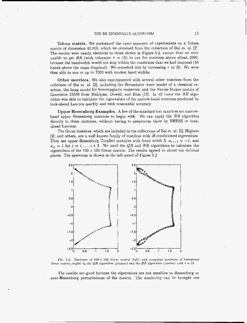
The Grcar matrices, which are included in the collections of Bai et. al. [2], Higham [9], and others, are a well known family of matrices with ill-conditioned eigenvalues. They are upper Hessenberg Toeplitz matrices with band width 5, ai , i - l = -1, and aij = 1 for j = i, . . . , i + 3. We used the QR and B R algorithms to calculate the eigenvalues of the 100 x 100 Grcar matrix. The results agreed to about ten decimal places. The spectrum is shown in the left panel of Figure 5.3

-2.5' I 0 0.5 1 1.5 2

-2.5' 0 0.5 1 1.5

F I G . 5 .3 . Spectrum of 100 x 100 Grcar matrix (left) , and computed spectrum of transposed Grcar matrix (right) by the Q R algorithm ( p l u s e s ) and the B R algorithm (circles) with T = 15

The results are good because the eigenvalues are not sensitive to Hessenberg or near-Hessenberg perturbations of the matrix. The sensitivity can be brought out

14 G. A. GEIST, G . W. HOWELL, AND D. S . WATKINS

by transposing the matrix. We used the LAPACK code DGEHRD to reduce the transposed matrix to upper Hessenberg form, then we applied the QR algorithm. The resulting computed spectrum is given by plus symbols in the right panel of Figure 5.3. We also used BHESS to reduce the transposed matris to banded upper Hessenberg form, and then applied the B R algorithm. The results are given by circle svinbols in the figure. We observe that both QR and BR failed to resolve the eigenvalues a t the ends of the spectrum accurately, and both failed by about the same amount.

The Clement matrices, which are also in the collection of Higham, are n x 72

tridiagonal matrices with ai,i-1 = i - 1, aii = 0, and ai,i+l = n - i . Thus the 4 x 4 Clement matrix is

It is diagonally similar to a they are the integers X j = eigenvalues ill conditioned.

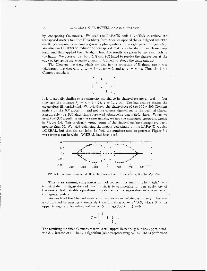
symmetric matrix, so its eigenvalues are all real; in fact n + 1 - 2 j , j = 1, . . . , T I . The bad scaling makes the We calculated the eigenvalues of the 300 x 300 Clement -

matrix by the BR algorithm and got the correct eigenvalues to ten decimal places. Presumably the BR algorithm's repeated rebalancing was helpful here. When we used the QR algorithm on the same matrix, we got the computed spectrum shown in Figure 5.4. This is clearly wrong; some of the eigenvalues have imaginary parts greater than 50. We tried balancing the matrix beforehand by the LAPACK routine DGEBAL, but that did not help. In fact, the numbers used to generate Figure 5.4 were from a run in which DGEBAL had been used.

-300 -200 -100 0 100 200 300

+ + ++++++

+ +++

+ + +++++++++

F I G . 5 . 4 . Incorrect spectrum of 300 x 300 Clement matrix computed b y the Q R algorithm.

This is an amusing comparison but, of course, it is unfair. The "right" way to calculate the eigenvalues of this matrix is to symmetrize it, then apply any of the several fast, reliable algorithms for calculating the eigenvalues of a symmetric, tridiagonal matrix.

We modified the Clement matrix to disguise its underlying symmetry. This was accomplished by making a similarity transformation A + S-'AS, where S is the upper triangular, block-diagonal matrix S = diag{U, U, U, . . .} with

The resulting modified Clement matrix is still upper Hessenberg but has upper band- width 2, instead of 1. The QR algorithm (with preprocessing by DGEBAL) performed

THE BR EIGENVALUE ALGORITHM 15

even worse on this matrix. In the 200 x 200 case it produced computed eigenvalues with imaginary parts as large as 50. The computed spectrum was similar in appear- ance to the spectrum shown in Figure 5.4. In contrast, the B R algorithm was able to compute the correct eigenvalues to ten decimal places.

One can build modified Clement matrices with arbitrarily thick bands by ap- plying further similarity transformations with matrices like S. We performed a few experiments along those lines with results similar to what we have reported here.

6. Concluding remarks. We have introduced the BR algorithm and shown that it does a good job of computing the eigenvalues of the narrow-band upper Hes- senberg matrices produced by the look-ahead Lanczos process. Although the B R algorithm can sometimes fail, our experience has been that failures are rare. The BR algorithm is usually much faster than the QR algorithm, and it needs much less storage space. Experiments suggest that its execution time is little more than O(m') as the matrix size rn becomes large, provided that a liberal multiplier tolerance (e.g. T = 15) is used. Since large multipliers are allowed, we cannot claim that the al- gorithm is st,able. Thus the raw output of the algorithm should not be accepted as accurate spectrum without further testing. In the context of the Lanczos process such further testing is carried out routinely, since it is also necessary to decide which of the eigenvalues of the narrow-band matrix are indeed good approximations to eigenvalues of the original large matrix.

REFERENCES

[I] B. T. SMITH ET. AL., Matrix Eigensystem Routines-EISPACK Guide, Springer-Verlag, New York, 2 ed., 1976.

[2] Z. BAI, D. DAY, J . DEMMEL, AND J . DONGARRA, A test matrix collection for nonhermitian eigenvalue problems, tech. rep., University of Kentucky, 1996. Available by anonymous f tp from ftp.ms.uky.edu. (cd pub/misc/bai).

[3] E. ANDERSON ET. AL., LAPACK Users' Guide, SIAM, Philadelphia, 1992. [4] R. W. FREUND, M. H. GUTKNECHT, A N D N . M. NACHTIGAL, An implementation of the look-

ahead lanczos algorithm for non-hermitian matrices, SIAM J . Sci. Comput., 14 (1993),

[5] R. W. FREUND, N. M. NACHTIGAL, AND J . C . REEB, QMRP.4CA' Users' pp. 137-158.

Guide, Tech. Rep. ORNL/TM-I2807, Oak Ridge National Laboratory, 1994. . http://www.epm.ornl.gov/Nsanta/.

[6] G. H. GOLUB AND C. F. VAN LOAN, Matriz Computations. Johns Hopkins University Press, Baltimore, third ed., 1996.

[7] M . H. GUTKNECHT, A completed theory of the unsymmetric lanczos process and related a lgo - ri thms. Part I , SIAM J . Matrix Anal. Appl., 13 (1992), pp. 594-639.

PI - . d completed theory of the unsymmetric lanczos process and related algorithms, Part I I , SIAM J . Matrix Anal. Appl., 15 (1994), pp. 15-58.

[9] N. J . HIGHAM. The test matrix t o o l b o z f o r MATLAB, Tech. Rep. 276, University of Manchester, Manchester, England, 1995. http://www.ma.rnan.ac.uk/~higham/testmat.html.

[IO] G. W. HOWELL, G. A. GEIST, AND N. DIAA, Gaussian reduction t o a similar near-tridiagonal Hessenberg form: Algorithm BHESS. preprint, June 1995.

[Ill G. W. HOWELL, G. A. GEIST, A N D T. ROWAN, Error analysis of reduction t o similar banded Hessenberg form, Tech. Rep. ORNL/TM-13344. Oak Ridge National Laboratory, March 1998.

[12] A. MAHAJAN, E. H. DOWELL, A N D D. BLISS, Eigenvalue calculation procedure for n n

Euler/Nauier-Stokes solver with applications t o f lows over airfoils, J . Cump. Phys.. 97

[13] G. SCHRAUF, Algorithm 696, An inverse rayleigh iteration f o r complex band matrices. ACM

[14] G . W. STEWART, The eflcient generation of random orthogonal matrices with an application

[15] D. S. WATKINS, Fundamentals of Matriz Computations. John Wiley and Sons, New York. 1991.

(1991), pp. 398-413.

Trans. Math. Software, 17 (1991), pp. 335-340.

to condition estimators, SIAM J. Numer. Anal., 17 (1980), pp. 403-409.

1F G. A. GEIST, G . W. HOWELL, AND D. S. \VATI<INS

[16] -, QR-like algortthms--an overview of convergence theory and practice, in The Mathe- matics of Numerical Analysis. J . Renegar, M. Shub, and S. Smale, eds., vol. 32 of Lectures in Applied Mathematics, American Mathematical Society. 1996.

[17] D. s. W A T K I N S A N D L. ELSNER, Chaszng algortthms f o r the eigenvalue problem. SIAM J . Matrix Anal. Appl., 12 (1991), pp. 374-384.

[I81 - , Convergence of algorithms of decompositton type f o r the eigenvalue problem, Linear Algebra Appl., 143 (1991), pp. 19-4i.

[19] J. H. WILKINSON, T h e Algebratc Eigenvalue Problem,, Clarendon Press, Oxford University, 1965.

M98004819 I11111111 111 11111 lllll1llll111111111111111 lllll11111111

Publ. Date (1 1) 7 Sponsor Code (18) E/? g XF

DOE