Embed Size (px)
Citation preview

THE CAKRAVĀLA METHOD
FOR SOLVING
QUADRATIC INDETERMINATE EQUATIONS
M.D.SRINIVAS CENTRE FOR POLICY STUDIES

OUTLINE
• The vargaprakçti equation X2 – D Y2 = K, and Brahmagupta’s bhāvanā process (c. 628 CE).
• The cakravāla method of solution of Jayadeva (c. 10th cent) and Bhāskara (c.1150).
• Bhāskara’s examples X2 – 61Y2 = 1, X2 – 67Y2 = 1. • Analysis of the cakravāla method by Krishnaswami
Ayyangar. • History of the so called "Pell’s Equation" X2 - D Y2 = 1. • Solution of "Pell’s equation" by expansion of √D into a simple
continued fraction (c. 18th cent). • Bhāskara semi-regular continued fraction expansion of √D • Optimality of the cakravāla method.

VARGA PRAKèTI
In Chapter XVIII of his Brāhmasphuña-siddhānta (c.628 CE),
Brahmagupta considers the problem of solving for integral values of X,
Y, the equation
X2 – D Y2 = K,
given a non-square integer D > 0, and an integer K.
X is called the larger root (jyeùñha-mūla), Y is called the smaller root
(kaniùñha-mūla), D is the prakçti, K is the kùepa.
One motivation for this problem is that of finding rational approximations to square-root of D. If X, Y are integers such that X2 - D Y2 = 1, then,
The Śulva-sūtra approximation (prior to 800 BCE):
√2 ≈ 1+ 1/3 + 1/3.4 - 1/3.4.34 = 577/408 [(577)2 - 2 (408)2 = 1]

BRAHMAGUPTA’S BHĀVANĀ
मलू ंि धे वगार्द ्गणुकगणुािद यतुिवहीना । आ वधो गणुकगणुः सहान्त्यघातने कृतमन्त्यम॥् व वधकै्य ं थम ं क्षपेःक्षपेवधतलु्यः।
क्षपेशोधकहृत ेमलू े क्षपेके रूप॥े
If X12 – D Y1
2 = K1 and X22– D Y2
2 = K2 then
(X1 X2 ± D Y1Y2)2 – D (X1 Y2 ± X2Y1)2 = K1 K2
In particular given X2 -D Y2 = K, we get the rational solution
[(X2 + D Y2)/K]2 - D [(2XY)/K]2 = 1
Also, if one solution of the Equation X2- D Y2 = 1 is found, an infinite
number of solutions can be found, via
(X, Y) (X2 + D Y2, 2XY)

USE OF BHĀVANĀ WHEN K = -1, ±2, ±4
The bhāvanā principle can be use to obtain a solution of the equation
X2 – D Y2 = 1,
if we have a solution of the equation
X12 – D Y1
2 = K, for K = -1, ±2, ±4.

BRAHMAGUPTA’S EXAMPLES
रािशकलाशेषकृित ि नवितगुिणता ं यशीितगिुणता ंवा। सैकां ज्ञिदन ेवग कुवर् ावत्सरा णकः॥ To solve, X2 – D Y2 = 1, for D = 92, 83:
102 - 92.12 = 8
Doing the bhāvanā of the above with itself, 1922 - 92.202 = 64 [102 + 92.12 = 192 and 2.10.1 = 20]
Dividing both sides by 64,
242 – 92.(5/2)2 = 1
Doing the bhāvanā of the above with itself,
11512 – 92.1202 = 1 [242 + 92.(5/2)2 = 1151 and 2.24.(5/2) = 120]
Similarly,
92 - 83.12 = -2
Doing the bhāvanā of the above with itself,
1642 – 83.182 = 4 and hence, 822 – 83.92 = 1.

CAKRAVĀLA: THE CYCLIC METHOD
The first known description of the Cakravāla or the Cyclic Method occurs
in a work of Udayadivākara (c.1073), who cites the verses of Ācārya
Jayadeva.
In his Bījagaõita, Bhāskarācārya (c.1150) has given the following
description of the cakravāla method:
स्वज्ये पदक्षेपान् भाज्य क्षेपभाजकान्। कृत्वा कल्प्यो गुणस्त तथा कृितत यतुे॥ गुणवग कृत्योनेऽथवाल्पं शेषकं यथा। त ुक्षेपहृतं क्षेपो स्तः कृितत युते॥ गुणलिब्धः पद ं स्वं ततो ज्ये मतोऽसकृत्। त्यक्त्वा पूवर्पदक्षेपां वालिमद ंजगुः॥ चतु कयुताववेमिभ े भवतः पद।े चतुि क्षपेमूलाभ्यां रूपक्षेपाथर्भावना॥

THE CAKRAVĀLA METHOD
Given Xi, Yi, Ki such that Xi 2 – D Yi
2 = Ki
First find Pi+1 as follows:
(I) Use kuññaka process to solve (the linear indeterminate equation)
(Yi Pi+1 + Xi)/ |Ki| = Yi+1
for integral Pi+1, Yi+1
(II) Of the solutions of the above, choose Pi+1 >0, such that
|(Pi+12 - D)| has the least value
Then set
Ki+1 = (Pi+1 2 - D)/ Ki
Yi+1= (Yi Pi+1 + Xi)/ |Ki|
Xi+1= (Xi Pi+1 + DYi)/ |Ki|
These satisfy Xi+12 - D Yi+1
2 = Ki+1
Iterate the process till Ki+1 = ±1, ±2 or ±4, and then solve the equation using bhāvanā if necessary.

THE CAKRAVĀLA METHOD
In 1930, Krishnaswami Ayyangar showed that the cakravāla procedure always leads to a solution of the equation X2 –D Y2 = 1.
He also showed that condition (I) is equivalent to the simpler condition
(I') Pi + Pi+1 is divisible by Ki
Thus, we shall now use the cakravāla algorithm in the following form:
To solve X2 – D Y2 = 1:
Set X0 = 1, Y0 = 0, K0 = 1 and P0 = 0.
Given Xi , Yi , Ki such that Xi 2 - D Yi
2 = Ki
First find Pi+1 >0 so as to satisfy:
(I') Pi + Pi+1 is divisible by Ki
(II) ⏐ Pi+12 -D ⏐ is minimum.
THE CAKRAVĀLA METHOD
Then set
Ki+1 = (Pi+1 2 – D)/Ki
Yi+1= (Yi Pi+1 + Xi)/ |Ki| = ai Yi + εi Yi-1
Xi+1= (Xi Pi+1 + DYi)/ |Ki| = Pi+1Yi+1 - sign (Ki) Ki+1Yi = ai Xi + εi Xi-1
These satisfy Xi +12 – D Yi +1
2 = Ki +1
Iterate till Ki +1 = ±1, ±2 or ±4, and then use bhāvanā if necessary.
Note: We also need ai = (Pi +Pi+1)/ ⏐Ki⏐ and εi = (D - Pi 2)/ ⏐ D - Pi
2⏐with ε0 =1.

BHĀSKARA’S EXAMPLES
का स षि गुिणता कृितरेकयु ा का चैकषि िनहता च सखे सरूपा। स्यान्मूलदा यिद कृित कृितिनतान्तं त्व ेतिस वद तात तता लतावत्॥

BHĀSKARA’S EXAMPLE: X2 – 61 Y2 = 1
To find P1: 0+7, 0+8, 0+9 ... divisible by 1. 82 closest to 61. P1 = 8, K1 = 3
To find P2: 8+4, 8+7, 8+10 ... divisible by 3. 72 closest to 61. P2 =7, K2= -4
After the second step, we have: 392 - 61.52 = -4
Now, since have reached K=-4, we can use bhāvanā principle to obtain
X = (392 +2) [(½) (392 +1) (392 +3) - 1] = 1,766,319,049
Y = (½) (39.5) (392 +1) (392 +3) = 226,153,980
17663190492 - 61. 2261539802 = 1
I Pi Ki
ai εi Xi Yi
0 0 1 8 1 1 0
1 8 3 5 -1 8 1
2 7 -4 4 1 39 5
3 9 -5 3 -1 164 21

BHĀSKARA’S EXAMPLE: X2 – 61 Y2 = 1
I Pi Ki
ai εi Xi Yi
0 0 1 8 1 1 01 8 3 5 -1 8 12 7 -4 4 1 39 53 9 -5 3 -1 164 21
4 6 5 3 1 453 58
5 9 4 4 -1 1,523 195
6 7 -3 5 1 5,639 722
7 8 -1 16 -1 29,718 3,805
8 8 -3 5 -1 469,849 60,158
9 7 4 4 1 2,319,527 296,985
10 9 5 3 -1 9,747,957 1,248,098
11 6 -5 3 1 26,924,344 3,447,309
12 9 -4 4 -1 90,520,989 11,590,025
13 7 3 5 1 335,159,612 42,912,791
14 8 1 16 -1 1,766,319,049 226,153,980

BHASKARA’S EXAMPLE: X2 – 67 Y2 = 1
I Pi Ki
ai εi Xi Yi
0 0 1 8 1 1 01 8 -3 5 1 8 12 7 6 2 1 41 53 5 -7 2 1 90 114 9 -2 9 -1 221 275 9 -7 2 -1 1,899 2326 5 6 2 1 3,577 4377 7 -3 5 1 9,053 1,1068 8 1 16 1 48,842 5,967
To find P1: 0+7, 0+8, 0+9 ... divisible by 1. 82 closest to 67. P1 = 8, K1 = -3
To find P2: 8+4, 8+7, 8+10...divisible by 3. 72 closest to 67. P2 = 7, K2 = 6
To find P3: 7+5, 7+11, 7+17...divisible by 6. 52 closest to 67 P3 = 5, K3 =-7
To find P4: 5+2, 5+9, 5+16...divisible by 7. 92 closest to 67 P4 = 9, K4 =-2
Now, since have reached K = -2, we can do bhāvanā to find the solution:
488422 - 2. 59672 = 1 [48842 = (2212 +67.272)/2 and 5967 = 221.27]

MODERN SCHOLARSHIP ON CAKRAVĀLA
It is not known whether Bachet, Fermat or their successors in 17th and 18th century were aware of the Indian work on indeterminate equations.
The Bījagaõita of Bhāskara, was translated in to English from the Persian Translation of Ata Allah Rushdi (1634) by Edward Strachey with Notes by Samuel Davis (London, 1813). In 1817, Henry Thomas Colbrooke published Algebra with Arithmetic and Mensuration from the Sanskrit of Brahmagupta and Bhascara (London, 1817), which included a tranlsation of Gaõitādhyāya and Kuññakādhyāya of Brāhmasphuña-siddhānta, and the Līlāvatī and Bījagaõita of Bhāskara.
The true nature of cakravāla method was not understood for long. In the second edition (1910) of his work on Diophantus, Edward Heath notes:
On the Indian method Hankel [1874] says, ‘It is above all praise; it is certainly the finest thing which was achieved in theory of numbers before Lagrange’; and although this may seem an exaggeration when we think of the extraordinary achievements of Fermat, it is true that the Indian method is, remarkably though, the same as that which was rediscovered and expounded by Lagrange in 1768.

ANALYSIS OF CAKRAVĀLA PROCESS
In 1930, A. A. Krishnaswami Ayyangar (1892-1953) presented a detailed analysis of the cakravāla process. He explained how it is different from and more optimal than the Euler-Lagrange process based on the simple continued fraction expansion of √D. He also showed that the cakravāla process always leads to a solution of the vargaprakçti equation with K=1.
Let us consider the equations
Xi 2 – D Yi
2 = Ki
Pi+12 – D.12 = Pi+1
2 – D
By doing bhāvanā of these, and dividing by Ki2, we get
[(Xi Pi+1 + DYi)/ |Ki|]2 – D [(Yi Pi+1 + Xi)/ |Ki|]2 = (Pi+12 – D) / Ki
If we assume that Xi, Yi and Ki are mutually prime, and if we choose
Pi+1 such that Yi+1 = [(Yi Pi+1 + Xi)/ |Ki|] is an integer, then it can be shown
that Xi+1=[(Xi Pi+1 + DYi)/Ki|] and Ki+1= (Pi+12 – D) /Ki are both integers.

ANALYSIS OF CAKRAVĀLA PROCESS
Further, we have
Xi+2 = [(Xi+1Pi+2 + DYi+1)/ |Ki+1|]
= Xi+1 [(Pi+2 + Pi+1)/ |Ki+1|] + Xi (D – Pi+12)/ |Ki| |Ki+1|
= ai+1 Xi+1 + εi+1 Xi
and similarly for Yi+2.
Therefore, instead of using the kuññaka process for finding Pi+2, we can use
the condition that
Pi+1 + Pi+2 is divisible by Ki+1.

ANALYSIS OF CAKRAVĀLA PROCESS
Krishnaswami Ayyangar, then proceeds to an analysis of the quadratic
forms (Ki, Pi+1, Ki+1) which satisfy Pi+12 – Ki Ki+1 = D.
Notation: (A, B, C) stands for the quadratic form Ax2+2Bxy+Cy2
The form (Ki+1, Pi+2, Ki+2), which is obtained from (Ki, Pi+1, Ki+1) by the
cakravāla process, is called the successor of the latter.
Ayyangar defines a quadratic form (A, B, C) to be a Bhāskara form if
A2 + (C2/4) <D and C2 + (A2/4) <D
He shows that the successor of a Bhāskara form is also a Bhāskara form
and that two different Bhāskara forms cannot have the same successor.

ANALYSIS OF CAKRAVĀLA PROCESS
Krishnaswami Ayyangar considers the general case when we start the
cakravāla process with an arbitrary initial solution
X0 2 – D Y0
2 = K0
He shows that if ⏐K0⏐ >√D, then the absolute values of the successive Ki
decrease monotonically, till say Km, after which we have
⏐Ki⏐ <√D for i>m.
He also shows that
⏐Pi⏐ <2√D for i>m.
Since⏐Ki⏐ cannot go on decreasing, for some r>m we have⏐Kr+1⏐ >⏐Kr⏐.
It can then be shown that (Kr, Pr+1, Kr+1) and all the succeeding forms will
be Bhāskara forms.

ANALYSIS OF CAKRAVĀLA PROCESS
If we start with the initial solution X0 =1, Y0 =0 and K0 =1, then we see
that cakravāla process leads to P1 = X1 = d, where d>o is the integer such
that d2 is the square nearest to D. Also Y0 =1 and K1 = d2-D.
Ayyangar shows that (K0, P1, K1) ≡ (1, d, d2–D) is a Bhāskara form. So is
the form (d2-D, d, 1) which is equivalent to it.
Since the values of Ki, Pi are bounded, the Bhāskara forms will have to
repeat in a cycle and the first member of the cycle is the same as the first
Bhāskara form which is obtained in the course of cakravāla.
Finally, Ayyangar shows that two different cycles of Bhāskara forms are
non-equivalent, and that all equivalent Bhāskara forms belong to the same
cycle.

ANALYSIS OF CAKRAVĀLA PROCESS
Ayyangar sets up an association between a Bhāskara form (Ki, Pi+1, Ki+1)
an equivalent Gauss form (Ki', Pi+1', Ki+1'), which satisfies
√D – Pi+1' <⏐Ki'⏐ < √D + Pi+1'.
If Pi+1 <√D, then (Ki', Pi+1', Ki+1') ≡ (Ki, Pi+1, Ki+1)
If Pi+1 >√D, then Ki' = Ki, Pi+1' = Pi+1 -⏐Ki⏐and Ki+1' = 2 Pi+1-⏐Ki⏐-⏐Ki+1⏐
In this way a Bhāskara cycle can be converted to a unique Gauss cycle and
vice versa, from which the above results follow.
Thus, whatever initial solution we may start with, the cakravāla process
takes us to a cycle of equivalent Bhāskara forms and since the Bhāskara
form (d2-D, d,1) is in this equivalence class, the cakravāla process leads to
a solution corresponding to K = 1.

FERMAT’S CHALLENGE TO BRITISH MATHEMATICIANS (1657)
In February 1657, Pierre de Fermat (1601-1665) wrote to Bernard Frenicle de Bessy asking him for a general rule “for finding, when any number not a square is given, squares which, when they are respectively multiplied by the given number and unity added to the product, give squares.” If Frenicle is unable to give a general solution, Fermat said, can he at least give the smallest values of x and y which will satisfy the equations 61x2 + 1 = y2 and 109x2 + 1 = y2.
At the same time Fermat issued a general challenge, addressed to the mathematicians in northern France, Belgium and England, where he says:
“There is hardly anyone who propounds purely arithmetical questions, hardly anyone who understands them. Is this due to the fact that up to now arithmetic has been treated geometrically rather than arithmetically? This has indeed generally been the case both in ancient and modern works; even Diophantus is an instance. For, although he was freed himself from geometry a little more than others in that he confines his analysis to the consideration of rational numbers, yet even there geometry is not absent…

FERMAT’S CHALLENGE TO BRITISH MATHEMATICIANS (1657)
“Now, arithmetic has so to speak, a special domain of its own, the theory of integral numbers. This was only lightly touched upon by Euclid in his Elements, and was not sufficiently studied by those who followed him…
To arithmeticians, therefore by way of lighting up the road to be followed, I propose the following theorem to be proved or problem to be solved. If they succeed in discovering the proof or solution, they will admit that questions of this kind are not inferior to the more celebrated questions in geometry in respect of beauty, difficulty or method of proof.
Given any number whatever which is not a square, there are also given infinite number of squares such that, if the square is multiplied into the given number and unity is added to the product, the result is a square....
Eg. Let it be required to find a square such that, if the product of the square and the number 149, or 109, or 433 etc. be increased by 1, the result is a square.”

BROUNKER-WALLIS SOLUTION
Fermat’s Challenge was addressed to William Brouncker (1620-1684) and John Wallis (1616-1703). Brouncker’s first response merely contained rational solutions and this led to Fermat complaining (in a letter to the interlocutor Kenelm Digby in August 1657) that they were no solutions at all to the problem that he had posed.
Brouncker then worked out his method of integral solutions which he sent to Wallis to be communicated to Fermat. Wallis describes the method of solution in two letters dated December 17, 1657 and January 30, 1658. Later in 1658, Wallis published the entire correspondence as Commercium Epistolicum. He also outlined the method in his Algebra published in English in 1685 and in Latin in 1693.
We do not know what method Fermat had for the solution of the problem he posed. Of course he communicated to the English mathematicians that he “willingly and joyfully acknowledges” the validity of their solutions. He however wrote to Huygens in 1659 that the English had failed to give “a general proof”, which according to him could only be obtained by the “method of descent”.

EULER-LAGRANGE METHOD OF SOLUTION
In a letter to Goldbach written on August 10, 1730, Leonhard Euler (1707-1787) mentions the equation X2 – 8 Y2 = 1 as a special case of “Pell’s Equation”. He notes that “such problems have been agitated between Wallis and Fermat... and the Englishman Pell devised for them a peculiar method described in Wallis’s works.”
Citing the above André Weil notes:
“Pell’s name occurs frequently in Wallis’s Algebra, but never in connection with the equation X2 –N Y2 = 1 to which his name, because of Euler’s mistaken attribution, has remained attached; since its traditional designation as 'Pell’s equation' is unambiguous and convenient, we will go on using it even though it is historically wrong.”
In a paper “De solution problematum Diophanterum per numerous integros” written in 1730, Euler describes Wallis method. He also shows that from one solution of “Pell’s equation” an infinite number of solutions can be found and also remarks that they give good approximations to square-roots.
EULER-LAGRANGE METHOD OF SOLUTION
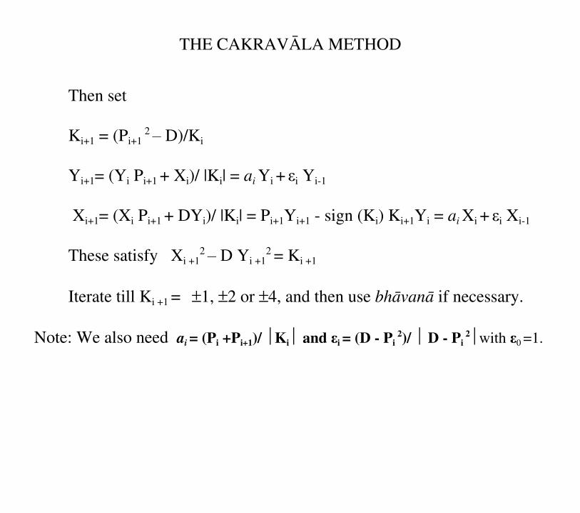
In his letters to Goldbach in 1753 and 1755 Euler speaks of certain improvements he had made in the “Pellian method”.
In a paper, read in 1759 but published in 1765 (1767), entitled “De Usu novi algoritmi in problemate Pelliano solvendo” Euler describes the method of solving X2 –D Y2 = 1 by the simple continued fraction expansion of √D. He gives a table of cycles (of partial quotients) for all non-square integers from 2 to 120 and also notes their various properties.
In a paper which was published earlier in 1762-3 (1764) Euler proves the bhāvanā principle and called it “Theorema Elegantissimum”.
Euler also wrote a paper in 1773 (published in 1783) on “New Aids” for solving the Pell’s equation, where he describes how the equation can be solved if solution is known for K = -1, 2, -2, 4.
By then, in a set of three papers presented to the Berlin Academy in 1768, 1769 and 1770, Joseph Louis Lagrange (1736-1813) had already worked out the complete theory of continued fractions and their applications to Pell’s equation along with all the necessary proofs.

RELATION WITH CONTINUED FRACTION EXPANSION
A simple continued fraction is of the form (ai are positive integers for i>0)
This is denoted by [a0, a1, a2, a3, ... ] or by
Given any real number α, to get the continued fraction expansion, take
a0 = [α] the integral part of α.
Let α1 = 1/( α – [α]). Then we take a1 = [α1]
Let α2 = 1/( α1 – [α1]). Then we take a2 = [α2], and so on.
a0, a1, a2, .. are called partial quotients; α1, α2, ... are the complete quotients.

RELATION WITH CONTINUED FRACTION EXPANSION
The k-th convergent of the continued fraction [a0, a1, a2, a3, ... ] is given by
Ak/Bk = [a0, a1, a2, a3, ... ,ak]
Ak, Bk satisfy the recurrence relations:
A0 = a0, A1 = a1 a0 + 1,
Ak = ak Ak-1 + Ak-2 for k ≥2
B0 = 1, B1 = a1,
Bk = ak Bk-1 + Bk-2 for k ≥2
The convergents also satisfy
Aj Bj-1 – Aj-1 Bj = (-1)j-1

RELATION WITH CONTINUED FRACTION EXPANSION
Example
149/17 = [8, 1, 3, 4]
The convergents are
A0/B0 = 8/1, A1/B1 = 9/1, A2/B2 =35/4, A3/B3 =149/17
We have
A3 B2 – A2 B3 = 149.4–35.17 = 1
This is very similar to the kuññaka method for solving 149x – 17y =1.
Note: The simple continued fraction expansion of a real number does not
terminate if the number is irrational. For instance
(1+ √5)/2 = [1, 1, 1, 1, ...],
e = [2, 1, 2, 1, 1, 4, 1,1, 6, 1, 1, 8, 1, 1, ...].

RELATION WITH CONTINUED FRACTION EXPANSION
It was noted by Euler that the simple continued fraction of √D is always
periodic and is of the form
where k is the length of the period, and the convergents Ak-1, Bk-1 satisfy
Ak-12 – DBk-1
2 = (-1)k
Further, all the solutions of, X2 – D Y2 = 1 can be obtained by composing (bhāvanā) of the above solution with itself.
These results were later proved by Lagrange.
Example: To solve X2 – 13Y2 = 1
A4/B4 = 18/5 and we have 182 – 13.52 = -1, leading to 6492 – 13.1802 = 1

BHĀSKARA SEMI-REGULAR CONTINUED FRACTIONS
In a couple of papers which appeared during 1938-41, Krishnaswami
Ayyangar showed that the cakravāla procedure actually corresponds to a
“semi-regular continued fraction” expansion of √D.
A semi-regular continued fraction is of the form
a0+ ε1 / a1+ ε2 / a2+ ε3 / a3+ ...
where εi = ± 1, ai ≥ 1 for i≥ 1, and ai + εi+1 ≥ 1 for i≥ 1.
Then the convergents satisfy the relations
A0 = a0, A1 = a1 a0 + ε1,
Aj = aj Aj-1 + εjAj-2 for j ≥2
B0 = 1, B1 = a1,
Bj = aj Bj-1 + εjBj-2 for j ≥2

BHĀSKARA SEMI-REGULAR CONTINUED FRACTIONS
Krishnaswami Ayyangar showed that the cakravāla method of Bhāskara corresponds to a periodic semi-regular continued function (Nearest Square Continued Fraction) expansion
√D = a0+ ε1 / a1+ ε2 / a2+ ε3 / a3+ ...
where ai = (Pi +Pi+1)/ ⏐Ki⏐, εi = (D - Pi 2)/ ⏐ D - Pi
2⏐ and the convergents are
related to the solutions Aj = Xj+1 and Bj = Yj+1.
Note: The Simple Continued Fraction of Euler-Lagrange and the Nearest Integer Continued Fraction can also be generated by a cakravāla type of algorithm if we replace the condition II respectively by
(II') D - Pi +1 2 > 0 and is minimum
(II'') ⏐Pi+1 -√D⏐ is minimum
[The Nearest Integer Continued Fraction expansion is implicit in the variant of the cakravāla method discussed by Nārāyaõa Paõóita in his Gaõitakaumudī (c.1356). It was discovered as a more optimal method for solving "Pell’s equation" than SCF by B. Minnigerode in 1873]

EULER-LAGRANGE METHOD FOR X2 – 67 Y2 = 1
I Pi Ki
ai εi Xi Yi
0 0 1 8 1 1 01 8 -3 5 1 8 12 7 6 2 1 41 53 5 -7 1 1 90 114 2 9 1 1 131 165 7 -2 7 1 221 276 7 9 1 1 1678 2057 2 -7 1 1 1899 2328 5 6 2 1 3577 4379 7 -3 5 1 9053 1106
10 8 1 16 1 48842 5967
The steps which are skipped in cakravāla are highlighted
The corresponding simple continued fraction expansion is
The Bhāskara nearest square continued fraction is given by

EULER-LAGRANGE METHOD FOR X2 – 61 Y2 = 1
I Pi Ki
ai εi Xi Yi
0 0 1 7 1 1 01 7 -12 1 1 7 12 5 3 4 1 8 13 7 -4 3 1 39 54 5 9 1 1 125 165 4 -5 2 1 164 216 6 5 2 1 453 587 4 -9 1 1 1070 1378 5 4 3 1 1523 1959 7 -3 4 1 5639 722
10 5 12 1 1 24079 308311 7 -1 14 1 29718 3805
The steps which are skipped in cakravāla are highlighted

EULER-LAGRANGE METHOD FOR X2 – 61 Y2 = 1 (CONTD)
12 7 12 1 1 440131 5635313 5 -3 4 1 469849 6015814 7 4 3 1 2319527 29698515 5 -9 1 1 7428430 95111316 4 5 2 1 9747967 124809817 6 -5 2 1 26924344 344730918 4 9 1 1 63596645 814271619 5 -4 3 1 90520989 1159002520 7 3 4 1 335159612 4291279121 5 -12 1 1 1431159437 18324118922 7 1 14 1 1766319049 226153980
The corresponding simple continued fraction expansion is
The Bhāskara nearest square continued fraction is given by

BHĀSKARA OR NEAREST SQUARE CONTINUED FRACTION
In the continued fraction development of √D, the complete quotients are quadratic surds which may be expressed in the standard form (P +√D)/Q, where P, Q and (D-P2)/Q are integers prime to each other.
If a = [(P +√D)/Q] is the integral part of (P +√D)/Q, then we can have
(P +√D)/Q = a + Q'/( P' +√D) (I)
(P +√D)/Q = (a +1) - Q''/( P'' +√D) (II)
where the surds in the rhs are also in the standard form.
In the Bhāskara or Nearest Square Continued Fraction development we choose a as the partial quotient
(i) if ⏐P'2-D⏐<⏐P''2-D⏐,
ii) or if ⏐P '2-D⏐=⏐P' '
2-D⏐ and Q<0. Then we set ε = 1.
Otherwise we choose a +1 as the partial quotient and set ε = -1.
Note: If we start with √D, we always have Pi ≥ 0 and Qi >0 and Ki = (-1)i ε1 ε2... εi Qi

BHĀSKARA OR NEAREST SQUARE CONTINUED FRACTION
Krishnaswami Ayyangar showed that the Bhāskara or nearest square continued fraction of √D is of the form
where k is the period. Further, it has the following symmetry properties:
Type I: There is no complete quotient of the form [p+q+√( p2+q2)]/p,
where p>2q>0 are mutually prime integers. In this case, the Bhāskara
continued fraction for √D has same symmetry properties as in the case of
Simple Continued Fraction expansion.

BHĀSKARA OR NEAREST SQUARE CONTINUED FRACTION
Examples of Type I:
Type II: There is a complete quotient of the form [p+q+√( p2+q2) ]/p, where p>2q>0 are mutually prime integers. In such a case, the period k ≥4 and is even and there only one such complete quotient which occurs at k/2. The symmetry properties are same as for Type I, except that
Examples of Type II:

LEHMER ON BHĀSKARA CONTINUED FRACTION
The American number theorist Derrick Henry Lehmer (1905-1991) reviewed the work of Krishnaswami Ayyangar in the Mathematical Reviews (1944):
“These papers are concerned with a peculiar semi-regular continued fraction algorithm somewhat akin to the nearest integer algorithm. The expansion is defined only for the standard quadratic surd... and is presumably based on Bhāskara’s ‘cyclic method’ of solving the Pell equation, although the author does not trace the connection in detail...
The author proves that the period is either symmetric, as in the regular case, or else ‘almost symmetric’, that is symmetric except for three central asymmetric partial quotients...
The theory of this continued fraction in most respects closely parallels the classical regular case of Lagrange. The slight blemishes characteristic of the new (or should one say 12th century) algorithm do not seem to be compensated by any useful features other than that possessed by the nearest integer algorithm....”

RECENT WORK ON "PELL’S EQUATION"
"Pell’s equation" continues to be an important subject of current research.
The period k(D) of the simple continued fraction expansion of √D is a good measure of the number of steps needed to solve the equation. And this is known to fluctuate wildly between as low a value as 1 and an upper bound which is of the order of (√D)log(D). The solutions are similarly bounded above by a multiple of D exp(√D)
For instance, for D=1620, k(D) = 1 and we have the roots (161, 4)
For D=1621, k(D) = 78 (the NSCF has a period of 56), and the larger root has 76 digits!
While it is true that even writing down the solutions involves exponential time (in terms of input length logD), various algebraic number theoretic techniques are being developed to obtain a significant number of digits of the solution by "faster" means. Recently Hallgren (2002) has come up with a polynomial-time quantum algorithm for the same purpose.
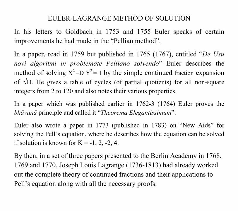
MID-POINT CRITERIA
Recently, Mathews, Robertson and White (2010) have worked out the mid-point criteria for the Bhāskara continued fraction expansion of √D.
In the case of the Simple Continued Fraction expansion of √D, the mid-point criteria were given by Euler:
If Qh-1 = Qh (or ⏐Kh-1⏐= ⏐Kh⏐), then the period k = 2h-1 and
Ak-1 = Ah-1Bh-1+ Ah-2Bh-2
Bk-1 = Bh-12 + Bh-2
2
which satisfy Ak-12 - DBk-1
2 = -1
If Ph = Ph+1, then the period k = 2h and
Ak-1 = Ah-1Bh+ Ah-2Bh-1
Bk-1 = Bh-1 (Bh + Bh-2)
which satisfy Ak-12 - DBk-1
2 = 1

MID-POINT CRITERIA
Mathews et al have obtained the following mid-point criteria for the Bhāskara or the Nearest Square Continued Fraction expansion of √D:
If Qh-1 = Qh (or ⏐Kh-1⏐= ⏐Kh⏐), then the period k = 2h-1 and
Ak-1 = Ah-1Bh-1+ εhAh-2Bh-2
Bk-1 = Bh-12 + εhBh-2
2
which satisfy Ak-12 - DBk-1
2 = -εh
If Ph = Ph+1, then the period k = 2h and
Ak-1 = Ah-1Bh+εh Ah-2Bh-1
Bk-1 = Bh-1 (Bh + εhBh-2)
which satisfy Ak-12 - DBk-1
2 = 1
In the Type I case, the mid-point will in variably satisfy one of the above two criteria.

MID-POINT CRITERIA
In the Type II case, the following is the mid-point criterion:
When Qh = ⏐Kh⏐ is even and Ph = Qh + (½)Qh-1 = ⏐Kh⏐+ (½)⏐Kh-1⏐ and εh =1, then k = 2h and
Ak-1 = AhBh-1- Bh-2 (Ah-1 - Ah-2)
Bk-1 = 2Bh-12 - Bh Bh-2
which satisfy Ak-12 - DBk-1
2 = 1
These mid-point criteria serve to further simplify the computation of the solution.
Note: The mid-point criteria for the Nearest Integer Continued Fraction expansion, obtained by Williams and Buhr (1979), are considerably more complicated than the above mid-point criteria for NSCF.
OPTIMALITY OF CAKRAVĀLA METHOD
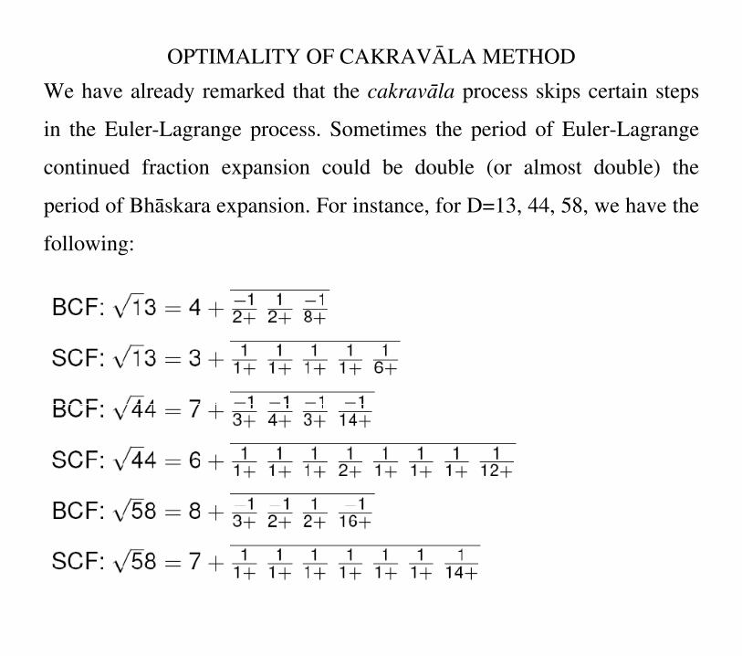
We have already remarked that the cakravāla process skips certain steps
in the Euler-Lagrange process. Sometimes the period of Euler-Lagrange
continued fraction expansion could be double (or almost double) the
period of Bhāskara expansion. For instance, for D=13, 44, 58, we have the
following:

OPTIMALITY OF CAKRAVĀLA METHOD
We may note that whenever there is a 'unisequence' (1,1,...,1) of partial
quotients of length n, the cakravāla process skips exactly (n/2) steps if n is
even, and (n+1)/2 steps if n is odd.
In a series of papers (1960-63), Selenius has shown that the cakravāla
process is 'ideal' in the sense that, whenever there is such a 'unisequence',
only those convergents Ai/Bi are retained for which Bi⏐Ai - Bi √D ⏐ are
minimal.
Recently, Mathews et al (2010) have shown that the period of Bhāskara or
Nearest Square Continued Fraction is the same as that of the Nearest
Integer Continued Fraction. They also estimate that the ratio of this period
to that of simple continued fraction is log2 [(1+√5)/2] ≈ 0.6942419136...

OPTIMALITY OF CAKRAVĀLA METHOD

REFERENCES 1. Bījagaõita of Bhāskara with Comm. of Kçùõa Daivajña, Ed.
Radhakrishna Sastri, Saraswati Mahal, Thanjavur 1958. 2. Bījagaõita of Bhāskara with Vāsanā and Hindi Tr. by Devachandra Jha,
Chaukhambha, Varanasi 1983. 3. Bījagaõita of Bhāskara with Vāsanā, with notes by T. Hayashi,
SCIAMVS, 10, December 2009, pp. 3-303. 4. H. T. Colebrooke, Algebra with Arithmetic and Mensuration from the
Sanskrit of Brahmagupta and Bhāskara, London 1817. 5. J. Wallis, Commercium Epistolicum de Quaestionibus, London, 1658. 6. L. Euler, Elements of Algebra with Notes of Bernoulli and Lagrange,
Tr. by J. Hewlett, 3ed 1822. 7. B. Minnegerode, Uber eine neue methode die Pellsche Gleischung
aufzullosen, Nachr Konig Gesselsch Wiss Gottingen Math Phys Kl, 23, 1873, pp. 619-652.
8. A. Hurwitz, Uber eine besondere Art de Kettenbruchentwicklung Grossen, Acta Math. 12, 1889, pp.367-405.
9. A. A. Krishnaswami Ayyangar, New Light on Bhāskara’s Cakravāla or Cyclic method, J. Indian Math. Soc. 18, 1929-30, pp.225-248.

10. B. Datta and A. N. Singh, History of Hindu Mathematics, Vol II, Algebra, Lahore 1938; Reprint, Asia Publishing House, Bombay 1962.
11. A. A. Krishnaswami Ayyangar, A New Continued Fraction, Current Sci., 6, June 1938, pp. 602-604.
12. A. A. Krishnaswami Ayyangar, Theory of Nearest Square Continued Fraction, J. Mysore Univ., Section A 1, 1941, pp 21-32, 97-117.
13. K. S. Shukla, Acharya Jayadeva the Mathematician, Ganita, 5, 1954, pp.1-20.
14. C. O. Selenius, Rationale of the Cakravāla Process of Jayadeva and Bhāskara II, Hist. Math. 2, 1975, pp.167-184.
15. H. C. Williams and P. A. Buhr, Calculation of the regulator of
Q (√D) by the use of the Nearest Integer Continued Fraction algorithm, Mathematics of Computation, 33, 1979, pp.369-381.
16. A. Weil, Number Theory An Approach Through History From Hammurapi to Legendre, Birkhauser, Boston 1984.
17. R. Sridharan, Ancient Indian Contributions to Quadratic Algebra, in B. V. Subbarayappa and N. Mukunda Eds., Science in the West and India, Himalaya, Bombay 1995, pp.280-289.

18. H. C. Williams, Solving the Pell’s equation, in M. A. Bennett et al Eds., Proc. of Millennial Conference on Number Theory, A. K. Peters, Mass. 2002, pp. 397-435.
19. H. W. Lenstra Jr., Solving the Pell’s equation, Notices of Amer. Math. Soc. 49, 2002, pp. 182-192.
20. S. Hallgren, Polynomial-time Quantum Algorithms for Pell’s equation and the principal ideal problem, STOC 2002.
21. M. S. Sriram, Algorithms in Indian Mathematics, in G. G. Emch et al Eds., Contributions to the History of Indian Mathematics, Hindustan Book Agency, Delhi 2005, pp.153-182.
22. M. J. Jacobson and H. C. Williams, Solving the Pell’s Equation, Springer, New York 2009.
23. K. R. Matthews, J. P. Robertson and J. White, Mid-point Criteria for Solving Pell’s Equation Using the Nearest Square Continued Fraction, Math. Comp. 79, 2010, pp.485-499.
24. K. R. Mathews and J. P. Robertson, Equality of Period Length for NICF and NSCF, Glass. Mat. Ser. III, 46.2, 2011, pp. 269-282.
25. A. Dutta, Nārāyaõa’s Treatment of Varga-prakçti, Indian Journal of History of Science 47, 2012, pp.633-77.