Coastal Engineering 116 (2016) 118–132

Contents lists available at ScienceDirect

Coastal Engineering

j ourna l homepage: www.e lsev ie r .com/ locate /coasta leng

The California coastal wave monitoring and prediction system

W.C. O'Reilly ⁎, Corey B. Olfe, Julianna Thomas, R.J. Seymour, R.T. GuzaIntegrative Oceanography Division, Scripps Institution of Oceanography, University of California, San Diego, La Jolla, CA, United States

⁎ Corresponding author at: Integrative OceanographStudies - 0209, Scripps Institution of Oceanography, Uni9500 Gilman Drive, La Jolla, CA 92093-0209, United State

E-mail addresses: woreilly@ucsd.edu (W.C. O'Reilly), cjothomas@ucsd.edu (J. Thomas), rseymour@ucsd.edu (R.J(R.T. Guza).

http://dx.doi.org/10.1016/j.coastaleng.2016.06.0050378-3839/© 2016 The Authors. Published by Elsevier B.V

a b s t r a c t

a r t i c l e i n f o

Article history:Received 26 January 2016Received in revised form 20 May 2016Accepted 11 June 2016Available online 6 July 2016

A decade-long effort to estimate nearshore (20 m depth) wave conditions based on offshore buoy observationsalong the California coast is described. Offshore, deep water directional wave buoys are used to initialize a non-stationary, linear, spectral refraction wave model. Model hindcasts of spectral parameters commonly used innearshore process studies and engineering design are validated against nearshore buoy observations seawardof the surfzone. The buoy-drivenwavemodel shows significant skill atmost validation sites, but prediction errorsfor individual swell or sea events can be large.Model skill is high in north San Diego County, and low in the SantaBarbara Channel and along the southernMonterey Bay coast. Overall, the buoy-drivenmodel hindcasts have rel-atively low bias and therefore are best suited for quantifying mean (e.g. monthly or annual) nearshore wave cli-mate conditions rather than extreme or individual wave events. Model error correlation with the incidentoffshore wave energy, and between neighboring validation sites, may be useful in identifying sources of regionalmodeling errors.

y Diviversitys.olfe@u. Seymo

. This i

© 2016 The Authors. Published by Elsevier B.V. This is an open access article under the CC BY license(http://creativecommons.org/licenses/by/4.0/).

Keywords:Ocean wavesWave buoysWave modelsWave refractionWave runupLongshore radiation stress

1. Introduction

Spectral wave energy and radiation stresses, just prior to depth-limited wave breaking in the surfzone, are critical boundary conditionsfor modeling nearshore circulation, wave runup, and sediment trans-port. However, nearshore wave spectra in California often vary on rela-tively short longshore length scales [O(few wavelengths)] , owing tocomplex shelf bathymetry, making it impossible to measure directlythe regional nearshore wave climate using existing measurement tech-nology. Therefore, validated models for nearshore waves are importantwhen managing nearshore hazards at both short and long time scales(e.g. 2 day to 50 year forecast scenarios of coastal flooding).

Nearshore waves in California are typically estimated using a Pacificocean-scale wind-wavemodel (e.g.Wavewatch-III, Chawla et al., 2013)as a boundary condition for a “nested” coastal wind-wave hindcastmodelwhich resolveswavelength-scale shallowwater bathymetric fea-tures (e.g. SWAN, Rogers et al., 2007; Adams et al., 2008; Van derWesthuysen et al., 2013, Barnard et al., 2014). The bias and skill of near-shore wind-wave hindcasts has improved significantly with improve-ments in the offshore boundary conditions (frequency-directionalspectra) from the deep water wind-wave models, particularly in theswell frequency bands in the Pacific (Hanson et al., 2009). Nevertheless,

sion, Center for Coastalof California, San Diego,

csd.edu (C.B. Olfe),ur), rguza@ucsd.edu

s an open access article under

challenges remain owing to the sensitivity of annual longshore wave-drivenmass flux to a small bias in the nearshore wave direction param-eters and the availability of historical high resolution coastal wind fieldboundary conditions (Rasmussen et al., 2009). Assimilating buoy mea-surements intowind-wavemodel hindcasts is an area of active research(Orzech et al., 2013; Panteleev et al., 2015), but in engineering practicenearshore buoys are mostly used for hindcast validation.

Here, in contrast to initializing a coastal wind-wave model with anocean-scale model, a network of deep water directional buoy measure-ments are used to initialize a linear wave propagation model. The com-putationally fast model estimates nearshore wave energy and low-order directional spectra moments with O(1 wavelength) alongshoreresolution. Future work combines offshore buoys and global scalemodels to improve the initialization of local models.

The California buoy array is described in Section 2. In Section 3, theMaximum Entropy Method (Lygre and Krogstad, 1986) is used to esti-mate hourly frequency-directional spectra at offshore deep water buoys,providing boundary conditions for a non-stationary linear wave propaga-tionmodel (Pierson et al., 1952; Longuet-Higgins, 1957;Dorrestein, 1960;LeMehaute and Wang, 1982; O'Reilly and Guza, 1991, 1993, 1998). Thespectrum is split into swell (f = 0.0375–0.0875 Hz) and sea (f =0.0875–0.5 Hz) bands. For each nearshore prediction point, directionalspectra estimates from multiple offshore buoys are combined with aweighting that depends on the frequency band, deep water wave direc-tion and prediction buoy location (Appendix B).

In Section 4, the buoy-driven prediction methodology is validatedwith nearshorewave observations at 13 shallow(~20mdepth) sites. Pre-diction accuracy (R2 skill, bias and rms error) is assessed for totalwave en-ergy, the centroid frequency, the peak frequency, and themean direction.

the CC BY license (http://creativecommons.org/licenses/by/4.0/).

119W.C. O'Reilly et al. / Coastal Engineering 116 (2016) 118–132

The model performs best in the southern section of the Southern Califor-nia Bight (San Clemente Basin), poorly in the Santa Barbara and San PedroChannel regions, and moderately well elsewhere.

The potential utility of the nearshore hindcast in practical coastal en-gineering applications is examined in Section 5. Predictions of thelongshore radiation stress, Sxy, the principal driver of alongshore sedi-ment transport, validate well in north San Diego and Orange Countiesfor a given shore normal direction. However, uncertainty in definingthe local shoreline normal creates significant Sxy uncertainty.

The peak frequency, fp, a commonly used parameter in empiricalwave runup formulas (Stockdon et al., 2006), is shown to be unstablein southern California when sea and swell peak energies are similar.

In Section 6, long concurrent records from southern California buoys,sheltered from incident swell by the offshore Channel Islands, are usedto examine the source of model error in the swell band. At some shel-tered buoys, errors correlate most strongly with conditions offshore ofthe Channel Islands, while errors at other buoys are more highly corre-lated with errors at adjacent buoys. Section 7 is a summary.

2. Wave monitoring: the California Directional Wave Buoy network

Anetwork of 17Waveriders atfixed deepwater locationsmonitoredincident deep water wave conditions in three relatively highly populat-ed coastal regions; southern California (U.S. Mexico border to MorroBay), central California (Big Sur to Bodega Bay) and northern California(Humboldt Bay Area). Six buoys weremoored well offshore, seaward of

Fig. 1. Locations of buoys used to predict and validate nearshore wave parameters along the(NOAA 3 m discus buoys).

islands and shoals, to monitor incident swell (squares in Fig. 1), and 11buoys were moored near the mainland shelf break to monitor locallygenerated seas and validate the swell model. These observations arecombined to predict sea and swell at nearshore locations along themainland coast (Section 3). The deployment periods ranged from 5 to14 years, all between 2001 and 2014 (Tables 1, 2).

Waveriders are translational buoys that measure accurately the seasurface position (x, y and z) of swell (O'Reilly et al., 1996). Every half-hour, on-board analysis yields estimates of the wave energy, a0, andlowest order moments of the directional wave spectrum S(f,θ) at eachfrequency, retained as normalized directional Fourier coefficients a1,b1, a2, and b2 (e.g., Kuik et al., 1988).

Hourlywave energy and directional Fourier coefficients are obtainedby merging half-hourly records, the directional coefficients aresmoothed with a 3-hour running mean filter, and a directional estima-tor is used tomake hourly S(f,θ) wavemodel input spectra. Different es-timators use different optimizing criteria (e.g., maximum directionalsmoothness, maximum entropy). The Maximum Entropy Method(MEM, Lygre and Krogstad, 1986) used here fits the measured direc-tional coefficients exactly, eliminating any possibility of time-averagedestimator bias in the resulting directional distribution moments, com-pared to the original observations. MEM also produces narrow direc-tional peaks. These are desirable estimator attributes for wave climateestimation on a swell-dominated coast.

CDIPWaverider buoy stations in shallowwater, usually deployed fora few years, are used to validate the prediction methodology (Table 3).

California coast. All buoys are Datawell Directional Waveriders, except 46022 and 46026

Table 1Time periods of offshore deep water buoys (black squares, Figs. 1 and 2) used for nearshore model validation (Table 3).

Offshore station Validation time period Water depth (m) Location

Cape Mendocino 06/2005–04/2013 334 40.294 N 124.740 WPoint Reyes 07/2007–06/2013 550 37.938 N 123.063 WPoint Sur 05/2009–11/2014 366 36.341 N 122.102 WHarvest 01/2000–11/2014 548 34.458 N 120.782 WSan Nicolas Island 01/2000–11/2014 307 33.221 N 119.882 WPoint Loma South 10/2007–11/2014 1143 32.530 N 117.431 W

120 W.C. O'Reilly et al. / Coastal Engineering 116 (2016) 118–132

Most of the shallow southern California buoys are on relatively uncom-plicated sandy stretches of coastline specifically selected for testing themodel applicability for generic beach process studies. The few near-shore buoys in central and northern California were deployed forother applications, and severe local bathymetric features make themsuboptimal for general model testing. Most of the nearshore wave pre-dictions useWaverider observations (Fig. 1), but observations from theNational Data Buoy Center (NDBC) 3 m discus buoys were sometimesused to fill data gaps, particularly for the local seas in central and north-ern California (e.g. 46,026 in Fig. 1). CDIP buoy stations used in thisstudy are listed in Tables 1–3.

3. Wave prediction: a non-stationary linear spectral refractionmodel

A backward ray-tracing linear spectral refraction model (Piersonet al., 1952; Longuet-Higgins, 1957; and Dorrestein, 1960) is used to es-timate the transformation of wave spectra from deep water buoy sta-tions to nearshore prediction points. Spectral refraction was first usedto study California swell by Munk et al. (1963), and later byLeMehaute and Wang (1982); O'Reilly and Guza (1991, 1993), andothers.

Spectral refraction accounts for island blocking, wave refraction, andwave shoaling. It has been validated in Southern California (O'Reilly andGuza, 1993; O'Reilly and Guza, 1993; Rogers et al., 2002) and is wellsuited for the U.S. West Coast, where the continental shelf is steep andnarrow, and bottom dissipation is believed small (García-Medinaet al., 2013). In steady conditions, the deep water spectrum, So(f,θo),and the wave spectrum at a shallow location, S(f,θ), are related by.

S f ; θð Þ ¼ k fð ÞCgo fð Þko fð ÞCg fð Þ So f ; θoð Þ where; θo ¼ Γ f ; θð Þ ð1Þ

The subscript, o, refers to the incident wave spectrum in deepwater,k is the scalar wave number and Cg the group velocity for a given wavefrequency and water depth based on the linear dispersion relation.Eq. (1) is valid along a ray path, and Γ, the relationship between θ andθo, is obtained by back-refracting wave rays from the shallow or

Table 2Time periods of local deep water buoys (black triangles, Figs. 1 and 2) used for nearshore mod

Local deep water station Validation time period

NOAA 46022 06/2005–04/2013North Spit 02/2010–04/2013NOAA 46026 07/2007–06/2013Mty. Canyon Outer 05/2009–11/2014Goleta 06/2002–11/2014Anacapa 06/2002–11/2014Santa Monica 01/2000–11/2014San Pedro 01/2000–11/2014Dana Point 07/2000–11/2014Oceanside 09/2005–11/2014Torrey Pines 01/2001–11/2014

sheltered site (e.g., Figs. 1–3, O'Reilly and Guza, 1991). LeMehaute andWang (1982) refer to Γ as the inverse direction function.

Unsteady conditions are modeled by introducing time, t, and a timelag τ. Model initialization uses n deep water buoys with weightingfunction w.

S f ; θ; tð Þ ¼XN

n¼1

k fð ÞCgo fð Þko fð ÞCg fð ÞSo;n f ; θo; t þ τ f ; θoð Þ½ � �w n; θoð Þ; θo

¼ Γ f ; θð Þ; ð2Þ

where the time lag, τ(f,θo), is estimated based on the idealized deepwater path of a wave group front arriving from the direction θo andpassing through the deep water buoys and nearshore prediction loca-tions (Appendix B, Fig. B1). The weighting function w(n,θo) for buoy nis based on the proximity distance, dn, of the buoy to the θo great circlepath passing through the prediction site. For a given deep water direc-tion, themore directly “upwave” or “downwave” a buoy is to the predic-tion site, the higher the weight relative to the other deep water buoys(see Appendix B, Fig. B1),

w n; θoð Þ ¼ d−1nXN

i¼1d−1i

ð3Þ

A maximum of N = 2 buoys, the highest weighted upwave anddownwave buoys, are used for each θo arrival direction in Eq. (3). Forswell prediction, w(θo) is also used to restrict buoy estimates of S(θo)to the plausible range of directions for pacific swell arrivals by settinglandward directions of w(θo) = 0. Using multiple buoys for boundaryconditions allows continuous nearshore predictions when some buoysare inoperable. Eq. (2) yields a linear transformation of time series ofdeep water directional spectra to time series of wave energy or any di-rectional moment of the nearshore wave spectra,

Zθ

S f ; tð Þmpdθ ¼

XNn¼1

k fð ÞCgo fð Þko fð ÞCg fð Þ

Zθ

so;n f ; Γ f ; θð Þ; t þ τð f ; Γ f ; θð ÞÞ½ �w n; Γ f ; θð Þð Þmpdθ;

ð4Þ

el validation (Table 3).

Water depth(m) Location

680 40.744 N 124.575 W168 40.888 N 124.357 W53 37.755 N 122.839 W156 36.761 N 121.947 W182 34.333 N 119.803 W114 34.167 N 119.435 W363 33.855 N 118.633 W457 33.618 N 118.317 W370 33.458 N 117.767 W220 33.179 N 117.471 W549 32.930 N 117.392 W

Table 3Time periods of nearshore buoy validations (black circles, Figs. 1 and 2).

Nearshore station Validation time period Water depth(m) Location

South Spit 06/2005–04/2013 40 40.753 N 124.313 WSan Francisco Bar 07/2007–06/2013 15 37.787 N 122.634 WCabrillo Point 05/2009–11/2014 18 36.626 N 121.907 WDiablo Canyon 01/2000–11/2014 23 35.204 N 120.859 WRincon Point 09/2005–04/2007 21 34.356 N 119.475 WPitas Point 10/2004–09/2005 20 34.317 N 119.417 WPort Hueneme 04/2007–02/2009 20 34.100 N 119.167 WLeo Carillo 04/2003–03/2004 20 34.033 N 118.917 WHuntington Beach 06/2005–11/2006 22 33.623 N 118.012 WCamp Pendleton 01/2008–11/2014 20 33.220 N 117.439 WSan Elijo 04/2009–06/2012 20 33.003 N 117.292 WTorrey Pines Inner 04/2001–03/2004 20 32.929 N 117.273 WImperial Beach 12/2006–01/2010 18 32.569 N 117.169 W

121W.C. O'Reilly et al. / Coastal Engineering 116 (2016) 118–132

p=1,2,3,4,5 where m1(θ)=1,m2(θ)= cosθ ,m3(θ)= sinθ ,m4(θ)=cos2θ ,m5(θ)= sin2θ ,…Eq. (4) is piece-wise integrated for discretebandwidths of θo ,where θo=Γ(f,θ), to derive a linear system of equa-tions for the transformation of discrete deepwater spectra to nearshoreenergy and directional moments (O'Reilly and Guza, 1998),

b ¼ A � So ð5Þ

Thematrix b of total wave energy and directionalmoments at a shel-tered site is related to the energy in discrete frequency-direction bins(Δf,Δθo) of the offshore spectra, So, by a forward model transformationmatrix A. Each element of A is derived from the right-hand side ofEq. (5), which is integrated over discrete segments of the inverse direc-tion function Γ(f,θ) that fall within the range of eachΔθo deepwater di-rection band.

To predict the nearshore wave spectrum using deep water buoys, thespectrum is split into swell (f= 0.0375–0.0875 Hz) and sea (f= 0.0875–0.5 Hz) components. The swell component (also known as ground swell)has distant sources, and offshore boundary conditions are applied

Fig. 2. Locations of buoys used to predict and validate nearshore wave parameters in the SouthWaveriders.

seawards of islands and shoals (black squares, Figs 1 and 2). The sea com-ponents (also known aswind swell, chop, and local seas), generated clos-er to the coastline, are predicted using buoys nearer the coast, but still indeep water for waves in this frequency range (black triangles, Figs 1 and2). The 0.0875 Hz cutoff between the sea and swell bands is based on thesharp decrease in observed swell energy at 0.08–0.10 Hz in the dispersivearrivals of swell from distant storms (e.g. Munk et al., 1963).

4. Model validation

An important purpose of the buoy network is to provide wave inputto nearshore coastal process models (surfzone circulation, runup, andsediment transport). Therefore, the validation parameters are basedon the aspects of nearshore waves important to nearshore processes:wave energy (E), the first moment (the centroid, fc) of the frequencyspectrum, and the mean direction of second moment of the directionalspectrum (θ2) (critical to estimatingwave radiation stresses). Two addi-tional common validation parameters, significant wave height (Hs) andthe peak wave frequency (fp), are also presented (Appendix A).

ern California (shaded line is the 300 m depth contour). All buoys are Datawell Directional

Fig. 3.Model R2 prediction skill (a.) and bias (b.) for energy (top panels), centroid frequency (middle panels), and the bulk 2ndmomentmean direction (bottompanels) at all the Californianearshore validation buoys (north to south), for swell (squares), seas (triangles), and the combined total spectrum(circles).

122 W.C. O'Reilly et al. / Coastal Engineering 116 (2016) 118–132

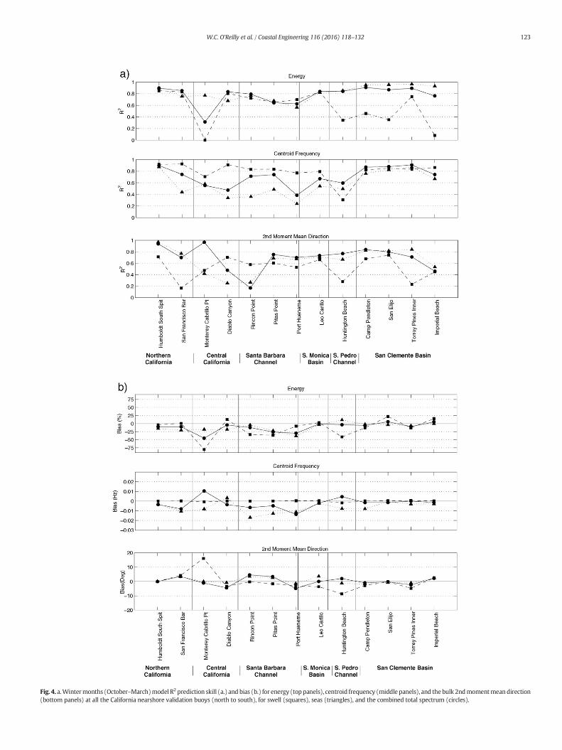
Fig. 4. a.Wintermonths (October–March)model R2 prediction skill (a.) and bias (b.) for energy (top panels), centroid frequency (middle panels), and the bulk 2ndmomentmeandirection(bottom panels) at all the California nearshore validation buoys (north to south), for swell (squares), seas (triangles), and the combined total spectrum (circles).

123W.C. O'Reilly et al. / Coastal Engineering 116 (2016) 118–132

124 W.C. O'Reilly et al. / Coastal Engineering 116 (2016) 118–132

However, in California, the observed and modeled fp is sometimes un-stable, jumping between sea and swell peaks of similar energy(Section 5.2).

Frequency integrated, predictions of bulkwave parameters are, fromEq. (5),

E tð Þ ¼Zf

Zθ

S f ; tð Þdθdf ;

f c tð Þ ¼Zf

Zθ

f � S f ; tð Þdθdf�Z

f

Zθ

S f ; tð Þdθdf ;

θ2 tð Þ ¼ 12arctan

Z Zf ;θS f ; tð Þ sin2θdθdf

�Z Zf ;θS f ; tð Þ cos2θdθdf

� �;

ð6Þ

where f is integrated over the swell bands, sea bands, or all frequencies.Hourly predictions (Eqs. (3) and (4)) are compared with concurrenthourly nearshore buoy observations. Model performance is assessedwith: the R-squared coefficient of determination, or model skill,

R2 ¼ 1−∑ pred�obsð Þ2.∑ obs−obs

� �2

bias ¼ 1N∑

N

1pred�obsð Þ

and bias removed root‐mean‐square errors

RMSE ¼ffiffiffiffiffiffiffiffiffiffiffiffiffiffiffiffiffiffiffiffiffiffiffiffiffiffiffiffiffiffiffiffiffiffiffiffiffiffiffiffiffiffiffiffiffiffiffiffiffiffiffiffiffiffiffiffiffiffiffiffiffiffiffiffi1

N−1∑N

1pred�obs−biasð Þ2

rð7Þ

Annual model skill and bias at the nearshore buoys (Figs. 1 and 2,Table 3) are summarized in Fig. 3 (Appendix A has tabulated values),and shown seasonally (winter vs. summer months) in Figs. 4 and 5.For the year-round, total spectrum energy hindcasts (black circles,upper panel, Fig. 3a, b), the buoy-driven model shows the best near-shore hindcast skill in the San Clemente Basin section of southern Cali-fornia (R2 N 0.9; bias b 10%). Skill is lower (R2 b 0.8) and bias higher(N15%) on the south shore of Monterey Bay, and at the east end of theSanta Barbara Channel. Elsewhere, skill and bias are moderate (0.8 b

R2 b 0.9; bias b 15%). Centroid frequency and 2ndmoment mean direc-tion hindcasts showed similar regional performance patterns (black cir-cles, middle and bottom panels, Fig. 3a, b), but with lower average skillsthan energy. R2 can be a negative number, when the bias error exceedsthe standard deviation of the observations, and is plotted as zero skill(e.g. Monterey Cabrillo Point swell skill, Fig 3a).

When decomposed into sea and swell components (black trianglesand squares, Fig. 3a, b), the model performance becomesmore nuancedfor the San Clemente Basin nearshore sites. Swell predictions remainunbiased, but swell energy prediction skill is relatively poor (0.4 b

R2 b 0.8, black squares, upper panel, Fig. 3a). The total spectrum skill ishigh owing to the very high skills for seas (black triangles, upperpanel far right, Fig. 3a). Further decomposed into seasons, San ClementeBasin swell energy skill is particularly low in winter (black squares,upper panels, Figs. 4a and 5a), with R2 ≈ 0.25 at Imperial Beach. Theshelf bathymetry to the south of the Imperial Beach area is of lowerquality than elsewhere, and is believed partially responsible for thelow summer R2. Results are improved (not shown) using alternative ba-thymetry from undocumented sources.

For seas, the centroid frequency, fc, hindcast skill is poor and biasedlow throughout California, with the exception of the San ClementeBasin (black triangles, middle panels, Fig. 3a, b), and the 2nd momentmean direction of the local seas is poorly hindcast in central California(bottom panel, Fig. 3a, b). The lowest fc skill is in winter, while the sea2ndmomentmean direction skill is lowest in summer (Figs. 4a and 5a).

5. Coastal engineering applications

The buoy-driven model provides relatively unbiased yearly esti-mates of the important nearshore spectral wave parameters, for exam-ple along the San Clemente Basin mainland coast (black dots, right-hand side of panels in Fig. 3b). Here, buoy-driven regional modelhindcasts of longshore sediment transport and wave runup are com-pared with estimates using a nearshore buoy.

5.1. Longshore transport

In coastal engineering design and regional sediment managementstudies, it is typically assumed that the longshore sediment volumeflux, Qy, is linearly related to the total incident wave energy, E, andthe longshore wave radiation stress, Sxy (Seymour and Higgins, 1978;USACE, 1984),

Qy �ffiffiffiffiffiffiHs

p� Sxy � E1=4 � Sxy ð8Þ

The longshore radiation stress is an integral property of the seconddirectional moment of the incident wave spectrum just prior to wavebreaking,

Sxy ¼ 12

Zf

Zθ

cg fð Þc fð Þ S f ; θð Þ sin2 θ−θnð Þdfdθ ð9Þ

where cg and c are the wave group and phase speeds respectively.The sine second directional moment is calculated relative to the

shoreline normal, θn, perpendicular to the assumed parallel nearshoredepth contours. The predicted Sxy uses the model S(f,θ) in Eq. (9)while the nearshore buoy measures the second moment (Eq. (9)) di-rectly. Model skill, bias and root mean square errors for hourly Sxy pre-dictions at five nearshore buoys, located on relatively straight sandysections of the San Clemente Basin and San Pedro Channel mainlandcoast, are shown in Table 4. For each nearshore buoy site, a local esti-mate of θn (based on the orientation of the 10 m depth contour) wasused in both the local buoy and regional model Sxy. Model skill is good(0.8 b R2 b 0.9) at Huntington Beach, Camp Pendleton, and San Elijo,with poorer skill at Torrey Pines and Imperial Beach.

Alongshore sediment transport studies, particularly those associatedwith regional sediment management, are often concernedwithmonth-ly, seasonal, and annual time scales. Monthly mean Sxy (Fig. 6) agreesmuch better than the hourly values, consistentwith the smallmodel en-ergy and direction bias in this region (Fig. 3b, top and bottom). At Hun-tington Beach, Camp Pendleton and San Elijo, the model error(difference between the solid and dashed lines) is relatively small. Addi-tionally, the sign of the observed and modeled annual Sxy are not sensi-tive to a ±5° θn rotation (errors bars in Fig. 6). In these areas, the buoy-driven nearshore Sxy hindcast's seasonal and annual mean “signal” islarger than the likely “noise” owing to local shore normal uncertainty.

At Torrey Pines and Imperial Beach, Sxy is weaker in general, the an-nual average (modeled and observed) can have either sign (±5° scatterbars, far right, Fig. 6). In these cases, shore normal estimation methodsand assumptions (e.g. alongshore and time variation of θn) likely playa more important role in practical, long term, longshore sediment fluxcalculations.

5.2. Wave runup

Stockdon et al. (2006) defines the highest 2% runup exceedance ele-vation, R2, as

R2 ¼ 1:1 0:35β f H0L0ð Þ12 þH0L0 0:563β2

f þ 0:004� �h i1

2

2

0B@

1CA ð10Þ

Fig. 5. a. Summer months (April–September) model R2 prediction skill (a.) and bias (b.) for energy (top panels), centroid frequency (middle panels), and the bulk 2nd moment meandirection (bottom panels) at all the California nearshore validation buoys (north to south), for swell (squares), seas (triangles), and the combined total spectrum (circles).

125W.C. O'Reilly et al. / Coastal Engineering 116 (2016) 118–132

Table 4Nearshore validation statistics for hourly Sxy (validation time periods listed in Table 3).

Nearshore buoy R2 Mean (cm2) Bias (cm2) RMSE (cm2)

Huntington Beach 0.82 −10 −10 39Camp Pendleton 0.89 −21 −4 34San Elijo 0.80 32 4 28Torrey Pines 0.63 −20 12 35Imperial Beach 0.34 15 −10 45

For each site, Sxy has been calculated relative to an estimate of the local shoreline normal.The mean values are based on the observations. The bias and root mean square errors aremodel errors relative to the observations. Positive Sxy values correspond to northward or“upcoast” directed stress.

126 W.C. O'Reilly et al. / Coastal Engineering 116 (2016) 118–132

where βf is the foreshore slope,H0 the equivalent deepwater significantwave height, and L0 the equivalent deepwaterwavelength based on thepeak wave period, Tp, and

L0 ¼ gT2p

2π: ð11Þ

Isolating theH0L0 wave input parameter in Eq. (10) and replacing L0using Eq. (11),

R2 �ffiffiffiffiffiffiffiffiffiffiffiH0L0

p; or � Tp

ffiffiffiffiffiffiH0

p; or �

ffiffiffiffiffiffiH0

pf p

ð12Þ

where H0 is estimated by reverse (un)shoaling the predicted nearshoresignificant wave height, Hs , based on the nearshore peak frequency fp ,or preferably (as done here), the predicted shallow water frequencyspectrum S(f) is unshoaled to deep water prior to deriving H0 and fp.Model predictions of hourly

ffiffiffiffiffiffiH0

p= f p at the nearshore buoys in CA are

unbiased but relatively poor overall, with R2 values b0.60 and RMSE er-rors exceeding 20% (Table 5).

The lowR2 skill values are largely owing to instability of themodeledand observed fp. Although a common design wave parameter in coastalengineering practice, fp and the corresponding peak period Tp are poordescriptors of multimodal wave frequency spectra. In California, seaand swell peaks with similar energy are common, and fp can vary by afactor of 2–3 depending on whether the sea or swell peak is maximum(black crosses, Fig. 7), resulting in clearly nonphysical factor of 2–3 hour-to-hour fluctuations of R2 runup. Observed fp stability dependson the degrees of freedom (wave record length, sample rate, and fre-quency bandwidths) of the processed spectral data. Therefore, themodel fp predictive skill depends significantly on wave climate (e.g.presence of comparable sea and swell peaks) and data analysis factors(e.g. degrees of freedom) that are unrelated to the wave transformationmodel skill.

For general climatic hindcasts (e.g. estimating runup during dailyhigh tide) at locations where multimodal sea states are common, itwould desirable to use an alternative empirical wave runup equationusing a more stable frequency parameter.

The centroid frequency fc is farmore stable (red circles, Fig. 7), but isheavily weighted by the high frequency (short wavelengths) tails of thespectra. A bulk frequency parameter that is more relevant to runup dy-namics is the frequency of the centroidal wavelength, fcL (green dia-monds, Fig. 7),

f cL ¼ffiffiffiffiffiffiffiffiffiffiffiffig

2πLoc

r; ð13Þ

with the centroidalwavelengthLoc ¼ ∫∫ f ;θLoð f Þ � Sð f Þdθdf =∫∫ f ;θLoð f Þ � dθdf ,and where S(f) is unshoaled to deep water.

The potential utility of fcL in climatic studies is illustrated at the CampPendleton nearshore buoy (Fig. 8) where the bulk of the RMSE error inthe hourly runupwave input parameter, and the source of the low R2, isthe “cloud” of poor predictions for the lower half of the

ffiffiffiffiffiffiH0

p= f p values.

The frequency of the centroid wavelength fcL is more stable, with im-proved R2 (right panel in Fig. 8, skill values in brackets in Table 5). How-ever, fcL should not be used directly with the Stockdon et al. formulas,because fp was used in their model calibration. Instead, a best fit coeffi-cient, Cf, between the twowave input parameters,

ffiffiffiffiffiffiH0

p= f p=C f

ffiffiffiffiffiffiH0

p= f cL

would have to be derived fromdeepwater buoy data prior to using fcL inEq. 10.

Finally, the overall fit at the highest values offfiffiffiffiffiffiH0

p= f p (upper right

corner of left panel, Fig. 8) improves because the largest incident wavefrequency spectra aremore unimodal, and fp is more stable and predict-able. Model predictions atmost nearshore buoys (not shown) also haveconsiderably less scatter in of the largest values of

ffiffiffiffiffiffiH0

p= f p. Thus, these

results do not discourage the use of fp in Stockdon et al. (Eq. 10 above)when estimating design wave runup elevations for the most extremewave events (a primary application of Eq. (10)).

6. Discussion

The buoy-drivenmodelingmethodology was originally developed foruse in concert with beach change studies on long, straight beaches in theSan Clemente Basin region. Particular attention was given to the place-ment of deep water and nearshore buoys for this purpose, and this con-tributes to the relatively high skill in San Diego County. In contrast,nearshore validation buoys in central and northern California were de-ployed for other, often very site-specific purposes, in areas with locallycomplex or rocky shallow water bathymetry. These are demanding sitesto model owing to dependence on local bathymetry or extreme shelter-ing. For example, while the hindcast skill at the Cabrillo Point buoy sitein Monterey Bay is notably poor, with a large underprediction bias andnegligible skill in the swell band, this site is highly sheltered on anortheast-facing rocky section of coast. An earlier, more time limitedcomparison of the buoy-driven hindcast model to wave measurementsfurther east in Monterey Bay, on a sandy more exposed section of thecoastline, yielded better results (Orzech et al., 2010).

The present model validation metrics are more stringent than aretypically used to assesswind-wavehindcastmodel performance. In par-ticular, Sxy depends on the mean direction of the incident wave energyflux relative to shore normal θ−θn immediately seaward of thebreakpoint. Significantwave height, a commonly usedmodel validationmetric, is better predicted than energy (tabular statistics in Appendix A)but is of lesser value in state-of-the-art nearshore processmodeling. Thepeak wave frequency fp, or peak period Tp, is also commonly used inwave hindcasting studies, but it is problematic for the California waveclimate. Bimodal frequency spectra with similar magnitude swell andsea energy peaks are common, particularly in southern California, andusing peak frequency estimates for anything other than extreme waverunup estimation is discouraged in favor of the more robust centroidfrequency or wavelength.

6.1. Sources of nearshore sea hindcast errors

Local sea hindcast skill was highest in the San Clemente Basin,wherethemainland shelf is particularly narrowanddeepwater buoys are clos-est to the coast (Fig. 2).

In general, the sea hindcasts skill decreased in the winter, with dis-tance between the deep water buoys and the prediction sites, andwithmore north-south coastline orientations. In addition, thenearshoresea centroid frequency was consistently biased low north of the SanClemente Basin sites. This is consistent with an increased violation ofunderlying buoy-driven modeling assumption that the local seas weresufficiently spatially homogeneous, and the buoy close enough to thecoastal site, that the local buoy spectra boundary condition could bepropagated to the nearshore site without invoking a wind-wave gener-ation model.

Fig. 6.Mean observed (solid line, black triangles) and predicted (dashed line, black squares) longshore radiation stress, Sxy, both monthly and annually (mean of month means) at fivenearshore buoys in the San Pedro and San Clemente Basin regions of southern California (Fig. 2, Table 3). The errors bars represent the sensitivity of the means to a ± 5° change to theshore normal used in the Sxy calculations. Positive values correspond to a northward or upcoast-directed stress.

127W.C. O'Reilly et al. / Coastal Engineering 116 (2016) 118–132

6.2. Sources of nearshore swell hindcast errors

Nearshore swell hindcasts (black squares, Figs. 3–5) typicallyshowed lower energy skills than seas, but higher centroid frequencyand 2nd moment mean direction skills. Swell in California exhibitsstrong seasonal behavior, with the most energetic swell arriving from

Table 5Nearshore validation statistics of the hourly 2% exceedance runup elevation input param-eter

ffiffiffiffiffiffiH0

p= f p .

Nearshore buoy R2 Bias (%) RMSE (%)

Huntington Beach 0.34 [0.68] −6 [−7] 21 [11]Camp Pendleton 0.52 [0.84] −3 [−3] 18 [8]San Elijo 0.54 [0.85] −1 [−1] 20 [10]Torrey Pines 0.60 [0.90] −4 [−3] 21 [9]Imperial Beach 0.50 [0.83] −2 [−2] 22 [11]

Validation time periods listed in Table 3. Validation results replacing fp with themore sta-tistically stable frequency of the centroidal wavelength fcL are shown in the brackets.

thewest in winter (October–March), while less energetic but persistentsouth swell from the southern hemisphere dominate in summer (April–September). This is believed to be the cause of the lower swell energyskill in the San Clemente Basin during winter (black squares, upperpanel, Fig. 4a) when the swell must propagate through gaps betweenthe offshore islands, compared to the higher skill summer months(black squares, upper panel, Fig. 5a) when swell arrives in the SanClemente Basin from the south with no island blocking.

The time lag approximation, τ (Eq. (5)) is a potential source of for-ward model error, but model skill R2 was at most only marginally im-proved at the 13 nearshore sites by shifting τ ± 4 h relative to thebuoy time series (Fig. 9). Nevertheless, skill in the sea band is improvedby a−1 hour shift at many sites, while the swell band is better alignedwith no shift from themodel lags (as large as 7 h in the swell band). Thesea band result is consistent with the local deep water buoy and near-shore buoy falling within the same local wind event fetch. The highestfrequency sea energy at both buoys rise and fall together rather thanthe local sea propagating shoreward from the local deep water buoy

Fig. 7. Observed hourly frequency spectra from the Point Loma South buoy versus time for June 2014. When locally generated high frequency seas (f N 0.10 Hz) and the more consistentswells (f b 0.10 Hz) have similar energy, the observed hourly peak frequency fp (black cross) is unstable, and jumps between the swell and sea bands (e.g. June 1–5, 15–20, and 27–30). Incontrast, the centroidal frequency fc (red circle) and the frequency of the centroidal wavelength, fcL (green diamond) are more stable.

128 W.C. O'Reilly et al. / Coastal Engineering 116 (2016) 118–132

with the (small, but non-zero) estimated time lag. Overall, this analysisshows that R2 is relatively insensitive to small time lag errors (R2 curvesare flat around the R2 peaks) and using the local deep water buoy seaband information with zero time lag may be preferable for nearshorepredictions in many cases.

Two primary sources of model error in the swell band are the deepwater boundary condition (buoy estimates of deep water directionalspectra, So, Eq. (5)) or the forward wave model used to transformthose boundary conditions to the nearshore sites (A, Eq. (5)). Isolatingthese errors is not straightforward. The spatial correlation of wavemodel errors between adjacent validation sites, and between eachvalidation site and the offshore wave energy, provides preliminarysuggestions.

First it is assumed that the offshore boundary condition errors aremostly random in each offshore direction bin. The Datawell MK-I/II/III series of buoys have been shown to accuratelymeasure basic swellparameters in California (O'Reilly et al., 1996). Noise levels are rela-tively low. Directional estimators, like the MEM estimator used here,are surprisingly robust for many practical applications. Nevertheless,

Fig. 8. At the Camp Pendleton nearshore buoy, hourly model predictions versus observationsexceedance wave input parameter,

ffiffiffiffiffiffiH0

p= f p , and (right panel) the more statistically robust ce

of the nearshore frequency spectrum were reverse shoaled to deep water prior to calculating H

all buoys commonly used today are fundamentally low resolutiondirectional instruments (Ochoa and Gonzalez, 1990). The limited(typically 1 h) observation time of buoy estimates also imposes fun-damental (e.g. statistical) limitations on the accuracy of input deepwater boundary conditions to the model. Directionally symmetricunimodal directional distributions (e.g. a solo swell arrival from adistant, slow moving storm) are the best case scenario for estimatorperformance. The directional sea-state at any given wave frequencydepends on the number of concurrent wave events and their direc-tional symmetry, but is unlikely to be a strong function of wave ener-gy. Therefore, if deep water directional estimates are a significantsource of error, and those errors are randomly distributed over theoffshore directions (e.g. resulting from statistical uncertainty in thebuoy measurements of the low order moments), then one wouldnot expect the nearshore errors to be correlated with the deepwater wave energy, but instead with the (unknown) true complexityof offshore directional-sea-state.

On the other hand, forward model errors, which manifest them-selves in the (fixed) linear transformation matrix described by the

, of (left panel) the peak frequency-dependent Stockdon et al. (2006) highest 2% runupntroid wavelength frequency-dependent parameter,

ffiffiffiffiffiffiH0

p= f cL . Buoy and model estimates

0, fp and fcL.

Fig. 9. Model skill R2 as a function of adjusted model prediction time lag correction. Themaximum R2 (symbols) are at small lags, and corrections to R2 are small.

Table 7Local deep water buoy-buoy swell model error correlations.

Goleta –0.15 0.09 0.10 0.48 0.11 0.33 1.0

Anacapa –0.03 0.05 0.16 0.31 –0.01 1.0

Santa Monica 0.20 0.40 0.22 0.33 1.0

San Pedro 0.09 0.41 0.34 1.0

Dana Point 0.31 0.30 1.0

Oceanside 0.35 1.0

Torrey Pines 1.0

San ClementeBasin

San PedroChannel

SantaMonicaBasin

S. BarbaraChannel

To

rrey

Pin

es

Oce

an

side

Da

na

Po

int

Sa

n P

ed

ro

Sa

nta

Mo

nica

An

aca

pa

Go

leta

129W.C. O'Reilly et al. / Coastal Engineering 116 (2016) 118–132

right-hand side of Eq. (5), should lead to a correlation between deepwater energy and nearshore errors (assuming correct deepwater direc-tional distributions). Forward model errors can occur for a host of rea-sons, most notably missing physics (e.g. diffraction, reflection, windgeneration, bottom attenuation, currents, tide elevation changes, non-linear interactions) or inaccurate shelf bathymetry leading to errors inthe inverse direction function, Γ.

The issue ofmodel error correlation is exploredwith additional swellband validation at the seven local deepwater buoys in southern Califor-nia (black triangles, Fig. 2, and Table 2). These buoys are inside theislands at the edge of the mainland shelf and are heavily shelteredfrom swell by the islands like the nearshore buoys. However, theyhave all been deployed and maintained continuously by CDIP sinceJune 2002, and provide a unique set of 91,591 h of concurrent swellmodel error time series.

Model performance for swell at the local deep water buoys wasfound to be similar to the nearshore buoy results, with large nega-tive energy bias in the two Channels (Goleta, Anacapa, San Pedrobuoys), and moderate agreement everywhere else (Table 6). Mod-erate negative error correlation was found between the buoys inthe Channels, which is consistent with the swell underpredictionerrors increasing with higher offshore wave energy, suggestingthat the forward model errors may be significant in these areas.

Table 6Local deep water buoy swell validation statistics and error correlations.

Local deep waterbuoy

Swell spectrum energyf = 0.04 – 0.0975Hz

Error corr. w/ offshoreswell energy

r

Goleta 0.70

R2 Bias RMSE

–38% 93% –0.52

Anacapa 0.50 –41% 89% –0.55

Santa Monica 0.78 –8% 52% 0.18

San Pedro 0.70 –30% 81% –0.27

Dana Point 0.70 –13% 47% 0.03

Oceanside 0.64 –11% 48% 0.12

Torrey Pines Outer 0.80 –6% 42% 0.19

Very little correlation was found between model errors and off-shore swell energy at the other buoy locations, implying that errorsin the remainder of the Bight are primarily owing to offshoreboundary condition errors.

The concurrent local deep water buoy error time series allow for anadditional analysis of the spatial correlation of errors between the dif-ferent buoys (Table 7).

While the spatial error correlation coefficients between the buoysare generally low, it is notable that the correlations are all positive,showing a tendency for Bight-wide over- or underprediction at anygiven time. In addition, the spatial correlations between the “non-Chan-nel” buoys are consistently higher than their individual correlationswith offshore energy (shaded cells, Table 6 vs. Table 7), further suggest-ing that model errors outside the Channels are dominated by offshoreboundary condition errors.

The San Pedro buoy error results appear to straddle the fence be-tween boundary condition and forward model errors, showing a corre-lation with offshore energy and spatial correlation with the Goleta,Anacapa, Dana Point and Oceanside buoys. Model errors in the SanPedro area are likely a more balanced mix of offshore boundary condi-tion and forward model errors.

7. Summary

A method to predict nearshore waves by combining multiple deepwater buoy observations with a numerical wave propagation model ispresented. Model performance metrics, based on wave parameters forregional sediment management and skillful nearshore process model-ing, are used to assess model performance.

The regional, buoy-drivenmethodology demonstrated high skill andlow bias in the San Clemente Basin of southern California, where thebuoy-driven nearshore hindcast resolves the strength and direction ofthe longshore wave radiation stress on monthly, seasonal and annualtime scales. At other locations, neither the model nor the observationsconvincingly demonstrate even the sign of annual alongshore sedimenttransport.

Even at the best validation sites, detailed hourly predictionsshowed significant weaknesses when parsed seasonally, into indi-vidual events, or into sea and swell components. The hourly near-shore hindcast skill was particularly poor in the Santa BarbaraChannel and along the highly sheltered southern coast of MontereyBay. Based on the temporal correlation of model errors with offshoreswell energy, and the spatial correlation of model errors within geo-graphic regions, it is hypothesized that the winter swell errors in the

130 W.C. O'Reilly et al. / Coastal Engineering 116 (2016) 118–132

San Clemente Basin are primarily owing to uncertainty in the shapeof the offshore swell directional spectra (offshore boundary condi-tion errors), while the errors in the Santa Barbara Channel are pri-marily the result of missing model physics (wave transformationerrors).

The nearshore wave observations available for hindcast valida-tion are limited, but provide a context for future modeling testingand improvement. Crosby et al. (in press) shows that some of thesites poorly modeled here (e.g. Santa Barbara Channel) are alsomodeled poorly by an operational wind-wave generation and prop-agation model (WW3). A better understanding of wave spectra evo-lution in these regions may require new site-specific observationsandmodelingmethods. This work highlights the importance of mak-ing nearshore validation observations along populated stretches ofCalifornia coastline where high quality wave model hindcasts arecritical to the success of future coastal management and sciencestudies.

So

Sa

C

D

R

P

P

Acknowledgements

This study and the CDIP California wave buoy networkwere cooper-atively funded by the California Department of Parks and Recreation, Di-vision of Boating and Waterways Oceanography Program, and theUnited States Army Corps of Engineers.

Additional wave buoy support was provided by the U.S. Navy (SanNicolas Island and Camp Pendleton buoys,) Pacific Gas and Electric(Diablo Canyon buoy) and the Stanford University Hopkins MarineLab (Cabrillo Point buoy). The supplemental NOAA buoy data used inthe study was provided by the NOAA National Data Buoy Center(NDBC).

The 14 year dataset of wave observations from the CDIP wave mon-itoring network is unique in its size (17 stations), data continuity andaccuracy (Datawell MK series Waverider buoys used throughout), andcompleteness (few data gaps of more than a week or two). For this,we thank the talented and dedicated staff of CDIP.

Appendix A. Nearshore buoy validation tables

Table A1Northern and central California nearshore buoy validation statistics (Fig. 1, Table 3).

Nearshore buoy (hourly records)

Bulk val Total spectrumf=0.04−0.50 Hz

Swell spectrumf=0.04−0.0975 Hz

Sea spectrumf=0.0975−0.50 Hz

R2

Bias RMSE R2 Bias RMSE R2 Bias RMSE

uth Spit, Eureka (78,835)

E 0.92 −11% 25% 0.88 −4% 61% 0.91 −15% 16% fc 0.94 −3% 4% 0.91 b−1% 2% 0.93 −2% 3 θ2 0.94 −1° 5° 0.68 2° 11° 0.97 b−1° 2° Hs 0.94 −6% 9% 0.94 −2% 21% 0.94 −7% 6% fp 0.75 −1% 14% 0.57 b−1% 9% 0.79 b1% 9%

n Francisco Bar (42,844)

E 0.86 −14% 36% 0.86 −2% 63% 0.75 −23% 36% fc 0.74 −7% 11% 0.90 b1% 2% 0.57 −7% 10% θ2 0.68 2° 8° 0.54 3° 10° 0.72 3° 8° Hs 0.89 −8% 13% 0.94 −2% 19% 0.78 −13% 15% fp 0.43 −1% 24% 0.59 b−1% 9% 0.44 b−1% 19%

abrillo Point, Monterey Bay (49,804)

E 0.48 −38% 56% b 0 −81% 116% 0.76 −16% 46% fc 0.67 7% 13% 0.72 1% 4% 0.73 −5% 11% θ2 0.93 −1° 4° 0.91 16° 5° 0.54 b1° 1° Hs 0.54 −20% 23% b 0 −59% 39% 0.81 −7% 19% fp b0 18% 28% 0.30 −1% 11% 0.36 −7% 20%

iablo Canyon, San Luis Obispo (128,072)

E 0.84 −7% 34% 0.83 11% 62% 0.70 −17% 38% fc 0.65 b−1% 12% 0.89 b1% 2% 0.48 3% 10% θ2 0.53 −4° 9° 0.88 −1° 8° 0.17 −1° 15° Hs 0.84 −4% 15% 0.91 4% 19% 0.56 −10% 22% fp 0.31 −3% 25% 0.53 b−1% 10% 0.07 b−1% 22%

Table A2Santa Barbara Channel and Santa Monica Basin nearshore buoy validation statistics (Fig. 2, Table 3).

Nearshore buoy (no. hourly records)

Bulk val Total spectrumf=0.04−0.50 Hz

Swell spectrumf=0.04−0.0975 Hz

Sea spectrumf=0.0975−0.50 Hz

R2

Bias RMSE R2 Bias RMSE R2 Bias RMSE

incon Point, Santa Barbara Chan. (14,063)

E 0.80 −12% 36% 0.74 −34% 83% 0.77 −6% 38% fc 0.71 −5% 10% 0.82 b−1% 3% 0.42 −9% 9% θ2 0.04 5° 8° 0.76 1° 6° 0.14 4° 9° Hs 0.82 −6% 15% 0.76 −20% 27% 0.83 −3% 15% fp 0.34 6% 35% 0.32 −1% 11% 0.40 −1% 27%

itas Point, Santa Barbara Chan. (7874)

E 0.65 −26% 39% 0.68 −37% 72% 0.68 −23% 44% fc 0.77 −4% 10% 0.79 b1% 3% 0.59 −7% 9% θ2 0.69 4° 9° 0.77 1° 7° 0.64 3° 11° Hs 0.70 −14% 15% 0.66 −23% 25% 0.75 −12% 17% fp 0.36 3% 35% 0.30 −1% 11% 0.42 −1% 27%

ort Hueneme, Santa Barbara Chan. (13,962)

E 0.57 −32% 50% 0.67 −14% 71% 0.54 −39% 63% fc 0.53 −6% 14% 0.75 b1% 3% 0.39 −2% 13% θ2 0.61 −5° 18° 0.70 1° 11° 0.55 −2° 13° Hs 0.56 −16% 18% 0.63 −8% 23% 0.58 −21% 21%

T

131W.C. O'Reilly et al. / Coastal Engineering 116 (2016) 118–132

able A2 (continued)

Nearshore buoy (no. hourly records)

Le

H

C

Sa

To

Im

Bulk val

Total spectrumf=0.04−0.50 Hz

Swell spectrumf=0.04−0.0975 Hz

Sea spectrumf=0.0975−0.50 Hz

R2

Bias RMSE R2 Bias RMSE R2 Bias RMSE

fp

0.23 −6% 39% 0.37 b−1% 10% 0.25 −3% 34% o Carillo, Santa Monica Basin (8141) E 0.79 3% 33% 0.76 −3% 39% 0.76 6% 45%

fc

0.58 2% 13% 0.77 1% 3% 0.61 −1% 10% θ2 0.47 4° 12° 0.79 −2° 5° 0.48 5° 9° Hs 0.77 1% 14% 0.73 −3% 17% 0.74 3% 20% fp b0 3% 36% 0.33 b1% 10% 0.18 −1% 33%

Table A3San Pedro Channel and San Clemente Basin nearshore buoy validation statistics (Fig. 2, Table 3).

Nearshore buoy (no. hourly records)

Bulk val Total spectrumf=0.04−0.50 Hz

Swell spectrumf=0.04−0.0975 Hz

Sea spectrumf=0.0975−0.50 Hz

R2

Bias RMSE R2 Bias RMSE R2 Bias RMSE

untington Bch, San Pedro Channel (12,356)

E 0.80 −3% 30% 0.56 −25% 50% 0.83 10% 38% fc 0.60 2% 16% 0.55 −1% 4% 0.59 −4% 13% θ2 0.66 4° 19° 0.46 −2° 12° 0.68 −1° 14° Hs 0.78 −2% 13% 0.56 −15% 21% 0.81 4% 16% fp 0.05 7% 35% 0.15 −2% 12% 0.15 b1% 36%

amp Pendleton, San Clemente Basin (58,570)

E 0.91 −6% 27% 0.69 −14% 46% 0.95 −2% 28% fc 0.87 −1% 8% 0.83 1% 3% 0.78 −4% 6% θ2 0.84 1° 6° 0.75 −1° 5° 0.80 −2° 7° Hs 0.91 −3% 10% 0.78 −8% 15% 0.95 −1% 10% fp 0.41 2% 27% 0.41 b1% 12% 0.39 −5% 26%

n Elijo, San Clemente Basin (28,688)

E 0.89 b1% 34% 0.50 7% 87% 0.95 −4% 28% fc 0.88 1% 7% 0.86 1% 2% 0.86 b 1% 6% θ2 0.78 b1° 5° 0.81 1° 5° 0.76 −1° 5° Hs 0.90 −1% 13% 0.79 −1% 23% 0.94 −2% 12% fp 0.42 b1% 29% 0.43 b1% 10% 0.56 −2% 21%

rrey Pines, San Clemente Basin (24,991)

E 0.90 −9% 32% 0.78 −13% 80% 0.96 −7% 21% fc 0.91 b1% 7% 0.80 b1% 3% 0.89 −1% 5% θ2 0.73 −2° 4° 0.70 −1° 6° 0.77 −1° 4° Hs 0.92 −5% 10% 0.87 −7% 21% 0.96 −4% 8% fp 0.49 b1% 29% 0.34 b1% 10% 0.55 −4% 22%

perial Beach, San Clemente Basin (26,412)

E 0.81 3% 44% 0.21 8% 123% 0.93 b1% 30% fc 0.74 1% 10% 0.83 b1% 3% 0.74 −1% 8% θ2 0.37 4° 6° 0.43 8° 8° 0.47 2° 6° Hs 0.90 b1% 13% 0.77 −2% 25% 0.94 b1% 11% fp 0.27 3% 32% 0.36 b1% 11% 0.43 b1% 23%

Appendix B. Time lag estimation and multi-buoy weighting

The wave energy time lag between a buoy and a prediction site, τ, isbased on the shortest direct deep water path, or lag distance, dL, and thedeepwater group velocity, Cgo. Increased lag time owing to wave refrac-tion and shoaling is assumed to be small relative to the 1 hour modeltime step.

τ f ; θoð Þ ¼ dL � Cgo fð Þ ðB1Þ

The lag distance (in arc degrees) is a function of the great circle dis-tance between the buoy and prediction site, dB, and the incident deepwater direction, θo, (either true compass “arriving from” or “headedto” direction is ok)

dL ¼ dB � cos θo−βð Þ ðB2Þ

where β is the true compass heading from the buoy to the predictionsite. Both dBand β are derived using great circle equations,

dB ¼ arccos sin φBð Þ sin φp

� �þ cos φBð Þ cos φp

� �� cos λP−λBð Þ

h iðB3Þ

β ¼ arctancos φPð Þ � sin λP−λBð Þ

cos φBð Þ sin φPð Þ− sin φBð Þ cos φPð Þ : ðB4Þ

The “upwave” (shown in B.1) or “downwave” direct path proximitydistance for buoy “n” (dn), for a given prediction site, is

dn ¼ dB � j sin θo−βð Þ j ðB5Þ

and is used to weight the deep water directional spectrum boundarycondition, So(θ), for θ=θo as,

w n; θoð Þ ¼ d−1nXN

i¼1d−1i

ðB6Þ

where N is the total number of deepwater buoys being used to estimateSo(θ). Best results were obtained by restricting N to a maximum of 2 foreach θo, representing the most proximal upwave buoy and (if it exists)downwave buoy for each incident deep water wave direction.

Fig. B1. Schematic of a buoy's direct path time lag distance (dL) and direct path proximitydistance (dn) calculation based on the incident deep water wave direction θo.

132 W.C. O'Reilly et al. / Coastal Engineering 116 (2016) 118–132

References

Adams, P.N., Inman, D.L., Graham, N.E., 2008. Southern California deep-water wave cli-mate: characterization and application to coastal processes. J. Coast. Res. 24 (4),1022–1035.

Barnard, P.L., van Ormondt, M., Erikson, L.H., Eshleman, J., Hapke, C., Ruggiero, P., Adams,P.N., Foxgrover, A.C., 2014. Development of the coastal storm modeling system (CoS-MoS) for predicting the impact of storms on high-energy, active-margin coasts. Nat.Hazards 74, 1095–1125.

Chawla, A., Spindler, D.M., Tolman, H.L., 2013. Validation of a thirty year wave hindcastusing the climate forecast system reanalysis winds. Ocean Model. 70, 189–206.

Crosby, S.C., O'Reilly, W.C., Guza, R.T., 2016. Modeling long period swell in California:practical boundary conditions from buoy observations and global wave model pre-dictions. J. Atmos. Ocean. Technol. (in press).

Dorrestein, R., 1960. Simplified method for determining refraction coefficients for seawaves. J. Geophys. Res. 65 (2), 637–642.

García-Medina, G., Özkan-Haller, H.T., Ruggiero, P., Oskamp, J., 2013. An inner-shelf waveforecasting system for the U.S. Pacific northwest. Weather Forecast. 28 (3), 681–703.

Hanson, J.L., Tracy, B., Tolman, H., Scott, R., 2009. Pacific hindcast performance of three nu-merical wave models. J. Atmos. Ocean. Technol. 26, 1614–1633.

Kuik, A.J., van Vledder, G.P., Holthuijsen, L.H., 1988. Amethod for routine analysis of pitch-and-roll buoy data. J. Phys. Oceanogr. 18, 1020–1034.

LeMehaute, B., Wang, J.D., 1982. Wave spectrum changes on a sloped beach. J. Waterw.Port Coast. Ocean Eng. 108 (WW1), 33–47.

Longuet-Higgins, M.S., 1957. On the transformation of a continuous spectrum by refrac-tion. Proc. Camb. Philos. Soc. 53 (1), 226–229.

Lygre, A., Krogstad, H.E., 1986. Maximum entropy estimation of the directional distribu-tion of ocean wave spectra. J. Phys. Oceanogr. 16 (12), 2052–2060.

Munk, W.H., Miller, G.R., Snodgrass, F.E., Barber, N.F., 1963. Directional recording of swellfrom distant storms. Philos. Trans. R. Soc. Lond. A 255 (1062), 505–584.

Ochoa, J., Gonzalez, O.E.D., 1990. Pitfalls in the estimation of wind wave spectra by varia-tional principles. Appl. Ocean Res. 12 (4), 180–187.

O'Reilly, W.C., Guza, R.T., 1991. A comparison of spectral refraction and refraction-diffraction wave propagation models. J. Waterw. Port Coast. Ocean Eng. 117 (3),199–215.

O'Reilly, W.C., Guza, R.T., 1993. A comparison of two spectral wave models in the South-ern California Bight. Coast. Eng. 19 (3), 263–282.

O'Reilly, W.C., Herbers, T.H.C., Seymour, R.J., Guza, R.T., 1996. A comparison of directionalbuoy and fixed platform measurements of Pacific swell. J. Atmos. Ocean. Technol. 13(1), 231–238.

O'Reilly, W.C., Guza, R.T., 1998. Assimilating coastal wave observations in regional swellpredictions. Part I: inverse methods. J. Phys. Oceanogr. 28, 679–691.

Orzech, M., Thornton, E.B., MacMahan, J.H., O'Reilly, W.C., Stanton, T.P., 2010. Alongshorerip migration and sediment transport. Mar. Geol. 271 (3–4), 278–291.

Orzech, M.D., Veeramony, J., Ngodock, H., 2013. A variational assimilation system fornearshore wave modeling. J. Atmos. Ocean. Technol. 30, 953–970.

Panteleev, G., Yaremchuk, M., Rogers, W.E., 2015. Adjoint-free variational data assimila-tion into a regional wave model. J. Atmos. Ocean. Technol. 32 (7), 1386–1399.

Pierson, W.J., Tuttle, J.J., Wooley, J.A., 1952. The theory of the refraction of a short-crestedGaussian sea surface with application to the northern New Jersey coast. Proceedingsof the Third Conference on Coastal Engineering, pp. 86–108.

Rasmussen, L.L., Cornuelle, B.D., Levin, L.A., Largier, J.L., Di Lorenzo, E., 2009. Effects ofsmall-scale features and local wind forcing on tracer dispersion and estimates of pop-ulation connectivity in a regional scale circulation model. J. Geophys. Res. 114,C01012.

Rogers, W.E., Kaihatu, J.M., Petit, H.A.H., Booij, N., Holthuijsen, L.H., 2002. Diffusion reduc-tion in an arbitrary scale third generation wind wave model. Ocean Eng. 29 (11),1357–1390.

Rogers, E.W., Kaihatu, J.M., Hsu, L., Jensen, R.E., Dykes, J.D., Holland, K.T., 2007. Forecastingand hindcasting waves with the SWANmodel in the Southern California Bight. Coast.Eng. 54 (1), 1–15.

Seymour, R.J., Higgins, A.L., 1978. Continuous estimation of longshore sand transport.ASCE Coast. Zone 78 (3), 2308–2318.

Stockdon, H.F., Holman, R.A., Howd, P.A., Sallenger Jr., A.H., 2006. Empirical parameteriza-tion of setup, swash, and runup. Coast. Eng. 53, 573–588.

USACE, 1984. Shore Protection Manual. Coastal Engineering Research Center. Fort Belvoir,Virginia.

Van der Westhuysen, A.J., Padilla-Hernandez, R., Santos, P., Gibbs, A., Gaer, D., Nicolini, T.,Tjaden, S., Devaliere, E.M., Tolman, H.L., 2013. Development and validation of thenearshore wave prediction system. Proc. 93rd AMS Annual Meeting. American. Mete-orology. Society, Austin TX.