The carbon balance of European croplands: a cross …homepage.usys.ethz.ch/eugsterw/publications/pdf/Wattenbach.2010...The carbon balance of European croplands: a cross-site comparison

The carbon balance of European croplands: a cross-site comparison of

simulation models

Martin Wattenbach1/*+, Oliver Sus2, Nicolas Vuichard3, Simon Lehuger4, Pia

Gottschalk1, Longhui Li3, Adrian Leip5, Mathew Williams2, Enrico Tormellieri6,

Werner Leo Kutsch6, Nina Buchmann7, Werner Eugster7, Dominique Dietiker7, Marc

Aubinet8, Eric Ceschia9, Pierre Béziat9, Thomas Gruenwald10, Astley Hastings1, Bruce

Osborne11, Philippe Ciais3, Pierre Cellier4, Pete Smith1

1/*University of Aberdeen, Institute of Biological and Environmental Sciences' St.

Machar Drive 23, Aberdeen, AB24 3UU, UK, email: [email protected]

2The University of Edinburgh, Crew Building, The King's Buildings, West Mains

Road, Edinburgh, EH9 3JN, UK32Laboratoire des Sciences du Climat et de

l’Environnement (LSCE/IPSL) CEA-CNRS-UVSQ (UMR 1572) CE Saclay L’Orme

des merisiers, Bât 712 91191 Gif sur Yvette Cedex France

4Agroscope Reckenholz-Tänikon Research Station ART, Air Pollution/Climate Group,

Reckenholzstrasse, 8046 Zurich, Switzerland

5Joint Research Centre, Institute for Environment and Sustainability, Climate Change

Unit (TP 050), I - 21020 Ispra (VA), Italy

6Max-Planck-Institute for Biogeochemistry, P.O. Box 10 01 64, 07701 Jena, Germany

Phone: +49 3641 576140, Fax: +49 3641 577100

7ETH Zurich, Institute of Plant Sciences LFW C56, Universitaetsstrasse 2, 8092

Zurich, Switzerland

9CESBIO - Unite mixte CNES-CNRS-UPS-IRD- UMR 5126, 18 Avenue Edouard

Belin, 31401 Toulouse Cedex 9 - France.

1

10Technical University Dresden, Institute of Hydrology and Meteorology, Department

of Meteorology, Pienner Strasse 23, D-01737 Tharandt, Germany

11UCD School of Biology and Environmental Science, University College Dublin,

Belfield, Dublin 4, Ireland

+current affiliation: Freie Universität Berlin, Institute of Meteorology, Carl-Heinrich-

Becker Weg 6-10, D-12165 Berlin, Germany

*corresponding author

2

Abstract

Croplands cover approximately 45% of Europe and play a significant role in the

overall carbon budget of the continent. However, the simulation of their carbon

balance is still uncertain due to the strong effects of human interference. Here, we

present a multi-site model comparison for four cropland ecosystem models namely

the DNDC, ORCHIDEE-STICS, CERES-EGC and SPA model. We compare the

accuracy of the models in predicting net ecosystem exchange (NEE), gross primary

production (GPP), ecosystem respiration (Reco) as well as actual evapo-transpiration

(ETa) for winter wheat (Triticum aestivum L.), winter barley (Hordeum vulgare L.) and

maize (Zea mays L.) derived from eddy covariance measurements on five sites of the

CarboEurope IP network. The models are all able to simulate mean daily GPP. The

simulation results for mean daily ETa and Reco are, however, less accurate. The

resulting simulation of daily NEE is adequate beside some cases where models fail

due to a lack in phase and amplitude alignment. ORCHIDEE-STICS and the SPA

demonstrate the best performance, nevertheless, they are not able to simulate full crop

rotations under consideration of multiple management. CERES-EGC and especially

DNDC although exhibiting a lower level of model accuracy are able to simulate such

conditions resulting in more accurate annual cumulative NEE.

keywords: croplands, eddy flux, Carbon, CO2, modelling

1. Introduction

3

Croplands are an important component of the European carbon balance {Janssens,

2003 #414; Janssens, 2005 #836; Ciais, in press #863; Kutsch, this issue #862}.They

cover a large area of between 1.10 (EPA - Corine2000) to 1.24 Mkm-2 {Gervois, 2008

#795}, within the EU27 plus Switzerland and there have been a number of integrated

studies that attempt to quantify, at the continental scale, the carbon and GHG balance,

each using different data sources from regional statistics, through remote sensing to

modelling approaches {Janssens, 2003 #414; Smith, 2005 #742; Smith, 2004 #440;

Leip, 2008 #716; Vleeshouwers, 2002 #763; Bondeau, 2007 #658; Gervois, 2008

#795; Ciais, in press #863}. However, greenhouse gas (GHG) emissions are largely

determined by the temporal and spatial sequence of human activity and there remains

a considerable degree of uncertainty {Smith, 2005 #762; Osborne, this issue #865}.

Firstly, regional or continental scale statistics are not consistently available for the

entire area of Europe {Ramankutty, 2008 #764} and available experimental data are

scare and come from heterogeneous sources. Secondly, remote sensing products lack

the accuracy and precision to reflect the degree of temporal and/or spatial

heterogeneity of croplands {Reeves, 2005 #694}. Thirdly, in the case of modelling,

the data now available through the CarboEurope network are the first comprehensive

high resolution flux data in order to parameterise process based agro-ecosystem

models (Smith et al., this issue). Croplands, however, play an important role in the

process of climate change mitigation {Smith, 2008 #735; IPCC, 2007 #761}. It is

therefore imperative to establish a better understanding of processes in order to

reproduce the current pattern of cropland carbon and GHG dynamics. In the

framework of the CarboEurope integrated project, detailed information about soil,

vegetation and carbon dynamics from eddy covariance systems in connection with

comprehensive crop management data covering entire crop rotations are available.

4

The network of sites covers all main regions of EU25 and Switzerland reflecting the

regional specifics of crops and their management (see Ceschia et al., this issue;

Eugster et al. this issue; Kutsch et al., this issue). Here, we present a multi-site model

comparison for four ecosystem models, namely the DeNitrification DeComposition

model (DNDC) {Li, 2005 #464; Li, 1994 #449; Li, 1992 #789}, the coupled

vegetation-crop model "Organising Carbon and Hydrology In Dynamic EcosystEms -

Simulateur mulTIdisciplinaire pour les Cultures Standard" (ORCHIDEE-STICS)

{Gervois, 2008 #795; De Noblet-Ducoudré, 2004 #796}, the "Crop Environment

REsource Synthesis Environnement et Grandes Cultures" (CERES-EGC) {Gabrielle,

2006 #813; Lehuger, 2009 #860} model and the Soil Plant Atmosphere model (SPA)

{Williams, 1996 #802}. These models represent a crosscut of widely applied model

species that are currently used to analyse the carbon dynamics of croplands. These

include site scale semi-empirical models, biogeochemical regional scale process

models, soil-vegetation-atmosphere transfer models (SVAT), and coupled global

vegetation models {Smith, 1997 #452; Brown, 2002 #466; Li, 1997 #791; Zhang,

2006 #794; Vuichard, 2008 #817; Gervois, 2008 #818, Lehuger, 2009 #819; Lehuger,

2007 #820; Law, 2000 #821; Williams, 1999 #822}. We compare the models in terms

of their performance to simulate the cycling of carbon and water between vegetation

and the atmosphere on a daily time scale. This study does not include other

greenhouse gasses due to the lack of high resolution measurements and the limitation

of ORCHIDEE-STICS and SPA to only simulate the carbon cycle.

The key elements of the carbon cycle are the fixation of atmospheric carbon dioxide

(CO2) by photosynthesis and its release by autotrophic and heterotrophic respiration.

The net flux as the sum of these three components is the net ecosystem exchange

5

(NEE) which can be measured by eddy covariance systems {Baldocchi, 2003 #831;

Black, 1996 #832; Moncrieff, 1997 #833; Baldocchi, 1996 #834; Reichstein, 2005

#816; Aubinet, 2008 #808; Smith, this issue #866}. NEE is the net uptake or release

of carbon by terrestrial ecosystems influenced by climatic and by non-climatic factors

{Morales, 2005 #830} like the plant water supply, leaf area index and soil carbon

dynamics, which are again influenced by crop type and associated management.

The terrestrial water cycle includes the precipitation that reaches the vegetation

surface from the atmosphere, which is subsequently partitioned into rain intercepted

by the canopy, surface and sub-surface runoff and water infiltrating the soil profile.

The intercepted water on the vegetation surface and the water which enters the soil

profile are subjected to the moisture gradient between the surface and atmosphere

causing it to evaporate. Another part of the water which enters the soil profile is taken

up by plant roots and transported to the leaves where it is released to the atmosphere

trough the stomata of the plant as transpiration. The sum of the two is the process of

evapotranspiration {Bosch, 1982 #436; Farley, 2005 #475; Zhang, 2001 #437;

Falloon #853; Morales, 2005 #830}}.

The two processes of water release and carbon uptake are closely interlinked by the

plant stomatal conductance for water and CO2 {Beer, 2007 #758}. Wide open stomata

maintain a high CO2 concentration for efficient photosynthesis, but also lose a great

amount of water that needs to be re-supplied by the rooting system {Bosch, 1982

#436; Jarvis, 1998 #637; Jarvis, 1985 #638; Monteith, 1965 #396; Monteith, 1977

#294; Beer, 2007 #758}.

6

Besides being a key factor in the exchange of carbon and water between the plant and

atmosphere, the soil water status also influences the microbial decay of carbon which

is strongly constrained by soil moisture conditions, as both too much and too little

water reduce microbial activity. Too little reduces the size of the aqueous environment

in which the microorganisms live and too much reduces the diffusion of CO2 and O2

through the soil {Pastor, 1986 #839; Davidson, 2006 #840, Morales, 2005 #830}.

There are studies looking at carbon fluxes from croplands to evaluate SVAT models

{Wang, 2007 #846; Adiku, 2006 #847; Wang, 2005 #848; Huang, 2009 #849}. In this

issue three studies conduct a detailed evaluation of the SPA (Sus et al, this issue),

CERES-EGC (Lehuger et al., this issue) and the DNDC (Dietiker et al., this issue)

model. However, the combined evaluation of water and carbon fluxes is relatively

rare in the literature {Adiku, 2006 #847}. Two studies are comparable to the aims of

this paper {Grant, 2007 #850; Morales, 2005 #830}. The study by {Grant, 2007

#850} only evaluates one model against cropland eddy covariance data for latent heat

and net biome productivity (NBP) measured over an irrigated and rain fed Maize-

Soybean rotation in the US. {Morales, 2005 #830}, on the other hand, compares a

number of biogeochemical and coupled global vegetation models including

ORCHIDEE against global EUROFLUX data but in that case for global forest biomes

and not cropland ecosystems.

Here we focus on the accurate representation of main components of the carbon cycle,

net ecosystem exchange (NEE), ecosystem respiration (Reco) and gross primary

production (GPP) in connection with the actual evapo-transpiration (ETa). This model

evaluation is conducted on a daily time scale and over a gradient of environmental

7

conditions in Europe from the eastern part of Germany (mean annual temperature

(T)=7.3oC; precipitation (P)=850mm) over a central mountainous alpine region in

Switzerland (T=9.0°C; P=1100 mm) to the central and southern part of France

(T=12.9°C; P=700mm). This multi-criterion, multi-model, multi-site evaluation

enables insights into the applicability of the models to simulate the carbon balance of

cropland ecosystems within the European Union.

2 Material and Methods

2.1 The cropland sites

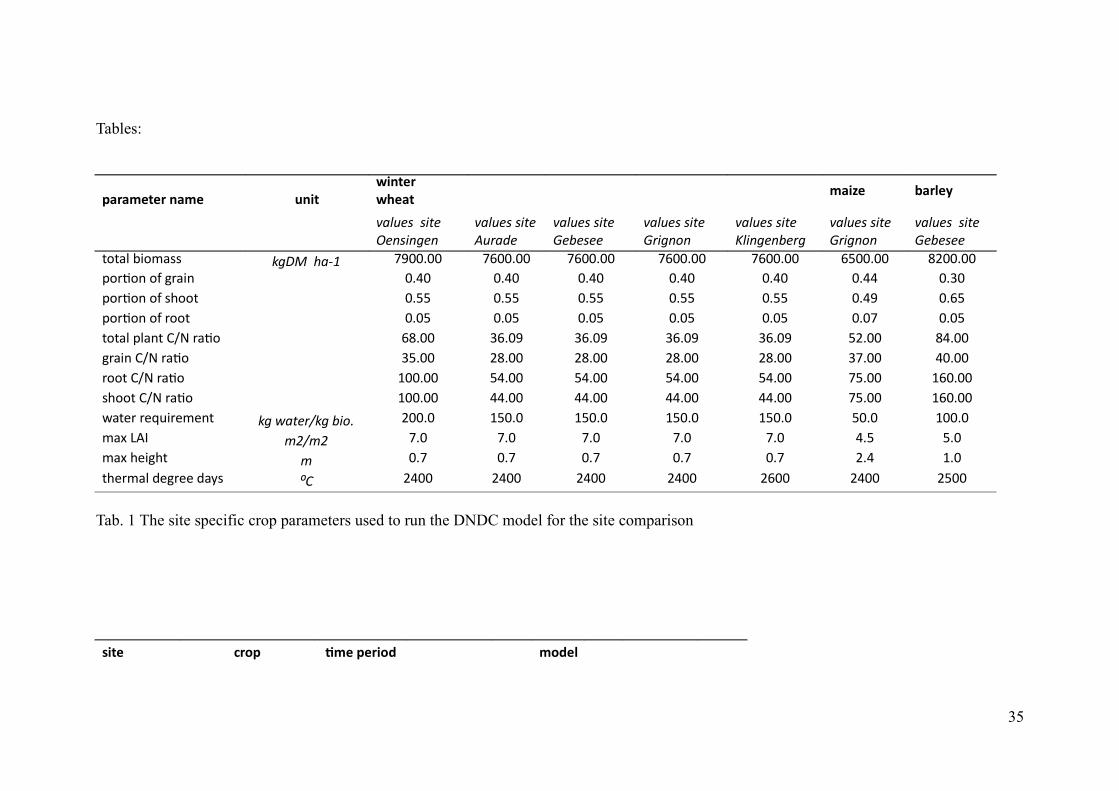
The four models were run at four sites (Oensingen, Grignon, Aurade, Klingenberg)

for one year of winter wheat (Triticum aestivum) at each site, one year for winter

barley (Hordeum vulgare) at Gebesee, and one year for maize (Zea mays) at Grignon.

However, the extent of our comparison is limited by model differences in the number

of crop types simulated and the kind of output data produced. For example, SPA has

no maize and ORCHIDEE-STICS no winter barley implementation yet, and CERES-

EGC produces no estimate of Reco. The combinations of sites, models, crops and years

are given in Table 2. Model results were compared accordingly.

A more detailed description of the sites is given in other papers in this special issue

(Kutsch et al. this issue, Ceschia et al. this issue).

2.2 Models

8

2.2.1 The DNDC model

The DNDC model (in this study version 9.2), is a general model of C and N

biogeochemistry in agricultural ecosystems {Li, 2005 #464; Li, 1994 #449; Li, 1992

#789}. It is a process-oriented simulation model, which contains four interacting sub-

models for soil climate, de-nitrification, decomposition and plant growth. The model

has been tested against numerous field data sets of nitrous oxide (N2O) emissions

{Tonitto, 2007 #788; Frolking, 1998 #790; David, 2009 #792; Abdalla #783} and soil

carbon dynamics {Smith, 1997 #452; Brown, 2002 #466; Li, 1997 #791; Zhang, 2006

#794}. In the application of DNDC presented here, we focus on analysing the

implementation of the carbon cycle in the decomposition and plant growth part of the

model, together with the section of the model to calculate the latent heat flux.

plant growth

DNDC simulates plant growth using an empirical approach calculating

photosynthesis, respiration, water and N demand, C allocation, crop yield, and litter

production on a daily time step for about sixty different crops. Photosynthesis is

calculated using the radiation use efficiency approach {Monteith, 1977 #294}, with

interception depending on leaf areas index based on Beer’s law. Phenology is

simulated using accumulative thermal degree days approach. A user defined amount

of litter either from roots or aboveground residue after harvest is assumed to enter the

carbon cycle of the model {Qiu, 2009 #793}.

soil carbon dynamics

9

The soil organic carbon (SOC) dynamics are simulated by assuming four main pools:

plant residue, microbial biomes, active humus, and passive humus. Each of the main

pools is subdivided into one or more sub-pools with different properties. The daily

decomposition rate is calculated depending on the relative size of each sub-pool and is

regulated by each pool size, its decomposition rate, the soil clay content, N

availability, soil temperature and moisture, and its depth in the soil profile. In the

process of the decomposition simulation, carbon is transferred to the soil pool with the

next lower decomposition rate, partially assimilated into microbial biomes, and

partially converted into CO2 {Qiu, 2009 #793}.

latent heat

Potential evapo-transpiration (ET) in DNDC is calculated using a daily average value

from the Thornthwaite formula {Thornthwaite, 1965 #503}. Subsequently, potential

ET is separated into potential evaporation and transpiration. To calculate the potential

transpiration, the water demand of plants is calculated based on the daily biomass

increment using the water/biomass ratio of the crops. The actual plant transpiration is

then calculated by taking the actual soil water content of the soil profile into account

{Li, 2006 #812}.

PLEASE INSERT TABLE 1

2.2.2 The ORCHIDEE-STICS model

ORCHIDEE-STICS is a coupled model {Gervois, 2008 #795; De Noblet-Ducoudré,

2004 #796} consisting of a dynamic global vegetation model ORCHIDEE {Krinner,

10

2005 #797}, and a process-oriented crop model STICS {Brisson, 2002 #798; Brisson,

1998 #799; Brisson, 2003 #800}.

The ORCHIDEE model calculates, for diverse vegetation types (plant functional

types), surface CO2, water vapour and heat fluxes driven by varying weather, and the

soil water and C pools dynamics. It contains a biophysical module, dealing with

photosynthesis and energy balance calculations each 30 min, and a carbon dynamics

module, dealing with phenology, growth, allocation, mortality and SOM

decomposition, on a daily time step.

For better representing cultivated plants, their phenology and management related

growth is calculated by the STICS model which is coupled to ORCHIDEE providing

daily foliar index, root density profiles, nitrogen stress, vegetation height, and

irrigation requirements. These variables are then sequentially assimilated into

ORCHIDEE each day to further calculate accurately gross primary production (GPP).

Currently, the ORCHIDEE-STICS model has been used for simulating Wheat,

Soybean and Maize although STICS has sufficiently generic parameterizations to

allow simulation of other crop species. The processes of the STICS sub model are:

plant growth

Crop growth is driven by the plant carbon accumulation {de Witt, 1978 #899}, solar

radiation intercepted by the foliage. According to the plant type, crop development is

driven either by a thermal index (degree-days), a photothermal index or a

photothermal index taking into account vernalisation. The vernalisation factor is the

ratio between the sum of vernalising days since planting and plant vernalisation

requirements {Weir, 1984 #900}. Water stress and nitrogen stress, if any, reduce leaf

growth and biomass accumulation, based on stress indices that are calculated in water

11

and nitrogen balance modules {Brisson, 2002 #798; Brisson, 1998 #799; Brisson,

2003 #800}.


latent heat flux

2.2.3 The SPA model

The Soil Plant Atmosphere model (SPA; {Williams, 1996 #802}) is a process-based

model that simulates ecosystem photosynthesis and water balance at fine temporal

and spatial scales (up to 30 minute time step, ten canopy and twenty soil layers). The

scale of parameterization (leaf-level) and prediction (canopy-level) have been

designed to allow the model to diagnose eddy flux data and to provide a tool for

scaling up leaf level processes to canopy and landscape scales {Williams, 2000

#803}.

plant growth

The SPA model employs the Farquhar approach of leaf-level photosynthesis

{Farquhar, 1980 #62} to calculate the amount of carbohydrates synthesised at each

time step. The carbohydrates are then allocated to one root and four aboveground

carbon pools (labile, foliage, stem and storage organ carbon pools), and accounts for

autotrophic and heterotrophic respiratory processes {Vertregt, 1987 #804}. The C

allocation pattern itself is dependent on the developmental stage (DS) of the crop

plant. DS is calculated as the sum of daily developmental rates, which are a function

12

of temperature, photoperiod, and vernalisation (Sus et al., this issue). Senescence is

calculated as a function of either mutual shading effects of canopies with a LAI > 4,

or developmental rate in the reproductive phase, whichever is dominant. Senescent

carbon is either remobilised and subsequently reallocated to the growing storage

organ, or added to a standing dead leaf biomass carbon pool.


At harvest, the fraction of the aboveground biomass exported from the field is

estimated by the storage organ C content plus non-crop residue leaf and stem C mass.

The residual crop biomass gradually enters the litter carbon pool. The fraction of crop

residue entering either the litter or soil carbon pool further depends on land

management and can be adjusted accordingly. Following this approach, SPA models

the carbon mass balance for winter/spring barley and wheat (Sus et al. this issue)

latent heat

SPA uses the Penman-Monteith equation to determine leaf-level transpiration

{Penman, 1948 #497; Monteith, 1965 #396; Monteith, 1977 #294}. It is linked to the

photosynthesis module by a novel model of stomatal conductance that optimizes daily

carbon gain per unit leaf nitrogen, within the limitations of canopy water storage and

soil to canopy water transport.

2.2.4 The CERES-EGC model

The original CERES model is a soil-crop model {Jones, 1986 #814}. It was extended

to be CERES-EGC by {Gabrielle, 2006 #813; Lehuger, 2009 #860} by moving the

13

focus towards the simulation of nitrogen cycle related processes such as nitrate

leaching, emissions of N2O and nitrogen oxides. CERES-EGC runs on a daily time

step, and requires daily rain, mean air temperature and Penman potential evapo-

transpiration {Penman, 1948 #497} as forcing variables to calculate actual evapo-

transpiration.

CERES-EGC simulates water, carbon and nitrogen in the soil-crop systems in a

number of sub modules. A physical sub-model simulates heat, water and nitrate

movement in the soil. It is also responsible for the calculation of soil evaporation,

plant water uptake and transpiration. A biological sub-model simulates the growth and

phenology of the crops.

plant growth

The model calculates net photosynthesis as a linear function of intercepted radiation

according to the Monteith approach {Monteith, 1977 #294}, with light interception

depending on leaf area index based on Beer’s law. The key species specific parameter

in this calculation is the radiation use efficiency (RUE) defined as the dry biomass

produced per unit of radiation intercepted. Photosynthates are partitioned on a daily

basis to currently growing organs (roots, leaves, stems, fruits) according to crop

development stage. The latter is driven by the accumulation of growing degree days,

as well as cold temperature and day-length for crops sensitive to vernalisation and

photoperiod. Lastly, crop N uptake is computed through a supply/demand scheme,

with soil supply depending on soil nitrate and ammonium concentrations and root

length density.

14

soil carbon

A micro-biological sub-model simulates the turnover of organic matter in the plough

layer. Decomposition, mineralisation and N-immobilisation are modelled with three

pools of organic matter (OM): the labile OM, the microbial biomass and the humads.

Kinetic rate constants de ne the C and N ows between the different pools. Directfi fl

eld emissions of COfi 2, N2O, NO and NH3 into the atmosphere are simulated with

different trace gas modules (Lehuger et al. this issue).

latent heat

The Penman potential evapo-transpiration {Penman, 1948 #497} as forcing variables

to calculate actual evapo-transpiration based on the water status of the soil and crop

respectively.

2.2.5 Simulation set-up

Input data

Models are driven by meteorological variables derived from half hourly

measurements at each site. Simulation time steps differ also among models (and

consequently time resolution of input meteorological variables): from daily (for

DNDC) and CERES-EGC) to half-hourly (for SPA and ORCHIDEE-STICS). The

number of meteorological variables used also differs among the models: from only

two for DNDC (temperature and precipitation) to up to six for ORCHIDEE-STICS

(temperature, precipitation, incident long and short-wave radiation, relative humidity

and wind speed).

15

In case of gaps in the on-site daily time series the data from the nearest climate station

out of the ECAD dataset was used to gap-fill with daily values for models with daily

time steps {Klein Tank, 2002 #801}. In case of gaps in the half hourly data reuired by

the ORCHIDEE-STICS and SPA, data were gap filled with long term site specific

half hourly average.

The soil texture is determined from measurements made on each site (Kutsch et al.

this issue, Sus et al., this issue) and prescribed accordingly for all four models.

Management events, such as fertilisation, irrigation, planting, harvest or ploughing are

also defined by on-site observed values (Kutsch et al. this issue). In the SPA model,

the effects of fertilization are not taken into account, but reported harvest dates and

crop residue management are considered in the model runs.

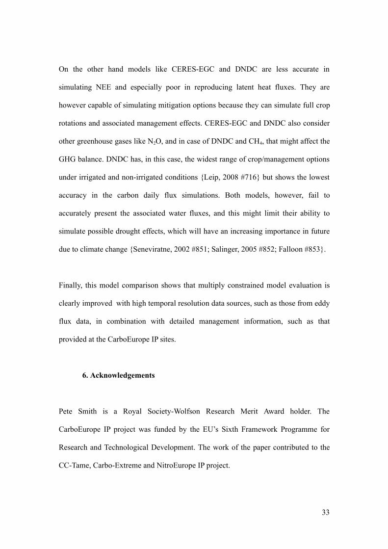
The three simulated crops, winter wheat (Triticum aestivum L.), Winter Barley winter

barley (Hordeum vulgare) and maize (Zea mays L.), were parameterised for each

model using ‘standard’ published values {Mueller, 2005 #539; Kätterer, 1997 #765;

Van Den Boogaard, 1997 #767; McMaster, 2003 #774 ; Lohila, 2003 #641; Juskiw,

2001 #645; López, 1997 #775} or data provided by the site. For the DNDC model,

values given in table 1 are for the time of harvest as prescribed in the DNDC user

manual. For the estimation of plant C/N ratios in DNDC, site data for biomass and

carbon and nitrogen content were used. Where carbon and nitrogen content data were

not available, fertiliser application data, provided by the site managers, were used to

derive site specific C/N ratios under the assumption of optimum nitrogen supply

during growth.

16

Initialisation procedure

For the initialisation of the soil carbon and nitrogen pools, the DNDC model was run

for ten years using daily ECAD weather data from the nearest weather station {Klein

Tank, 2002 #801}. The litter input for the initialisation period was manually adjusted

so that modelled matched measured total soil organic carbon at the beginning of the

simulation period. The fertilizer input for this initialisation period was assumed to be

in the same order of magnitude as the mineral fertilizer input during the simulation

period. For simulations performed by ORCHIDEE-STICS, the soil carbon pools were

initialized to their steady state equilibrium values after a thousand-years spin-up

during which climate and management practice of the simulated year were repeatedly

cycled. For SPA simulations, the initial soil organic matter as well as labile carbon

contents are estimated, based on field observations reported in the literature {Anthoni,

2004 #807; Aubinet, 2008 #808; Halley, 1988 #805}. The initial labile carbon content

is equal to the seed carbon content at sowing. The CERES-EGC model was run for

two rotations in all sites before the measurement period to stabilize the C and N soil

pools and dampen the initial conditions. The same meteorological data were

repeatedly used in case the historical data were not available.

DNDC was set up to run for the full crop rotation using litter inputs based on the

calculated crop growth. The optimum yield parameter was adjusted to match the site

specific yields. The DNDC model does not incorporate the concept of crop

germination and emergence, it assumes an initial biomass at the day of sowing with

the immediate start of photosynthesis. In order to simulate a realistic crop growth we

assume 20 days for the crop to emerge from the day of seeding to the start of

photosynthesis {McMaster, 2003 #774; Stone, 1999 #770}. For the ORCHIDEE-

17

STICS runs, one simulation was performed for each crop season. The SPA runs have

been initiated at sowing (date as reported from the site) and terminated by the end of

the following year. It is important to note that the SPA outputs are only truly

representative of the actual growth period from sowing to harvest, as no post-harvest

voluntary re-growth, ploughing or sowing has been considered. However, reported

fractions of crop residual biomass were considered for the simulation of post-harvest

heterotrophic respiration fluxes (Sus et al. this issue). The simulations of CERES-

EGC were set up for full crop rotations. The sowing date of each crop was initiated in

the management file and harvest time was simulated when crops attained the

physiological maturity. Grain and straw were exported out of the field while crop

residues and roots were incorporated into the SOM pools at the date of the post-

harvest tillage. Catch crops (at Grignon) and volunteers from the previous crop (at

Auradé) were simulated between the crop seasons of a winter crop (barley and wheat)

and a spring crop (maize and sunflower).


Model comparison

We use the site eddy covariance derived data for GPP, NEE, Reco {Reichstein, 2005

#827} and latent heat aggregated on a daily time step for the model comparison. The

data are provided in gap filled format which is checked for errors and outliers and

aggregated for different time intervals from half hourly to weekly in the CarboEurope

IP ecosystem database {Papale, 2006 #824; Papale, 2006 #825; Moffat, 2007 #815;

Reichstein, 2005 #816}.

18

The statistical methods of the model comparison are based on {Smith, 1997 #784;

Morales, 2005 #531}. The data analysis itself was performed by the statistical

package R {R, 2009 #809}. To determine if the daily measured NEE, GPP and Reco

data are normally distributed we used the Shapiro-Wilk implementation in R

{Royston, 1992 #835} independently for each site and each year of the comparison.

The highly significant result of the test (p<0.01) indicates a very high probability that

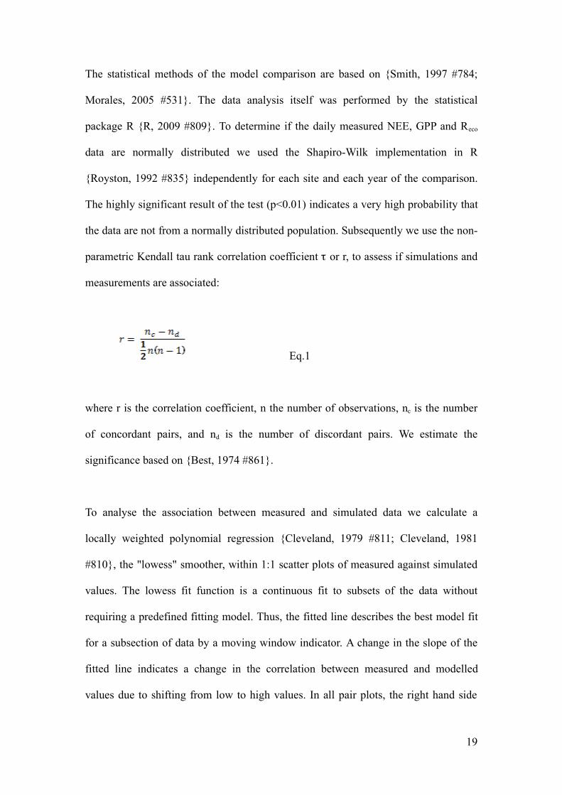
the data are not from a normally distributed population. Subsequently we use the non-

parametric Kendall tau rank correlation coefficient or r, to assess if simulations and$

measurements are associated:

Eq.1

where r is the correlation coefficient, n the number of observations, nc is the number

of concordant pairs, and nd is the number of discordant pairs. We estimate the

significance based on {Best, 1974 #861}.

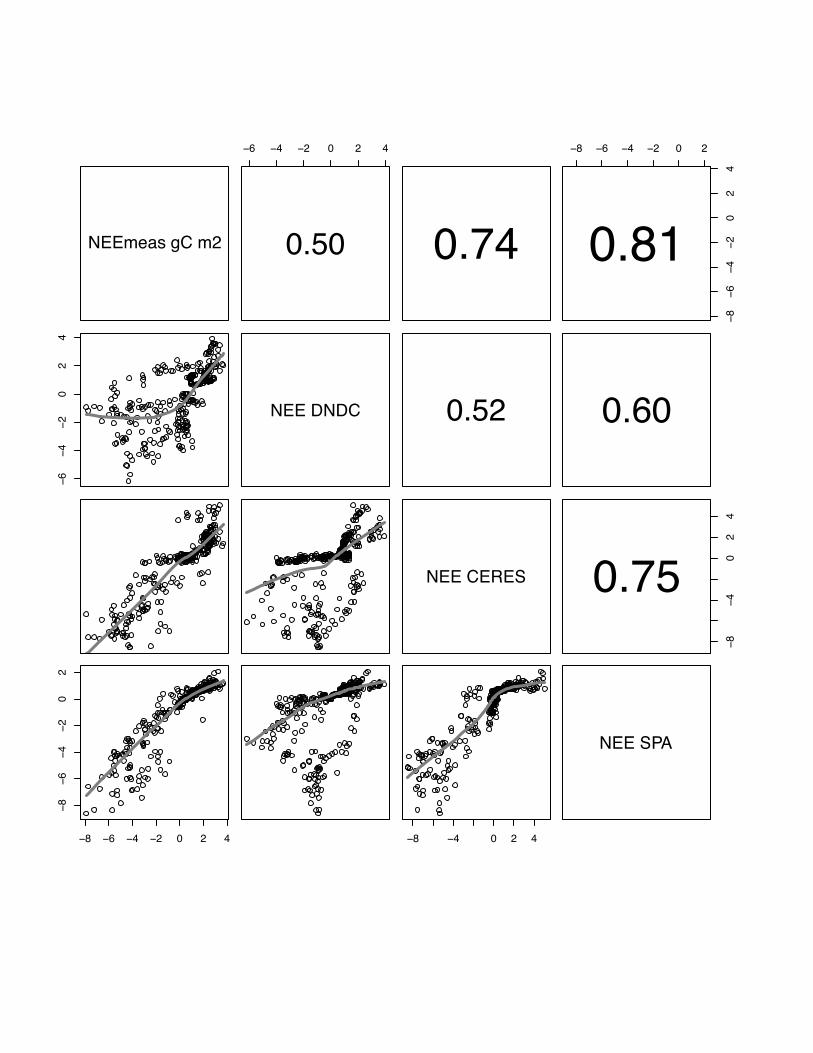
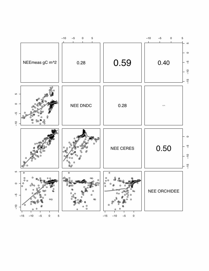
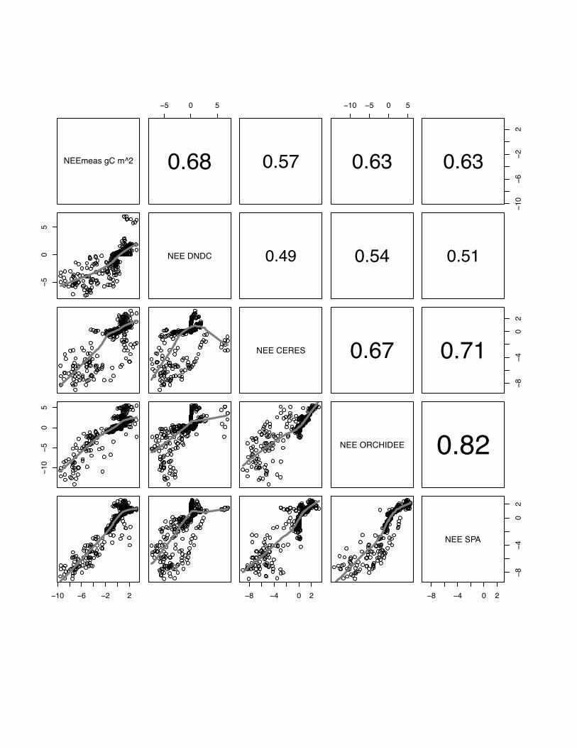
To analyse the association between measured and simulated data we calculate a

locally weighted polynomial regression {Cleveland, 1979 #811; Cleveland, 1981

#810}, the "lowess" smoother, within 1:1 scatter plots of measured against simulated

values. The lowess fit function is a continuous fit to subsets of the data without

requiring a predefined fitting model. Thus, the fitted line describes the best model fit

for a subsection of data by a moving window indicator. A change in the slope of the

fitted line indicates a change in the correlation between measured and modelled

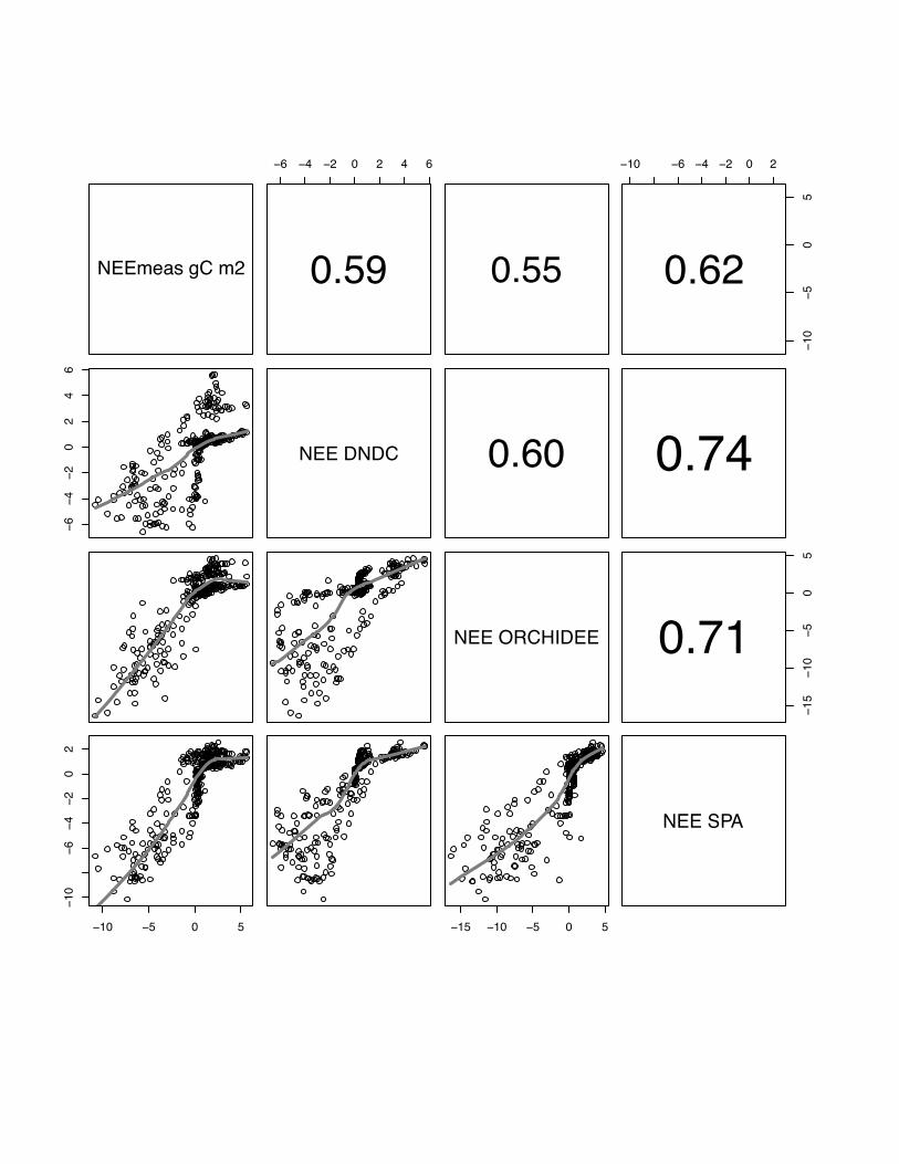
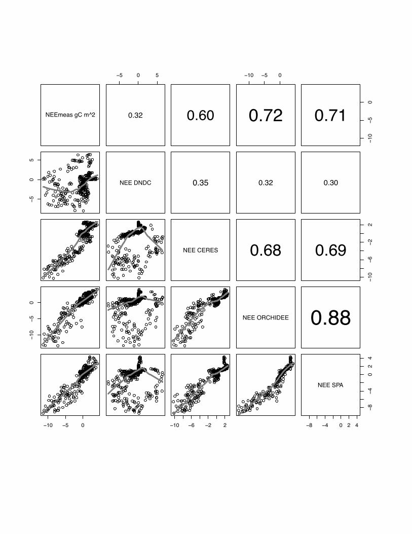
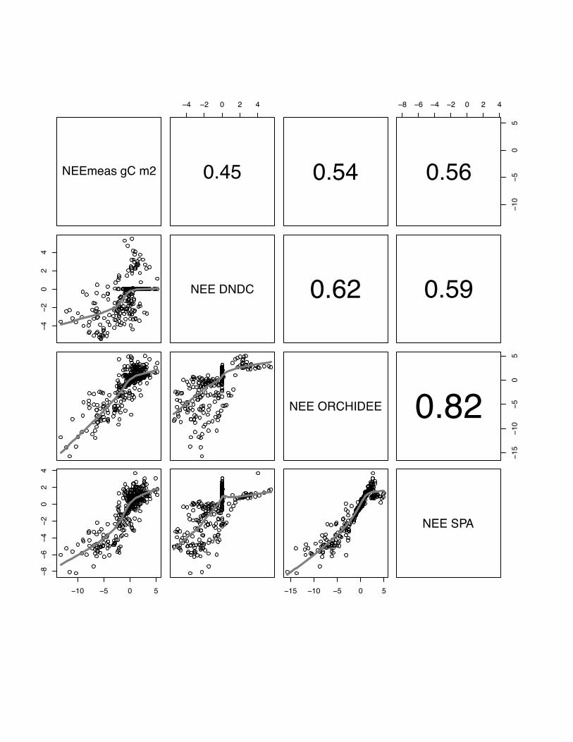
values due to shifting from low to high values. In all pair plots, the right hand side

19

panel shows the r values in black for significant correlation coefficient results

(p<0.05), and in light grey for non-significant associations (p>0.05). The size of the

text indicates the strength of the association. We use a 95% confidence interval as

suggested by {Smith, 1997 #784: Morales, 2005 #531}.

The model efficiency factor E {Nash, 1979 #298} is another measure of model

performance. It compares the squared sum of the absolute error with the squared sum

of the difference between the observations and their mean value. It compares the

ability of the model to reproduce the daily data variability with a much simpler model

that is based on the arithmetic mean of the measurements:

Eq. 2

where Oi are the observed values, Pi are the simulated values, n are the total number

of observations and i the current observation. It ranges from 1 to - . Any model!

giving a negative value cannot be recommended, a value of 0 indicates that the model

does not perform better than using the mean of the observations, and values close to 1

indicate a ‘near-perfect’ fit.

To compare the annual carbon balance of the sites, the total annual flux is calculated

for observed and simulated NEE:

Eq. 3

20

Eq 4

where mo,i is the cumulative sum of the daily (i) observed fluxes and mp,i the

cumulative sum of the simulated flux. The difference of the two is the absolute error

x presented in table 3. We tested the median of the two cumulative flux distributions#

for significant differences on the 95% confidence level by using the R implementation

of the Wilcoxon rank sum test {Corder, 2009 #854; Hollander, 1973 #855}.

2. Results

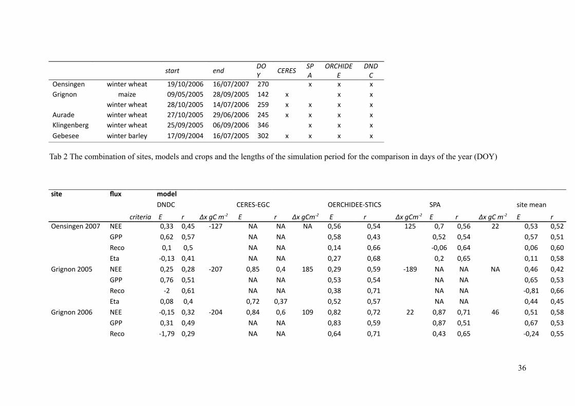
The statistical results of r and E for all sites are summarised in table 3 and in the

figures that show the site to site performance in terms of r. There are common patterns

for all sites and for all models which are:

o inconsistency between the models to reproduce low carbon fluxes ranging

between -2 gC m2 day-1 and 2 g C m2 day-1 (odd numbered figures 1-11).

o all models have problems with capturing the crop phenology, which is indirectly

indicated by either an overestimation of the amplitude of growth in the later

stage of crop development (mainly the case for ORCHIDEE-STICS, SPA and

CERES model) or a phase shift of growth as seen for DNDC (especially for

winter wheat and barley, by simulating a too early onset of growth) (even

numbered figures 2-12)

o a good to very-good fit for GPP and Reco at fluxes below respectively above the

-2 gC m2 day-1 and 2 g C m2 day-1 flux rates, but a relatively poorer fit for NEE.

21

o DNDC and CERES-EGC: a relatively poor performance in reproducing the

latent heat flux in contrast to a better performance for NEE, GPP and Reco,

suggesting problems in the coupling of the water and carbon flux in these

models.


3.1 NEE

There is a wide range in the performance of the various models to reproduce the

measured NEE patterns at different sites and in different years, and also between

models at one site in the same year. Correlations range from r=0.28, p<0.05 for

DNDC simulating maize in year 2005 at Grignon to r=0.81, p<0.05 for the SPA model

simulating winter barley at Gebesee in 2007 (see table 3). In general, all models

perform better for simulating winter crops (site mean: E=56, r=0.61) than the summer

maize crop at Grignon (site mean: E=0.46, r=0.42).

In general, there is a better inter-model agreement between CERES-EGC,

ORCHIDEE-STICS and SPA than between any of these models and DNDC. The only

exception is the Klingenberg site where we observe a slightly better agreement

between SPA and DNDC than between ORCHIDEE-STICS and DNDC. If we test

average correlation of all models per site, models perform on average best at Gebesee

with winter barley in 2007 (r=0.68), followed by Aurade (r=0.65), Klingenberg

(r=0.61), Girgnon 2006 (r=0.58), Oensingen (r=0.52) and maize crop in Grignon in

2005 (r=0.42). Even though these results are relatively satisfying, all models expose a

22

weak and inconsistent performance at all sites for low fluxes in the range of -2 gC m2

day-1 to 2 g C m2 day-1 .

If we compare cumulative NEE fluxes (even-numbered fig. 2-12), we observe a

mismatch for all models in the early stage of the growing season, when low fluxes are

predominate. The DNDC model shows a stronger divergence from measurements

compared to the other models in the first 100 days of the year (DOY). The

ORCHIDEE-STICS, SPA and CERES-ECG models start with very similar trajectories

but begin to diverge between DOY 100 and 200 at most of the sites, except for maize

at Grignon in 2005. A common pattern for the three models is to overestimate the

NEE peak and the failure to reproduce the senescence and post harvest fluxes. This

leads to a mismatch of the cumulative NEE for the year. In general, the SPA model

shows the best performance in terms of NEE for the sites even though deficiencies

remain in reproducing peak and post-harvest NEE fluxes.

PLEASE INSERT FIG. 1 to 12

3.3 Reco

The ranking the models according to their association with the data shows

ORCHIDEE-STICS with the best performance on average over all sites (model mean:

r=0.72, p<0.05). This model is also consistent in its performance over all sites with

comparable r values (table 3). Between models the r values vary strongly from r=0.38

for DNDC in Aurade to r=0.79 (p<0.05) for ORCHIDEE-STICS at Klingenberg in

2006. Similar as for the simulation of NEE, we can identify the highest significant

agreement between SPA and ORCHIDEE-STICS (Note: CERES-EGC does not

23

simulate Reco), and a lower association between these two models and DNDC.

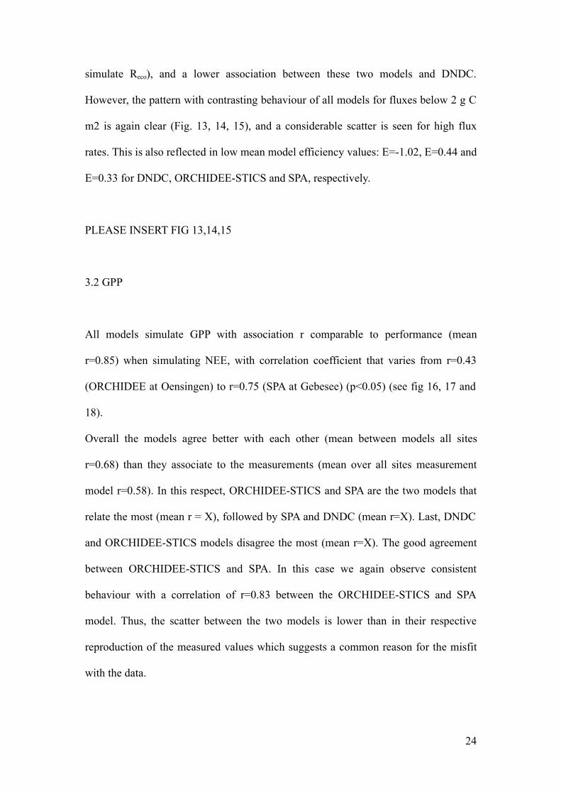
However, the pattern with contrasting behaviour of all models for fluxes below 2 g C

m2 is again clear (Fig. 13, 14, 15), and a considerable scatter is seen for high flux

rates. This is also reflected in low mean model efficiency values: E=-1.02, E=0.44 and

E=0.33 for DNDC, ORCHIDEE-STICS and SPA, respectively.

PLEASE INSERT FIG 13,14,15

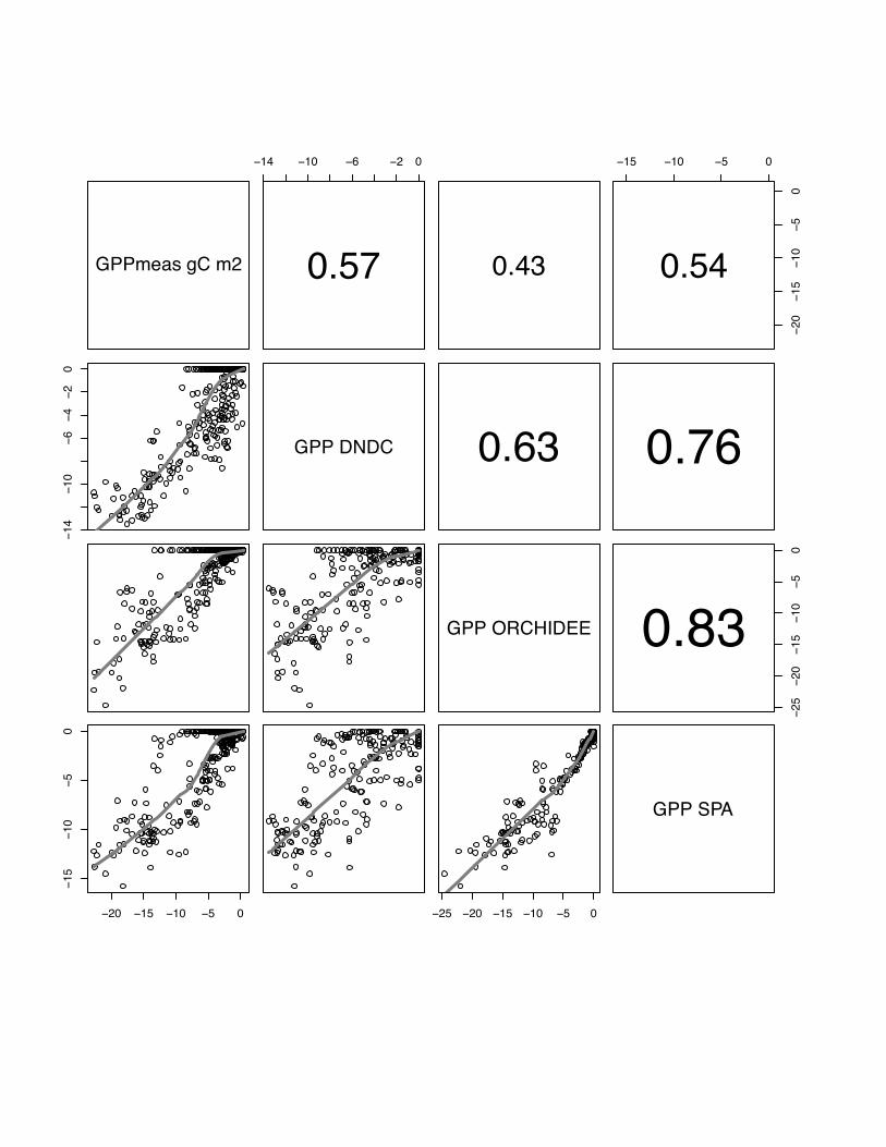
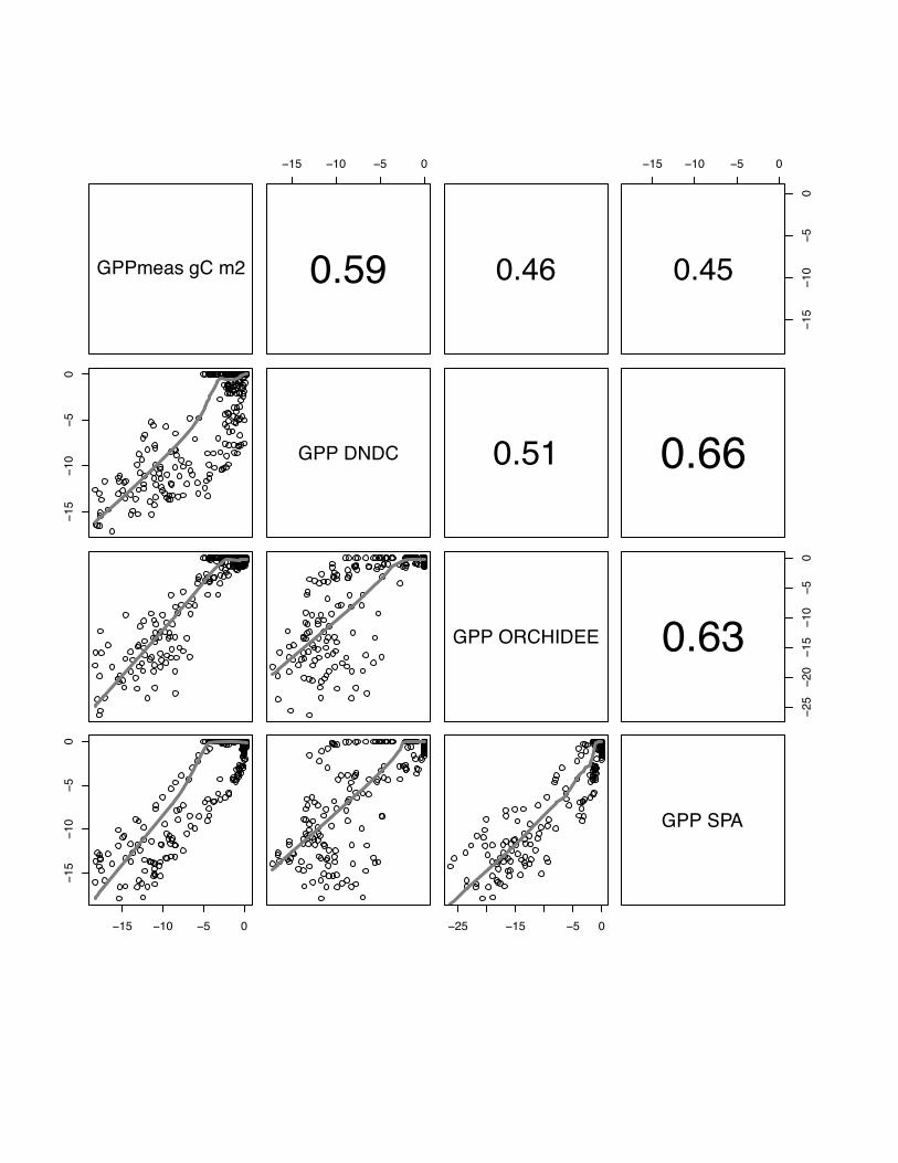
3.2 GPP

All models simulate GPP with association r comparable to performance (mean

r=0.85) when simulating NEE, with correlation coefficient that varies from r=0.43

(ORCHIDEE at Oensingen) to r=0.75 (SPA at Gebesee) (p<0.05) (see fig 16, 17 and

18).

Overall the models agree better with each other (mean between models all sites

r=0.68) than they associate to the measurements (mean over all sites measurement

model r=0.58). In this respect, ORCHIDEE-STICS and SPA are the two models that

relate the most (mean r = X), followed by SPA and DNDC (mean r=X). Last, DNDC

and ORCHIDEE-STICS models disagree the most (mean r=X). The good agreement

between ORCHIDEE-STICS and SPA. In this case we again observe consistent

behaviour with a correlation of r=0.83 between the ORCHIDEE-STICS and SPA

model. Thus, the scatter between the two models is lower than in their respective

reproduction of the measured values which suggests a common reason for the misfit

with the data.

24

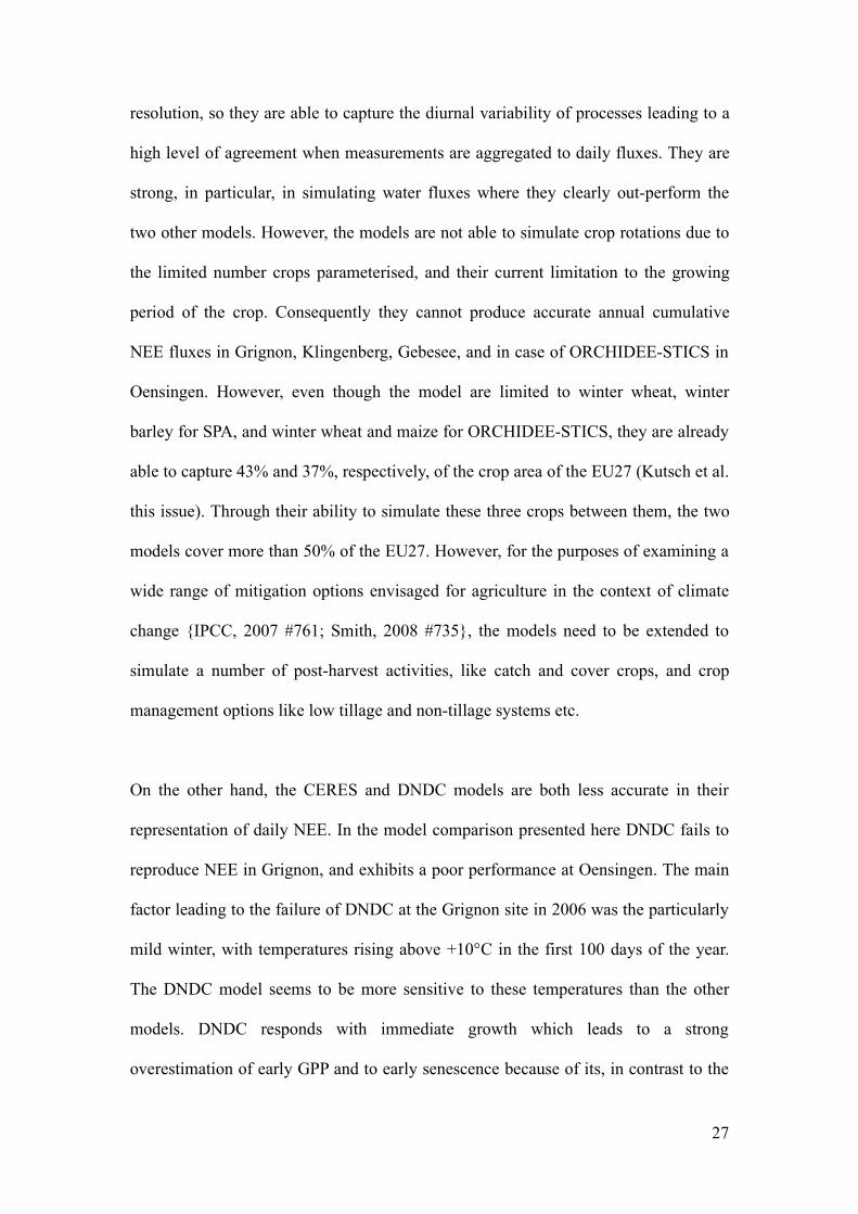
Model-data comparisons exhibit a strong mismatch for low fluxes as indicated by a

similar and almost ‘flat’ shape of the regression line for the comparison with low

measured values (see Fig. 16-18). As already observed r score, there is a better

agreement for these low fluxes between ORCHIDEE-STICS and SPA than between

each of the two models and the measurements.

Overall model-data agreement as evaluated by the Nash-Sutcliffe E is relatively high,

being generally greater than 0.55. It is minimal for DNDC at Grignon in 2006

(E=0.31) and goes up to 0.80 for three model-site combinations (ORCHIDEE-SITCS

and SPA at Grignon 2006 and SPA at Gebesee).

PLEASE INSERT FIG 16, 17, 18

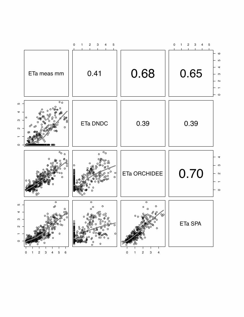
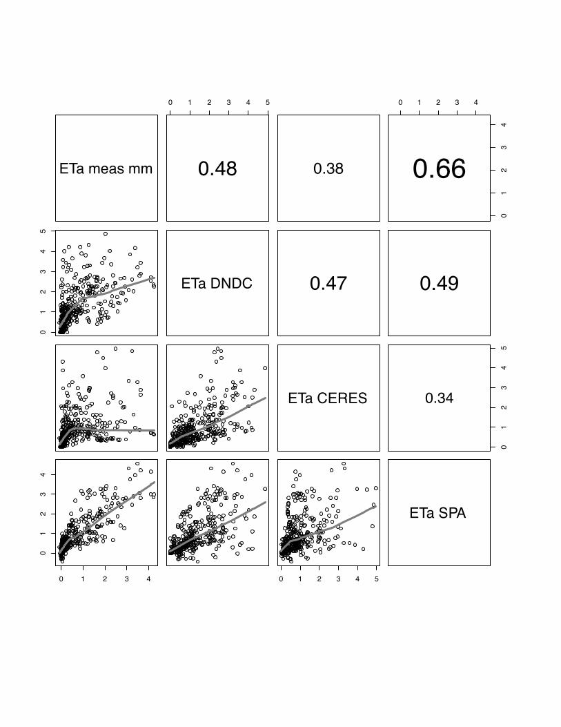
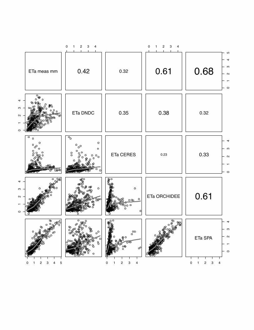
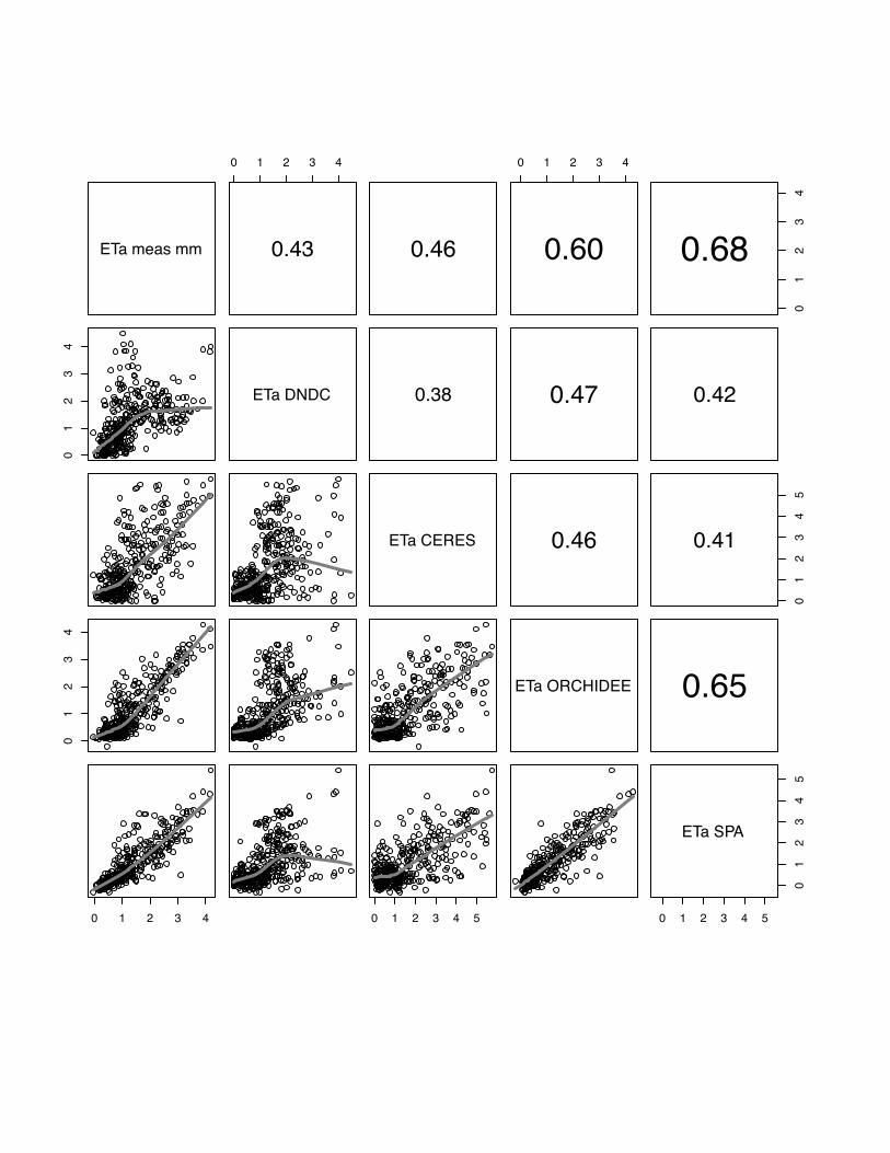
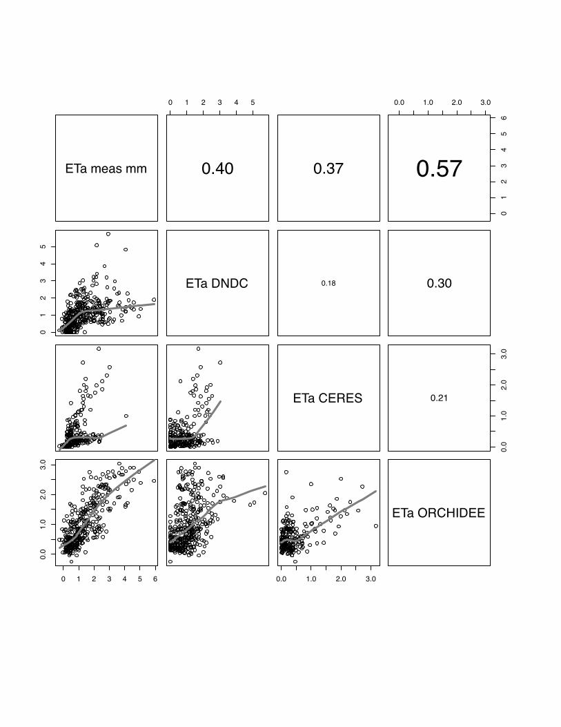
3.4 ETa

The comparison of observed and modelled evapotranspiration fluxes generally shows

that ORCHIDEE-STICS and SPA show highest correlations with measurements

(mean r for all sites: 0.60 for ORCHIDEE-STICS, 0.69 for SPA). Again, these models

also exhibit a considerable degree of cross-correlation, indicating a general agreement

in the response to driving variables. In relation to that, the accuracy of modelled ETa

as simulated by CERES-EGC (mean r: 0.38) and DNDC (mean r: 0.45) is

considerably lower. For CERES-EGC and DNDC, the relationship between modelled

and observed ETa, expressed by the slope of the lowess fit curve, is changing around

a value of 1 mm d-1. Beyond this value, the fit curve gradually takes over a quasi-

logarithmic behaviour for most scatter plots. For certain sites (e.g. both Grignon

25

years), DNDC and CERES-EGC fail to reproduce high flux rates, indicated by a high

degree of scattering around the fit curve. The correlation of modelled values is high

between DNDC and CERE-EGC, and even higher than with the observations for the

Gebesee site.

We found considerably low values of model efficiency for DNDC and CERES-EGC,

which are negative for Grignon 2006, Gebesee and Klingenberg. For SPA and

ORCHIDEE-STICS, E ranges from 0.2 (SPA at Oensingen) to 0.78 (ORCHIDEE-

STICS at Grignon 2006). Thus, the overall efficiency of these two models is higher

and broadly satisfying.

In general, lower evapotranspiration fluxes were captured with higher accuracy by all

models, which is indicated by an increasing data spread beyond 1 mm d-1 in most of

the scattering plots (fig 19-23).

PLEASE INSERT FIG 19 to 23

4. Discussion

The aim of the paper was to test four models for accuracy in simulating the main

components of the carbon cycle, net ecosystem exchange (NEE), ecosystem

respiration (Reco) and gross primary production (GPP) in connection with the actual

evapo-transpiration (ETa) on a daily time scale over a gradient of environmental

conditions in Europe. The results show a heterogeneous picture, with strong

differences between models and between sites. The two models with the highest

accuracy over all sites when simulating daily NEE and latent heat are SPA and

ORCHIDEE-STICS. Both models run on a half hourly time-step with a high process

26

resolution, so they are able to capture the diurnal variability of processes leading to a

high level of agreement when measurements are aggregated to daily fluxes. They are

strong, in particular, in simulating water fluxes where they clearly out-perform the

two other models. However, the models are not able to simulate crop rotations due to

the limited number crops parameterised, and their current limitation to the growing

period of the crop. Consequently they cannot produce accurate annual cumulative

NEE fluxes in Grignon, Klingenberg, Gebesee, and in case of ORCHIDEE-STICS in

Oensingen. However, even though the model are limited to winter wheat, winter

barley for SPA, and winter wheat and maize for ORCHIDEE-STICS, they are already

able to capture 43% and 37%, respectively, of the crop area of the EU27 (Kutsch et al.

this issue). Through their ability to simulate these three crops between them, the two

models cover more than 50% of the EU27. However, for the purposes of examining a

wide range of mitigation options envisaged for agriculture in the context of climate

change {IPCC, 2007 #761; Smith, 2008 #735}, the models need to be extended to

simulate a number of post-harvest activities, like catch and cover crops, and crop

management options like low tillage and non-tillage systems etc.

On the other hand, the CERES and DNDC models are both less accurate in their

representation of daily NEE. In the model comparison presented here DNDC fails to

reproduce NEE in Grignon, and exhibits a poor performance at Oensingen. The main

factor leading to the failure of DNDC at the Grignon site in 2006 was the particularly

mild winter, with temperatures rising above +10°C in the first 100 days of the year.

The DNDC model seems to be more sensitive to these temperatures than the other

models. DNDC responds with immediate growth which leads to a strong

overestimation of early GPP and to early senescence because of its, in contrast to the

27

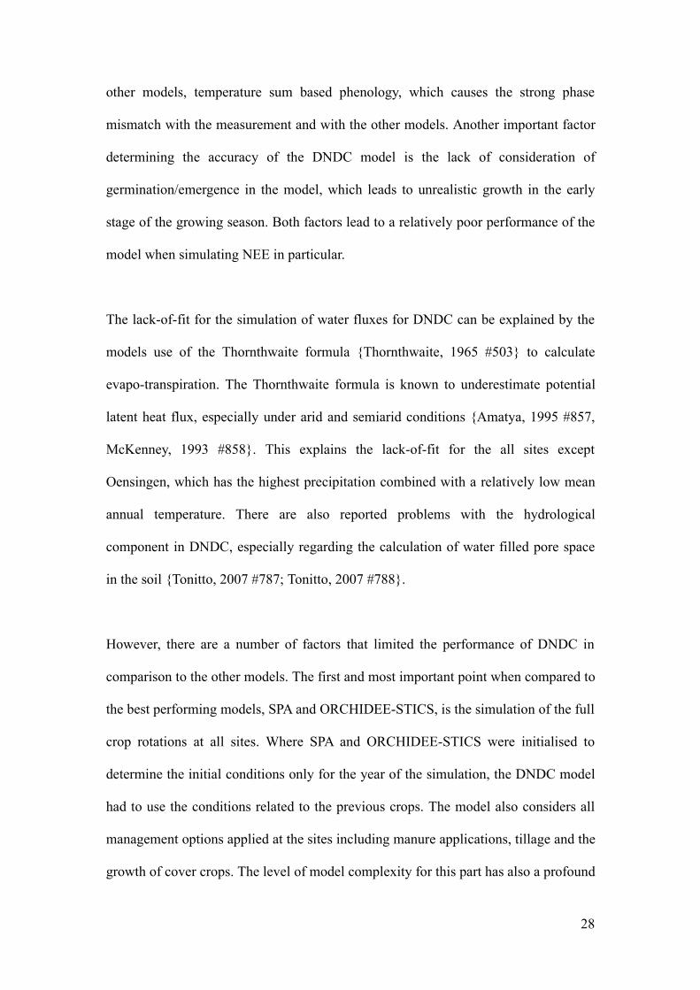
other models, temperature sum based phenology, which causes the strong phase

mismatch with the measurement and with the other models. Another important factor

determining the accuracy of the DNDC model is the lack of consideration of

germination/emergence in the model, which leads to unrealistic growth in the early

stage of the growing season. Both factors lead to a relatively poor performance of the

model when simulating NEE in particular.

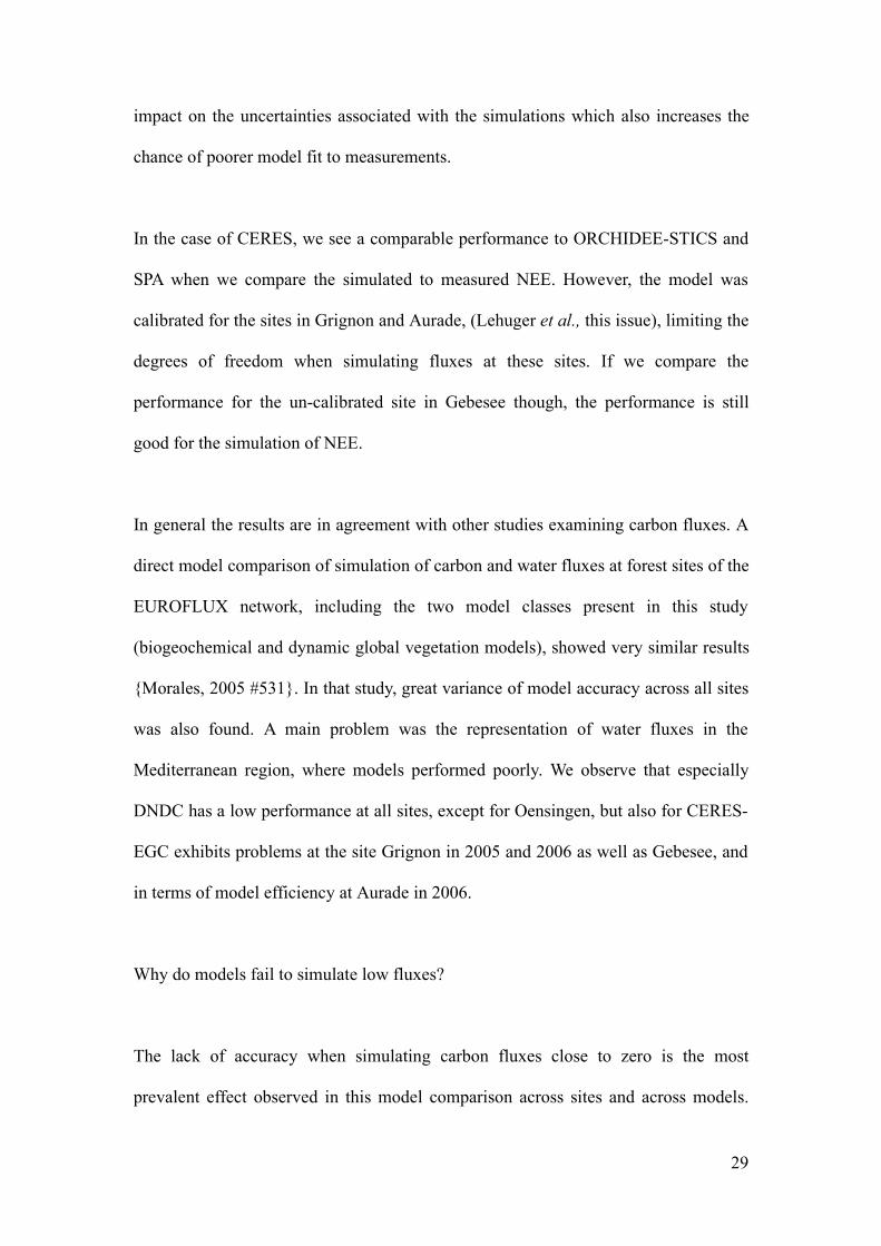
The lack-of-fit for the simulation of water fluxes for DNDC can be explained by the

models use of the Thornthwaite formula {Thornthwaite, 1965 #503} to calculate

evapo-transpiration. The Thornthwaite formula is known to underestimate potential

latent heat flux, especially under arid and semiarid conditions {Amatya, 1995 #857,

McKenney, 1993 #858}. This explains the lack-of-fit for the all sites except

Oensingen, which has the highest precipitation combined with a relatively low mean

annual temperature. There are also reported problems with the hydrological

component in DNDC, especially regarding the calculation of water filled pore space

in the soil {Tonitto, 2007 #787; Tonitto, 2007 #788}.

However, there are a number of factors that limited the performance of DNDC in

comparison to the other models. The first and most important point when compared to

the best performing models, SPA and ORCHIDEE-STICS, is the simulation of the full

crop rotations at all sites. Where SPA and ORCHIDEE-STICS were initialised to

determine the initial conditions only for the year of the simulation, the DNDC model

had to use the conditions related to the previous crops. The model also considers all

management options applied at the sites including manure applications, tillage and the

growth of cover crops. The level of model complexity for this part has also a profound

28

impact on the uncertainties associated with the simulations which also increases the

chance of poorer model fit to measurements.

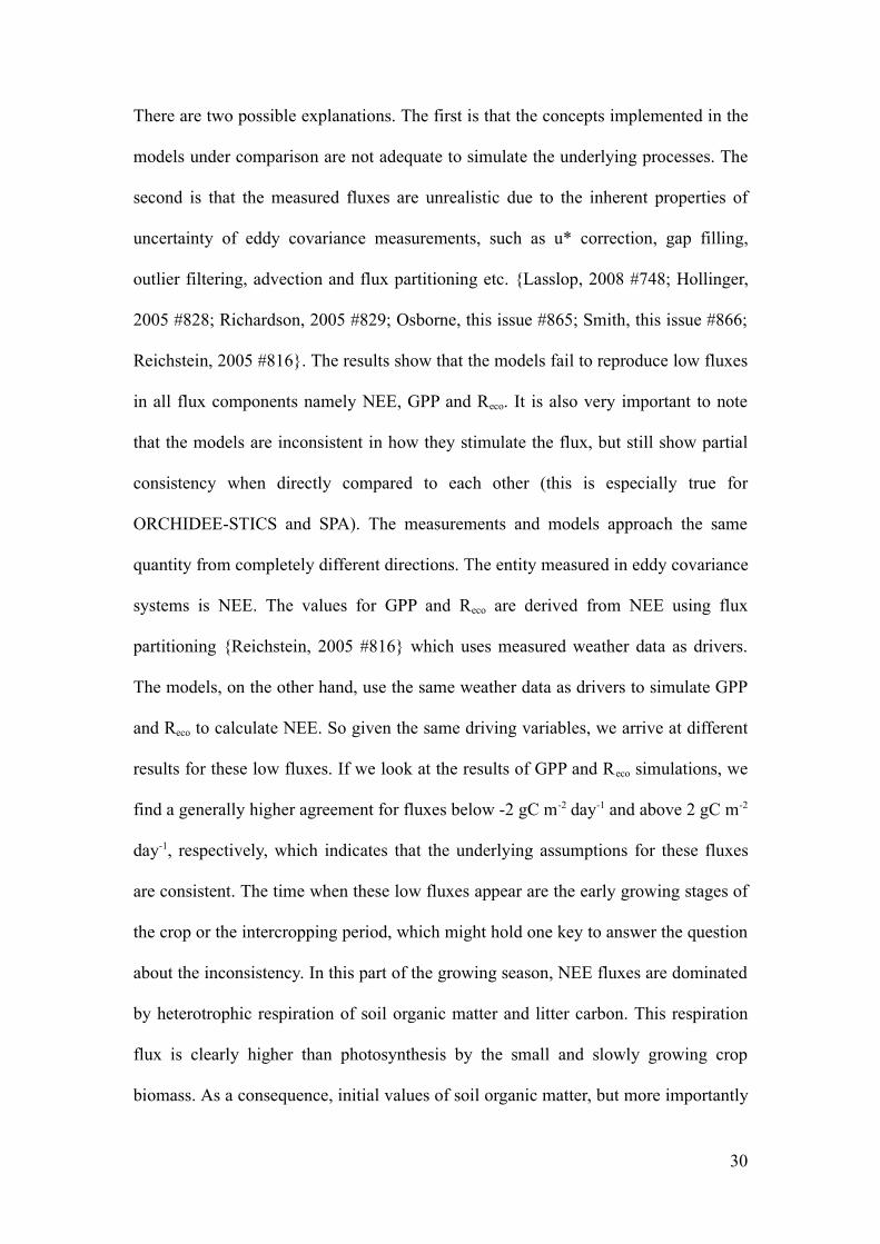
In the case of CERES, we see a comparable performance to ORCHIDEE-STICS and

SPA when we compare the simulated to measured NEE. However, the model was

calibrated for the sites in Grignon and Aurade, (Lehuger et al., this issue), limiting the

degrees of freedom when simulating fluxes at these sites. If we compare the

performance for the un-calibrated site in Gebesee though, the performance is still

good for the simulation of NEE.

In general the results are in agreement with other studies examining carbon fluxes. A

direct model comparison of simulation of carbon and water fluxes at forest sites of the

EUROFLUX network, including the two model classes present in this study

(biogeochemical and dynamic global vegetation models), showed very similar results

{Morales, 2005 #531}. In that study, great variance of model accuracy across all sites

was also found. A main problem was the representation of water fluxes in the

Mediterranean region, where models performed poorly. We observe that especially

DNDC has a low performance at all sites, except for Oensingen, but also for CERES-

EGC exhibits problems at the site Grignon in 2005 and 2006 as well as Gebesee, and

in terms of model efficiency at Aurade in 2006.

Why do models fail to simulate low fluxes?

The lack of accuracy when simulating carbon fluxes close to zero is the most

prevalent effect observed in this model comparison across sites and across models.

29

There are two possible explanations. The first is that the concepts implemented in the

models under comparison are not adequate to simulate the underlying processes. The

second is that the measured fluxes are unrealistic due to the inherent properties of

uncertainty of eddy covariance measurements, such as u* correction, gap filling,

outlier filtering, advection and flux partitioning etc. {Lasslop, 2008 #748; Hollinger,

2005 #828; Richardson, 2005 #829; Osborne, this issue #865; Smith, this issue #866;

Reichstein, 2005 #816}. The results show that the models fail to reproduce low fluxes

in all flux components namely NEE, GPP and Reco. It is also very important to note

that the models are inconsistent in how they stimulate the flux, but still show partial

consistency when directly compared to each other (this is especially true for

ORCHIDEE-STICS and SPA). The measurements and models approach the same

quantity from completely different directions. The entity measured in eddy covariance

systems is NEE. The values for GPP and Reco are derived from NEE using flux

partitioning {Reichstein, 2005 #816} which uses measured weather data as drivers.

The models, on the other hand, use the same weather data as drivers to simulate GPP

and Reco to calculate NEE. So given the same driving variables, we arrive at different

results for these low fluxes. If we look at the results of GPP and Reco simulations, we

find a generally higher agreement for fluxes below -2 gC m-2 day-1 and above 2 gC m-2

day-1, respectively, which indicates that the underlying assumptions for these fluxes

are consistent. The time when these low fluxes appear are the early growing stages of

the crop or the intercropping period, which might hold one key to answer the question

about the inconsistency. In this part of the growing season, NEE fluxes are dominated

by heterotrophic respiration of soil organic matter and litter carbon. This respiration

flux is clearly higher than photosynthesis by the small and slowly growing crop

biomass. As a consequence, initial values of soil organic matter, but more importantly

30

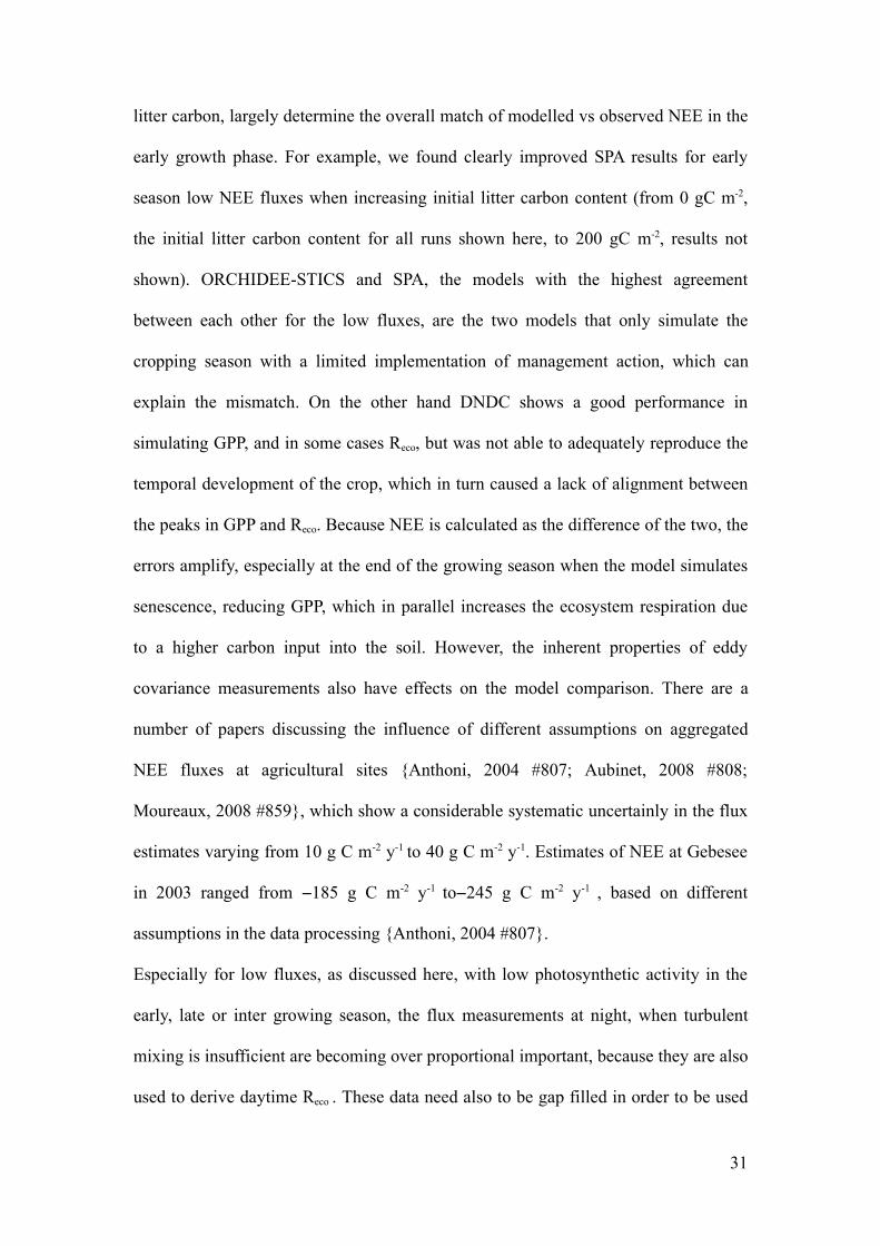
litter carbon, largely determine the overall match of modelled vs observed NEE in the

early growth phase. For example, we found clearly improved SPA results for early

season low NEE fluxes when increasing initial litter carbon content (from 0 gC m-2,

the initial litter carbon content for all runs shown here, to 200 gC m-2, results not

shown). ORCHIDEE-STICS and SPA, the models with the highest agreement

between each other for the low fluxes, are the two models that only simulate the

cropping season with a limited implementation of management action, which can

explain the mismatch. On the other hand DNDC shows a good performance in

simulating GPP, and in some cases Reco, but was not able to adequately reproduce the

temporal development of the crop, which in turn caused a lack of alignment between

the peaks in GPP and Reco. Because NEE is calculated as the difference of the two, the

errors amplify, especially at the end of the growing season when the model simulates

senescence, reducing GPP, which in parallel increases the ecosystem respiration due

to a higher carbon input into the soil. However, the inherent properties of eddy

covariance measurements also have effects on the model comparison. There are a

number of papers discussing the influence of different assumptions on aggregated

NEE fluxes at agricultural sites {Anthoni, 2004 #807; Aubinet, 2008 #808;

Moureaux, 2008 #859}, which show a considerable systematic uncertainly in the flux

estimates varying from 10 g C m-2 y-1 to 40 g C m-2 y-1. Estimates of NEE at Gebesee

in 2003 ranged from 185 g C m" -2 y-1 to 245 g C m" -2 y-1 , based on different

assumptions in the data processing {Anthoni, 2004 #807}.

Especially for low fluxes, as discussed here, with low photosynthetic activity in the

early, late or inter growing season, the flux measurements at night, when turbulent

mixing is insufficient are becoming over proportional important, because they are also

used to derive daytime Reco . These data need also to be gap filled in order to be used

31

to calculate daily means. The error introduced by gap filling is as follows: at daytime,

maximum observed errors were ±0.20 g C m 2" , and at night time the maximum was

±0.14 g C m 2 " per percentage of day filled {Falge, 2001 #549}. The percentage of

gap-filled half hourly data range from as low as 29.2% for 302 days at Gebesee 2005

up to 58.9% for 347 days at Klingenberg 2005 which could explain the inconsistent

reproduction of these fluxes by the models.

5. Conclusions

Overall, the models tested in this study show an acceptable to very good performance

when simulating NEE with significant associations and efficiencies above zero,

beside DNDC in Grignon in 2006. All models have problems in reproducing fluxes

between 2 and -2 g C m2 day-1, most probably due to a combination of a lack of

accuracy in simulating the correct temporal sequence of development stages,

problems to capture the ecosystem respiration flux and not considering all

management actions.

For European scale application, models likes SPA and ORCHIDEE-STICS are highly

accurate in simulating net carbon fluxes (NEE) and water fluxes. However, they are

only able to simulate the seasonal carbon balance of a limited number of crops with a

limited consideration of management. Thus they are not yet capable of evaluating the

wide range of mitigation options envisaged for agriculture in the context of climate

change {IPCC, 2007 #761; Smith, 2008 #735}. They are also not able to simulate

accurately annual carbon budgets because they do not consider post-harvest effects

(such as intercrop or re-growth).

32

On the other hand models like CERES-EGC and DNDC are less accurate in

simulating NEE and especially poor in reproducing latent heat fluxes. They are

however capable of simulating mitigation options because they can simulate full crop

rotations and associated management effects. CERES-EGC and DNDC also consider

other greenhouse gases like N2O, and in case of DNDC and CH4, that might affect the

GHG balance. DNDC has, in this case, the widest range of crop/management options

under irrigated and non-irrigated conditions {Leip, 2008 #716} but shows the lowest

accuracy in the carbon daily flux simulations. Both models, however, fail to

accurately present the associated water fluxes, and this might limit their ability to

simulate possible drought effects, which will have an increasing importance in future

due to climate change {Seneviratne, 2002 #851; Salinger, 2005 #852; Falloon #853}.

Finally, this model comparison shows that multiply constrained model evaluation is

clearly improved with high temporal resolution data sources, such as those from eddy

flux data, in combination with detailed management information, such as that

provided at the CarboEurope IP sites.

6. Acknowledgements

Pete Smith is a Royal Society-Wolfson Research Merit Award holder. The

CarboEurope IP project was funded by the EU’s Sixth Framework Programme for

Research and Technological Development. The work of the paper contributed to the

CC-Tame, Carbo-Extreme and NitroEurope IP project.

33

7. References

34

Tables:

."/"+&1&/!,"+& 3,)14),1&/!4(&"1 ! ! ! !

+")7& #"/*&6

! !B1:A5?!!?8@5 !

,5<?8<65<!

B1:A5?!?8@5 !

"A>145

B1:A5?!?8@5 !

&525?55

B1:A5?!?8@5 !

&>86<=<

B1:A5?!?8@5 !

):8<65<25>6

B1:A5?!?8@5 !

&>86<=<

B1:A5?!!?8@5 !

&525?55

C>C2;!3:><2BB! 96$*!!71HI UWNNKNN UTNNKNN UTNNKNN UTNNKNN UTNNKNN TSNNKNN VPNNKNN?>AD>=!>7!8A2:=! NKRN NKRN NKRN NKRN NKRN NKRR NKQN?>AD>=!>7!B9>>C NKSS NKSS NKSS NKSS NKSS NKRW NKTS?>AD>=!>7!A>>C NKNS NKNS NKNS NKNS NKNS NKNU NKNSC>C2;!?;2=C!#L,!A2D> TVKNN QTKNW QTKNW QTKNW QTKNW SPKNN VRKNN8A2:=!#L,!A2D> QSKNN PVKNN PVKNN PVKNN PVKNN QUKNN RNKNNA>>C!#L,!A2D> ONNKNN SRKNN SRKNN SRKNN SRKNN USKNN OTNKNNB9>>C!#L,!A2D> ONNKNN RRKNN RRKNN RRKNN RRKNN USKNN OTNKNNF2C6A!A6@E:A6<6=C 96!C1@5>G96!28=F PNNKN OSNKN OSNKN OSNKN OSNKN SNKN ONNKN<2G!*"( ;JG;J UKN UKN UKN UKN UKN RKS SKN<2G!96:89C ; NKU NKU NKU NKU NKU PKR OKNC96A<2;!568A66!52HB K# PRNN PRNN PRNN PRNN PTNN PRNN PSNN

Tab. 1 The site specific crop parameters used to run the DNDC model for the site comparison

0)1&! $/-. 2+&!.&/)-% +-%&*

35

! ! ?@1>@ 5<4$,

0#%.%/

/-

"

,.#'($%

%

$+$

#

-6=B:=86= F:=C6A!F962C OWLONLPNNT OTLNULPNNU PUN G G G&A:8=>= <2:I6 NWLNSLPNNS PVLNWLPNNS ORP G G G

F:=C6A!F962C PVLONLPNNS ORLNULPNNT PSW G G G G"EA256 F:=C6A!F962C PULONLPNNS PWLNTLPNNT PRS G G G G);:=86=36A8 F:=C6A!F962C PSLNWLPNNS NTLNWLPNNT QRT G G G&636B66 F:=C6A!32A;6H OULNWLPNNR OTLNULPNNS QNP G G G G

Tab 2 The combination of sites, models and crops and the lengths of the simulation period for the comparison in days of the year (DOY)

0)1& '35 ! +-%&* ! ! ! ! ! ! ! ! ! ! ! ! !

$,$# #%/%0M%&# -%/#'($%%M01(#0 0." B:C6!<62=! ! 3>8@5>81 !% >! ED!6#!;HJ !% > ED!6#;HJ !% !!!!> ED!6#;HJ % !> ED!6#!;HJ % >

-6=B:=86=!PNNU ,%% NJQQ NJRS MOPU ," ," ," NJST NJSR OPS NJU NJST PP NJSQ NJSP&.. NJTP NJSU ," ," NJSV NJRQ NJSP NJSR NJSU NJSO

/64> NJO NJS ," ," NJOR NJTT MNJNT NJTR NJNT NJTN%C2 MNJOQ NJRO ," ," NJPU NJTV NJP NJTS NJOO NJSV

&A:8=>=!PNNS ,%% NJPS NJPV MPNU NJVS NJR OVS NJPW NJSW MOVW ," ," ," NJRT NJRP&.. NJUT NJSO ," ," NJSQ NJSR ," ," NJTS NJSQ

/64> MP NJTO ," ," NJQV NJUO ," ," MNJVO NJTT%C2 NJNV NJR NJUP NJQU NJSP NJSU ," ," NJRR NJRS

&A:8=>=!PNNT ,%% MNJOS NJQP MPNR NJVR NJT ONW NJVP NJUP PP NJVU NJUO RT NJSO NJSV&.. NJQO NJRW ," ," NJVQ NJSW NJVU NJSO NJTU NJSQ

/64> MOJUW NJPW ," ," NJTR NJUO NJRQ NJTS MNJPR NJSS

36

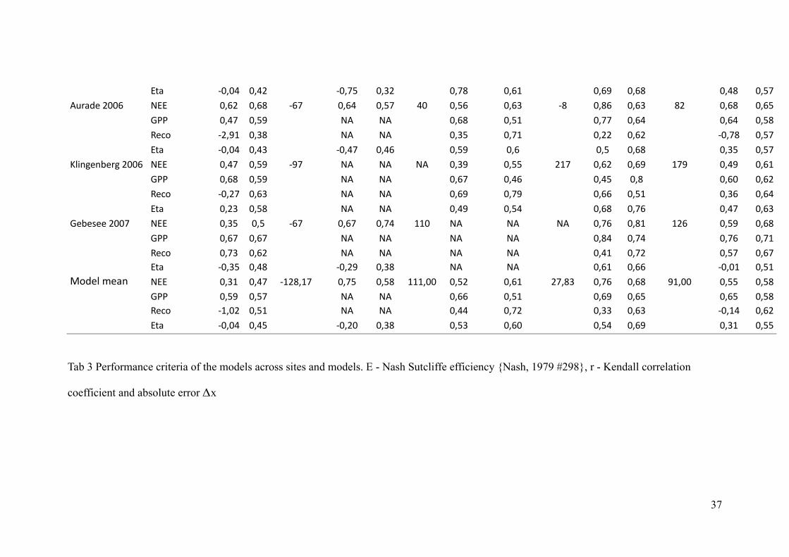
%C2 MNJNR NJRP MNJUS NJQP NJUV NJTO NJTW NJTV NJRV NJSU"EA256!PNNT! ,%% NJTP NJTV MTU NJTR NJSU RN NJST NJTQ MV NJVT NJTQ VP NJTV NJTS

&.. NJRU NJSW ," ," NJTV NJSO NJUU NJTR NJTR NJSV/64> MPJWO NJQV ," ," NJQS NJUO NJPP NJTP MNJUV NJSU

%C2 MNJNR NJRQ MNJRU NJRT NJSW NJT NJS NJTV NJQS NJSU);:=86=36A8!PNNT ,%% NJRU NJSW MWU ," ," ," NJQW NJSS POU NJTP NJTW OUW NJRW NJTO

&.. NJTV NJSW ," ," NJTU NJRT NJRS NJV NJTN NJTP/64> MNJPU NJTQ ," ," NJTW NJUW NJTT NJSO NJQT NJTR

%C2 NJPQ NJSV ," ," NJRW NJSR NJTV NJUT NJRU NJTQ&636B66!PNNU ,%% NJQS NJS MTU NJTU NJUR OON ," ," ," NJUT NJVO OPT NJSW NJTV

&.. NJTU NJTU ," ," ," ," NJVR NJUR NJUT NJUO/64> NJUQ NJTP ," ," ," ," NJRO NJUP NJSU NJTU%C2 MNJQS NJRV MNJPW NJQV ," ," NJTO NJTT MNJNO NJSO

+>56;!<62= ,%% NJQO NJRU MOPVJOU NJUS NJSV OOOJNN NJSP NJTO PUJVQ NJUT NJTV WOJNN NJSS NJSV&.. NJSW NJSU ," ," NJTT NJSO NJTW NJTS NJTS NJSV/64> MOJNP NJSO ," ," NJRR NJUP NJQQ NJTQ MNJOR NJTP

! %C2 ! MNJNR NJRS ! MNJPN NJQV ! NJSQ NJTN ! NJSR NJTW ! NJQO NJSS

Tab 3 Performance criteria of the models across sites and models. E - Nash Sutcliffe efficiency {Nash, 1979 #298}, r - Kendall correlation

coefficient and absolute error x#

37

Figures:

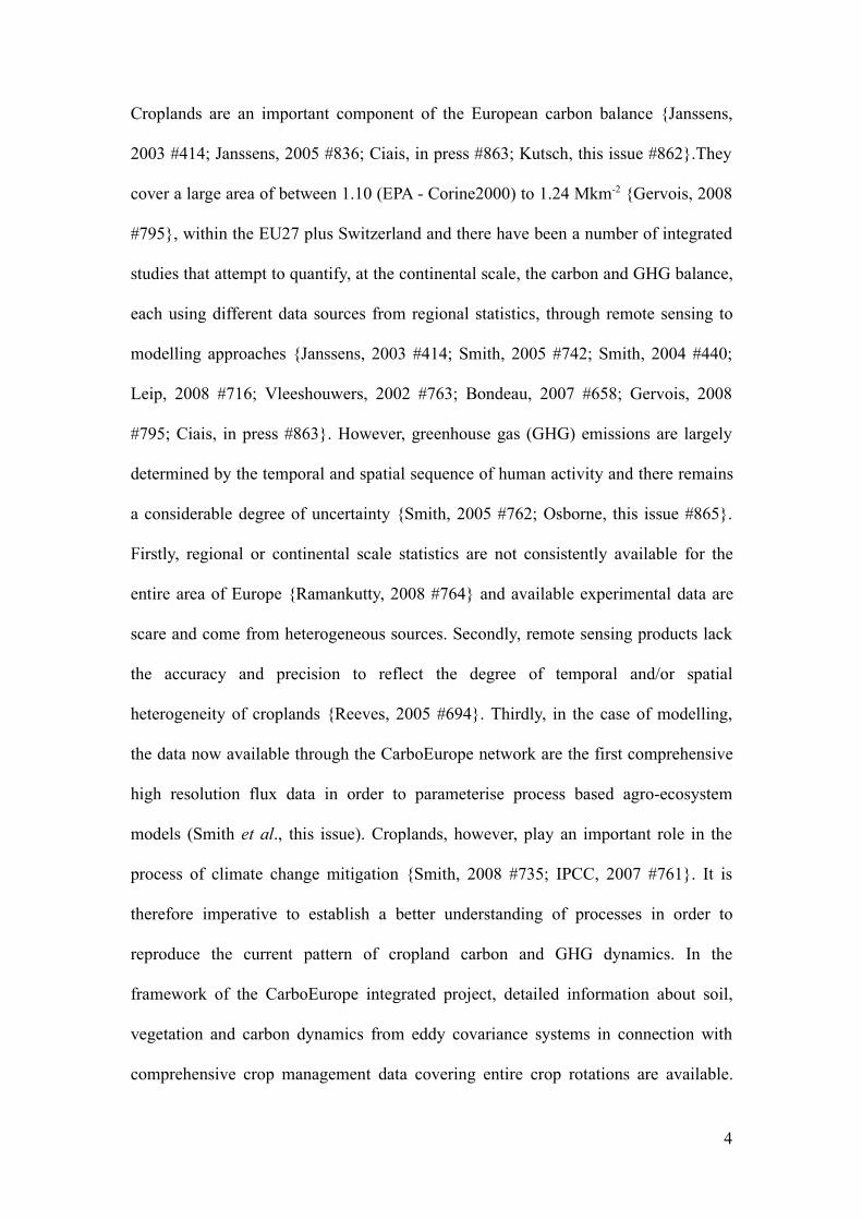
Fig. 1 The scatter plots of simulated versus measured NEE for the site Oensingen,

winter wheat, for the year 2007. The grey line indicates the lowess regression. The

numbers in right hand site panel are Kendall correlations coefficients. The size of the

number indicates the strength of the association. Noticeable is the change in the

regression for low fluxes between -2 gC m2 day-1 - 2 gC m-2day-1

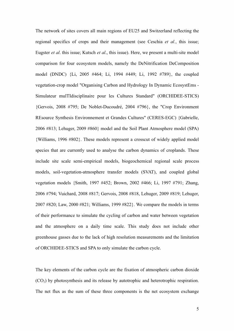
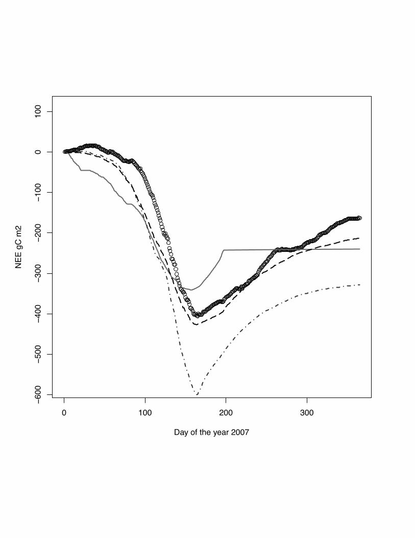
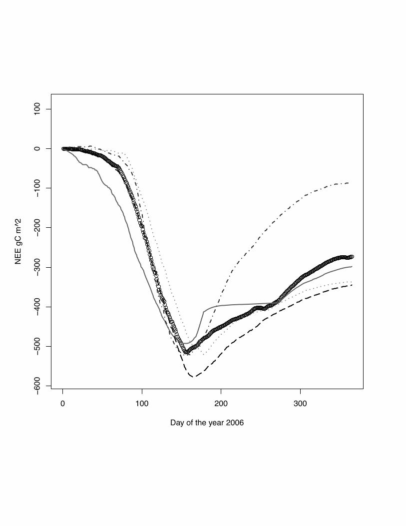
Fig. 2 Cumulative NEE for the year 2007 at the site Oensingen, winter wheat. DNDC

model: grey solid line, ORCHIDEE-STICS model: dark grey dash dot line, SPA -

black dash line, measurements indicated by open circles. In this case ORCHIDEE-

STICS is well below the measured NEE even before the end of the cropping season

(DOY 190).

Fig 3 The scatter plots of simulated versus measured NEE for the site Grignon, maize,

2005. The grey line indicates the lowess regression. The numbers in right hand site

panel are Kendall correlations coefficients. The size of the number indicates the

strength of the association. Noticeable is the change in the regression for low fluxes

between -2 gC m-2day-1 - 2 gC m-2day-1. There is no significant (p<0.05) correlation

for DNDC and ORCHIDEE-STICS.

Fig. 4 Cumulative NEE for the year 2005 at the site Grignon, maize. DNDC model:

grey solid line, ORCHIDEE-STICS model: dark grey dash dot line, CERES-EGC -

38

grey dots, measurements indicated by open circles. All model fail to capture the

cumulative flux for the year.

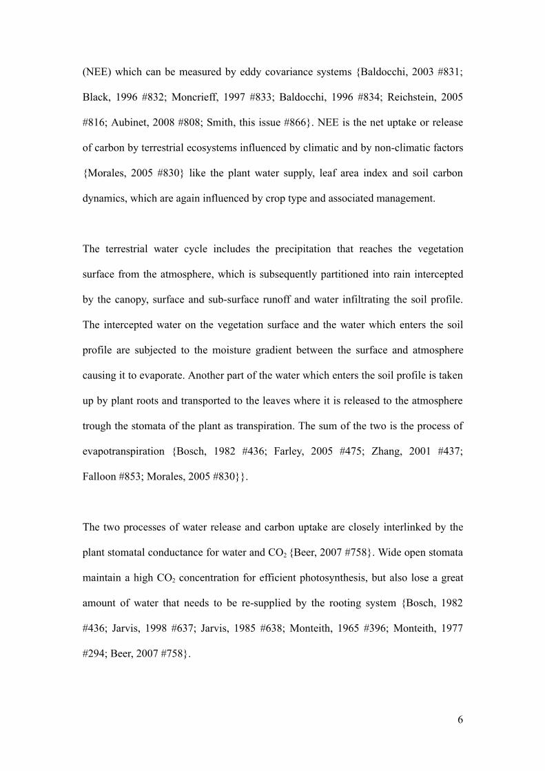
Fig 5 The scatter plots of simulated versus measured NEE for the site Grignon, winter

wheat, 2006. The grey line indicates the lowess regression. The numbers in right hand

site panel are Kendall correlations coefficients. The size of the number indicates the

strength of the association. Noticeable is the change in the regression for low

agreement for DNDC with measurements as well as the other models. The high

degree of association between ORCHIDEE-STICS and SPA indicates a similar

response to driving variables.

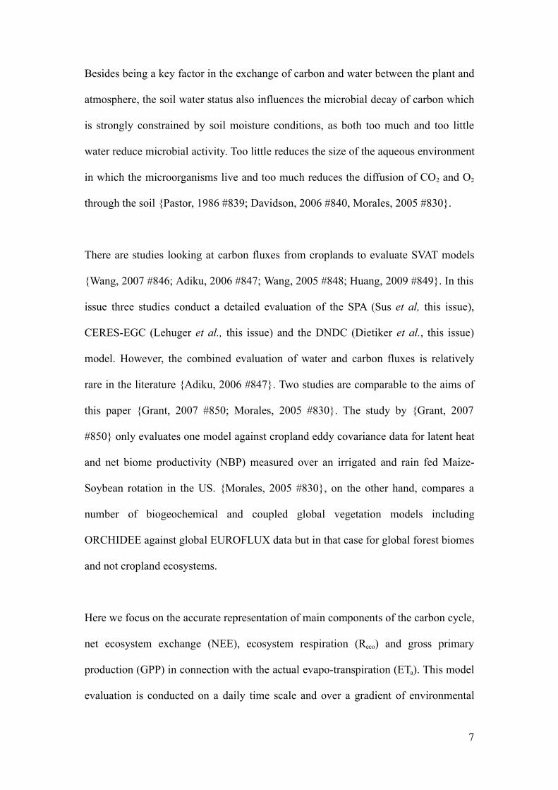
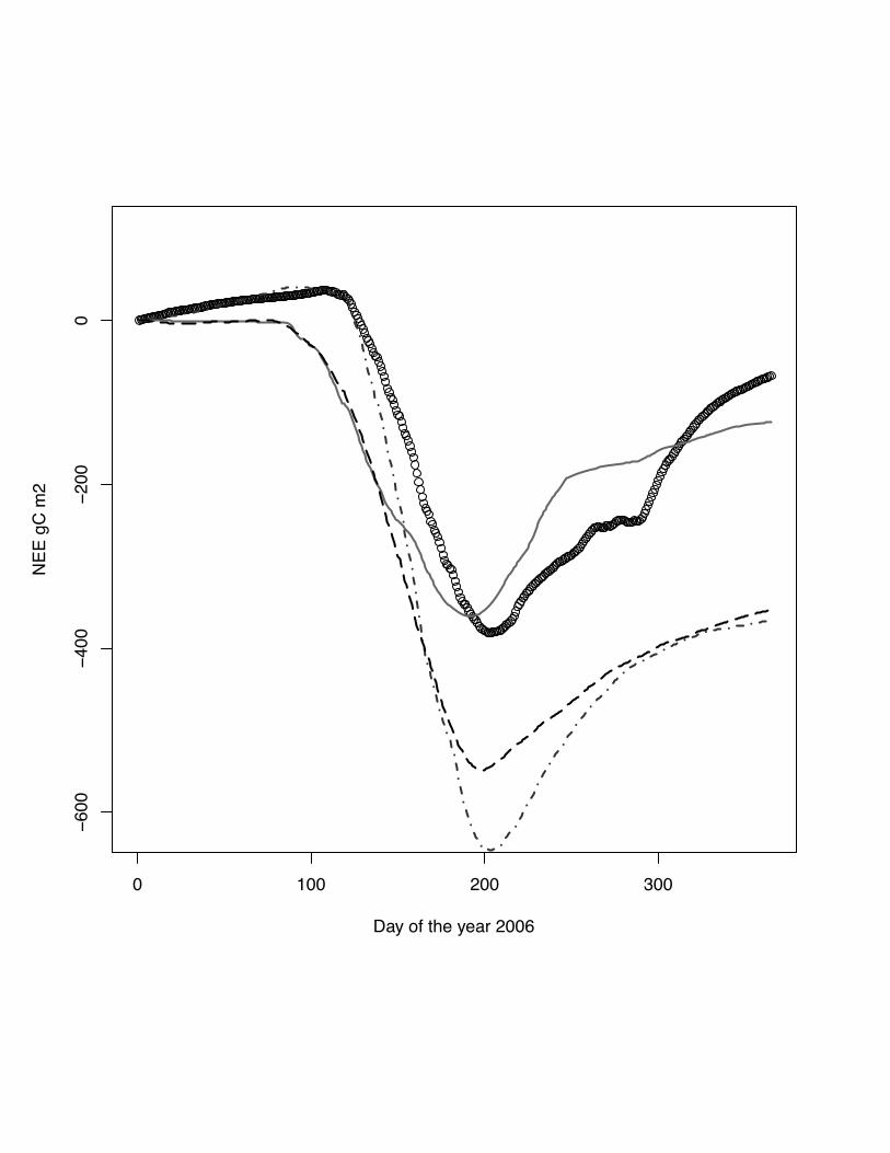
Fig. 6 Cumulative NEE for the year 2005 at the site Grignon, winter wheat. DNDC

model: grey solid line, ORCHIDEE-STICS model: dark grey dash dot line, CERES-

EGC - grey dots, SPA - black dash line, measurements indicated by open circles. Very

pronounced in the case the missing phase alignment between DNDC simulations and

observations. All models beside CERES-EGC are close to the measured cumulative

NEE.

Fig 7 The scatter plots of simulated versus measured NEE for the site Aurade, winter

wheat, 2006. The grey line indicates the lowess regression. The numbers in right hand

site panel are Kendall correlations coefficients. The size of the number indicates the

strength of the association. IN this case all model capture the NEE with good levels of

association.

39

Fig. 8 Cumulative NEE for the year 2005 at the site Aurade, winter wheat. DNDC

model: grey solid line, ORCHIDEE-STICS model: dark grey dash dot line, CERES-

EGC - grey dots, SPA - black dash line, measurements indicated by open circles.

Beside capturing the daily dynamic of fluxes (fig 7) ORCHIDEE-STICS fails to

capture the fluxes after the growing season.

Fig 9 The scatter plots of simulated versus measured NEE for the site Klingenberg,

winter wheat, 2006. The grey line indicates the lowess regression. The numbers in

right hand site panel are Kendall correlations coefficients. The size of the number

indicates the strength of the association. Again apparent, the different interpretation of

small fluxes between models and measurements as well as between models.

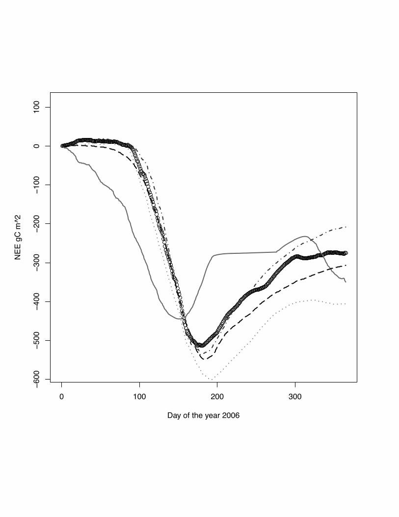
Fig. 10 Cumulative NEE for the year 2005 at the site Klingenberg, winter wheat.

DNDC model: grey solid line, ORCHIDEE-STICS model: dark grey dash dot line,

SPA - black dash line, measurements indicated by open circles. Here DNDC captures

again the cumulative flux better than the two other models.

Fig 11 The scatter plots of simulated versus measured NEE for the site Gebesee,

winter barley, 2006. The grey line indicates the lowess regression. The numbers in

right hand site panel are Kendall correlations coefficients. The size of the number

indicates the strength of the association.

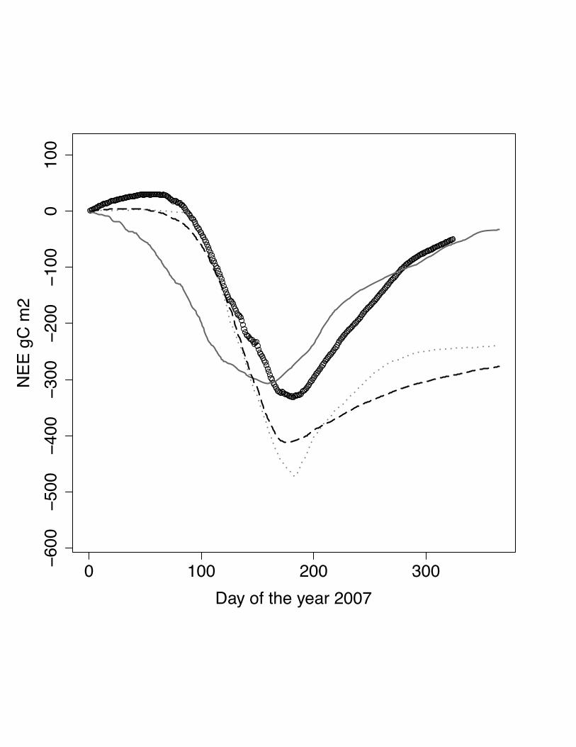
Fig. 12 Cumulative NEE for the year 2005 at the site Gebesee, winter barley. DNDC

model: grey solid line, CERES-EGC - grey dots, SPA - black dash line, measurements

40

indicated by open circles. The DNDC model is again able to capture the cumulative

flux even so it shows a strong temporal misalignment.

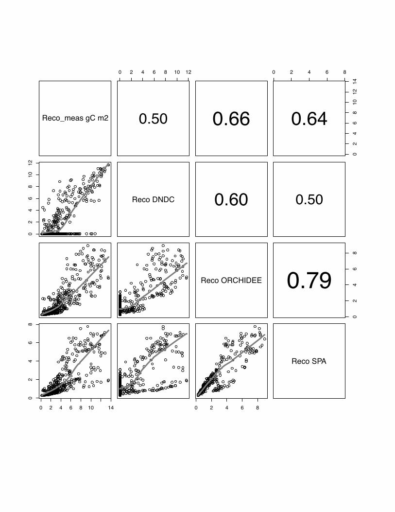
Fig 13 The scatter plots of simulated versus measured Reco for the Oensingen, winter

wheat, for the year 2007. The grey line indicates the lowess regression. The numbers

in right hand site panel are Kendall correlations coefficients. The size of the number

indicates the strength of the association. We observe a strong mismatch for the low

fluxes especially for DNDC but also for the other models indicated by the change in

the lowess fit function.

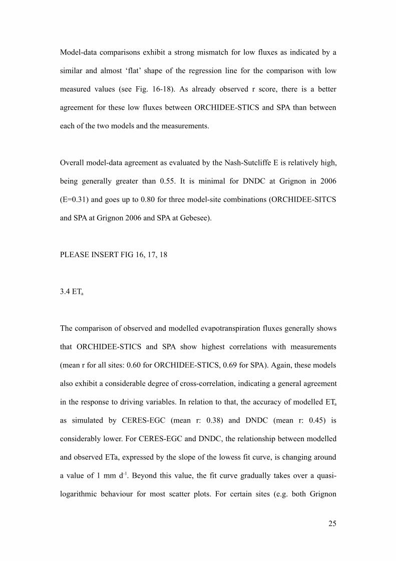
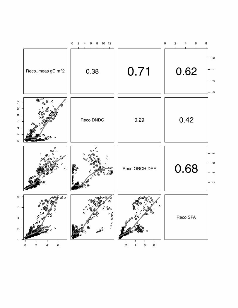
Fig 14 The scatter plots of simulated versus measured Reco for the Aurade, winter



indicates the strength of the association. The pattern of lack of fit for small fluxes

reappears now more pronounced for ORCHIDEE-STICS and SPA as in fig 13.

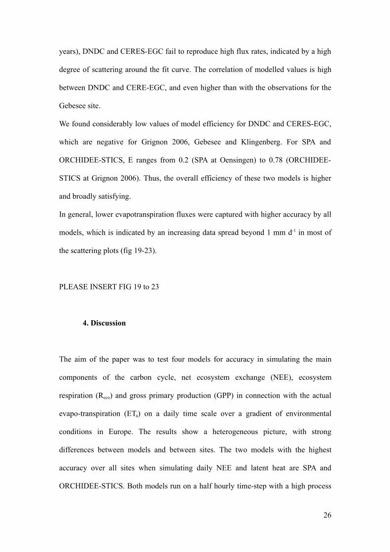
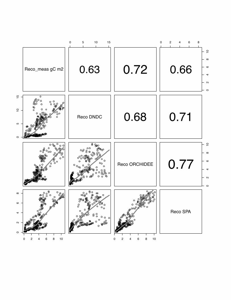
Fig 15 The scatter plots of simulated versus measured Reco for the Klingenberg, winter



indicates the strength of the association. The misfit of small fluxes observed for the

two other sites is apparent but less pronounced in this case.

Fig 16 The scatter plots of simulated versus measured GPP for the Oensingen, winter



41

indicates the strength of the association. There is a good reproduction of GPP by the

models and a less pronounced small flux disagreement. Interesting here the high

agreement between ORCHIDEEE-STICS and SPA indicating, again, the high

similarity of the model response to the external drivers.

Fig 17 The scatter plots of simulated versus measured GPP for the Grignon, winter



indicates the strength of the association. At this site we now also observe a small flux

inconsistency between measurements and models as DNDC and the two other models.

Very pronounces again the agreement between SPA and ORCHIDEE-STICS.

Fig 18 The scatter plots of simulated versus measured GPP for the Klingenberg,

winter wheat, for the year 2006. The grey line indicates the lowess regression. The

numbers in right hand site panel are Kendall correlations coefficients. The size of the

number indicates the strength of the association. The models exhibit a similar

behaviour as we saw in the other plots with an overall moderate to good agreement.

Fig 19 The scatter plots of simulated versus measured ETa for the Oensingen, winter



indicates the strength of the association. Here the two SVAT models have the best

association with the measures latent heat flux. DNDC has again problems to

reproduce low fluxes but is still able to simulate high fluxes.

42

Fig 20 The scatter plots of simulated versus measured ETa for the Grignon, maize, for

the year 2005. The grey line indicates the lowess regression. The numbers in right

hand site panel are Kendall correlations coefficients. The size of the number indicates

the strength of the association. In this case DNDC and CERES-EGC are not able to

simulate higher fluxes.

Fig 21 The scatter plots of simulated versus measured ETa for the Grignon, winter



indicates the strength of the association. CERES-EGC has together with DNDC

problems to reproduce high flux rates as observed before for this site.

Fig 22 The scatter plots of simulated versus measured Reco for the Aurade, winter



indicates the strength of the association. Apparent again, a lack of fit for DNDC for

higher flux rates.

Fig 23 The scatter plots of simulated versus measured ETa for the Gebesee, winter

barley, for the year 2007. The grey line indicates the lowess regression. The numbers


indicates the strength of the association. We observe the same pattern again, CERES-

EGC and DNDC fail to simulate the higher flux rates.

43

0 100 200 300

600

500

400

300

200

100

010

0

Day of the year 2007

NEE

gC m

2

0 100 200 300

600

500

400

300

200

100

010

0


NEE

gC m

2

0 100 200 300

600

400

200

0


NEE

gC m

2

0 100 200 300

600

500

400

300

200

100

010

0


NEE

gC m

^2

0 100 200 300

600

500

400

300

200

100

010

0


NEE

gC m

^2

0 100 200 300

500

400

300

200

100

010

0


NEE

gC m

^2

Reco_meas gC m2

0 2 4 6 8 10 12

0.50 0.66

0 2 4 6 8

02

46

810

1214

0.64

02

46

810

12

Reco DNDC 0.60 0.50

Reco ORCHIDEE

02

46

8

0.79

0 2 4 6 8 10 14

02

46

8

0 2 4 6 8

Reco SPA

Reco_meas gC m2

0 5 10 15

0.63 0.72

0 2 4 6 8

02

46

810

0.66

05

1015

Reco DNDC 0.68 0.71

Reco ORCHIDEE

02

46

810

0.77

0 2 4 6 8 10

02

46

8

0 2 4 6 8 10

Reco SPA

Reco_meas gC m^2

0 2 4 6 8 10 12

0.38 0.71

0 2 4 6 8

02

46

0.62

02

46

810

12

Reco DNDC 0.29 0.42

Reco ORCHIDEE

24

68

0.68

0 2 4 6

02

46

8

2 4 6 8

Reco SPA

NEEmeas gC m2

6 4 2 0 2 4

0.50 0.74

8 6 4 2 0 2

86

42

02

4

0.81

64

20

24

NEE DNDC 0.52 0.60

NEE CERES

84

02

4

0.75

8 6 4 2 0 2 4

86

42

02

8 4 0 2 4

NEE SPA

NEEmeas gC m2

6 4 2 0 2 4 6

0.59 0.55

10 6 4 2 0 2

105

05

0.62

64

20

24

6

NEE DNDC 0.60 0.74

NEE ORCHIDEE

1510

50

5

0.71

10 5 0 5

106

42

02

15 10 5 0 5

NEE SPA

NEEmeas gC m^2

5 0 5

0.32 0.60

10 5 0

0.72

105

0

0.71

50

5

NEE DNDC 0.35 0.32 0.30

NEE CERES 0.68

106

22

0.69

105

0

NEE ORCHIDEE 0.88

10 5 0 10 6 2 2 8 4 0 2 4

84

02

4

NEE SPA

NEEmeas gC m2

4 2 0 2 4

0.45 0.54

8 6 4 2 0 2 4

105

05

0.56

42

02

4

NEE DNDC 0.62 0.59

NEE ORCHIDEE

1510

50

5

0.82

10 5 0 5

86

42

02

4

15 10 5 0 5

NEE SPA

NEEmeas gC m^2

10 5 0 5

0.28 0.59

10 5 0 5

1510

50

5

0.40

105

05

NEE DNDC 0.28 0.074

NEE CERES

1510

50

0.50

15 10 5 0 5

105

05

15 10 5 0

NEE ORCHIDEE

NEEmeas gC m^2

5 0 5

0.68 0.57

10 5 0 5

0.63

106

22

0.63

50

5

NEE DNDC 0.49 0.54 0.51

NEE CERES 0.67

84

02

0.71

105

05

NEE ORCHIDEE 0.82

10 6 2 2 8 4 0 2 8 4 0 2

84

02

NEE SPA

GPPmeas gC m2

14 10 6 2 0

0.57 0.43

15 10 5 0

2015

105

0

0.54

1410

64

20

GPP DNDC 0.63 0.76

GPP ORCHIDEE

2520

1510

50

0.83

20 15 10 5 0

1510

50

25 20 15 10 5 0

GPP SPA

GPPmeas gC m2

15 10 5 0

0.59 0.46

15 10 5 0

1510

50

0.45

1510

50

GPP DNDC 0.51 0.66

GPP ORCHIDEE

2520

1510

50

0.63

15 10 5 0

1510

50

25 15 5 0

GPP SPA

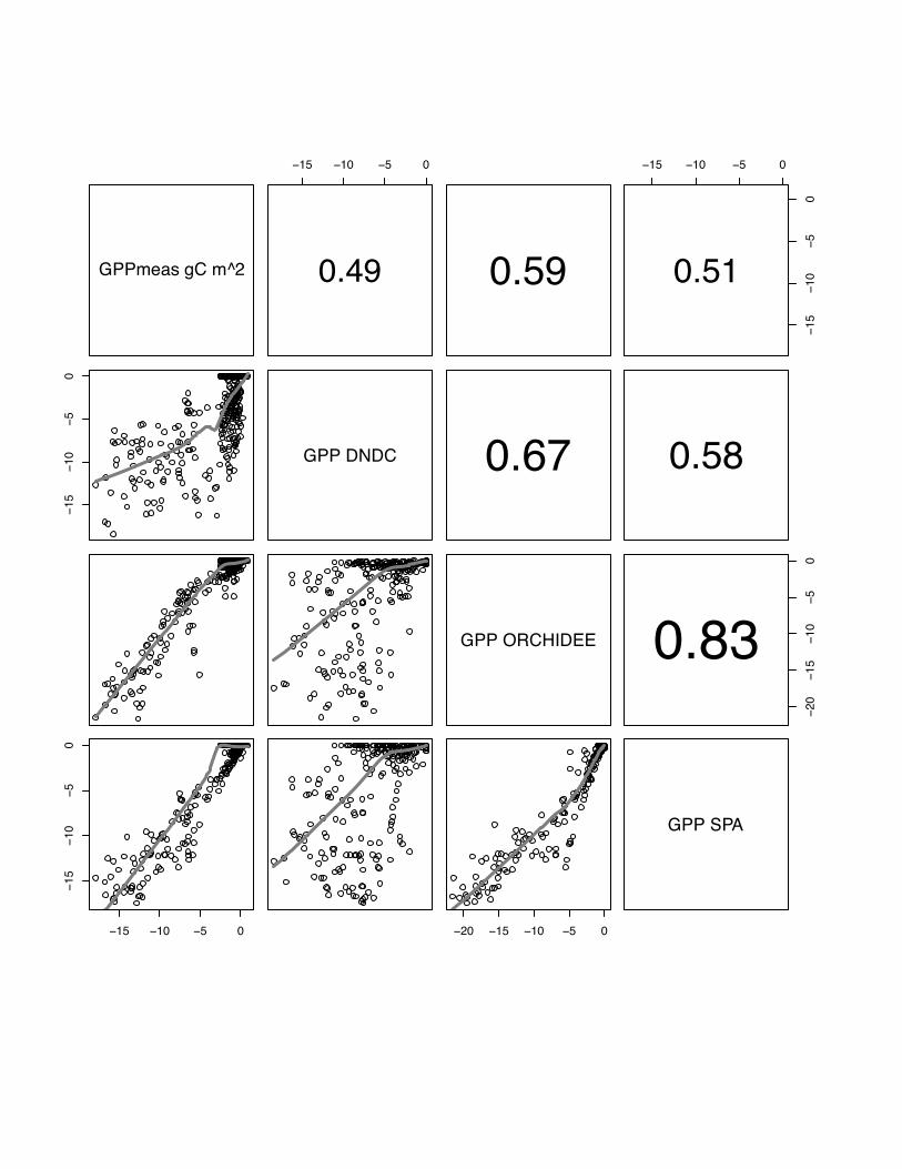
GPPmeas gC m^2

15 10 5 0

0.49 0.59

15 10 5 0

1510

50

0.51

1510

50

GPP DNDC 0.67 0.58

GPP ORCHIDEE

2015

105

0

0.83

15 10 5 0

1510

50

20 15 10 5 0

GPP SPA

ETa meas mm

0 1 2 3 4 5

0.41 0.68

0 1 2 3 4 5

01

23

45

6

0.65

01

23

45

ETa DNDC 0.39 0.39

ETa ORCHIDEE

01

23

4

0.70

0 1 2 3 4 5 6

01

23

45

0 1 2 3 4

ETa SPA

ETa meas mm

0 1 2 3 4 5

0.48 0.38

0 1 2 3 4

01

23

4

0.66

01

23

45

ETa DNDC 0.47 0.49

ETa CERES

01

23

45

0.34

0 1 2 3 4

01

23

4

0 1 2 3 4 5

ETa SPA

ETa meas mm

0 1 2 3 4

0.42 0.32

0 1 2 3 4

0.61

01

23

45

0.68

01

23

4

ETa DNDC 0.35 0.38 0.32

ETa CERES 0.23

01

23

4

0.33

01

23

4

ETa ORCHIDEE 0.61

0 1 2 3 4 5 0 1 2 3 4 0 1 2 3 4

01

23

4

ETa SPA

ETa meas mm

0 1 2 3 4

0.43 0.46

0 1 2 3 4

0.60

01

23

4

0.68

01

23

4

ETa DNDC 0.38 0.47 0.42

ETa CERES 0.46

01

23

45

0.41

01

23

4

ETa ORCHIDEE 0.65

0 1 2 3 4 0 1 2 3 4 5 0 1 2 3 4 5

01

23

45

ETa SPA

ETa meas mm

0 1 2 3 4 5

0.40 0.37

0.0 1.0 2.0 3.0

01

23

45

6

0.57

01

23

45

ETa DNDC 0.18 0.30

ETa CERES

0.0

1.0

2.0

3.0

0.21

0 1 2 3 4 5 6

0.0

1.0

2.0

3.0

0.0 1.0 2.0 3.0

ETa ORCHIDEE

Documents

The carbon balance of European croplands: a cross …homepage.usys.ethz.ch/eugsterw/publications/pdf/Wattenbach.2010...The carbon balance of European croplands: a cross-site comparison