The Case for Flexible Exchange Rates

in a Great Recession

Giancarlo Corsetti, Keith Kuester and Gernot J. Muller∗

June 3, 2016

Abstract

We analyze macroeconomic stabilization in a small open economy which faces a largerecession in the rest of the world. We show analytically that for the economy to remainisolated from the external shock, the exchange rate must depreciate not only to offsetthe collapse in external demand, but also to decouple domestic prices from deflation inthe rest of the world. If monetary policy becomes constrained by the zero lower bound,the scope of exchange rate depreciation is limited and the economy is no longer isolatedfrom the shock. Still, in this case there is a “benign coincidence”: government spending isparticularly effective in stabilizing economic activity. Under fixed exchange rates, instead,the impact of the external shock is particularly severe and the effectiveness of fiscal policylimited.

Keywords: External shock, Great Recession, Exchange rate, Zero lower bound,Fiscal Multiplier, External-demand multiplier, Benign coincidence

JEL-Codes: F41, F42, E32

∗Corsetti: Cambridge University and CEPR. Kuester: University of Bonn and CEPR. Muller: Universityof Tubingen and CEPR. This paper is prepared for the SNB/IMF/IMFER conference on “Exchange Ratesand External Adjustment”. Corsetti acknowledges support from the Centre for Macroeconomics, ADEMU andthe Keynes Fellowship at Cambridge University in developing the background research. Francesco D’Ascanioprovided excellent research assistance. We also thank an anonymous referee for useful comments. The usualdisclaimer applies.

1 Introduction

The case for flexible exchange rates rests on the ability of monetary policy to adjust its

stance and let the exchange rate depreciate or appreciate in response to shocks. Hence, even

economies with floating exchange rates may suffer notably as a consequence of large external

shocks, if monetary policy becomes constrained by the the zero lower bound (ZLB) on interest

rates. Although the nature of ZLB constraint is quite different from that implied by an

exchange rate peg or participation in a currency union, the implications for macroeconomic

resilience in the face of external shocks are potentially severe.

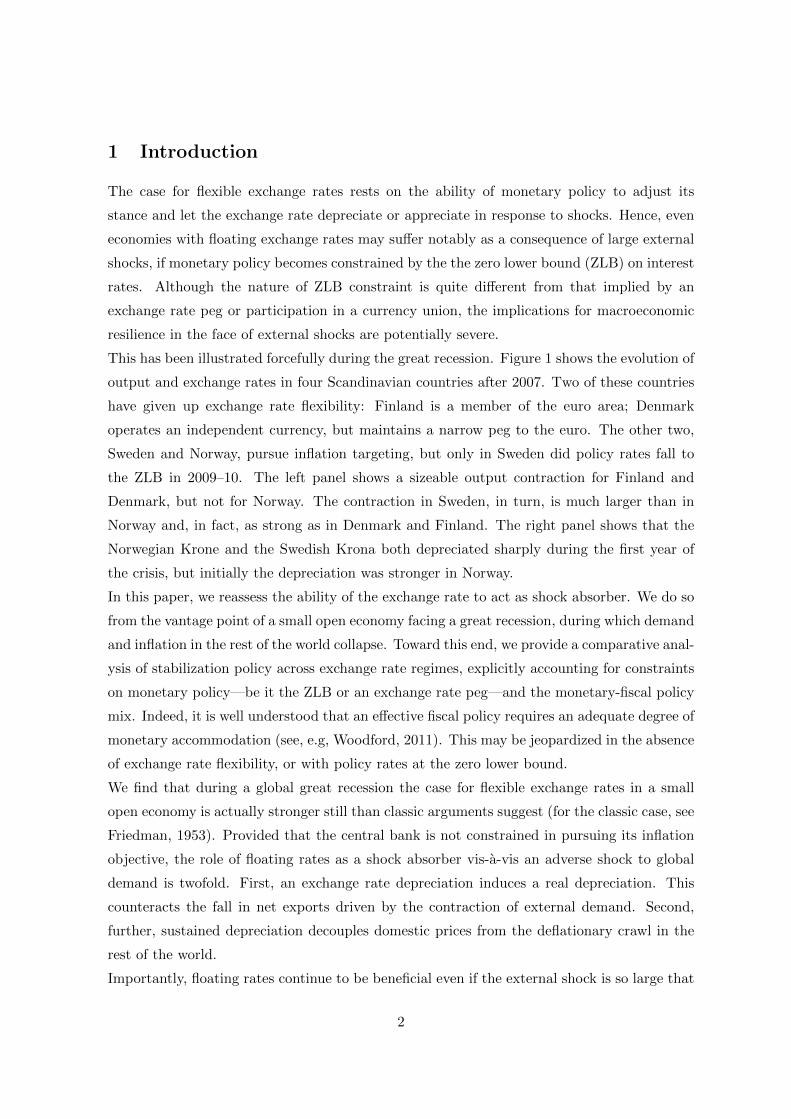
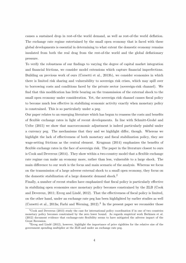
This has been illustrated forcefully during the great recession. Figure 1 shows the evolution of

output and exchange rates in four Scandinavian countries after 2007. Two of these countries

have given up exchange rate flexibility: Finland is a member of the euro area; Denmark

operates an independent currency, but maintains a narrow peg to the euro. The other two,

Sweden and Norway, pursue inflation targeting, but only in Sweden did policy rates fall to

the ZLB in 2009–10. The left panel shows a sizeable output contraction for Finland and

Denmark, but not for Norway. The contraction in Sweden, in turn, is much larger than in

Norway and, in fact, as strong as in Denmark and Finland. The right panel shows that the

Norwegian Krone and the Swedish Krona both depreciated sharply during the first year of

the crisis, but initially the depreciation was stronger in Norway.

In this paper, we reassess the ability of the exchange rate to act as shock absorber. We do so

from the vantage point of a small open economy facing a great recession, during which demand

and inflation in the rest of the world collapse. Toward this end, we provide a comparative anal-

ysis of stabilization policy across exchange rate regimes, explicitly accounting for constraints

on monetary policy—be it the ZLB or an exchange rate peg—and the monetary-fiscal policy

mix. Indeed, it is well understood that an effective fiscal policy requires an adequate degree of

monetary accommodation (see, e.g, Woodford, 2011). This may be jeopardized in the absence

of exchange rate flexibility, or with policy rates at the zero lower bound.

We find that during a global great recession the case for flexible exchange rates in a small

open economy is actually stronger still than classic arguments suggest (for the classic case, see

Friedman, 1953). Provided that the central bank is not constrained in pursuing its inflation

objective, the role of floating rates as a shock absorber vis-a-vis an adverse shock to global

demand is twofold. First, an exchange rate depreciation induces a real depreciation. This

counteracts the fall in net exports driven by the contraction of external demand. Second,

further, sustained depreciation decouples domestic prices from the deflationary crawl in the

rest of the world.

Importantly, floating rates continue to be beneficial even if the external shock is so large that

2

Output Exchange rate

90%

92%

94%

96%

98%

100%

102%

104%

Q4-2007 Q4-2008 Q4-2009 Q4-2010 Q4-2011 Q4-2012

Denmark Finland Norway Sweden

-12%

-8%

-4%

0%

4%

8%

12%

16%

20%

24%

Q4-2007 Q4-2008 Q4-2009 Q4-2010 Q4-2011 Q4-2012

DKK NOK SEK

Figure 1: Real GDP (left) and change of exchange rate (end of quarter price of euro, inlocal currency) in four Scandinavian countries. Sample period: 2007Q4–2012Q4. GDP isnormalized to 100 Percent in 2007Q4, the exchange rate is expressed in percentage changesrelative to 2007Q4. Source: OECD Economic Outlook 98 and Bundesbank.

domestic policy rates become constrained by the ZLB. Anticipating a future monetary ex-

pansion, the exchange rate in Home still depreciates (although less than in the unconstrained

case), thereby providing some isolation from the adverse developments in the rest of the world.

In addition, floating exchange rates allow fiscal stimulus to become very effective precisely

when monetary policy can deliver less stabilization—a “benign coincidence.”

The opposite holds in case of a fixed exchange rate regime. Lack of exchange rate flexibility

not only exposes the economy fully to the adverse consequences of the external demand shock.

It also amplifies the transmission of a global great recession. This is so because fixed exchange

rate anchor the domestic price level to the foreign deflationary crawl. This, in turn, pushes up

domestic real interest rates and induces a collapse of internal demand. Last but not least, an

exchange rate peg also prevents fiscal policy from having a significant and persistent effects

on domestic inflation, as the external nominal anchor keeps it tied to inflation abroad. Very

much at odds with the received wisdom, fiscal policy is not necessarily more effective in a

fixed exchange rate. Rather, the benign coincidence breaks down.

We establish these results analytically in a stylized framework as well as through model

simulations. To state our results as clearly as possible, we build on the workhorse monetary

model of a small open economy in its standard New Keynesian specification.1 Throughout

our analysis, we posit a large rise in world preferences for current savings. This shock cannot

be fully offset by appropriate monetary policy measures in the rest of the world and, thus,

1In the New Keynesian specification, the small open economy takes the global equilibrium as given butmaintains some monopoly power on its terms of trade—see, for instance, Galı and Monacelli (2005) and DePaoli (2009) which, in turn, build the New Open Economy Macroeoconomics literature (Obstfeld and Rogoff,1996).

3

causes a sustained drop in rest-of-the world demand, as well as rest-of-the world deflation.

The exchange rate regime entertained by the small open economy that is faced with these

global developments is essential in determining to what extent the domestic economy remains

insulated from both the real drag from the rest-of-the world and the global deflationary

pressure.

To verify the robustness of our findings to varying the degree of capital market integration

and financial frictions, we consider model extensions which capture financial imperfections.

Building on previous work of ours (Corsetti et al., 2013b), we consider economies in which

there is limited risk sharing and vulnerability to sovereign risk crises, which may spill over

to borrowing costs and conditions faced by the private sector (sovereign-risk channel). We

find that this modification has little bearing on the transmission of the external shock to the

small open economy under consideration. Yet, the sovereign risk channel causes fiscal policy

to become much less effective in stabilizing economic activity exactly when monetary policy

is constrained. This is so particularly under a peg.

Our paper relates to an emerging literature which has begun to reassess the costs and benefits

of flexible exchange rates in light of recent developments. In line with Schmitt-Grohe and

Uribe (2015) we show that macroeconomic adjustment is indeed particularly painful under

a currency peg. The mechanisms that they and we highlight differ, though. Whereas we

highlight the lack of effectiveness of both monetary and fiscal stabilization policy, they see

wage-setting frictions as the central element. Krugman (2014) emphasizes the benefits of

flexible exchange rates in the face of sovereign risk. The paper in the literature closest to ours

is Cook and Devereux (2014). They show within a two-country model that a flexible exchange

rate regime can make an economy more, rather than less, vulnerable to a large shock. The

main difference to our work is the focus and main scenario of the analysis. Whereas we focus

on the transmission of a large adverse external shock to a small open economy, they focus on

the domestic stabilization of a large domestic demand shock.2

Finally, a number of recent studies have emphasized that fiscal policy is particularly effective

in stabilizing open economies once monetary policy becomes constrained by the ZLB (Cook

and Devereux, 2011; Erceg and Linde, 2012). That the effectiveness of fiscal policy is limited,

on the other hand, under an exchange rate peg has been highlighted by earlier studies as well

(Corsetti et al., 2013a; Farhi and Werning, 2012).3 In the present paper we reconsider those

2Cook and Devereux (2013) study the case for international policy coordination if in one of two countriesmonetary policy becomes constrained by the zero lower bound. As regards empirical work Berkmen et al.(2012) document evidence that exchange-rate flexibility seems to have mitigated the adverse impact of theGreat Recession.

3Erceg and Linde (2012), however, highlight the importance of price rigidities for the relative size of thegovernment spending multiplier at the ZLB and under an exchange rate peg.

4

findings in circumstances where a need for effective stabilization arises from a large external

shock.

The text is organised as follows. Section 2 outlines the model by focusing on a log-linear

approximation of the equilibrium conditions. Section 3 provides a number of closed-form

results on the transmission and stabilization of a great recession under alternative policy

scenarios in the small open economy. Section 4 illustrates the quantitative relevance of these

results through model simulations. It also provides results for a modified environment with

financial friction and sovereign risk. Section 5 concludes.

2 A New Keynesian small open-economy model

We conduct our analysis in a standard New Keynesian framework, using a version of the

two-country model put forward in Corsetti et al. (2012). Both countries produce a variety of

country-specific intermediate goods, with the number of intermediate good producers in the

world normalized to unity. While international financial markets are complete, goods market

integration is incomplete due to home bias. Hence, while we assume that the law of one price

holds at the level of intermediate goods, purchasing power parity fails in the short run. The

countries have isomorphic structures, but may differ in terms of size, policies, and shocks.

We build a scenario in which a small open economy faces a great recession in the rest of the

world. For this purpose we make the following assumptions. First, the size of the domestic

economy (“Home”) in the world economy approaches zero, while the rest of the world is

consolidated in “Foreign”. As a result, Home behaves like a small open economy, while

Foreign behaves like a closed economy.4 Second, the only source of variation at the world

level is a foreign “saving shock.” This shock effectively alters the time-discount factor. Such

preference shocks often-times are used to model an exogenous variation of the intertemporal

allocation of private expenditures (for a textbook treatment see Galı, 2015). In order to

determine the effect of the shock on Home, one needs to know the effect of the shock on

foreign demand and prices. We shall, third, assume that the shock in Foreign occurs when

monetary policy in Foreign is unable to contain its effect.

Importantly, while our focus is on Home, we are explicit about the dynamics in Foreign so

that the external shock which impacts Home is fully micro-founded. As a result we may

account for the cross-equation restrictions of the model along two dimensions. First, the

saving shock in Foreign impacts Home not only via goods markets, but also via financial

markets.5 Second, the model restricts the joint dynamics of output and inflation in Foreign

4In this case Home is identical to the small open economy of Galı and Monacelli (2005), except for the factthat we allow for government consumption and restrict preferences to log-utility.

5The global fall in demand (including the demand for the Home output), and the adjustment in the world

5

during a great recession thus modelled. As we shall see, the dynamics of both of these matter

for Home.

The structure of the model is well-known. We give a detailed description in Appendix A. In

the following, instead, we provide a compact exposition, based on a log-linear approximation

of the equilibrium conditions around a deterministic and symmetric zero-inflation steady

state. Output is normalized to one. In both the appendix and the text, foreign variables are

indexed with a star. Variables carry a time-subscript, t. Variables without a hat refer to log

deviations from the steady state. Variables that carry a hat refer to deviations in levels. We

begin with Foreign and discuss the equilibrium conditions in Home afterwards.

In order to simplify the exposition, and derive tractable pencil-and-paper solutions, we ini-

tially posit that financial markets are complete across countries, and make some simplifying

assumptions. These assumptions will be relaxed later, when we resort to numerical simula-

tions, with little effect as to the qualitative conclusions of our analysis.

2.1 Foreign

Under our assumptions, Foreign operates like a closed economy. The equilibrium dynamics

of output, y∗t , inflation, π∗t , and nominal interest rates, r∗t , are driven by the dynamics of the

saving shock in Foreign, ξ∗t . We will specify a law of motion for the shock later. Conditional on

the dynamics of the shock, the evolution of the foreign economy is captured by the following

three equations. The first is the dynamic IS-equation:

y∗t = Ety∗t+1 − (r∗t − Etπ∗t+1 + Et∆ξ

∗t+1). (1)

Here Et is the expectations operator and ∆ marks the difference operator. We abstract from

government consumption in Foreign. Next, there is the New Keynesian Phillips curve:

π∗t = βEtπ∗t+1 + κ (ϕ+ 1) y∗t . (2)

Here β is the steady-state time-discount factor. κ := (1 − α)(1 − βα)/α measures the slope

of the Phillips curve, with α ∈ [0, 1) measuring the degree of price stickiness. ϕ > 0 is the

inverse of the Frisch elasticity of labor supply. The next (and last) equation for Foreign is an

instrument rule for the foreign central bank that describes monetary policy. We assume that

r∗t = max{φππ∗t − Et∆ξ∗t+1,−(1− β)}. (3)

Here, φπ > 1 is the response to inflation in normal times. Foreign can become constrained by

the zero lower bound, however, explaining the max operator. As long as the foreign central

interest rate and the price of foreign exports are all taken as given by the small open economy. Because of thefluctuation in the relative price of Home to foreign consumption, however, full insurance via complete marketsdoes not insulate Home consumption from the external shock.

6

bank can pursue rule (3) without being constrained by the ZLB, the time-discount factor

shock does not have an effect on foreign inflation or output. In this case, Foreign monetary

policy implements the flexible price allocation under which the saving shock is fully absorbed

by changes in the real rate of interest. If, instead, policy becomes constrained the flexible-

price allocation can no longer be implemented by monetary policy (alone). In this case eqs.

(1)–(2) restrict the joint dynamics of output and inflation in Foreign.

2.2 Home

While the dynamics in Foreign are independent of what happens in Home, Foreign does matter

for Home. The following set of equations describes the equilibrium dynamics in Home, given

the realization of Foreign variables. The dynamic IS-relation in Home is:

yt = Etyt+1 − (1−$)Et∆y∗t+1 − Et∆gt+1 + [1− υ −$] ∆ξ∗t+1 −$(rt − EtπH,t+1). (4)

Here gt denotes government expenditure (in units of output). In the steady state, government

consumption is zero. We allow for positive government consumption shocks in Home. Gov-

ernment spending is financed through lump-sum taxes and falls exclusively on domestically

produced goods. The term (1 − $)y∗t captures external demand for domestically produced

goods (as a function of foreign output), where $ := 1 − υ(2 − υ)(1 − σ). Here υ ∈ (0, 1)

measures the degree of openness, with a low υ implying a strong home bias (little openness),

and σ > 0 measures the trade-price elasticity of international demand.6 In deriving the above

equation, we have substituted for Home consumer-price inflation rates. Thus, what remains

in the IS-equation in Home is Home producer price inflation, πH,t.

The New Keynesian Phillips curve links inflation to expected inflation, as well as a number

of variables that determine the evolution of marginal costs in our small open economy

πHt = βEtπHt+1 + κ

{(ϕ+$−1

)yt − $−1[(1−$)y∗t + gt] +

1− υ −$$

ξ∗t

}. (5)

Note that both the dynamic IS-relation and the New Keynesian Phillips curve in Home are

a function of foreign output (that is the same as foreign consumption) as well as the foreign

saving shock, which enter the equations as separate arguments. This is because a foreign

saving shock spills over internationally through two channels. The first is a direct demand

channel: given prices, a saving shock leads to less foreign demand for domestic goods—this

is the key effect of a global recession that we wish to focus on in our analysis. The second

channel works through prices: because of home bias in consumption, for given relative prices

the fall in Foreign demand falls disproportionately on foreign-produced goods. In equilibrium,

6External demand for domestically produced goods thus increases with foreign output as long as σ < 1.

7

the relative price of foreign-produced goods must fall, which in turn crowds out demand for

domestic goods.

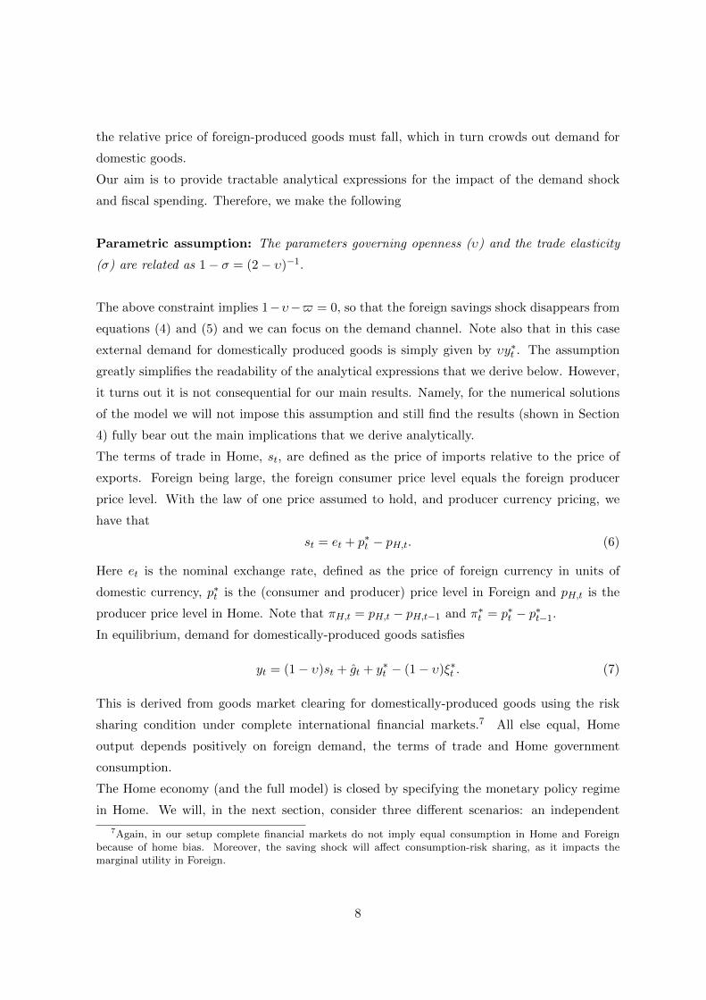
Our aim is to provide tractable analytical expressions for the impact of the demand shock

and fiscal spending. Therefore, we make the following

Parametric assumption: The parameters governing openness (υ) and the trade elasticity

(σ) are related as 1− σ = (2− υ)−1.

The above constraint implies 1−υ−$ = 0, so that the foreign savings shock disappears from

equations (4) and (5) and we can focus on the demand channel. Note also that in this case

external demand for domestically produced goods is simply given by υy∗t . The assumption

greatly simplifies the readability of the analytical expressions that we derive below. However,

it turns out it is not consequential for our main results. Namely, for the numerical solutions

of the model we will not impose this assumption and still find the results (shown in Section

4) fully bear out the main implications that we derive analytically.

The terms of trade in Home, st, are defined as the price of imports relative to the price of

exports. Foreign being large, the foreign consumer price level equals the foreign producer

price level. With the law of one price assumed to hold, and producer currency pricing, we

have that

st = et + p∗t − pH,t. (6)

Here et is the nominal exchange rate, defined as the price of foreign currency in units of

domestic currency, p∗t is the (consumer and producer) price level in Foreign and pH,t is the

producer price level in Home. Note that πH,t = pH,t − pH,t−1 and π∗t = p∗t − p∗t−1.

In equilibrium, demand for domestically-produced goods satisfies

yt = (1− υ)st + gt + y∗t − (1− υ)ξ∗t . (7)

This is derived from goods market clearing for domestically-produced goods using the risk

sharing condition under complete international financial markets.7 All else equal, Home

output depends positively on foreign demand, the terms of trade and Home government

consumption.

The Home economy (and the full model) is closed by specifying the monetary policy regime

in Home. We will, in the next section, consider three different scenarios: an independent

7Again, in our setup complete financial markets do not imply equal consumption in Home and Foreignbecause of home bias. Moreover, the saving shock will affect consumption-risk sharing, as it impacts themarginal utility in Foreign.

8

monetary policy in Home that follows the analog of the rule (3), with and without being

constrained by the ZLB, as well as the case of a currency peg.

In equilibrium, eqs. (4)–(7) determine a sequence of Home variables {yt, πH,t, pH,t, st, et, rt, gt}∞t=0,

given a specification of (i) monetary policy in Home, (ii) fiscal policy in Home, (iii) πH,t =

pH,t − pH,t−1, (iv) the sequence {y∗t , π∗t , p∗t , ξ∗t }∞t=0, as well as initial conditions (p∗−1, pH,−1).

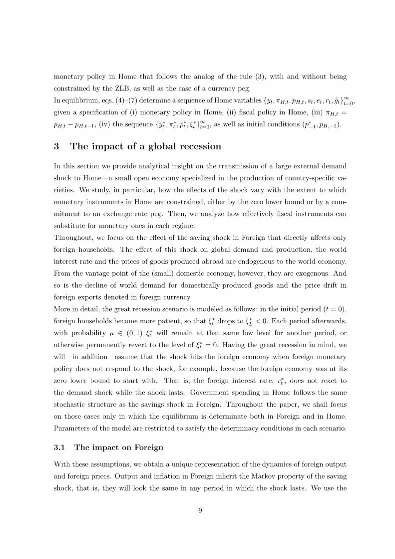
3 The impact of a global recession

In this section we provide analytical insight on the transmission of a large external demand

shock to Home—a small open economy specialized in the production of country-specific va-

rieties. We study, in particular, how the effects of the shock vary with the extent to which

monetary instruments in Home are constrained, either by the zero lower bound or by a com-

mitment to an exchange rate peg. Then, we analyze how effectively fiscal instruments can

substitute for monetary ones in each regime.

Throughout, we focus on the effect of the saving shock in Foreign that directly affects only

foreign households. The effect of this shock on global demand and production, the world

interest rate and the prices of goods produced abroad are endogenous to the world economy.

From the vantage point of the (small) domestic economy, however, they are exogenous. And

so is the decline of world demand for domestically-produced goods and the price drift in

foreign exports denoted in foreign currency.

More in detail, the great recession scenario is modeled as follows: in the initial period (t = 0),

foreign households become more patient, so that ξ∗t drops to ξ∗L < 0. Each period afterwards,

with probability µ ∈ (0, 1) ξ∗t will remain at that same low level for another period, or

otherwise permanently revert to the level of ξ∗t = 0. Having the great recession in mind, we

will—in addition—assume that the shock hits the foreign economy when foreign monetary

policy does not respond to the shock, for example, because the foreign economy was at its

zero lower bound to start with. That is, the foreign interest rate, r∗t , does not react to

the demand shock while the shock lasts. Government spending in Home follows the same

stochastic structure as the savings shock in Foreign. Throughout the paper, we shall focus

on those cases only in which the equilibrium is determinate both in Foreign and in Home.

Parameters of the model are restricted to satisfy the determinacy conditions in each scenario.

3.1 The impact on Foreign

With these assumptions, we obtain a unique representation of the dynamics of foreign output

and foreign prices. Output and inflation in Foreign inherit the Markov property of the saving

shock, that is, they will look the same in any period in which the shock lasts. We use the

9

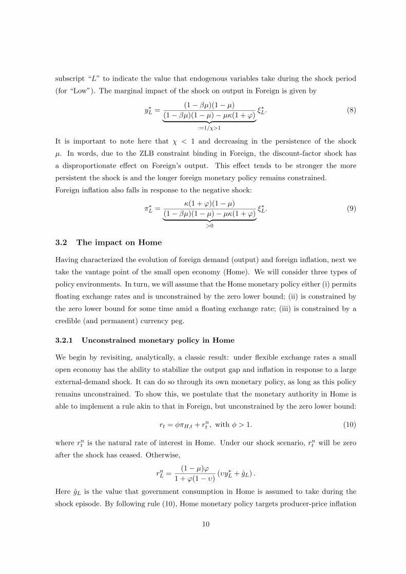
subscript “L” to indicate the value that endogenous variables take during the shock period

(for “Low”). The marginal impact of the shock on output in Foreign is given by

y∗L =(1− βµ)(1− µ)

(1− βµ)(1− µ)− µκ(1 + ϕ)︸ ︷︷ ︸:=1/χ>1

ξ∗L. (8)

It is important to note here that χ < 1 and decreasing in the persistence of the shock

µ. In words, due to the ZLB constraint binding in Foreign, the discount-factor shock has

a disproportionate effect on Foreign’s output. This effect tends to be stronger the more

persistent the shock is and the longer foreign monetary policy remains constrained.

Foreign inflation also falls in response to the negative shock:

π∗L =κ(1 + ϕ)(1− µ)

(1− βµ)(1− µ)− µκ(1 + ϕ)︸ ︷︷ ︸>0

ξ∗L. (9)

3.2 The impact on Home

Having characterized the evolution of foreign demand (output) and foreign inflation, next we

take the vantage point of the small open economy (Home). We will consider three types of

policy environments. In turn, we will assume that the Home monetary policy either (i) permits

floating exchange rates and is unconstrained by the zero lower bound; (ii) is constrained by

the zero lower bound for some time amid a floating exchange rate; (iii) is constrained by a

credible (and permanent) currency peg.

3.2.1 Unconstrained monetary policy in Home

We begin by revisiting, analytically, a classic result: under flexible exchange rates a small

open economy has the ability to stabilize the output gap and inflation in response to a large

external-demand shock. It can do so through its own monetary policy, as long as this policy

remains unconstrained. To show this, we postulate that the monetary authority in Home is

able to implement a rule akin to that in Foreign, but unconstrained by the zero lower bound:

rt = φπH,t + rnt , with φ > 1. (10)

where rnt is the natural rate of interest in Home. Under our shock scenario, rnt will be zero

after the shock has ceased. Otherwise,

rnL =(1− µ)ϕ

1 + ϕ(1− υ)(υy∗L + gL) .

Here gL is the value that government consumption in Home is assumed to take during the

shock episode. By following rule (10), Home monetary policy targets producer-price inflation

10

and adjusts policy rates to changes in the natural rate of interest. Combining the interest rate

rule specified above with equations (4) and (5), we can determine the equilibrium interest rate,

inflation and output in Home. The model shows the well-established isomorphism between

open and closed-economy settings, as is common in New Keynesian models (Clarida et al.,

2001). This is not to say that openness is irrelevant for Home. It matters for Home through

openness parameter υ. In addition, openness matters here by opening the door to external

shocks.

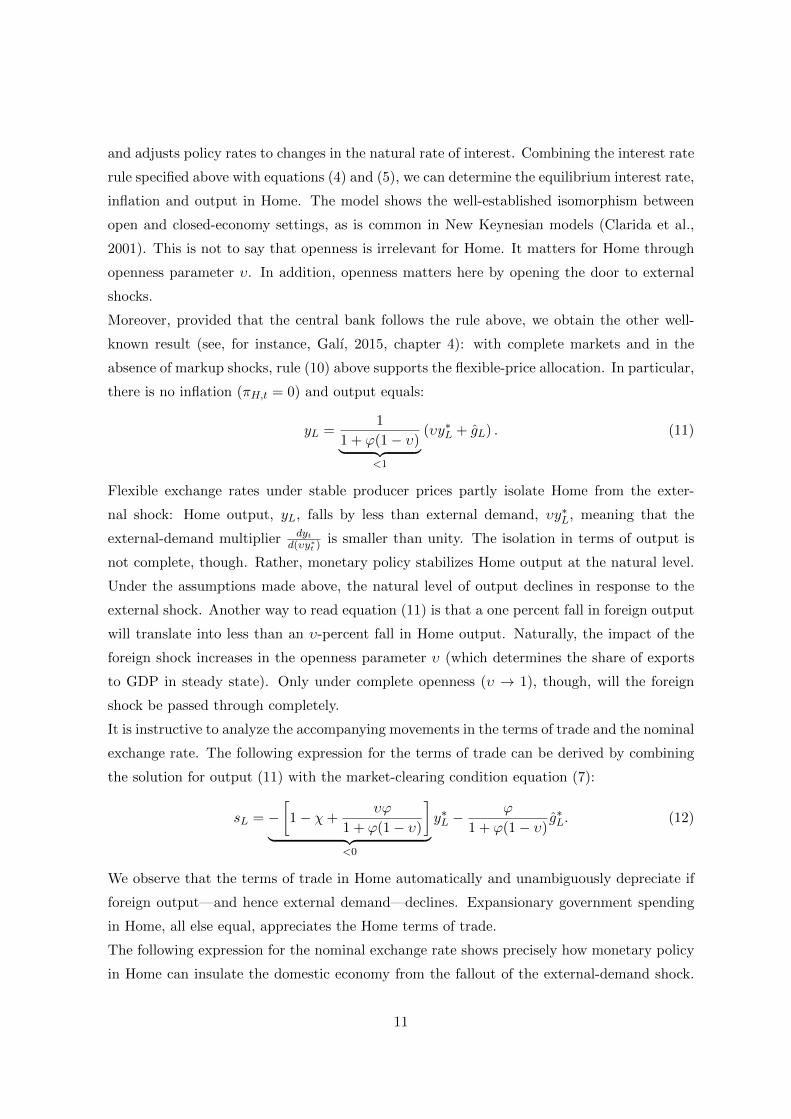
Moreover, provided that the central bank follows the rule above, we obtain the other well-

known result (see, for instance, Galı, 2015, chapter 4): with complete markets and in the

absence of markup shocks, rule (10) above supports the flexible-price allocation. In particular,

there is no inflation (πH,t = 0) and output equals:

yL =1

1 + ϕ(1− υ)︸ ︷︷ ︸<1

(υy∗L + gL) . (11)

Flexible exchange rates under stable producer prices partly isolate Home from the exter-

nal shock: Home output, yL, falls by less than external demand, υy∗L, meaning that the

external-demand multiplier dytd(υy∗t ) is smaller than unity. The isolation in terms of output is

not complete, though. Rather, monetary policy stabilizes Home output at the natural level.

Under the assumptions made above, the natural level of output declines in response to the

external shock. Another way to read equation (11) is that a one percent fall in foreign output

will translate into less than an υ-percent fall in Home output. Naturally, the impact of the

foreign shock increases in the openness parameter υ (which determines the share of exports

to GDP in steady state). Only under complete openness (υ → 1), though, will the foreign

shock be passed through completely.

It is instructive to analyze the accompanying movements in the terms of trade and the nominal

exchange rate. The following expression for the terms of trade can be derived by combining

the solution for output (11) with the market-clearing condition equation (7):

sL = −[1− χ+

υϕ

1 + ϕ(1− υ)

]︸ ︷︷ ︸

<0

y∗L −ϕ

1 + ϕ(1− υ)g∗L. (12)

We observe that the terms of trade in Home automatically and unambiguously depreciate if

foreign output—and hence external demand—declines. Expansionary government spending

in Home, all else equal, appreciates the Home terms of trade.

The following expression for the nominal exchange rate shows precisely how monetary policy

in Home can insulate the domestic economy from the fallout of the external-demand shock.

11

From (6), the nominal exchange rate, et, is given by

et = st + pH,t − p∗t , (13)

As long as monetary policy can and does pursue price stability in Home, we have pH,t = 0.

In this case, taking first differences of equation (13) implies

∆et = ∆st − π∗t . (14)

This expression makes two things apparent. First, the movement in the nominal exchange

rate perfectly insulates the domestic economy from movements in foreign inflation. In our

shock scenario, the nominal exchange rate will depreciate one-to-one with the continuing fall

in foreign’s price level, at the disinflation rate π∗L < 0. On top, in the initial period of the

shock, and only in that period, the nominal exchange rate will depreciate in excess of the

foreign deflationary crawl, so as to bring about the initial period’s depreciation of the terms

of trade.

Expression (14) thus clarifies the two dimensions along which, with monetary authorities

pursuing a regime of output gap stabilization and price stability, the nominal exchange rate

performs its role of shock absorber. First, it fully insulates agents’ expectations of domestic

inflation from the foreign deflationary drift. Second, on impact, the exchange rate depreci-

ates with the fall in external demand, contributing to real depreciation. This helps sustain

domestic employment and competitiveness. While the depreciation of the nominal exchange

rate for the sake of competitiveness will be reversed once the shock ends (and st reverts back

to zero), the same is not true of the adjustments that were due to the foreign deflationary

drift. The monetary rule (10) does not include an exchange rate target, not even in the long

run. Hence there is no implicit commitment to keep the domestic price level aligned with the

Foreign one. Rather, the nominal exchange rate will be depreciated permanently.

3.2.2 The zero lower bound constraint under flexible exchange rates in Home

In our second scenario the exchange rate regime in Home is still a float, but now also the

monetary policy in Home is assumed to be constrained when the adverse shock in Foreign

materializes. Specially, we impose that domestic policy rates are constant as long as the

foreign economy is in the shock state—for example, because Home had been at its zero lower

bound already. So, at least temporarily, the monetary authority in Home is unable to cushion

the foreign shock.

In this case the solution for domestic output is given by:

yL =

(1 +

µκϕ(1− υ)

(1− µ)(1− βµ)− µκ(1 + ϕ(1− υ))

)︸ ︷︷ ︸

:=Ξ

(υy∗L + gL) . (15)

12

One can show that

1 < Ξ <1

υ.

In other words, the external-demand multiplier is unambiguously larger than unity and thus

larger than absent the ZLB constraint in Home, compare (15) with (11). Exchange rate

flexibility alone is not sufficient to insulate the Home economy from the Foreign demand

shock.

While the drop in domestic output will never exceed the drop of output in Foreign, with the

ZLB constraint the output loss due to an external-demand shock can be large. The reason for

why the multiplier is large at the ZLB (and larger than absent the ZLB) has been extensively

explored in the context of fiscal policy (e.g., Woodford, 2011). The fall in external demand

drives down inflation and inflation expectations in a significant and sustained way, causing a

rise in (long-term) real interest rates. Specifically, the solution for inflation is given by:

πH,L =(1− µ)κϕ

(1− βµ)(1− µ)− µκ(1 + ϕ(1− υ))︸ ︷︷ ︸>0

(υy∗L + gL) , (16)

so that Home inflation will fall along with foreign demand.

Next, we turn to the accompanying movements in the terms of trade and the nominal exchange

rate. The solution for the terms of trade for the duration of the shock is given by:

sL = − 1

(1− υ)

[1− (1− υ)χ− Ξυ

]y∗L−

1− Ξ

(1− υ)︸ ︷︷ ︸>0

gL. (17)

It is instructive to compare this to the solution for the terms of trade when monetary policy

follows rule (10) in an unconstrained way, that is, to the expression in equation (12) above.

A close inspection of the terms multiplying foreign output reveals that the terms of trade

depreciate to a lesser extent in response to a drop of external demand when the ZLB binds in

Home.8 Given that the response of the terms of trade is muted at the zero lower bound, we

infer from expression (13) that also the nominal exchange rate depreciates less at the ZLB than

in the unconstrained case. After all, not only do the terms of trade depreciate less at the ZLB,

domestic producer prices decline as well (and the response of Foreign inflation is independent

of monetary conditions in Home). This formalizes the notion that the nominal exchange rate

does not fulfill its full role as a shock absorber, once monetary policy is constrained by the

ZLB. Still, Home does not fully import Foreign’s deflationary crawl.

8While it is difficult to formally establish the sign of the terms of trade response to the external shock, weconsistently find in our numerical experiments the terms of trade to depreciate even when the ZLB binds inHome.

13

With monetary policy unable to cushion the shock, the question naturally arises if Home may

nonetheless stabilize the economy through fiscal policy. The expressions above directly speak

to this question (see expressions (15) and (16)). In fact, assuming that government spending

is raised by gL for as long as the economy is in the shock state, we observe that fiscal policy is

quite effective in raising output: The fiscal multiplier is just as large as the external-demand

multiplier.9 We think of this result as highlighting a “benign coincidence”: if the conditions

are such that, due to the ZLB, the effect of an external demand shock is strongly amplified,

domestic fiscal policy is also particularly effective in stabilizing economic activity.10

The mechanism underlying the power of fiscal policy at the zero lower bound is well under-

stood: higher government spending lowers real interest rates to the extent that fiscal spending

raises expected inflation and provided that its inflationary impact is not met by higher policy

rates (Christiano et al., 2011; Woodford, 2011). Relative to analyses conducted in a closed-

economy setting, our analysis sheds light on the contribution to stabilization of the exchange

rate. Indeed, flexible exchange rates are an important element for the effectiveness of fiscal

policy in the ZLB scenario. The next section will make this clear.

3.2.3 An exchange-rate peg in Home

We turn to our third, and final, scenario for monetary policy in Home. Namely, we now

assume that monetary policy adjusts interest rates so as to ensure the following target for the

log exchange rate:

et = 0. (18)

Here we abstract from issues pertaining to implementation and from other possible constraints

on monetary policy.11

To understand the implications of an exchange rate peg for the macroeconomic stabilization

in a small open economy, we derive an expression for the evolution of the terms of trade.

Home’s terms of trade are given by the expression in equation (6). With permanently fixed

exchange rates, the terms of trade then evolve as

st − st−1 = π∗t − πH,t. (19)

9Indeed, since υ < 1, a one percent fall in Foreign output can be offset by an increase of governmentspending in Home of less than one percent of GDP.

10Note, however, that while government spending may be used to effectively isolate Home from the external-demand shock, this also alters the flexible-price allocation. As a result, at the ZLB it is not feasible to restorethe allocation which obtains in the unconstrained case through government spending. To see this, note that ifdomestic inflation is fully stabilized, domestic output will not be at the natural level, but at the steady statelevel.

11See, for instance, Benigno et al. (2007). In the event of a binding ZLB constraint, one may think of anappropriate commitment to future policy rates as a way to ensure the exchange rate peg. Recall that onescenario we have in mind is the membership of a small open economy within a currency union.

14

We may then subtract from the Phillips curve in Foreign (2) its counterpart in Home (5).

This gives

π∗t − πH,t = βEt(π∗t+1 − πH,t+1) + κ

(χ[1 + ϕ(1− υ)]y∗t − ϕgt − [1 + ϕ(1− υ)]st

). (20)

Organizing terms leads to the following second-order difference equation in the terms of trade:

st = ψst−1 + βψEtst+1 + κψ[χ[1 + ϕ(1− υ)]y∗t − ϕgt

], (21)

where ψ = [1 + β+κ(1 +ϕ(1− υ))]−1. Under our assumptions on the structure of the shock,

one can solve this difference equation using the method of undetermined coefficients. We

obtain as a stable solution

st = δst−1 +κψχ[1 + ϕ(1− υ)]

1− βψ[δ + µ]︸ ︷︷ ︸:=Φ

y∗t −κψ

1− βψ[δ + µ]ϕ︸ ︷︷ ︸

:=Γ

gt, (22)

where δ := 1−√

1−4βψ2

2ψβ , with 0 < δ < 1, and Φ ∈ (0, χ), and Γ > 0. Expression (22) shows

that the terms of trade unambiguously appreciate in response to a drop of external demand.

This is in stark contrast with the results for flexible exchange rates, when there was scope

for the terms of trade to depreciate. Intuitively, with the nominal exchange rate fixed, the

adjustment of the terms of trade depends on the relative adjustment of prices in Home and

Foreign. It turns out that in response to the Foreign saving shock, Foreign prices decline more

than in Home—hence the real appreciation.

Two other dimensions set the fixed exchange rate regime apart from the flexible exchange

rate regime. First, if the shock persists, and so y∗L < 0 for some time, the terms of trade

will not only appreciate in the first period of the shock but will continue to do so going

forward. Second, the terms of trade will not automatically reset once the shock ceases to

exist. Rather, Home’s terms of trade will remain appreciated for an extended period, with

detrimental results on domestic output and inflation even once Foreign no longer suffers from

the shock and foreign demand has reverted to y∗t = 0. This can be best seen by iterating the

expression for the terms of trade backward in time, assuming that prior to the first period

the terms of trade were at their steady-state value (s−1 = 0):

st =

t∑k=0

δt−k (Φy∗k − Γgk) . (23)

In other words, fixed exchange rates not only mean reduced competitiveness upon a negative

foreign demand shock. Worse, fixed exchange rates can mean that these effects keep lingering

after the rest of the world has already recovered from the shock. Similarly, the effect of

15

reduced competitiveness that goes in hand with higher fiscal spending in Home will be felt

after the fiscal stimulus is no longer provided.

Last, we turn to effect of the shock on Home’s output. By equation (7), we have that

yt = (1− υ)st + (1− χ(1− υ))y∗t + gt.

Inserting the expression for the terms of trade under fixed exchange rates, we obtain:

yt = [1− (1− υ)χ]y∗t + (1− υ)

t∑k=0

δt−kΦy∗k + gt − (1− υ)Γ

t∑k=0

δt−kgk. (24)

The impact of the shock on Home’s output will tend to be large in absolute terms. Indeed,

one can show that on impact output in Home will fall more in response to the foreign demand

shock under the peg than in the ZLB scenario discussed earlier. As discussed above, under

floating exchange rates, the terms of trade do change on impact. They are constant thereafter

for as long as the negative demand shock persists. Under the peg, instead, not only is the

adverse effect of the shock on Home output larger on impact, but also do the terms of

trade continue to appreciate. Thus, for as long as the shock persists, Home output will be

lower under the peg than under the float (with or without ZLB). Since the demand shock

persistently appreciates the terms of trade, output remains lower under the peg than under

floating exchange rates.

At the same time, the government spending multiplier is always smaller than one, and thereby

smaller than under the ZLB. The government will need to commit more resources, on a more

than one-to-one basis, to compensate for any given fall in output due to the external demand

shock. As analyzed in our previous work, a credible exchange rate target amounts to a credible

commitment to anchoring the domestic price level to that of Foreign in the medium and long

run (Corsetti et al., 2013a). In our scenario above, Foreign suffers from a deep deflationary

downturn. Hence, as Home pegs its own currency to Foreign, it anchors domestic expectations

to a falling price level, causing domestic real interest rates to rise substantially in tandem

with the foreign ones.

Not only does the anchor to the foreign price level implicit in a peg exacerbate the transmission

of the world recession. It is also the reason why fiscal stabilization is not particularly effective

under the peg. This is because any inflationary effects that government spending has in the

short run are offset, over time, by a rebalancing of demand in the goods market, causing

enough (relative) deflation in Home to re-establish purchasing power parity.

16

4 Quantitative relevance

We now turn to model simulations in order to illustrate the quantitative relevance of our

results. In doing so, we also assess to what extent our results are robust to relaxing the

simplifying assumptions required to carry out our analytical derivations. For our numerical

experiments we adopt the following parameter values (identical in Home and Foreign). Since a

period in the model corresponds to one quarter, the discount factor β is set to 0.99. We assume

that the inverse of the Frisch elasticity of labor supply, ϕ, takes the value of one. The trade-

price elasticity σ is set equal to 2/3. Home is assumed to be relatively open, corresponding

to υ = 0.3.12 The average price duration is assumed to be four quarters, requiring the Calvo

parameter to be set equal to 0.75. Finally, we assume that the government-spending-to-GDP

ratio is 20 percent in steady state.

For the sake of clarity, we consider the dynamic adjustment to the foreign shock separately

from the dynamic adjustment to an increase in government spending. In the first experiment,

we look at a saving shock in Foreign that cannot be stabilized by foreign monetary policy

because of a zero-lower-bound problem in Foreign. More specifically, we assume that the

foreign policy interest rate is fixed for 10 periods. Afterwards monetary policy in Foreign

targets price stability (π∗t = 0). We assume that the shock follows an AR(1) process with

persistence parameter 0.5. This assumption ensures that the ZLB in Foreign remains a binding

constraint for as long as the shock has a significant impact. We normalize the size of the shock

so that initially external demand drops by 1 percent of GDP.

In the second experiment, we consider an increase of government consumption in Home,

also equal to 1 percent of GDP, assuming again an AR(1) process, and set the persistence

parameter to 0.9. In all instances, we contrast the adjustment under the three policy scenarios

analyzed above: the case in which an unconstrained monetary policy targets price stability

(πH,t = 0); the case in which monetary policy does not respond to the shock for 10 periods

(and targets price stability afterwards); and the case of a currency peg.

4.1 Domestic implications of a global recession

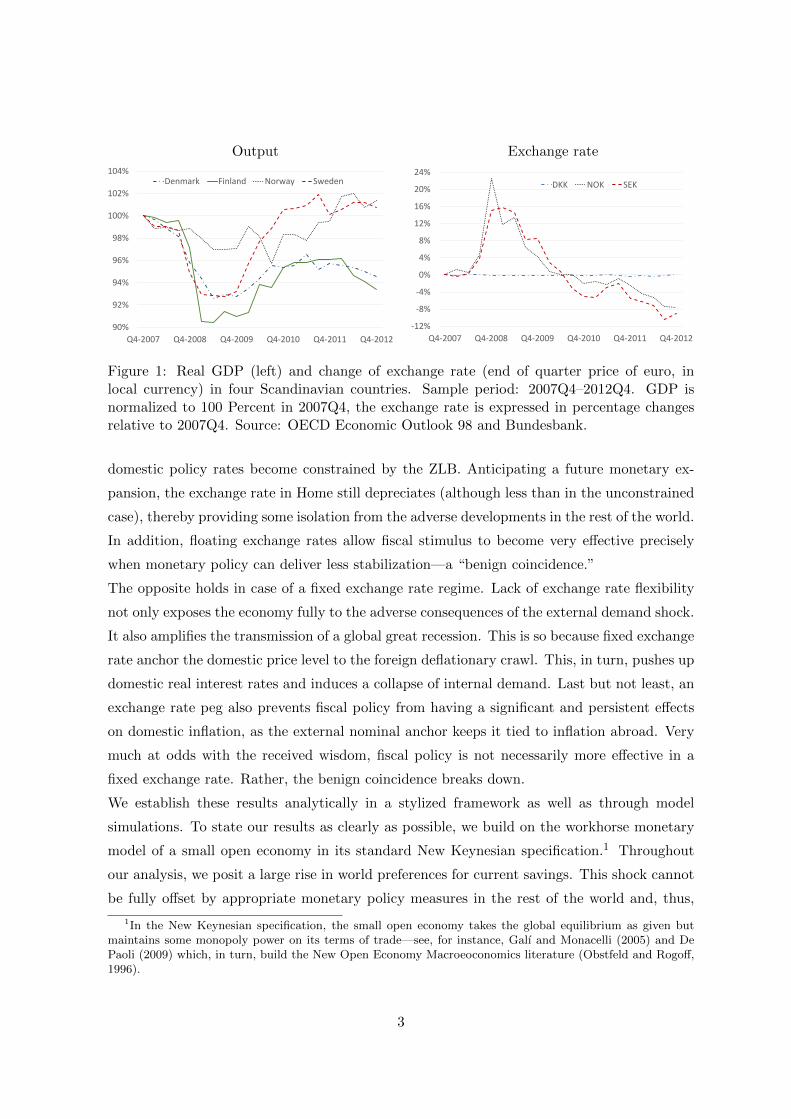
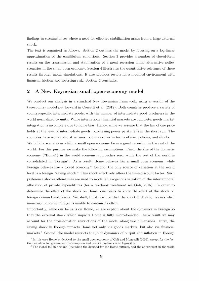
In Figure 2, we look at the transmission of the Foreign saving shock, which causes a sharp

and persistent contraction in Foreign consumption and inflation (not shown). In each panel

vertical axes measure deviations from the pre-shock path, in percent of steady-state output

(in case of quantities) or percent (in case of prices). From the perspective of the small open

12These assumptions imply that the restriction imposed on σ and υ which imposed in our analytical deriva-tions is not satisfied. Yet it turns out that our simulation results are fully in line with our analytical results.This also true for a wide range of alternative values for σ and υ.

17

0 5 10 15-4

-3

-2

-1

0External demand

Float

Peg

ZLB

0 5 10 15-4

-3

-2

-1

0Home output

0 5 10 15-2

-1.5

-1

-0.5

0Inflation

0 5 10 15

-0.6

-0.4

-0.2

0Policy rate

0 5 10 15-6

-4

-2

0Price level

0 5 10 150

2

4

6

Exchange rate

0 5 10 15-2

0

2

4

Terms of trade

0 5 10 15-4

-3

-2

-1

0

Private consumption

0 5 10 15-2

-1.5

-1

-0.5

0

0.5Net exports

Figure 2: Adjustment to one-percent drop of external demand: unconstrained monetarypolicy in Home (dashed line) vs constant-interest-rate period of 10 quarters (solid line) andexchange rate peg (dash-dotted line). Horizontal axes measure time in quarters. Verticalaxes measure deviations from the pre-shock path, in percent of steady state output (in caseof quantities) or percent (in case of prices).

economy, the shock generates a drop of external demand (upper-left panel). In equilibrium,

the shock generates financial inflows corresponding to an external deficit in the trade balance

(depicted in lower-right panel). Contrasting the three scenarios for monetary policy in Home,

we find large differences—notably in terms of the response of domestic output (upper row,

middle panel). Initially, output falls by about four percent under a peg (dash-dotted line),

about two percent if policy rates are fixed for 10 quarters (solid line), and by about one

percent if monetary policy is unconstrained (dashed line).

Several aspects of the transmission mechanism are noteworthy. In case monetary policy is

unconstrained, there is a large upfront cut of interest rates (2nd row, left panel), associated

with a large depreciation of the nominal exchange rate (2nd row, right panel). As a result,

internal demand remains insulated from the full fall-out of the external shock (3rd row,

18

middle panel). In fact, it actually rises at the margin, since a regime of price stability means

that expectations of inflation remain firmly anchored and the long-term real rate, which is

relevant for the consumption decision, falls with the current and anticipated monetary stance.

Despite nominal depreciation and a weakening of the terms of trade (3rd row, left panel), the

contraction in external demand causes a trade deficit. By pursuing price stability, monetary

policy effectively tilts aggregate demand towards domestic consumption.

Exchange rate flexibility plays a crucial role also when monetary policy in Home is con-

strained by the zero lower bound. The economic outlook worsens relative to that under an

unconstrained monetary policy, since insufficient short-term monetary stimulus means that

domestic demand remains inefficiently low. But the depth of the foreign contraction and

deflation translates into a permanent depreciation of Home’s nominal exchange rate. This

weakens the link with the deflationary drift in Foreign: dynamically, the Home price level falls

somewhat (2nd row, middle panel), but not as much as in Foreign (the latter is not shown

in the figure). The terms of trade depreciate, although by less than in case monetary policy

is unconstrained—net exports deteriorate by more. Overall, the contraction in both internal

and external demand causes a fall of domestic output which is about twice as large as in case

monetary policy is unconstrained.

The regime that performs worst, however, is the currency peg. This is because of deflation in

Foreign. If Foreign were not at the ZLB and, hence, would not have suffered a deflationary

drift, a peg would in fact have desirable features. Indeed, to the extent that a credible peg is

an implicit commitment to a stable price level, the transmission of domestic adverse demand

shocks would be muted by the peg. The reason is that any short-run fall in domestic prices

associated with such domestic demand shocks would in the medium or long run be offset

by positive domestic inflation (Cook and Devereux, 2014; Corsetti et al., 2013a). When the

foreign country is at the ZLB and the shock is a demand shock that originates in Foreign,

instead, this conclusion is turned on its head. The implicit domestic commitment that a

pegging country makes to follow the unstable foreign price level works against the country.

Namely, it amplifies the domestic downturn, by generating expectations of sustained domestic

deflation. The terms of trade actually appreciate, exacerbating the contraction of domestic

net exports in response to the shock to foreign demand.

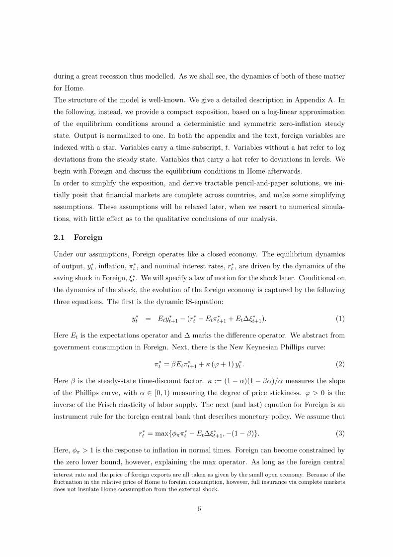
4.2 The scope for fiscal stabilization

Figure 3 traces the effect of an increase of government spending (itself depicted in the upper-

left panel). In the case of a free float, as long as monetary policy is unconstrained, the

fiscal expansion has moderate effects. With the monetary authority ensuring price stability,

19

0 5 10 150

0.5

1Government spending

Float

Peg

ZLB

0 5 10 150

0.5

1

1.5

2Home output

0 5 10 15-0.5

0

0.5

1Inflation

0 5 10 150

0.02

0.04

0.06

0.08Policy rate

0 5 10 150

0.5

1

1.5

2Price level

0 5 10 15-1

0

1

2Exchange rate

0 5 10 15-1

0

1

2Terms of trade

0 5 10 15-0.5

0

0.5

1Private consumption

0 5 10 15-0.4

-0.2

0

0.2

0.4Net exports

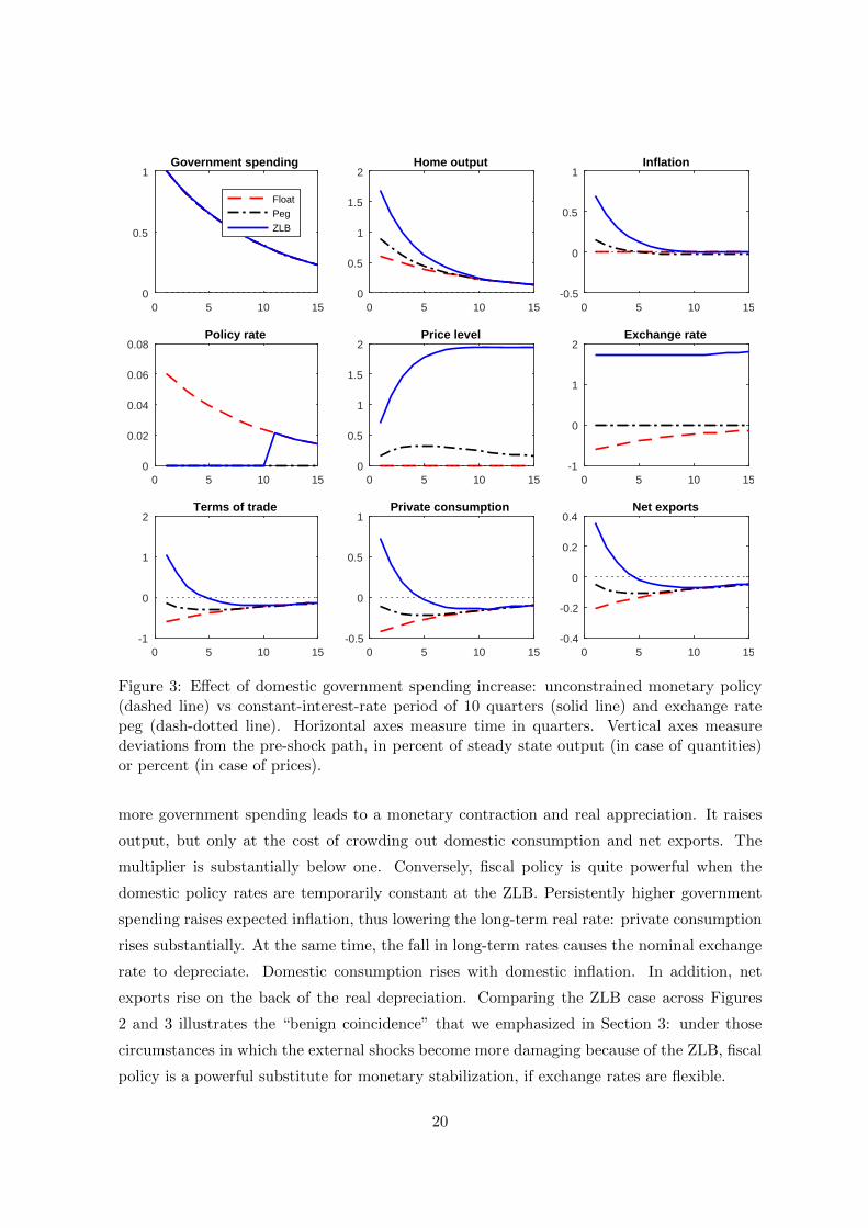
Figure 3: Effect of domestic government spending increase: unconstrained monetary policy(dashed line) vs constant-interest-rate period of 10 quarters (solid line) and exchange ratepeg (dash-dotted line). Horizontal axes measure time in quarters. Vertical axes measuredeviations from the pre-shock path, in percent of steady state output (in case of quantities)or percent (in case of prices).

more government spending leads to a monetary contraction and real appreciation. It raises

output, but only at the cost of crowding out domestic consumption and net exports. The

multiplier is substantially below one. Conversely, fiscal policy is quite powerful when the

domestic policy rates are temporarily constant at the ZLB. Persistently higher government

spending raises expected inflation, thus lowering the long-term real rate: private consumption

rises substantially. At the same time, the fall in long-term rates causes the nominal exchange

rate to depreciate. Domestic consumption rises with domestic inflation. In addition, net

exports rise on the back of the real depreciation. Comparing the ZLB case across Figures

2 and 3 illustrates the “benign coincidence” that we emphasized in Section 3: under those

circumstances in which the external shocks become more damaging because of the ZLB, fiscal

policy is a powerful substitute for monetary stabilization, if exchange rates are flexible.

20

This benign coincidence breaks down, however, when the country pursues a currency peg.

Figure 3 shows that—contrary to conventional wisdom—fiscal policy is not particularly ef-

fective in a fixed exchange rate regime. Note that this is precisely the regime where the

adverse external shock is most consequential for Home output and consumption—compare,

again, Figures 2 and 3. The mechanism governing the transmission of fiscal policy, as dis-

cussed in Corsetti et al. (2013a), is illustrated by the panel in the middle of the figure: by

the working of purchasing power parity in the medium and the long run, under a peg, the

initial positive response of inflation to a government spending expansion will be offset over

time: after a fiscal expansion the price level in Home eventually reverts back to the price level

in Foreign. In the figure here, since Foreign did not receive any shocks, the Home price level

reverts to its pre-shock level. This is in sharp contrast to the evolution of Home prices when

Home monetary policy is constrained by the ZLB but pursues flexible exchange rates. There,

the Home price level keeps increasing over the entire life of the fiscal expansion. Comparing

the two scenarios, therefore, under a peg the overall monetary stance, measured by the rise

in long-term real rates is less rather than more accommodative; and the fiscal multiplier is

correspondingly lower.

4.3 Model extensions: financial frictions and sovereign risk

So far we have proceeded under the assumption of frictionless financial markets, both within

a country and across borders. This assumption is necessary in order to obtain the closed-

form results discussed in the previous section. Here we demonstrate that it is not particularly

consequential for macroeconomic dynamics. In what follows, we perform a sensitivity analysis

and relax the assumption of complete financial markets. We posit that cross-border asset

trade is limited to non-contingent nominal bonds. In addition, we consider the possibility

that Home is vulnerable to a deterioration in the markets’ assessment of sovereign risk.

Drawing on our previous work (Corsetti et al., 2013b, 2014), we assume that sovereign risk in

Home increases when public debt builds up. Higher sovereign risk, in turn, induces a rise of

borrowing costs in the private sector (see also Bocola, forthcoming). This specification entails

that sovereign risk premia result in a contraction of domestic demand and, therefore, a drop

in current economic activity, independently of whether sovereign default actually takes place

or not. We provide some details on the modified model in Appendix A.5. Throughout we

continue to assume that Home is a small open economy.

Using the extended model, we first establish that, under our parameterization, the propaga-

tion of the external-demand shock (the source of this being, as before, a foreign saving shock)

is not fundamentally different if we move from the complete-market economy to an economy

21

0 5 10 15-4

-3

-2

-1

0External demand

Float

Peg

ZLB

0 5 10 15-4

-3

-2

-1

0Home output

0 5 10 15-2

-1.5

-1

-0.5

0Inflation

0 5 10 15

-0.6

-0.4

-0.2

0Policy rate

0 5 10 15-6

-4

-2

0Price level

0 5 10 150

2

4

6

Exchange rate

0 5 10 15-2

0

2

4

Terms of trade

0 5 10 15-4

-3

-2

-1

0

Private consumption

0 5 10 15-2

-1.5

-1

-0.5

0

0.5Net exports

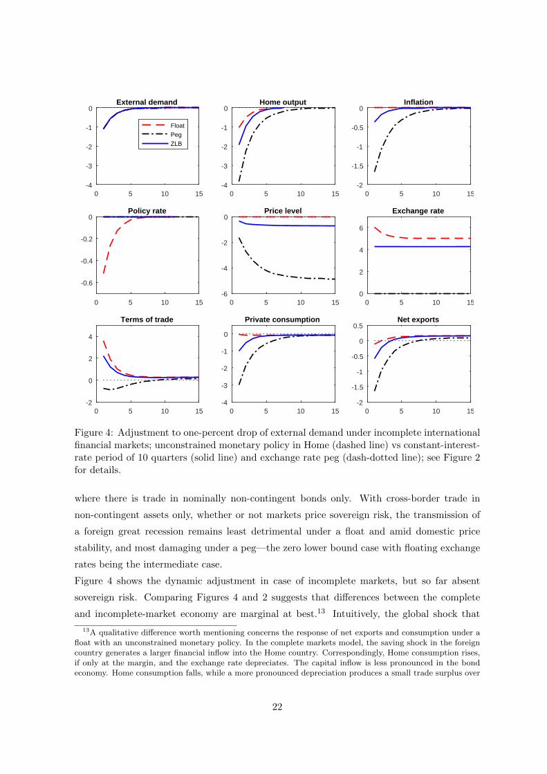
Figure 4: Adjustment to one-percent drop of external demand under incomplete internationalfinancial markets; unconstrained monetary policy in Home (dashed line) vs constant-interest-rate period of 10 quarters (solid line) and exchange rate peg (dash-dotted line); see Figure 2for details.

where there is trade in nominally non-contingent bonds only. With cross-border trade in

non-contingent assets only, whether or not markets price sovereign risk, the transmission of

a foreign great recession remains least detrimental under a float and amid domestic price

stability, and most damaging under a peg—the zero lower bound case with floating exchange

rates being the intermediate case.

Figure 4 shows the dynamic adjustment in case of incomplete markets, but so far absent

sovereign risk. Comparing Figures 4 and 2 suggests that differences between the complete

and incomplete-market economy are marginal at best.13 Intuitively, the global shock that

13A qualitative difference worth mentioning concerns the response of net exports and consumption under afloat with an unconstrained monetary policy. In the complete markets model, the saving shock in the foreigncountry generates a larger financial inflow into the Home country. Correspondingly, Home consumption rises,if only at the margin, and the exchange rate depreciates. The capital inflow is less pronounced in the bondeconomy. Home consumption falls, while a more pronounced depreciation produces a small trade surplus over

22

we place at the core of our analysis is temporary. Self-insurance via intertemporal trade in

bonds and the equilibrium response of the terms of trade and real interest rate at the global

level allow a small open economy to achieve an allocation that is not too far from that with

perfect risk sharing (see, for instance, Cole and Obstfeld, 1991).

Next, we in addition allow for sovereign risk. Including the sovereign risk channel in the

model results in a mild amplification of the adverse effects of the foreign shock. Namely, as

output falls in Home in response to the external shock, government debt builds up due to

the working of automatic stabilizers (that we introduce in the model through a constant tax

rate which is proportional to income). The fiscal outlook worsens, affecting the probability

of default. Markets, in turn, call for a higher sovereign risk premium which impacts private

borrowing conditions in Home adversely. This reduces aggregate demand and activates an

adverse loop: lower demand translates into lower activity, hence higher deficits and debt;

higher debt raises sovereign risk and borrowing costs further.14 Quantitatively, however, the

change in transmission is only moderate. Since the numerical results remain quite similar to

Figure 4, we omit a graph for this case.

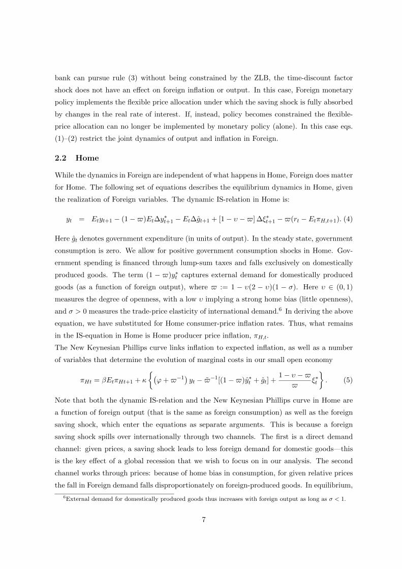
Rather, we emphasize the dimension in which sovereign risk matters a lot, namely, the ef-

fectiveness of fiscal stabilization policy. In this dimension, indeed, the sovereign risk channel

is quite consequential. The effectiveness of fiscal stabilization may be eroded by a loss of

confidence when the government pursues deficit-financed expansions in times of a poor fiscal

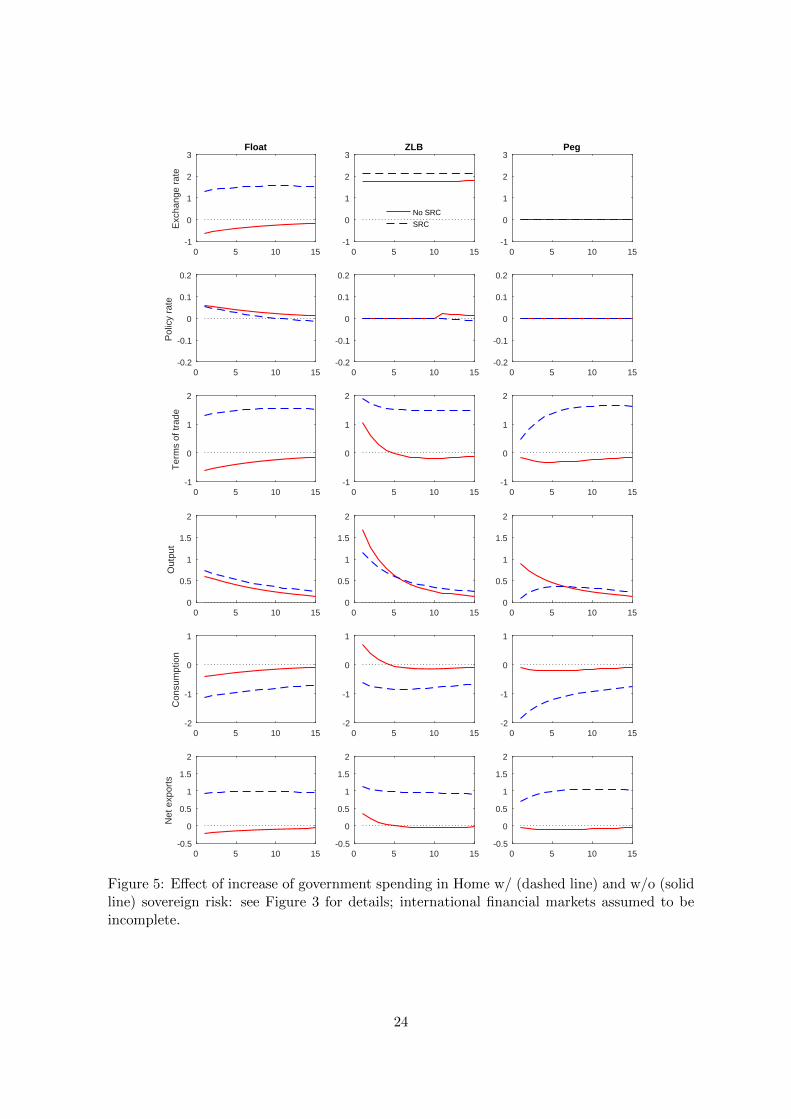
outlook. Figure 5 shows the adjustment to an increase of Home government consumption by

one percent of GDP. The left column shows the responses of the economy under the float

and unconstrained Home monetary policy. The middle column corresponds to a float with

the ZLB constraint binding in Home. The panels on the right show the responses under the

permanent peg. In each of the panels, a solid line marks the responses that would prevail

absent the sovereign risk channel. The dashed line marks the responses with sovereign risk.

Focus on the panels in the fifth row. These show the response of Home consumption. The

columns pertain to the three scenarios for monetary policy. What is very important to note

is that sovereign risk starkly changes the transmission of fiscal policy. In particular, in all

three scenarios, government spending now crowds out domestic demand (see the blue dashed

lines). There is crowding out even at the zero lower bound. Without the sovereign risk

channel, instead, government spending crowded in private consumption (see the solid line in

time.14Under a float and an unconstrained monetary policy, sovereign risk causes more current and/or future

monetary accommodation, reflected by exchange rate depreciation upfront. Although consumption falls, itactually falls by less than in the absence of foreign risk—net exports are correspondingly lower. Monetaryaccommodation and upfront depreciation is instead lower in the ZLB case: the fall in consumption is now morepronounced than in the absence of sovereign risk, making room for a stronger net export dynamic. Under apeg, sovereign risk exacerbates and magnifies the effects under the ZLB scenario.

23

0 5 10 15-1

0

1

2

3

Exc

hang

e ra

te

Float

0 5 10 15-0.2

-0.1

0

0.1

0.2

Pol

icy

rate

0 5 10 15-1

0

1

2

Ter

ms

of tr

ade

0 5 10 150

0.5

1

1.5

2

Out

put

0 5 10 15-2

-1

0

1

Con

sum

ptio

n

0 5 10 15-0.5

0

0.5

1

1.5

2

Net

exp

orts

0 5 10 15-1

0

1

2

3ZLB

No SRC

SRC

0 5 10 15-0.2

-0.1

0

0.1

0.2

0 5 10 15-1

0

1

2

0 5 10 150

0.5

1

1.5

2

0 5 10 15-2

-1

0

1

0 5 10 15-0.5

0

0.5

1

1.5

2

0 5 10 15-1

0

1

2

3Peg

0 5 10 15-0.2

-0.1

0

0.1

0.2

0 5 10 15-1

0

1

2

0 5 10 150

0.5

1

1.5

2

0 5 10 15-2

-1

0

1

0 5 10 15-0.5

0

0.5

1

1.5

2

Figure 5: Effect of increase of government spending in Home w/ (dashed line) and w/o (solidline) sovereign risk: see Figure 3 for details; international financial markets assumed to beincomplete.

24

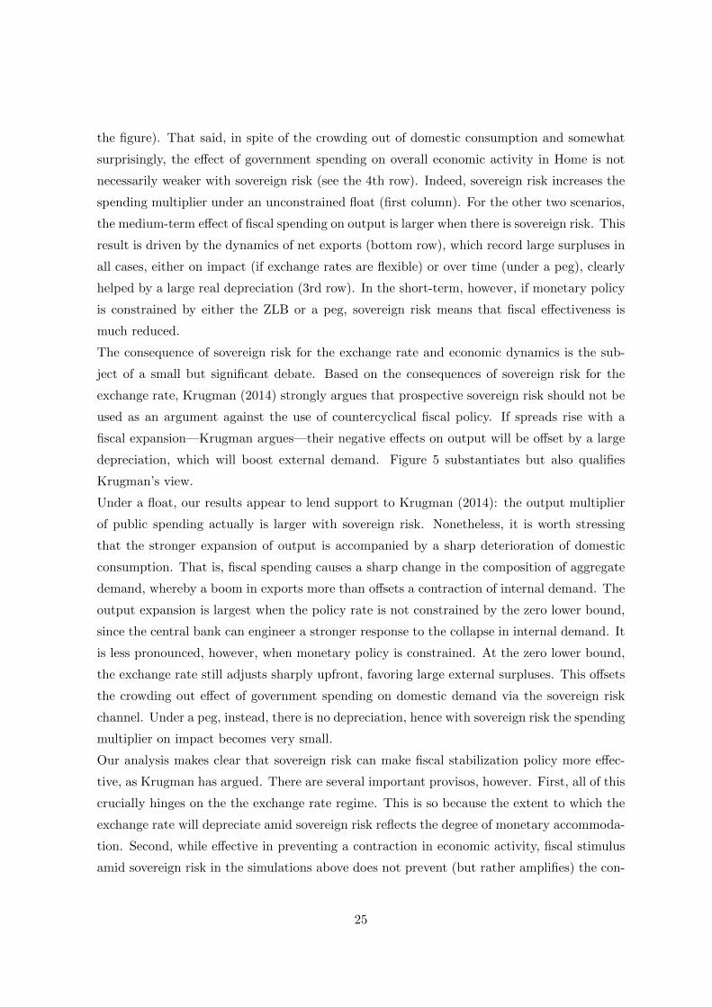
the figure). That said, in spite of the crowding out of domestic consumption and somewhat

surprisingly, the effect of government spending on overall economic activity in Home is not

necessarily weaker with sovereign risk (see the 4th row). Indeed, sovereign risk increases the

spending multiplier under an unconstrained float (first column). For the other two scenarios,

the medium-term effect of fiscal spending on output is larger when there is sovereign risk. This

result is driven by the dynamics of net exports (bottom row), which record large surpluses in

all cases, either on impact (if exchange rates are flexible) or over time (under a peg), clearly

helped by a large real depreciation (3rd row). In the short-term, however, if monetary policy

is constrained by either the ZLB or a peg, sovereign risk means that fiscal effectiveness is

much reduced.

The consequence of sovereign risk for the exchange rate and economic dynamics is the sub-

ject of a small but significant debate. Based on the consequences of sovereign risk for the

exchange rate, Krugman (2014) strongly argues that prospective sovereign risk should not be

used as an argument against the use of countercyclical fiscal policy. If spreads rise with a

fiscal expansion—Krugman argues—their negative effects on output will be offset by a large

depreciation, which will boost external demand. Figure 5 substantiates but also qualifies

Krugman’s view.

Under a float, our results appear to lend support to Krugman (2014): the output multiplier

of public spending actually is larger with sovereign risk. Nonetheless, it is worth stressing

that the stronger expansion of output is accompanied by a sharp deterioration of domestic

consumption. That is, fiscal spending causes a sharp change in the composition of aggregate

demand, whereby a boom in exports more than offsets a contraction of internal demand. The

output expansion is largest when the policy rate is not constrained by the zero lower bound,

since the central bank can engineer a stronger response to the collapse in internal demand. It

is less pronounced, however, when monetary policy is constrained. At the zero lower bound,

the exchange rate still adjusts sharply upfront, favoring large external surpluses. This offsets

the crowding out effect of government spending on domestic demand via the sovereign risk

channel. Under a peg, instead, there is no depreciation, hence with sovereign risk the spending

multiplier on impact becomes very small.

Our analysis makes clear that sovereign risk can make fiscal stabilization policy more effec-

tive, as Krugman has argued. There are several important provisos, however. First, all of this

crucially hinges on the the exchange rate regime. This is so because the extent to which the

exchange rate will depreciate amid sovereign risk reflects the degree of monetary accommoda-

tion. Second, while effective in preventing a contraction in economic activity, fiscal stimulus

amid sovereign risk in the simulations above does not prevent (but rather amplifies) the con-

25

traction in internal demand. Our reading of this is that, in light of the above, and especially

given the limits of our understanding of financial and fiscal crises, the arguments for dynamic

budget correction and policies maintaining a stable fiscal outlook remain strong.15

In the previous section, we have entertained the notion that the stabilization of large external

shocks under flexible exchange rates may benefit from a “benign coincidence”, with fiscal

policy becoming becomes most effective at stabilizing domestic activity when the external

shock is most detrimental. Earlier, we already qualified that the benign coincidence holds

only under flexible exchange rates. The analysis above, qualifies this further. The benign

coincidence does not only require floating exchange rates, it also applies reliably only when

sovereign risk is not an important consideration.

5 Conclusion

The global economy remains vulnerable. In particular, there is a risk that large global shocks

once cause again the world economy to fall into a great recession. This is a challenge to

policymaking in small open economies, which by their very openness to trade are particularly

vulnerable to external shocks. In this paper we provide a stylized analysis of the effectiveness

of different monetary and fiscal policies in a small open economy that is faces a large external

demand shock. Specifcally, we model a shock to the rest of the world’s desire to save that

occurs at a time when policy rates in the rest of the world are constrained, for example,

due to the zero lower bound. The shock causes world aggregate demand to fall and a global

deflationary crawl. We reassess the effect that fiscal and monetary policies (in particular, the

exchange rate regime) have on the evolution of the small open economy in the wake of the

shock. We explicitly account for potential constraints on either policy, in the form of a zero

lower bound constraint on domestic monetary policy or an exchange-rate peg, or concerns

with sovereign risk which may constrain fiscal policy.

We analyze in detail the specific way in which a flexible exchange rate can act as a shock

absorber under circumstances which have been defining features of the great recession and

which may re-occur in the near future. A central result of our analysis is that for the exchange

rate to isolate the small open economy from the external shock, it needs to decouple domestic

inflation from the deflationary crawl that afflicts the world economy. This requires Home

policymakers to manage a depreciation drift in the nominal exchange rate, over and above

the nominal and real depreciation needed to buffer the Home economy from the collapse in

15The strong response of net exports to a government-spending expansion is also noteworthy in light ofthe ongoing controversy on currency wars. Our model suggests that, in a sovereign risk crisis, even fiscalstabilization—typically targeted to sustain internal demand—tends to increase net saving in the economy, andrequire currency depreciation to be effective.

26

external demand alone.

If monetary policy cannot manage that drift, fiscal policy—in principle—can be used to

stabilize the small open economy. However, we find that fiscal policy will be an effective

tool only when the monetary regime that is such that it can accompany fiscal stimulus with

enough monetary accommodation, and an exchange rate regime that insulates the evolution

of the domestic price level from the price level abroad. If that is the case, fiscal policy turns

out to be particularly effective when the effect of the external shock is largest, namely, when

domestic monetary policy is temporarily constrained by the zero lower bound. The same does

not hold under an exchange rate peg.

Modern monetary theory indeed questions the conventional wisdom from the textbook ren-

dition of the Mundell-Fleming model, that fiscal policy is a reliable alternative to monetary

policy in a currency peg or a monetary union. Furthermore we find that the conventional

Mundell-Fleming logic is particularly misleading if there is a loss of confidence in the sovereign

debt market that risks affecting the domestic private sector’s financial conditions. Indeed,

whether sovereign risk reduces the effectiveness of spending stimulus greatly depends on the

monetary regime as well. Sovereign risk greatly reduces the effectiveness of spending stimulus

if the small open economy is subject to a pegged exchange rate, and to a lesser extent if it

is subject to the zero lower bound. The opposite is true when the small open economy has

opted for floating exchange rates and its monetary policy is not constrained.

In sum, we find that the risk of another great recession strengthens the case for flexible

exchange rates.

References

Benigno, Gianluca, Pierpaolo Benigno, and Fabio Ghironi (2007). “Interest rate rules for fixed

exchange rate regimes”. Journal of Economic Dynamics and Control 31 (7), 2196–2211.

Berkmen, S. Pelin, Gaston Gelos, Robert Rennhack, and James P. Walsh (2012). “The global

financial crisis: Explaining cross-country differences in the output impact”. Journal of

International Money and Finance 31 (1), 42–59.

Bocola, Luigi (forthcoming). “The Pass-Through of Sovereign Risk”. Journal of Political

Economy.

Christiano, Lawrence, Martin Eichenbaum, and Sergio Rebelo (2011). “When is the govern-

ment spending multiplier large?” Journal of Political Economy 119 (1), 78 –121.

Clarida, Richard, Jordi Gali, and Mark Gertler (2001). “Optimal Monetary Policy in Open

versus Closed Economies: An Integrated Approach”. American Economic Review 91 (2),

248–252.

27

Cole, Harold L. and Maurice Obstfeld (1991). “Commodity trade and international risk shar-

ing : How much do financial markets matter?” Journal of Monetary Economics 28 (1),

3–24.

Cook, David and Michael B. Devereux (2011). “Optimal fiscal policy in a world liquidity

trap”. European Economic Review 55 (4), 443–462.

(2013). “Sharing the Burden: Monetary and Fiscal Responses to a World Liquidity

Trap”. American Economic Journal: Macroeconomics 5 (3), 190–228.

(2014). “Exchange rate flexibility under the zero lower bound”. Globalization and

Monetary Policy Institute Working Paper 198. Federal Reserve Bank of Dallas.

Corsetti, Giancarlo, Andre Meier, and Gernot J. Muller (2012). “What determines government

spending multipliers?” Economic Policy 27 (72), 521–565.

Corsetti, Giancarlo, Keith Kuester, and Gernot J. Muller (2013a). “Floats, Pegs and the

Transmission of Fiscal Policy”. Fiscal Policy and Macroeconomic Performance. Ed. by

Luis Felipe Cespedes and Jordi Gali. Vol. 17. Central Banking, Analysis, and Economic

Policies Book Series. Central Bank of Chile. Chap. 7, 235–281.

Corsetti, Giancarlo, Keith Kuester, Andre Meier, and Gernot J. Muller (2013b). “Sovereign

risk, fiscal policy, and macroeconomic stability”. Economic Journal 123 (566), F99–F132.

Corsetti, Giancarlo, Keith Kuester, Andre Meier, and Gernot J Muller (2014). “Sovereign

risk and belief-driven fluctuations in the euro area”. Journal of Monetary Economics 61,

53–73.

Curdia, Vasco and Michael Woodford (2009). “Credit frictions and optimal monetary policy”.

BIS Working Papers 278. Bank for International Settlements.

De Paoli, Bianca (2009). “Monetary policy and welfare in a small open economy”. Journal of

International Economics 77, 11–22.

Erceg, Christopher J. and Jesper Linde (2012). “Fiscal Consolidation in an Open Economy”.

American Economic Review 102 (3), 186–91.

Farhi, Emmanuel and Ivan Werning (2012). “Fiscal Multipliers: Liquidity Traps and Currency

Unions”. NBER Working Papers 18381. National Bureau of Economic Research.

Friedman, Milton (1953). “The case for flexible exchange rates”. In: essays in positive eco-

nomics. University of Chicago Press, 157–203.

Galı, Jordi (2015). Monetary policy, inflation and the business cycle: an introduction to the

new keynesian framework. 2nd ed. Princeton University Press.

Galı, Jordi and Tommaso Monacelli (2005). “Monetary policy and exchange rate volatility in

a small open economy”. Review of Economic Studies 72, 707–734.

Kriwoluzky, Alexander, Martin Wolf, and Gernot J. Muller (2015). “Exit expectations and

debt crises in currency unions”.

Krugman, Paul (2014). “Currency Regimes, Capital Flows, and Crises”. IMF Economic Re-

view 62 (4), 470–493.

28

Obstfeld, Maurice and Kenneth S. Rogoff (1996). Foundations of International Macroeco-

nomics. Vol. 1. MIT Press Books 0262150476. The MIT Press.

Schmitt-Grohe, Stephanie and Martin Uribe (2003). “Closing small open economy models”.

Journal of International Economics 61 (1), 163–185.

Schmitt-Grohe, Stephanie and Martın Uribe (2015). “Downward Nominal Wage Rigidity, Cur-

rency Pegs, and Involuntary Unemployment”. Journal of Political Economy, forthcoming.

Sutherland, Alan (2005). “Incomplete pass-through and the welfare effects of exchange rate

variability”. Journal of International Economics 65 (2), 375–399.

Woodford, Michael (2011). “Simple analytics of the government expenditure multiplier”.

American Economic Journal: Macroeconomics 3 (1), 1–35.

29

A A New Keynesian open-economy model

Our model is a simplified version of the two-country model put forward in Corsetti et al.

(2012), as we abstract from investment and wage rigidities. Home trades with the rest of the

world, consolidated in a Foreign country. Both countries produce a variety of country-specific

intermediate goods, with the number of intermediate good producers normalized to unity.

A fraction n of firms is located in Home, the remaining firms (n, 1] are located in Foreign.

Analogously, Home accounts for a fraction n ∈ [0, 1] of the global population. Intermediate

goods are traded across borders while final goods which are bundles of intermediate goods, are

not. Prices of intermediate goods are sticky in producer-currency terms. Households supply

labor services only within the country where they reside, but trade assets internationally. For

the sake of analytical tractability, in our baseline, they will trade a complete set of state-

contingent assets.

Many of the features of the model are standard, so we keep the exposition short. We focus our

exposition on Home. When necessary, we refer to foreign variables by means of an asterisk.

A.1 Households

There is a representative household in each country. Letting Ct denote a consumption basket

(defined below) and Ht labor supply, the objective of the household is

maxEt

∞∑k=0

(eξt+kβk)

(lnCt+k −

H1+ϕt+k

1 + ϕ

), (25)

where ξt is a zero-mean shock to the time-discount factor, β ∈ (0, 1) is the discount factor,

and ϕ > 0 is the inverse of the Frisch elasticity of labor supply.

In our baseline, the household trades a complete set of state-contingent securities with the

rest of the world. Letting Xt+1 denote the payoff in units of domestic currency in period t+ 1

of the portfolio held at the end of period t, the budget constraint of the household is given by

Et {ρt,t+1Xt+1} − Xt = (1− τ)(WtHt + Υt)− Tt − PtCt.

Here ρt,t+1 is the nominal stochastic discount factor. Wt is the nominal wage. Υt are the

domestic firms’ nominal profits. τ is a constant tax rate, Tt are lump-sum taxes. Pt is the

price index for the final consumption basket. The consumption baskets themselves are not

traded across borders. Their components are, however. The baskets consist of bundles At

and Bt of, respectively, domestically and foreign produced intermediate goods. The final

30

consumption basket Ct (C∗t ) is produced using the following aggregation technology

Ct =

{[(1− (1− n)υ)]

1σ A

σ−1σ

t + [(1− n)υ)]1σ B

σ−1σ

t

} σσ−1

, (26)

C∗t ={

[nυ]1σ (A∗t )

σ−1σ + [(1− nυ)]

1σ (B∗t )

σ−1σ

} σσ−1

, (27)

where σ measures the terms of trade elasticity of the relative demand for domestically pro-

duced goods and υ ∈ [0, 1] measures the home bias.16

The bundles of domestically and imported intermediate goods are defined as follows

At =

[(1

n

) 1ε∫ n

0At(j)

ε−1ε dj

] εε−1

, Bt =

[(1

1− n

) 1ε∫ 1

nBt(j)

ε−1ε dj

] εε−1

, (28)

where At(j) and Bt(j) denote intermediate goods produced in Home and Foreign, respectively,

and ε measures the elasticity of substitution between intermediate goods produced within the

same country.

The household minimizes expenditures subject to (26) and (28). Specifically, let Pt(j) denote

the price of an intermediate good expressed in domestic currency and Et the nominal exchange

rate (the price of foreign currency in terms of domestic currency). We assume that the law

of one price holds, so that

EtP ∗t (j) = Pt(j). (29)

The household’s expenditure minimization implicitly defines a demand function for intermedi-

ate goods. Assuming that government consumption, Gt, is a bundle isomorphic to final goods,

but consisting of domestically produced goods only, global demand for a generic intermediate

good produced in Home and Foreign is, respectively:

Y Dt (j) =

(Pt(j)

PHt

)−ε{(PHtPt

)−σ [ (1− (1− n)υ)Ct

+(1− n)υQσt C∗t

]+Gt

}, (30)

Y Dt (j)∗ =

(P ∗t (j)

P ∗Ft

)−ε{(P ∗FtP ∗t

)−σ [nυQ−σt Ct + (1− nυ)C∗t

]}, (31)

where price indices are given by

PHt =

[1

n

∫ n

0Pt(j)

1−εdj

] 11−ε

, PFt =

[1

1− n

∫ 1

nPt(j)

1−εdj

] 11−ε

, (32)

16This specification follows Sutherland (2005) and De Paoli (2009). With υ = 1, there is no home bias: if therelative price of foreign and domestic goods is unity, the fraction of domestically produced goods which endsup in the production of final goods is equal to n, while imports account for a share of 1−n. Importantly, finalgoods are identical across countries in this case. A lower value of υ implies that the fraction of domesticallyproduced goods in final goods exceeds the share of domestic production in the world economy. If υ = 0, thereis full home bias and no trade across countries.

31

Pt =[(1− (1− n)υ)P 1−σ

Ht + ((1− n)υ)P 1−σFt

] 11−σ , (33)

P ∗t =[nυ (P ∗Ht)

1−σ + (1− nυ) (P ∗Ft)1−σ] 1

1−σ, (34)

and

Qt =EtP ∗tPt

(35)

measures the real exchange rate.

A.2 Firms

Intermediate good producers sell under monopolistic competition, facing the demand function

(30). The production function is Cobb-Douglas:

Yt(j) = Ht(j) (36)

where Ht(j) denotes labor services employed by firm j ∈ [0, n] in period t.

We assume that prices are set in the currency of the producer and that price setting is

constrained exogenously a la Calvo, so that in each period only a fraction of intermediate

good producers (1− α) may adjust its price. When firm j has the opportunity, it sets Pt(j)

to maximize the expected discounted value of net profits:

maxPt(j)

∞∑k=0

αt+kEtρt,t+k

{Pt(j)Y

Dt+k(j)−Ψ

[Y Dt+k(j)

]}subject to the demand function (30) and the production function (36); Ψ

[Y Dt+k(j)

]mea-

sures costs. Domestic households own the firms, so profits are discounted with the domestic

households’ stochastic discount factor.

A.3 Monetary and fiscal policy

We assume that monetary policy is conducted by adjusting the short-term nominal interest

rate:

Rt ≡ 1/Etρt,t+1.

As regards fiscal and budget policy, we assume that Home government spending falls on an

aggregate of domestic intermediate goods only. We also posit that intermediate goods are

assembled so as to minimize costs. Thus the price index for government spending is given by

PH,t. In the first part of the paper, without loss of generality, we assume that the government

budget is balanced in each period by means of lump-sum taxes Tt. In the second part of the

paper, we will consider a richer specification, so as to account for the possibility of sovereign

risk.

32

A.4 Equilibrium

In equilibrium, firms and households optimally choose prices and quantities subject to their

respective constraints and initial conditions while markets clear. At the level of inter-

mediate goods we have Yt(j) = Yt(j)D. Defining an index for aggregate output Yt =(∫ 1

0 Yε−1ε

t (j)dj

) εε−1

, we obtain

Yt =

(PHtPt

)−σ[(1− (1− n)υ)Ct + (1− n)υQσt C

∗t ] +Gt. (37)

Labor markets clear if

Ht =

∫ n

0Ht(j)dj (38)

Finally, asset markets clear by Walras’ law.

In our analysis we focus on the limiting case n→ 0 for the size of the domestic economy:

Yt =(PHtPt

)−σ[(1− υ)Ct + υQσt C

∗t ] +Gt,

Y ∗t = C∗t .

This makes the Home economy de facto a small open economy. Foreign, instead, operates

like a closed economy. But – importantly – it may be a source of shocks for Home.

A.5 Incomplete financial markets

We also consider a variant of the model where financial markets are incomplete. Specifically, in

the modified model, we restrict asset trade to nominally non-contingent bonds only. Moreover,

we relax the assumption that government debt is neutral and allow it to impact the economy

through the sovereign risk channel. Denote with Dt the stock of nominal debt issued by the

fiscal authorities, assumed to have a maturity of one period. The period budget constraint of

the government reads as follows:

QD,tDt = Dt−1[1− δI(default in t+ 1)] +Gt − τYt − Tt, (39)

where δ > 0 is the fixed haircut that the government applies to private holders of its own

debt in those states of the world in which it defaults. I(default in t + 1) is the indicator

function that takes a value of one in case the government defaults and is zero otherwise. As

in Corsetti et al. (2013b), the probability of default in period t, pt, may increase in the level

of debt relative to steady-state output according to the following random function:

pt = Fbeta

(Dt

4Y

1

d;αbg , βbg

). (40)

33

Here d denotes the upper end of the support for the debt-to-GDP ratio and Fbeta marks the

CDF of the beta distribution. That is, from an ex ante perspective, the government applies

the haircut δ in the next period with probability pt+1. With the opposite probability, the

government will comply with its promises to pay.

Finally, we postulate that lump-sum taxes adjust to stabilize debt in the following way:

Tt = φdDt, with φd > 1− β.

Households trade two discount bonds on international financial markets, one paying one unit

of domestic currency in the next period, the other one unit of foreign currency. Specifically,

letting Bt denote the domestic-currency bond and B∗t the foreign-currency bond, traded at

price QB,t and QB∗,t, respectively, the budget constraint of a household in Home reads as

follows

QB,tBt +QB∗,tB∗t Et + PtCt = (1− τ)Yt − Tt +Bt−1 +B∗t−1Et, (41)

where τ is a constant tax rate.

For tractability, we assume that sovereign default is possible only in the Home country and

that the marginal investor in sovereign bonds is a small mass of risk-neutral investors in

Foreign. Since Home bonds are subject to both outright sovereign default (a haircut), and

the risk of changes in the price of currencies, the bond price schedule is

QD,t = βEt {[1− δI(default in t+ 1)] Et/Et+1} . (42)

Sovereign default risk in the Home country, in turn, is assumed to spill over to private-sector

bond prices as follows

QB,t = R−1t Et[1− ηδI(default in t+ 1)], QB∗,t = βEt[1− ηδI(default in t+ 1]. (43)

where the parameter η ≥ 0 captures the degree of spillover of sovereign risk into private

borrowing. Following Corsetti et al. (2013b) we rationalize a value of η larger than zero

by the observation that private-sector contracts may not be fully enforced in the event of a

sovereign default.17 Importantly, however, we assume that even though lenders may not be

fully serviced in the event of sovereign default, borrowers may not retain resources either.

Rather, resources are lost in the process.18

We reconsider our earlier experiments in our modified model, based on simulations through-

out. For this purpose we rely on a first order approximation to the equilibrium conditions

17Specification (43) follows Kriwoluzky et al. (2015).18Hence, whether the sovereign defaults or not has no direct bearing on the household’s budget constraint.

Otherwise, borrowers’ interest rate would rise with sovereign risk only notionally, not affecting behaviour upto first order, as explained in Curdia and Woodford (2009). Bocola (forthcoming) models the pass-through ofsovereign risk while explicitly accounting for financial intermediation.

34

around a deterministic steady state. As before, there is no debt and inflation in steady state.

The strength of the sovereign risk channel is captured by three parameters: the sensitivity of

Fbeta to the debt level (how steeply the default risk rises in debt), the size of the haircut in the

event of default, δ, and the spillover parameter η. Eventually, our assumptions imply that an

increase of sovereign debt by one percent of GDP, raises the interest rates faced by the private

sector by half a basis point. This corresponds to a scenario of severe fiscal stress, according

to our earlier work (Corsetti et al., 2013b). We ensure stationarity by assuming that the

private-sector interest rate is also elastic in the net foreign asset position of the private sector

(Schmitt-Grohe and Uribe, 2003).

B System of linear difference equations

A linear approximation to the equilibrium conditions of the complete markets model yields

the following system of expectational difference equations. Small letters indicate the log

deviation of a variable from its steady-sate value. We first focus on the baseline model

allowing for n ∈ [0, 1].

B.1 Baseline

Households supply labor according to

wt = ϕht + ct +τ

1− ττt (B.1)

w∗t = ϕh∗t + c∗t +τ

1− ττ∗t , (B.2)

where wt is the (consumption) real wage. The optimal time path of consumption satisfies:

ct = Et(ct+1)− (it − Etπt+1) (B.3)

c∗t − ξ∗t = Et(c∗t+1 − ξ∗t+1)− (i∗t − Etπ∗t+1). (B.4)

Under complete financial markets, we have the following risk-sharing condition:

(ct − ξt)− (c∗t − ξ∗t ) = qt = (1− υ)st. (B.5)

Intermediate good firms’ price-setting behavior is given by

πAt = βEtπAt+1 + κmct (B.6)

π∗Bt = βEtπ∗Bt+1 + κmc∗t , (B.7)

35

where marginal costs are given by

mct = wt − qH,t (B.8)

mc∗t = w∗t − q∗F,t. (B.9)

The aggregate production function is given by

yt = ht (B.10)

y∗t = h∗t . (B.11)

Relative prices satisfy

πHt = qHt − qHt−1 + πt (B.12)

π∗Ft = q∗Ft − q∗Ft−1 + π∗t , (B.13)

as well as

−qt + qHt = q∗Ht (B.14)

−qt + qFt = q∗Ft. (B.15)

From the definition of the real exchange rate we have

qFt − qFt−1 = det + π∗t − πt + q∗Ft − q∗Ft−1. (B.16)

Deflated price indices

0 = (1− (1− n)ω)qHt + (1− n)ωqFt (B.17)

0 = (1− nω)q∗Ft + nωq∗Ht. (B.18)

Finally, there is market clearing:

yt =(1− n)υ(cyc∗t + σcyqt)− σcyqHt + (1− (1− n)υ)cyct + (1− cy)gt (B.19)

y∗t =nυ(ct − σqt)− σq∗Ft + (1− nυ)c∗t . (B.20)

B.2 Incomplete markets model

The incomplete markets model assumes n → 0, that is, Home is small. Instead of the risk-

sharing condition B.5, equilibrium require the following UIP condition to hold:

rt − r∗t = Etet+1 − et.

36

Also, we need to keep track private-sector bond holds. Assuming that foreign-currency bonds

are in zero net supply we have:

βbt + ct = bt−1 + (1− τ)yt − ct − cyqH,t − tt. (B.21)

(B.22)

If the sovereign risk-channel is operative, we need to keep track of government debt:

βdrt+1 = drt + gt − trt − τyt (B.23)

tt = ψddt. (B.24)

Here the second equation determines the adjustment of taxes to debt. Eventually, the

sovereign risk channel alters the Euler equation in Home

ct = Etct+1 − (it − Etπt+1 + χdt + γbt),

where χ captures the pass-through of sovereign risk (which rises in public debt) into private

borrowing conditions; γ makes the effective interest rate dependent on the net foreign asset

position.

37