The Cauchy problem for nonlocal evolutionequations

Alex Himonas

Department of Mathematics

Mini-workshop non-local dispersive equations

NTNU, Trondheim, Norway

September 21–23, 2015

Abstract

We shall consider the initial value problem for nonlocal and nonlinearevolution equations having peakon traveling wave solutions anddiscuss their well-posedness in Sobolev and analytic spaces. Theseinclude the Camassa-Holm (CH), the Degasperis-Procesi (DP), theNovikov (NE), and the Fokas-Olver-Rosenau-Qiao (FORQ) equations,which are integrable. Also, for these equations we shall discussstability properties of the data-to-solution map. The talk is based onwork with Carlos Kenig, Gerard Misio lek, Gustavo Ponce, CurtisHolliman, Dionyssis Mantzavinos, Gerson Petronilho and RafaelBarostichi.

Historical remarks

• 1973: G. B. Whitham, “Linear and Nonlinear waves, p. 476”

13.14 Breaking and Peaking

“It was remarked earlier that the nonlinear shallow waterequations which neglect dispersion altogether lead to breaking ofthe typical hyperbolic kind, with the development of a verticalslope and a multivalued profile. It seems clear that the thirdderivative term in the Korteweg-deVries equation will prevent thisever happening in its solutions.

. . .

Although both breaking and peaking, as well as criteria for theoccurrence of each, are without doubt contained in the equationsof the exact potential theory, it is intriguing to know whatkind of simpler mathematical equation could include allthese phenomena.”

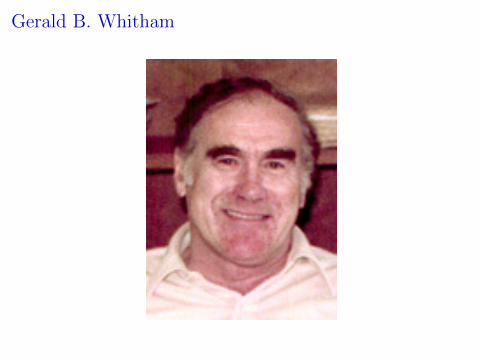
Gerald B. Whitham

Historical remarks (cont.)Witham in this book continues by proposing a KdV-type equationwith a weaker dispersion for modeling (hopefully) “breaking andpeaking” shallow water waves. This equation is of the form:

ut +(N(u) + L(u)

)x

= 0 (1)

where

· N = nonlinearity· L = linear “weak” dispersion

KdV(order of dispersion =3): ChoosingN(u) = 1

2u2, L(u) = 1 + 1

6∂2x =⇒

ut + uux + ux +1

6∂3xu = 0. (KdV ) (2)

Whitham Equation(order of dispersion =1/2): Choosing

N(u) =1

2u2, Lf(ξ) =

( tanh ξ

ξ

)1/2f(ξ) ≈ |ξ|−1/2f(ξ) =⇒

ut + uux + ∂xLu = 0. (WE) (3)

u(x, t) =c

2sech2

(√c

2(x− ct)

), u(x, t) = ce−|x−ct|

Figure: KdV soliton & peaked soliton

KdV story

• 1834: Scott Russell reported his “large wave of translation”,nowadays known as soliton, that he observed in the Edinburghchannel while following a barge on horseback.

• 1877: Boussinesq, in his attempt to explain the soliton, derivedapproximations to the Navier-Stokes equations in severaldifferent regimes, among which the so-called KdV equation

ut + ux + uux + uxxx = 0.

• 1895: Korteweg and de Vries rederived the KdV.

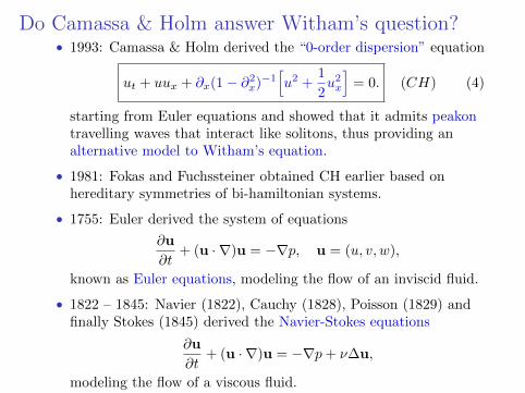
Do Camassa & Holm answer Witham’s question?• 1993: Camassa & Holm derived the “0-order dispersion” equation

ut + uux + ∂x(1− ∂2x)−1[u2 +

1

2u2x

]= 0. (CH) (4)

starting from Euler equations and showed that it admits peakontravelling waves that interact like solitons, thus providing analternative model to Witham’s equation.

• 1981: Fokas and Fuchssteiner obtained CH earlier based onhereditary symmetries of bi-hamiltonian systems.

• 1755: Euler derived the system of equations

∂u

∂t+ (u · ∇)u = −∇p, u = (u, v, w),

known as Euler equations, modeling the flow of an inviscid fluid.

• 1822 – 1845: Navier (1822), Cauchy (1828), Poisson (1829) andfinally Stokes (1845) derived the Navier-Stokes equations

∂u

∂t+ (u · ∇)u = −∇p+ ν∆u,

modeling the flow of a viscous fluid.

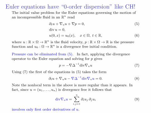
Euler equations have “0-order dispersion” like CH!The initial value problem for the Euler equations governing the motion ofan incompressible fluid in an Rn read

∂tu +∇uu +∇p = 0, (5)

div u = 0,

u(0, x) = u0(x), x ∈ Ω, t ∈ R, (6)

where u : R× Ω→ Rn is the fluid velocity, p : R× Ω→ R is the pressurefunction and u0 : Ω→ Rn is a divergence free initial condition.

Pressure can be eliminated from (5). In fact, applying the divergenceoperator to the Euler equation and solving for p gives

p = −∇∆−1div∇uu (7)

Using (7) the first of the equations in (5) takes the form

∂tu +∇uu−∇∆−1div∇uu = 0. (8)

Note the nonlocal term in the above is more regular than it appears. Infact, since u = (u1, . . . , un) is divergence free it follows that

div∇uu =n∑

i,j=1

∂iuj ∂jui (9)

involves only first order derivatives of u.

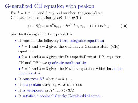
Generalized CH equation with peakonFor k = 1, 2, · · · and b any real number, the generalizedCamassa-Holm equation (g-kbCH or gCH)

(1− ∂2x)ut = ukuxxx + buk−1uxuxx − (b+ 1)ukux. (10)

has the fllowing important properties:

• It contains the following three integrable equations:

• k = 1 and b = 2 gives the well known Camassa-Holm (CH)equation.

• k = 1 and b = 3 gives the Degasperis-Procesi (DP) equation.

CH and DP have quadratic nonlinearities.

• k = 2 and b = 3 gives the Novikov equation, which has cubicnonlinearities.

• It conserves H1 when b = k + 1.

• It has peakon traveling wave solutions.

• It is well-posed in Hs for s > 3/2

• It satisfies a nonlocal Cauchy-Kovalevski theorem.

Integrable equations

Integrable equations possess many special properties including:

• an infinite hierarchy of higher symmetries,

• infinitely many conserved quantities,

• a Lax pair,

• a bi-Hamiltonian formulation,

• and they can be solved by the Inverse Scattering Method.

Conserved quantities are useful for proving global in time solutions. Abi-Hamiltonian formulation is used for finding conserved quantities. ALax pair is used for decoupling the equation into two equations, onethat describes the spatial structure of the equation and helps to solveit at the initial time and another that helps to compute the timeevolution. This is implemented by the Inverse Scattering Method.

Integrable CH type equations [Novikov, 2009]

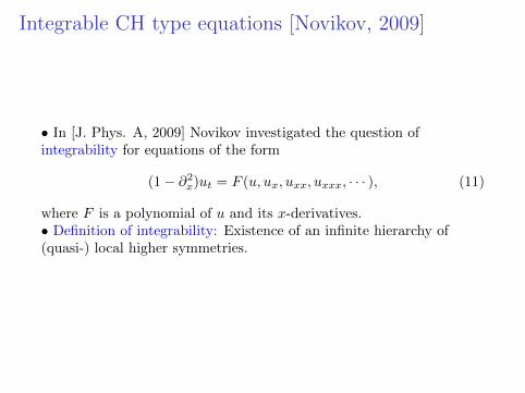
• In [J. Phys. A, 2009] Novikov investigated the question ofintegrability for equations of the form

(1− ∂2x)ut = F (u, ux, uxx, uxxx, · · · ), (11)

where F is a polynomial of u and its x-derivatives.• Definition of integrability: Existence of an infinite hierarchy of(quasi-) local higher symmetries.

Integrable CH type equations [Novikov, 2009] (cont.)

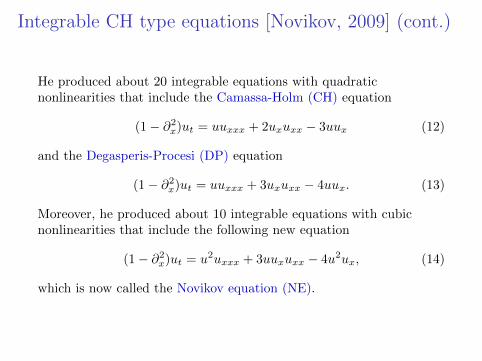
He produced about 20 integrable equations with quadraticnonlinearities that include the Camassa-Holm (CH) equation

(1− ∂2x)ut = uuxxx + 2uxuxx − 3uux (12)

and the Degasperis-Procesi (DP) equation

(1− ∂2x)ut = uuxxx + 3uxuxx − 4uux. (13)

Moreover, he produced about 10 integrable equations with cubicnonlinearities that include the following new equation

(1− ∂2x)ut = u2uxxx + 3uuxuxx − 4u2ux, (14)

which is now called the Novikov equation (NE).

Camassa and Holm approach

Camassa and Holm derived CH from the Euler equations ofhydrodynamics using asymptotic expansions. Also, they derived itspeakon solutions.

Concerning the hydrodynamical relevance of the Camassa-Holmequation as well as alternative derivations, we refers the reader to theworks by Johnson [2002, 2003], Constantin and Lannes [2009], andIonescu-Kruse [2007] and the references therein.

Fokas-Fuchssteiner approach

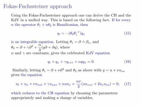
Using the Fokas-Fuchssteiner approach one can derive the CH and theKdV in a unified way. This is based on the following fact. If for everyn the operator θ1 + nθ2 is Hamiltonian, then

qt = −(θ2θ−11 )qx (15)

is an integrable equation. Letting θ1 = ∂.= ∂x, and

θ2 = ∂ + γ∂3 +α

3(q∂ + ∂q), where

α and γ are constants, gives the celebrated KdV equation

qt + qx + γqxxx + αqqx = 0. (16)

Similarly, letting θ1 = ∂ + ν∂3 and θ2 as above with q = u+ νuxxgives the equation

ut + ux + νuxxt + γuxxx + αuux +αν

3(uuxxx + 2uxuxx) = 0, (17)

which reduces to the CH equation by choosing the parametersappropriately and making a change of variables.

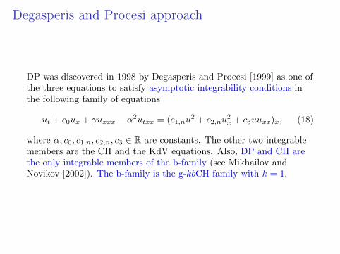
Degasperis and Procesi approach

DP was discovered in 1998 by Degasperis and Procesi [1999] as one ofthe three equations to satisfy asymptotic integrability conditions inthe following family of equations

ut + c0ux + γuxxx − α2utxx = (c1,nu2 + c2,nu

2x + c3uuxx)x, (18)

where α, c0, c1,n, c2,n, c3 ∈ R are constants. The other two integrablemembers are the CH and the KdV equations. Also, DP and CH arethe only integrable members of the b-family (see Mikhailov andNovikov [2002]). The b-family is the g-kbCH family with k = 1.

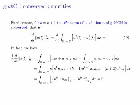
g-kbCH conserved quantities

Furthermore, for b = k + 1 the H1-norm of a solution u of g-kbCH isconserved, that is

d

dt‖u(t)‖2H1 =

d

dt

∫R or T

[u2(t) + u2x(t)

]dx = 0. (19)

In fact, we have

1

2

d

dt‖u(t)‖2H1 =

∫R or T

[uut + uxuxt

]dx =

∫R or T

u[ut − uxxt

]dx

=

∫R or T

u[ukuxxx + (k + 1)uk−1uxuxx − (k + 2)ukux

]dx

=

∫R or T

[ (uk+1uxx

)x−(uk+2

)x

]dx = 0.

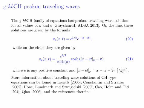
g-kbCH peakon traveling waves

The g-kbCH family of equations has peakon traveling wave solutionfor all values of k and b [Grayshan-H, ADSA 2013]. On the line, thesesolutions are given by the formula

uc(x, t) = c1/ke−|x−ct|, (20)

while on the circle they are given by

uc(x, t) =c1/k

cosh(π)cosh ([x− ct]p − π) , (21)

where c is any positive constant and [x− ct]p.= x− ct− 2π

[x−ct2π

].

More information about traveling wave solutions of CH typeequations can be found in Lenells [2005], Constantin and Strauss[2002], Hone, Lundmark and Szmigielski [2009], Cao, Holm and Titi[204], Qiao [2006], and the references therein.

u(x, t) =c

2sech2

(√c

2(x− ct)

), u(x, t) = c1/ke−|x−ct|

Figure: KdV soliton & g-kbCH peakon

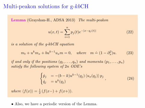
Multi-peakon solutions for g-kbCH

Lemma (Grayshan-H., ADSA 2013) The multi-peakon

u(x, t) =

n∑i=1

pj(t)e−|x−qj(t)| (22)

is a solution of the g-kbCH equation

mt + ukmx + buk−1uxm = 0, where m.= (1− ∂2x)u. (23)

if and only if the positions (q1, . . . , qn) and momenta (p1, . . . , pn)satisfy the following system of 2n ODE’s

pj = −(b− k)uk−1(qj) 〈ux(qj)〉 pjqj = uk(qj)

, (24)

where 〈f(x)〉 = 12 (f(x−) + f(x+)).

• Also, we have a periodic version of the Lemma.

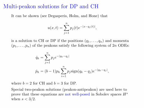
Multi-peakon solutions for DP and CH

It can be shown (see Degasperis, Holm, and Hone) that

u(x, t) =

n∑j=1

pj(t)e−|x−qj(t)|,

is a solution to CH or DP if the positions (q1, . . . , qn) and momenta(p1, . . . , pn) of the peakons satisfy the following system of 2n ODEs:

qk =

n∑j=1

pje−|qk−qj |

pk = (b− 1)pk

n∑i=1

pjsign(qk − qj)e−|qk−qj |,

where b = 2 for CH and b = 3 for DP.

Special two-peakon solutions (peakon-antipeakon) are used here toprove that these equations are not well-posed in Sobolev spaces Hs

when s < 3/2.

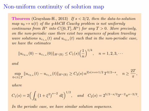
Non-uniform continuity of solution map

Theorem (Grayshan-H., 2013) If s < 3/2, then the data-to-solutionmap u0 7→ u(t) of the g-kbCH Cauchy problem is not uniformlycontinuous from Hs into C([0, T ], Hs) for any T > 0. More precisely,on the non-periodic case there exist two sequences of peakon travelingwave solutions uc1,n(t) and uc2,n(t) such that in the non-periodic case,we have the estimates

‖uc2,n(0)− uc1,n(0)‖Hs(R) ≤ C1(s)( 1

n

)1/k, n = 1, 2, 3, · · ·

and

sup0<t≤T

‖uc2,n(t)− uc1,n(t)‖Hs(R) ≥ C2(s)n2|s|+s+1/2 T 3/2−s, n ≥ 2T

π,

where

C1(s) = 2(∫

R

(1 + ξ2

)s−2dξ)1/2

, and C2(s) = 25/2−s/23s−2πs−3/2.

In the periodic case, we have similar solution sequences.

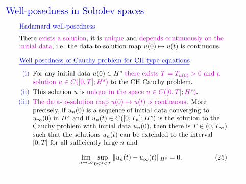
Well-posedness in Sobolev spaces

Hadamard well-posedness

There exists a solution, it is unique and depends continuously on theinitial data, i.e. the data-to-solution map u(0) 7→ u(t) is continuous.

Well-posedness of Cauchy problem for CH type equations

(i) For any initial data u(0) ∈ Hs there exists T = Tu(0) > 0 and asolution u ∈ C([0, T ];Hs) to the CH Cauchy problem.

(ii) This solution u is unique in the space u ∈ C([0, T ];Hs).

(iii) The data-to-solution map u(0) 7→ u(t) is continuous. Moreprecisely, if un(0) is a sequence of initial data converging tou∞(0) in Hs and if un(t) ∈ C([0, Tn];Hs) is the solution to theCauchy problem with initial data un(0), then there is T ∈ (0, T∞)such that the solutions un(t) can be extended to the interval[0, T ] for all sufficiently large n and

limn→∞

sup0≤t≤T

‖un(t)− u∞(t)‖Hs = 0. (25)

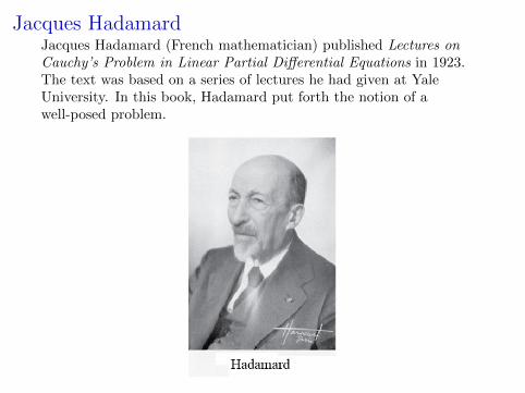
Jacques HadamardJacques Hadamard (French mathematician) published Lectures onCauchy’s Problem in Linear Partial Differential Equations in 1923.The text was based on a series of lectures he had given at YaleUniversity. In this book, Hadamard put forth the notion of awell-posed problem.

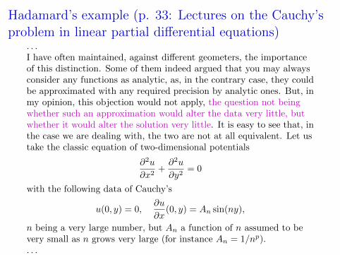
Hadamard’s example (p. 33: Lectures on the Cauchy’sproblem in linear partial differential equations)

. . .I have often maintained, against different geometers, the importanceof this distinction. Some of them indeed argued that you may alwaysconsider any functions as analytic, as, in the contrary case, they couldbe approximated with any required precision by analytic ones. But, inmy opinion, this objection would not apply, the question not beingwhether such an approximation would alter the data very little, butwhether it would alter the solution very little. It is easy to see that, inthe case we are dealing with, the two are not at all equivalent. Let ustake the classic equation of two-dimensional potentials

∂2u

∂x2+∂2u

∂y2= 0

with the following data of Cauchy’s

u(0, y) = 0,∂u

∂x(0, y) = An sin(ny),

n being a very large number, but An a function of n assumed to bevery small as n grows very large (for instance An = 1/np).. . .

These data differ from zero as little as can be wished. Nevertheless,such a Cauchy problem has for its solution

u =Ann

sin(ny)Sh(nx),

which, if An = 1n , 1

np , e−√n, is very large for any determinate value of

x different from zero on account of the mode of growth of enx andconsequently Sh(nx).In this case, the presence of the factor sin ny produces a “fluting” ofthe surface, and we see that this fluting, however imperceptible in theimmediate neighbourhood of the y-axis, becomes enormous at anygiven distance of it however small, provided the fluting be takensufficiently thin by taking n sufficiently great.

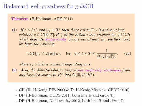
Hadamard well-posedness for g-kbCH

Theorem (H-Holliman, ADE 2014)

(1) If s > 3/2 and u0 ∈ Hs then there exists T > 0 and a uniquesolution u ∈ C([0, T ];Hs) of the initial value problem for g-kbCHwhich depends continuously on the initial data u0. Furthermore,we have the estimate

‖u(t)‖Hs ≤ 2‖u0‖Hs , for 0 ≤ t ≤ T ≤ 1

2kcs‖u0‖kHs, (26)

where cs > 0 is a constant depending on s.

(2) Also, the data-to-solution map is not uniformly continuous fromany bounded subset in Hs into C([0, T ];Hs).

- CH (R: H-Kenig DIE 2009 & T: H-Kenig-Misiolek, CPDE 2010)

- DP (H-Holliman, DCDS 2011, both line R and circle T)

- DP (H-Holliman, Nonlinearity 2012, both line R and circle T)

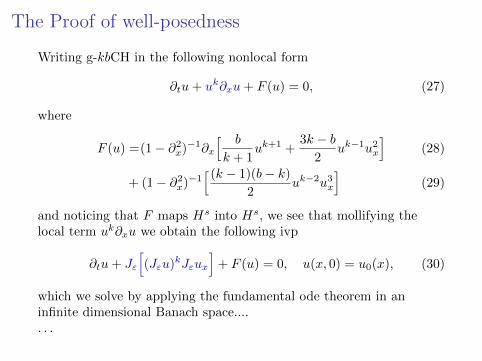
The Proof of well-posedness

Writing g-kbCH in the following nonlocal form

∂tu+ uk∂xu+ F (u) = 0, (27)

where

F (u) =(1− ∂2x)−1∂x

[ b

k + 1uk+1 +

3k − b2

uk−1u2x

](28)

+ (1− ∂2x)−1[ (k − 1)(b− k)

2uk−2u3x

](29)

and noticing that F maps Hs into Hs, we see that mollifying thelocal term uk∂xu we obtain the following ivp

∂tu+ Jε

[(Jεu)kJεux

]+ F (u) = 0, u(x, 0) = u0(x), (30)

which we solve by applying the fundamental ode theorem in aninfinite dimensional Banach space..... . .

The Proof of non-uniform continuity (more to come!)Choosing the approximate solutions

uω,n(x, t).= ωn−1/k + n−s cos(nx− ωt), (31)

where ω = −1, 1 if k is odd and ω = 0, 1 if k is even, we see that theysatisfy the three conditions of nonuniform continuity, that is:

• They are bounded.

• At t = 0 the Hs distance of their difference goes to zero.

• And, at any later time t > 0 this distance it is bounded below by apositive constant depending on t.

Then, solving the Cauchy problem with initial data the value of theapproximate solutions at t = 0 we obtain two sequences of actualsolutions with common lifespan and whose difference from theapproximate solutions is negligible. This allow us to show that thesequences of these solutions satisfy the conditions of nonuniformdependence.We begin by substituting the approximate solutions (31) into g-kbCH,giving rise to “small” error E, i.e.

‖E .= ∂tu

ω,n + (uω,n)k∂xuω,n + F (uω,n)‖Hσ . n−rs . (32)

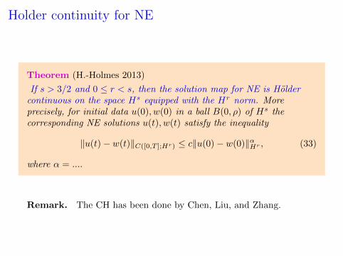
Holder continuity for NE

Theorem (H.-Holmes 2013)

If s > 3/2 and 0 ≤ r < s, then the solution map for NE is Holdercontinuous on the space Hs equipped with the Hr norm. Moreprecisely, for initial data u(0), w(0) in a ball B(0, ρ) of Hs thecorresponding NE solutions u(t), w(t) satisfy the inequality

‖u(t)− w(t)‖C([0,T ];Hr) ≤ c‖u(0)− w(0)‖αHr , (33)

where α = ....

Remark. The CH has been done by Chen, Liu, and Zhang.

I``-posedness for CH and DP

Theorem (DP by H-Holliman-Grayshan, CPDE 2014. CH by Byers)

For s < 3/2 the Cauchy problem for CH and DP on both the line andthe circle, is not well-posed in Hs in the sense of Hadamard.

The Proof is based on:

• Conserved quantities (H1 for CH and twisted L2 for DP).

• The interaction of peakon-antipeakon traveling wave solutions.

Open Problem: Is CH and DP well-posed at the critical Sobolevexponent s = 3/2?

The FORQ equation – Not a member of g-kbCH!

The FORQ equation

(1− ∂2x)ut = ∂x(−u3 + uu2x + u2uxx − u2xuxx) (34)

was derived independently by

• Fokas (Phys. D 1995), as an integrable generalisation of themodified KdV equation via a bi-Hamiltonian systems approach.

• Olver & Rosenau (Phys. Rev. E 1996), via a similar method butin a different form. This equation was also derived byFuchssteiner.

• Qiao (J. Math. Phys. 2006), as an approximation to Eulerequations. Qiao also showed that FORQ admits cusped andW/M soliton travelling waves.

It can be written in the following nonlocal form

∂tu = −u2∂xu+1

3(∂xu)3 −

(1− ∂2x

)−1 [1

3(∂xu)

3

]− ∂x

(1− ∂2x

)−1 [2

3u3 + u (∂xu)

2

].

FORQ Cauchy problem

Theorem (H-Mantzavinos, Nonlinear Anal. 2014)

(1) If s > 5/2 and u0 ∈ Hs, then there exists T > 0 and a uniquesolution u ∈ C

([0, T ];Hs

)of the FORQ ivp, formulated either on

the line or on the circle, which depends continuously on theinitial data u0. Moreover, we have the estimate

‖u(t)‖Hs ≤ 2‖u0‖Hs for 0 ≤ t ≤ T ≤ 1

4cs‖u0‖2Hs

where cs > 0 is a constant depending on s.

(2) Also, the data-to-solution map is not uniformly continuous fromany bounded subset in Hs into C([0, T ];Hs).

Peakon travelling wavesFor the purpose of finding travelling wave solutions of the formu(x, t) = f(x− ct), we consider the FORQ in the local form

(1− ∂2x)ut +(1− 1

3∂2x

)∂x(u3) + 1

3∂2x(u3x) + ∂x(uu2x) = 0.

Lemma

1. (H-Mantzavinos, 2013) The 2π−periodic peakon

u(x, t) = γ√c cosh

([x− c t]p − π

), [x−c t]p = x−c t−2π

⌊x− c t

2π

⌋,

is a weak solution of FORQ iff γ = ±(1 +

2

3sinh2 π

)− 12 .

2. (Gui, Liu, Olver & Qu: CMP 2012) The non-periodic peakon

u(x, t) = α√c e−|x−c t|

is a weak solution iff α = ±√

3

2.

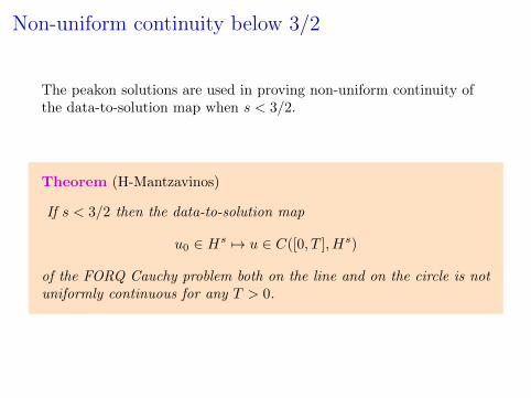
Non-uniform continuity below 3/2

The peakon solutions are used in proving non-uniform continuity ofthe data-to-solution map when s < 3/2.

Theorem (H-Mantzavinos)

If s < 3/2 then the data-to-solution map

u0 ∈ Hs 7→ u ∈ C([0, T ], Hs)

of the FORQ Cauchy problem both on the line and on the circle is notuniformly continuous for any T > 0.

Holder continuity for FORQ

Theorem (H-Mantzavinos, JNLS 2014)

If s > 5/2 and 0 ≤ r < s, then the solution map for FORQ is Holdercontinuous on the space Hs equipped with the Hr norm. Moreprecisely, . . .

Nonuniform continuity for CH

The Proof of non-uniform continuity for CH on T

We shall prove that there exist two sequences of CH solutions un(t)and vn(t) in C([0, T ];Hs(T)) such that:

• supn‖un(t)‖Hs + sup

n‖vn(t)‖Hs . 1,

• limn→∞

‖un(0)− vn(0)‖Hs = 0

• lim infn‖un(t)− vn(t)‖Hs & sin t, 0 ≤ t < T ≤ 1.

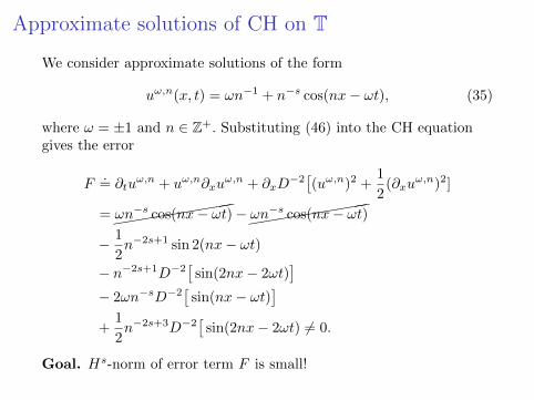
Approximate solutions of CH on T

We consider approximate solutions of the form

uω,n(x, t) = ωn−1 + n−s cos(nx− ωt), (35)

where ω = ±1 and n ∈ Z+. Substituting (46) into the CH equationgives the error

F.= ∂tu

ω,n + uω,n∂xuω,n + ∂xD

−2[(uω,n)2 +1

2(∂xu

ω,n)2]

=(((((((((ωn−s cos(nx− ωt)−(((((((((

ωn−s cos(nx− ωt)

− 1

2n−2s+1 sin 2(nx− ωt)

− n−2s+1D−2[

sin(2nx− 2ωt)]

− 2ωn−sD−2[

sin(nx− ωt)]

+1

2n−2s+3D−2

[sin(2nx− 2ωt) 6= 0.

Goal. Hs-norm of error term F is small!

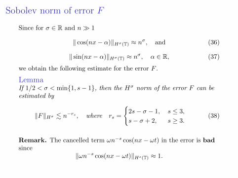
Sobolev norm of error F

Since for σ ∈ R and n 1

‖ cos(nx− α)‖Hσ(T) ≈ nσ, and (36)

‖ sin(nx− α)‖Hσ(T) ≈ nσ, α ∈ R, (37)

we obtain the following estimate for the error F .

LemmaIf 1/2 < σ < min1, s− 1, then the Hσ norm of the error F can beestimated by

‖F‖Hσ . n−rs , where rs =

2s− σ − 1, s ≤ 3,

s− σ + 2, s ≥ 3.(38)

Remark. The cancelled term ωn−s cos(nx− ωt) in the error is badsince

‖ωn−s cos(nx− ωt)‖Hs(T) ≈ 1.

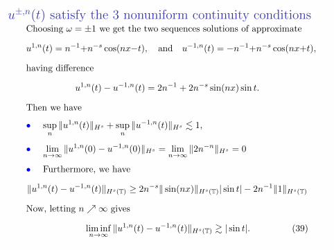
u±,n(t) satisfy the 3 nonuniform continuity conditionsChoosing ω = ±1 we get the two sequences solutions of approximate

u1,n(t) = n−1+n−s cos(nx−t), and u−1,n(t) = −n−1+n−s cos(nx+t),

having difference

u1,n(t)− u−1,n(t) = 2n−1 + 2n−s sin(nx) sin t.

Then we have

• supn‖u1,n(t)‖Hs + sup

n‖u−1,n(t)‖Hs . 1,

• limn→∞

‖u1,n(0)− u−1,n(0)‖Hs = limn→∞

‖2n−n‖Hs = 0

• Furthermore, we have

‖u1,n(t)− u−1,n(t)‖Hs(T) ≥ 2n−s‖ sin(nx)‖Hs(T)| sin t| − 2n−1‖1‖Hs(T)

Now, letting n∞ gives

lim infn→∞

‖u1,n(t)− u−1,n(t)‖Hs(T) & | sin t|. (39)

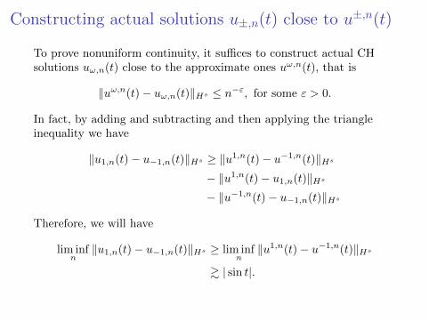
Constructing actual solutions u±,n(t) close to u±,n(t)

To prove nonuniform continuity, it suffices to construct actual CHsolutions uω,n(t) close to the approximate ones uω,n(t), that is

‖uω,n(t)− uω,n(t)‖Hs ≤ n−ε, for some ε > 0.

In fact, by adding and subtracting and then applying the triangleinequality we have

‖u1,n(t)− u−1,n(t)‖Hs ≥ ‖u1,n(t)− u−1,n(t)‖Hs− ‖u1,n(t)− u1,n(t)‖Hs− ‖u−1,n(t)− u−1,n(t)‖Hs

Therefore, we will have

lim infn‖u1,n(t)− u−1,n(t)‖Hs ≥ lim inf

n‖u1,n(t)− u−1,n(t)‖Hs

& | sin t|.

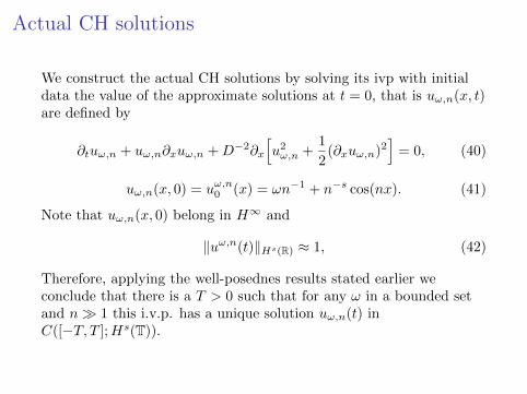
Actual CH solutions

We construct the actual CH solutions by solving its ivp with initialdata the value of the approximate solutions at t = 0, that is uω,n(x, t)are defined by

∂tuω,n + uω,n∂xuω,n +D−2∂x

[u2ω,n +

1

2(∂xuω,n)2

]= 0, (40)

uω,n(x, 0) = uω,n0 (x) = ωn−1 + n−s cos(nx). (41)

Note that uω,n(x, 0) belong in H∞ and

‖uω,n(t)‖Hs(R) ≈ 1, (42)

Therefore, applying the well-posednes results stated earlier weconclude that there is a T > 0 such that for any ω in a bounded setand n 1 this i.v.p. has a unique solution uω,n(t) inC([−T, T ];Hs(T)).

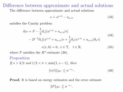
Difference between approximate and actual solutionsThe difference between approximate and actual solutions

v.= uω,n − uω,n (43)

satisfies the Cauchy problem

∂tv = F − 1

2∂x[(uω,n + uω,n)v]

−D−2∂x[(uω,n + uω,n)v +1

2∂x(uω,n + uω,n)∂xv]

(44)

v(x, 0) = 0, x ∈ T, t ∈ R, (45)

where F satisfies the Hσ-estimate (38).

PropositionIf s > 3/2 and 1/2 < σ < min1, s− 1, then

‖v(t)‖Hσ . n−rs . (46)

Proof. It is based on energy estimates and the error estimate

‖F‖Hσ . n−rs .

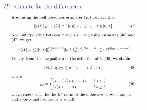
Hs estimate for the difference v

Also, using the well-posedness estimates (26) we have that

‖v(t)‖Hs+1 . ‖uω,n(0)‖Hs+1 . n, t ∈ [0, T ]. (47)

Now, interpolating between σ and s+ 1 and using estimates (46) and(47) we get

‖v(t)‖Hs ≤ ‖v(t)‖1/(s+1−σ)Hσ ‖v(t)‖(s−σ)/(s+1−σ)

Hs+1 . n−1

s+1−σ (rs−s+σ).

Finally, from this inequality and the definition of rs (49) we obtain

‖v(t)‖Hs(T) . n−ρs , t ∈ [0, T ], (48)

where

ρs =

(s− 1)/(s+ 1− σ), if s ≤ 3

2/(s+ 1− σ), if s ≥ 3,(49)

which shows that the the Hs norm of the difference between actualand approximate solutions is small!

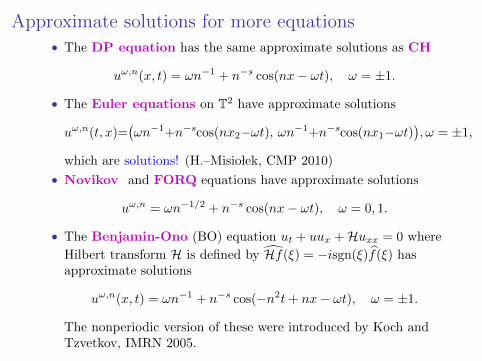
Approximate solutions for more equations• The DP equation has the same approximate solutions as CH

uω,n(x, t) = ωn−1 + n−s cos(nx− ωt), ω = ±1.

• The Euler equations on T2 have approximate solutions

uω,n(t, x)=(ωn−1+n−scos(nx2−ωt), ωn−1+n−scos(nx1−ωt)

), ω = ±1,

which are solutions! (H.–Misio lek, CMP 2010)

• Novikov and FORQ equations have approximate solutions

uω,n = ωn−1/2 + n−s cos(nx− ωt), ω = 0, 1.

• The Benjamin-Ono (BO) equation ut + uux +Huxx = 0 where

Hilbert transform H is defined by Hf(ξ) = −isgn(ξ)f(ξ) hasapproximate solutions

uω,n(x, t) = ωn−1 + n−s cos(−n2t+ nx− ωt), ω = ±1.

The nonperiodic version of these were introduced by Koch andTzvetkov, IMRN 2005.

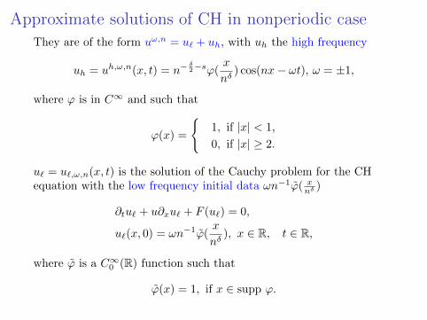
Approximate solutions of CH in nonperiodic case

They are of the form uω,n = u` + uh, with uh the high frequency

uh = uh,ω,n(x, t) = n−δ2−sϕ(

x

nδ) cos(nx− ωt), ω = ±1,

where ϕ is in C∞ and such that

ϕ(x) =

1, if |x| < 1,

0, if |x| ≥ 2.

u` = u`,ω,n(x, t) is the solution of the Cauchy problem for the CHequation with the low frequency initial data ωn−1ϕ( x

nδ)

∂tu` + u∂xu` + F (u`) = 0,

u`(x, 0) = ωn−1ϕ(x

nδ), x ∈ R, t ∈ R,

where ϕ is a C∞0 (R) function such that

ϕ(x) = 1, if x ∈ supp ϕ.

Analytic theory

Cauchy Problem for CH equations

Multiplying by the inverse of (1− ∂2x), we write the Cauchy problemfor CH, DP, NE and FORQ equations in the following unified way

ut = (1− ∂2x)−1P (u).= F (u), u(0) = u0. (50)

where, P (u) is given by the right hand-sides of equations (12), (13),(14) and (34).

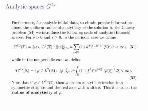
Analytic spaces Gδ,s

Furthermore, for analytic initial data, to obtain precise informationabout the uniform radius of analyticity of the solution to the Cauchyproblem (54) we introduce the following scale of analytic (Banach)spaces. For δ > 0 and s ≥ 0, in the periodic case we define

Gδ,s(T) = ϕ ∈ L2(T) : ||ϕ||2Gδ,s=∑k∈Z

(1+k2)se2δ|k||ϕ(k)|2 <∞, (51)

while in the nonperiodic case we define

Gδ,s(R) = ϕ ∈ L2(R) : ||ϕ||2Gδ,s=∫R

(1 + ξ2)se2δ|ξ||ϕ(ξ)|2dξ <∞.

(52)Note that if ϕ ∈ Gδ,s(T) then ϕ has an analytic extension to asymmetric strip around the real axis with width δ. This δ is called theradius of analyticity of ϕ.

Well-posedness of CH equations in analytic spaces

Theorem (Barostichi-H.-Petronilho, JFA 2015)Let s > 1

2 . If u0 ∈ G1,s+2 on the circle or the line, then there exists apositive time T , which depends on the initial data u0 and s, such thatfor every δ ∈ (0, 1), the Cauchy problem (54) has a unique solution uwhich is a holomorphic function in the disc D(0, T (1− δ)) valued inGδ,s+2. Furthermore, the analytic lifespan T satisfies the estimate

T ≈ 1

||u0||kG1,s

, (53)

where k = 1 for the CH and DP equations and k = 2 for the NE andFORQ equations.

Theorem (Barostichi-H.-Petronilho, JFA 2015)If s > 1

2 , then the data-to-solution map u(0) 7→ u(t) of the Cauchyproblem (54) for the CH equations is continuous from Gδ,s+2 into thesolutions space.

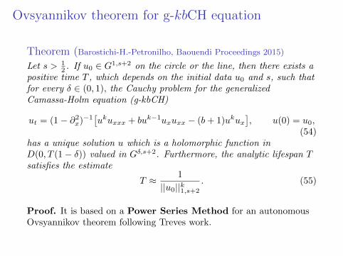
Ovsyannikov theorem for g-kbCH equation

Theorem (Barostichi-H.-Petronilho, Baouendi Proceedings 2015)

Let s > 12 . If u0 ∈ G1,s+2 on the circle or the line, then there exists a

positive time T , which depends on the initial data u0 and s, such thatfor every δ ∈ (0, 1), the Cauchy problem for the generalizedCamassa-Holm equation (g-kbCH)

ut = (1− ∂2x)−1[ukuxxx + buk−1uxuxx − (b+ 1)ukux

], u(0) = u0,

(54)has a unique solution u which is a holomorphic function inD(0, T (1− δ)) valued in Gδ,s+2. Furthermore, the analytic lifespan Tsatisfies the estimate

T ≈ 1

||u0||k1,s+2

. (55)

Proof. It is based on a Power Series Method for an autonomousOvsyannikov theorem following Treves work.

Thanks!