The Caughey absorbing layer method – implementation … · This paper addresses the Caughey Absorbing Layer Method ... validation in Ansys software . ... a parametric optimization

1540

Abstract This paper addresses the Caughey Absorbing Layer Method (CALM) performance in the one-dimensional problem and its implementation in commercial software, with possibility of direct extension to two-dimensions. The adequacy and numerical efficiency is evaluated using three different error measures and five different variations of the damping profile. Other parameters that are subjected to evaluation are the length of the absorbing layer in relation to the wavelength to absorb, the value of the loss factor at the end of the absorbing layer, and the ratio of the load to layer frequency. The problem is firstly analysed theoretically, resulting in estimates for the wave reflection due to transition and truncation of the model. In order to confirm that no spurious waves will be present in the finite element solution, the numerical implementation is validated by com-parison with the analytical solution. The analysis of the error measures on the numerical results obtained for various combinations of the model’s parameters lead to the conclu-sion that CALM is effective at mitigating waves reflected from the boundaries. The optimum loss factor as a function of the ratio of the length of the absorbing layer to the wavelength to absorb is deter-mined through parametric analyses. Although the optimal damping is frequency dependent, it was shown that the CALM’s effectiveness can be extended to a wider range of frequencies by increasing the smooth-ness of the damping profile. Keywords Elastic wave propagation; finite element method; absorbing boundary layer; unbounded domains.

The Caughey absorbing layer method – implementation and validation in Ansys software

1 INTRODUCTION

One of the most significant difficulties in the numerical study of elastic wave propagation in solids, particularly when using the finite element (FE) method (see Hughes (1987)), is the difficulty to simulate semi-infinite or unbounded domains.

André Rodriguesa

Zuzana Dimitrovováb

aUNIC, Departamento de Engenharia Civil, Faculdade de Ciências e Tecnologia, Universidade Nova de Lisboa, Portugal bDepartamento de Engenharia Civil, Faculdade de Ciências e Tecnologia, Universidade Nova de Lisboa, Portugal bIDMEC, Instituto Superior Técnico, Universidade de Lisboa, Portugal Corresponding author: [email protected] [email protected] http://dx.doi.org/10.1590/1679-78251713 Received 21.11.2014 In revised form 13.04.2015 Accepted 22.04.2015 Available online 02.05.2015

1541 A. Rodrigues and Z. Dimitrovová / The Caughey absorbing layer method – implementation and validation in Ansys software

For example, in the analysis of soil vibrations, the soil region is neither confined to a closed space nor isolated from the surroundings. This means that modelling the area of interest without special considerations will result in reflections of the elastic waves at the boundaries of the model. These reflections will become superimposed with the actual solution, making it inaccurate. As the waves are locked inside the finite domain, the energy is not released as it happens in reality. In an analytical analysis, it is common to admit the soil as a semi-infinite medium. This ap-proach was employed by Boussinesq, who studied the stresses on the soil due to a static load (see Karol (1960)). Since the domain of most numerical methods must be itself finite, various truncation techniques have been proposed over the last decades, such as: (i) local absorbing boundary condi-tions (Lysmer and Kuhlemeyer, 1969; Lindman, 1975; Engquist and Majda, 1977, 1979); (ii) the boundary element method (Banerjee and Butterfield, 1981); (iii) the infinite element method (Bet-tess, 1977); (iv) absorbing layers, including Perfectly Matched Layers (PML, Bérenger (1994)) and the Caughey Absorbing Layer Method (CALM, Semblat et al. (2011)). The local absorbing boundary conditions are among the simpler methods. They are implemented as dampers at the boundary, whose properties are derived from changing the wave equation to ad-mit only outgoing waves. The Lysmer-Kuhlemeyer boundary in particular uses damping coefficients that are proportional to the mass density of the medium and the speed of the waves to absorb. The rate of absorption depends on the angle of incidence of the wave, and is usually tuned to perfectly absorb only at normal incidence. Although effective for simple problems, absorbing boundaries may lead to instabilities at discontinuities (such as layers with different mechanical properties). Fur-thermore, in order to avoid rigid body motion, these boundary conditions must be complemented with additional elements, like springs, whose stiffness is difficult to estimate. The boundary element method changes the nature of the numerical problem, from a volume discretisation to a boundary discretisation. This requires a fundamental solution that satisfies the appropriate conditions at infinity. For dynamical problems, the Sommerfeld’s radiation condition is used, which states that “the energy … radiated from the sources must scatter to infinity; no energy may be radiated from infinity into ... the field” (Sommerfeld, 1949). Although the BEM is very ro-bust, the computational cost is much higher than traditional FE – for many problems where the surface to volume ratio is high, the boundary method may be less efficient than volume-discretisation methods (see Katsikadelis (2002)). The infinite element method is closer to the traditional FE approach. It consists in modelling the interior domain with conventional finite elements and, at the model’s boundaries, introducing ele-ments with special shape functions. These special shape functions grow without bound as the coor-dinate approaches infinity, therefore simulating an infinite element. Unfortunately, only some com-mercial FE programs include this formulation. Absorbing layer methods have been widely used since the introduction of the PML by Bérenger (1994), based on previous absorbing layer formulations (e.g. Holland and Williams (1983)). The absorbing layer method applies a layer of material with some damping capability at the boundaries of the medium of interest. Waves behave normally inside the original medium, but decay as they travel inside the absorbing layer, attenuating or preventing reflections at the boundaries of the model. However, some reflection is expected to occur at the interface between the normal medium and the absorbing layers, due to the material discontinuity.

Latin American Journal of Solids and Structures 12 (2015) 1540-1564

A. Rodrigues and Z. Dimitrovová / The Caughey absorbing layer method – implementation and validation in Ansys software 1542

The PML in particular can be implemented with a complex coordinate stretching (see Chew and Weedon (1994)). The analytical formulation does not introduce reflections at the interface between the two materials (hence perfectly matched), but this property is partially lost after discretisation. The main drawback of the PML is that its implementation is not straightforward, particularly in the time domain – it requires a split-field formulation or convolution operations. This makes it diffi-cult to use in FE commercial software. The CALM, proposed by Semblat et al. (2011), is not perfectly matched, but much simpler to implement than the PML. The absorbing layer has the mechanical properties of the medium of interest, but exhibits Caughey (or Rayleigh) damping tuned to ensure that the rate of absorption for the desired frequency is above an arbitrary value. It has the advantage of being intrinsically multi-directional, unlike local absorbing boundaries and the PML. Since it only requires manipula-tion of the FE damping matrix, it can be easily implemented in FE commercial software. The au-thors have found promising results in the implementation of the CALM in the commercial FE soft-ware Ansys (see Kohnke (1999)) using an implicit dynamics formulation for one- and two-dimensional plane-stress problems (presented in Rodrigues and Dimitrovová (2014)). In the present paper, the authors implement the Rayleigh formulation of the CALM in the commercial FE software Ansys, using implicit time integration, for a one-dimensional plane-strain problem. The model is subjected to a displacement in one of its extremities, which follows a wavelet function with a well-defined dominant frequency, and therefore the wavelength inside the medium is also well-defined. The CALM’s performance is analysed using three different error measures: the maximum amplitude of the reflected waves, the maximum L2-norm of the reflected waves, and the time integration of the L2-norm of the reflected waves. It is observed that the optimum properties for the absorbing layer require a compromise between reducing round-trip and transition reflections. In this context round-trip reflection refers to the waves reflected at the end of the absorbing layer and transition reflection represent the waves that reflect at the interface between the medium of interest and the absorbing layer. Round-trip reflection can be reduced simply by increasing the damping in the layer, but this increases transition reflection. To mitigate this problem, the damping is introduced smoothly along the layer. Different variations of the damping profile are tested (constant, linear, quadratic, cubic and exponential) and their efficiency is compared. It is concluded that a variable damping profile leads to less reflections than constant damping across the absorbing layer. The linear variation is the most efficient for short layers, while the quadratic is best for long layers. For each damping profile, a parametric optimization is performed to obtain the optimum loss factor at the end of the layer as a function of the dimensionless ratio of the length of the absorbing layer to the wavelength to absorb. From this process, empirical estimates for the optimum loss fac-tor are proposed and shown to fit the numerical results almost perfectly for most cases. These for-mulas can be used to tune the CALM for different problems, as long as the wavelength to absorb can be estimated. Lastly, a sensitivity analysis is performed to determine how a difference between the frequency of the load and the frequency that the CALM is tuned to absorb affects the results. Unlike Semblat et al. (2011) suggested, the efficiency of the CALM does not increase with this difference, due to a higher transition reflection coefficient. However, it is seen that the higher order damping profiles are



less sensitive to this discrepancy, and may be a better choice for problems were a wide range of frequencies is present, or were the predominant frequency is not known. In brief, the new contributions of this paper are: (i) previously unpublished analytical estimates for the effectiveness of the CALM, which support the empirical observation that a compromise be-tween round-trip and transition reflections must be found; (ii) implementation of the CALM in Ansys implicit dynamics module (in particular the variable Rayleigh damping); (iii) empirical esti-mates for the optimum loss factor as a function of the ratio of the layer’s length to the wavelength for various damping profiles, which can be used to tune the CALM for different problems; (iv) demonstration of how the CALM’s effectiveness can be extended over a wider range of frequencies by employing a smoother damping profile. The paper is organized in the following way: in section 2, the theoretical principle behind the CALM is presented, theoretical values for the reflection coefficients are proposed, and the solution by modal superposition is discussed. Section 3 details the implementation of the CALM in the FE commercial software Ansys, which is then validated by comparison with the solution by modal su-perposition; the error measures are presented and then used to perform a parametrical optimization of the CALM parameters; lastly, a sensitivity analysis is performed. Section 4 summarizes the re-sults and discusses future work. 2 THE CAUGHEY ABSORBING LAYER METHOD

The Caughey Absorbing Layer Method was proposed by Semblat et al. (2011) as a simple and reli-able alternative to the Perfectly Matched Layer (PML). Like other absorbing layer methods, the CALM consists in defining an absorbing layer at the boundaries of the elastic medium under consideration. This absorbing layer is modelled with the same elastic properties as the interior medium, but damping is added to attenuate all waves that leave the interior domain. Unlike the classical formulation of the PML, the CALM presents multi-directional attenuating properties. To ensure that the absorbing layer exhibits the desired behaviour, the damping properties must be carefully chosen to apply an adequate level of attenuation to the relevant frequency. 2.1 The Rayleigh damping formulation

One of the simplest ways to define damping in FE analysis is to consider the Rayleigh formulation (see Liu and Gorman (1995)), where the damping matrix (C) is assumed to be a linear combination of the stiffness (K) and mass (M) matrixes: C M K (1) and are known as the Rayleigh coefficients. This approach is convenient because FE methods already require the assembly of the mass and stiffness matrices. It is well known (see, for example, Clough and Penzien (1993)) that the loss factor ( , the ratio of energy dissipated to the energy stored in the system for every oscillation) is approximately dou-



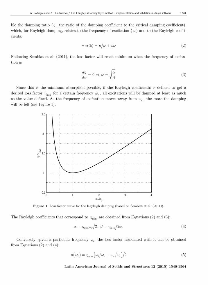
ble the damping ratio ( , the ratio of the damping coefficient to the critical damping coefficient), which, for Rayleigh damping, relates to the frequency of excitation ( ) and to the Rayleigh coeffi-cients: 2 (2) Following Semblat et al. (2011), the loss factor will reach minimum when the frequency of excita-tion is

0d

d

(3)

Since this is the minimum absorption possible, if the Rayleigh coefficients is defined to get a desired loss factor min for a certain frequency r , all excitations will be damped at least as much as the value defined. As the frequency of excitation moves away from r , the more the damping will be felt (see Figure 1).

Figure 1: Loss factor curve for the Rayleigh damping (based on Semblat et al. (2011)).

The Rayleigh coefficients that correspond to min are obtained from Equations (2) and (3): 2, 2min r min r (4)

Conversely, given a particular frequency i , the loss factor associated with it can be obtained from Equations (2) and (4): min 2i i r r i (5)



Semblat’s approach is to define the frequency of minimum attenuation, r , as being equal to the predominant frequency of the waves to absorb. In theory, this method ensures that all waves will be attenuated at least by a factor proportional to min . The Rayleigh damping coefficients to adopt are then calculated using Equation (4) for the predominant frequency and the desired minimum attenuation. However, this does not take into account that when the waves travel from the medium into the absorbing layer, the sudden introduction of damping causes reflections, the amplitude of which increases with the intensity of damping. This phenomenon will be discussed over the next sections. 2.2 Absorbing layer properties

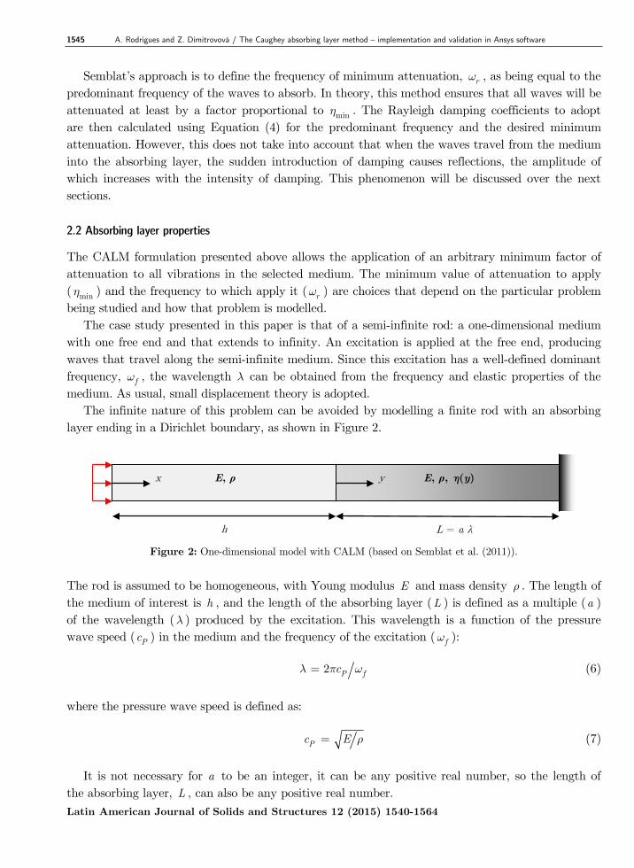
The CALM formulation presented above allows the application of an arbitrary minimum factor of attenuation to all vibrations in the selected medium. The minimum value of attenuation to apply ( min ) and the frequency to which apply it ( r ) are choices that depend on the particular problem being studied and how that problem is modelled. The case study presented in this paper is that of a semi-infinite rod: a one-dimensional medium with one free end and that extends to infinity. An excitation is applied at the free end, producing waves that travel along the semi-infinite medium. Since this excitation has a well-defined dominant frequency, f , the wavelength can be obtained from the frequency and elastic properties of the medium. As usual, small displacement theory is adopted. The infinite nature of this problem can be avoided by modelling a finite rod with an absorbing layer ending in a Dirichlet boundary, as shown in Figure 2.

Figure 2: One-dimensional model with CALM (based on Semblat et al. (2011)).

The rod is assumed to be homogeneous, with Young modulus E and mass density . The length of the medium of interest is h , and the length of the absorbing layer (L ) is defined as a multiple (a ) of the wavelength ( ) produced by the excitation. This wavelength is a function of the pressure wave speed ( Pc ) in the medium and the frequency of the excitation ( f ): 2 P fc (6) where the pressure wave speed is defined as: Pc E (7) It is not necessary for a to be an integer, it can be any positive real number, so the length of the absorbing layer, L , can also be any positive real number.

L = a λ h

y E, ρ, η(y) E, ρ x



The loss factor of the absorbing layer, y , is a function of the distance from the interface be-tween both media, y . This loss factor can either be constant ( y for 0,y L ) or increase monotonically along the layer, from no damping to maximum damping ( y : 0, 0,L ). The Rayleigh damping is then applied according to Equation (4). It has been noted (Oskooi, 2008; Oskooi et al., 2008; Oskooi and Johnson, 2011) that absorbing layers, like PMLs, perform better when a variable absorbing profile is defined. The smoothness of the variation was also found to influence their effectiveness. This is a result of the presence of two sources of reflection in the model: round-trip reflections and transition reflections. Round-trip reflection occurs because the absorbing layer never absorbs completely the incoming waves. As the waves travel along the layer, their amplitude decreases exponentially according to the loss factor, but they still reflect of the boundary condition and travel back into the medium of in-terest – hence the “round-trip” designation. Transition reflection occurs wherever there is a change of the properties of the medium of propa-gation. The steeper the variation, the higher the reflection will be. This is the case at the interface between the medium of interest and the absorbing layer when the loss factor is constant. This prob-lem is mitigated when the loss factor increases gradually along the layer. Although Semblat et al. (2011) tested the effectiveness of the CALM numerically and found that maximizing its effectiveness required finding a compromise between minimization of both types of reflections, no theoretical justification for this observation was provided. 2.2.1 Analytical solution by modal superposition

The problem of wave propagation in a single dimension due to an applied force at 0x can be expressed using the following differential equation: 2 , , ,Pc u x t u x t b x u x t P t x (8) where ,u x t is the displacement of the medium at the position x at time t , b x is the viscous damping, is the mass per length of the medium, P t is the magnitude of the force over time and x is the Dirac delta function. This problem can be solved by modal superposition, expressing the solution as the sum of an infinite number of functions:

1

, i ii

u x t v x q t

(9)

where iv x is known as the i -th undamped vibration mode and iq t is the corresponding gener-alized coordinate. For the boundary conditions shown in Figure 2 (free end at 0x , no displace-ment at x l h L ), the vibration modes are: cos , 2 1 2i i P i Pv x x c c i l (10) where i is the i -th undamped natural frequency. The generalized coordinates are the solutions to the system of equations



2

1 0

1 2d , 1,2,...,

l

i j i j ij

q t q t b x v x v x x q t P t il

(11)

If the damping is constant over the medium ( b x b ), then all equations are independent:

2

,2 2 , , 2 , 1,2,...,i i i i i i cr i cr iq t q t q t P t l b b b i (12)

In the case of the CALM, the damping ratio i for each frequency must be obtained from Equa-tion (5). Equation (12) allows one to obtain exact generalized coordinates for any desired mode. The sys-tem of equations (11), on the other hand, has to be solved numerically for a finite number of modes. In both cases an approximate solution is obtained by modal superposition. In the first case, if fur-ther precision is needed, one can solve Eq. (12) for higher modes and update the solution. In the second case, if higher modes are needed, the entire system of equations must be solved again. In the case of the CALM the damping is not constant over the length of the medium, and there-fore the system of equations (11) must be solved numerically. 2.2.2 Theoretical reflection coefficients

In the study of the phenomenon of reflection it is useful to introduce the concept of the reflection coefficient: the ratio between the amplitude of the reflected waves and the amplitude of the incom-ing waves (see Chapman (2004)). Although analytical expressions for the reflection coefficients asso-ciated with the PML have been published by Oskooi (2008), no such formulas exist yet for CALM. The round-trip reflection coefficient can be approximated by considering how much damping the waves are subjected to while traveling through the absorbing layer. By analogy with a single degree of freedom oscillator, it is assumed that the amplitude of the waves decays exponentially due to damping. This assumption was supported by the analytical solution of a rod with constant damping subjected to a sinusoidal force on the free-end (solving Equation (12) for sin fP t t ). The logarithmic decrement ( ) expresses the decrease in amplitude per cycle of oscillation, and is a function of the damping ratio , which is itself a function of the loss factor (Equation (2)): 2 22 1 1 4 (13) If the characteristics of the wave are known, it is possible to express the variation of the loga-rithmic decrement over the length of the absorbing layer as a function of y , since a cycle of oscillation occurs over the distance of a wavelength:

2d1 4

d d yy yy

(14)

where d y is the modified wavelength due to the presence of damping. This value can be ob-tained by considering the theoretical expression for the damped frequency:



221 1 4d d y y (15) which leads to the damped wavelength:

2 d

1 4dd

y

yyy

(16)

Since the waves must travel twice the length of the layer before returning to the medium of in-terest, the total decrease in amplitude after the round trip can be obtained by integrating (16) over

0,y L and multiplying by two. If one expresses the variable loss factor as the product of by a dimensionless damping profile s z : 0,1 0,1 , y s z z y L (17) the loss factor becomes:

1 1

0 02 d 2 d

Ls z z a s z z

(18)

Equation (18) shows that the loss factor is proportional to the area of the damping profile. A typical damping profile for absorbing layer techniques is a simple monomial equation of degree d ( ds z z , 0d ), for which the loss factor is: 2 1a d (19)

Since the amplitude of the waves decays exponentially, the round trip reflection coefficient is 2 1a d

RTR e (20)

It is evident from Equation (20) that increasing both the loss factor ( ) and the relative length of the layer (a ) reduces the amplitude of the reflected waves (by increasing the integral of the damping profile). Increasing the degree d of the damping profile increases the amplitude of the re-flected waves (it reduces the integral of the damping profile). However, increasing d leads to a smoother damping profile, which reduces the transition reflection (see Oskooi (2008)). Transition reflection can also be estimated theoretically. For a P-wave at normal incidence, it is well known (see Lowrie (2007)) that the transition reflection coefficient is: 1 ,1 2 ,2 1 ,1 2 ,2T P P P PR c c c c (21)

where 1 and 2 are the mass densities and ,1Pc and ,2Pc are the pressure wave velocities for the original medium and the new medium, respectively. This formula assumes a steep transition, and therefore can be only applied for y .



For the calculation of the damped wavelength, the wave velocity was assumed to be constant. However, for purposes of calculating the transition reflection, the wavelength can be assumed to be fixed and the wave velocity expressed as a function of the loss factor instead: 2 2 2

, 1 4 1 1 4 1 1 4P d P Tc c R (22)

For low damping, TR increases slowly with , but as gets closer to 2 (critical damping), TR grows very rapidly to 1 (total reflection of the incident waves). For 2 , oscillatory systems pre-sent super-critical damping, where no oscillation occurs. Therefore, Equation (21) is not valid for

2 , and the validity of Eq. (19) cannot be guaranteed as well. Unlike the round-trip reflection, the transition reflection coefficient for a damping profile with

0d is quite difficult to derive. Although some work has been done for linear variation (see Wolf (1937) and Liner and Bodmann (2010)), it is not directly applicable to the problem at hand. How-ever, Oskooi (2008) has shown numerically that TR decreases as both d and L increase. Particu-larly, for one-dimensional waves, Oskooi observed the following relation 2 21 , 0d

TR L d (23) According to Equations (20), (22) and (23), increasing reduces RTR but increases TR ; in-creasing a reduces RTR and TR if 0d (a longer layer results in a smoother transition); increasing d increases RTR but reduces TR . This is in accordance with the numerical results observed by Semblat et al. (2011): higher loss factor increases reflection at the interface, longer absorbing layers reduce round-trip reflection and a linear damping profile performs better than a constant one. 2.3 Limitations

In theory this methodology should work with any kind of dynamic analysis, both for time and fre-quency domain, since the use of Rayleigh damping ensures that the modes of vibration are uncou-pled. Preliminary tests have shown that the explicit central difference time integration method used by the LS-Dyna software (see Hallquist (2006)) requires an unreasonable computational cost to solve this problem – the time-step is five to six orders of magnitude lower than what is recommend-ed for the same problem without the desired damping. It is known that the stable time-step for explicit central difference time integration in the pres-ence of damping is: 2

max max max2 1t (24) where max is the frequency of the highest mode and max is the corresponding damping ratio. As the damping ratio increases, the stable time-step decreases. Since Rayleigh damping is felt more strongly in the higher modes, it is inevitable that it will lead to very small time-steps and therefore to high computation times. All models are therefore implemented in Ansys’ implicit dynamics mod-ule. Latin American Journal of Solids and Structures 12 (2015) 1540-1564


3 NUMERICAL IMPLEMENTATION

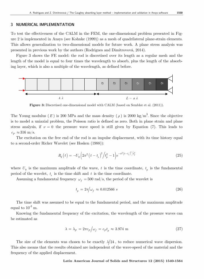
To test the effectiveness of the CALM in the FEM, the one-dimensional problem presented in Fig-ure 2 is implemented in Ansys (see Kohnke (1999)) as a mesh of quadrilateral plane-strain elements. This allows generalization to two-dimensional models for future work. A plane stress analysis was presented in previous work by the authors (Rodrigues and Dimitrovová, 2014). Figure 3 shows the FE model: the rod is discretised over its length as a regular mesh and the length of the model is equal to four times the wavelength to absorb, plus the length of the absorb-ing layer, which is also a multiple of the wavelength, as defined before.

Figure 3: Discretised one-dimensional model with CALM (based on Semblat et al. (2011)).

The Young modulus (E ) is 200 MPa and the mass density ( ) is 2000 kg/m3. Since the objective is to model a uniaxial problem, the Poisson ratio is defined as zero. Both in plane strain and plane stress analysis, if 0 the pressure wave speed is still given by Equation (7). This leads to

Pc 316 m/s. The excitation on the free end of the rod is an impulse displacement, with its time history equal to a second-order Ricker Wavelet (see Hosken (1988)):

22 222 22 0 2 1 s pt t t

s pR t U t t t e (25)

where 0U is the maximum amplitude of the wave, t is the time coordinate, pt is the fundamental period of the wavelet, st is the time shift and t is the time coordinate. Assuming a fundamental frequency f 500 rad/s, the period of the wavelet is 2 0.012566 p ft s (26)

The time shift was assumed to be equal to the fundamental period, and the maximum amplitude equal to 10-3 m. Knowing the fundamental frequency of the excitation, the wavelength of the pressure waves can be estimated as 2 3.974 mP P f P pc c t (27)

The size of the elements was chosen to be exactly 24 , to reduce numerical wave dispersion. This also means that the results obtained are independent of the wave-speed of the material and the frequency of the applied displacement.

4 λ L = a λ

η1 η2 η3 η4 η5 η6



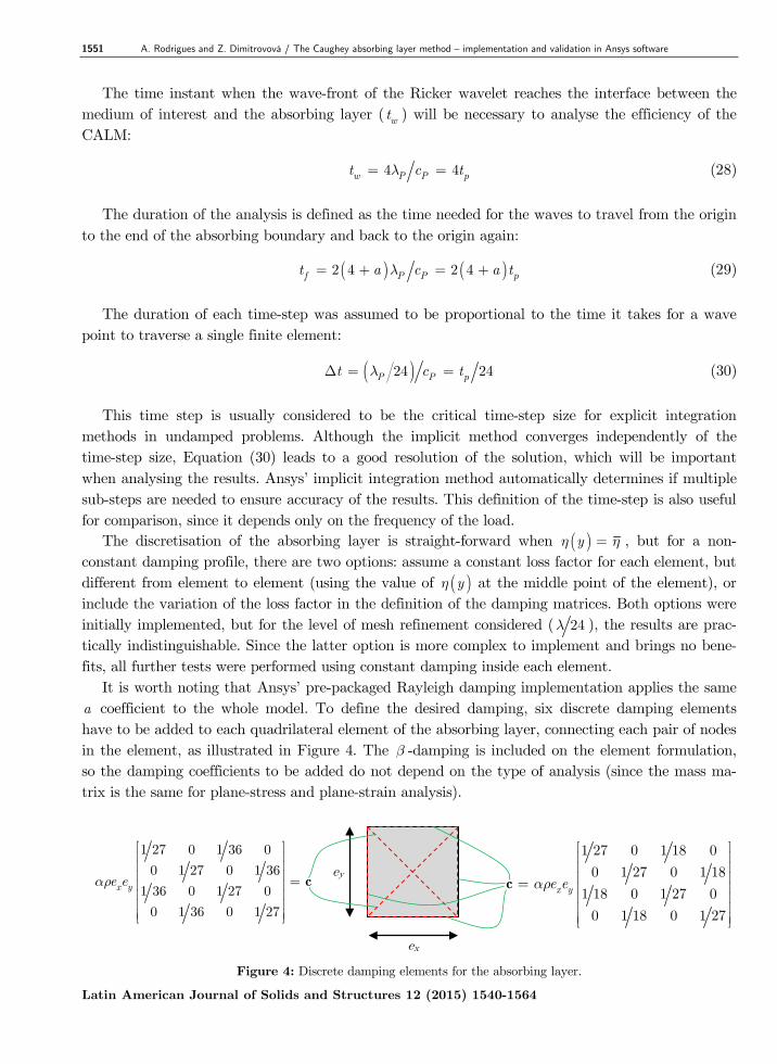
The time instant when the wave-front of the Ricker wavelet reaches the interface between the medium of interest and the absorbing layer ( wt ) will be necessary to analyse the efficiency of the CALM: 4 4w P P pt c t (28) The duration of the analysis is defined as the time needed for the waves to travel from the origin to the end of the absorbing boundary and back to the origin again: 2 4 2 4f P P pt a c a t (29) The duration of each time-step was assumed to be proportional to the time it takes for a wave point to traverse a single finite element: 24 24P P pt c t (30) This time step is usually considered to be the critical time-step size for explicit integration methods in undamped problems. Although the implicit method converges independently of the time-step size, Equation (30) leads to a good resolution of the solution, which will be important when analysing the results. Ansys’ implicit integration method automatically determines if multiple sub-steps are needed to ensure accuracy of the results. This definition of the time-step is also useful for comparison, since it depends only on the frequency of the load. The discretisation of the absorbing layer is straight-forward when y , but for a non-constant damping profile, there are two options: assume a constant loss factor for each element, but different from element to element (using the value of y at the middle point of the element), or include the variation of the loss factor in the definition of the damping matrices. Both options were initially implemented, but for the level of mesh refinement considered ( 24 ), the results are prac-tically indistinguishable. Since the latter option is more complex to implement and brings no bene-fits, all further tests were performed using constant damping inside each element. It is worth noting that Ansys’ pre-packaged Rayleigh damping implementation applies the same a coefficient to the whole model. To define the desired damping, six discrete damping elements have to be added to each quadrilateral element of the absorbing layer, connecting each pair of nodes in the element, as illustrated in Figure 4. The -damping is included on the element formulation, so the damping coefficients to be added do not depend on the type of analysis (since the mass ma-trix is the same for plane-stress and plane-strain analysis).

Figure 4: Discrete damping elements for the absorbing layer.

ex

ey 1 27 0 1 18 0

0 1 27 0 1 18

1 18 0 1 27 0

0 1 18 0 1 27

x ye e

c

1 27 0 1 36 0

0 1 27 0 1 36

1 36 0 1 27 0

0 1 36 0 1 27

x ye e

c



3.1 Model validation

Before testing the effectiveness of the CALM implementation on FE, it is important to validate the model by comparing the results with an analytical solution, to ensure no spurious reflections occur. To that effect, a model with relative length of the absorbing layer of 4a is considered. The damping is constant inside the layer ( 0d ), with loss factor 0.2 . A force was applied on the free end, with variation in time defined by the Ricker wavelet (Equa-tion (25)) and maximum intensity of 1 N. All other parameters are as above. To solve the problem analytically, the damping profile over the whole medium must be defined. In this case, since 2h L l , the damping profile is: 2b x H x l b (31) where H x is the Heaviside step function (0 for 0x , 1 for 0x ). Equation (11) can be written in matrix form for a finite number of modes: 2t t t l P t q C V q W q 1 (32) where i is the damping ratio for the frequency i , which for the CALM is obtained from (5), and 1 is the unit vector. Each element in the matrices C , W and V is computed analytically accord-ing to:

,

2

,

,0

2

0

0

2 d2

i ii j

ii j

l

i j i j

i jC

i j

i jW

i j

lV H x l v x v x x

(33)

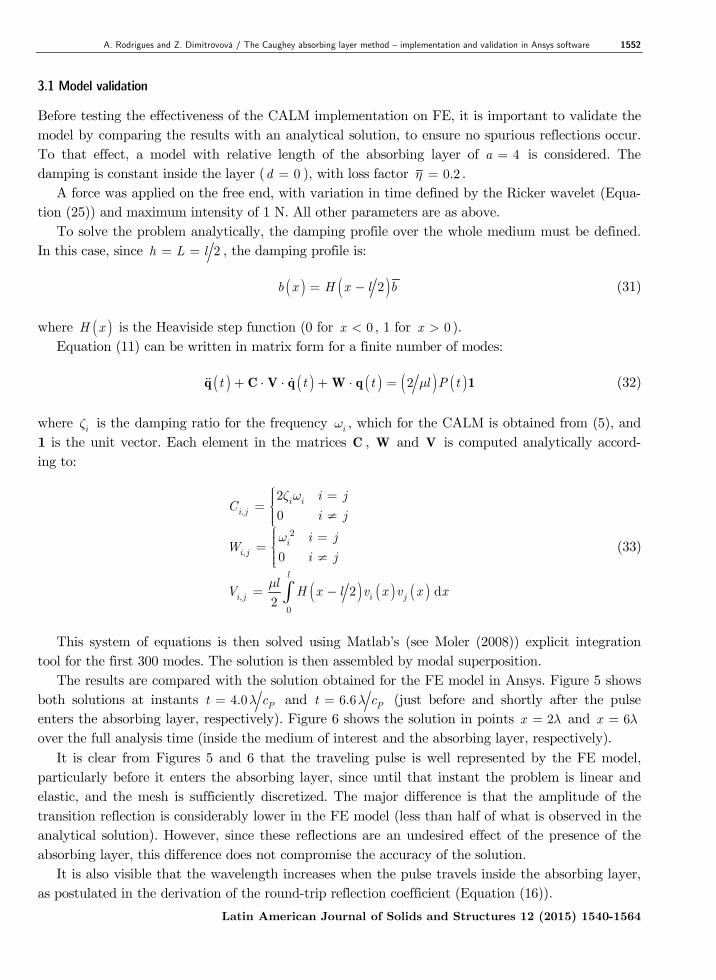
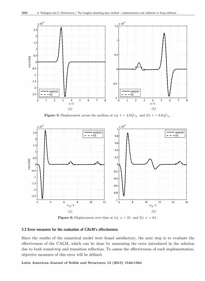
This system of equations is then solved using Matlab’s (see Moler (2008)) explicit integration tool for the first 300 modes. The solution is then assembled by modal superposition. The results are compared with the solution obtained for the FE model in Ansys. Figure 5 shows both solutions at instants 4.0 Pt c and 6.6 Pt c (just before and shortly after the pulse enters the absorbing layer, respectively). Figure 6 shows the solution in points 2x and 6x over the full analysis time (inside the medium of interest and the absorbing layer, respectively). It is clear from Figures 5 and 6 that the traveling pulse is well represented by the FE model, particularly before it enters the absorbing layer, since until that instant the problem is linear and elastic, and the mesh is sufficiently discretized. The major difference is that the amplitude of the transition reflection is considerably lower in the FE model (less than half of what is observed in the analytical solution). However, since these reflections are an undesired effect of the presence of the absorbing layer, this difference does not compromise the accuracy of the solution. It is also visible that the wavelength increases when the pulse travels inside the absorbing layer, as postulated in the derivation of the round-trip reflection coefficient (Equation (16)).



(a) (b)

Figure 5: Displacement across the medium at (a) 4.0 Pt c and (b) 6.6 Pt c .

(a) (b)

Figure 6: Displacement over time at (a) 2x and (b) 6x .

3.2 Error measures for the evaluation of CALM’s effectiveness

Since the results of the numerical model were found satisfactory, the next step is to evaluate the effectiveness of the CALM, which can be done by measuring the error introduced in the solution due to both round-trip and transition reflection. To assess the effectiveness of each implementation, objective measures of this error will be defined.



Three different error measures are considered: the maximum amplitude of the reflected waves, the maximum 2L -norm of the reflected waves and the time integration of the 2L -norm of the re-flected waves. To define any of these error measures, it is necessary to separate the vibrations that are due to the presence of the absorbing layer from the ones that would occur if the medium was truly semi-infinite. Consider the numerical solution inside the medium of interest for the problem with the absorb-ing layer for a given time instant it to be iu . The vector iu contains the displacement at the time-step i for each node inside the medium of interest, but not inside the absorbing layer. The solution for a discretised semi-infinite medium can be approximated if one considers a suffi-ciently long model with no absorbing layer. For the case-study, a model with a total length of 16 is enough to ensure that the waves do not reflect of the Dirichlet boundary for the duration of the analysis ( ft ). If the solution for the long model is i

u , then the displacements due to reflection for the CALM model can be obtained by simple subtraction: , 1,2,...,i i i i m u u u (34)

where m is the time step corresponding to ft . Assuming 1 0t 1 48 4 193 48m a m a (35)

The first error measure is the maximum displacement of the reflected waves, and is analogous to the reflection coefficient discussed in Section 2.2. It can be defined as max 0max , 1,2,...,ii

u U i m u (36)

The maximum L2-norm of the reflected waves is normalized by dividing it by the maximum L2-norm of the waves in the long model: 2 2 2

max max max , 1,2,...,i ii iL L L i m u u (37)

where the L2-norm of a vector is defined as

2 21 2

1

, , , ,n

j nj

L u u u u

u u (38)

Lastly, the time integration of the L2-norm of the reflected waves is similar to Equation (37), but replaces the maximum of the L2-norm by an approximation to the integral of the L2-norm over the time interval from the instant when the wave-front of the Ricker wavelet reaches the interface ( wt ) to the end of the simulation ( ft ), divided by the time range to preserve dimensional consistency. The approximation is simply the sum of the L2-norm for all the time-steps in the range, divided by the number of time steps:



2 22

22 2 2

1d

max max max

f

w

m mt

i if wt i wf w i wt

i i ii i i

tL L m wL t t t t t t t

LL L L

u uu

u u u (39)

where w is the time-step corresponding to the instant wt .

3.3 Parametric optimization of the loss factor

A parametric test is then performed to find the optimum loss factor as a function of a , which var-ies from a 0.25 to a 4 with increment a 0.25. The loss factor at the end of the absorbing layer initially varied from 0.1 to 2 in increments of 0.1. The damping profile also varied: the monomial profile (Equation (19)) was used with d {0,1,2,3} (constant loss factor and linear, quadratic and cubic variation). A fifth profile, proposed by Oskooi et al. (2008), was tested:

1 1 zs z e

(40)

This profile has the property of being C and therefore is smoother than any monomial func-tion, which should reduce transition reflections. The theoretical round-trip reflection coefficient is

2 2.477aRTR e

(41)

which is lower than that of a monomial profile with d 2. The three error measures are computed for each combination of loss factor, damping profile and absorbing layer length. The optimum loss factor ( ) is the one that minimizes the selected error measure for a particular combination of the absorbing layer length and the damping profile. It should be noted that, for very short absorbing layers, the optimum loss factor may not be in the range 0 < < 2. In those cases, the range must be extended to higher values. After determining using 0.1 , a new optimization is performed in the range 0.1 < < 0.1 using 0.01 , which leads to a better approximation of . The results for

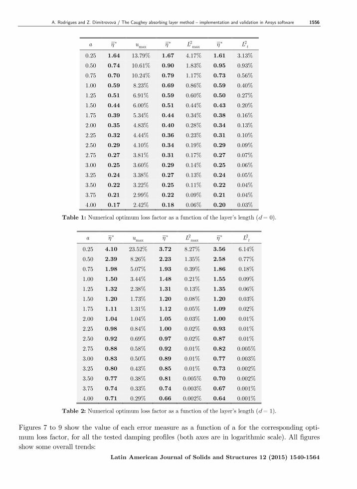
0d (constant loss factor) are summarized in Table 1. The optimum loss factors obtained for each error measure are close to each other, and in par-ticular, the values obtained for maxu and 2

tL are practically the same, save for a few exceptions. Table 2 presents the same information for a linear profile (d 1). It is clear from Table 2 that the error for the linear profile is much lower than that of the con-stant loss factor for any length of the absorbing layer with the exception of a 0.25. It is also evi-dent that the optimum loss factor is considerably higher. This agrees with Equation (20), that shows that higher values of d require higher to keep round-trip reflections low.



a maxu 2maxL 2

tL

0.25 1.64 13.79% 1.67 4.17% 1.61 3.13% 0.50 0.74 10.61% 0.90 1.83% 0.95 0.93% 0.75 0.70 10.24% 0.79 1.17% 0.73 0.56% 1.00 0.59 8.23% 0.69 0.86% 0.59 0.40% 1.25 0.51 6.91% 0.59 0.60% 0.50 0.27% 1.50 0.44 6.00% 0.51 0.44% 0.43 0.20% 1.75 0.39 5.34% 0.44 0.34% 0.38 0.16% 2.00 0.35 4.83% 0.40 0.28% 0.34 0.13% 2.25 0.32 4.44% 0.36 0.23% 0.31 0.10% 2.50 0.29 4.10% 0.34 0.19% 0.29 0.09% 2.75 0.27 3.81% 0.31 0.17% 0.27 0.07% 3.00 0.25 3.60% 0.29 0.14% 0.25 0.06% 3.25 0.24 3.38% 0.27 0.13% 0.24 0.05% 3.50 0.22 3.22% 0.25 0.11% 0.22 0.04% 3.75 0.21 2.99% 0.22 0.09% 0.21 0.04% 4.00 0.17 2.42% 0.18 0.06% 0.20 0.03%

Table 1: Numerical optimum loss factor as a function of the layer’s length (d = 0).

a maxu 2maxL 2

tL

0.25 4.10 23.52% 3.72 8.27% 3.56 6.14% 0.50 2.39 8.26% 2.23 1.35% 2.58 0.77% 0.75 1.98 5.07% 1.93 0.39% 1.86 0.18% 1.00 1.50 3.44% 1.48 0.21% 1.55 0.09% 1.25 1.32 2.38% 1.31 0.13% 1.35 0.06% 1.50 1.20 1.73% 1.20 0.08% 1.20 0.03% 1.75 1.11 1.31% 1.12 0.05% 1.09 0.02% 2.00 1.04 1.04% 1.05 0.03% 1.00 0.01% 2.25 0.98 0.84% 1.00 0.02% 0.93 0.01% 2.50 0.92 0.69% 0.97 0.02% 0.87 0.01% 2.75 0.88 0.58% 0.92 0.01% 0.82 0.005% 3.00 0.83 0.50% 0.89 0.01% 0.77 0.003% 3.25 0.80 0.43% 0.85 0.01% 0.73 0.002% 3.50 0.77 0.38% 0.81 0.005% 0.70 0.002% 3.75 0.74 0.33% 0.74 0.003% 0.67 0.001% 4.00 0.71 0.29% 0.66 0.002% 0.64 0.001%

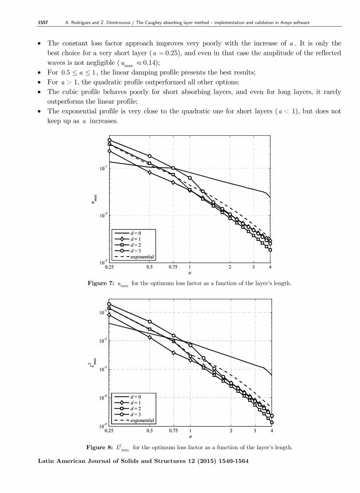
Table 2: Numerical optimum loss factor as a function of the layer’s length (d = 1). Figures 7 to 9 show the value of each error measure as a function of a for the corresponding opti-mum loss factor, for all the tested damping profiles (both axes are in logarithmic scale). All figures show some overall trends:



• The constant loss factor approach improves very poorly with the increase of a . It is only the best choice for a very short layer (a 0.25), and even in that case the amplitude of the reflected waves is not negligible ( maxu 0.14);

• For 0.5 1a , the linear damping profile presents the best results; • For a > 1, the quadratic profile outperformed all other options; • The cubic profile behaves poorly for short absorbing layers, and even for long layers, it rarely

outperforms the linear profile; • The exponential profile is very close to the quadratic one for short layers (a < 1), but does not

keep up as a increases.

Figure 7: maxu for the optimum loss factor as a function of the layer’s length.

Figure 8: 2

maxL for the optimum loss factor as a function of the layer’s length.



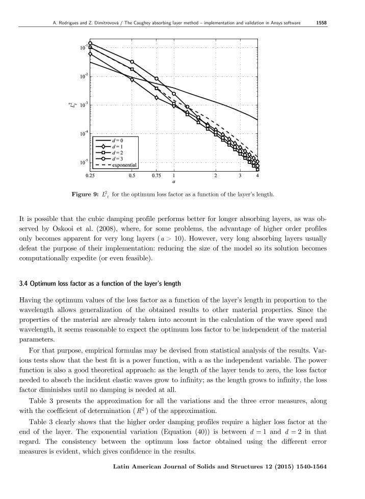
Figure 9: 2

tL for the optimum loss factor as a function of the layer’s length.

It is possible that the cubic damping profile performs better for longer absorbing layers, as was ob-served by Oskooi et al. (2008), where, for some problems, the advantage of higher order profiles only becomes apparent for very long layers (a > 10). However, very long absorbing layers usually defeat the purpose of their implementation: reducing the size of the model so its solution becomes computationally expedite (or even feasible).

3.4 Optimum loss factor as a function of the layer’s length

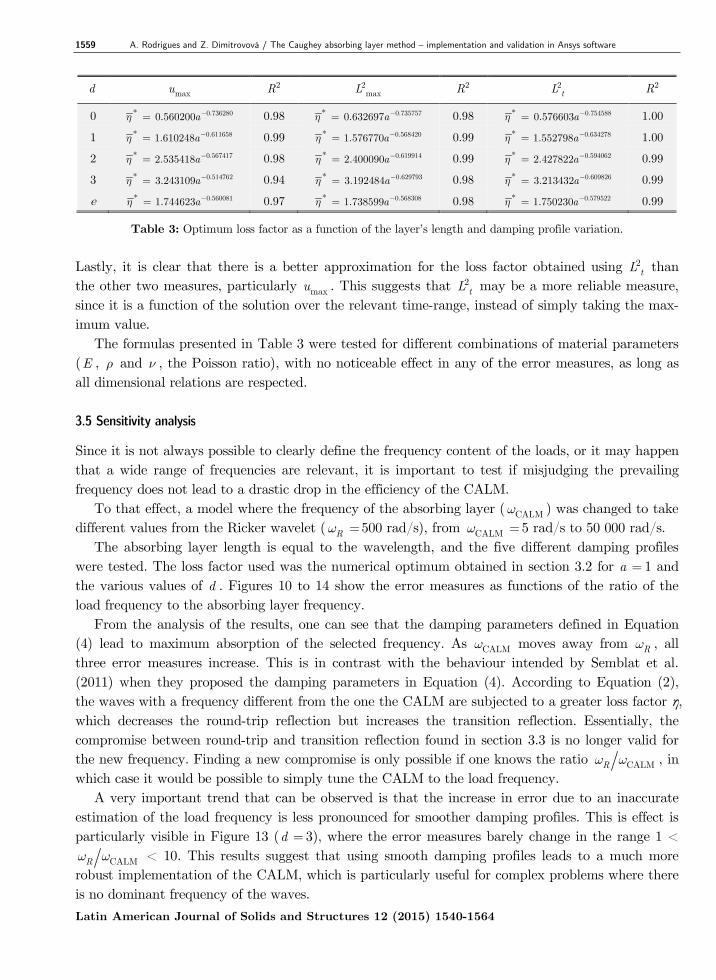
Having the optimum values of the loss factor as a function of the layer’s length in proportion to the wavelength allows generalization of the obtained results to other material properties. Since the properties of the material are already taken into account in the calculation of the wave speed and wavelength, it seems reasonable to expect the optimum loss factor to be independent of the material parameters. For that purpose, empirical formulas may be devised from statistical analysis of the results. Var-ious tests show that the best fit is a power function, with a as the independent variable. The power function is also a good theoretical approach: as the length of the layer tends to zero, the loss factor needed to absorb the incident elastic waves grow to infinity; as the length grows to infinity, the loss factor diminishes until no damping is needed at all. Table 3 presents the approximation for all the variations and the three error measures, along with the coefficient of determination ( 2R ) of the approximation. Table 3 clearly shows that the higher order damping profiles require a higher loss factor at the end of the layer. The exponential variation (Equation (40)) is between d 1 and d 2 in that regard. The consistency between the optimum loss factor obtained using the different error measures is evident, which gives confidence in the results.



d maxu 2R 2maxL 2R 2

tL 2R

0 0.736280* 0.560200a 0.98 0.735757* 0.632697a 0.98 0.754588* 0.576603a 1.00

1 0.611658* 1.610248a 0.99 0.568420* 1.576770a 0.99 0.634278* 1.552798a 1.00

2 0.567417* 2.535418a 0.98 0.619914* 2.400090a 0.99 0.594062* 2.427822a 0.99

3 0.514762* 3.243109a 0.94 0.629793* 3.192484a 0.98 0.609826* 3.213432a 0.99

e 0.560081* 1.744623a 0.97 0.568308* 1.738599a 0.98 0.579522* 1.750230a 0.99

Table 3: Optimum loss factor as a function of the layer’s length and damping profile variation. Lastly, it is clear that there is a better approximation for the loss factor obtained using 2

tL than the other two measures, particularly maxu . This suggests that 2

tL may be a more reliable measure, since it is a function of the solution over the relevant time-range, instead of simply taking the max-imum value. The formulas presented in Table 3 were tested for different combinations of material parameters (E , and , the Poisson ratio), with no noticeable effect in any of the error measures, as long as all dimensional relations are respected. 3.5 Sensitivity analysis

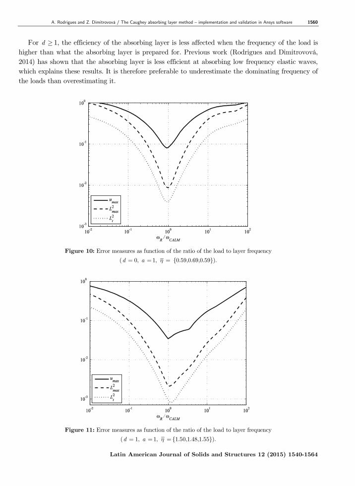
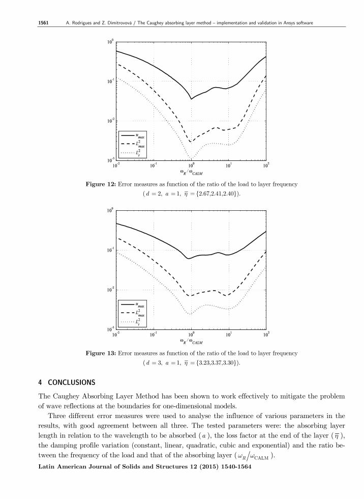
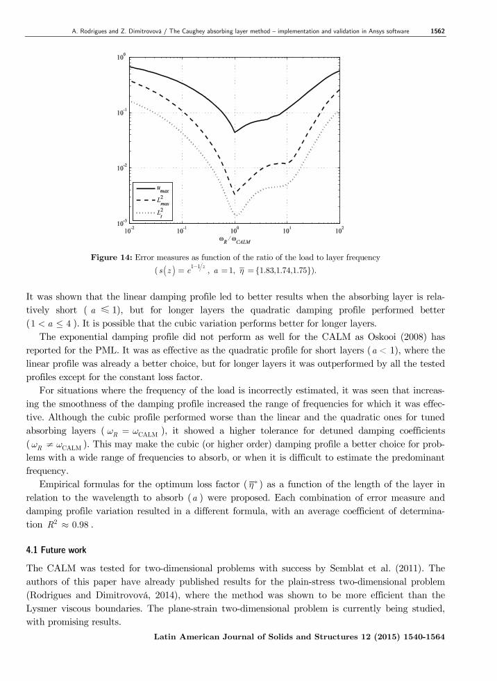
Since it is not always possible to clearly define the frequency content of the loads, or it may happen that a wide range of frequencies are relevant, it is important to test if misjudging the prevailing frequency does not lead to a drastic drop in the efficiency of the CALM. To that effect, a model where the frequency of the absorbing layer ( CALM ) was changed to take different values from the Ricker wavelet ( R 500 rad/s), from CALM 5 rad/s to 50 000 rad/s. The absorbing layer length is equal to the wavelength, and the five different damping profiles were tested. The loss factor used was the numerical optimum obtained in section 3.2 for a 1 and the various values of d . Figures 10 to 14 show the error measures as functions of the ratio of the load frequency to the absorbing layer frequency. From the analysis of the results, one can see that the damping parameters defined in Equation (4) lead to maximum absorption of the selected frequency. As CALM moves away from R , all three error measures increase. This is in contrast with the behaviour intended by Semblat et al. (2011) when they proposed the damping parameters in Equation (4). According to Equation (2), the waves with a frequency different from the one the CALM are subjected to a greater loss factor η, which decreases the round-trip reflection but increases the transition reflection. Essentially, the compromise between round-trip and transition reflection found in section 3.3 is no longer valid for the new frequency. Finding a new compromise is only possible if one knows the ratio CALMR , in which case it would be possible to simply tune the CALM to the load frequency. A very important trend that can be observed is that the increase in error due to an inaccurate estimation of the load frequency is less pronounced for smoother damping profiles. This is effect is particularly visible in Figure 13 (d 3), where the error measures barely change in the range 1 <

CALMR < 10. This results suggest that using smooth damping profiles leads to a much more robust implementation of the CALM, which is particularly useful for complex problems where there is no dominant frequency of the waves. Latin American Journal of Solids and Structures 12 (2015) 1540-1564


For d 1, the efficiency of the absorbing layer is less affected when the frequency of the load is higher than what the absorbing layer is prepared for. Previous work (Rodrigues and Dimitrovová, 2014) has shown that the absorbing layer is less efficient at absorbing low frequency elastic waves, which explains these results. It is therefore preferable to underestimate the dominating frequency of the loads than overestimating it.

Figure 10: Error measures as function of the ratio of the load to layer frequency

(d 0, a 1, {0.59,0.69,0.59}).


(d 1, a 1, {1.50,1.48,1.55}).




(d 2, a 1, {2.67,2.41,2.40}).


(d 3, a 1, {3.23,3.37,3.30}). 4 CONCLUSIONS

The Caughey Absorbing Layer Method has been shown to work effectively to mitigate the problem of wave reflections at the boundaries for one-dimensional models. Three different error measures were used to analyse the influence of various parameters in the results, with good agreement between all three. The tested parameters were: the absorbing layer length in relation to the wavelength to be absorbed (a ), the loss factor at the end of the layer ( ), the damping profile variation (constant, linear, quadratic, cubic and exponential) and the ratio be-tween the frequency of the load and that of the absorbing layer ( CALMR ). Latin American Journal of Solids and Structures 12 (2015) 1540-1564



( 1 1 zs z e

, a 1, {1.83,1.74,1.75}). It was shown that the linear damping profile led to better results when the absorbing layer is rela-tively short ( a ≤ 1), but for longer layers the quadratic damping profile performed better (1 4a ). It is possible that the cubic variation performs better for longer layers. The exponential damping profile did not perform as well for the CALM as Oskooi (2008) has reported for the PML. It was as effective as the quadratic profile for short layers (a < 1), where the linear profile was already a better choice, but for longer layers it was outperformed by all the tested profiles except for the constant loss factor. For situations where the frequency of the load is incorrectly estimated, it was seen that increas-ing the smoothness of the damping profile increased the range of frequencies for which it was effec-tive. Although the cubic profile performed worse than the linear and the quadratic ones for tuned absorbing layers ( CALMR ), it showed a higher tolerance for detuned damping coefficients ( R CALM ). This may make the cubic (or higher order) damping profile a better choice for prob-lems with a wide range of frequencies to absorb, or when it is difficult to estimate the predominant frequency. Empirical formulas for the optimum loss factor ( ) as a function of the length of the layer in relation to the wavelength to absorb (a ) were proposed. Each combination of error measure and damping profile variation resulted in a different formula, with an average coefficient of determina-tion 2 0.98R . 4.1 Future work

The CALM was tested for two-dimensional problems with success by Semblat et al. (2011). The authors of this paper have already published results for the plain-stress two-dimensional problem (Rodrigues and Dimitrovová, 2014), where the method was shown to be more efficient than the Lysmer viscous boundaries. The plane-strain two-dimensional problem is currently being studied, with promising results.



The empirical approximations of the optimum loss factor will be tested in two-dimensional prob-lems, to validate their applicability and verify if they are independent of the properties of the prob-lem (except for the damping profile and length of the absorbing layer in relation to the wavelength). An important development to pursue would be to implement the finite elements with independ-ent Rayleigh damping in the Ansys software, so the method could be applied to more complex problems, including three-dimensional models. Lastly, the theoretical analysis of the CALM must be further developed. In first place, the as-sumption that the decay in amplitude of the reflected waves is minimal for the desired frequency was not verified for the case study. Second, the theoretical prediction of the coefficients of reflection provided a reasonable approximation, but without the accuracy required to propose a theoretical optimum loss factor. Acknowledgements

This work was supported by the Fundação para a Ciência e a Tecnologia (FCT), Portugal, both directly in the form of a PhD grant [SFRH/BD/75375/2010] and through IDMEC, under LAETA, project [UID/EMS/50022/2013]. The authors wish to thank Professor Corneliu Cişmaşiu of the Department of Civil Engineering, Faculdade de Ciências e Tecnologia, Universidade Nova de Lisboa for contributing with his insight about dynamic problems in FEM, particularly during the initial stages of this work. References Banerjee, P.K., Butterfield, R., (1981). Boundary element methods in engineering science. McGraw-Hill Book Co.

Bérenger, J.P., (1994). A perfectly matched layer for the absorption of electromagnetic waves. Journal of Computa-tional Physics 114: 185–200.

Bettess, P., (1977). Infinite elements. International Journal for Numerical Methods in Engineering 11(1): 53–64.

Chapman, C., (2004). Fundamentals of seismic wave propagation. Cambridge University Press.

Chew, W.C., Weedon, W.H., (1994). A 3D perfectly matched medium from modified Maxwell’s equations with stretched coordinates. Microwave and Optical Technology Letters 7(13): 599–604.

Clough, R.W., Penzien, J. ,(1993). Dynamics of structures. McGraw-Hill Education. Engquist, B., Majda, A., (1977). Absorbing boundary conditions for numerical simulation of waves. Proceedings of the National Academy of Sciences 74(5): 1765–1766.

Engquist, B., Majda, A., (1979). Radiation boundary conditions for acoustic and elastic wave calculations. Commu-nications on Pure and Applied Mathematics 32(3): 313–357.

Hallquist, J.O. et al. (2006). LS-DYNA Theory Manual. Livermore Software Technology Corporation.

Holland, R., Williams, J.W., (1983). Total-field versus scattered-field finite-difference codes: A comparative assess-ment. IEEE Transactions on Nuclear Science 30(6): 4583–4588. IEEE.

Hosken, J.W.J., (1988). Ricker wavelets in their various guises. First Break 6(1): 24–33. Hughes, T.J.R., (1987). The finite element method: linear static and dynamic finite element analysis. Prentice-Hall.

Karol, R.H., (1960). Soils and soil engineering. Prentice-Hall.

Katsikadelis, J.T., (2002). Boundary elements: theory and applications. Elsevier Science.

Kohnke, P., (1999). ANSYS theory reference. Ansys.



Lindman, E.L., (1975). “Free-space” boundary conditions for the time dependent wave equation. Journal of Compu-tational Physics 18(1): 66–78.

Liner, C.L., Bodmann, B.G., (2010). The Wolf ramp: reflection characteristics of a transition layer. Geophysics 75(5): 31–35.

Liu, M., Gorman, D.G., (1995). Formulation of Rayleigh damping and its extensions. Computers & Structures 57: 277–285.

Lowrie, W., (2007). Fundamentals of geophysics. Cambridge University Press.

Lysmer, O., Kuhlemeyer, R.L., (1969). Finite dynamic model for infinite media. Journal of the Engineering Mechan-ics Division, ASCE 95: 859–869. Moler, C.B., (2008). Numerical computing with MATLAB. Society for Industrial and Applied Mathematics.

Oskooi, A.F., (2008). An investigation of the perfectly matched layer for inhomogeneous media, Master Thesis, Mas-sachusetts Institute of Technology.

Oskooi, A.F., Zhang, L., Avniel, Y., Johnson, S.G., (2008). The failure of perfectly matched layers, and towards their redemption by adiabatic absorbers. Optics Express 16(15): 11376–11392.

Oskooi, A., Johnson, S.G., (2011). Distinguishing correct from incorrect PML proposals and a corrected unsplit PML for anisotropic, dispersive media. Journal of Computational Physics 230(7): 2369–2377.

Rodrigues, A.F.S., Dimitrovová, Z., (2014). The Caughey Absorbing Layer Method – implementation and validation in Ansys software. 11th World Congress on Computational Mechanics (WCCM XI): 557–568.

Semblat, J.F., Lenti, L., Gandomzadeh, A., (2011). A simple multi-directional absorbing layer method to simulate elastic wave propagation in unbounded domains. International Journal for Numerical Methods in Engineering 85(12): 1543–1563.

Sommerfeld, A., (1949). Partial Differential Equations in Physics (Vol. 1). Academic Press.

Wolf, A., (1937). The reflection of elastic waves from transition layers of variable velocity. Geophysics 2(4): 357–363.


Documents

The Caughey absorbing layer method – implementation … · This paper addresses the Caughey Absorbing Layer Method ... validation in Ansys software . ... a parametric optimization