IZA DP No. 3630

The Causal Effect of Parent’s Schooling on Children’sSchooling: A Comparison of Estimation Methods

Helena HolmlundMikael LindahlErik Plug

DI

SC

US

SI

ON

PA

PE

R S

ER

IE

S

Forschungsinstitutzur Zukunft der ArbeitInstitute for the Studyof Labor

August 2008

The Causal Effect of Parent’s

Schooling on Children’s Schooling: A Comparison of Estimation Methods

Helena Holmlund CEP, London School of Economics

Mikael Lindahl

Uppsala University and IZA

Erik Plug

University of Amsterdam and IZA

Discussion Paper No. 3630 August 2008

IZA

P.O. Box 7240 53072 Bonn

Germany

Phone: +49-228-3894-0 Fax: +49-228-3894-180

E-mail: iza@iza.org

Any opinions expressed here are those of the author(s) and not those of IZA. Research published in this series may include views on policy, but the institute itself takes no institutional policy positions. The Institute for the Study of Labor (IZA) in Bonn is a local and virtual international research center and a place of communication between science, politics and business. IZA is an independent nonprofit organization supported by Deutsche Post World Net. The center is associated with the University of Bonn and offers a stimulating research environment through its international network, workshops and conferences, data service, project support, research visits and doctoral program. IZA engages in (i) original and internationally competitive research in all fields of labor economics, (ii) development of policy concepts, and (iii) dissemination of research results and concepts to the interested public. IZA Discussion Papers often represent preliminary work and are circulated to encourage discussion. Citation of such a paper should account for its provisional character. A revised version may be available directly from the author.

IZA Discussion Paper No. 3630 August 2008

ABSTRACT

The Causal Effect of Parent’s Schooling on Children’s Schooling: A Comparison of Estimation Methods*

Recent studies that aim to estimate the causal link between the education of parents and their children provide evidence that is far from conclusive. This paper explores why. There are a number of possible explanations. One is that these studies rely on different data sources, gathered in different countries at different times. Another one is that these studies use different identification strategies. Three identification strategies that are currently in use rely on: identical twins; adoptees; and instrumental variables. In this paper we apply each of these three strategies to one particular Swedish data set. The purpose is threefold: (i) explain the disparate evidence in the recent literature; (ii) learn more about the quality of each identification procedure; and (iii) get at better perspective about intergenerational effects of education. We find that the three identification strategies all produce intergenerational schooling estimates that are lower than the corresponding OLS estimates, indicating the importance of accounting for ability bias. But interestingly, when applying the three methods to the same data set, we are able to fully replicate the discrepancies across methods found in the previous literature. Our findings therefore indicate that the estimated impact of parental education on that of their child in Sweden does depend on identification, which suggests that country and cohort differences do not lie behind the observed disparities. Finally, we conclude that income is a mechanism linking parent’s and children’s schooling, that can partly explain the diverging results across methods. JEL Classification: I20, J30, J62 Keywords: intergenerational mobility, education, causation, selection, identification Corresponding author: Mikael Lindahl Department of Economics Uppsala University SE-751 20 Uppsala Sweden E-mail: Mikael.Lindahl@nek.su.se

* The authors wish to thank Anders Björklund, Sandra Black, Alan Krueger, Gary Solon, Marianne Sundström, Björn Öckert, and numerous seminar and conference participants in Aarhus, Alicante, Bergen, Brighton, Edinburgh, Gothenburg, Milan, Paris, Princeton, Rotterdam, Tokyo, Trondheim, Verona, Vienna, Warwick for their valuable comments. Thanks also to Valter Hultén for help with the coding of the reform. Financial support from Jan Wallander’s and Tom Hedelius’ foundation, The Swedish Council for Working Life and Social Research (FAS), Berchs and Bergström’s fonder, and the Dutch National Science Foundation [NWO-VIDI45203309] is gratefully acknowledged.

2

1. Introduction

It is widely known that more educated parents get more educated children. For example, in a

literature review published in the Journal of Economic Literature, Bob Haveman and Barbara

Wolfe (1995) conclude that the education of parents is the most fundamental factor in

explaining the child’s success in school. A natural question to raise then is why this is. Is it

because more able parents have more able children? Or is it because more educated parents

have more resources - caused by their higher education - to provide a better environment for

their children to do well in school? We do not know, for two reasons. First, there is not much

evidence available. It is only recently that empirical studies have begun to focus on

establishing a causal relationship between the education of parents and their children. And

second, the few empirical studies on the intergenerational effects of education that are around

tend to reach conflicting conclusions.

To understand why more educated parents have more educated children, it is important

to learn more about the origins of these conflicting results. Is it because most of these studies

rely on different data sources, gathered in different countries at different times? Or is it

because these studies make use of different identification strategies? An answer is not readily

available as there are too many uncertainties. A simple procedure, in which all the available

identification strategies are applied to one particular data set, would help to overcome some of

these uncertainties. Our purpose is to offer the first study that follows this procedure. Three

identification strategies that are currently in use rely on: identical twins; adoptees; and

instrumental variables. In case of the IV-strategy, educational reforms have commonly been

used as instruments for education. We apply and combine each of these three strategies to a

unique Swedish data set.

We think this study deserves the readers’ attention for three reasons. First, this paper

follows naturally from the review of Haveman and Wolfe (1995) (henceforth HW); it surveys

the empirical work done since then, and it replicates and thereby tests the robustness of recent

findings. The latter is important given the limited number of studies available. Second, this

3

paper offers a methodological overview. Each of the three strategies has its own merits,

relying on specific data requirements and identifying assumptions. A comparison between and

combination of three different techniques should lead to a better understanding of the quality

of each identification procedure. And third, this paper should give us a much better

perspective on the underlying mechanisms of intergenerational influences, in particular those

found in Sweden.

Apart from academic reasons, policy makers would like to know whether the

relationship between better educated parents and children is causal or not. A causal

relationship indicates schooling externalities, and may have distributional consequences as

well. If inherited abilities drive the academic success of children in school, then inequality in

opportunity would merely be a reflection of the existing gene pool, leaving scant room for

pro-education policies. If, on the other hand, the parent’s education were primarily

responsible for the child’s success in school, then improving the educational achievement

would not only increase education and reduce the inequality in educational opportunity for

future generations, but also affect their level and distribution of income. Thus, the causal

intergenerational effect of schooling is informative about spill-over effects and indicates a

broad range of returns to educational investments, and the implications for public policy are

therefore huge.

This paper continues as follows. Section 2 briefly surveys the empirical work done

since the review paper of HW. We present studies that focus on causation and not association.

Section 3 sets out the various identification strategies. Section 4 describes our dataset. In

section 5 we replicate, present and compare our parameter estimates to those estimates

reported in previous studies. Our goal here is to produce internally consistent estimates and

compare them to estimates in the literature. In section 6 we deal with issues related to external

consistency: we investigate the role of incomparable samples across methods and whether

intergenerational education effects are non-linear. In section 7, we look at some potentially

important mechanisms explaining the intergenerational transmission process. Section 8

concludes.

4

2. A Review of Recent Empirical Studies

Recent years have seen an upsurge of intergenerational mobility studies that contrast with

earlier efforts and make a distinction between causation and association. Table 1 summarizes

the studies that estimate intergenerational schooling effects and attempt to control for the role

of inherited abilities.

The studies we refer to have been based on three different identification techniques:

twins, adoptees and instrumental variables. Identification in the twins approach comes from

differences in education within pairs of identical twins; the difference in twin parents

education is used to identify effects on their children. The adoption strategy relies on the fact

that there is no genetic transmission from parents to their adopted children. And finally, the

studies adopting instrumental variables take advantage of education reforms where - in our

case - changes in compulsory schooling laws are used to instrument for parental education.

Besides variation among identification methods, another complication in comparing the

findings of different intergenerational mobility studies is the potential variation in estimation

techniques, model and variable specifications, and the choice of control variables in the

model. With respect to estimation techniques and model and variable specifications, the

studies we focus on show little variation. Almost all studies use least squares and regress

school outcomes of children on the same school outcomes of parents, mostly measured by the

number of years of schooling attained. With respect to the choice of control variables in the

model, however, there appears to be less overlap. In particular, there is variation among the

studies in whether or not to include control variables that relate to the age of parents and their

children, and spousal education. We briefly list the main arguments in favour or against

including controls for age and spousal education.

If we begin with age, it is possible that trends in educational attainment interfere with

the estimated intergenerational schooling effects: in Sweden, for example, there has been a

substantial growth in the number of women going to university. In this case, age variables (of

either parent or child) are the natural candidates to include as additional regressors in

5

intergenerational mobility models to obtain detrended estimates. If, on the other hand,

parental schooling has an impact on the timing of childbearing - more schooled mothers are

more likely to postpone motherhood - mobility specifications should not include the age of

both parents and children. Together, these variables define the parent's age at childbirth,

which is endogenous. A common solution to this problem is to run intergenerational mobility

regressions with and without the parental age variables. In most cases the intergenerational

effect estimates appear to be insensitive to the inclusion of parental age variables.

It is also not clear whether one should include spousal education as an additional

explanatory variable. Without the inclusion of the partner’s schooling, the effect of parental

schooling as it is estimated represents both the direct transfer from the given parent and the

indirect transfer from the other parent, which is due to assortative mating effects. Note that if

parents would have randomly met and married, this is not an issue because the inclusion of

the partner’s schooling would have no effect on mobility estimates. With the inclusion of the

partner’s schooling, the estimated transmission effects measure the effect of an increase in a

parent’s schooling on the schooling of his or her child, net of assortative mating effects. The

preferred specification depends, we think, on the (policy) question that is raised or analyzed.

If, for example, we are interested in the schooling of the children, we should not care whether

parental schooling effects run through assortative mating or something else. On the other

hand, if we are interested in the consequences of raising the schooling of mothers but not

fathers, we must quantify assortative mating effects and include the schooling of both parents

simultaneously.1

For most of the studies presented in Table 1, we tabulate the main characteristics of

data sources, identification strategies, relevant model and variable specifications, and the

corresponding mobility estimates. In particular, we report four estimates that aim to measure

the effect of the parent’s education on that of her child: two intergenerational effect estimates

for fathers and mothers that ignore the correlation of educational attainment with unmeasured

1 This may indeed be relevant for policy makers. In Bangladesh, Mexico or Pakistan, for example, there are gender specific programs that aim to raise the schooling of girls but not boys (Paul Schultz 2002; Jere Behrman and Mark Rosenzweig 2005)

6

ability, and two that control for ability transmissions. Some of the studies also aimed to

control for assortative mating effects; if so we include those intergenerational effect estimates

as well.

There are a number of common features of these studies when we consider the

estimates reported in the first two columns. All the estimates indicate that higher parental

education is associated with more years of schooling of own children, and that in most cases

the influence of the mother’s schooling is somewhat larger than that of the father. The results

are, as such, fully in line with those findings reported and summarized in HW. Second, those

studies that control for assortative mating effects indicate that the partial effects of both

parents’ schooling fall, yet always remain positive. It is interesting to see that the partial

schooling effects of both parents are almost always identical, except for Behrman and

Rosenzweig (2002) (henceforth BR) who find that the father’s schooling is the most

important.

But the fundamental problem with interpreting these intergenerational mobility

estimates is that they all ignore the strong correlation of parental schooling with unobserved

ability. Better educated parents are on average better endowed than less educated parents, and

they tend to produce children who do well in school by virtue of better genes. It would be

better to have information on that part of the mother’s and father’s schooling that is

uncontaminated by family genes but still responsible for the school success of future

generations. These estimates are reported in the last two columns.

We begin with the within-twin estimates. Based on monozygotic twin parents from

Minnesota, identical in their endowments including inborn abilities and shared environment

but different in their educational attainment, BR find that the mother’s education has little, if

any a negative impact on the education of her child. Once they look at monozygotic twin

fathers and difference out his endowments that influence their children’s education, the

influence of father’s education remains positive and statistically significant. Kate Antonovics

and Arthur Goldberger (2005) challenge these results, and test the robustness of BR’s findings

to alternative school codings and sample selections. Yet with the twin sample restricted to

7

twins with children 18 years or older, all having finished school, they also produce positive

schooling effects for fathers and no (or much smaller) effects for mothers. In fact, in most of

their alternative samples using various parental schooling measures, within-twin estimates of

maternal schooling effects are lower than those for fathers, which are always positive. Our

conclusion is that the mother’s schooling has little impact on the schooling of her child,

holding everything else (including unobserved ability factors of either mother or father)

constant.

A strategy to account for genetic effects is to use data on adopted children. If adopted

children share only their parents’ environment and not their parents’ genes, any relation

between the schooling of adoptees and their adoptive parents is driven by the influence

parents have on their children’s environment, and not by parents passing on their genes. In the

economics literature, a series of recent papers (Lorraine Dearden, Steve Machin and Howard

Reed 1997; Bruce Sacerdote 2002, 2007; Plug 2004; Anders Björklund, Lindahl and Plug

2004, 2006) have begun to estimate intergenerational schooling effects on samples of parents

and their adopted children. On relatively small samples, the studies of Dearden, Machin and

Reed (1997) and Sacerdote (2002) regress the adopted son’s years of schooling on his

adoptive father’s years of schooling, and report positive and significant effects that are almost

identical to the effects found for fathers and their own-birth sons. They therefore conclude

that background/environment factors are indeed important for intergenerational transmissions.

The other studies that obtain identification from adopted children using much bigger samples

find that the parental effect estimates falls somewhat for fathers but much more so for

mothers, when moving from samples of own birth children to samples of adoptees.

One concern, however, is that in most adoption studies it is difficult to establish a

causal relationship between the schooling of parent and child because of selective placements.

If adoptions are related or if adoption agencies use information on the natural parents to place

children in their adoptive families, the parental schooling estimates possibly pick up selection

effects. Two adoption studies control for this matching correlation. Sacerdote (2007) uses

information on Korean American adoptees who were randomly assigned to adoptive families.

8

Björklund, Lindahl and Plug (2006) (henceforth BLP) use additional information on the

adoptees’ biological parents to control for the impact of selective placements. Both studies

find selection to be important for mothers. Sacerdote (2007) finds that adopted mother’s

education has an impact on the education of the children. BLP find both adoptive (as well as

their biological) parents’ education to be important, even though the impact of the adoptive

mother’s education is very small when education of the spouse is controlled for. The

conclusion from both studies is that parental education has an impact on the education of the

children, even when selective placement is taken into account.

In sum, whether adoptees are raised in Wisconsin, other U.S. states, or Sweden, these

studies always find positive and statistically significant schooling effects when mother’s and

father’s schooling are included as separate regressors. Provided that these models are

correctly specified, the range in which family genes are responsible vary between 15 and 80

percent, and average out at 50 percent. Note that these percentages include assortative mating

effects. When these adoption studies control for assortative mating effects and include

mother’s and father’s schooling simultaneously, they find that mother’s schooling effect is not

bigger but mostly smaller than that of her husband. The bulk of the evidence, thus, indicates

that for the child’s schooling, nurture is indeed an important factor.2 Since these studies also

lend some support to the notion that the nurturing contribution of father’s schooling is

somewhat bigger than that of his wife, these results are in this respect comparable to those

obtained in previous twin studies. However, a difference is that adoption studies generally

find positive effects of mother’s education, at least when the control for spouse’s education is

omitted.

Recent IV studies exploit reforms in the compulsory schooling legislation to identify

the effect of parent’s schooling on their children’s. Black, Devereux and Salvanes (2005)

(henceforth BDS) use changes in compulsory schooling laws introduced in different

Norwegian municipalities at different times during the sixties and early seventies. Because

2 Sacerdote (2000, 2002) and Plug and Wim Vijverberg (2003) focus on nature/nurture decompositions and interpret the difference between own-birth and adoption effects to measure the relative importance of inherited abilities.

9

compulsory schooling increased from seven to nine years, some parents experienced two extra

years of schooling than other parents similar to them on any other point but their year and

municipality of birth. As such, the reform generates exogenous variation in parental schooling

that is independent of endowments. Using the timing of the reform to instrument for parental

schooling, BDS produce mobility estimates that are imprecise and statistically insignificant.

When they restrict the sample to those parents with less than 10 years of education, assuming

that the reform has little bite for those acquiring more than that, their precision increases.

They then find no effect of father’s schooling and a positive but small effect of mother’s

schooling (which is primarily driven by a relationship between young mothers and their sons).

The larger variation in compulsory schooling reforms together with their sample-selection

rule should enable BDS to arrive at more precise estimates than comparable IV studies.3

Arnaud Chevalier (2004), for example, also uses a change in the compulsory schooling law in

Britain in 1957. He finds a large positive effect of mother’s education on her child’s education

but no significant effect of paternal education. Note, however, that a limitation of his study is

that the legislation was implemented nationwide; as a result, there is no cross-sectional

variation in the British compulsory schooling law.

If information on the children’s years of schooling is not available because children are

too young, and still live with their parents, researchers often rely on intermediate schooling

outcomes that are available, such as test scores or grade repetition.4 To date there are three

instrumental variable studies that link the years of schooling of parents to these intermediate

outcomes of children (Philip Oreopoulos, Marriane Page and Ann Huff Stevens 2003, 2006;

Pedro Carneiro, Costas Meghir and Matthias Parey 2007; Eric Maurin and Sandra McNally

2008). We restrict our discussion to grade repetition, which is one of the outcomes these

3 Many empirical studies that make use of comparable compulsory school law changes in the United States, for example, rely on schooling variation across 50 different states. In Norway BDS exploit a much larger source of municipality-variation. The Norwegian reform to increase compulsory schooling from 7 to 9 years was phased across more than 700 municipalities between the years 1959 and 1973. 4 There are different ways to deal with samples in which not all children have finished their schooling. One alternative to intermediate outcomes is to use methods to correct for the censored observations. Monique de Haan and Plug (2006) investigate the consequences of three different methods that deal with censored observations: maximum likelihood approach, replacement of observed with expected years of schooling and elimination of all school-aged children. Of the three methods, the one that treats parental expectations as if they were realizations performs best.

10

studies have in common. The study by Oreopoulos, Page and Stevens (2003) uses U.S.

compulsory schooling reforms, which occurred in different states at different times and finds

that when the mother’s and father’s schooling are included as separate regressors, the

influence of the mother’s and father’s schooling on grade repetition are equally important.5

Results do not change when they use a restricted sample of low-educated parents. This IV

study, and the one by BDS, obtains identification from compulsory schooling extensions and

therefore estimates intergenerational mobility effects among lower educated parents. One

concern could be that parental schooling effects are transmitted differently, and perhaps more

successfully, among higher educated parents. The two remaining studies, by Carneiro, Meghir

and Parey (2007) and Maurin and McNally (2008), address this concern and consider grade

repetition as outcomes but focus on variation in higher education. With instruments that are

very different (county-by-year variation in tuition fees and college location in the U.S. versus

year-by-year variation in the quality of entry exams in French universities), their results

suggest that parental education matters in lowering repetition probabilities.

Most of the IV studies we refer to suffer from two weaknesses. First, most of the

instruments used require identification assumptions/exclusion restrictions that may not hold in

practice. Except for the compulsory schooling instruments in Norway and the U.S., the

instruments used are either statistically weak (tuition fees and college location) or depend too

much on year by year variation, or do not distinguish instrument from cohort variation and are

therefore less convincing (exam quality, U.K. school reforms). Second, it remains unclear

how informative the intermediate outcomes are when it comes to assessing intergenerational

schooling effects. With these weaknesses in mind, we are inclined to take the results of BDS

most seriously.

In sum, we think that all these twin, adoption and IV findings suggest schooling itself is

5 The specification most commonly used in the literature regresses school outcomes of children on years of schooling of mothers, fathers or both. Oreopoulos, Page and Stevens (2006) use the sum of the mother’s and father’s years of schooling as their parental schooling regressor and argue that when mother’s and father’s schooling are included simultaneously to allow for assortative mating effects, their estimates are too imprecise. In their working paper version, however, they do report results without controlling for assortative mating effects. These are the results that we refer to in Table 1.

11

in part responsible for the intergenerational schooling link: more educated parents get more

educated children because of higher education. It is unclear, however, whether it is the

schooling of the mother, the schooling of the father or the schooling of both parents that is the

decisive factor. The estimates in the last two columns of Table 1 appear to be too diverse to

establish one consistent pattern. Recent twin and adoption studies point to the father, whereas

recent IV studies point to the mother as having the strongest impact. Where these differences

come from, we do not know. In the following sections we will focus our attention on finding

possible answers.

3. Causal Modelling of Intergenerational Schooling Effects

To evaluate the empirical studies that attempt to estimate the causal relationship between the

education of parents and their children, we need a methodological framework to clarify and

judge the credibility of the identification methods used. This section provides such a

framework and discusses the implications for estimation. We start with a model of

intergenerational income mobility by Gary Solon (2004), inspired by Gary Becker and Nigel

Tomes (1979, 1986), to understand why the schooling of one generation may matter for the

schooling of the next one, and to arrive at regression equations that are commonly used to

estimate intergenerational associations of schooling. We then continue and discuss how we

(aim to) identify and estimate the causal schooling link between parent and child using

identical twins, adoptees and natural experiments.

3.1 Theoretical Framework

In this particular intergenerational model, we assume that a single parent (p) with one child

(c) spends all of her (lifetime) after-tax income pY on own consumption pC and investment

in her child pM . This implies that

ppp MCY += (1)

12

The child’s schooling cS is assumed to depend linearly on the logarithm of parent’s

investment pM , and some component pN which represents the combination of everything

else the parent provides a child.

ppc NMaS += ln1 (2)

In this schooling production function, the parameter 1a measures the effect of parental

investment on the child’s schooling, where marginal effects fall with increasing investments.

In our model pM is endogenously determined. The other input pN is exogenously determined

and represents ”everything else” that the child receives from his/her parent: pN includes the

parent’s genes ph that are passed on automatically, child-rearing talents pf that contribute

to a better environment for the child to do well in school, and pS , which is included to allow

for intergenerational education transmission channels that do not work through parental

investments. To be clear, child-rearing talents pf are not necessarily inborn, but are given

prior to any educational investments, and are as such unaffected by parental schooling

(although the child-rearing talent itself might influence the investment decision). The

component pS on the other hand, represents a combination of factors that result directly from

parental education, but that do not operate through income. Such factors are for example role

model effects (children seek to attain the educational level of their parents), teaching effects

(more educated parents are more efficient at helping their children with schoolwork) or the

fact that more education might alter parental preferences for education more generally. If we

assume a linear relation, the effortless component pN in (2) can be written as

ppppp fqhqSqN ε+++= 321 , (3)

where 1q , 2q and 3q measure how much of the child’s schooling is determined by parent’s

schooling (through other channels than income), genes and child-rearing talents and where

pε represents a specific idiosyncratic shock. And finally, we assume that income is

determined by the stock of human capital, defined by years of schooling S , heritable

13

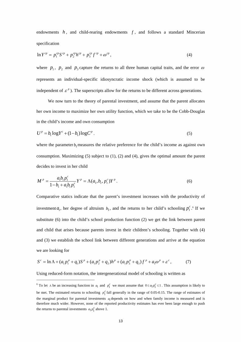
endowments h , and child-rearing endowments f , and follows a standard Mincerian

specification

cpcpcpcpcpcpcpcp fphpSpY ω+++= 321ln , (4)

where 1p , 2p and 3p capture the returns to all three human capital traits, and the error ω

represents an individual-specific idiosyncratic income shock (which is assumed to be

independent of pε ). The superscripts allow for the returns to be different across generations.

We now turn to the theory of parental investment, and assume that the parent allocates

her own income to maximize her own utility function, which we take to be the Cobb-Douglas

in the child’s income and own consumption

pcp CbYbU log)1(log 11 −+= . (5)

where the parameter 1b measures the relative preference for the child’s income as against own

consumption. Maximizing (5) subject to (1), (2) and (4), gives the optimal amount the parent

decides to invest in her child

pcpc

cp YpbaY

pbabpbaM ),,(

1 1111111

111 Λ=+−

= . (6)

Comparative statics indicate that the parent’s investment increases with the productivity of

investment 1a , her degree of altruism 1b , and the returns to her child’s schooling cp1 .6 If we

substitute (6) into the child’s school production function (2) we get the link between parent

and child that arises because parents invest in their children’s schooling. Together with (4)

and (3) we establish the school link between different generations and arrive at the equation

we are looking for

cpppppppc afqpahqpaSqpaS εω ++++++++Λ= 1331221111 )()()(ln , (7)

Using reduced-form notation, the intergenerational model of schooling is written as 6 To let Λ be an increasing function in 1a and cp1 we must assume that 10 11 ≤≤ cpa . This assumption is likely to

be met. The estimated returns to schooling cp1 fall generally in the range of 0.05-0.15. The range of estimates of

the marginal product for parental investments 1a depends on how and when family income is measured and is therefore much wider. However, none of the reported productivity estimates has ever been large enough to push the returns to parental investments cpa 11 above 1.

14

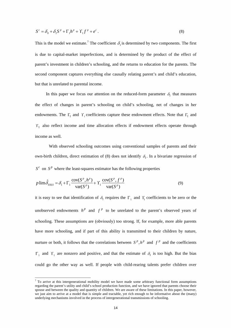
0 1 1 1c p p p cS S h f eδ δ= + + Γ + ϒ + . (8)

This is the model we estimate.7 The coefficient 1δ is determined by two components. The first

is due to capital-market imperfections, and is determined by the product of the effect of

parent’s investment in children’s schooling, and the returns to education for the parents. The

second component captures everything else causally relating parent’s and child’s education,

but that is unrelated to parental income.

In this paper we focus our attention on the reduced-form parameter 1δ that measures

the effect of changes in parent’s schooling on child’s schooling, net of changes in her

endowments. The 1Γ and 1ϒ coefficients capture these endowment effects. Note that 1Γ and

1ϒ also reflect income and time allocation effects if endowment effects operate through

income as well.

With observed schooling outcomes using conventional samples of parents and their

own-birth children, direct estimation of (8) does not identify 1δ . In a bivariate regression of

cS on pS where the least-squares estimator has the following properties

1 1 1 1cov( , ) cov( , )ˆlim

var( ) var( )

p p p p

OLS p p

S h S fpS S

δ δ= +Γ +ϒ (9)

it is easy to see that identification of 1δ requires the 1Γ and 1ϒ coefficients to be zero or the

unobserved endowments ph and pf to be unrelated to the parent’s observed years of

schooling. These assumptions are (obviously) too strong. If, for example, more able parents

have more schooling, and if part of this ability is transmitted to their children by nature,

nurture or both, it follows that the correlations between pp hS , and pf and the coefficients

1Γ and 1ϒ are nonzero and positive, and that the estimate of 1δ is too high. But the bias

could go the other way as well. If people with child-rearing talents prefer children over

7 To arrive at this intergenerational mobility model we have made some arbitrary functional form assumptions regarding the parent’s utility and child’s school production function, and we have ignored that parents choose their spouse and between the quality and quantity of children. We are aware of these limitations. In this paper, however, we just aim to arrive at a model that is simple and tractable, yet rich enough to be informative about the (many) underlying mechanisms involved in the process of intergenerational transmissions of schooling.

15

schooling, and the correlation between schooling and child-rearing endowments is negative it

is also possible that the estimate of 1δ is too low.8 Whether the bias is pushing 1δ up or

downwards is, in the end, an empirical question. One that we aim to pursue in this study.

The previous literature has relied on three alternative identification procedures to

estimate the parameter 1δ : twins, adoptees and instrumental variables. In what follows, we

establish whether each of these methods can give us a consistent estimate of the

intergenerational schooling effect. In this section we focus on those assumptions necessary to

attain internally consistent estimates. Later, in section 6, we discuss those assumptions needed

to generalize the findings to the population of all children. Evaluation of these procedures in

terms of their internal and external validity will help us in comparing the three different

techniques.

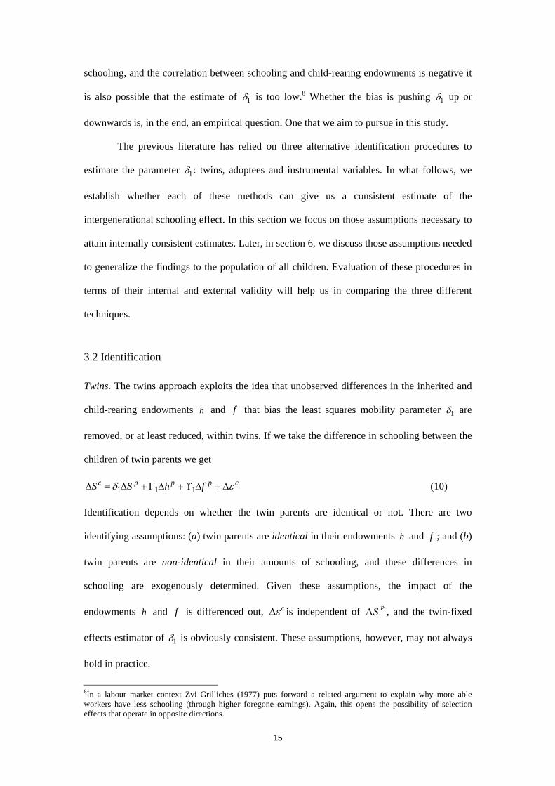
3.2 Identification

Twins. The twins approach exploits the idea that unobserved differences in the inherited and

child-rearing endowments h and f that bias the least squares mobility parameter 1δ are

removed, or at least reduced, within twins. If we take the difference in schooling between the

children of twin parents we get

1 1 1c p p p cS S h fδ εΔ = Δ + Γ Δ + ϒ Δ + Δ (10)

Identification depends on whether the twin parents are identical or not. There are two

identifying assumptions: (a) twin parents are identical in their endowments h and f ; and (b)

twin parents are non-identical in their amounts of schooling, and these differences in

schooling are exogenously determined. Given these assumptions, the impact of the

endowments h and f is differenced out, cεΔ is independent of PSΔ , and the twin-fixed

effects estimator of 1δ is obviously consistent. These assumptions, however, may not always

hold in practice.

8In a labour market context Zvi Grilliches (1977) puts forward a related argument to explain why more able workers have less schooling (through higher foregone earnings). Again, this opens the possibility of selection effects that operate in opposite directions.

16

The first assumption of identical endowments, for example, applies more likely to

monozygotic twins than to dizygotic twins. Monozygotic twins are genetically identical.

Dizygotic twins share on average about 50 percent of their genes. The particular twin sample

used in this study contains both monozygotic and dizygotic twins. This means that without

information on zygosity, some of the inborn endowments remain with differencing, and that

the corresponding selection effect is likely smaller but not eliminated. To assess the

seriousness of the remaining bias, we provide meaningful lower and upper bounds on the true

parameter 1δ by estimating a similar mobility relationship on a sample of closely spaced

same-sex siblings, and then examine different combinations of the twin and sibling estimators

using additional information on the fraction of identical twins in our twin sample. The

derivation of these lower and upper bounds has been relegated to Appendix A.

The second assumption has been called into question too. John Bound and Solon

(1999), for example, emphasize the importance of unobserved heterogeneity in within-

identical-twin estimates for schooling. Since twin identification requires that monozygotic

twins are almost but not exactly identical, they wonder to which extent the forces that led

some identical twins to end up with non-identical amounts of schooling are randomly

determined. If the school differences of twins are endogenously determined, it is possible that

the estimate of 1δ is still biased, even in case the inborn endowments are fully controlled for.

In our model the heterogeneity that remains is represented by that part of pf that is not inborn

but acquired in early childhood and specific to each child. Non-random school differences

occur, for example, when parents treat their twins differently in response to these non-genetic

differences. If one of the twins is, for some unknown reason, more promising than the other,

equity-driven parents may decide to provide additional tutoring to the least promising twin. If,

on the other hand, parents are more efficiency driven, they may choose to invest more in the

schooling of the more promising twin. Depending on whether cεΔ and PSΔ are positively or

negatively correlated, our estimates of 1δ are either upward or downward biased.

There is little empirical evidence that documents the extent to which unobserved

17

heterogeneity among monozygotic twins is random or not. A few papers have considered a

number of plausible candidates. Orley Ashenfelter and Cecilia Rouse (1998) observe that

parents of twins tend to select names that are very similar in sound and/or writing, and argue

that parents find it difficult to treat their twin children in any other way than identically.

Gunnar Isacsson (1999) considers various psychological measures, including the degree of

psychological instability, as potential sources of heterogeneity among Swedish-born

monozygotic twins. In his twin study, however, he finds no effect of emotional instability on

schooling.9 If we assume that this particular measure of emotional stability proxies child-

rearing skills, this measure is most relevant to our paper. And Behrman and Rosenzweig

(2004) report that within-identical-twins differences in schooling correlate strongly with birth-

weight differences in the U.S., and argue that much of the unobserved heterogeneity can be

traced back to non-genetic birth-weight differences. Black, Devereux and Salvanes (2007)

similarly find twin-differences in birth weight to be correlated with twin-differences in

schooling in Norway, and that the magnitude is similar to the cross-sectional estimate.

Dorothe Bonjour et al. (2003) do not find twin-differences in birth weight to be correlated

with twin-differences in schooling, using a sample of U.K. twins. Without information on

birth weights, and without any clear indication of what the unobserved characteristics might

be that make identical twins different, within-twin school differences must be exogenously

determined to draw causal inferences.

Apart from the problem of unobserved heterogeneity within twin parents, there is also

the issue that twin parents are, almost by definition, different from each other because they are

married to different spouses. If both parents, including the twin parent and spouse, shape the

school outcomes of children, this means that the parental school effects as estimated in (10)

will not only capture the impact of the schooling of twin parents but also the impact of the

9 To gain further knowledge on this issue, we are grateful to Gunnar Isacsson for conducting additional analysis on our behalf, using an alternative sample of twins that is more comparable to the one analyzed in this paper. Using a sample of 2,482 female and 2,086 male Swedish MZ twins born 1943-1955, he regressed years of schooling on the psychological instability measure scaled in percentile rank points, controlling for birth year indicators, also including those twins with missing earnings. Using OLS, we find that one standard deviation unit higher score on the psychological instability index, is associated with 0.14-0.15 fewer years of schooling for males-females. And these estimates are statistically significant. Controlling for twin-pair fixed effects, the estimates decrease (to 0.04 and 0.004) and are statistically insignificant.

18

inborn endowments and schooling of their spouses, which are due to assortative mating.

There is some confusion in the literature as to whether we should classify the unobserved

heterogeneity caused by the spouse as bias or not (see discussions in Behrman and

Rosenzweig 2005; Antonovics and Goldberger 2005). Unobserved heterogeneity bias is

absent if we would interpret the within-twin parent estimator inclusive assortative mating

effects. Unobserved heterogeneity bias, however, is present if we would like to estimate

parental schooling effects net of assortative mating effects. It turns out to be difficult to

separate out the influence of the twin parent from the influence of the spouse. The reason is

that potential influences of observed and unobserved characteristics of the spouse (including

schooling and inborn endowments) are not cancelled out in our within-twin regressions. With

spousal schooling included in (10) the within-twin parent estimator would still be biased

upwards if more schooled twin parents marry partners with more favorable endowments.

One other problem that receives much attention is the problem of measurement error. In

fact, the empirical twin literature rather devotes attention to the problem of measurement

error, than to the problem of unobserved heterogeneity. It is well known that random

measurement error biases any estimated effect to zero, and that within-twin differencing likely

amplifies the downward bias. In this particular context, Ashenfelter and Alan Krueger (1994)

warn us that school measures of twins are often measured with error. In this study,

educational classifications are largely drawn from high quality registers, which makes us

believe that measurement error is less of a problem. To test this, however, we are also able to

link part of our register sources to a secondary data set, construct reliability ratios, and correct

our estimates for measurement error bias. In Appendix A we derive a consistent MZ twin

estimator in the case of classical measurement error in schooling without information on

zygosity.

Adoptees. The adoption strategy to identify 1δ exploits the idea that adoptees do not share

their adoptive parents’ genes. If we think of adoption as a natural experiment where babies

19

given up for adoption are randomly placed in their adoptive families, we may either assume

that unobserved heritable endowments of the adoptees’ biological and adoptive parents are

uncorrelated (or that the Γ coefficients are zero). Then for adoptees the schooling function in

(8) is written down as

0 1 1c p p c

iS S fδ δ ε= + + ϒ + (11)

Identification of 1δ now rests on three assumptions: (a) adoptees are randomly assigned to

adoptive families; (b) children are adopted at birth; and (c) the parent’s child-rearing talent

and observed resources are unrelated.10

The first two requirements can arguably be handled for foreign adoptees where the

mechanism of assigning children to their adoptive parents is fairly random. With foreign

adoptions, the absence of genetically related matches is obvious. However, non-random

matches may still occur when adoption agencies have information of the adopted child’s

natural parents. Accessibility, however, is limited, especially for foreign adoptees. We refer to

Appendix B for a detailed description of the institutional details governing the adoption

process in Sweden. Most adoptive parents do not know who the biological parents of their

adopted children are. They know - like we do - the adoptees’ country of origin. In the

empirical adoption analysis we therefore include country/region-of-origin fixed effects.

In the literature, tests have been performed where pre-treatment variables for foreign

adoptees have been regressed on the schooling variables of the adoptive parents. With random

assignment, we should see no relationship between adoptee’s and parent’s characteristics. For

a sample of Korean adoptees adopted by U.S. parents, Sacerdote (2007) finds no evidence of

non-random assignment for pre-treatment variables such as gender of adoptee and age of

adoption. We present additional evidence of this matter by regressing pre-treatment variables

such as gender of adoptee, average economic level in birth country and age of adoption on the

10 Another issue is that children who are given up for adoption, may be different from other children because of the adoption itself. If, for example, indications that adopted children reveal more emotional problems than their class mates – see Michael Bohman (1970) for some Swedish evidence – reflect causal effects of adoption, an outcome like educational attainment might also be affected. As long as these differences are unrelated to the parental schooling, any real adoption effect will not bias our intergenerational adoption estimate. Still this might be more relevant for interpreting the adoption estimates as externally valid. We return to this issue in section 6.

20

schooling of the adoptive parents. Our adoption strategy further requires that children move to

their adoptive parents immediately at birth. We therefore also report estimates from

regressions focussing on foreign adoptees adopted within the first 6 months of their lives.

Intergenerational adoption effects can also be estimated on native-born adoptees. In this

paper we run regressions on a smaller sample of Swedish-born adoptees. These children have

the benefit of being more comparable to non-adopted Swedish children. However, it is less

likely that these children are randomly assigned to adoptive parents. BLP find that schooling

of the biological parents of adoptive children is correlated with schooling of the adoptive

parents. Hence, adoptees born in Sweden in the early 1960s are not randomly placed in their

new families. We also perform some test of this for a sub-sample where we have some

information on biological parent’s characteristics. If there is no association between the

schooling of the adoptive and biological parents, we expect the adoption process to be fairly

random. If the adopted children are genetically related to the adoptive parents our

intergenerational estimations, using Swedish adoptees, will be too high.11 For Swedish

adoptees the adoption age of the children is not recorded. This could bias the intergenerational

estimates in the opposite direction. However, BLP show that Swedish adoptees (at least those

born in the first half of the 1960s) in general are adopted at an early age.

The third assumption requires that the unobserved non-genetic characteristics of the

adoptive parents and the outcome variable are unrelated. This is the only assumption we

cannot handle or test for in any of the adoptive samples. This means that one must (either

assume that pS and pf are independent, or) interpret 1δ as an estimate of the effect on the

adopted child’s schooling of the adoptive parent’s schooling and everything else that is

correlated with the adoptive parent’s schooling and has an independent effect on 1δ , net of the

genetic transmission. We already mentioned that it is not a priori clear whether we should see

this estimate as an upper or lower bound. It depends on whether pf and pS act as

complements or substitutes. Since the adoption strategy does not net out the transmission

11 The intergenerational mobility estimates in BLP are, however, hardly tainted by selective placements.

21

from child-rearing talents pf , we can therefore already at this stage expect that, regardless of

the direction of the bias, adoption estimates should be different from those produced using

twin-fixed effects and instrumental variables.

If we simultaneously want to estimate schooling impacts for both parents,

generalization of the adoption framework is straightforward; we simply add spouse’s

schooling to equation (11). The bias caused by both parents’ heritable endowments is then

eliminated. The inborn child-rearing talents of both adoptive parents, however, still remain. If

better educated parents choose their marriage partner for his/her parenting skills, any bias due

to unobserved parenting skill is then exacerbated.

The compulsory school reform as an instrument. The third strategy considers multi-

generational information that does not rely on twins or adopted children but identifies

intergenerational schooling effects using an instrumental variable approach. We estimate the

effect of parental schooling on child’s schooling by exploiting a reform in compulsory

schooling laws in Sweden during the fifties and early sixties to draw causal inferences. This

reform extended compulsory schooling uniformly to nine years. Before the reform

compulsory schooling took seven years in some municipalities while eight years in others. We

are unable to make a distinction between the two types. The reform was cohort- and

municipality-specific, and was implemented in different municipalities at different times. So

the idea is fairly simple. Since the reform determined whether or not an individual attended

the “old” or “new” compulsory school, some parents experienced one or two extra years of

schooling than other parents similar to them on any other point but their birth year, and

municipality of residence. These discontinuities are then used to identify the causal effect of

parental schooling on child schooling. Appendix B describes the compulsory school reform in

more detail.

For the IV strategy, the empirical counterpart of our model boils down to the following

two equations:

22

0 1c p p c

XS S X eδ δ δ= + + + (12)

'0 1

p p p pXS REFORM X eγ γ δ= + + + (13)

pX is a vector of covariates that includes sets of year-of-birth and municipality-of-residence

dummies (sometimes interacted with a time trend) of the parent, and, for simplicity, we let the

heritable component ph and the child-rearing component pf be included in the error term

ce in equation (12). PREFORM is an indicator that takes the value one if the parent belongs

to a birth cohort that was subject to extended compulsory schooling in the particular

municipality, and zero otherwise. The empirical model is estimated using two stage least

squares, where (13) serves as the first stage using pREFORM as the instrumental variable.

The resulting estimate of 1δ therefore estimates, conditional on covariates, the impact of

parent’s schooling on the schooling of the child using only the part of the variation in parent’s

schooling generated by the reform. This strategy is the one we apply in this paper, and it is the

same as in BDS, on Norwegian data, and as in Oreopoulos, Page and Stevens (2003, 2006),

on U.S. data, although the latter study uses grade repetition for the child as the outcome

variable.

Any identification using instrumental variable techniques depends on the quality of the

instrument. To get an internally consistent estimate of 1δ using 2SLS on (12) and (13), we

need two assumptions to be fulfilled: (a) pREFORM has to be uncorrelated with ce and (b)

pREFORM has to be correlated with parental schooling. Both assumptions need to hold

conditional on all the included covariates. In other words, we need the compulsory school

reform to exert variation in parental schooling that is independent of the parental endowments

ph and pf and of remaining factors in ce , conditional on cohort and municipality indicators.

For (a) to hold, municipality fixed effects likely need to be included, since the pREFORM -

indicator may pick up the tendency that better schooled municipalities were more or less

eager to implement the reform early. Then, identification only requires that unobserved

characteristics of municipalities in equation (12) do not vary systematically during the reform

23

period, and if they do, these changes should be unrelated to the implementation of the reform.

If the implementation of the reform is correlated with changing unobserved characteristics of

municipalities in equation (12), one can attempt to deal with this by also adding municipality-

fixed effects interacted with a linear time trend. This extended model will allow for any

difference in trends in unobservable variables being correlated with reform implementation,

as long as these trends are linear. To avoid problems with weak instruments we require 1γ , the

impact of the reform on parental schooling, to be very precisely estimated.

Is the inclusion of municipality-fixed effects (with or without trend interactions)

sufficient to assure that assumption (a) holds? There are several threats to consistency: Our

IV-estimates are too high if the reform has an independent positive effect on adult outcomes

(and therefore children’s outcomes), conditional on parent’s schooling. A reason for this

could be other simultaneous changes to the education system, as emphasized by Meghir and

Mårten Palme (2005), in estimating earnings effects of this reform. The Swedish compulsory

school reform implied not only two additional years in school, but also affected the

curriculum and the timing of ability tracking. The postponement of tracking might imply

changes in peer group composition, or have consequences for spousal matching. However,

investigating this issue, Holmlund (2007b) finds no effect of the reform on assortative mating.

The issue of simultaneous changes to the education system, and whether such changes

have independent effects on outcomes holding education constant, is of a general concern to

the literature using educational reforms in an instrumental variables setting. The

postponement of ability tracking is in fact common to most Scandinavian compulsory

schooling reforms. And it is likely that expansion of compulsory education, whether in U.S.

states or in Europe, also affects the demand for teachers and has implications for teacher

quality. Any of these effects accompanying changes in the compulsory schooling legislation

is a potential threat to consistency of the IV estimates in the literature.

An additional pitfall takes the form of selective mobility. Since we identify reform

individuals based on the municipality-of-residence in 1960 (65), it is possible that selective

24

mobility prior to that will bias our intergenerational estimates. If reform schools were thought

to be of lower quality, it is possible that parents who prefer non-reform schools over reform

schools decide to move away from reform school areas. Hence, the composition of individuals

in reform municipalities is no longer comparable to that in non-reform areas. Meghir and

Palme (2003) investigate selective mobility using complementary information on birth

municipality, in order to identify movers. They find that 4.3 percent of their sample moved

from a reform-municipality to a municipality not affected for the particular cohort, and that

the mobility in the other direction was of similar magnitude. These findings are confirmed in

Holmlund (2007a). In both these studies, there is also evidence that high (grand-) paternal

education is associated with a higher probability to move from a reform to a non-reform

municipality. However, mobility rates are relatively low, and Meghir and Palme (2003) find

that conditional on observables, living in a reform-municipality cannot predict moving to a

non-reform region. They also find that their results are stable if they exclude the movers from

their empirical analysis. Thus, we cannot rule out bias due to selective mobility, but conclude

that since mobility was very limited, any bias should be small.

For the above reasons one need to be careful in interpreting the IV-estimate as the

causal effect of an additional year of parental schooling. What we can do is to investigate the

sensitivity of our estimates by adding important exogenous variables to our 2SLS

specifications. We therefore add controls for grand-mothers’ and grand-fathers’ education.

Grand-parents’ education is very strongly associated with both parent’s and children’s

education, and should therefore provide a good check of the validity of the IV-estimates.

If we restrict the sample to only those individuals with the lowest level of education, as

in BDS where the sample was restricted to those parents with less than 10 years of schooling

in the main estimations, we need to assume that the reform had no effect on the probability of

attaining post-compulsory schooling. If this assumption does not hold, the composition of

individuals in a municipality will differ pre- and post-reform. This means that those

individuals who gained the most from the reform (and continued their education longer than

what was required) will be excluded. This will likely bias the intergenerational estimate for

25

such a restricted sample downwards. Such spill-over effects can be tested for directly, by

regressing the probability of attaining post-compulsory education on the reform indicator.

An additional source of heterogeneity stems from education and unobservable

characteristics of the spouse. Adding spouse’s years of schooling, treating it as an additional

endogenous variable, we need to use the compulsory schooling reform for the spouse as an

additional instrument. The corresponding empirical specification that in the IV estimation

controls for education of the spouse, will thus instrument each parents’ education with the

parent-specific reform dummy. If many parents and spouses are close in age and from the

same municipality, and there is little variation in reform status of parent and spouse, estimates

may be imprecise. Investigating the effect of the reform on assortative mating, Holmlund

(2007b) finds no evidence of such effects to be important.

As a final remark, the twin-, adoption- and IV-estimators control for different degrees

of child-rearing endowments. A valid IV-strategy nets out the transmission from all

endowments, including child-rearing talents pf . The twin strategy does control for child-

rearing endowments that are shared among twins, but leaves those endowments that are child-

specific untreated. The adoption strategy can only control for child-rearing talents by

assumption. We therefore expect IV-estimates to be different from those produced using twin-

fixed effects and adoptive families.

4. The Swedish data set

We use a very large data set compiled from several different Swedish registers, administered

by Statistics Sweden. We start out with a 35 percent random sample of each cohort born in

Sweden in 1932-1967. By means of population registers, we are able to identify and match

the parents, siblings and children (both biological and adopted) to the sampled individuals.

We use the bi-decennial censuses in 1960-1990 to gather family background information of

the individuals in the random sample, and to identify municipality of residence. In the

censuses, we are also able to track the cohabiting partner of the individuals in the random

26

sample; given that the individuals have children, the censuses provide information on both

parents of the child. However, while we know that the sampled individual is the biological

parent of the child, we do not know whether the partner that we trace in the census is the

biological parent.

Our main variable of interest in this study, years of schooling, is created using the

information in the education register. The education register contains detailed information on

completed level of education. For children, we measure attained education levels in December

2006 (or earlier if education is missing at this time due to emigration or death). We measure

parental education earlier, in December 1990, when the parental cohorts are 35 years of age or

older. In case parental education is missing in the 1990 register, information from later

registers is used.12 The information in the education register of completed level of education is

translated into years of schooling in the following way: 7 for (old) primary school, 9 for (new)

compulsory schooling, 9.5 for (old) post-primary school (realskola), 11 for short high school,

12 for long high school, 14 for short university, 15.5 for long university, and 19 for a PhD

university education. In order for the children to have completed their schooling, we focus on

children that are 23 years of age and older and hence require them to be born 1983 or earlier

to be included in the sample.

We restrict our random sample of parents to married or cohabiting individuals with a

biological (or adopted) child. We also require that their children live with the parents in a

census when they are 6-10 years old.

For the purposes of this study, we constrain the sample to the cohorts born in 1943-

1955. These cohorts were affected by the compulsory schooling reform that was implemented

gradually across Swedish municipalities in the 1950s and 1960s, and to these cohorts it is

possible to match information on whether they were affected by the reform or not. We assign

individuals to the reform based on their year of birth and their municipality of residence at age

10-17 (which we obtain from the 1960 and 1965 censuses). We exclude those cohorts born

12 For the older parental cohorts, the education information we use is constructed by Statistics Sweden using information directly from educational institutions, complemented with answers to detailed questions in censuses 1970 and 1990.

27

prior to 1943 for which the information on municipality of residence might not represent the

municipality in which the individual went to school. We also exclude those municipalities for

which a clear-cut implementation year cannot be determined because the reform was

implemented gradually within the municipality.13

For our two other identification strategies, we compile data sets also based on the

random sample of the 1943-1955 cohorts. An adoption code tells us whether the child is

adopted. We require that the adoptees were adopted by two parents born in Sweden. For

foreign adoptees, we have information on the date of birth and date of immigration of the

adopted child, which makes it possible for us to approximate age of adoption. We further have

information on the child’s native country. We also use a smaller sample of Swedish-born

adoptees. For the Swedish adoptees we have information on the characteristics of the

biological mother for more than half of the sample, and for the biological father for almost

one third of the sample.

We construct the sample of twins in the following way: From the random sample and

their siblings we single out those full biological siblings that are born in the same year and

month. It is not possible to separate monozygotic (MZ) from dizygotic (DZ) twins. However,

by using only same-sex twins we know that about half of the twin sample will consist of MZ

twins. Of the two twins, we require each to have at least one biological child. We assume that

the spouses of each twin are the biological parents of the twin’s children. In the sensitivity

analysis we also focus on closely spaced siblings and select full biological siblings that are

born within 2 years of the randomly sampled individual.

Table 2 reports descriptive statistics for the samples used in this study. In the first two

columns we show means and standard deviations for a 35 percent random sample of married

or cohabiting Swedish individuals, born 1943-55, with at least one child (born no later than

1983). This sample has no further restrictions as compared to the ones we use in our analysis;

in remaining columns we show our data for the twins-, adoptee- and IV-samples. We have

13 Note, however, that although the implementation was gradual within the three big cities Stockholm, Gothenburg and Malmö, we are able to use a more detailed regional coding on parish level in order to keep the cities in the sample. See Holmlund (2007a) for a detailed description of how the reform coding has been constructed.

28

more than 9947 children with same-sex twin parents; 59 percent of them mothers. We see that

twin mothers have on average about half a year less schooling than women in the random

sample.14 Other characteristics are quite similar though. Interestingly, 51 percent of the

children belong to a twin-parent pair with different levels of education. Our adoptive sample

consists of Swedish-born as well as foreign-born adoptees. All-in-all, 69 countries are

represented. The most frequent adoption countries are India (19%), South Korea (19%), and

Sri Lanka (11%). Adoptive parents are better educated than the average parent, yet their

adoptive children complete somewhat less education than the typical child. Adoptive children

are also younger than average.

An interesting group of foreign adoptees are those adopted from South Korea. The

adopted Korean children have more than one year of additional schooling compared to

Swedish-born adoptees, even though there is no difference in parental schooling between

these two groups. Korean babies also complete significantly more schooling than children

adopted from abroad but from other countries, despite that their adoptive parents have less

schooling, on average. Hence, children adopted from South Korea are more successful than

other adoptees and equally successful compared to non-adopted Swedish born children. These

descriptive statistics are in line with other sources indicating that adoptees born in South

Korea constitute a less disadvantaged group among all foreign-born adoptees (Wun-Jung

Kim, 1995; Frank Lindblad, 2004). Pre-and post-natal care is of a very high standard in South

Korea, which means that we can expect Korean babies to be less harmed by their pre-adoption

environment, compared to other foreign-born adoptees in Korea. Also, Korean mothers giving

up their children for adoption are typically from less disadvantaged backgrounds. Our

conclusion is that Korean adoptees form a group that is more comparable to non-adoptees,

than what is the case for most other foreign-born adoptees, who to a higher degree are

represented by disadvantaged children.

The IV sample is smaller than the random sample. Two reasons explain why about 12

14 This might be explained by twins having lower birth weight than non-twins, since studies have found low birth weight to generate worse adult outcomes (see Behrman and Rosenzweig (2004) and Black, Devereux and Salvanes (2007) for two recent studies).

29

percent of the random sample is not present in the current IV sample: (1) we had to exclude

some individuals residing in municipalities where no reliable information on reform year were

to be found, and (2) we also choose to exclude individuals in those municipalities where the

reform was already introduced prior to 1943.15 Also, despite some clear differences, there are

clearly a lot of overlaps in the variable distributions for all the samples.

5. Results

We start out by presenting OLS results using the random sample of the 1943-1955 cohorts.

We regress the education of the child on the education of parents, and the results are reported

in Table 3. Column 1 presents results for mothers and column 2 for fathers. Panel A shows

results using only one parent and panel B shows estimates from regressions controlling for the

education of the spouse. All specifications include controls for the gender of the child and the

parent’s year of birth. The estimates including spouse’s education also control for spouse’s

year of birth. We find that the estimate is 0.28 for mother’s education and 0.23 for father’s

education. When we also control for spouse’s education (panel B), the estimates decrease to

0.20 for mothers and 0.15 for fathers. This reduction is due to assortative mating. These

results are very much in line with earlier results for Sweden (see BLP). These results are our

baseline OLS estimates, to be compared with the corresponding OLS estimates of our twin,

adoptee and IV samples.

Table 3 also presents OLS results including a squared term of parental years of

schooling (see panel C). The coefficients indicate that the intergenerational association in

education is convex; the relationship between parental and child’s education is stronger higher

up in the distribution. If we use the estimates and predict intergenerational coefficients at the

bottom of the educational distribution (7 years of schooling; pre-reform primary schooling)

and at the top (16 years of schooling; long university education), we find clear evidence of

very different returns across the distribution: at the bottom we get 0.16 for mothers and 0.12 15Although, as previously mentioned, for the big cities Stockholm, Gothenburg and Malmö, we have only excluded the parts of the cities that introduced the reform prior to the 1943 cohort.

30

for fathers, and at the top 0.41 for mothers and 0.37 for fathers. We return to the issue of non-

linear effects in section 6.2.

5.1 Twins

Basic results. We now turn to regressing the education of the child on the education of parents

using the sample of twins. As a comparison, we also present results for a sample of all

siblings, and a sample of closely spaced siblings (where the sibling of the parent is born

within ±2 years of the randomly sampled parent). The twin estimates are reported in panel A

of Table 4, and the sibling estimates are shown in panels B and C of the same table. In the

first two columns we show results for mothers and in the last two columns results for fathers.

We report first the cross-sectional intergenerational estimate on each sample, and then turn to

the difference estimates, which identify the intergenerational schooling effects by using

within-family variation. The first row of each panel shows results using only the twin/sibling

parent and the second row shows estimates from regressions controlling for the years of

schooling of the spouse.

The cross-sectional estimates using twins (panel A) reveal that one more year of

schooling for the mother (father) is associated with 0.25 (0.21) more years of schooling for

the child, on average. When we include a control for spouse’s education, the estimates

decrease to about 0.15 (0.17) for fathers (mothers). We note that the intergenerational OLS

estimates using the sample of twins are slightly lower than those using the random sample

(panels A and B of Table 3).

In columns 2 and 4 we apply the twins approach, i.e., we estimate the intergenerational

relationship between twin-parents and their children (who are also cousins), controlling for

twin-pair fixed effects. Hence, we associate the educational differences between cousins with

that of their twin parents. We see that introducing the family-fixed effect reduces the

schooling transmission coefficients, compared to the cross-sectional point estimates, and more

so for mothers than for fathers. The fixed-effect coefficients for mothers and fathers are 0.06

and 0.12, respectively. Moving to the second row, where controls for education of the spouse

31

are included, the schooling effects are reduced to 0.04 for women and 0.11 for men. The

estimate of mother’s schooling, when controlling for spouse’s schooling, is the only

statistically insignificant estimate. The results from the twin-fixed effects estimation show

that mother’s education is no more than half as important as father’s education in the

intergenerational process.

Turning now to the results using the sibling sample (panel B), the assumption that

education is unrelated to inherited abilities within a pair of siblings is less plausible. The

cross-sectional estimates reveal intergenerational schooling effects that are almost identical to

those using the random sample, and very similar to those using the twins sample. In columns

2 and 4 of panel B we control for sibling-fixed effects. We find that the effect of mother’s

education on that of her child is 0.14 without and 0.11 with the control for her husband’s

education. The effect of father’s education is very similar in magnitude: 0.13 and 0.10 without

or with the inclusion of the education of his partner.16 Turning to the results for the closely

spaced sibling sample (panel C), we have eliminated more than 85 percent of all siblings.

Still, the estimates are very similar to the sample of all siblings. However, in order to interpret

these effects as causal, the allocation of education to siblings within the same family should

be exogenous; an assumption too strong to be valid.

Sensitivity analysis. We should keep in mind, however, that the twin estimates presented here

are based on a twin sample containing both MZ and DZ twins, and that no correction has been

made for possible measurement error in parental schooling. As we argue in Appendix A,

under some distributional assumptions about non-twin siblings and twins, we can combine

sibling estimates and twin estimates to either net out any bias caused by the inclusion of DZ

twins in our sample, or place bounds on parental schooling effects. For this purpose we use

the estimates from the regressions using the sample of closely spaced siblings, where we

16 Sibling-fixed effects estimates are also reported in Sandra Black, Paul Devereux and Kjell Salvanes (2003) using a representative sample of Norwegian siblings born between 1947 and 1958 with children who are 20 or older in the year 2000. They find that their fixed-effects estimates are similar for mothers and fathers, positive and statistically significant, yet uniformly lower than their OLS estimates.

32

believe these assumptions are more likely to be met. Let us start by assuming that there is no

measurement error in parental schooling, that twins and siblings are treated very similarly,

and that the intergenerational mobility model as depicted in equation (8) is identical for

siblings and twins. In this case, we identify parental schooling effects as follows:

1 1 1 1ˆ ˆ ˆ2TS TW SIBδ δ δ δ= − = (14)

Our results in Table 4 show that for men, the sibling estimates are similar to the twin

estimates, which means that when we assume that the fraction of DZ twins in our sample of

same-sex twins is equal to 0.5, the consistent estimate of 1δ is similar to the one obtained for

the twin sample. The calculated estimate (standard error) is 0.101 (0.061) without controlling

for spouse’s education. For mothers, the estimate decreases more. It is calculated as -0.004

(0.057) without controlling for spouse’s education. If we also condition on spouse’s education

the numbers are 0.111 for fathers and -0.014 for mothers. Thus had we been able to identify

MZ twins in our sample of twins, our estimates would have been very similar to the current

ones for fathers, and very close to zero for mothers.

Note that if twins are treated more similarly than non-twin brothers and sisters, the

above combination of twin and sibling estimates must be interpreted as a lower bound. Recall

that our twin estimates are flawed as well, and likely produce upper bounds. Taken together,

this means that the intergenerational schooling effects we estimate move somewhere between

-0.01 and 0.06 for mothers, and between 0.10 and 0.12 for fathers (with and without

assortative mating effects). Our results remain practically unchanged: positive effects for

fathers, and almost no effects for mothers.

So what happens if we allow for measurement error in parental schooling? Since we

have register data on educational classifications, we believe that measurement error is less of

a problem. However we still want to test for this. When we calculate the cross sectional

reliability ratios for twins and siblings, using a data set with one survey and one register

measure of schooling, we get the following estimates (standard errors) of reliability ratios for

the register measure: 0.96 (0.04) for fathers and 0.95 (0.04) for mothers. These are much

33

higher than what is typically found in the literature using survey measures. When we consider

school differences between twins and siblings, the reliability ratios decrease as expected to

0.88 for twins and 0.90-0.91 for siblings.

The estimates (standard errors) adjusted for measurement error in parental schooling as

well as correcting for a mixture of DZ and MZ twins are -0.001 (0.065) for mothers and 0.120

(0.069) for fathers. Thus, we conclude that had we been able to identify and use only MZ

twins, and were there no measurement error in the parental schooling variable, our analysis

would have produced causal intergenerational estimates that are similar for fathers, and

smaller for mothers, compared to our baseline twin estimates (reported in Table 4).

Conclusions. To sum up our results based on twin differences, we find that father’s years of

schooling has a positive and significant effect on his child’s years of schooling. For mothers,

we find smaller effects. When we attempt to correct for our sample being a mixture of DZ and

MZ twins and for attenuation bias due to measurement error in parent’s schooling, we find

that estimates using only MZ twins would likely have generated a similar effect for fathers,

but no effect for mothers. When we compare these results to those found previously in the

literature two issues come up. First, an advantage is that our twin sample is much larger than

the one used by BR and Antonovics and Goldberger (2005). Hence, our effects are much

more precisely estimated. Second, a disadvantage is that we cannot distinguish between DZ

and MZ twins. Our twin estimates for fathers are smaller than those previously found, but that

the striking difference between mothers and fathers remains.

5.2 Adoptees

Basic results. Table 5 reports intergenerational education estimates for adoptees and their

adoptive parents. The first three columns present results for mothers and columns 4-6 report

results for fathers. In panel A we do not put any restrictions on adoption age of the child and

make no attempt to control for non-random matching of adoptees to families. In panel B we

34

do. With respect to age of adoption, we do not impose age restrictions for Swedish adoptees

because we cannot observe their adoption age. For foreign adoptees we require them to be

adopted no later than at six months of age. With respect to selective placement of adoptees we

control for the biological characteristics of the biological parents of the adoptive children born

in Sweden. For foreign-born adoptees we do not only control for adoption age, but also

include additional selection characteristics like country/region-of-birth of the child and the

logarithm of GDP per capita in the child’s country of birth.

The structure of Table 5 is as follows. In the first row we present estimates of separate

regressions using the mothers and fathers of the adoptees. In the second row we present

estimates from regressions including both father’s and mother’s education. We use the same

sample in both panels, i.e., we require the adoptive parent we focus on to be born in 1943-55,

whereas the other adoptive parent (the spouse) is not required to be born within this time

period. We show results for Swedish-born adoptees in columns 1 and 4, for foreign-born

adoptees in columns 2 and 5, and for Korean-born adoptees in columns 3 and 6. All

regressions include individual controls for the gender of the child and parent’s year of birth.

We start with Panel A, where we show results for unrestricted samples, including only

a minimum number of control variables. Turning first to estimates for mothers, we see that for

the sample of Swedish-born adoptees, the estimates are positive, without and with controls for

spouse’s education. An additional year of education for mothers is associated with 0.09-0.11

more years for the child. The estimate is somewhat lower when we control for spouse’s

education. We then turn to the estimates for foreign-born adopted children. We find that the

estimated effects are small but statistically significant for mothers, without controlling for the

other parent’s education. An additional year of parental education is associated with 0.02

more years of education for the child.17 For Korean adoptees, the maternal effect is never

statistically significant. Sacerdote (2007) found larger effects for mothers.

If we focus on the estimates for fathers, we see that for Swedish adoptees the estimates

17 Note that adding country/region-of-birth indicators to the specifications using foreign-born adoptees increased estimates by roughly 50 percent. Adding the controls for adoption age and the logarithm of GDP had no further impact on the estimates (although R-squared increases somewhat).

35

are positive, but somewhat lower than for mothers. When we control for spouse’s education,

the estimates decrease slightly and become statistically insignificant. The intergenerational

effect for fathers is estimated to be about 0.03-0.06 for Swedish adoptees. If we instead look

at foreign-born adoptees, estimates are similar to those of mothers. When we control for

spouse’s education, the estimate for all foreign-born adoptees is cut in half and is no longer

significant.

We show the results for the restricted samples using additional control variables in

panel B of Table 5. Starting again with results for mothers, we find that for Swedish-born

adoptees, the estimated intergenerational effects do not change much when we control for

biological parents’ schooling. The estimate is 0.11 without controlling for spouse’s education,

and 0.07 including the control for spouse’s education.18 Both are statistically significant. For

foreign-born adoptees the estimates increase compared to the estimates in panel A; for all

foreign-born adoptees, as well as only those adopted from Korea, we find that an additional

year of maternal education increases the education of the child by 0.03-0.04 of a year. For

foreign-born adoptees the estimates are statistically significant. Turning our attention to

fathers, we see slightly higher estimates for Swedish-born adoptees, compared to the

estimates in panel A. However, the estimates are from regressions using only 194 individuals,

so they are fairly imprecise. For foreign-born adoptees the estimates for fathers are similar to

those of mothers. The estimate is 0.04 (0.03) without (with) the control variable for spouse’s

education. Both estimates are statistically significant. For Korean adoptees, the estimates are

small and never statistically significant for fathers. Our estimates are still smaller than the

estimates in Sacerdote (2007).

Sensitivity analysis. Ideally, we would like to use only a sample of adoptees where all children

are adopted as babies and randomly placed in adoptive families. Since previous results in

18 The estimates (standard errors) for Swedish-born adoptees in rows 1 and 2 of panel A, using the same number of observations as in panel B are: without the control for spouse’s education: 0.098 (0.038) for mothers and 0.087 (0.053) for fathers, and including the control for spouse’s education: 0.076 (0.064) for mothers and 0.039 (0.065) for fathers.

36

panels A and B are very similar, these assumptions appear to be reasonable. To illustrate

whether this is the case we test for possible violations and focus on non-random placement. In

Table 6 we regress characteristics of the adopted children prior to adoption, on adoptive

parents’ education. If parental education cannot explain the variation in the pre-adoption

characteristic of the adoptees, this will be evidence of random assignment being a reasonable

assumption. Each row-column cell in Table 6 is an estimate from a separate regression of the

dependent variable shown in the left column on parental schooling. In all columns we control

for birth year of the adoptive parent(s).

For a sub-sample of Swedish-born adoptees we have information on biological

mother’s and father’s years of schooling, and the age at which the biological mother gave

birth to the child to be adopted. We also use information on the gender of the adopted child.

As we can see in panel A of Table 6, none of these variables are statistically significantly

associated with adoptive father’s schooling. However, despite the small sample, we find that

the schooling of the biological mother is significantly associated with adoptive mother’s

schooling. The magnitude of the estimate is in line with findings in BLP for Swedish adoptees

born in the early 1960s, where a selection of this magnitude only barely affected the

intergenerational estimate.

For foreign-born adoptees we do not have access to information about the biological

parents. Instead we use the child’s age of adoption and a measure of economic development

in the adoptee’s native country at the time of birth (in addition to the gender of the child) to

test for random placement. As a measure of economic development we use the logarithm of

GDP per capita (purchasing power adjusted). This information is available on a yearly basis

from Penn World Tables (Alan Heston, Robert Summers and Bettina Aten, 2002). Our

measure is thought of as being a rough proxy for the quality of the pre-natal environment

(through the nurturing of the foetus during pregnancy) and very early childhood environment

(through the quality of the nursery or perhaps of the biological family) prior to adoption.

There is some evidence of selection. Higher educated mothers are more likely to adopt older

children and boys, whereas higher educated fathers are more likely to adopt children from

37

more economically developed countries.

In panel C we separately look at Korean adoptees. We present results for this specific

sample so that we can compare our findings to Sacerdote (2007), and because children

adopted from South Korea are arguably children that are more similar to most Korean

children (see section 4.1.). The patterns we find are comparable to those obtained using all

foreign adoptees. This suggests that the Korean adoptees in our sample are also not randomly

assigned to adoptive mothers, something that was shown to be the case in Sacerdote’s study.

Still, the effects are apparently small enough not to impact or intergenerational estimates.

Conclusions. Our estimates using adoptees to identify the effect of parental schooling

on child’s schooling come out as relatively small compared to some of the previous literature.

For example, Plug (2004) finds coefficient estimates in the range 0.10-0.28 years for mothers

and 0.23-0.27 years for fathers. Sacerdote (2007), using a sample on Korean adoptees, finds

maternal effects of 0.09 years. We, on the other hand, using all foreign-born adoptees find

estimates in the range of 0.03-0.04. The sample is large enough to make these small effects

statistically significant. Using a sample of Korean adoptees similar in size to the sample used

in Sacerdote (2007) we find small estimates in the range of 0.01-0.03 that are never

statistically significantly different from zero. For Swedish-born adoptees, we find somewhat

larger effects, 0.07-0.11 for mothers and 0.03-0.08 for fathers. Let us also compare the results

in BLP, who used a larger sample of Swedish adoptees born in the first half of 1960s, to the

results in this study, which uses Swedish adoptees born on average about 12 years later. They

found similar effects for adoptive mothers but somewhat larger effects for adoptive fathers,

without controlling for spouse’s education. When they do control for spouse’s education, the

effect of adoptive mother’s education becomes almost zero whereas the effect for adoptive

father’s education is barely affected. The former result is not observed in our sample, where

the maternal effects remain positive and statistically significant. We find some evidence that

adoptees are not randomly assigned to their adoptive parents, but the intergenerational effect

estimates are hardly affected.

38

5.3 The Instrumental Variable Approach

Basic results. In Table 7 we present intergenerational estimates using the reform sample. Let

us first focus on the estimates in panel A. The first row reports OLS estimates from a

regression of parents’ education on the education of the child. In the second row, we show

estimates from a regression of parents’ education on an indicator of whether or not the parent

went through the reform school (the first stage). In the third row we present intergenerational

instrumental variable estimates, where the reform is used as an instrument for parents’

education. The latter estimates should be interpreted as the reform induced intergenerational

education effects, and are just the main reduced form estimate (not shown) divided by a first

stage estimate. We present results for mothers in columns 1-3. In column 1 we only include

controls for the gender of the child and the parent’s year of birth.19 We then sequentially add a

full set of added municipality indicators (column 2) and municipality indicators interacted

with a linear time trend (column 3). The corresponding results for fathers are reported in

columns 4-6.

As we see in the first row of Table 7, the OLS estimates of parental education on the

education of the child for the IV sample are, as expected, almost identical to those of the

random sample of parents (reported in Table 3). An additional year of mother’s education is

associated with 0.27 more years for the child, and the coefficient estimate for fathers is

somewhat smaller, about 0.22. The results are also similar to the earlier OLS estimates using

twins.

We now turn to the reform-induced estimates, reported in rows 2-3 of Table 7. The first

stage results show that the reform clearly has a strong effect on years of education and

corresponding F-statistics are very high. An additional year of mother’s education is

associated with 0.58 more years for the child without controlling for municipality indicators

19 Unlike BDS we do not control for (the potentially endogenous variables) birth year of the child. This is to be consistent with e.g. the adoption literature. However, including controls for birth year of the child does not alter our findings.

39

and 0.22 once such controls are added to the regression. The first stage estimate increases

somewhat if we add municipality-specific trends. The first stage estimates for fathers are

larger, but show a similar pattern: the estimate decreases from 0.82 to 0.27 once municipality

effects are controlled for, and then increases to 0.33 when we include also municipality-

specific trends.20

In the third row we present the instrumental variable estimates, which are the estimates

of main interest for us. For mothers, the estimates are always positive but only statistically

significant in the most general specification: an additional year of maternal education is found

to raise children’s education by 0.15 years. The estimates are always insignificant for fathers.

Even though the estimates with municipality indicators included as controls are fairly

imprecisely estimated, we can always rule out very large effects for fathers. For mothers, we

are left wondering why results differ so much between specifications. In the IV specification

with municipality-fixed effects interacted with a linear time-trend, we control for unobserved

time-variant municipality heterogeneity that is correlated with reform implementation. Should

we be certain that this most general specification produces the most reliable estimates? Below

we investigate this issue further.21

The key assumption in difference-in-differences models is that treated and non-treated

20 The results change a lot when we include municipality-fixed effects in order to control for unobserved time-invariant municipality-specific characteristics that are correlated with the reform. The reasons for this are evident from estimations where we relate the timing on reform implementation and a reform participation indicator to several pre-treatment variables. We find evidence of that the reform was implemented earlier in high educated areas (as indicated both by grandfathers’ education and average level of education in the municipality prior to the period analyzed). Similarly, the probability of introducing the reform is positively related to educational background. Hence, we expect the first-stage estimates in Table 7 to be too high, unless we control for unobserved heterogeneity. For further discussion about these results, see Holmlund (2007a). 21 We have also experimented with including municipality-fixed effects interacted with both a linear and a quadratic trend in the same specification. Then, the IV-estimate for mothers decrease to 0.058 (0.097) and for fathers it is similar as before 0.042 (0.078). The purpose of interacting municipality indicators with time trends is to control for differential trends prior to introduction of reforms. However, in the sample 1943-1955 the control is mainly made for post-reform differential trends across municipalities. As shown in Justin Wolfers (2005) municipality indicators interacted with a trend can inadvertently capture reform-induced trend shifts, i.e., they can control for outcomes of reforms. So, when such interactions are included in regressions, it can be important that many pre-reform cohorts are included in the data. We therefore added data for birth-cohorts 1934-1942. For the municipalities used in the regressions in this paper, individuals born in 1934-1942 are always supposed to go to school in municipalities where the reform is not yet implemented. This data are of lower quality since we cannot reliably determine the municipality-of-residence for cohorts born prior to 1943. We therefore instead use assignment of reform status based on the residence of the birth mother in the 1960 census. When we estimate the models on this extended data set we get that, for mothers, the IV estimates are 0.137 (0.070) with a linear trend, and 0.140 (0.078) with also a quadratic trend interacted with municipality indicators. Hence, the estimates are very similar to the specification with linear trend using data for 1943-1955, and also very stable across specifications. For fathers, estimates are very similar to before and stable across specifications.

40

units (here municipalities) experience parallel trends, i.e., that in the absence of the reform the

outcome variable would evolve at a similar rate in treated and non-treated municipalities. If

this assumption is violated, reduced-form specifications will lead to inconsistent estimates of

reform effects. This does not necessarily mean that IV-estimates are inconsistent. Still, we

investigate this issue further. In Appendix C, we show that for mothers (but not fathers), there

is strong evidence of a large reform effect on own schooling and on children’s schooling for

the cohort of individuals born one year earlier than those belonging to the cohorts that were

supposed to be affected by the reform. Hence, the key assumption in difference-in-differences

models is violated for mothers. The reasons for these pre-reform effects could be for example

measurement error in the coding of the reform, that grade repeaters are likely to be miss-

classified since we assign individuals to the reform based on their year of birth, and

anticipatory behaviour in schools in municipalities that had not yet introduced the reform but

were expected to do so in the near future.

In Panel B we therefore repeat the IV estimations excluding, in each municipality, the

last cohort that went through the old school system, that is, the last pre-reform cohort. In the

first row of panel B we report OLS estimates, which are pretty much identical to those

reported in panel A. Hence, the characteristics of the parents in the last pre-reform cohorts are

not different in such a way that it affects an estimate of the intergenerational correlation in

schooling. However, the first-stage estimates increase compared to the ones reported in panel

A. For mothers, this also results in higher F-statistics, and the maternal IV estimate in the last

row is now bigger and with a higher p-value. In fact, the IV-estimates for mothers are

statistically significant across specifications. The estimate using the specification with

municipality fixed-effects increases from 0.04 to 0.11, and is now more precisely estimated.

For fathers, estimates are very similar to those reported in panel A.22

Sensitivity analysis. We now investigate the sensitivity of our intergenerational estimates

22 Results are very similar if we instead estimate models where we control for an indicator variable that equals one only for the last cohort in a municipality that is not supposed to be affected by the reform.

41

reported in panel B of Table 7 to a number of alternative specifications and samples. The

results are presented in Table 8. In panels A-C we show results using some alternative

specifications. In panels D-E, we show results using sub-samples of the data for which the

reform has a very strong first stage impact. That is, families in these sub-samples contribute a

lot to the identification of the effects in our main IV estimations.

In panel A, we control for grandmother’s and grandfather’s education. This set of

variables varies across individuals within municipalities over time, and is also strongly related

to both parent’s and children’s schooling, and to the timing of the reform implementation.

Compared to results in panel B of Table 7, the estimates decrease in all columns, but only

slightly so in the specification including municipality-specific linear trends. Note also that the

standard errors increase quite a lot in the IV estimations without and with fixed effects, but

remain quite similar in the specification with municipality-specific trend interactions.

In panel B we allow for a less restrictive first stage specification, where the impact of

the reform on parental schooling is allowed to differ by years since reform and until reform.

In the first stage we now include lags and leads interacted with the reform indicator, thus

controlling for more unrestrictive reform dynamics stemming from differential pre- and post-

reform trends. The estimates from this first-stage specification are shown in Appendix C. The

assumption required for this IV-estimate to be consistent is that the dynamics of the reform, as

well as the reform itself, is unrelated to ec in equation (12). For mothers, the IV estimates

increase, especially in the fixed-effects model in column 2. For fathers, the IV estimates are

fairly small and stable across specifications. The F-statistics of the joint impact of reform

indicators on parent’s schooling are lower than in the specification with a homogenous first-

stage reform effect. Still, they are always above 10 in magnitude.

Next, we expand our empirical model to take into account assortative mating effects;

the estimates in panel C come from regressions also including spouse’s education. All

specifications also include controls for spouse’s year of birth and municipality-of-residence

dummies. In these specifications, the education of the spouse is instrumented with a reform

assignment of the spouse; that is, we make use of two instruments and identify the effect of

42

both parents’ education in the IV estimation. The parameter estimates for these spousal

variables are not reported. For mothers, the IV estimates are somewhat bigger than in models

without controls for the spouse (especially in the fixed-effect specification). For fathers, they

are similar. Hence, previous conclusions are not altered much.

Note that our IV estimates are quite imprecisely estimated throughout all

specifications where municipality indicators are included. Is it possible to increase precision?

To do so, we look at sub-samples where the reform has a large first-stage impact.

BDS, whose estimates are less precise than ours, managed to improve precision by

focusing on those parents where the reform has the strongest bite. Since the reform was an

extension of compulsory school this means that it affected individuals at the lower end of the

educational distribution, and hence that the IV estimates the intergenerational education effect

for those individuals. If we exclusively focus on the bottom tail of the educational

distribution, we are likely to gain precision. Our aim is twofold: improve precision and

replicate the results in BDS. The estimates reported in panel D come from a restricted sample

of parents with nine or fewer years of education. We find that for the low-educated sample,

the first stage is much stronger than for the full sample. Our F-statistics are now huge. We

find that the reform increased compulsory education by about one year for those in the low

educated sample. This means that corresponding reduced form and IV estimates are similar.

The instrumental variable estimates for mothers, using municipality fixed effects, are positive

and statistically significant (marginally in column 3), whereas they are statistically

insignificant and negative for fathers. The results indicate that one more year of mother’s

education (caused by the reform shift) generates 0.06 years of more schooling for the children

of mothers at the bottom of the education distribution.23

In order to obtain consistent estimates on this restricted sample, we need to make the

assumption that individuals who completed nine years of schooling or less in the absence of

23 In order to make an exact comparison to the results in BDS, we need to base our IV estimates on a sample of young mothers only. They used parents born in 1947-58 and children born in 1965-75. To mimic this sample, we use parents born 1943-55 and children born 1961-72. This further restriction on the sample does not alter our findings; they are almost identical.

43

the reform, would not complete more than 9 years, if the reform had been in effect. This

assumption rules out dynamic effects of the reform for the individual. We have therefore

tested for dynamic reform effects by estimating effects of the reform on the probability of

attaining different levels of post-compulsory education. Estimating linear probability models,

using municipality indicators (without and with trend interactions) and the same controls as in

previous estimations, we find that attending a reform-school increases the probability of

having at least 9 years of schooling by 10-11 percent for mothers and 14-16 percent for

fathers. These numbers can also be interpreted as the fraction of individuals that are affected

by the reform. The increased probability of attending at least the following higher levels of

schooling, are: 1% for short high school, around 2 percent for long high school and 1 percent

for university, for mothers, and 2 percent for short high school and zero for higher levels, for

fathers. All estimates are statistically significant. Note that these percentages indicate large

spill-over effects, especially for mothers. About one-fifth of the mothers that attended at least

9 years of schooling because of the reform eventually attended at least a long high school

education. We therefore conclude that using the restrictive sample in panel D of Table 8

results in inconsistent estimates of intergenerational effects, and that this estimate is likely too

low since those with the highest returns to the reform are excluded. The large spill-over

effects for mothers in combination with a downward inconsistency probably fully explain

why we attained a much larger estimate of maternal intergenerational effects in Table 7,

where we used the full sample.

Next, we therefore also use a sub-sample where individuals are strongly affected by the

reform but which is based on more exogenous selection rules. The sub-sample is chosen on

the basis of the fraction of individuals in municipality-cohort cells with only the old

compulsory minimum level of education, before the reform was implemented. By restricting

the sample to those municipalities where the fraction of parents attaining only the compulsory

minimum (7 years) was 20 percent or higher, in the five cohorts just before the reform was

implemented, we reduce the sample to about 40 percent of the original sample. The

eliminated 60 percent are all attending schools in municipalities with a high fraction of

44

individuals attaining more than compulsory schooling, and therefore only contribute little to

the estimated effect in our main estimations. Our estimates for this sample based on lower

educated municipalities are shown in panel E of Table 8, and we find that the first stage is

much stronger than for the full sample, although not as strong as for the sample with only 9 or

fewer years of schooling. We find that the reform increased compulsory education by clearly

more than half a year for both mothers and fathers. The instrumental variable estimates for

mothers are always positive and statistically significant, whereas they are positive but

statistically insignificant for fathers. The results show that one more year of mother’s

education (caused by the reform shift) generates 0.15-0.18 more years of schooling for the

children of mothers in this selected sample of municipalities.

Conclusions. To sum up the results and compare them with the earlier literature, we note that,

to the best of our knowledge, the only previous IV study estimating intergenerational

schooling effects that uses years of schooling as the outcome variable is BDS. Therefore, we

compare our results to theirs. They also use an instrument for education similar to ours; the

Norwegian compulsory school reform. They find statistically insignificant effects of mother’s

and father’s education on the child’s education, but the standard errors are very large. When

they restrict their sample to individuals with 9 or fewer years of schooling, they find a

positive and significant effect of mother’s education, of the magnitude 0.12 years. They do

not find that father’s education affects the child’s education.

Our results are similar to BDS in the following respects. First, using the same sample

restriction as they do (parents with 9 or fewer years of schooling), we find a point estimate of

0.06 years for mothers. Relaxing the restriction on parental education, and allowing for spill-

over effects of the reform, we find large and statistically significant effects of the mother’s

education. In no case do we find that by instrumenting parental education with the educational

reform, father’s education transmits to his child. We thus conclude that our results are fairly

close to those found in BDS. And as a final remark, we emphasize that whether we focus on

results based on the full sample or the restricted sample (with 9 or fewer years of schooling),

45

our IV estimates are identified off individuals whose education was affected by the reform,

and these individuals mainly belong to the lower tail of the education distribution.

6. External validity issues

If all the methods would have produced similar results we could stop our review here, just

concluding that the findings are robust to using different identification strategies, and hence

give the estimated relationship between the education of parents and their children a causal

interpretation. However they all show quite different results: Twin estimates are small for

mothers (0.00-0.06) but larger for fathers (0.10-0.12). For Swedish adoptees, we find large

effects for mothers (0.11), and only slightly smaller for fathers (0.06-0.08), whereas for

parents adopting foreign-born children we find small effects for both mothers (0.02-0.04) and

fathers (0.02-0.04). In contrast, using instrumental variable estimation (where the compulsory

schooling reform is used as an instrument), we find large effects for mothers (0.15-0.20), but

non-existent effects for fathers (around zero).

Why do these estimates differ by method used? If the true coefficient is constant, any

difference across methods in the estimated intergenerational effect can only be due to at least

some of the identification strategies being flawed. Using twins we perhaps find too high

estimates, because even though identical twins are very similar they are still of somewhat

different abilities, something that can have a large impact on the estimates using within-twin

pair variation (as emphasized by Bound and Solon (1999) in a different setting). With regard

to adoptees, we cannot control for unobserved parental skills which might or might not be

positively correlated with parental education, and therefore we might a priori expect different

results for this sample. And our IV estimates are too high/low if the reform has an

independent positive/negative effect on adult outcomes (and therefore children’s outcomes),

conditional on parent’s schooling.

But suppose we have been successful in controlling for such factors, and hence that all

methods have produced internally consistent causal effect estimates. Even then, the estimated

46

parameters we end up with need not be equal. This is the case if the intergenerational

coefficient, δ1, varies across groups of individuals in a way that is systematically related to

characteristics of the sub-sample of individuals contributing to the intergenerational estimate

for a certain method. Then we cannot say whether different estimates across methods are due

to flawed identification strategies or whether different strategies estimate effects for different

individuals. With different strategies, for example, we have estimated parental schooling

effects on samples of parents and children that are located in different parts of the educational

distribution. These distributional differences, which were already clear from the descriptive

statistics reported in Table 2, can be summarized as follows: (i) parents that adopt are more

likely to be better educated, whereas their adopted children often come from low educated

households; (ii) parents that are affected by the instruments are predominantly lower

educated, and so are their children; and (iii) twins and their children are assumed to represent

the whole educational distribution.

We therefore in this section turn to these external validity issues, and discuss the

potential dangers that prevent us from generalizing the estimates to other parents and children

outside the particular groups of twin parents, parents that adopt and/or parents that were

affected by the school reform. We first attempt to find samples that are comparable across

methods. Next, we consider general non-linear effects across the education distribution.

6.1 Comparable samples

Twins. Within-twin estimates rely on twins having children and different levels of schooling.

To the extent that these particular twins are different from the population as a whole largely

depends on in which way twins are sampled. If, for example, information is gathered from

twins respondents who volunteer to participate, or from opportunity samples (such as twin

festivals), twin samples will end up too small and certainly selective. In our study, however,

we have a 35 percent random sample of all individuals born in Sweden between 1943 and

1955. To this sample, all biological siblings (including twins) have been matched. This means

that we work with one of the larger representative twin data sets available. We have also

47

earlier showed that summary statistics and OLS estimates of intergenerational effects are very

similar for twins and non-twins. We therefore do think that our twin results can be generalized

to the whole population.24

Adoptees. Adoptees are different from other children, and in the case of foreign adoptees,

these differences are often easily observable. Also, adoptive parents are different from other

parents, in that they usually are better educated and have been selected by adoption agencies

as suitable parents. With this particular combination of non-native children, often with

disadvantaged backgrounds, raised by native parents, often with more favourable

characteristics, it is impossible to come up with a comparable sample of own-birth children

and their parents.25 This sample does not exist. Instead we try to find comparable samples of

either children or parents.

There are three possible reasons for why intergenerational estimates using adoption

samples differ from those using samples of non-adoptive families: 1) parents are different, 2)

parents treat their adopted and own-birth children differently, or 3) children are different. We

here try to infer whether any of these differences are of importance for the intergenerational

estimates. We do so by running regressions on samples that are comparable to those of non-

adoptive families in each of these cases. This will tell us something about whether estimates

for adoptees are to be informative about intergenerational associations between own-birth

children and their parents. Unfortunately our sample of Swedish-born adoptees is too small,

so these tests are only performed on the sample of foreign-born adoptees. For adoptees born

in Sweden, we instead draw on results in BLP. The first two tests take advantage of the fact

that some parents raise both adopted children and their own biological children, so that both

types of children are reared in the same environment in these families. We here always

exclude families with only one child. Results are reported in Table 9.

24 However, there is an issue that twins have lower birth weights than non-twins, and that birth-weight impacts adult outcomes (see Black et al., 2007). However, unless the intergenerational coefficient is different for parents with different birth weight this will still not be a serious issue for external validity. 25 We use the concept of own-birth children whenever children are raised by their biological parents.

48

We start by analyzing samples of adoptive and own-birth parents: we compare

intergenerational OLS estimates between parents and own-birth children in families without

and with adopted children. The argument is that in the first case, the parents are only own-

birth parents, whereas in the second case they are both adoptive and own-birth parents.

Similarity indicates that adoptive and non-adoptive parents are comparable. In the first panel

of Table 9 we find that these estimates are indeed similar and conclude that adoptive parents

are not different in such a way that it affects the OLS estimate of our intergenerational

coefficient of interest.

Next, we test for whether adoptive children are treated differently than non-adopted

children. This we do by estimating intergenerational associations for a) adoptees with at least

one adopted sibling, but without any own-birth siblings, and b) adoptees with own-birth

siblings. One can argue that in the second case, adoptees compete for treatment with own-

birth children, whereas this is not possible in the first case. If we see that the intergenerational

transmission for adoptees with own-birth siblings is weaker than for other adoptees, we

conclude that treatment differentials (in favor of biological children) exist. However, the

results in the second panel of Table 9 indicate that this is not the case. In fact, the estimates

for adopted children in these families are slightly larger than estimates for the sample of all

adopted children. Therefore, if there are treatment differentials, it is likely that adoptees are

treated better than own-birth siblings.

Having concluded that there is no evidence that our adoption estimates come from

incomparable samples because adoptive parents are different, or because these parents treat

their children differently, we are left wondering whether the children themselves differ. We

believe that this is indeed the case, although we cannot test for this directly. Foreign-born

adoptees are not comparable to non-adopted Swedish children, in that they have experienced

early separation from their parents and in that they look different than Swedish children.

Swedish-born adoptees are in some respects more comparable to non-adopted Swedes, in that

they look the same and in that they spend the time prior to adoption (both in the womb and as

infants) in Sweden. When BLP test for unobservable differences between Swedish-born

49

adoptees and own-birth children, using information on families in which at least one child is

adopted out, they find some evidence that adopted children are not comparable to non-

adopted children.26

Compulsory schooling reform. Next is the question whether our instrumental variable

estimates can be generalized to the population as a whole. Our IV approach relies on variation

in schooling that is generated by those people that are forced to stay in school longer because

of compulsory schooling reforms. This means that only those individuals at the bottom of the

educational distribution - perhaps with a distaste for learning - are affected by the reform. For

those individuals who would have had more schooling anyway, the reform itself exerts no

influence. Hence, the question is whether the reform-induced intergenerational estimates that

are derived only from individuals in this group are informative for the intergenerational

education effect for all individuals. We cannot say anything about the reform-induced

intergenerational estimate for non-affected individuals. Instead we estimate models for those

individuals in our twin and adoption samples that belong to the group for which the reform

instrument has the largest impact. However, we cannot identify how the reform impacted

individuals directly. Because of the large spill-over effects (as described in section 5.3) we

also cannot restrict the samples to only those individuals at the bottom of the educational

distribution. Instead, we make a selection at the municipality level, using only those

municipalities with a high fraction of individuals with only primary education the last five

years prior to the implementation of the reform (as in Panel E of Table 8). If twin and

adoption estimates applied to parents belonging to these sub-samples generate estimates that

are similar to those for the twin and adoption estimates in the whole sample, we conclude that

26 This test is performed by comparing the estimated intergenerational relationship between biological parents and their own-birth children, in families without any adopted children, with the estimate for biological parents and their own-birth children, in families with at least one child adopted out from the family. The own-birth children in the latter group start their lives under very similar conditions as adoptees do, in that they share similar genes and pre-childhood experiences with adoptees. If children who are given up for adoption are similar to other children, one should then observe intergenerational effect estimates for own-birth children, in families where children are given up for adoption, that are similar to the estimate for all own-birth children. However, this is not the case. Instead, BLP find intergenerational education effects for this small group of own-birth children that are smaller than those observed for all own-birth children.

50

we can probably generalize our IV findings to the population of all children.

The results are presented in Table 10, where in the first row we report the twin-,

adoption- and IV estimates using the full samples.27 In the second row, we use sub-samples of

parents growing up in low-skilled municipalities. The first row is, as expected, close to our

baseline results for twins and adoptees. The results in the second row point in an interesting

direction, however. For twin mothers growing up in low-educated municipalities, the

estimated coefficient is higher compared to the effect for all twin mothers. The opposite is

true for twin fathers in low-educated municipalities, whose coefficient is smaller than for all

twin fathers, and now similar to the estimate for twin mothers. The results thus point in the

direction that there is a higher (lower) effect for mothers (fathers) for individuals in these

municipalities really affected by the reform. This is in line with the discrepancies we have

found. However, the magnitude of the coefficients in the second row of Table 10 can only

partly explain the diverging results across methods. For adoptees, estimates are very small and

similar to what is found for the full sample. Still, we conclude that there is evidence that the

IV-estimates are not fully generalizable.

6.2 Non-linear Effects

An alternative approach to investigating whether our findings differ by identification strategy

is to investigate the presence of non-linearities in the intergenerational transmission

mechanism. Table 10, where we applied the twin and adoption methods to a sample of parents

growing up in low-educated municipalities, already provides us with some evidence on this.

We would however like to say something about heterogeneity in the intergenerational

coefficient along the whole education distribution. Our instrumental variable operates at the

lower end of the education distribution, and adoptive parents tend to be highly educated

compared to the average. The twin approach, however, is not restrictive in this sense. Our

twin sample identifies causal effects from variation over the whole distribution of education.

27 The twin and adoption samples used here exclude the last pre-reform cohort to be consistent with our preferred IV estimate. The unclear municipalities, for which we could not identify the starting year of the reform, have also been excluded from these samples.

51

Therefore, it also provides us with a tool to test for non-linear effects. We do so by including

a squared term of parent’s education in our regressions. For completeness, we also include a

squared term of parent’s education in our regressions on the adoptive sample.28

Table 11 reports the corresponding OLS and difference results for the twin and

adoption samples. First, for the twin approach presented in panel A, although the cross-

sectional estimates here indicate that non-linear effects are present, we find no such pattern

when looking at the twin-difference estimates. For fathers, the coefficient of squared parental

education is positive but imprecisely estimated and therefore insignificant. Also for mothers,

the effect is insignificant. In panel B, the results for adoptees do not indicate that non-

linearities are present, apart from one case: the coefficient of squared education for fathers

and Swedish-born adoptees is positive and statistically significant. Thus, the cross-sectional

results on the twin sample and the results for fathers of Swedish-born adoptees both support

the idea of a non-linear convex effect of parental education. This is to say, that the

intergenerational effect of parental schooling is higher at the higher end of the distribution.

Because the results including twin fixed effects do not indicate any non-linearities, and

because most of the squared terms in the adoption regressions come out as insignificant, we

are unable to conclude that any diverging results between methods are likely to be explained

by non-linear effects.

Conclusions. In this section we have tried to shed some light on issues related to the external

validity of our different estimates, given that each set of estimates is identified off a particular

type of sample or at a particular part of the education distribution. To summarize our

conclusions, we find that the twin estimates likely can be generalized to the population as a

whole, but we are more uncertain about the adoption and IV-estimates. Foreign adoptees are

different from Swedish non-adoptees, and it is really impossible to overcome this feature of

the data. Turning to the IV strategy, we recognize that IV estimates are identified at the lower

28 Education is on average higher for adoptive parents compared to the random sample of parents, but there is no indication that the variation in schooling is lower among these parents (see standard deviations in Table 2), which warrants the inclusion of a squared term also here.

52

end of the education distribution, and applying the twin method to those mostly affected by

the reform do result in somewhat different twin estimates. Regarding functional form, we are

unable to conclude that any diverging results between methods are likely to be explained by

non-linear effects. Taken together, our analysis of external validity can partly, but not fully,

explain the diverging results using different methods, and we next turn to alternative

mechanisms that may explain our findings.

7. Mechanisms

Our next step is to investigate specific mechanisms that may give rise to differential results

across identification strategies. From the theoretical model in section 3.1, we see that the

intergenerational schooling coefficient 1δ consists of two parts. First, the income return to

parental education implies that (in a market with credit imperfections) higher educated parents

invest more in their children’s education, which introduces a positive causal effect of parental

education on the education of the child. Second, the intergenerational transmission coefficient

is also driven by a component capturing everything else causally relating parent’s and child’s

education, but that is unrelated to parental income. One such mechanism is a role model

effect: the parent may constitute a point of reference for the child, who aims to achieve a

similar level of education. We examine each of these mechanisms in turn in order to

understand if they can explain the different results observed across identification strategies.

Income effects. The income effect in the theoretical model consists of two parts, the effect of

parental investment in child’s schooling 1a , and the income return to parental schooling 1pp .

For results to be identical across identification strategies, the product of these two income

effect components would necessarily need to be identical across the different sub-populations

that give rise to the identifying variation in each of our three samples (holding other

mechanisms constant). We have already concluded that these sub-populations are different in

53

terms of parental education, and that the incomparability across samples can partly explain

our findings. Is it possible that heterogeneity with respect to income effects can be the key to

understanding our diverging results?

Perhaps. To test the hypothesis that income effects are driving our results we first

investigate the returns to parental education, 1pp , using the three methodologies. We expect

the twin and IV methods to produce internally valid causal estimates of the returns to

education: twin fixed effects eliminate ability bias in returns to education, and the IV should

also in this context serve as a valid instrument. For the sample of adoptive parents, the

estimated returns to education are likely biased. Parental income is measured using the

average of annual earnings from the Swedish tax registers in the years 1986, 1990, 1993 and

1996. The first row of Table 12 presents returns to education for mothers and fathers, using

the three identification strategies. We find that returns to schooling are very similar for

mothers and fathers, using twin-fixed effects. However, using the reform as an instrument for

schooling, we find a positive earnings return for mothers (close in magnitude to what we find

with twin-fixed effects), but no returns to education for fathers.29 Interestingly, the latter result

can explain the absence of an intergenerational education effect estimate for fathers using the

IV strategy.30

The next step is to investigate the second component of the income effect, 1a ,

measuring the extent to which parental investment translates into child’s schooling across our

three samples. In the second panel of Table 12 we present results from regressions of child’s

schooling on parental income. With twins we find large positive income effects for fathers

using within-twin variation. With adoptees the income effects are much smaller for both

parents. These results are therefore in line with our estimates of intergenerational education

29 This result is in line with the findings in Meghir and Palme (2005), who find higher earnings returns from the reform for women than for men. However, since they use only two cohorts (1948 and 1953) their estimates are much more imprecisely estimated. 30 Our finding that women experience higher income returns from the reform than men may come as a surprise. But recall that the reform had probably the biggest impact on less talented children with a distaste for school work. Perhaps, these boys benefited more from learning work related skills on the job than general skills at school. And for these girls, the reform prevented teenage motherhood and promoted labor-market entry. Black, Devereux and Salvanes (2008), who find that the Norwegian reform as well as changes in compulsory schooling legislation in the U.S reduced the incidence of teenage childbearing. We find comparable effects of the Swedish reform.

54

effects, where the twin approach produces large positive effects for fathers, small or no effects

for mothers, and where the adoption effects generally are small.31

To sum up, we find some evidence that imperfections in the Swedish capital market

lead to underinvestment in schooling. We interpret these imperfections loosely and believe

that these credit constraints can take various forms including, for example, restricted access to

high quality neighborhoods. We should emphasize, though, that the parental income effects

we find are too small to expect much from a general removal of financial constraints.

Role model effects. The causal intergenerational schooling coefficient 1δ not only consists of

the income component described above, but from the theoretical model we also have a

mechanism 1q that represents schooling effects not transmitted through income. This

mechanism represents a combination of factors, for example relating to parents’ acting as role

models, parental preferences for education and parental time allocation and efficiency in the

home learning environment. Many of these plausible channels we are unable to test for, but

there is some scope to investigate the role model effect. In fact, if we believe that it is the

highest education level of either the mother or father that sets the standards for children’s

schooling, and if our samples differ in terms of which parent is the most highly educated, we

might end up with differential effects for mothers and fathers across methods. For example,

given that the reform primarily identifies the effect at the lower tail of the education

distribution, and that we observe positive assortative mating on education, it is a priori likely

that the mothers who identify the effect of the reform are more highly educated than their

spouses. Most husbands are somewhat older than their wives but share the same home

municipality, so among low educated couples women are thus more likely to be affected by

the reform and therefore better educated than their partners.

31 As a final test to see whether income effects are driving the differences in intergenerational schooling coefficients we have also considered including parent’s log income as an additional regressor. Such estimates are only informative if intergenerational schooling effects are positive, which is the case for twin fathers and reform mothers. Unfortunately, our IV strategy cannot identify income and schooling effects separately, having the reform as the single instrument. Our twin strategy can. For twin fathers we find that the intergenerational estimates fall, but not by much, when we include his income.

55

To test the role-model hypothesis we add in Table 13 the highest education attained by

each partner as an additional covariate to the specification with controls for assortative

mating. Our estimates indicate that role-model effects are not important.

8. Concluding Remarks and Discussion

In the introduction we ask ourselves whether we can explain the conflicting results in the

literature on causal intergenerational education effects. We offer two possible explanations.

One is that most of these studies rely on different data sources, gathered in different countries

at different times. The other one is that these studies make use of different identification

strategies in order to estimate causal effects. In a setting where we have estimated

intergenerational education effects using three different identification strategies with data sets

that are as similar as they can be - all are based on Swedish parents born in the same period –

we conclude first that all three strategies produce causal estimates that are lower than the

corresponding OLS estimates, which means that the intergenerational transmission of human

capital is much lower when ability bias is taken into account.

Second, we must conclude that the choice of identification strategy is responsible for

the disparities previously observed in the literature. We replicate previous findings for each

estimation method. The strategy using twin parents gives us positive intergenerational

schooling coefficients for fathers, but a small or no effect for mothers. These findings are in

line with the previous twin literature, which has not been able to identify a positive effect for

mothers. Our results using samples of foreign-born adoptees to identify the causal effect of

parent’s education on child’s education come out as relatively small compared to the previous

literature. For Swedish-born adoptees, the estimated intergenerational coefficients are

somewhat larger. The IV strategy on the other hand, indicates that it is only the mother’s

education that is important, and that the effect for mothers is relatively large. This finding

replicates the previous literature that has also found positive effects of mother’s and no effects

of father’s education using compulsory schooling reforms as an instrumental variable.

56

The studies in the previous literature all aim at estimating causal effects, with the scope

to draw inference to the population as a whole. We have established that different

identification strategies lie behind disparate findings in the literature. We consider two

sources. The first source is that the three methods are not estimating the intergenerational

coefficient equally well. From our discussion of each identification strategy it should be clear

that the identifying assumptions do not always hold. In fact, only the IV takes fully into

account inherited abilities and child-rearing endowments, at least in theory. The second

source is that effects are heterogenous. This means that each method estimates effects for

different subpopulations. In case the intergenerational transmission coefficient varies across

different groups of individuals in a way that is systematically related to characteristics of the

sub-sample of individuals that contribute to identifying the effect in each particular method,

we might expect to end up with estimates that differ across methods.

To address these external validity concerns, we perform a series of tests to shed light on

whether the estimates of one particular identification strategy can be generalized to the

population as a whole. We believe that our sample of twins is most representative. We apply

the twin strategy on low-skilled twins, similar to the reform sample in which the instrument

has the strongest impact. If these twin estimates are similar to those obtained for the twins in

the whole sample, we conclude that we can probably generalize our IV findings to the

population of all children. However, this is only partly true. Also, tests for non-linearities of

the intergenerational coefficient, obtained by including a squared term of parental education

in our twin and adoption regressions, do not support the idea of heterogenous effects across

the parental education distribution.

As a final exercise to better understand the diverging results, we have investigated the

underlying mechanisms driving the intergenerational transmission of education. One such

mechanism operates through income; one of our findings shows that using the reform as an

instrument to identify returns to education, returns are positive for mothers and zero for

fathers, which would translate into a larger intergenerational schooling estimate for mothers

compared to fathers - exactly what we find using the IV strategy. With this result, in

57

combination with others, we are confident to conclude that income is an important mechanism

explaining our differential findings across methods.

This study has highlighted many of the common pitfalls in applied econometric

analysis. Family-fixed effects and instrumental variables are techniques with a widespread

use, and as such the findings and discussions in this paper should be illustrative also for a

broader set of applications. By comparing three methodologies we have been able to better

illustrate and assess the shortcomings of each method, and we have found our causal estimates

to be sensitive to some of those. This calls for careful sensitivity analysis in future empirical

work. Nevertheless, from the positive side, and to the merit of the methodologies under

scrutiny, they all to different degrees reduce ability bias in the intergenerational schooling

estimate, which we consider an advancement compared to the earlier literature in the field.

As a final note, we would like to say something on the policy implications. In Sweden

much money is spent on the educational system, with the idea to generate a school

environment for children to prosper, independent of parental resources. If better educated

parents are better in providing an environment that improves the success of children in school

because of their education, improving the educational achievement of one generation has long

term consequences; the educational achievement of future generations would then improve as

well. If, on the other hand, the children’s ability that is responsible for success in school is

largely inherited, an improved school environment may help the less able children to

overcome their disadvantages. However, these improvements are only short-lived and

probably come at greater costs; educational expenses are repeatedly made across generations

since the ability of future generations remains unequally distributed. Having said this, our

findings indicate that the intergenerational schooling associations are largely driven by

inherited abilities and child-rearing talents. Since the impact of parental schooling on child

schooling is small, we believe that educational expenses in Sweden that aim to improve the

school outcomes of children may be beneficial within generations but not across generations.

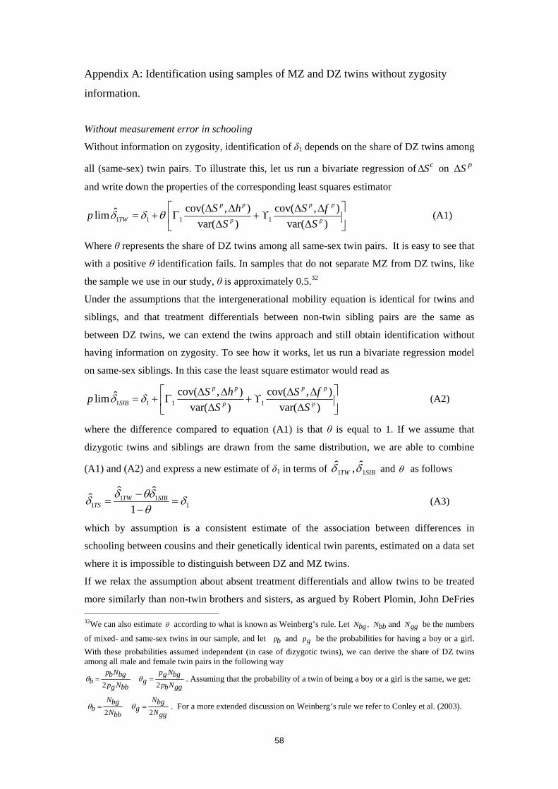
58

Appendix A: Identification using samples of MZ and DZ twins without zygosity

information.

Without measurement error in schooling

Without information on zygosity, identification of δ1 depends on the share of DZ twins among

all (same-sex) twin pairs. To illustrate this, let us run a bivariate regression of cSΔ on pSΔ

and write down the properties of the corresponding least squares estimator

1 1 1 1cov( , ) cov( , )ˆlim

var( ) var( )

p p p p

TW p p

S h S fpS S

δ δ θ⎡ ⎤Δ Δ Δ Δ

= + Γ + ϒ⎢ ⎥Δ Δ⎣ ⎦ (A1)

Where θ represents the share of DZ twins among all same-sex twin pairs. It is easy to see that

with a positive θ identification fails. In samples that do not separate MZ from DZ twins, like

the sample we use in our study, θ is approximately 0.5.32

Under the assumptions that the intergenerational mobility equation is identical for twins and

siblings, and that treatment differentials between non-twin sibling pairs are the same as

between DZ twins, we can extend the twins approach and still obtain identification without

having information on zygosity. To see how it works, let us run a bivariate regression model

on same-sex siblings. In this case the least square estimator would read as

1 1 1 1cov( , ) cov( , )ˆlim

var( ) var( )

p p p p

SIB p p

S h S fpS S

δ δ⎡ ⎤Δ Δ Δ Δ

= + Γ + ϒ⎢ ⎥Δ Δ⎣ ⎦ (A2)

where the difference compared to equation (A1) is that θ is equal to 1. If we assume that

dizygotic twins and siblings are drawn from the same distribution, we are able to combine

(A1) and (A2) and express a new estimate of δ1 in terms of SIBTW 11ˆ,ˆ δδ and θ as follows

111

1 1

ˆˆˆ δθδθδδ =

−−

= SIBTWTS (A3)

which by assumption is a consistent estimate of the association between differences in

schooling between cousins and their genetically identical twin parents, estimated on a data set

where it is impossible to distinguish between DZ and MZ twins.

If we relax the assumption about absent treatment differentials and allow twins to be treated

more similarly than non-twin brothers and sisters, as argued by Robert Plomin, John DeFries 32We can also estimate θ according to what is known as Weinberg’s rule. Let ,N Nbg bb and Ngg be the numbers

of mixed- and same-sex twins in our sample, and let pb and pg be the probabilities for having a boy or a girl. With these probabilities assumed independent (in case of dizygotic twins), we can derive the share of DZ twins among all male and female twin pairs in the following way

2 2

p N p Nb bg g bgb gp N p Ng bb b ggθ θ= = . Assuming that the probability of a twin of being a boy or a girl is the same, we get:

2 2

N Nbg bgb gN Nbb ggθ θ= = . For a more extended discussion on Weinberg’s rule we refer to Conley et al. (2003).

59

and Gerald McClearn 1990; Anders Björklund, Markus Jäntti and Gary Solon 2005, our

estimate in (B3) would underestimate the intergenerational schooling effect for the population

as whole, assuming that our sibling estimate is larger than our twin estimate TWSIB 11ˆˆ δδ > .

Although identification fails, we can still use our twins results to put meaningful lower

( TS1̂δ ) and upper bounds ( TW1̂δ ) on 1δ . Allowing for treatment differentials we have to rewrite

equation (A3) such that

1 11 1

ˆ ˆˆ1

TD TDTW SIBTS

δ λθδδ δλθ

−= =

− (A4)

If λ is smaller than 1, indicating that twins are treated more similar than non-twin siblings, it

follows that 1 1ˆ TD

TSδ δ< . So if the estimate of intergenerational effects is lower using twins

than siblings, we can bound the derived estimates in (B4) from both below and above.

With measurement error in schooling

In the case of classical measurement error in schooling, we have that for each twin parent*p pS S v= + , where pS is observed schooling, *pS is true schooling and v is a classical

measurement error (so that measurement errors are uncorrelated within families and with true

schooling). In case of classical measurement error, expression (A1) changes to

* *

1 1 1 1* *

cov( , ) cov( , )ˆlimvar( ) var( )

p p p pTW

TW Sp p

S h S fp RS S

δ δ θ Δ

⎧ ⎫⎡ ⎤Δ Δ Δ Δ⎪ ⎪= + Γ + ϒ⎨ ⎬⎢ ⎥Δ Δ⎪ ⎪⎣ ⎦⎩ ⎭ (A5)

where TWSRΔ is the reliability ratio of the twin difference in schooling, the fraction between the

variance of the true twin difference and the variance of the observed twin difference. Note the

variance and covariance terms now include true schooling instead of observed schooling.

The least squares estimator produced from the sibling fixed effects model, as depicted in (A2)

can now be expressed as

* *

1 1 1 1* *

cov( , ) cov( , )ˆlimvar( ) var( )

p p p pSIB

SIB Sp p

S h S fp RS S

δ δ Δ

⎧ ⎫⎡ ⎤Δ Δ Δ Δ⎪ ⎪= + Γ + ϒ⎨ ⎬⎢ ⎥Δ Δ⎪ ⎪⎣ ⎦⎩ ⎭ (A6)

where the differences compared to equation (A1) are that θ is equal to 1 and that the

reliability ratio in sibling-differences in schooling SIBSRΔ is allowed to be different from the

reliability ratio for twins. If we assume, as before, that dizygotic twins and siblings are drawn

from the same distribution, we are able to combine (A1) and (A2) and express a new estimate

of δ1 in terms of TW1̂δ , 1̂SIBδ , TWSRΔ , SIB

SRΔ , and θ as follows

1 11 1

ˆ ˆ ( / )1ˆ1

TW SIBTW SIB S S

TS TWS

R RR

δ θδδ δθ

Δ Δ

Δ

−= =

− (A7)

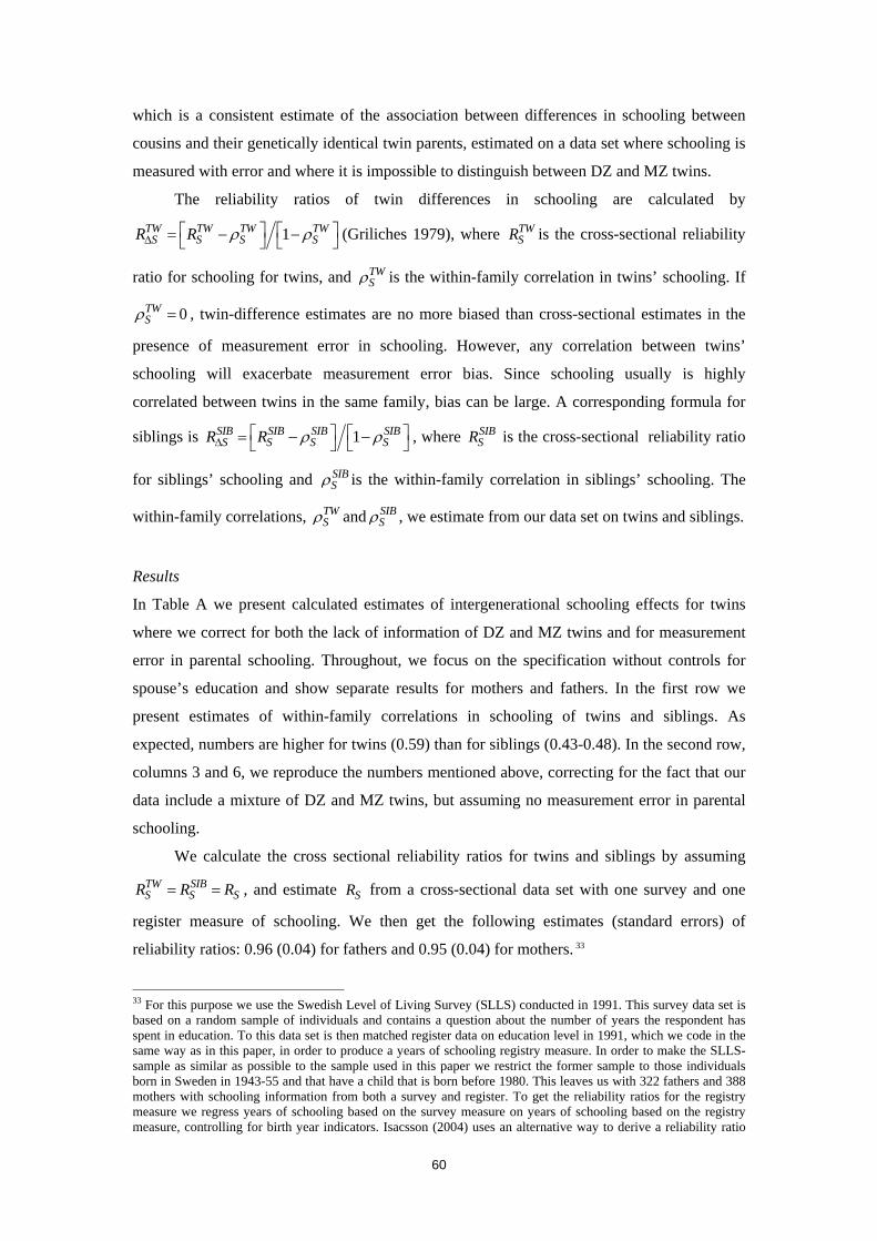
60

which is a consistent estimate of the association between differences in schooling between

cousins and their genetically identical twin parents, estimated on a data set where schooling is

measured with error and where it is impossible to distinguish between DZ and MZ twins.

The reliability ratios of twin differences in schooling are calculated by

1TW TW TW TWS S S SR R ρ ρΔ ⎡ ⎤ ⎡ ⎤= − −⎣ ⎦ ⎣ ⎦ (Griliches 1979), where TW

SR is the cross-sectional reliability

ratio for schooling for twins, and TWSρ is the within-family correlation in twins’ schooling. If

0TWSρ = , twin-difference estimates are no more biased than cross-sectional estimates in the

presence of measurement error in schooling. However, any correlation between twins’

schooling will exacerbate measurement error bias. Since schooling usually is highly

correlated between twins in the same family, bias can be large. A corresponding formula for

siblings is 1SIB SIB SIB SIBS S S SR R ρ ρΔ ⎡ ⎤ ⎡ ⎤= − −⎣ ⎦ ⎣ ⎦ , where SIB

SR is the cross-sectional reliability ratio

for siblings’ schooling and SIBSρ is the within-family correlation in siblings’ schooling. The

within-family correlations, TWSρ and SIB

Sρ , we estimate from our data set on twins and siblings.

Results

In Table A we present calculated estimates of intergenerational schooling effects for twins

where we correct for both the lack of information of DZ and MZ twins and for measurement

error in parental schooling. Throughout, we focus on the specification without controls for

spouse’s education and show separate results for mothers and fathers. In the first row we

present estimates of within-family correlations in schooling of twins and siblings. As

expected, numbers are higher for twins (0.59) than for siblings (0.43-0.48). In the second row,

columns 3 and 6, we reproduce the numbers mentioned above, correcting for the fact that our

data include a mixture of DZ and MZ twins, but assuming no measurement error in parental

schooling.

We calculate the cross sectional reliability ratios for twins and siblings by assumingTW SIBS S SR R R= = , and estimate SR from a cross-sectional data set with one survey and one

register measure of schooling. We then get the following estimates (standard errors) of

reliability ratios: 0.96 (0.04) for fathers and 0.95 (0.04) for mothers. 33

33 For this purpose we use the Swedish Level of Living Survey (SLLS) conducted in 1991. This survey data set is based on a random sample of individuals and contains a question about the number of years the respondent has spent in education. To this data set is then matched register data on education level in 1991, which we code in the same way as in this paper, in order to produce a years of schooling registry measure. In order to make the SLLS-sample as similar as possible to the sample used in this paper we restrict the former sample to those individuals born in Sweden in 1943-55 and that have a child that is born before 1980. This leaves us with 322 fathers and 388 mothers with schooling information from both a survey and register. To get the reliability ratios for the registry measure we regress years of schooling based on the survey measure on years of schooling based on the registry measure, controlling for birth year indicators. Isacsson (2004) uses an alternative way to derive a reliability ratio

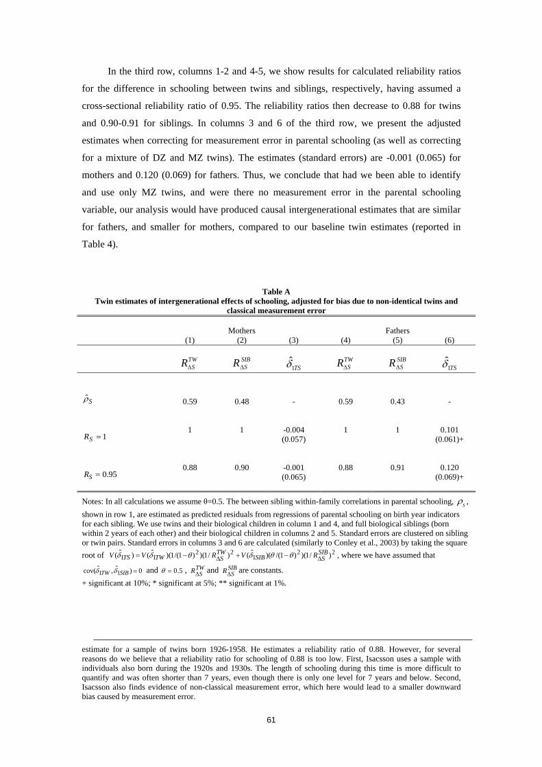
61

In the third row, columns 1-2 and 4-5, we show results for calculated reliability ratios

for the difference in schooling between twins and siblings, respectively, having assumed a

cross-sectional reliability ratio of 0.95. The reliability ratios then decrease to 0.88 for twins

and 0.90-0.91 for siblings. In columns 3 and 6 of the third row, we present the adjusted

estimates when correcting for measurement error in parental schooling (as well as correcting

for a mixture of DZ and MZ twins). The estimates (standard errors) are -0.001 (0.065) for

mothers and 0.120 (0.069) for fathers. Thus, we conclude that had we been able to identify

and use only MZ twins, and were there no measurement error in the parental schooling

variable, our analysis would have produced causal intergenerational estimates that are similar

for fathers, and smaller for mothers, compared to our baseline twin estimates (reported in

Table 4).

Table A

Twin estimates of intergenerational effects of schooling, adjusted for bias due to non-identical twins and classical measurement error

Mothers Fathers

(1) (2) (3) (4) (5) (6)

TWSRΔ SIB

SRΔ TS1̂δ TW

SRΔ SIBSRΔ TS1̂δ

Sρ̂ 0.59 0.48 - 0.59 0.43 -

1=SR 1

1

-0.004 (0.057)

1

1

0.101 (0.061)+

95.0=SR 0.88 0.90 -0.001

(0.065) 0.88 0.91 0.120

(0.069)+

Notes: In all calculations we assume θ=0.5. The between sibling within-family correlations in parental schooling, Sρ , shown in row 1, are estimated as predicted residuals from regressions of parental schooling on birth year indicators for each sibling. We use twins and their biological children in column 1 and 4, and full biological siblings (born within 2 years of each other) and their biological children in columns 2 and 5. Standard errors are clustered on sibling or twin pairs. Standard errors in columns 3 and 6 are calculated (similarly to Conley et al., 2003) by taking the square root of 22

122

11 )/1)()1/()(ˆ()/1)()1/(1)(ˆ()ˆ( SIBSSIB

TWSTWTS RVRVV ΔΔ −+−= θθδθδδ , where we have assumed that

0)ˆ,ˆcov( 11 =SIBTW δδ and 5.0=θ , TWSRΔ and SIB

SRΔ are constants. + significant at 10%; * significant at 5%; ** significant at 1%.

estimate for a sample of twins born 1926-1958. He estimates a reliability ratio of 0.88. However, for several reasons do we believe that a reliability ratio for schooling of 0.88 is too low. First, Isacsson uses a sample with individuals also born during the 1920s and 1930s. The length of schooling during this time is more difficult to quantify and was often shorter than 7 years, even though there is only one level for 7 years and below. Second, Isacsson also finds evidence of non-classical measurement error, which here would lead to a smaller downward bias caused by measurement error.

62

Appendix B: Description of the institutions of adoptions and of the compulsory

schooling reform in Sweden

The institutions of adoptions. We here briefly describe the development of Swedish and

foreign adoptions during the 1960s and 70s, and the adoption process during this time. We

draw on Frank Lindblad (2004) and Björklund, Lindahl and Plug (2004) (as well as references

therein), which we also refer to for a more thorough discussion of these issues.

Sweden is one of the countries in the world with the highest number of adopted

children per number of births. Before and up to the mid 1960s, children adopted by Swedish

parents were mostly children born in Sweden. From the mid 1960s onwards, the number of

unwanted Swedish births decreased rapidly. The reasons for this change were an increase in

social welfare, easier access to contraceptives, and less strict abortion laws. Later, it has also

become more common to place children with special needs in foster homes, instead of giving

them up for adoption. All these issues have contributed to a large decrease in the supply of

Swedish-born babies that are available for adoption. Instead, there was an increase during the

1960s in the number of foreign-born babies adopted into Swedish families. At the end of the

1960s the number of foreign-born adoptees started to reach about 1000 children per year. A

top was reached from the mid 1970s to the early 1980s when 1500-2000 foreign-born children

were adopted per year. This was almost 2 percent of all births in Sweden at that time. The

birth places of the adopted children have differed over time. At the end of the 1960s, most

children that were adopted came from Europe, whereas Asia since then has been the all

dominant supplier of babies to be adopted in Sweden. The dominating countries during the

1970s and 1980s have been South Korea, India, Sri Lanka and Colombia. In the early 20th

century, the country supplying the most adoptees is China.

During the 1960s and 1970s, the adoption process regarding Swedish-born adoptees

was organized in the following way: Couples wishing to adopt as well as (typically still

pregnant) mothers wanting to give up her child for adoption, should contact a specific social

authority responsible for the adoption process. The formal agreement by the biological mother

to give up the child for adoption should not be made until after the mother had recovered from

the delivery. Initially the child was placed in a nursery home. The social authority then started

to work on finding a suitable family among the pool of interested couples. Typically the

placement in this family was made when the child was still very young, before 6-8 months of

age. After a trial period, an application to the court about legal adoption was made.

It is clear that among the biological mothers giving up their children for adoption, those

who were younger and from lower social classes were overrepresented. With regard to the

children, adoption was not to take place if the child had a poor mental or physical health and

if those conditions were deemed hereditary. A careful investigation (including interviews) of

63

the adoptive parents was made. This was done in order to judge whether the couple was

suitable as parents and if they had good and stable economic conditions. It was also important

for adoptive parents to be tolerant, in case the child would not meet the expectations of the

parent. The parents should be at least 25 years of age and not older than that they could have

been the biological parents of the child. Newly married couples rarely featured as adoptive

parents. During the 1960s, families where the mother could stay home and take care of the

child the first couple of years were to be given priority for adoptions. In revised guidelines in

1969, affecting adoptions of Swedish babies in the 1970s, the attitude towards working

adoptive mothers appeared to have been more positive as there was no mention of such

requirements.

Matching of children to adoptive parents on some characteristics was possible since the

responsible social worker did have quite a lot of information about the biological mother (and

sometimes father). There appears, however, to have been little information available for the

adoptive parents about the biological mother, and no information travelling in the opposite

direction. The adoption guidelines for adoptions taking place in the 1960s somewhat stretched

a need for some matching (such as there not being a too large gap in talents and that physical

attributes such as height and hair colour should be similar), more than the guidelines for

adoptions in the 1970s. It also appears that adoptions made by relatives to a biological mother

were very rare during the 1960s.

A couple wishing to adopt a foreign-born baby first has to apply to a social authority in

their home municipality. They are then contacted by a social authority office, which will start

an investigation about the couple’s suitability as parents (by judging their living conditions

and their understanding of children and their needs). Based on the results in this investigation,

the social authority would make a decision of whether or not the couple was allowed to adopt.

If the answer is affirmative, the investigation is sent to an adoption agency. This agency then

presents the couple with a suggestion of a specific child, which they may or may not choose

to adopt. The parents then travel to the country of the adoptee and bring the child home. Back

in Sweden, it then may take some time for the child to be formally adopted. The latter means

that one benefit of our data is to have information on immigration date, since by this one can

more closely measure the “real” age of adoption of the child.

Description of the compulsory schooling reform.34 In the 1950s and 1960s, an educational

reform extended compulsory education in Sweden from seven (or in some cases eight) to nine

years. Prior to the reform, high-ability pupils had the option of attending the junior-secondary

school (realskola), starting either in 5th or 7th grade. Completing junior-secondary school

34 For a more thorough description of the reform, see Helena Holmlund (2007a).

64

implied a total of nine or ten years of education. Pupils who did not make it to junior-

secondary school remained throughout 7th grade in the basic comprehensive school

(folkskola), and thus completed the minimum educational requirement of seven years. The

reform introduced a new comprehensive school, which kept all pupils together in one

common school through 9th grade. The educational reform is thoroughly described in the

National Board of Education (1960) and Marklund (1980, 1981). In the following, we build

on those sources to provide a brief overview of the reform.

The reform was introduced in an effort to increase equality of opportunity, but also to

meet the increasing demand for junior-secondary school among the baby boom cohorts of the

1940s. To evaluate the appropriateness and whether the proposed nine year comprehensive

school would serve its purpose, in 1950 the Swedish parliament approved of the idea of an

experimental period at the outset of the reform. The experimental design was set up such that

gradually, some municipalities would implement the new school system, and the results

would be scrutinized before further decisions were made.

The experiment came to start in 1949/1950, and the first cohort affected was the cohort

born in 1938. The experiment, administered by the National Board of Education, was to start

throughout a whole municipality, or in certain schools within a municipality. A number of

municipalities had declared their interest in reforming their comprehensive schools. For this

reason, 264 municipalities (out of around 1,000) were asked if they were willing to introduce

the nine year school immediately or within a few years. The municipalities that were

approached had either shown interest in the reform or expanded their junior secondary school

to four years. 144 municipalities reported their interest in the reform implementation. 14

municipalities were selected for the first year of the experiment (1949/50), all of those were

required to have an eight year comprehensive school already.

The following years, the National Board of Education continued with the

implementation of the reform. Municipalities that wanted to take part in the reform were

asked to report on their population growth, on the local demand for education, tax revenues

and local school situation. For example, the availability of teachers, the number of required

teachers for the nine year comprehensive school, and the available school premises were

explored. The National Board of Education took these municipality characteristics into

account when deciding on their participation. In general, implementation of the reform started

in grades 1 and 5, the following year covering grades 1, 2, 5 and 6 and so on. From 1958 the

reform was in general introduced in grades 1-5 already from the starting year.

In 1962, the Swedish parliament came to a decision to permanently introduce the nine

year comprehensive school. At this time, the experimental period was over, and municipalities

were obliged to introduce the new compulsory school by 1969.

65

Appendix C: Estimation of pre-reform trends

We here estimate regressions of parent’s and children’s schooling on the reform (the reduced

forms), allowing the reform effect to differ for the first birth-cohort that is affected, the

cohorts that are 1, 2 and 3 years too old to have been affected and for the cohorts where the

reform already has been in effect in 1, 2, 3 or more years. Hence, we allow for reform-

dynamics both before and after the reform was implemented. If any pre-reform schooling

trends are uncorrelated with reform implementation, we expect the indicators for cohorts that

are too old to be affected to have no impact. We show estimates for parent’s schooling in

columns 1-4 and children’s schooling in columns 5-8 of Table C. The estimations always

includes cohort and municipality fixed effects, and municipality fixed effects interacted with a

linear trend in columns 2, 4, 6 and 8. In panel A, we first show reduced form estimates

assuming a constant reform effect and no impact of the reform for pre-reform cohorts. These

are the estimates underlying the IV estimates in row 2 of panel A, Table 7.

We now turn to less restrictive reduced form estimations, with resulting estimates

reported in panel B. For mothers, we find large effects of 0.12-0.17 for the cohort one year too

old to have been affected by the reform, on own schooling. These estimates are not as big as

the reform-estimates for the first cohort with reform-school, but statistically different from

zero. For mothers there is also an impact of the reform on children’s schooling for the last

cohort without the reform school. These estimates are similar to the estimates for the first

cohort with the reform in place. Hence it is clear that there is a large impact of the reform on

schooling the year prior to the introduction of the reform. This is evidence of that the key

assumption in difference-in-differences models, that treated and non-treated units experience

parallel trends, is violated for mothers. The reasons for these pre-reform effects could be

because of some measurement error in the coding of the reform, because grade repeaters are

likely to be miss-classified since we assign individuals to the reform based on their year of

birth, or due to anticipatory behaviour in part of schools in municipalities that were yet to

introduce the reform, but were expected to do so in the near future. We report p-values that

test whether the three pre-reform dummies are statistically significant from zero, and for

mothers they always are for own schooling.

These results show that the specification that controls for both municipality indicators

and municipality-specific trends probably is preferred. For fathers, there is no evidence of a

reform effect for pre-reform years. Regarding post-reform dynamics we see that, in the fixed-

effect specifications, the reform effect fades away with time. When we control for trends, the

estimates are more stable for these birth-cohorts. 35

35 Note that the reference cohorts are those passing through the education system four or more years prior to the reform. Results are very similar if we perform estimations on the extended sample of cohorts born 1934-1955. Hence, results in the table are not sensitive to the lack of pre-program periods for the early reform cohorts.

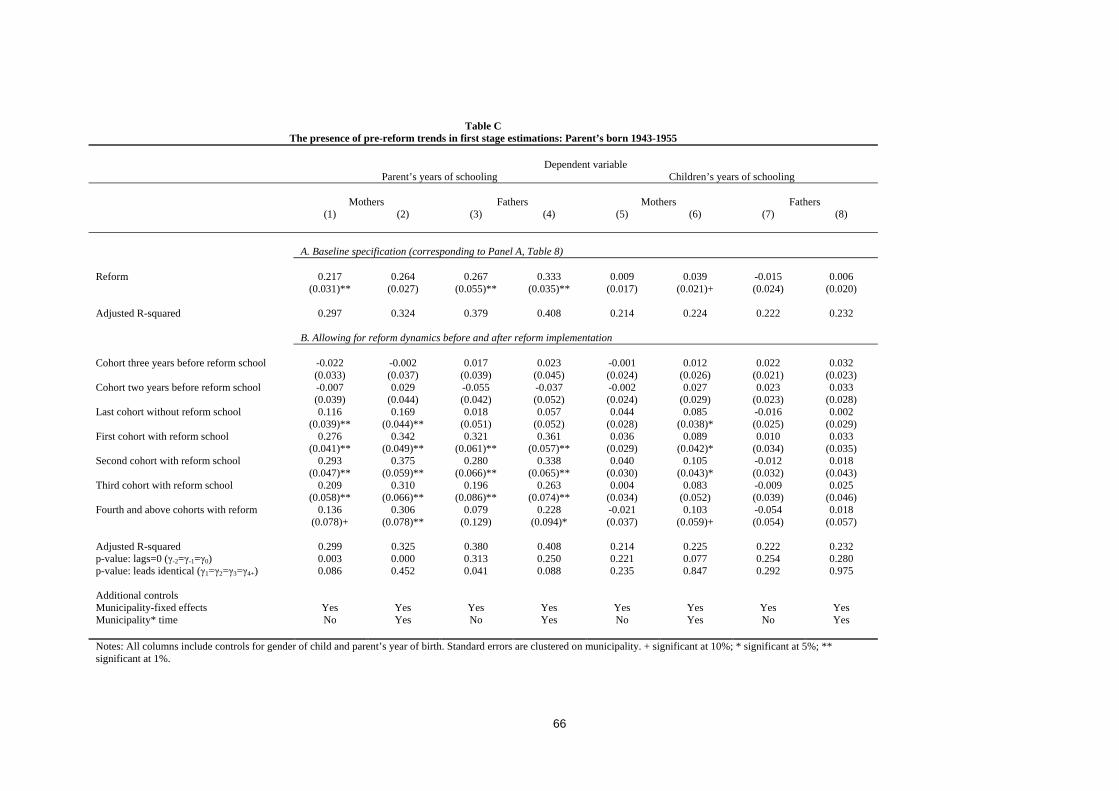
66

Table C The presence of pre-reform trends in first stage estimations: Parent’s born 1943-1955

Dependent variable Parent’s years of schooling Children’s years of schooling Mothers Fathers Mothers Fathers (1) (2) (3) (4) (5) (6) (7) (8)

A. Baseline specification (corresponding to Panel A, Table 8)

Reform

0.217 (0.031)**

0.264 (0.027)

0.267 (0.055)**

0.333 (0.035)**

0.009 (0.017)

0.039 (0.021)+

-0.015 (0.024)

0.006 (0.020)

Adjusted R-squared

0.297

0.324

0.379

0.408

0.214

0.224

0.222

0.232 B. Allowing for reform dynamics before and after reform implementation Cohort three years before reform school

-0.022 (0.033)

-0.002 (0.037)

0.017 (0.039)

0.023 (0.045)

-0.001 (0.024)

0.012 (0.026)

0.022 (0.021)

0.032 (0.023)

Cohort two years before reform school

-0.007 (0.039)

0.029 (0.044)

-0.055 (0.042)

-0.037 (0.052)

-0.002 (0.024)

0.027 (0.029)

0.023 (0.023)

0.033 (0.028)

Last cohort without reform school

0.116 (0.039)**

0.169 (0.044)**

0.018 (0.051)

0.057 (0.052)

0.044 (0.028)

0.085 (0.038)*

-0.016 (0.025)

0.002 (0.029)

First cohort with reform school

0.276 (0.041)**

0.342 (0.049)**

0.321 (0.061)**

0.361 (0.057)**

0.036 (0.029)

0.089 (0.042)*

0.010 (0.034)

0.033 (0.035)

Second cohort with reform school

0.293 (0.047)**

0.375 (0.059)**

0.280 (0.066)**

0.338 (0.065)**

0.040 (0.030)

0.105 (0.043)*

-0.012 (0.032)

0.018 (0.043)

Third cohort with reform school

0.209 (0.058)**

0.310 (0.066)**

0.196 (0.086)**

0.263 (0.074)**

0.004 (0.034)

0.083 (0.052)

-0.009 (0.039)

0.025 (0.046)

Fourth and above cohorts with reform

0.136 (0.078)+

0.306 (0.078)**

0.079 (0.129)

0.228 (0.094)*

-0.021 (0.037)

0.103 (0.059)+

-0.054 (0.054)

0.018 (0.057)

Adjusted R-squared 0.299 0.325 0.380 0.408 0.214 0.225 0.222 0.232 p-value: lags=0 (γ-2=γ-1=γ0) 0.003 0.000 0.313 0.250 0.221 0.077 0.254 0.280 p-value: leads identical (γ1=γ2=γ3=γ4+) 0.086 0.452 0.041 0.088 0.235 0.847 0.292 0.975 Additional controls Municipality-fixed effects Yes Yes Yes Yes Yes Yes Yes Yes Municipality* time No Yes No Yes No Yes No Yes Notes: All columns include controls for gender of child and parent’s year of birth. Standard errors are clustered on municipality. + significant at 10%; * significant at 5%; ** significant at 1%.

67

References Antonovics, Kate and Arthur S. Goldberger (2005), “Does Increasing Women’s Schooling Raise the Schooling of the Next Generation? Comment”, American Economic Review 95:5, pp. 1738-1744. Ashenfelter, Orley and Alan B. Krueger (1994) “Estimates of the Returns to Schooling from a New Sample of Twins”, American Economic Review 84:5, pp. 1157-1173. Ashenfelter, Orley and Cecilia Rouse, (1998), “Income, Schooling, and Ability: Evidence from a New Sample of Identical Twins", Quarterly Journal of Economics 113:1, pp. 253-284. Becker, Gary S. and Nigel Tomes (1979), “An Equilibrium Theory of the Distribution of Income and Intergenerational Mobility”, Journal of Political Economy 87:6, pp. 1153-1189. Becker, Gary S. and Nigel Tomes (1986), “Human Capital and the Rise and Fall of Families”, Journal of Labor Economics 4:3, pt 2, pp. S1-S38. Behrman, Jere R. and Mark R. Rosenzweig (2002), “Does Increasing Women’s Schooling Raise the Schooling of the Next Generation?”, American Economic Review 92:1, pp. 323-334. Behrman, Jere R. and Mark R. Rosenzweig (2004), “Returns to Birthweight”, Review of Economics and Statistics 86:2, pp. 586-601. Behrman, Jere R. and Mark R. Rosenzweig (2005), “Does Increasing Women’s Schooling Raise the Schooling of the Next Generation? Reply”, American Economic Review 95:5, pp. 1745-1751. Björklund, Anders, Markus Jäntti and Gary Solon (2005), “Influences of Nature and Nurture on Earnings Variation: A Report on a Study of Various Sibling Types in Sweden”, in Unequal Chances: Family Background and Economic Success, Samuel Bowles, Herbert Gintis and Melissa Osborne, eds. Princeton University Press. Björklund, Anders, Mikael Lindahl and Erik Plug (2004), Intergenerational effects in Sweden: What can we learn from adoption data?”, IZA discussion paper 1194.

Björklund, Anders, Mikael Lindahl and Erik Plug (2006), “The Origins of Intergenerational Associations: Lessons from Swedish Adoption Data”, Quarterly Journal of Economics 121:3, pp. 999-1028. Black, Sandra E., Paul J. Devereux and Kjell G. Salvanes (2003), “Why the Apple Doesn’t Fall Far: Understanding Intergenerational Transmission of Human Capital”, NBER working paper 10066. Black, Sandra E., Paul J. Devereux and Kjell G. Salvanes (2005), “Why the Apple Doesn’t Fall Far: Understanding Intergenerational Transmission of Human Capital”, American Economic Review 95:1, pp. 437-449. Black, Sandra E., Paul J. Devereux and Kjell G. Salvanes (2007), “From the Cradle to the Labor Market? The Effect of Birth Weight on Adult Outcomes” , Quarterly Journal of Economics 122:1, pp. 409-439. Black, Sandra E., Paul J. Devereux and Kjell G. Salvanes (2008), “Staying in the Classroom and out of the Maternity Ward? The Effect of Compulsory Schooling Laws on Teenage Births”, Economic Journal 118:530, pp. 1025-1054.

68

Bohman, Michael (1970), Adopted Children and their Families, Stockholm: Proprius. Bonjour, Dorothe, Lynn Cherkas, Jonathan Haskel, Denise Hawkes and Tim Spector (2003), “Returns to Education: Evidence from UK Twins”, American Economic Review 93:5, pp. 1799-1812. Bound, John and Gary Solon (1999), “Double Trouble: On the Value of Twins-Based Estimation of the Return to Schooling”, Economics of Education Review 18:2, pp. 169-182. Carneiro, Pedro, Costats Meghir and Matthias Parey (2007), “Maternal Education, Home Environments and the Development of Children and Adolescents”, IZA discussion paper No. 3072. Chevalier, Arnaud (2004), “Parental Education and Child’s Education: A Natural Experiment”, IZA discussion paper No. 1153. Conley, Dalton, Kate Strully and Neil G. Bennett (2003), “A Pound of Flesh or Just Proxy? Using Twin Differences to Estimate the Effect of Birth Weight on Life Chances”, NBER WP 9901. Dearden, Lorraine S., Stephen Machin and Howard Reed (1997), “Intergenerational Mobility in Britain”, Economic Journal 110:440, pp. 47-64. De Haan, Monique and Erik Plug (2006), “Estimates of the Effects of Parents’ Schooling on Children’s Schooling Using Censored and Uncensored Samples”, IZA discussion paper No. 2416. Grawe, Nathan and Casey Mulligan (2002), “Economic Interpretations of Intergenerational Correlations”, Journal of Economic Perspectives 16:3, pp. 45-58. Griliches, Zvi (1979), “Sibling Models and Data in Economics: Beginnings of a Survey”, Journal of Political Economy 87:5, pp. 37-64. Haveman, Robert and Barbara Wolfe (1995), “The Determinants of Children Attainments: A Review of Methods and Findings”, Journal of Economic Literature 33:4, pp. 1829-1878. Heston, Alan, Robert Summers and Bettina Aten (2002), Penn World Table Version 6.1, Center for International Comparisons at the University of Pennsylvania (CICUP). Holmlund, Helena (2007a), “A Researcher’s Guide to the Swedish Compulsory Schooling reform”, working paper 9/2007, Swedish Institute for Social Research. Holmlund, Helena (2007b), “Intergenerational Mobility and Assortative Mating: Effects of An Educational Reform”, revised version of working paper 4/2006, Swedish Institute for Social Research. Isacsson, Gunnar (1999), “Estimates of the Return to Schooling in Sweden from a Large Sample of Twins”, Labour Economics 6:4, pp. 471-489 Isacsson, Gunnar (2004), “Estimating the Economic Return to Educational Levels Using Data on Twins”, Journal of Applied Econometrics 19:1, pp. 99-119. Lindblad, Frank (2004), Adoption, Lund, Studentlitteratur. Kim, Wun-Jung (1995), ”International adoption: A case review of Korean children”, Child Psychiatry and Human Development 25:3, Spring, pp. 141-154 Maurin, Eric and Sandra McNally (2008), “Vive la Révolution! Long Term Returns of 1968 to the Angry Students”, Journal of Labour Economics 26:1, pp. 1-33.

69

Marklund, Sixten (1980), Från Reform till Reform: Skolsverige 1950-1975, Del 1, 1950 års Reformbeslut. Skolöverstyrelsen och Liber UtbildninsFörlaget. Marklund, Sixten (1981), Från Reform till Reform: Skolsverige 1950-1975, Del 2, Försöksverksamheten. Skolöverstyrelsen och Liber UtbildninsFörlaget. Meghir, Costas and Mårten Palme (2003), “Ability, Parental Background and Educational Policy: Empirical Evidence from a Social Experiment”, Institute of Fiscal Studies, IFS working paper W03/05. Meghir, Costas and Mårten Palme (2005), “Educational Reform, Ability, and Family Background”, American Economic Review 95:1, pp. 414-424. National Board of Education (Skolöverstyrelsen) (1954-1962), ”Redogörelse för försöksverksamhet med enhetsskola”, Aktuellt från Skolöverstyrelsen. Oreopoulos, Philip, Marianne Page and Anne Huff Stevens (2003), “Does Human Capital Transfer from Parent to Child? The Intergenerational Effects of Compulsory Schooling”, NBER working paper 10164. Oreopoulos, Philip, Marianne Page and Anne Huff Stevens (2006), “The Intergenerational Effects of Compulsory Schooling”, Journal of Labor Economics 24:4, pp. 729-760. Plomin, Robert, John C. DeFries and Gerald E. McClearn (1990), Behavioral Genetics: A Primer. 3d ed. New York: W.H. Freeman, 1990. Plug, Erik (2004) “Estimating the Effect of Mother’s Schooling on Children’s Schooling Using a Sample of Adoptees”, American Economic Review 94:1, pp. 358-368. Plug, Erik and Wim Vijverberg (2003), “Schooling, Family Background, and Adoption: Is it Nature or Is it Nurture?”, Journal of Political Economics 111:3, pp. 611-641. Sacerdote, Bruce (2000), “The Nature and Nurture of Economic Outcomes”, NBER working paper 7949. Sacerdote, Bruce (2002), “The Nature and Nurture of Economic Outcomes”, American Economic Review (Papers and Proceedings) 92:2, pp. 344-348. Sacerdote, Bruce (2007), “What Happens When We Randomly Assign Children to Families”, Quarterly Journal of Economics, forthcoming. Schultz, T. Paul (2002), “Why Governments Should Invest More to Educate Girls”, Journal of World Development 30:2, pp. 207-225. Solon, Gary (1999), “Intergenerational Mobility in the Labor Market”, in Handbook of Labor Economics. Vol. III. Orley Ashenfelter and David Card, eds. Amsterdam: North-Holland, pp. 1761-1800. Solon, Gary (2004), “A Model of Intergenerational Mobility Variation over Time and Place”, in Generational Income Mobility in North America and Europe, Miles Corak ed., Cambridge University Press. Wolfers, Justin (2006), “Did Unilateral Divorce Raise Divorce Rates? A Reconciliation and New Results”, American Economic Review 96(5), pp. 1802-1820.

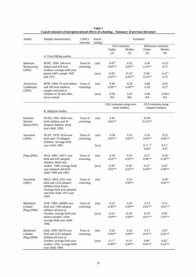
70

Table 1 Causal estimates of intergenerational effects of schooling – Summary of previous literature

Author Sample characteristics Child’s

outcome Assort. mating

Estimates

OLS estimates Difference estimates Father

(1) Mother

(2) Father

(3) Mother

(4) A. Twin/Sibling studies Behrman Rosenzweig (2002)

MTRa, 1994: 244 twin fathers and 424 twin mothers; average birth year parent 1947; sample 1947 and 1971.

Years of schooling

(no)

(yes)

0.47b

0.05**

0.33c

0.07**

0.33 0.05**

0.14 c

0.05**

0.36 0.16**

0.34 c

0.16**

-0.25 0.15

-0.27 c 0.15

Antonovics Goldberger (2005)

MTR, 1994: 92 twin fathers and 180 twin mothers; sample restricted to children of 18 and older, not in school.

Years of schooling

(no)

(yes)

0.49 0.09**

0.50 NA

0.28 0.09**

0.10 NA

0.48 0.16

0.48 NA

0.03 0.27

-0.003

NA

B. Adoption studies

OLS estimates using own-birth children

OLS estimates using adopted children

Dearden Machin Reed (1997)

NCDS, 1991: 4030 own birth children and 41 adopted children. Birth year child: 1958.

Years of schooling

(no) 0.42 0.02**

0.356 0.123**

Sacerdote (2000)

NLSY, 1979: 5614 own birth and 170 adopted children. Average birth year child: 1961.

Years of schooling

(no)

(yes)

0.28 0.01**

0.35 0.01**

0.16 0.04**

0.11 c,d 0.04*

0.22 0.06**

0.11 c 0.07

Plug (2004) WLS, 1992: 15871 own

birth and 610 adopted children. Birth year mother: 1940, average birth year adopted and birth child: 1969 and 1965.

Years of schooling

(no)

(yes)

0.39 0.01**

0.30 c

0.01**

0.54 0.02**

0.30 c

0.02**

0.27 0.04**

0.23 c

0.04**

0.28 0.10**

0.10 c

0.08**

Sacerdote (2007)

HICS, 2003: 1051 own birth and 1256 adopted children from Korea. Average birth year adopted and birth child: 1975 and 1969.

Years of schooling

(no)

0.32 0.04**

0.09 0.03**

Björklund Lindahl Plug (2004)

SAR, 1999: 148496 own birth and 7498 adopted children all born in Sweden; average birth year adotive mother; 1934; average birth year child: 1966.

Years of schooling

(no)

(yes)

0.23 0.00**

0.16 c

0.00**

0.24 0.00**

0.16 c

0.00**

0.13 0.01**

0.10c

0.01**

0.11 0.01**

0.06 c

0.01**

Björklund Lindahl Plug (2006)

SAR, 1999: 94079 own birth and 2125 adopted children all born in Sweden; average birth year mother: 1932; average birth year child: 1964.

Years of schooling

(no)

(yes)

0.24 0.00**

0.17 c

0.00**

0.24 0.00**

0.16 c

0.00**

0.11 0.01**

0.09 c

0.01**

0.07 0.01**

0.02 c

0.01**

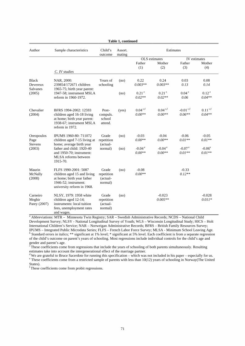
71

Table 1, continued

Author Sample characteristics Child’s

outcome Assort. mating

Estimates

OLS estimates IV estimates Father

(1) Mother

(2) Father

(3) Mother

(4) C. IV studies Black Devereux Salvanes (2005)

NAR, 2000: 239854/172671 children 1965-75; birth year parent: 1947-58; instrument MSLA reform in 1960-1972.

Years of schooling

(no)

(no)

0.22 0.003**

0.21 e

0.02**

0.24 0.003**

0.21 e

0.02**

0.03 0.13

0.04 e 0.06

0.08 0.14

0.12 e

0.04**

Chevalier (2004)

BFRS 1994-2002: 12593 children aged 16-18 living at home; birth year parent: 1938-67; instrument MSLA reform in 1972.

Post-compuls.

school attend.

(yes) 0.04 c,f 0.00**

0.04 c,f 0.00**

-0.01 c,f 0.06**

0.11 c,f 0.04**

Oreopoulos Page Stevens (2003)

IPUMS 1960-80: 711072 children aged 7-15 living at home; average birth year father and child: 1920-40 and 1950-70; instrument: MLSA reforms between 1915-70.

Grade repetition (actual-normal)

(no)

(no)

-0.03 0.00**

-0.04 e 0.00**

-0.04 0.00**

-0.04 e 0.00**

-0.06 0.01**

-0.07 e 0.01**

-0.05 0.01**

-0.06e 0.01**

Maurin McNally (2008)

FLFS 1990-2001: 5087 children aged 15 and living at home; birth year father 1946-52; instrument: university reform in 1968.

Grade repetition (actual-normal)

(no) -0.08 0.00**

-0.33 0.12**

Carneiro Meghir Parey (2007)

NLSY, 1979: 1958 white children aged 12-14; instruments: local tuition fees, unemployment rates and wages.

Grade repetition (actual-normal)

(no) -0.023 0.005**

-0.028 0.011*

a Abbreviations: MTR – Minnesota Twin Registry; SAR – Swedish Administrative Records; NCDS – National Child Development Survey; NLSY - National Longitudinal Survey of Youth; WLS – Wisconsin Longitudinal Study; HICS – Holt International Children’s Service; NAR – Norweigan Administrative Records; BFRS – British Family Resources Survey; IPUMS – Integrated Public Microdata Series; FLFS – French Labor Force Survey; MLSA - Minimum School Leaving Age. b Standard errors in italics; ** significant at 1% level; * significant at 5% level. Each coefficient is from a separate regression of the child’s outcome on parent’s years of schooling. Most regressions include individual controls for the child’s age and gender and parent’s age. c These coefficients come from regressions that include the years of schooling of both parents simultaneously. Resulting estimates take into account the intergenerational effect of the marriage partner. d We are grateful to Bruce Sacerdote for running this specification – which was not included in his paper – especially for us. e These coefficients come from a restricted sample of parents with less than 10(12) years of schooling in Norway(The United States). f These coefficients come from probit regressions.

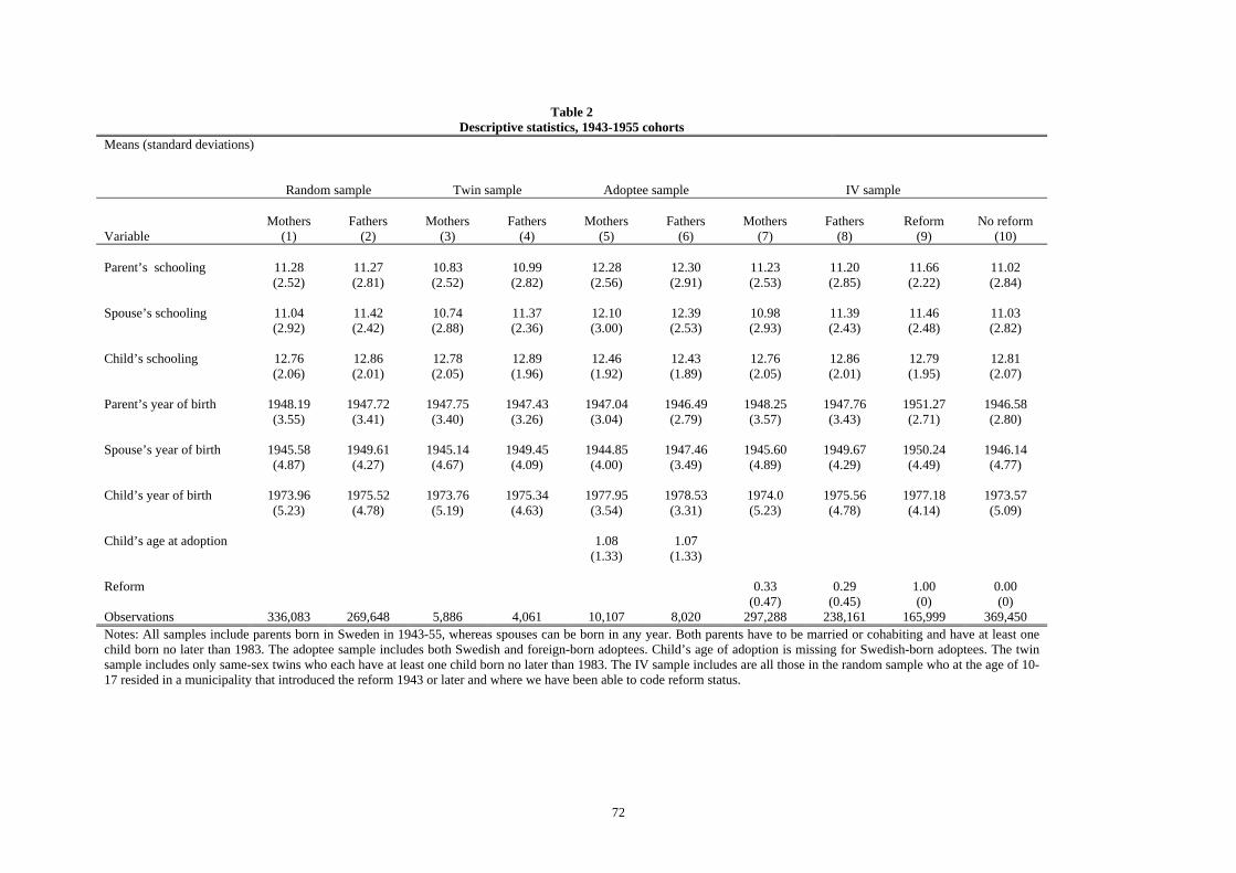
72

Table 2 Descriptive statistics, 1943-1955 cohorts

Means (standard deviations)

Random sample

Twin sample

Adoptee sample

IV sample

Mothers Fathers Mothers Fathers Mothers Fathers Mothers Fathers Reform No reform Variable (1) (2) (3) (4) (5) (6) (7) (8) (9) (10) Parent’s schooling 11.28 11.27 10.83 10.99 12.28 12.30 11.23 11.20 11.66 11.02 (2.52) (2.81) (2.52) (2.82) (2.56) (2.91) (2.53) (2.85) (2.22) (2.84) Spouse’s schooling 11.04 11.42 10.74 11.37 12.10 12.39 10.98 11.39 11.46 11.03 (2.92) (2.42) (2.88) (2.36) (3.00) (2.53) (2.93) (2.43) (2.48) (2.82) Child’s schooling 12.76 12.86 12.78 12.89 12.46 12.43 12.76 12.86 12.79 12.81 (2.06) (2.01) (2.05) (1.96) (1.92) (1.89) (2.05) (2.01) (1.95) (2.07) Parent’s year of birth 1948.19 1947.72 1947.75 1947.43 1947.04 1946.49 1948.25 1947.76 1951.27 1946.58 (3.55) (3.41) (3.40) (3.26) (3.04) (2.79) (3.57) (3.43) (2.71) (2.80) Spouse’s year of birth 1945.58 1949.61 1945.14 1949.45 1944.85 1947.46 1945.60 1949.67 1950.24 1946.14 (4.87) (4.27) (4.67) (4.09) (4.00) (3.49) (4.89) (4.29) (4.49) (4.77) Child’s year of birth 1973.96 1975.52 1973.76 1975.34 1977.95 1978.53 1974.0 1975.56 1977.18 1973.57 (5.23) (4.78) (5.19) (4.63) (3.54) (3.31) (5.23) (4.78) (4.14) (5.09) Child’s age at adoption 1.08 1.07 (1.33) (1.33) Reform 0.33 0.29 1.00 0.00 (0.47) (0.45) (0) (0) Observations 336,083 269,648 5,886 4,061 10,107 8,020 297,288 238,161 165,999 369,450 Notes: All samples include parents born in Sweden in 1943-55, whereas spouses can be born in any year. Both parents have to be married or cohabiting and have at least one child born no later than 1983. The adoptee sample includes both Swedish and foreign-born adoptees. Child’s age of adoption is missing for Swedish-born adoptees. The twin sample includes only same-sex twins who each have at least one child born no later than 1983. The IV sample includes are all those in the random sample who at the age of 10-17 resided in a municipality that introduced the reform 1943 or later and where we have been able to code reform status.

73

Table 3

OLS estimates of intergenerational effects of schooling on the random sample Dependent variable: Child’s years of schooling

Mothers Fathers (1) (2) A. Baseline specification Parent’s schooling 0.282 0.233 (0.002)** (0.001)** R-squared 0.13 0.12 B. Controlling for education of the spouse Parent’s schooling 0.198 0.152 (0.002)** (0.002)** R-squared 0.17 0.17 C. Non-linear effects of schooling Parent’s schooling -0.041 -0.077 (0.012)** (0.011)** Parent’s schooling squared 0.014 0.014 (0.001)** (0.000)** R-squared 0.14 0.13 Observations 336,083 269,648

Notes: Estimates on a 35 percent random sample of cohorts born in Sweden in 1943-1955. Controls: gender of child, parent’s year of birth. The second panel also controls for spouse’s years of schooling and year of birth. Standard errors are clustered on family.+ significant at 10%; * significant at 5%; ** significant at 1%.

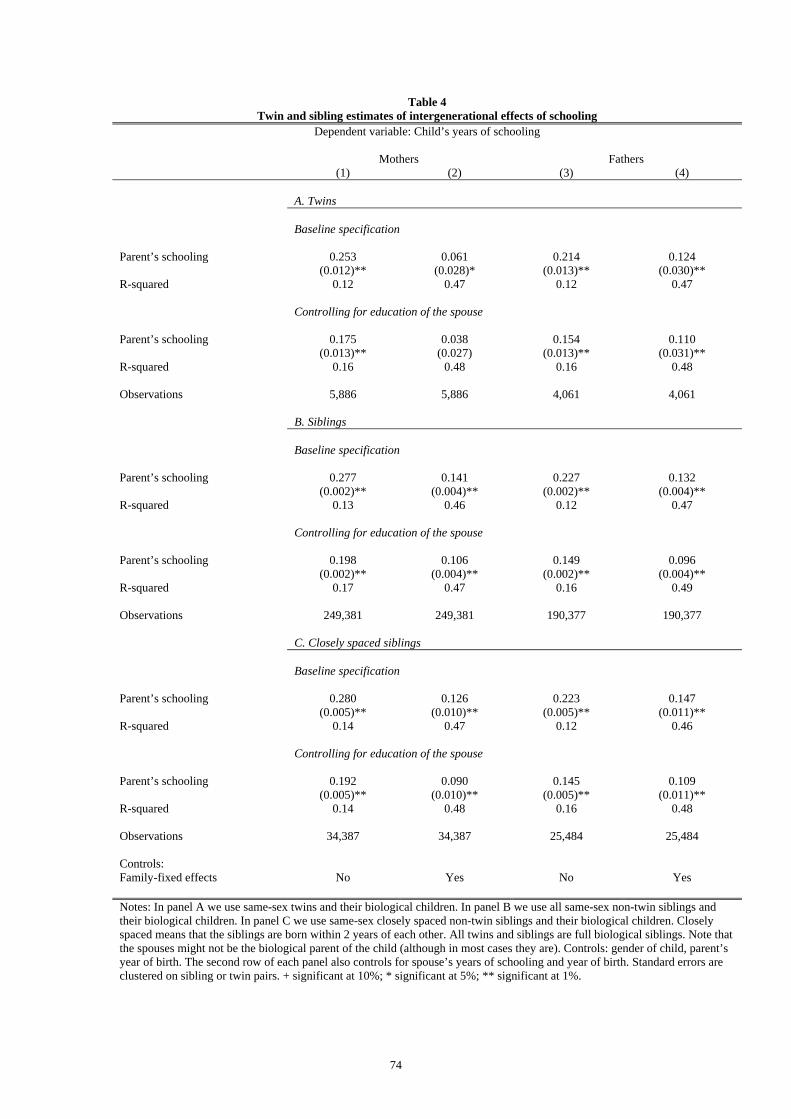
74

Table 4 Twin and sibling estimates of intergenerational effects of schooling

Dependent variable: Child’s years of schooling Mothers Fathers (1) (2) (3) (4) A. Twins Baseline specification

Parent’s schooling

0.253 (0.012)**

0.061 (0.028)*

0.214 (0.013)**

0.124 (0.030)**

R-squared 0.12 0.47 0.12 0.47

Controlling for education of the spouse

Parent’s schooling

0.175 (0.013)**

0.038 (0.027)

0.154 (0.013)**

0.110 (0.031)**

R-squared 0.16 0.48 0.16 0.48 Observations 5,886 5,886 4,061 4,061 B. Siblings Baseline specification

Parent’s schooling

0.277 (0.002)**

0.141 (0.004)**

0.227 (0.002)**

0.132 (0.004)**

R-squared 0.13 0.46 0.12 0.47

Controlling for education of the spouse

Parent’s schooling

0.198 (0.002)**

0.106 (0.004)**

0.149 (0.002)**

0.096 (0.004)**

R-squared 0.17 0.47 0.16 0.49 Observations 249,381 249,381 190,377 190,377 C. Closely spaced siblings Baseline specification

Parent’s schooling

0.280 (0.005)**

0.126 (0.010)**

0.223 (0.005)**

0.147 (0.011)**

R-squared 0.14 0.47 0.12 0.46

Controlling for education of the spouse

Parent’s schooling

0.192 (0.005)**

0.090 (0.010)**

0.145 (0.005)**

0.109 (0.011)**

R-squared 0.14 0.48 0.16 0.48 Observations 34,387 34,387 25,484 25,484 Controls: Family-fixed effects No Yes No Yes Notes: In panel A we use same-sex twins and their biological children. In panel B we use all same-sex non-twin siblings and their biological children. In panel C we use same-sex closely spaced non-twin siblings and their biological children. Closely spaced means that the siblings are born within 2 years of each other. All twins and siblings are full biological siblings. Note that the spouses might not be the biological parent of the child (although in most cases they are). Controls: gender of child, parent’s year of birth. The second row of each panel also controls for spouse’s years of schooling and year of birth. Standard errors are clustered on sibling or twin pairs. + significant at 10%; * significant at 5%; ** significant at 1%.

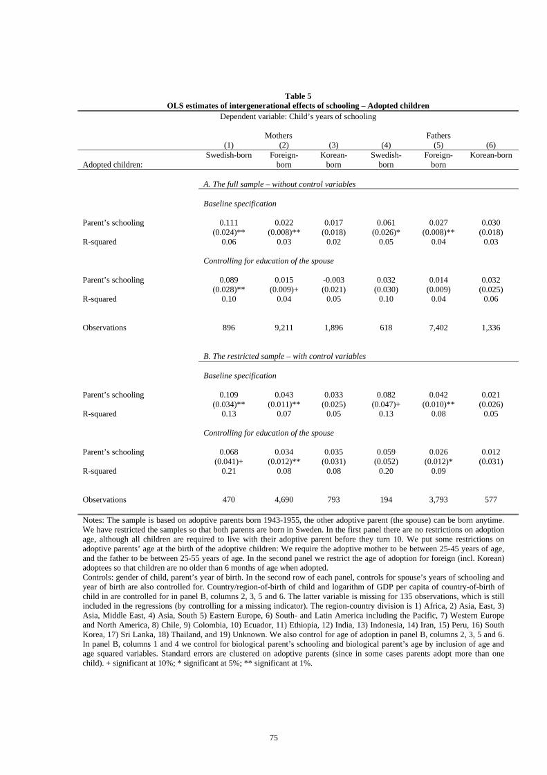
75

Table 5 OLS estimates of intergenerational effects of schooling – Adopted children

Dependent variable: Child’s years of schooling Mothers Fathers (1) (2) (3) (4) (5) (6)

Adopted children: Swedish-born Foreign-

born Korean-

born Swedish-

born Foreign-

born Korean-born

A. The full sample – without control variables

Baseline specification

Parent’s schooling

0.111 (0.024)**

0.022 (0.008)**

0.017 (0.018)

0.061 (0.026)*

0.027 (0.008)**

0.030 (0.018)

R-squared 0.06 0.03 0.02 0.05 0.04 0.03

Controlling for education of the spouse

Parent’s schooling

0.089 (0.028)**

0.015 (0.009)+

-0.003 (0.021)

0.032 (0.030)

0.014 (0.009)

0.032 (0.025)

R-squared 0.10 0.04 0.05 0.10 0.04 0.06 Observations 896 9,211 1,896 618 7,402 1,336 B. The restricted sample – with control variables

Baseline specification

Parent’s schooling

0.109 (0.034)**

0.043 (0.011)**

0.033 (0.025)

0.082 (0.047)+

0.042 (0.010)**

0.021 (0.026)

R-squared 0.13 0.07 0.05 0.13 0.08 0.05

Controlling for education of the spouse

Parent’s schooling

0.068 (0.041)+

0.034 (0.012)**

0.035 (0.031)

0.059 (0.052)

0.026 (0.012)*

0.012 (0.031)

R-squared 0.21 0.08 0.08 0.20 0.09 Observations 470 4,690 793 194 3,793 577 Notes: The sample is based on adoptive parents born 1943-1955, the other adoptive parent (the spouse) can be born anytime. We have restricted the samples so that both parents are born in Sweden. In the first panel there are no restrictions on adoption age, although all children are required to live with their adoptive parent before they turn 10. We put some restrictions on adoptive parents’ age at the birth of the adoptive children: We require the adoptive mother to be between 25-45 years of age, and the father to be between 25-55 years of age. In the second panel we restrict the age of adoption for foreign (incl. Korean) adoptees so that children are no older than 6 months of age when adopted. Controls: gender of child, parent’s year of birth. In the second row of each panel, controls for spouse’s years of schooling and year of birth are also controlled for. Country/region-of-birth of child and logarithm of GDP per capita of country-of-birth of child in are controlled for in panel B, columns 2, 3, 5 and 6. The latter variable is missing for 135 observations, which is still included in the regressions (by controlling for a missing indicator). The region-country division is 1) Africa, 2) Asia, East, 3) Asia, Middle East, 4) Asia, South 5) Eastern Europe, 6) South- and Latin America including the Pacific, 7) Western Europe and North America, 8) Chile, 9) Colombia, 10) Ecuador, 11) Ethiopia, 12) India, 13) Indonesia, 14) Iran, 15) Peru, 16) South Korea, 17) Sri Lanka, 18) Thailand, and 19) Unknown. We also control for age of adoption in panel B, columns 2, 3, 5 and 6. In panel B, columns 1 and 4 we control for biological parent’s schooling and biological parent’s age by inclusion of age and age squared variables. Standard errors are clustered on adoptive parents (since in some cases parents adopt more than one child). + significant at 10%; * significant at 5%; ** significant at 1%.

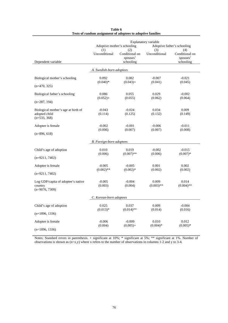
76

Table 6 Tests of random assignment of adoptees to adoptive families

Explanatory variable Adoptive mother’s schooling Adoptive father’s schooling

Dependent variable

(1) Unconditional

(2) Conditional on

spouses’ schooling

(3) Unconditional

(4) Conditional on

spouses’ schooling

A. Swedish-born adoptees Biological mother’s schooling

0.092 (0.040)*

0.082 (0.043)+

-0.007 (0.041)

-0.021 (0.045)

(n=470, 325) Biological father’s schooling

0.086 (0.052)+

0.055 (0.055)

0.029 (0.062)

-0.002 (0.064)

(n=287, 194) Biological mother’s age at birth of adopted child

-0.043 (0.114)

-0.024 (0.125)

0.034 (0.132)

0.009 (0.149)

(n=533, 368) Adoptee is female

-0.002 (0.006)

-0.001 (0.007)

-0.006 (0.007)

-0.011 (0.008)

(n=896, 618) B. Foreign-born adoptees Child’s age of adoption

0.010 (0.006)

0.019 (0.007)**

-0.002 (0.006)

-0.015 (0.007)*

(n=9211, 7402) Adoptee is female

-0.005 (0.002)**

-0.005 (0.002)*

0.001 (0.002)

0.002 (0.002)

(n=9211, 7402) Log GDP/capita of adoptee’s native country

-0.005 (0.003)

-0.004 (0.004)

0.009 (0.003)**

0.014 (0.004)**

(n=9076, 7309) C. Korean-born adoptees Child’s age of adoption

0.025 (0.013)*

0.037 (0.014)**

0.009 (0.014)

-0.004 (0.016)

(n=1896, 1336) Adoptee is female

-0.006 (0.004)

-0.009 (0.005)+

0.010 (0.004)*

0.012 (0.005)*

(n=1896, 1336) Notes: Standard errors in parenthesis. + significant at 10%; * significant at 5%; ** significant at 1%. Number of observations is shown as (n=x,y) where x refers to the number of observations in columns 1-2 and y to 3-4.

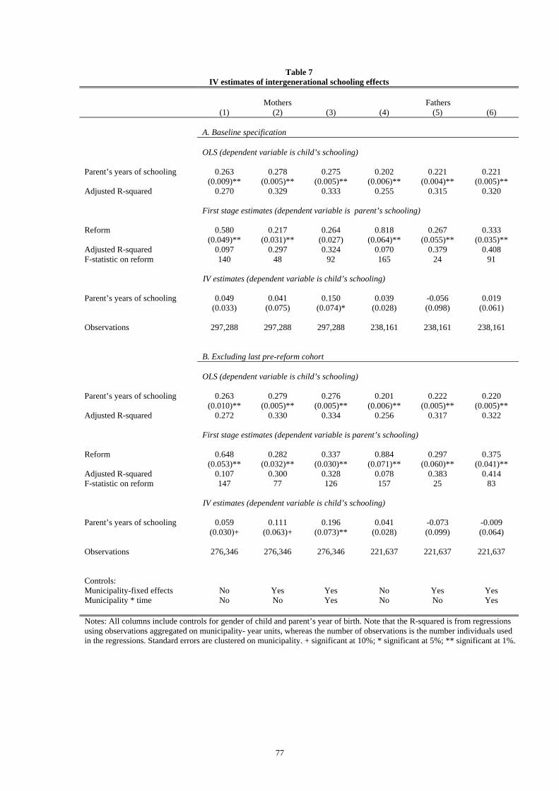
77

Table 7 IV estimates of intergenerational schooling effects

Mothers Fathers

(1) (2) (3) (4) (5) (6) A. Baseline specification OLS (dependent variable is child’s schooling)

Parent’s years of schooling 0.263

(0.009)** 0.278

(0.005)** 0.275

(0.005)** 0.202

(0.006)** 0.221

(0.004)** 0.221

(0.005)** Adjusted R-squared 0.270 0.329 0.333 0.255 0.315 0.320

First stage estimates (dependent variable is parent’s schooling)

Reform

0.580 (0.049)**

0.217 (0.031)**

0.264 (0.027)

0.818 (0.064)**

0.267 (0.055)**

0.333 (0.035)**

Adjusted R-squared 0.097 0.297 0.324 0.070 0.379 0.408 F-statistic on reform 140 48 92 165 24 91

IV estimates (dependent variable is child’s schooling)

Parent’s years of schooling

0.049 (0.033)

0.041 (0.075)

0.150 (0.074)*

0.039 (0.028)

-0.056 (0.098)

0.019 (0.061)

Observations 297,288 297,288 297,288 238,161 238,161 238,161 B. Excluding last pre-reform cohort OLS (dependent variable is child’s schooling)

Parent’s years of schooling

0.263 (0.010)**

0.279 (0.005)**

0.276 (0.005)**

0.201 (0.006)**

0.222 (0.005)**

0.220 (0.005)**

Adjusted R-squared 0.272 0.330 0.334 0.256 0.317 0.322

First stage estimates (dependent variable is parent’s schooling)

Reform

0.648 (0.053)**

0.282 (0.032)**

0.337 (0.030)**

0.884 (0.071)**

0.297 (0.060)**

0.375 (0.041)**

Adjusted R-squared 0.107 0.300 0.328 0.078 0.383 0.414 F-statistic on reform 147 77 126 157 25 83

IV estimates (dependent variable is child’s schooling)

Parent’s years of schooling

0.059 (0.030)+

0.111 (0.063)+

0.196 (0.073)**

0.041 (0.028)

-0.073 (0.099)

-0.009 (0.064)

Observations 276,346 276,346 276,346 221,637 221,637 221,637 Controls: Municipality-fixed effects No Yes Yes No Yes Yes Municipality * time No No Yes No No Yes Notes: All columns include controls for gender of child and parent’s year of birth. Note that the R-squared is from regressions using observations aggregated on municipality- year units, whereas the number of observations is the number individuals used in the regressions. Standard errors are clustered on municipality. + significant at 10%; * significant at 5%; ** significant at 1%.

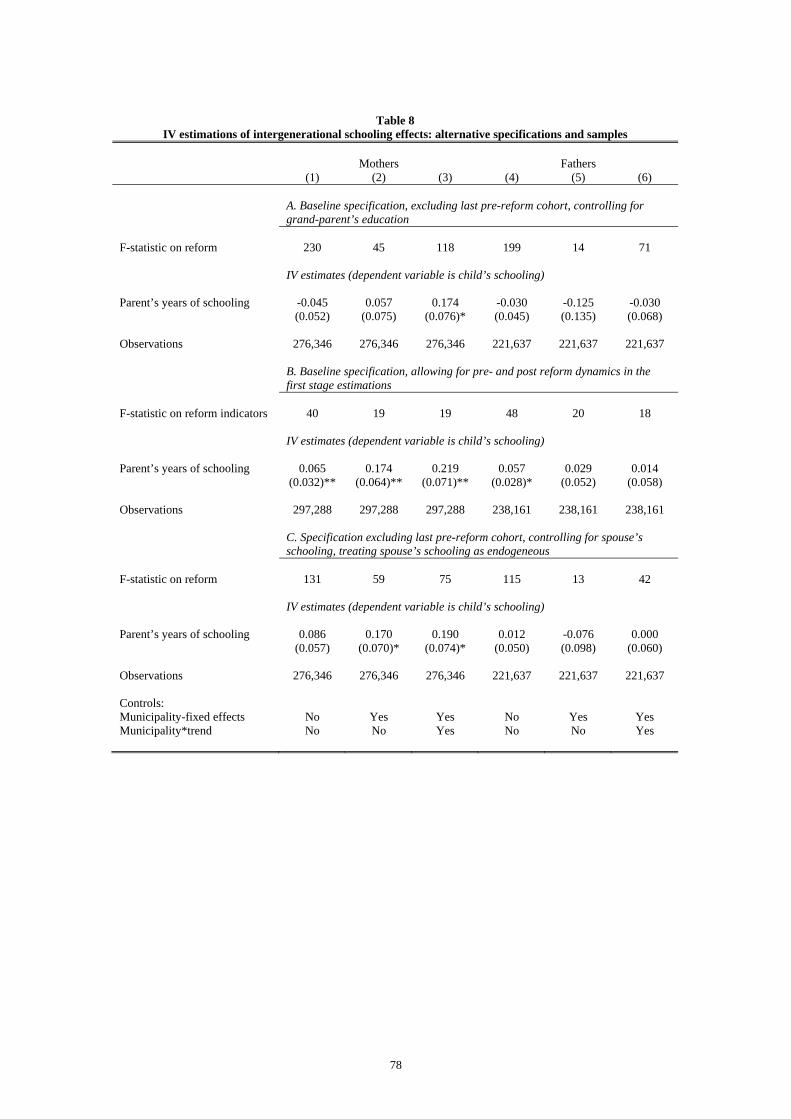
78

Table 8

IV estimations of intergenerational schooling effects: alternative specifications and samples Mothers Fathers (1) (2) (3) (4) (5) (6)

A. Baseline specification, excluding last pre-reform cohort, controlling for grand-parent’s education

F-statistic on reform 230 45 118 199 14 71

IV estimates (dependent variable is child’s schooling)

Parent’s years of schooling

-0.045 (0.052)

0.057 (0.075)

0.174 (0.076)*

-0.030 (0.045)

-0.125 (0.135)

-0.030 (0.068)

Observations 276,346 276,346 276,346 221,637 221,637 221,637

B. Baseline specification, allowing for pre- and post reform dynamics in the first stage estimations

F-statistic on reform indicators 40 19 19 48 20 18

IV estimates (dependent variable is child’s schooling)

Parent’s years of schooling

0.065 (0.032)**

0.174 (0.064)**

0.219 (0.071)**

0.057 (0.028)*

0.029 (0.052)

0.014 (0.058)

Observations 297,288 297,288 297,288 238,161 238,161 238,161

C. Specification excluding last pre-reform cohort, controlling for spouse’s schooling, treating spouse’s schooling as endogeneous

F-statistic on reform 131 59 75 115 13 42

IV estimates (dependent variable is child’s schooling)

Parent’s years of schooling

0.086 (0.057)

0.170 (0.070)*

0.190 (0.074)*

0.012 (0.050)

-0.076 (0.098)

0.000 (0.060)

Observations 276,346 276,346 276,346 221,637 221,637 221,637 Controls: Municipality-fixed effects No Yes Yes No Yes Yes Municipality*trend No No Yes No No Yes

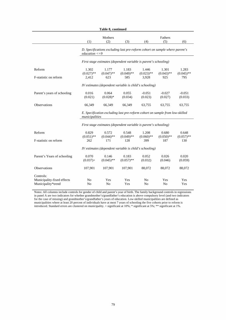
79

Table 8, continued Mothers Fathers (1) (2) (3) (4) (5) (6)

D. Specifications excluding last pre-reform cohort on sample where parent’s education <=9

First stage estimates (dependent variable is parent’s schooling)

Reform

1.302 (0.027)**

1.177 (0.047)**

1.183 (0.049)**

1.446 (0.023)**

1.301 (0.043)**

1.283 (0.045)**

F-statistic on reform 2,412 623 585 3,928 925 795

IV estimates (dependent variable is child’s schooling)

Parent’s years of schooling

0.016 (0.021)

0.064 (0.028)*

0.055 (0.034)

-0.051 (0.023)

-0.027 (0.027)

-0.051 (0.033)

Observations 66,349 66,349 66,349 63,755 63,755 63,755

E. Specification excluding last pre-reform cohort on sample from low-skilled municipalities

First stage estimates (dependent variable is parent’s schooling)

Reform

0.829 (0.051)**

0.572 (0.044)**

0.548 (0.049)**

1.208 (0.060)**

0.680 (0.050)**

0.648 (0.057)**

F-statistic on reform 262 171 128 399 187 130

IV estimates (dependent variable is child’s schooling)

Parent’s Years of schooling

0.070 (0.037)+

0.146 (0.045)**

0.183 (0.057)**

0.052 (0.032)

0.026 (0.046)

0.020 (0.059)

Observations 107,901 107,901 107,901 88,072 88,072 88,072 Controls: Municipality-fixed effects No Yes Yes No Yes Yes Municipality*trend No No Yes No No Yes Notes: All columns include controls for gender of child and parent’s year of birth. The family background controls in regressions in panel A are two indicators for whether grandmother’s/grandfather’s education is above compulsory level (and two indicators for the case of missing) and grandmother’s/grandfather’s years of education. Low-skilled municipalities are defined as municipalities where at least 20 percent of individuals have at most 7 years of schooling the five cohorts prior to reform is introduced. Standard errors are clustered on municipality. + significant at 10%; * significant at 5%; ** significant at 1%.

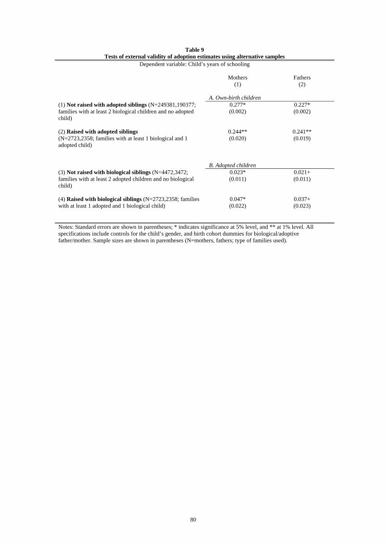
80

Table 9 Tests of external validity of adoption estimates using alternative samples

Dependent variable: Child’s years of schooling Mothers

(1) Fathers

(2) A. Own-birth children (1) Not raised with adopted siblings (N=249381,190377; families with at least 2 biological children and no adopted child)

0.277* (0.002)

0.227* (0.002)

(2) Raised with adopted siblings (N=2723,2358; families with at least 1 biological and 1 adopted child)

0.244** (0.020)

0.241** (0.019)

B. Adopted children (3) Not raised with biological siblings (N=4472,3472; families with at least 2 adopted children and no biological child)

0.023* (0.011)

0.021+ (0.011)

(4) Raised with biological siblings (N=2723,2358; families with at least 1 adopted and 1 biological child)

0.047* (0.022)

0.037+ (0.023)

Notes: Standard errors are shown in parentheses; * indicates significance at 5% level, and ** at 1% level. All specifications include controls for the child’s gender, and birth cohort dummies for biological/adoptive father/mother. Sample sizes are shown in parentheses (N=mothers, fathers; type of families used).

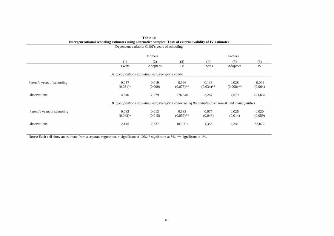
81

Table 10 Intergenerational schooling estimates using alternative samples: Tests of external validity of IV-estimates

Dependent variable: Child’s years of schooling

Mothers Fathers (1) (2) (3) (4) (5) (6)

Twins Adoptees IV Twins Adoptees IV A. Specifications excluding last pre-reform cohort Parent’s years of schooling

0.057 (0.031)+

0.019 (0.009)

0.196 (0.073)**

0.136 (0.034)**

0.028 (0.008)**

-0.009 (0.064)

Observations 4,840 7,579 276,346 3,247 7,579 221,637 B. Specifications excluding last pre-reform cohort using the samples from low-skilled municipalities Parent’s years of schooling

0.083 (0.043)+

0.013 (0.015)

0.183 (0.057)**

0.077 (0.048)

0.026 (0.014)

0.020 (0.059)

Observations 2,145 2,727 107,901 1,358 2,241 88,072 Notes: Each cell show an estimate from a separate regression. + significant at 10%; * significant at 5%; ** significant at 1%.

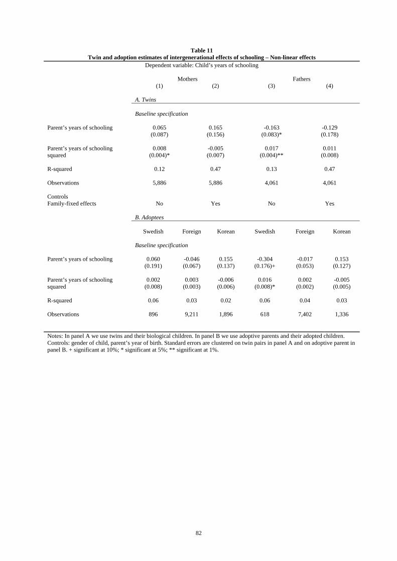
82

Table 11 Twin and adoption estimates of intergenerational effects of schooling – Non-linear effects

Dependent variable: Child’s years of schooling Mothers Fathers (1) (2) (3) (4) A. Twins

Baseline specification

Parent’s years of schooling

0.065 (0.087)

0.165 (0.156)

-0.163 (0.083)*

-0.129 (0.178)

Parent’s years of schooling squared

0.008 (0.004)*

-0.005 (0.007)

0.017 (0.004)**

0.011 (0.008)

R-squared 0.12 0.47 0.13 0.47 Observations 5,886 5,886 4,061 4,061 Controls Family-fixed effects No Yes No Yes B. Adoptees Swedish Foreign Korean Swedish Foreign Korean

Baseline specification

Parent’s years of schooling

0.060 (0.191)

-0.046 (0.067)

0.155 (0.137)

-0.304 (0.176)+

-0.017 (0.053)

0.153 (0.127)

Parent’s years of schooling squared

0.002 (0.008)

0.003 (0.003)

-0.006 (0.006)

0.016 (0.008)*

0.002 (0.002)

-0.005 (0.005)

R-squared 0.06 0.03 0.02 0.06 0.04 0.03 Observations 896 9,211 1,896 618 7,402 1,336 Notes: In panel A we use twins and their biological children. In panel B we use adoptive parents and their adopted children. Controls: gender of child, parent’s year of birth. Standard errors are clustered on twin pairs in panel A and on adoptive parent in panel B. + significant at 10%; * significant at 5%; ** significant at 1%.

83

Table 12 Income as a mechanism explaining the intergenerational transmission of schooling

Dependent variable: Child’s years of schooling Mothers Fathers

(1) (2) (3) (4) (5) (6) (7) (8) (9) (10)

Twins OLS

Twin-fixed

effects

Adoptees Reform sample OLS

Reform sample IV

Twins OLS

Twin-fixed

effects

Adoptees Reform sample OLS

Reform sample

IV A. Parent’s returns to schooling

Parent’s years of schooling 0.067

(0.004)** 0.047

(0.008)** 0.080

(0.003)** 0.082

(0.004)** 0.044

(0.018)* 0.062

(0.004)** 0.047

(0.008)** 0.069

(0.003)** 0.077

(0.003)** -0.004 (0.020)

B. The impact of parent’s log income on child’s schooling Parent’s log Income 0.613

(0.071)** 0.144

(0.114) 0.089

(0.039)* 0.670

(0.034)** --

0.910 (0.083)**

0.395 (0.148)**

0.097 (0.040)*

0.905 (0.031)**

--

Observations 5,795 5,795 8,087 271,790 271,790 4,054 4,054 6,576 220,946 220,946 Controls: Family-fixed effects No Yes No No No No Yes No No No Municipality-fixed effects No No No No Yes No No No No Yes Municipality*trend No No No No Yes No No No No Yes Notes: All columns include controls for gender of child and parent’s year of birth. Each estimate is from a separate regression. + significant at 10%; * significant at 5%; ** significant at 1%.

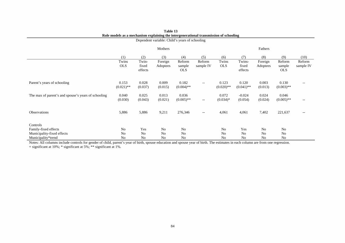
84

Table 13 Role models as a mechanism explaining the intergenerational transmission of schooling

Dependent variable: Child’s years of schooling Mothers Fathers

(1) (2) (3) (4) (5) (6) (7) (8) (9) (10)

Twins OLS

Twin-fixed

effects

Foreign Adoptees

Reform sample OLS

Reform sample IV

Twins OLS

Twins-fixed

effects

Foreign Adoptees

Reform sample OLS

Reform sample IV

Parent’s years of schooling 0.153

(0.021)** 0.028

(0.037) 0.009

(0.015) 0.182

(0.004)** -- 0.123

(0.020)** 0.120

(0.041)** 0.003

(0.013) 0.130

(0.003)** --

The max of parent’s and spouse’s years of schooling 0.040

(0.030) 0.025

(0.043) 0.013

(0.021) 0.036

(0.005)** -- 0.072

(0.034)* -0.024 (0.054)

0.024 (0.024)

0.046 (0.005)** --

Observations 5,886 5,886 9,211 276,346 -- 4,061 4,061 7,402 221,637 -- Controls Family-fixed effects No Yes No No No Yes No No Municipality-fixed effects No No No No No No No No Municipality*trend No No No No No No No No Notes: All columns include controls for gender of child, parent’s year of birth, spouse education and spouse year of birth. The estimates in each column are from one regression. + significant at 10%; * significant at 5%; ** significant at 1%.