1

The Causative Factors of Bangladesh’s Exports:

Evidence from the Gravity Model Analysis.

Mohammad Mafizur Rahman

Lecturer in Economics School of Accounting, Economics and Finance

Faculty of Business University of Southern Queensland

Toowoomba, QLD 4350, AUSTRALIA. Tel: 61 7 4631 1279 Fax: 61 7 4631 5594

Email: rahman@usq.edu.au Abstract: The paper firstly notes a theoretical justification for using the gravity model in the analysis of bilateral trade under either perfectly competitive or monopolistic market structure. It then applies a generalized gravity model to analyze Bangladesh’s export trade pattern using the panel data estimation technique. The estimated results reveal that the main contributors of the Bangladesh’s exports are the exchange rate, partner countries’ total import demand, openness of Bangladesh economy and multilateral resistance factors. All affects the country’s exports positively. Transportation costs affect Bangladesh’s exports negatively. The country specific effects show that neighbouring countries’ influence on Bangladesh’s exports is more than the influence of other distant countries. Keywords: Gravity Model, Panel Data, Fixed Effect Model, Bangladesh’s Exports. JEL Classification: C21, C23, F10, F11, F12, F14. Rahman, Mohammad Mafizur (2007) 'The Causative Factors of Bangladesh’s Exports: Evidence from the Gravity Model Analysis.' In: (The New Zealand Association of Economists 48th Annual Conference, 27-29 June, 2007, Christchurch, New Zealand) Author copy. Accessed from USQ ePrints: http://eprints.usq.edu.au

2

I. Introduction The foreign trade sector of Bangladesh constitutes an important part of its economy. The trade-GDP ratio increased to 36.88 percent in 2001 (World Bank 2004) from 16.41 percent in 1980 (World Bank 2001). However, despite its gradual importance, this sector has been suffering from a chronic deficit over the years. The trade relations of Bangladesh with other countries do not show any hopeful sign of them providing a desirable contribution to the country’s economic development. This is mainly due to low export trade of Bangladesh compared to its import trade. Therefore, it is essential to find out the determining factors of Bangladesh’s exports in order to help policy makers and planners to undertake appropriate measures to improve the trade performance. With this objective in mind this paper attempts to find out the major determining factors of Bangladesh’s exports using the panel data estimation technique and the generalized gravity model. The use of the gravity model to study international trade flows is now well established in economic literature. For more than four decades the model has been used by many researchers such as Tinbergen (1962), Pöyhönen (1963) and Linnemann (1966), Anderson (1979), Bergstrand (1985 and 1989), Helpman and Krugman (1985), Eaton and Kortm (1997), Deardorff (1998), Evenett and Keller (1998), Haveman and Hummels (2004) and others. Surveying the existing literature, in this research, we have argued that the use of the gravity model to analyse bilateral trade patterns is theoretically justified as the gravity equation can be derived assuming either perfect competition or monopolistic market structure. This model originates from the Newtonian physics notion. The gravity model of trade basically states that trade flows between two countries are determined positively by their income and negatively by the distance between them. This formulation can be generalized to Xij = αYi

βYjγDij

δ (1)

where Xij is the flow of exports from country i into country j , Yi and Yj are country i’s and country j’s GDPs and Dij is the geographical distance between the countries’ capitals; δ is expected to be negative.

The linear form of the model is as follows:

Log (Xij) = α + β log (Yi) + γ log (Yj) + δ log (Dij) (2) When estimated, this baseline model gives relatively good results. However, there are other factors that influence trade levels as well. Most estimates of gravity models add a certain number of dummy variables to (2) that test for specific effects, for example being a member of a trade agreement, sharing a common land border, speaking the same language and so on.

Assuming that we wish to test for p distinct effects (Gs), the model then becomes:

3

p Log (Xij) = α + β log (Yi) + γ log (Yj) + δ log (Dij) + Σ λsGs (3)

s=1 The main contributions of this paper are: it reaffirms a theoretical justification for using the gravity model in applied research of bilateral trade; it applies, for the first time, panel data approach in a gravity model framework to identify the determinants of Bangladesh’s export trade1.

The rest of the paper is organised as follows: section II presents theoretical justification of the model; section III analyses Bangladesh’s export trade using panel data and the gravity model; section IV looks at a sensitivity analysis of the model, and finally section V summarizes and concludes the paper. II. THEORETICAL JUSTIFICATIONS FOR APPLYING GRAVITY MODEL TO THE ANALYSIS OF TRADE PATTERNS The Newton’s gravity law is the first justification of the gravity model of trade. The second justification for the gravity equation can be analysed in the light of a partial equilibrium model of export supply and import demand as developed by Linneman (1966) (see Appendix 1 for Linneman’s approach). Based on some simplifying assumptions the gravity equation turns out, as Linneman argues, to be a reduced form of this model. However, Bergstrand (1985) and others point out that this partial equilibrium model could not explain the multiplicative form of the equation and also left some of its parameters unidentified mainly because of the exclusion of price variables. With the simplest form of the gravity equation, Linneman’s justification for exclusion of prices seems to be consistent (Jakab et al. 2001). Using a trade share expenditure system Anderson (1979) also derives the gravity model which postulates identical Cobb-Douglas or constant elasticity of substitution (CES) preference functions for all countries as well as weakly separable utility functions between traded and non-traded goods. The author shows that utility maximization with respect to income constraint gives traded goods shares that are functions of traded goods prices only. Prices are constant in cross-sections; so using the share relationships along with trade balance / imbalance identity, country j’s imports of country i’s goods are obtained. Then assuming log linear functions in income and population for traded goods shares, the gravity equation for aggregate imports is obtained (see Appendix 2). After considering the endogeneity between income and trade variables, Anderson (ibid.) follows the Instrumental Variable (IV) approach and thereby proposes two alternative solutions. Using different instruments either a lagged value of income can be used as instrument or first stage estimation of shares by OLS can be used and income values obtained from estimated shares can be substituted for a second stage

1 Hassan (2000, 2001 and 2002) examines the effects of regional trade block on bilateral trade of 27 countries using cross sectional data. Hence his study is different from the current one.

4

re-estimation of the gravity equation. For many goods, the aggregate gravity equation is obtained only by substituting a weighted average for the actual shares in the second stage (Krishnakumar 2002). The third justification for the gravity model approach is based on the Walrasian general equilibrium model, with each country having its own supply and demand functions for all goods. Aggregate income determines the level of demand in the importing country and the level of supply in the exporting country (Oguledo and Macphee 1994). While Anderson’s (ibid.) analysis is at the aggregate level, Bergstrand (1985, 1989) develops a microeconomic foundation to the gravity model. He opines that a gravity model is a reduced form equation of a general equilibrium of demand and supply systems. In such a model the equation of trade demand for each country is derived by maximizing a constant elasticity of substitution (CES) utility function subject to income constraints in importing countries. On the other hand, the equation of trade supply is derived from the firm’s profit maximization procedure in the exporting country, with resource allocation determined by the constant elasticity of transformation (CET). The gravity model of trade flows, proxied by value, is then obtained under market equilibrium conditions, where demand for and supply of trade flows are equal. (Karemera et al. 1999). Bergstrand argues that since the reduced form eliminates all endogenous variables out of the explanatory part of each equation, income and prices can also be used as explanatory variables of bilateral trade. Thus instead of substituting out all endogenous variables, Bergstrand (ibid.) treats income and certain price terms as exogenous and solves the general equilibrium system retaining these variables as explanatory variables. The resulting model is termed a “generalized” gravity equation (Krishnakumar 2002). Bergstrand’s analysis is based on the assumptions of nationwide product differentiation by monopolistic competition and identical preferences and technology for all countries. With N countries, one aggregate tradable good, one domestic good and one internationally immobile factor of production in each country, Bergstrand’s (1985) model becomes a general equilibrium model of world trade. Bergstrand’s (1989) later model is an extension of his earlier work. In this model production is added under monopolistic competition among firms that use labour and capital as factors of production. Firms are assumed to produce differentiated products under increasing returns to scale. Based on some simple assumptions on taste and technology Bergstrand again derives the general form of the gravity equation. The micro-foundations approach also alleges that the crucial assumption of perfect product substitutability of the ‘conventional’ gravity model is unrealistic as recent evidence shows that trade flows are differentiated by place of origin. So exclusion of price variables leads to misspecification of the gravity model. Anderson (1979), Bergstrand (1985, 1989), Thursby and Thursby (1987), Helpman & Krugman (1985) and others share this view. These studies show that price variables, in addition to the conventional gravity equation variables, are also statistically significant in explaining trade flows among participating countries (Oguledo and Macphee 1994). Generally a commodity moves from a country where prices are low to a country where prices are high. Therefore, export trade flows are positively related to changes in export prices, and import trade flows are negatively related to changes in import prices (Karemera et al. 1999). Hence prices of a particular commodity in trading countries are important. However, price and exchange rate variables can be omitted only when products are perfect substitutes in consumer preferences and when they can be transported without

5

cost between markets, which are the basic assumptions behind the standard Heckscher-Ohlin (H-O) model (Jakab 2001). Eaton and Kortum (1997) also derive the gravity equation from a Ricardian framework, while Deardorff (1998) derives it from a H-O perspective. Deardorff opines that the H-O model is consistent with the gravity equations. He argues that gross trade flows will follow a gravity equation if trade is frictionless, producers and consumers are indifferent and markets are settled randomly among all possibilities. Deardorff also proves that, if trade is impeded and each good is produced by only one country, the H-O framework will result in the same bilateral trade pattern as the model with differentiated products. If there are transaction costs of trade, distance should also be included in the gravity equation. As shown by Evenett and Keller (1998), the standard gravity equation can be obtained from the H-O model with both perfect and imperfect product specialization. Some assumptions different from increasing returns to scale, of course, are required for the empirical success of the model (Jakab et al. 2001). Economies of scale and technology differences are the explanatory factors of the comparative advantage instead of considering factor endowment as a basis of this advantage as in the H-O model (Krishnakumar 2002). Evenett and Keller (ibid) note that the volume of trade is determined by the extent of product specialization, and argue that the increasing returns to scale model rather than the perfect specialization version of the H-O model is more likely to be a candidate for explaining the success of the gravity equation. Furthermore, they reveal that models with imperfect product specialization, compared to models with perfect product specialization, can explain variations better in the volume of trade. Extending this analysis Feenstra et al. (2001) observe that when tested within the differentiated product category the monopolistic competition models of international trade account for the success of the equation (Carrillo and Li 2002). Haveman and Hummels (2001 and 2004) note that the gravity equation can be generated from a model with complete and incomplete specialization (see Appendix 3). The works of Anderson (1979), Bergstrand (1985), Deardorff (1998), and Helpman and Krugman (1985) are examples of complete specialization model. Derivation of the gravity equation under the complete specialization model implies that each good is produced in only one country; consumers highly value variety and therefore import all goods that are produced. On the other hand, the incomplete specialization model implies that importers buy from only a small fraction of available sources. As a result, trade levels predicted under the complete specialization model are much higher than the incomplete specialization model (Haveman and Hummels 2004). To test for the relevance of monopolistic competition in international trade Hummels and Levinsohn (1993) use intra-industry trade data. Their results show that much intra-industry trade is specific to country pairings. So their work supports a model of trade with monopolistic competition (Jakab et al. 2001). Therefore, the gravity equation can be derived assuming either perfect competition or a monopolistic market structure. Also neither increasing returns nor monopolistic competition is a necessary condition for its use if certain assumptions regarding the structure of both product and factor market hold (Jakab et al. 2001).

6

Analysing the theoretical foundations of gravity equations, Evenett and Keller (1998) mention three types of trade models. These models differ in the way specialisation is obtained in equilibrium. They are:

(1) technology differences across countries in the Ricardian model, (2) variations in terms of countries’ different factor endowments in the H-O

model, (3) increasing returns at the firm level in the model of Increasing Returns to Scale

(IRS). These are the perfect specialization models, and are considered as limiting cases for a model of imperfect specialisation. But empirically imperfect product specialisation is important. In real life, though technologies and factor endowments are different in different countries, they change over time and can be transferred between countries. Trade theories just explain why countries trade in different products but do not explain why some countries’ trade links are stronger than others and why the level of trade between countries tends to increase or decrease over time. This is the limitation of trade theories in explaining the size of trade flows. Therefore, while traditional trade theories cannot explain the extent of trade, the gravity model is successful in this regard. It allows more factors to be taken into account to explain the extent of trade as an aspect of international trade flows (Paas 2000). Trade occurs because of differences across countries in technologies (Ricardian theory), in factor endowments (H-O theory), differences across countries in technologies as well as continuous renewal of existing technologies and their transfer to other countries (Posner 1961 and Vernon 1966). Quoting from Dreze (1961), Mathur (1999) says that country size and scale economies are important determinants of trade (Paas 2000). Production will be located in one country if economies of scale are present. Economies of scale also induce producers to differentiate their product. The larger the country is in terms of its GDP/GNP, for instance, the larger the varieties of goods offered. The more similar the countries are in terms of GDP/ GNP, the larger is the volume of this bilateral trade. Thus with economies of scale and differentiated products, the volume of trade depends in an important way on country size in terms of its GDP/GNP (Paas 2000). This is the concept of new theories of international trade,2 and it provides a better explanation of the empirical facts of international trade in terms of their pattern, direction and rate of growth. As a result, the traditional trade theories have been supplemented, if not replaced, by the new trade theories in recent years, based on the assumption of product differentiation and economies of scale. The H-O and Ricardian theories of trade contradict with trade in the real world. In the H-O model the larger the differences in the factor endowments between two countries, the larger will be the trade. Therefore, based on this ground we would expect little trade between the developed countries of Western Europe since these

2 Among the contributors of these new theories, Krugman (1979), Lancaster (1980), Helpman (1981, 1984, 1987 and 1989), Helpman and Krugman (1985, 1989), and Deardorff (1984) warrant special mention in the context of their explaining trade both empirically and theoretically (Mathur 1999). These theories implicitly assume similar technologies and factor endowments across countries (Pass 2000).

7

countries have similar factor endowments and more trade between developing and developed countries. This is contrary to empirical fact. This is evident from the international trade statistics that both intra-industry trade and trade between developed countries are conspicuously large. Linder’s (1961) hypothesis of trade seems to be more relevant in real life. This hypothesis suggests that the presence of increasing returns in production causes the production of each good to be located in either of the countries but not in both of them. It is also suggested that countries with similar per capita income will have a similar demand structure. So the more similar the countries are in per capita income, the larger is likely to be their bilateral trade. That is, the “absolute value of the difference” of per capita income in any two countries will have a negative effect on their bilateral trade. This should explain the trade pattern between developed countries (Mathur 1999). However, Deardorff (1998) argues that a certain kinship to Heckscher-Ohlin can be viewed in the gravity model. According to the H-O theory, capital intensive goods are produced by capital-rich countries. So, as Markusen (1986) has already shown, if high- income consumers tend to consume larger budget shares of capital intensive goods, then it follows that (1) capital rich countries will trade more with other capital rich countries than with capital poor countries, and (2) capital poor countries will trade more with their own kind. These are the same predictions as those of the Linder hypothesis (Frankel 1997). From the discussion above it is clear that there are two views of trade theorems: supply side and demand side. Differences in technology, factor endowments, economies of scale, etc., are the supply side theorems of trade. On the other hand, Linder’s hypothesis and intra-industry trade are the demand side explanations of trade. The use of the gravity model in analyzing the bilateral trade flows is a good choice as it contains elements of both demand and supply side explanations of trade. While GNP is being taken as a variable, the reason for taking ‘per capita GNP’ as a separate independent variable is that it indicates the level of development. If a country develops, consumers demand more exotic foreign varieties that are considered superior goods. Further, the process of development may be led by the innovation or invention of new products that are then demanded as exports by other countries. Also it is true that more developed countries have more advanced transportation infrastructures which facilitate trade. Transportation cost is an important factor of trade. Production of the same good in two or more countries in the presence of transport costs is inconsistent with factor price equalization. Moreover, different trade models might behave differently in the presence of transport cost and differences in demand across countries (Paas 2000, quoted from Davis and Weinstein 1996). Transport costs are proxied by distance. So distance between a pair of countries naturally determines the volume of trade between them. Studies based on a general equilibrium approach, (Tinbergen 1962, Pöyhönen 1963, Bergstrand 1985, 1989 etc.) conclude that incomes of trading partners and the distances between them are statistically significant and expect positive and negative signs, respectively (Oguledo

8

and Macphee 1994, Karemera et al. 1999). Three kinds of costs are associated with doing business at a distance: (i) physical shipping costs, (ii) time-related costs and (iii) costs of (cultural) unfamiliarity. Among these costs, shipping costs are obvious (Frankel 1997 quoted from Linneman 1966). The majority of the general equilibrium studies have found the population sizes of the trading countries to have a negative and statistically significant effect on trade flows (Linneman 1966, Sapir 1981, Bikker 1987) although a few exceptions have also been found in literature (Brada and Mendez 1983 for example). Trade barriers such as tariffs have a statistically significant negative effect on trade flows between countries. On the other hand, preferential arrangements are found to be trade enhancing and statistically significant (Oguledo and Macphee 1994). The reason is that trade group member countries are more likely to have incentives for trade with each other as their cultures or cultural heritages and patterns of consumption and production are likely to be similar. Also countries with common borders are likely to have more trade than countries without common borders (Karemera et al. 1999). III. APPLICATION OF THE GRAVITY MODEL IN ANALYZING BANGLADESH’S EXPORT TRADE A Brief Picture of the Bangladesh’s Trade As mentioned earlier, the trade sector is continuously playing an important role in the Bangladesh economy. In 1999, compared to 1988, Bangladesh’s total trade, total exports and total imports increased by 168%, 204% and 153% respectively. In the case of trade with our sample countries, this increase is the highest for the SAARC countries 439% (exports + imports). When separated, the increase of imports is the highest for the SAARC countries (602%), followed by ASEAN (276%) and EEC (107%); the increase of exports is the highest for the EEC countries (363%) followed by the NAFTA countries (323%), the Middle East countries (85%) and the SAARC countries (33%). Individually, in 1999, 20% of Bangladesh’s trade of our sample total occurred with the USA followed by India (12%), UK, Singapore, Japan (7%), and China, Germany (6%). In the same year the exports figures of Bangladesh are, of our sample total, 39% to the USA, 12% to Germany, 10% to UK, 7% to France, 5% to the Netherlands and Italy, 2% to Japan, Hong Kong, Spain and Canada and 1% to India and Pakistan. On the other hand, the imports figure of Bangladesh, of our sample total, is the highest from India (18%) followed by Singapore (12%), Japan (10%), China (9%) and USA and Hong Kong 8%. The over all trade balance of Bangladesh, of course, gives us disappointing results. Compared to 1988, the total trade deficit of Bangladesh increased by 115% in 1999. This figure is 987% with the SAARC countries, 1098% with India and 108% with Pakistan (IMF: Direction of Trade Statistics Yearbook, various years). Sample Size and Data Issues Our study covers a total of 35 countries. The countries are chosen on the basis of importance of trading partnership with Bangladesh and the vailability of required data. Five countries from SAARC, five countries from ASEAN, three countries from NAFTA, eleven countries from the EEC (EU) group, six countries from the Middle East and five Other countries are included in our sample for the analysis of Bangladesh’s trade3.

3 SAARC: Bangladesh, India, Nepal, Pakistan and Sri Lanka; ASEAN: Indonesia, Malaysia, the Philippines, Singapore and Thailand; NAFTA: Canada, Mexico and USA; EU: Belgium, Denmark, France, Germany, Greece, Italy, the Netherlands, Portugal, Spain, Sweden and the United Kingdom; Middle East: Egypt, Iran, Kuwait, Saudi Arabia, Syrian Arab Republic and the United Arab Emirates; Other: Australia, New Zealand, Japan, China and Hong Kong.

9

The data were collected for the period of 1972 to 1999 (28 years). All observations are annual. Data on GNP, GDP, GNP per capita, GDP per capita, population, inflation rates, total exports, total imports and CPI are obtained from the World Development Indicators (WDI) database of the World Bank. Data on exchange rates are obtained from the International Financial Statistics (IFS), CD-ROM database of International Monetary Fund (IMF). Data on Bangladesh’s exports of goods and services (country i’s exports) to all other countries (country j), Bangladesh’s imports of goods and services (country i’s imports) from all other countries (country j) and Bangladesh’s total trade of goods and services (exports plus imports) with all other countries included in the sample are obtained from the Direction of Trade Statistics Yearbook (various issues) of IMF. Data on the distance (in kilometer) as the crow flies between Dhaka (the capital of Bangladesh) and other capital cities of country j are obtained from an Indonesian Website: www.indo.com/distance. GNP, GDP, GNP per capita, GDP per capita are in constant 1995 US dollars. GNP, GDP, total exports, total imports, taxes, Bangladesh’s exports, Bangladesh’s imports and Bangladesh’s total trade are measured in million US dollars. The population of all countries are considered in million. GNP and per capita GNP of the U.K. and New Zealand are always replaced by GDP and per capita GDP of these two countries respectively as the data on the former are not available for some years of the sample period. Data on the exchange rates are available in national currency per US dollar for all countries; so these rates are converted into the country j’s currency in terms of Bangladesh’s currency (country i’s currency). Methodology Classical gravity model generally uses cross-section data to estimate trade effects and trade relationships for a particular time period, for example one year. In reality, however, cross-section data observed over several time periods (panel data methodology) result in more useful information than cross-section data alone. The advantages of this method are: firstly, panels can capture the relevant relationships among variables over time; and secondly, panels can monitor unobservable trading-partner-pairs’ individual effects. If individual effects are correlated with the regressors, OLS estimates omitting individual effects will be biased. Therefore, we have used panel data methodology for our empirical gravity model of export trade.

The generalized gravity model of export trade states that the volume of exports of country i to country j, Xij, is a function of their incomes (GNPs or GDPs), their populations or per capita income, their distance (proxy of transportation costs) and a set of dummy variables either facilitating or restricting trade between pairs of countries. That is, Xij = β0 Yi

β1 Yjβ2

yiβ3 yj

β4 Dij

β5 Aijβ6 Uij (4)

where Yi (Yj) indicates the GDP or GNP of the country, i (j), yi (yj) are per capita income of country, i (j), Dij measures the distance between the two countries’ capitals (or economic centers), Aij represents dummy variables, Uij is the error term, and βs are parameters of the model. As the gravity model is originally formulated in multiplicative form, we can linearize the model by taking the natural logarithm of all variables. So for estimation purposes, model (4) in log-linear form in year t, is expressed as, lXijt = β0 + β1lYit + β2lYjt +β3lyit +β4lyjt +β5lDijt + ∑δhPijht + Uijt (5) h

where l denotes variables in natural logs and Pijh is a sum of preferential trade dummy variables. The dummy variable takes the value one when a certain condition is satisfied, zero otherwise.

10

Adding some more independent variables4 in our model (5) we consider the following gravity model of Bangladesh’s exports: lXijt = β0 + β1lYit + β2lYjt +β3lyit +β4lyjt +β5lDijt + β6lydijt +β7lERijt+ β8lInit+ β9lInjt+ β10lTEit + β11lTIjt + β12(IM/Y)jt + β13(TR/Y)it +β14(TR/Y)jt+ ∑δhPijht + Uijt (6) h

where, X= exports, Y=GDP, y = per capita GDP, D= distance, yd= per capita GDP differential, ER = exchange rate, In = inflation rate, TE = total export, TI =total import, IM/Y = Import-GDP ratio, TR/ Y= trade-GDP ratio, P =preferential dummies. Dummies are: D1= j-SAARC, D2=j-ASEAN, D3= j-EEC, D4 = j-NAFTA, D5= j-Middle East, D6 = j- others and D7= borderij, l= natural log.

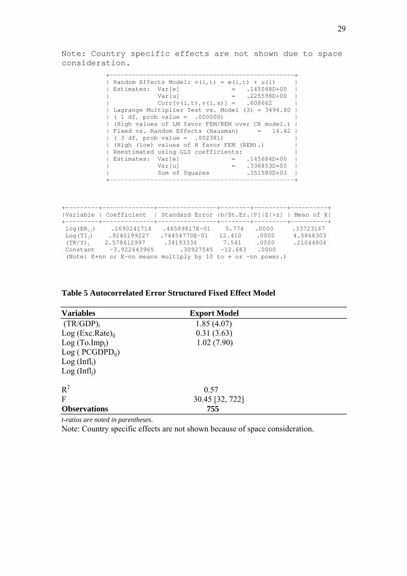
In our estimation, we have used unbalanced panel data, and individual effects are included in the regressions. Therefore, we have to decide whether they are treated as fixed or as random. From the regression results of the panel estimation, we get the results of LM test and Hausman test [in the REM of Panel estimation]. These results5 suggest that FEM of panel estimation is the appropriate model for our study.

There is, of course, a problem with FEM. We cannot directly estimate variables that do not change over time because inherent transformation wipes out such variables. Distance and dummy variables in our aforesaid models are such variables. However, this problem can easily be solved by estimating these variables in a second step, running another regression with the individual effects as the dependent variable and distance and dummies as independent variables,

IEij= β0 +β1Distanceij +∑δhPijh + Vij (7)

h

where IEij is the individual effects.

Estimates of Gravity Equations, Model Selection and Discussion of results

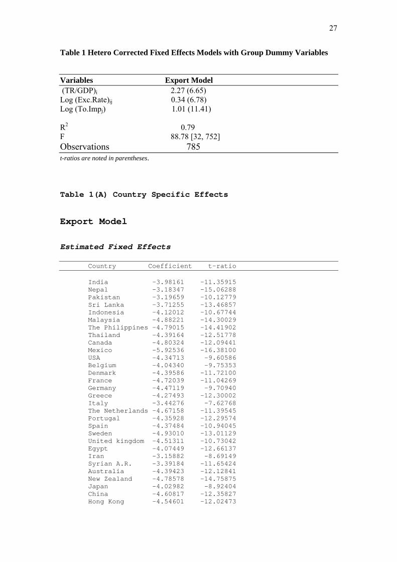
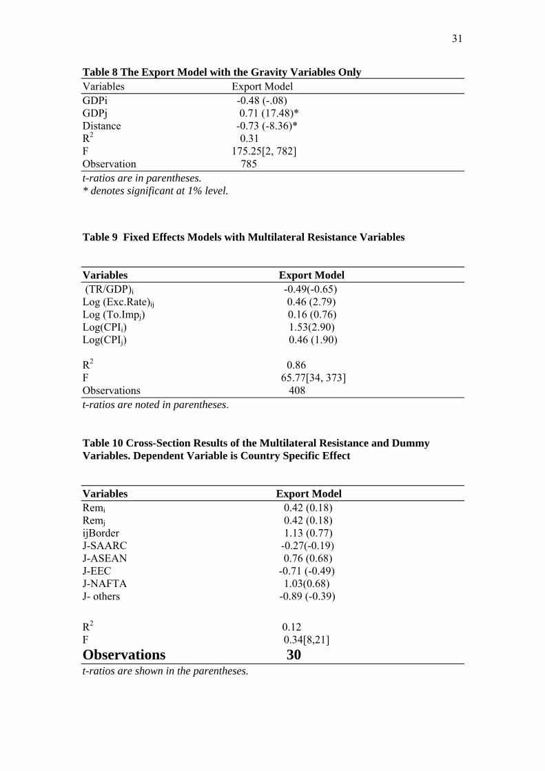
Estimation and Model selection The gravity model of Bangladesh’s exports-equation (6) above- has been estimated taking all explanatory variables except the distance and dummy variables for 785 observations of 31 countries. Many variables are found to be either insignificant or possessed wrong signs. In the process of model selection, we have found only GDPi, exchange rateij, total importj, import/GDPj, trade/GDPi are found to be significant. When tested for the multicollinearity of the variables, GDPi is found to have multicollinearity problem. Dropping this variable if we re-estimate the model on the remaining four variables, it is found that the variable import / GDPj is insignificant. So our estimated desired model is now: lXijt = β0 + β7lERijt+ β11lTIjt + β13(TR/Y)it (6’) Now all explanatory variables are found to be significant with expected signs. The results of the heteroscedasticity corrected model are shown in Table 1. The autocorrelated error structured model is also noted in Table 5.

4 Explanatory variables are selected on the basis of past literature and economic implications that affect export trade. 5 Results are not shown. However, these can be provided upon request.

11

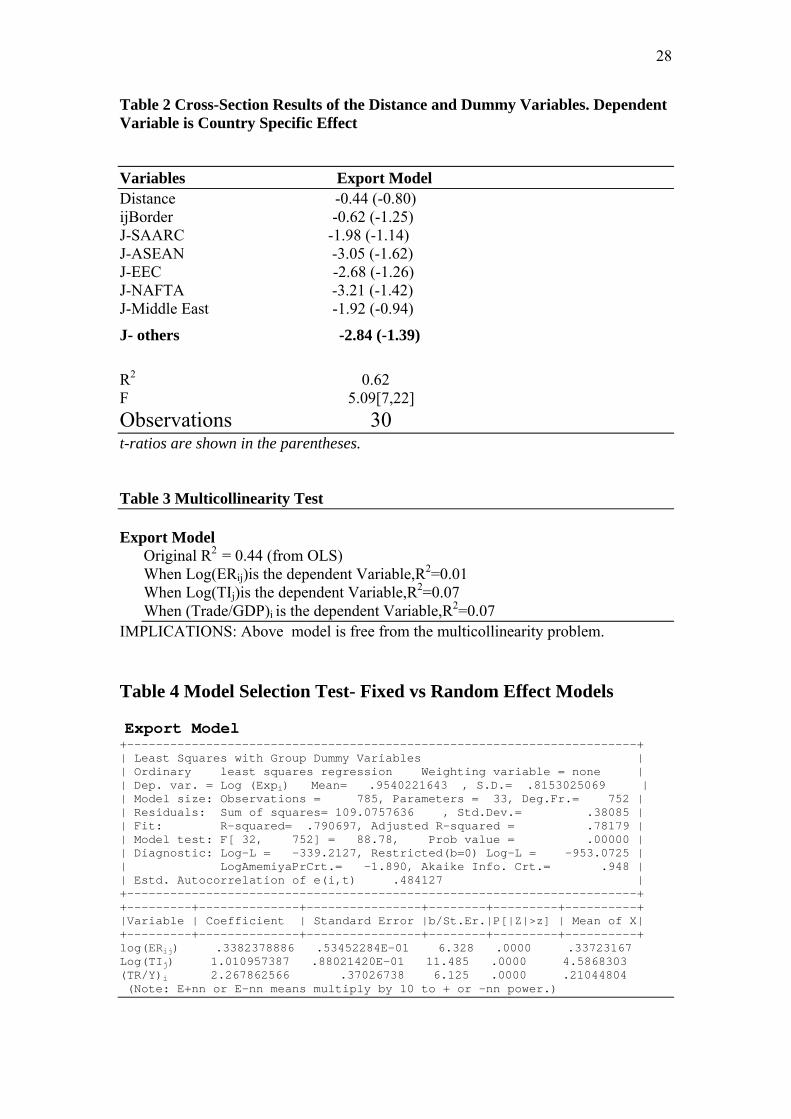
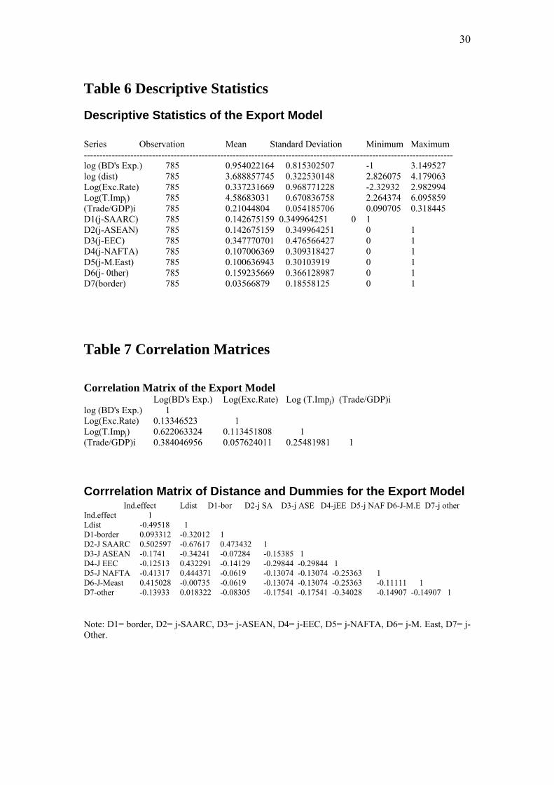
The results for the multicollinearity test are noted in Table 3. From the results it can be observed that the model does not have any multicollinearity problem. The estimation results of unchanged variables for equation (6) above -that is equation (7) - are noted in Table 2. The country specific effects of the heteroscedasticity corrected model are shown in Table 1(A). The test for the appropriateness of the FEM in the analysis is shown in Table 4. Table 6 shows the descriptive statistics of the model; Table 7 presents the correlation matrices of these models and Table 8 gives the results of the gravity variables only.

Endogeneity Issue

As mentioned earlier, Bergstrand (1985, 1989) argues that income (size of the economy) can be treated as an exogenous variable in the gravity model, as a gravity model is a reduced form equation of a general equilibrium of demand and supply systems, and the reduced form eliminates all endogenous variables out of the explanatory part of each equation. However, there is empirical and theoretical support that trade can also affect income. If an endogeneity problem exists, the effect of income on trade may be misleading. To solve this problem alternative instrumental variables (IV) estimations, as suggested by Anderson (1979), were attempted using lagged value of income and population as instruments. This alternative estimation does not change the coefficient of any of the variables to any significant extent. This implies that the endogeneity of income, if exists at all, does not create any significant distortion on the initially postulated relationship in the gravity model. Therefore, GNP and GNP per capita are treated as exogenous variables in the estimation.

Discussion of Results As mentioned earlier, all three of our gravity models suggest that, based on the LM and Hausman tests, FEM of Panel estimation is the appropriate strategy to be adopted. So the results of FEM will be discussed here for the said three models. The estimation uses White’s heteroskedasticity-corrected covariance matrix estimator. In these models, the intercept terms α0i and β0i are considered to be country specific, and the slope coefficients are considered to be the same for all countries. For the export model (Table 1), as mentioned earlier, only the variables exchange rate, total import of country j and the trade- GDP ratio of Bangladesh are found to be highly significant (even at the 1% level). The positive coefficient of the exchange rate implies that Bangladesh’s exports depend on its currency devaluation. From the estimated results it is evident that 1% currency devaluation leads to, other things being equal, 0.34% exports to j countries. Total imports of country j may be considered as the target country effect. The coefficient value of this variable is found to be large and carries an anticipated positive sign. The estimated results show that the exports of Bangladesh increase slightly higher than proportionately with the increase of total imports demand of country j. (The coefficient is: 1.01). The trade-GDP ratio of Bangladesh, the openness variable, has an expected positive sign. The coefficient of this variable is very large and indicates that Bangladesh has

12

to liberalise its trade barriers to a great extent for increasing its exports. The estimated coefficient is 2.27, which implies that Bangladesh’s exports increase 9.68% [exp (2.27) = 9.68] with 1% increase in its trade-GDP ratio, other things being equal. As far as country specific effects are concerned, all effects are highly significant [Table 1(A)]. The results show that Mexico followed by Sweden, Canada, New Zealand, France, the Netherlands, etc., have the lowest propensity to Bangladesh’s exports, and Nepal followed by Pakistan, Iran, Syrian, A.R., Italy, Sri Lanka, India, etc., have the highest propensity to Bangladesh’s exports. The model has R2 = 0.79, and F [32, 752]= 88.78. Also there is no multicollinearity problem among the variables. Almost similar results are obtained from the autocorrelated error structured model (Table 5) in terms of magnitude and the sign of coefficients. Interestingly the distance variable is found to be insignificant but has an expected negative sign (see Table 2). All dummy variables are found to be insignificant. Multilateral Resistance Factors Bilateral trade may be affected by multilateral resistance factors. Anderson and Wincoop (2003), Baier and Bergstrand (2003), and Feenstra (2003) have recently considered these factors in their works. Assuming identical, homothetic preferences of trading partners and a constant elasticity of the substitution utility function Anderson and Wincoop (2003) define multilateral trade resistance as follows: Pj = [∑(βipitij)1-σ] 1/(1- σ) (8) i where Pj is the consumer price index of j. βi is a positive distribution parameter, pi is country i’s (exporter’s) supply price, net of trade costs, tij is the trade cost factor between country i and country j, σ is the elasticity of substitution between all goods. For simplification they assume that the trade barriers are symmetric, that is, tij=tji. They refer to the price index (Pi or Pj) as multilateral trade resistance as it depends positively on trade barriers with all trading partners. High trade barriers for country i, reflected by high multilateral resistance Pi, lower demand for country i’s goods, reducing its supply price pi. Assuming σ >1, consistent with empirical results in the literature, it is easy to see why higher multilateral resistance of the importer j raises its trade with i. For a given bilateral barrier between i and j, higher barriers between j and its other trading partners will reduce the relative price of goods from i and raise imports from i. Trade would also be increased for the higher multilateral resistance of the exporter i. For a given bilateral barrier between i and j, trade would increase between them as higher multilateral resistance leads to a lower supply price pi. The authors also opine that trade between countries is determined by relative trade barriers. Trade volume between two countries depends on the bilateral barrier between them relative to average trade barriers that both countries face with all their trading partners (tij / PiPj). A rise in multilateral trade resistance implies a drop in relative resistance tij / PiPj, Multilateral trade resistance is not much affected for a large

13

country because the increased trade barriers do not apply to trade within the country, but for a very small country increased trade barriers lead to a large increase in multilateral resistance. To calculate tij (unobservable) the authors hypothesize that tij is a log linear function of observables: bilateral distance dij and whether there is an international border between i and j. The language variable can also be used as a dummy variable to determine the trade costs. Baier and Bergstrand (2003) note that the nonlinear estimation technique for the multilateral resistance factor in Anderson and van Wincoop (2003) is complex. Because accounting for the roles of multilateral price terms such as pi

g, pjg, Pi

g, and Pjg

has always been a difficult issue empirically, as no such data exist. They have used proxies for these multilateral terms. GDP weighted average of distance from trading partners can be used as a proxy for the multilateral resistance term. Feenstra (2003) mentions that once transportation costs or any other border barriers are introduced then prices must differ internationally. Therefore, overall price indexes in each country must be taken into account. This could be done in three ways. (1) Using published data on price indexes, (2) using the computational method of Anderson and van Wincoop (2003) or (3) using country fixed effects to measure the price indexes. Application of Multilateral Resistance in Bangladesh’s Exports We have re-estimated the gravity model for Bangladesh’s export [equation (6’)] adding CPI of trading partners as multilateral resistance variable. Here total observations are only 408 [Earlier the number of observations was 785]. Multilateral resistance variables are found to be significant though two other variables- total import of country j and trade-GDP ratio of country i-are found to be insignificant. The reason for these two variables being insignificant may be due to the small sample as stated above. The CPI variable has a positive effect on Bangladesh’s exports (see Table 9). This is expected, as the more there is multilateral resistance, the more the bilateral trade will be. However, when GDP weighted average of distance is taken as a multilateral resistance variable, we find the opposite (insignificant) result of this variable in our Export Model. McCallum (1995) considers remoteness as multilateral resistance. His definition for remoteness for country i, which is considered for estimation, is as follows: REMi = Σdim / ym (9) m≠ j This variable tends to reflect the average distance of region i from all trading partners other than j. This result has been obtained from OLS as the FEM for distance and dummy variables cannot be estimated. Taking the GDP weighted average of distance as a multilateral resistance variable the gravity equation of export model is re-estimated; it is found that this variable is insignificant in determining Bangladesh trade. The estimated results of the export model, when the multilateral resistance variable is considered in alternative ways, are noted in Table 5.10. From the F–value and R2-value, it can be said that model in Table

14

5.9 are satisfactory, and hence CPI is the acceptable multilateral resistance variable for the analysis of Bangladesh trade. IV. Sensitivity Analysis of the Model For the sensitivity analysis of the gravity model the methodology of Levine and Renelt (1992) and Yamarik and Ghosh (2005) is followed. With the help of extreme –bounds sensitivity analysis the robustness of coefficient estimates can be tested. In the sensitivity analysis, three kinds of explanatory variables are generally identified. They are labeled as I variables, M variables and Z variables. I is a set of variables always included in the regression (set of core variables), M is the variable of interest, Z is a subset of variables chosen from a pool of variables identified by past studies as potentially important explanatory variables. So if T denotes bilateral export trade, the equation for the sensitivity analysis of the gravity model of trade would be as follows: T = β0 + βi I + βm M + βz Z + u (10) where u is a random disturbance term. In the sensitivity analysis, first a “base” regression for each M variable is run including only the I –variables and the variable of interest as regressors. That is, the above equation (10) is estimated for each M variable imposing the constraint βz = 0. Then regression is made of T on the I, M and all Z variables (or all estimating combinations of the Z variables taken two at a time) and identification is made of the highest and lowest values for the coefficient on the variable of interest, βm, which is significant. Thus these are defined as the extreme upper and lower bounds of βm. If βm remains significant and of the same sign at each of the extreme bounds, then a fair amount of confidence can be maintained in that partial correlation, and thus the result can be referred to as “robust”. If βm does not remain significant or if it changes sign at one of the extreme bounds, then one might feel less confident in that partial correlation, and thus the result can be referred to as “fragile”. Estimation Strategy The estimation strategy must account for the cross-sectional and time-series information in the data in order to make optimal use of the available data. One approach could be that all the observations would be treated as equal and a pooled model would be estimated using OLS. A constant coefficient across time is the requirement for this strategy. An alternative approach could be that one could allow for country-pair heterogeneity in the regression, and this heterogeneity could be incorporated either through bilateral country-specific effects or individual country-specific effects. However, through the inclusion of country specific effects one cannot estimate many time-invariant variables like distance, common border, etc. Since the objective for sensitivity analysis is to test the robustness of the variables, including those that are time-invariant, the first estimation strategy6 was therefore chosen.

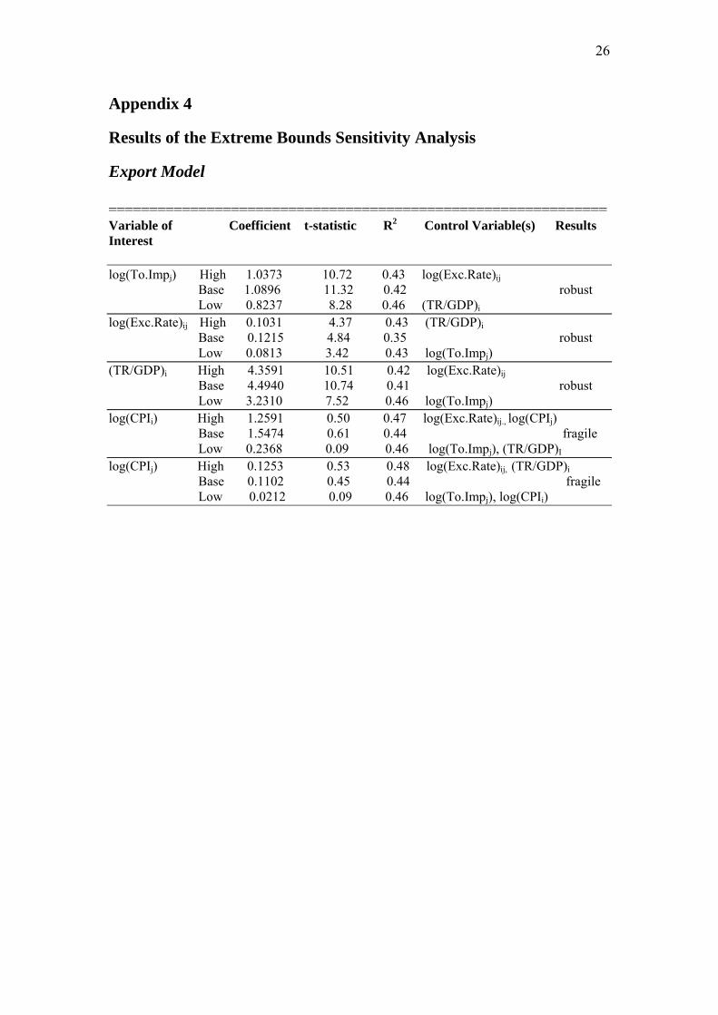
Results of the Sensitivity Analysis The results of the sensitivity analysis have been presented in Appendix 4. The appendix shows the results of 5 variables of interest under Export Model. For each 6 Yamarik and Ghosh (2005) also followed this strategy.

15

variable, three regression results are reported. These are the base model, the extreme upper bound and the extreme lower bound. The regression results include the estimated coefficient (estimated βm), the t-statistics, the R-squared and the controlled variables, Z, included in each regression. The Extreme Bound Analysis result- fragile or robust- of each variable of interest is reported in the last column.

All variables except the multilateral resistance variables are found to be robust. Both CPIi and CPIj variables are found to be fragile.

V. SUMMARY AND CONCLUSIONS The application of the gravity model in applied research of bilateral trade is theoretically justified. There are wide ranges of applied research where the gravity model is used to examine the bilateral trade patterns and trade relationships. Our results show that the major determinants of Bangladesh’s exports are: the exchange rate, the partner countries’ total import demand and the openness of the Bangladesh economy. All three factors affect Bangladesh’s exports positively. The country specific effects imply that Bangladesh would do better if the country trades more with its neighbours. Bangladesh’s exports are also positively related to multilateral resistance factors.

The policy implications of the results obtained are that all kinds of trade barriers in countries involved, especially in Bangladesh, must be liberalized to a great extent in order to enhance Bangladesh’s trade. It seems that Bangladesh’s currency is overvalued. Necessary devaluation of the currency is required to promote the country’s exports taking other adverse effects of devaluation, such as domestic inflation, into account. Proper quality of the goods and services must be maintained and the varieties of goods and service must be increased as the Bangladesh’s exports largely depend on the foreign demand. All partner countries’ propensities to export and import must be taken into account sufficiently and adequately when trade policy is set as the Bangladesh’s trade is not independent of country specific effects.

16

Appendix 1 The Trade Flow Model: Linneman Approach Factors contributing to trade flow between any pair of countries- say, the exports from country A to country B- may be classified in three categories. For example,

1. factors that indicate total potential supply of country A- the exporting country- on the world market;

2. factors that indicate total potential demand of country B- the importing country-

on the world market;

3. factors that represent the “resistance” to a trade flow from potential supplier A to potential buyer B.

The “resistance” factors are cost of transportation, tariff wall, quota, etc. The potential supply of any country to the world market is linked systematically to (i) the size of a country’s national or domestic product (simply as a scale factor), and

(ii) the size of a country’s population.

The level of a country’s per capita income may also be considered as a third factor though its influence will be very limited, at most. If the third factor indeed had no effect at all, then the factors (i) and (ii) would obviously be completely independent of each other as explanatory variables, on theoretical grounds. On the other hand, if the third factor did have an effect, then the three explanatory factors would not be independent of each other, as a change in one of the three would necessarily be associated with a change in at least one of the other two variables. For statistical exercises this has important implications because it would imply certain problems of identification. The Price Level Potential supply and potential demand, in the equilibrium situation, on the world market have to be equal. For this, a prerequisite must be that the exchange rate has been fixed at a level corresponding with the relative scarcity of the country’s currency on the world market. Equality of supply and demand on the world market also implies that every country has a moderate price level in the long run. If the price level is too high or too low, there would be a permanent disequilibrium of the balance of payments. Adjustment through a change in the exchange rate will necessarily take place. Therefore, the general price level will not influence a country’s potential foreign supply and demand except in the short-run. A Formula for the Flow of Trade Between Two Countries

17

Let Ep = Total potential supply Mp = Total potential demand R = Resistance Apparently the trade flow from country i to country j will depend on Ei

p and Mjp . We

assume a constant elasticity of the size of the trade flow in respect of potential supply and potential demand. Indicating the trade flow from country i to country j by Xij, the trade flow equation would then combine the three determining factors in the following way: (Ei

p) β1 (Mjp) β2

Xij = βo ------------------- (1.1) (Rij) β3

In its simplest form, all exponents equal to 1. The above three explanatory factors in (1.1) should now be replaced by the variables determining them. Therefore we now introduce the following notations.

Y= Gross national product N= Population size y = Per capita national income (or product) D = Geographical distance P = Preferential trade factor Ep is a function of Y and N, and possibly of y. Thus we may write Ep = γ0 Yγ

1Nγ2 (1.2)

in which γ1= 1 and γ2 is negative. If we include per capita income, in spite of its limited significance, as one of the explanatory variables, we have Ep = γ0 Yγ1 Nγ2 yγ3 (1.3) However, as y = Y/N, the coefficients of this equation would be dependent. So per capita income will not be introduced as an individual variable. If its effect is at all significant, that would be incorporated “automatically” in the exponents of the two other variables: Ep = γ0

′ Yγ1′ Nγ

2′ (1.4)

The same is true for the potential supply, Mp, which is determined by identical forces. Mp = γ4

′ Yγ5′ Nγ

6′ (1.5)

18

It has been argued here that potential supply and potential demand are, in principle, equal to each other. Therefore, γ0

′ = γ4′, γ1

′ = γ5′, and γ2

′ = γ6′. This obviously has to be

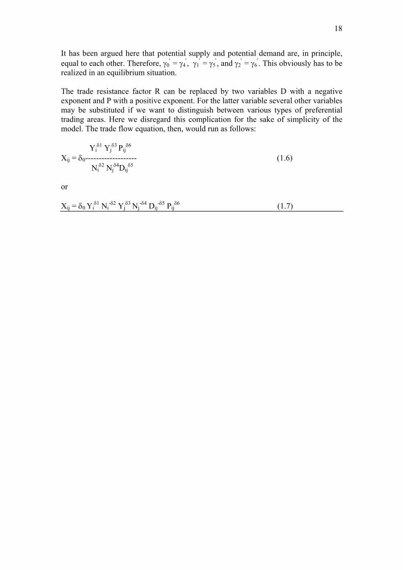
realized in an equilibrium situation. The trade resistance factor R can be replaced by two variables D with a negative exponent and P with a positive exponent. For the latter variable several other variables may be substituted if we want to distinguish between various types of preferential trading areas. Here we disregard this complication for the sake of simplicity of the model. The trade flow equation, then, would run as follows: Yi

δ1 Yjδ3 Pij

δ6

Xij = δ0------------------- (1.6) Ni

δ2 Njδ4Dij

δ5

or Xij = δ0 Yi

δ1 Ni-δ2 Yj

δ3 Nj-δ4 Dij

-δ5 Pijδ6 (1.7)

19

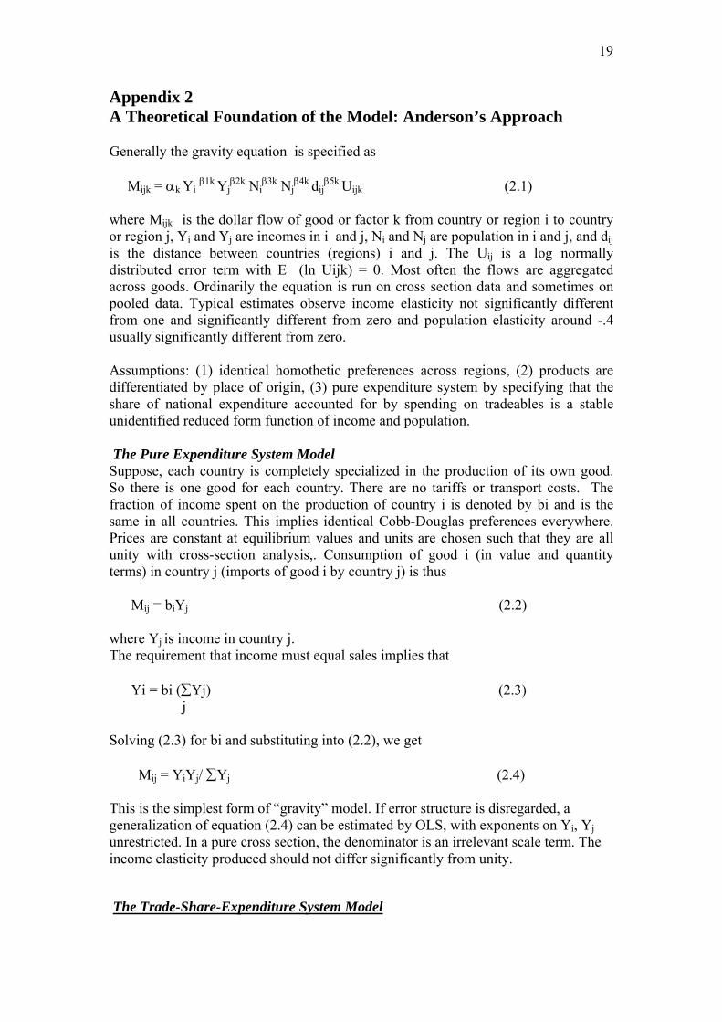
Appendix 2 A Theoretical Foundation of the Model: Anderson’s Approach Generally the gravity equation is specified as Mijk = αk Yi β1k

Yjβ2k Ni

β3k Njβ4k dij

β5k Uijk (2.1) where Mijk is the dollar flow of good or factor k from country or region i to country or region j, Yi and Yj are incomes in i and j, Ni and Nj are population in i and j, and dij is the distance between countries (regions) i and j. The Uij is a log normally distributed error term with E (ln Uijk) = 0. Most often the flows are aggregated across goods. Ordinarily the equation is run on cross section data and sometimes on pooled data. Typical estimates observe income elasticity not significantly different from one and significantly different from zero and population elasticity around -.4 usually significantly different from zero. Assumptions: (1) identical homothetic preferences across regions, (2) products are differentiated by place of origin, (3) pure expenditure system by specifying that the share of national expenditure accounted for by spending on tradeables is a stable unidentified reduced form function of income and population. The Pure Expenditure System Model Suppose, each country is completely specialized in the production of its own good. So there is one good for each country. There are no tariffs or transport costs. The fraction of income spent on the production of country i is denoted by bi and is the same in all countries. This implies identical Cobb-Douglas preferences everywhere. Prices are constant at equilibrium values and units are chosen such that they are all unity with cross-section analysis,. Consumption of good i (in value and quantity terms) in country j (imports of good i by country j) is thus Mij = biYj (2.2) where Yj is income in country j. The requirement that income must equal sales implies that Yi = bi (∑Yj) (2.3)

j Solving (2.3) for bi and substituting into (2.2), we get Mij = YiYj/ ∑Yj (2.4)

This is the simplest form of “gravity” model. If error structure is disregarded, a generalization of equation (2.4) can be estimated by OLS, with exponents on Yi, Yj unrestricted. In a pure cross section, the denominator is an irrelevant scale term. The income elasticity produced should not differ significantly from unity.

The Trade-Share-Expenditure System Model

20

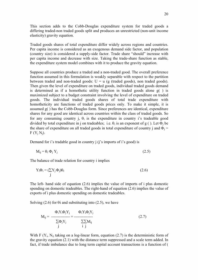
This section adds to the Cobb-Douglas expenditure system for traded goods a differing traded-non traded goods split and produces an unrestricted (non-unit income elasticity) gravity equation. Traded goods shares of total expenditure differ widely across regions and countries. Per capita income is considered as an exogenous demand side factor, and population (country size) is considered a supply-side factor. Trade share “should” increase with per capita income and decrease with size. Taking the trade-share function as stable, the expenditure system model combines with it to produce the gravity equation. Suppose all countries produce a traded and a non-traded good. The overall preference function assumed in this formulation is weakly separable with respect to the partition between traded and non-traded goods: U = u (g (traded goods), non traded goods). Then given the level of expenditure on traded goods, individual traded goods demand is determined as if a homothetic utility function in traded goods alone g( ) is maximized subject to a budget constraint involving the level of expenditure on traded goods. The individual traded goods shares of total trade expenditure with homotheticity are functions of traded goods prices only. To make it simple, it is assumed g( ) has the Cobb-Douglas form. Since preferences are identical, expenditure shares for any good are identical across countries within the class of traded goods. So for any consuming country j, θi is the expenditure in country i’s tradeable good divided by total expenditure in j on tradeables; i.e. θi is an exponent of g ( ). Let Φj be the share of expenditure on all traded goods in total expenditure of country j and Φj = F (Yj Nj).

Demand for i’s tradable good in country j (j’s imports of i’s good) is Mij = θi Φj Yj (2.5) The balance of trade relation for country i implies YiΦi = (∑Yj Φj)θI (2.6) j The left- hand side of equation (2.6) implies the value of imports of i plus domestic spending on domestic tradeables. The right-hand of equation (2.6) implies the value of exports of i plus domestic spending on domestic tradeables. Solving (2.6) for θi and substituting into (2.5), we have ΦiYiΦjYj ΦiYiΦjYj Mij = -------------- = -------------- (2.7) ∑ΦjYj ∑∑Mij j i j With F (Yi, Ni) taking on a log-linear form, equation (2.7) is the deterministic form of the gravity equation (2.1) with the distance term suppressed and a scale term added. In fact, if trade imbalance due to long term capital account transactions is a function of (

21

Yi,Ni), we may write the basic balance YiΦimi = (∑YjΦj)θi, with mi = m (Yi, Ni), and substitute into (2.6) and (2.7). j This yields miΦiYiΦjYj Mij = --------------------- (2.8) ∑∑Mij

i j With log-linear forms for m and F, (2.8) is again essentially the deterministic gravity equation.

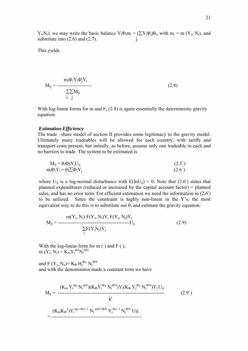
Estimation Efficiency The trade –share model of section II provides some legitimacy to the gravity model. Ultimately many tradeables will be allowed for each country, with tariffs and transport costs present, but initially, as before, assume only one tradeable in each and no barriers to trade. The system to be estimated is Mij = θiΦjYjUij (2.5´) miΦiYi = θi∑ΦjYj (2.6´)

where Uij is a log-normal disturbance with E(lnUij) = 0. Note that (2.6′) states that planned expenditures (reduced or increased by the capital account factor) = planned sales, and has no error term. For efficient estimation we need the information in (2.6′) to be utilized. Since the constraint is highly non-linear in the Y’s, the most equivalent way to do this is to substitute out θi and estimate the gravity equation: m(Yi, Ni) F(Yi, Ni)Yi F(Yj, Nj)Yj Mij = -------------------------------------------Uij (2.9) ∑F(YjNj)Yj j

With the log-linear form for m ( ) and F ( ), m (Yi, Ni) = KmYi

myNimN

and F (Yj, Nn)= KΦ Hj

Φy NjΦN

and with the denominator made a constant term we have (Km Yi

my NimN)(KΦYi

Φy NiΦN)Yi(KΦ Yj

Φy NjΦN)Yj Uij

Mij = ---------------------------------------------------------------- (2.9´) k′ (KmKΦ

2)Yimy+Φy+1 Ni

mN+ΦN YjΦy+1 Nj

ΦN Uij = ------------------------------------------------------

22

K′ This is the aggregate form of equation (2.1) with the distance term omitted. Ordinarily it can be fitted on a subset of countries in the world. Exports to the rest of the world are exogenous and imports from it are excluded from the fitting. If this is done, the denominator is still the sum of world trade expenditures, and (2.6′) implies that (2.9) and (2.9′) assume that θi is the same in the excluded countries as in the included countries. Finally, form the set of estimated values for traded-goods expenditures: Λ Λ Λ Λ

ΦjYj = KΦYjΦy+1 Nj

ΦN (2.10) ^

The individual traded-goods shares θi can be estimated using the instruments ΦjYj (which are asymptotically uncorrelated with Uij): Λ

Mij = θiΦjYjUij (2.11)

which is estimated across countries for country i’s exports (including the rest of the world’s exports to included countries), with the restriction that ∑θi = 1.

23

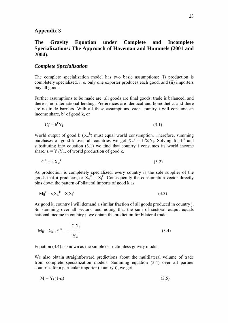
Appendix 3 The Gravity Equation under Complete and Incomplete Specializations: The Approach of Haveman and Hummels (2001 and 2004). Complete Specialization The complete specialization model has two basic assumptions: (i) production is completely specialized, i. e. only one exporter produces each good, and (ii) importers buy all goods. Further assumptions to be made are: all goods are final goods, trade is balanced, and there is no international lending. Preferences are identical and homothetic, and there are no trade barriers. With all these assumptions, each country i will consume an income share, bk of good k, or Ci

k = bkYi (3.1)

World output of good k (Xw

k) must equal world consumption. Therefore, summing purchases of good k over all countries we get Xw

k = bkΣiYi. Solving for bk and substituting into equation (3.1) we find that country i consumes its world income share, si = Yi/Yw, of world production of good k. Ci

k = siXwk (3.2)

As production is completely specialized, every country is the sole supplier of the goods that it produces, or Xw

k = Xjk

. Consequently the consumption vector directly pins down the pattern of bilateral imports of good k as Mij

k = siXwk = SiXj

k (3.3) As good k, country i will demand a similar fraction of all goods produced in country j. So summing over all sectors, and noting that the sum of sectoral output equals national income in country j, we obtain the prediction for bilateral trade: YiYj Mij = Σk siYj

k = --------- (3.4) Yw

Equation (3.4) is known as the simple or frictionless gravity model. We also obtain straightforward predictions about the multilateral volume of trade from complete specialization models. Summing equation (3.4) over all partner countries for a particular importer (country i), we get Mi = Yi (1-si) (3.5)

24

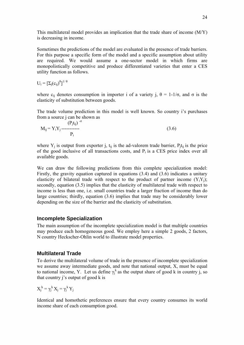
This multilateral model provides an implication that the trade share of income (M/Y) is decreasing in income. Sometimes the predictions of the model are evaluated in the presence of trade barriers. For this purpose a specific form of the model and a specific assumption about utility are required. We would assume a one-sector model in which firms are monopolistically competitive and produce differentiated varieties that enter a CES utility function as follows. Ui = [Σj(cij)θ]1/ θ

where cij denotes consumption in importer i of a variety j, θ = 1-1/σ, and σ is the elasticity of substitution between goods. The trade volume prediction in this model is well known. So country i’s purchases from a source j can be shown as (Pjtij) -σ Mij = YiYj ----------- (3.6) Pi

where Yj is output from exporter j, tij is the ad-valorem trade barrier, Pjtij is the price of the good inclusive of all transactions costs, and Pi is a CES price index over all available goods. We can draw the following predictions from this complete specialization model: Firstly, the gravity equation captured in equations (3.4) and (3.6) indicates a unitary elasticity of bilateral trade with respect to the product of partner income (YiYj); secondly, equation (3.5) implies that the elasticity of multilateral trade with respect to income is less than one, i.e. small countries trade a larger fraction of income than do large countries; thirdly, equation (3.6) implies that trade may be considerably lower depending on the size of the barrier and the elasticity of substitution.

Incomplete Specialization The main assumption of the incomplete specialization model is that multiple countries may produce each homogeneous good. We employ here a simple 2 goods, 2 factors, N country Heckscher-Ohlin world to illustrate model properties.

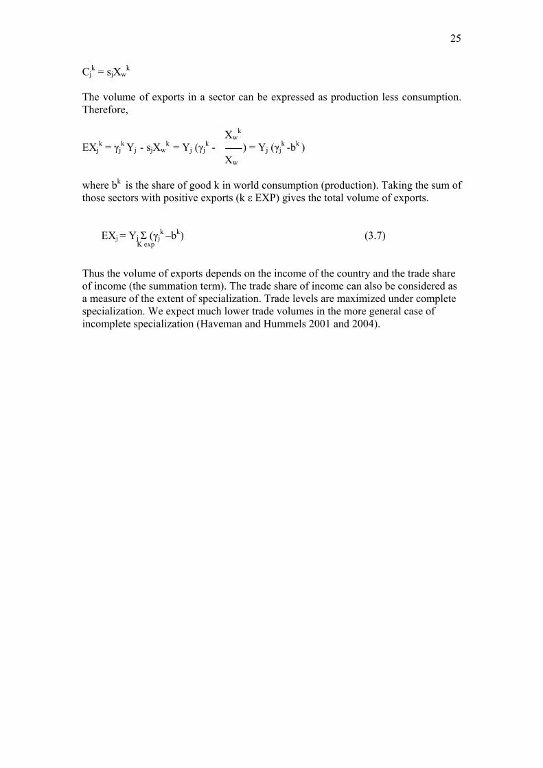
Multilateral Trade To derive the multilateral volume of trade in the presence of incomplete specialization we assume away intermediate goods, and note that national output, X, must be equal to national income, Y. Let us define γj

k as the output share of good k in country j, so that country j’s output of good k is Xj

k = γjk Xj = γj

k Yj

Identical and homothetic preferences ensure that every country consumes its world income share of each consumption good.

25

Cjk = sjXw

k

The volume of exports in a sector can be expressed as production less consumption. Therefore, Xw

k

EXjk = γj

k Yj - sjXwk = Yj (γj

k - ) = Yj (γjk -bk )

Xw

where bk is the share of good k in world consumption (production). Taking the sum of those sectors with positive exports (k ε EXP) gives the total volume of exports. EXj = Yj Σ (γj

k –bk) (3.7) K exp

Thus the volume of exports depends on the income of the country and the trade share of income (the summation term). The trade share of income can also be considered as a measure of the extent of specialization. Trade levels are maximized under complete specialization. We expect much lower trade volumes in the more general case of incomplete specialization (Haveman and Hummels 2001 and 2004).

26

Appendix 4

Results of the Extreme Bounds Sensitivity Analysis

Export Model ============================================================= Variable of Coefficient t-statistic R2 Control Variable(s) Results Interest log(To.Impj) High 1.0373 10.72 0.43 log(Exc.Rate)ij Base 1.0896 11.32 0.42 robust Low 0.8237 8.28 0.46 (TR/GDP)i

log(Exc.Rate)ij High 0.1031 4.37 0.43 (TR/GDP)i Base 0.1215 4.84 0.35 robust Low 0.0813 3.42 0.43 log(To.Impj) (TR/GDP)i High 4.3591 10.51 0.42 log(Exc.Rate)ij Base 4.4940 10.74 0.41 robust Low 3.2310 7.52 0.46 log(To.Impj) log(CPIi) High 1.2591 0.50 0.47 log(Exc.Rate)ij., log(CPIj) Base 1.5474 0.61 0.44 fragile Low 0.2368 0.09 0.46 log(To.Impj), (TR/GDP)I

log(CPIj) High 0.1253 0.53 0.48 log(Exc.Rate)ij, (TR/GDP)i Base 0.1102 0.45 0.44 fragile Low 0.0212 0.09 0.46 log(To.Impj), log(CPIi)

27

Table 1 Hetero Corrected Fixed Effects Models with Group Dummy Variables

Variables Export Model (TR/GDP)i 2.27 (6.65) Log (Exc.Rate)ij 0.34 (6.78) Log (To.Impj) 1.01 (11.41) R2 0.79 F 88.78 [32, 752] Observations 785 t-ratios are noted in parentheses. Table 1(A) Country Specific Effects

Export Model

Estimated Fixed Effects Country Coefficient t-ratio India -3.98161 -11.35915 Nepal -3.18347 -15.06288 Pakistan -3.19659 -10.12779 Sri Lanka -3.71255 -13.46857 Indonesia -4.12012 -10.67744 Malaysia -4.88221 -14.30029 The Philippines -4.79015 -14.41902 Thailand -4.39164 -12.51778 Canada -4.80324 -12.09441 Mexico -5.92536 -16.38100 USA -4.34713 -9.60586 Belgium -4.04340 -9.75353 Denmark -4.39586 -11.72100 France -4.72039 -11.04269 Germany -4.47119 -9.70940 Greece -4.27493 -12.30002 Italy -3.44276 -7.62768 The Netherlands -4.67158 -11.39545 Portugal -4.35928 -12.29574 Spain -4.37484 -10.94045 Sweden -4.93010 -13.01129 United kingdom -4.51311 -10.73042 Egypt -4.07449 -12.66137 Iran -3.15882 -8.69149 Syrian A.R. -3.39184 -11.65424 Australia -4.39423 -12.12841 New Zealand -4.78578 -14.75875 Japan -4.02982 -8.92404 China -4.60817 -12.35827 Hong Kong -4.54601 -12.02473

28

Table 2 Cross-Section Results of the Distance and Dummy Variables. Dependent Variable is Country Specific Effect

Variables Export Model Distance -0.44 (-0.80) ijBorder -0.62 (-1.25) J-SAARC -1.98 (-1.14) J-ASEAN -3.05 (-1.62) J-EEC -2.68 (-1.26) J-NAFTA -3.21 (-1.42) J-Middle East -1.92 (-0.94)

J- others -2.84 (-1.39) R2 0.62 F 5.09[7,22] Observations 30 t-ratios are shown in the parentheses. Table 3 Multicollinearity Test

Export Model

Original R2 = 0.44 (from OLS) When Log(ERij)is the dependent Variable,R2=0.01 When Log(TIj)is the dependent Variable,R2=0.07 When (Trade/GDP)i is the dependent Variable,R2=0.07

IMPLICATIONS: Above model is free from the multicollinearity problem. Table 4 Model Selection Test- Fixed vs Random Effect Models Export Model +-----------------------------------------------------------------------+ | Least Squares with Group Dummy Variables | | Ordinary least squares regression Weighting variable = none | | Dep. var. = Log (Exp ) Mean= .9540221643 , S.D.= .8153025069 | i

| Model size: Observations = 785, Parameters = 33, Deg.Fr.= 752 | | Residuals: Sum of squares= 109.0757636 , Std.Dev.= .38085 | | Fit: R-squared= .790697, Adjusted R-squared = .78179 | | Model test: F[ 32, 752] = 88.78, Prob value = .00000 | | Diagnostic: Log-L = -339.2127, Restricted(b=0) Log-L = -953.0725 | | LogAmemiyaPrCrt.= -1.890, Akaike Info. Crt.= .948 | | Estd. Autocorrelation of e(i,t) .484127 | +-----------------------------------------------------------------------+ +---------+--------------+----------------+--------+---------+----------+ |Variable | Coefficient | Standard Error |b/St.Er.|P[|Z|>z] | Mean of X| +---------+--------------+----------------+--------+---------+----------+ log(ERijLog(TI

) .3382378886 .53452284E-01 6.328 .0000 .33723167 j) 1.010957387 .88021420E-01 11.485 .0000 4.5868303

(TR/Y)i 2.267862566 .37026738 6.125 .0000 .21044804 (Note: E+nn or E-nn means multiply by 10 to + or -nn power.)

29

Note: Country specific effects are not shown due to space consideration. +--------------------------------------------------+ | Random Effects Model: v(i,t) = e(i,t) + u(i) | | Estimates: Var[e] = .145048D+00 | | Var[u] = .225598D+00 | | Corr[v(i,t),v(i,s)] = .608662 | | Lagrange Multiplier Test vs. Model (3) = 3494.80 | | ( 1 df, prob value = .000000) | | (High values of LM favor FEM/REM over CR model.) | | Fixed vs. Random Effects (Hausman) = 14.42 | | ( 3 df, prob value = .002381) | | (High (low) values of H favor FEM (REM).) | | Reestimated using GLS coefficients: | | Estimates: Var[e] = .145684D+00 | | Var[u] = .336853D+00 | | Sum of Squares .351580D+03 | +--------------------------------------------------+ +---------+--------------+----------------+--------+---------+----------+ |Variable | Coefficient | Standard Error |b/St.Er.|P[|Z|>z] | Mean of X| +---------+--------------+----------------+--------+---------+----------+ log(ERij) .2690241714 .46589817E-01 5.774 .0000 .33723167 Log(TIj) .9240199227 .74454770E-01 12.410 .0000 4.5868303 (TR/Y) 2.578612997 .34193336 7.541 .0000 .21044804 i

Constant -3.922643965 .30927545 -12.683 .0000 (Note: E+nn or E-nn means multiply by 10 to + or -nn power.)

Table 5 Autocorrelated Error Structured Fixed Effect Model Variables Export Model (TR/GDP)i 1.85 (4.07) Log (Exc.Rate)ij 0.31 (3.63) Log (To.Impj) 1.02 (7.90) Log ( PCGDPDij) Log (Infli) Log (Inflj) R2 0.57 F 30.45 [32, 722] Observations 755 t-ratios are noted in parentheses. Note: Country specific effects are not shown because of space consideration.

30

Table 6 Descriptive Statistics

Descriptive Statistics of the Export Model Series Observation Mean Standard Deviation Minimum Maximum ----------------------------------------------------------------------------------------------------------------------- log (BD's Exp.) 785 0.954022164 0.815302507 -1 3.149527 log (dist) 785 3.688857745 0.322530148 2.826075 4.179063 Log(Exc.Rate) 785 0.337231669 0.968771228 -2.32932 2.982994 Log(T.Impj) 785 4.58683031 0.670836758 2.264374 6.095859 (Trade/GDP)i 785 0.21044804 0.054185706 0.090705 0.318445 D1(j-SAARC) 785 0.142675159 0.349964251 0 1 D2(j-ASEAN) 785 0.142675159 0.349964251 0 1 D3(j-EEC) 785 0.347770701 0.476566427 0 1 D4(j-NAFTA) 785 0.107006369 0.309318427 0 1 D5(j-M.East) 785 0.100636943 0.30103919 0 1 D6(j- 0ther) 785 0.159235669 0.366128987 0 1 D7(border) 785 0.03566879 0.18558125 0 1 Table 7 Correlation Matrices

Correlation Matrix of the Export Model Log(BD's Exp.) Log(Exc.Rate) Log (T.Impj) (Trade/GDP)i log (BD's Exp.) 1 Log(Exc.Rate) 0.13346523 1 Log(T.Impj) 0.622063324 0.113451808 1 (Trade/GDP)i 0.384046956 0.057624011 0.25481981 1

Corrrelation Matrix of Distance and Dummies for the Export Model Ind.effect Ldist D1-bor D2-j SA D3-j ASE D4-jEE D5-j NAF D6-J-M.E D7-j other Ind.effect 1 Ldist -0.49518 1 D1-border 0.093312 -0.32012 1 D2-J SAARC 0.502597 -0.67617 0.473432 1 D3-J ASEAN -0.1741 -0.34241 -0.07284 -0.15385 1 D4-J EEC -0.12513 0.432291 -0.14129 -0.29844 -0.29844 1 D5-J NAFTA -0.41317 0.444371 -0.0619 -0.13074 -0.13074 -0.25363 1 D6-J-Meast 0.415028 -0.00735 -0.0619 -0.13074 -0.13074 -0.25363 -0.11111 1 D7-other -0.13933 0.018322 -0.08305 -0.17541 -0.17541 -0.34028 -0.14907 -0.14907 1 Note: D1= border, D2= j-SAARC, D3= j-ASEAN, D4= j-EEC, D5= j-NAFTA, D6= j-M. East, D7= j- Other.

31

Table 8 The Export Model with the Gravity Variables Only Variables Export Model GDPi -0.48 (-.08) GDPj 0.71 (17.48)* Distance -0.73 (-8.36)* R2 0.31 F 175.25[2, 782] Observation 785 t-ratios are in parentheses. * denotes significant at 1% level.

Table 9 Fixed Effects Models with Multilateral Resistance Variables

Variables Export Model (TR/GDP)i -0.49(-0.65) Log (Exc.Rate)ij 0.46 (2.79) Log (To.Impj) 0.16 (0.76) Log(CPIi) 1.53(2.90) Log(CPIj) 0.46 (1.90) R2 0.86 F 65.77[34, 373] Observations 408 t-ratios are noted in parentheses.

Table 10 Cross-Section Results of the Multilateral Resistance and Dummy Variables. Dependent Variable is Country Specific Effect

Variables Export Model Remi 0.42 (0.18) Remj 0.42 (0.18) ijBorder 1.13 (0.77) J-SAARC -0.27(-0.19) J-ASEAN 0.76 (0.68) J-EEC -0.71 (-0.49) J-NAFTA 1.03(0.68) J- others -0.89 (-0.39)

R2 0.12 F 0.34[8,21] Observations 30 t-ratios are shown in the parentheses.

32

33

REFERENCES Anderson, J.E. (1979) A Theoretical Foundation for the Gravity Equation, The American Economic Review, 69, 106-16.

Anderson, J.E. and Wincoop E. V. (2003) Gravity with Gravitas: A Solution to the Border Puzzle, The American Economic Review, 93 (1), 170-92, Nashville. Baier, S. L and Bergstrand, J. H. (2003) Endogenous Free Trade Agreements and the Gravity Equation, Working Paper, Downloaded. Bergstrand J.H. (1989) The Generalised Gravity Equation, Monopolistic Competition, and the Factor Proportion Theory in International Trade, Review of Economics and Statistics, 143-53.

Bergstrand, J.H., (1985) The Gravity Equation in International Trade: Some Microeconomic Foundations and Empirical Evidence, The Review of Economics and Statistics, 67, 474-81. Harvard University Press. Carrillo, C. and Li, C. A. (2002) Trade Blocks and the Gravity Model: Evidence from Latin American Countries, Working Paper (downloaded), Department of Economics, University of Essex, UK.

Christie, E. (2002) Potential Trade in Southeast Europe: A Gravity Model Approach, Working Paper, The Vienna Institute for International Economic Studies-WIIW downloaded on 14 March 2002.

Davis, D. and Weinstein, D. (1996) Does Economic Geography Matter for International Specialisation? NBER Working Paper, No. 5706, Cambridge Mass: National Bureau of Economic Research.

Deardorff, A.V. (1984) Testing Trade Theories and Predicting Trade Flows, Handbook of International Economics 1, Amsterdam, North-Holland. Deardorff, A., (1998) Determinants of Bilateral Trade: Does Gravity Work in a Classical World? In The Regionalization of the World Economy (Ed.) J. Frankel, Chicago: University of Chicago Press. Dreze, J. (1961) Leo Exportation Intra-CEE en 1958 et al Position Belge, Recherches Economiques de Louvain (louvin), 27, 7171-738. Eaton, J. and Kortum, S. (1997) Technology and Bilateral Trade. NBER Working Paper, No. 6253, Cambridge, MA: National Bureau of Economic Research.

Evenett, S.J. and Keller, W. (1998) On the Theories Explaining the Success of the Gravity Equation, NBER Working Paper, No. 6529, Cambridge, MA: National Bureau of Economic Research.

34

Feenstra, R. (2003) Advanced International Trade: Theory and Evidence. Chapter 5, Princeton University Press. Frankel, J.A. (1997) Regional Trading Blocs in the World Economic System, Institute for International Economics, Washington, D.C.

Haveman, J. and Hummels, D. (2001) Alternative Hypotheses and the Volume of Trade: The Gravity Equation and the Extent of Specialization, Working Paper, Federal Trade Commission (Downloaded on 3 August ‘04 from Google).

Hassan, M.K. (2000) Trade Relations with SAARC Countries and Trade Policies of Bangladesh, Journal of Economic Cooperation Among Islamic Countries, 21(3), 99-151. Hassan, M.K. (2001) Is SAARC a Viable Economic Block? Evidence from Gravity Model, Journal of Asian Economics, 12, 263-290.

Hassan, M.K. (2002) Trade with India and Trade Policies of Bangladesh, in Towards Greater Sub-regional Economic Cooperation (Eds.) F. E. Cookson and A.K.M.S. Alam, chapter 10, 349-401. Helpman, E and Krugman, P. (1985) Market Structure and Foreign Trade, Cambridge, MA: MIT Press.

Helpman, E., (1981) International Trade in the Presence of Product Differentiation, Economies of Scale and Monopolistic Competition: A Chamberlin Heckscherlin-Ohlin Approach, Journal of International Economics, 11, 305-40.

Helpman, E. (1984) Increasing Returns, Imperfect Markets, Trade Theory, in Handbook of International Economics 1 (Eds) W. J. Ronald and B. K. Peter, Amsterdam, North-Holland.

Helpman, E. (1987) Imperfect Competition and International Trade: Evidence from fourteen Industrial Countries, Journal of Japanese and International Economics, 1, 62-81. Helpman, E. (1989) Monopolistic Competition in Trade Theory, Frank Graham Memorial Lecture, 1989 special paper 16, International Finance Section, Princeton University, Princeton, N.J.

Helpman, E. and Krugman P.R. (1985) Market Structure and Foreign Trade: Increasing Return, Imperfect Competition, and International Economy, Cambridge, USA. Helpman, E. and Krugman, P.R. (1989) Trade Policy and Market Structure, Cambridge Mass: MIT Press.

35

IMF. (various years) Direction of Trade Statistics Yearbook, International Monetary Fund, Washington, D.C.

IMF. (various years) International Financial Statistics (IFS) CD-ROM. International Monetary Fund, Washington, D.C. Jakab,Z.M. et. al (2001) How Far Has Trade Integration Advanced?: An Analysis of the Actual and Potential Trade of Three Central and Eastern European Countries, Journal of Comparative Economics, 29, 276-92.

Karemera, D. et al (1999) A Gravity Model Analysis of the Benefits of Economic Integration in the Pacific Rim, Journal of Economic Integration, 14 (3), 347-67, September. Koo, W.W. and Karemera, D. (1991) Determinants of World Wheat Trade Flows and Policy Analysis, Canadian Journal of Agricultural Economics, 39, 439-55.

Krugman, P. (1979) Increasing Returns, Monopolistic Competition, and International Trade, Journal of International Economics, 9, 469-79.

Lancaster, K. (1980) Intra-Industry Trade Under Perfect Monopolistic Competition, Journal of International Economics, 10, 151-75. Le, et.al (1996) Vietnam’s Foreign Trade in the Context of ASEAN and Asia-Pacific Region: A Gravity Approach, ASEAN Economic Bulletin, 13 (2). Levine, R. and Renelt, D. 1992. ‘A Sensitivity Analysis of Cross-Country Growth Regressions’, The American Economic Review, Vol.82, No. 4: 942-963. Linder, S. B. (1961) An Essay on Trade and Transformation. New York: John Wiley and Sons.

Linneman, H. (1966) An Econometric Study of International Trade Flows. North Holland, Amsterdam. Mathur, S.K. (1999) Pattern of International Trade, New Trade Theories and Evidence from Gravity Equation Analysis, The Indian Economic Journal, 47(4), 68-88. Mátyás, L. (1997) Proper Econometric Specification of the Gravity Model, The World Economy, 20 (3).

Mátyás, L. et. al. (2000) Modelling Export Activity of Eleven APEC Countries, Melbourne Institute Working Paper No. 5/00, Melbourne Institute of Applied Economic and Social Research, The University of Melbourne, Australia.

36

McCallum, J. (1995) National Borders Matter: Canada-U.S. Regional Trade Patterns, The American Economic Review, 85 (3), 615-623.

Oguledo, V.I. and Macphee, C.R. (1994) Gravity Models: A Reformulation and an Application to Discriminatory Trade Arrangements, Applied Economics, 26, 107-20. Paas, T. (2000) Gravity Approach for Modeling Trade Flows between Estonia and the Main Trading Partners, Working Paper, No. 721, Tartu University Press, Tartu. Posner, M.V. (1961) International Trade and Technical Changes. Oxford Economic Papers, 13, 323-41.

Pöyhönen, P. (1963) Toward A General Theory of International Trade, Ekonomiska Samfundets Tidskrift, Tredje serien, Argang, 16, 69-77. Rajapakse, P and Arunatilake, N. (1997) Would a Reduction in Trade Barriers Promote Intra-SAARC Trade?: A Sri Lankan Perspective, Journal of Asian Economics, 81, 95-115. Sharma, S. C. and Chua, S.Y. (2000) ASEAN: Economic Integration and Intra-Regional Trade, Applied Economics Letters, 7(3), 165-69, (March).

Soloaga, I and Winters, L.A. (2001) How has Regionalism in the Nineties Affected Trade? North American Journal of Economics and Finance, 12, 1-29.

Thursby, J,G. and Thursby M.C. (1987) Bilateral Trade Flows, the Linder Hypothesis and Exchange Risk, Review of Economics and Statistics, 69, 488-95.

Vernon, R. (1966) International Investment and International Trade in the Product Cycle, Quarterly Journal of Economics, 80, 190-207.

World Bank (2004) World Development Indicators, CD-ROM, World Bank, Washington D.C. World Bank (2001) World Development Indicators CD-ROM, World Bank, Washington D.C. WDI. (various years) World Development Indicators, World Bank., Washington, D.C.

Yamarik, S. and Ghosh, S. 2005. ‘A Sensitivity Analysis of the Gravity Model’, The International Trade Journal, Vol. 19, No. 1, Spring 2005. Zhang, J. and Kristensen, G. (1995) A Gravity Model with Variable Coefficients: The EEC Trade with Third Countries, Geographical Analysis, 27, 307-20. ===============================================