The Challenges of Achieving Kenya’s Vision 2030:

A Macro Perspective

Hans Lofgren

and

Praveen Kumar

World Bank

Background paper for Country Economic Memorandum

Draft, August 24, 2007

2

1. INTRODUCTION AND SUMMARY

The development policies of the government of Kenya are driven by the objective of

achieving Vision 2030, under which the key objective is to accelerate GDP growth to an

annual rate of 10 percent. This is a very ambitious objective considering that, during the

last 25 years, annual real GDP growth was merely 3% (World Bank 2007).

In this paper, we explore what may be required for Kenya to achieve this objective. Our

work takes a macro perspective and is meant to complement sector- and micro-oriented

policy analysis. Methodologically, we combine simulations of alternative scenarios for

Kenya’s economy for the period 2006-2030 with a discussion of the implications of the

results for policy makers. The simulations rely on a macro-oriented Kenyan version of

MAMS (Maquette for MDG Simulations), a tool developed at the World Bank for

analysis of development strategies.

In the simulations, we investigate the potential roles of likely driving forces behind the

required growth acceleration. More specifically, we first introduce, one by one, increases

in national savings, foreign direct investment (FDI), and foreign aid. Subsequently, we

simulated the effect of combining changes in these growth determinants with increases in

TFP (total factor productivity) growth. The advantage of using a model like MAMS for

this type of analysis is that it, in a consistent and comprehensive manner, simulates the

combined impact of these changes on major economic indicators (including GDP, trade,

private and government consumption and investment, considering the presence of

constraints at the macro level (represented by fiscal, foreign exchange, and savings-

investment balances) and in factor markets and using standard assumptions about the

behavior of producers, consumers, and government.

Under the BASE scenario, which is a business-as-usual scenario that extrapolates on the

recent pick-up in economic performance, GDP and most other aggregate indicators grow

at around 5% per year, out of which 3.9% is due to increased factor employment and

1.1% due to increased TFP. There are no major changes in the GDP shares of the national

3

account aggregates or of major spending and receipt items in the government budget and

the balance of payments.

High national savings rates are needed to sustain rapid GDP growth and high investment

rates. The scenario BASE+GNS is identical to BASE except for a 50% increase in the

GNS rate during 2007-2017, from 15.7% to 23.5%, via an increase in private savings

rates. After 2017, the GNS rate stays at 23.5%. For the period 2007-2030, this change

leads to a strong increase in private investment, increasing growth in GDP by 1.6%, with

a particularly strong increase for private investment. Due to the savings increase, private

consumption growth initially slows down compared to other scenarios.

FDI may increase (and decrease) more rapidly than more slow-moving domestic

financing sources and may lead to more rapid technological progress than investment by

domestic firms. Under the scenario BASE+FDI, FDI gradually increases from a very low

level in 2006 to 4% of GDP in 2017, a GDP share that is retained, with a slight decline,

up to 2030. The scenario does not consider possible direct technological gains from FDI.

The simulated effects are quite similar to those of the simulated GNS increase (but

roughly half as large, given the smaller magnitude of the shock): a strong increase in

private investment growth is coupled with a smaller growth increase for GDP and other

national account aggregates.1 Initially, private consumption and welfare fares better since

there is no need to switch private income to savings. However, over time, growth in profit

repatriation forces more export growth while reducing import growth (given balance of

payments constraints a lower trade deficit is required), dampening the long-run positive

impact on absorption (private and government consumption and investment) and welfare.

Foreign aid relaxes the budget constraint of the government, permitting increases in

domestic consumption and investment. Under the scenario BASE+AID, aid (the part

represented by current transfers from the rest of the world to the government) is increased

1 The relative magnitudes of the shocks reflect what was considered plausible. Cross-country data indicate that the bulk of investment is typically financed from domestic sources. For high-investment countries, it is rare that foreign savings (out of which FDI is a part) finances more then 20% of investment (Rodrik 2000, p. 481).

4

gradually from a low level to around 4% of GDP in 2017, i.e., a magnitude that is similar

to the FDI level under BASE+FDI. It is kept close to this share up to 2030. The extra aid

is used to reduce taxes. Government spending will increase in so far as GDP grows more

rapidly.2 Households allocate their additional incomes to savings that feed into domestic

private investment. The growth effects are very similar to those of BASE+FDI but the

welfare effects are more positive since grant aid does not lead to any resource outflow

corresponding to profit repatriation. It also avoids the initial dampening of private

consumption growth that is required under BASE+GNS.

The preceding scenarios have relaxed domestic resource constraints, permitting more

savings, investments, and growth. However, they have only had smaller, indirect effects

on TFP growth, the acceleration of which has to be at the core of Kenya’s Vision 2030

strategy. More rapid TFP growth would be likely in the context of rapid increases in

investment (including FDI) and private savings, supported by increased aid. Hence, the

scenario V30-GRADUAL combines the changes in the preceding scenarios (in GNS,

FDI, and aid) with an increase in TFP growth sufficient to gradually raise GDP growth to

10% by 2017, a rate that is maintained up to 2030. The results indicate that this growth

acceleration requires annual TFP growth at 2.6%, a rate that is far in excess of Kenya’s

recent record (but actually slightly below the rate achieved during the first 13 years of

independence) (Ndulu 2007, p. 53).3 Under this scenario, the growth rates for the full

period 2006-2030 are around 9% for GDP, 12% for private investment, and 8-11% for

other national account aggregates. In 2030, private consumption per capita is 270%

higher than in 2006, i.e. not far from quadrupled.

The final scenario, V30-FAST is similar to V30-GRADUAL except for that the changes

now are introduced more quickly, during the period 2007-2013, after which GDP growth

stays at 10%. Annual growth in TFP and most national account aggregates increase by an

2 The underlying assumption is that decisions about private vs. government shares in the economy do not depend on the size of foreign aid. However, if GDP growth increases or decreases, then government consumption and investment will also increase/decrease sufficiently to maintain unchanged GDP shares. 3 For the full period 1960-2004, Kenya’s TFP growth was 0.0%; its annual GDP growth of 4% was due to a combination of capital growth (2.1%) and labor growth (1.9%) (Tahari et al. 2004, p. 17).

5

additional 0.2-0.5% (compared to V30-GRAUAL). In the final year, private per-capita

consumption is 310% above the level in 2006.

In terms of policy, what can be done to bring about such scenarios or, more broadly, to

drastically accelerate growth in Kenya? Accumulated evidence suggests that the factors

that may initiate the strived-for acceleration are increases in investment, including FDI

accompanied by technological improvements. In the short to medium run, it is possible to

improve governance and infrastructure, giving a needed boost to the investment climate

and raising TFP (especially via reduced transactions costs). In the long run, human

capital improvements are an essential ingredient of a good investment climate supportive

of rapid TFP growth. Increases in private savings rates are more likely to follow than lead

given that they respond to income growth and changes in per-capita income levels and

dependency ratios that only change more slowly. Further improvements in Kenya’s

already highly developed financial sector may provide better incentives to savers and

more efficiently channel their funds to private investors. Kenya can do less to influence

aid inflows, esp. in grant form. However, aid can play a critical role, especially in the

beginning of the growth acceleration. Improvements in governance and the investment

climate, combined with initial signs of success, should convince donors that additional

aid would be put to good use with long-lasting positive effects on welfare and poverty

reduction.

In outline, the rest of this paper proceeds as follows: Section 2 provides background on

the model that is used, with an emphasis on the treatment of growth. Section 3 describes

the simulations and analyzes the results. References, Tables and Figures are found at the

end of the paper.4

2. MODEL STRUCTURE AND GROWTH ASSUMPTIONS

4 The database underlying the model will be presented in more details in a separate document. In this paper, reference is made to data that is important for the discussion of specific points.

6

MAMS is an economywide simulation model designed to analyze development strategies

in different countries. In this paper, we are using a version of MAMS that is oriented

toward macroeconomic analysis, suppressing parts of the model that are not relevant for

this purpose and focusing our discussion on macroeconomic results.

The model is a dynamic-recursive, open-economy computable general equilibrium (CGE)

model. Like other models in this class, it provides a comprehensive and consistent picture

of the economy. It covers both private and government sectors.5 Production factors are

disaggregated into agricultural land, three types of labor (distinguished by level of

education), private capital, and different types of government capital (distinguished by

government function). All production activities use labor and intermediate inputs. The

private sector also uses land and private capital whereas government activities use

government capital.

The government consumes, invests, and pays interest on its domestic and foreign debts.

The government finances these outlays with domestic taxes, domestic borrowing, and

current and capital transfers from the rest of the world, and foreign borrowing.6 Foreign

aid may be defined as the sum of these transfers and foreign borrowing.7 The rules

determining government spending and receipts are presented in the simulation section.

Growth in the stock of government infrastructure capital contributes to overall growth by

adding to the productivity of other production activities.

Apart from the government, the institutions of the economy include households, an NGO,

and the rest of the world. Households receive their incomes from factor incomes and

transfers (from the government or the rest of the world). For factors, the income shares of

households reflect the shares they hold of the total endowments. For private capital, this

share depends on each household’s base-year share, depreciation, and new investments.

Their incomes may be used for consumption, taxes, savings and (net) transfers: after

5 The government sectors are disaggregated into education (split into three cycles), health, water-sanitation, other infrastructure, and other government. 6 Both domestic and foreign borrowing (and the corresponding debt stocks) are net terms. Increases (decreases) in foreign reserves are viewed as negative (positive) foreign borrowing 7 No distinction is made between project and program aid.

7

paying direct taxes, a fixed share of the remaining income is typically saved. After

deducting transfers, what remains is spent on consumption. The NGO receives all of its

income as transfers from the rest of the world and uses it to demand health and education

services. For each household and the NGO, receipts and payments are always equal.

The rest of the world supplies Kenya with foreign exchange by buying Kenya’s exports;

lending; providing transfers, grants and factor incomes; and investing directly in Kenya’s

economy. Kenya uses its foreign exchange to make payments related to imports, interest,

and incomes from private capital. The share of the rest of the world in total private capital

incomes depends on its share in the initial stock, depreciation and new FDI.

The model is based on standard assumptions about economic behavior. Households

allocate their consumption across different commodities on the basis of utility

maximization. Producers make profit-maximizing decisions in competitive markets. They

allocate their outputs between exports and domestic sales on the basis of relative prices.

Similarly, domestic demanders respond to relative price changes when they split their

demands between imports and domestic output.

As part of consistency requirements, the model requires that, for each institution and

production activity, total receipts be equal to total payments (including savings, if

relevant). It also requires that a set of “system constraints” be satisfied. These cover

markets for factors and commodities and macro balances.

In the markets for factors and commodities, the system constraints impose equality

between the quantities supplied and demanded. The same holds for the receipts of the

suppliers and the payments of the demanders. Markets clear via adjustments in prices (or

wages).8 In international markets, Kenya is treated is a price-taker: its decisions regarding

8 In any time period, the producers face an upward-sloping supply of labor for employment; the higher the employment rate (lower the unemployment rate), the higher the wage. The elasticity of the wage with respect to the employment rate is set at 1.5. The supply curve becomes vertical when the employment rate has reached 95% (5% unemployment rate), at which point labor is considered as “fully” employed. At full employment, the market clears via wage variations.

8

export and import quantities have no influence on the international price at which the

transactions take place.

At the macro level, the system constraints consist of balances for the government, the rest

of the world (foreign exchange), and savings-investments. In each of these three

balances, the receipts and the payments (with savings included among the payments of

government and rest of world) must be of equal value. For each balance, some

mechanism assures that receipts and payments are equal. For the government, the budget

is kept in balance via upward or downward scaling of all domestic tax rates (both direct

and indirect). 9 In The account of the rest of the world (the balance of payments) is kept in

balance via variations in the real exchange rate (which influence export and import

quantities by changing relative prices). For the savings-investment balance, the clearing

variable is invariably private investment, i.e., private investment is “savings-driven,”

determined by available funding, defined as the difference between private savings and

government borrowing, supplemented by foreign direct investment (FDI)

The model is described as “dynamic-recursive”: this means that it may be solved one year

at a time with exogenous or endogenous updating of different stocks (factors, population,

and debts). It also means that agents do not make their decisions on the basis of perfect

knowledge about the future but rather draw on current and past events.

The model treats GDP growth in a standard manner: it is determined by growth in factor

employment and in factor productivity (or efficiency). The latter may be summarized by

a measure of total factor productivity (TFP). Given the focus of the paper on growth

issues, we will here explain this in some detail.

For land and labor factors, stock growth is exogenous (determined outside the model).

Among the labor types, growth is more rapid the more educated the labor type. For land,

9 Domestic taxes were selected since (i) together they represent a substantial share of GDP; (ii) they are under government control; and (ii) changes in the GDP shares would not lead to unsustainable stock changes. Other candidates for clearing the government budget are less attractive. For example, domestic government borrowing represents a smaller share of GDP and changes in its value may lead to unsustainable debt stock changes.

9

there is no explicit unemployment or underutilization, i.e. stock and employment growth

are identical. For labor, unemployment (encompassing underemployment) is endogenous.

Given this, employment grows more (less) rapidly than the stock in times of decreasing

(increasing) unemployment rates.

For the different types of capital, stock growth is endogenous, depending on initial

stocks, investments and depreciation. Unemployment is not explicit. Government

investments must be sufficient to assure that government capital stocks grow in

proportion to increases in the production of related government services; i.e., a Leontief

relationship with a fixed input coefficient for capital is assumed. As noted above, private

investment is “savings-driven”, i.e. determined by available funding (cf. the earlier

discussion of the macro balances for savings and investments).

Factor productivity (in the different production activities) depends on a trend term and

terms that respond to changes in economic openness and growth in infrastructure capital

(government-owned) infrastructure stocks. The strength of these responses depends on

elasticity values (with no response if the elasticity is set at zero).10 The trend term

captures what is not explained in the model (among other things reflecting changes in

institutions and the introduction of new technologies). In some of the simulations, a

certain rate of GDP growth is targeted; if so, the trend term is endogenously adjusted to

make sure that the GDP target is reached. The resulting changes in productivity growth

make it possible to assess the feasibility of the growth target. It should also be noted that,

for labor, marginal productivity increases with educational achievement. As a result,

when over time the labor force becomes more educated, its productivity will increase

independently of productivity changes for individual labor types.

At the aggregate level, we will report growth in real GDP at factor cost, total factor

employment, and TFP. Total factor employment is computed on the basis of growth rates

10 Selected values for these and other elasticities are drawn from the literature, with the aim of selecting moderate, “middle-of-the-road” values. For infrastructure investments, it is assumed that a one shilling increase in the capital stock initially leads to a 0.126 shilling increase in real GDP (ceteris paribus), using an estimate for Kenya (Dessus and Herrera 1996, p. 27). The full effect will depend on economywide responses and diminish over time as the capital stock depreciates.

10

for labor, capital, and land employment and their base-year shares in value-added. In

these calculations, government capital is aggregated with private capital. TFP is a

residual term, computed as the difference between growth in real GDP and total factor

employment.

3. SCENARIOS, RESULTS AND ANALYSIS

INTRODUCTION

The scenarios are designed to explore what may be needed to gradually accelerate GDP

growth to an annual rate of 10% and subsequently maintain growth at that rate. The

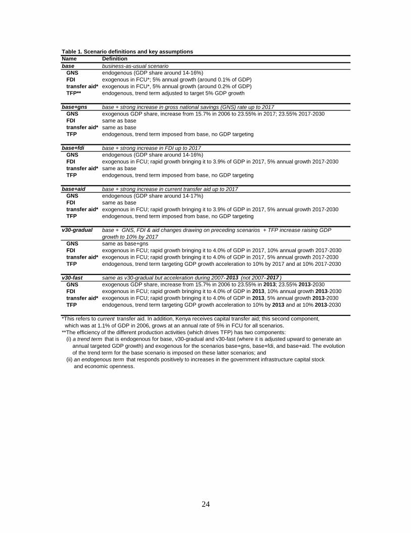
scenarios are defined in summary form in Table 1. The base scenario provides a

benchmark for comparison. The other simulations explore macro aspects of the growth

objectives of Vision 2030.

Turning to Table 1, the first three non-base simulations (BASE+GNS, BASE+FDI, and

BASE+ AID) analyze the impact of gradual but substantial increases in savings, FDI, and

aid, respectively. The objective is to understand the ceteris paribus impact of each of

these sources of growth on macro variables of interest. Directly or indirectly, changes in

each of these areas have a positive impact on growth and welfare. The increases are

strongest during the period 2007-2017, after which they follow the pace of economic

growth. The scenario V30-GRADUAL combines the preceding changes with a path of

TFP growth that permits GDP growth to increase gradually to 10% per year by 2017 and

stay at this rate up to 2030. V30-FAST imposes the same increases as for V30-

GRADUAL but during a more compressed time span, 2007-2013, after which growth is

maintained at 10%.

BASE

This scenario provides a benchmark to which other simulations are compared. It is

designed to maintain the current policy position and relative roles of private and

11

government sectors. Extrapolating on the relatively positive performance of Kenya’s

economy during the last few years, this scenario imposes an annual GDP growth rate of

5% during the period 2007-2030. Agricultural land under cultivation is assumed to grow

at a rate of 1% per year. The trend term for TFP growth is fine-tuned to generate the GDP

growth that is imposed, considering the impact of other growth determinants.11

For the government, service production, and capital stocks grow at the same rates.

Government consumption is the main source of demand for these services, complemented

by private sector demand. Outside of infrastructure, the observed 2006 GDP shares for

consumption in each subsector are maintained throughout the simulation period.

Government investment is driven by the need for government capital, given the simulated

evolution of government production in these sectors. For government infrastructure

investment spending (the major part) increases as a share of GDP from 0.5% in 2006 to

2.7% in 2030 while consumption spending (representing operation and maintenance)

grows in proportion to growth in the infrastructure capital stock.

Among government receipts, net transfers from domestic households are a fixed share of

GDP, using 2006 shares. Current and capital transfers from the rest of the world are fixed

in foreign currency, growing at an annual rate of 5%. The government also receives some

minor capital incomes. Domestic and foreign government borrowing are fixed at levels

such that, in the absence of exchange rate changes, growth in the related debt stocks

would coincide with the rate of GDP growth, i.e., the debt-GDP ratios would not change

over time. As we will see, given that exchange rate changes are minor, simulated

outcomes are very close to maintaining these ratios unchanged. Real domestic and

foreign interest rates are set at 2.5% and 2.6%, respectively, drawing on data on interest

payments, debt stocks and inflation. Among taxes, the rates of import tariffs are fixed

over time (at 2006 rates); as a result, the share of import tariff revenues in GDP will

depend on how rapidly import values (in domestic currency) grow relative to the overall

economy. As already noted, the overall government budget is balanced via scaling of

11 Drawing on Kenyan and international data, throughout the simulations, the different activities are ranked as follows in terms of productivity growth: agriculture, industry, private services, and government services. See Martin and Mitra (2001, p. 412), Hertel and Martin (1999, p. 7) and Kets and Lejour (2003, p. 9).

12

domestic tax rates (both direct and indirect). This mechanism assures that government

outlays and receipts are equal in value.

Apart from government-related items (referred to above), the balance of payments

includes private transfers and FDI. In 2006, transfers from the rest of the world to

households (including worker remittances) were estimated at 7.1% of GDP whereas FDI,

at 0.1% of GDP, was negligible.12 Over time, both inflows are assumed to grow at rates

that keep their GDP shares roughly unchanged. As explained above, the balance of

payments is cleared via adjustments in the real exchange rate whereas the model assures

that the remaining macro constraint, the savings-investment balance, is satisfied via

adjustments in private investment: its value is determined by available funding, defined

as the difference between private savings and government borrowing, supplemented by

FDI inflows.

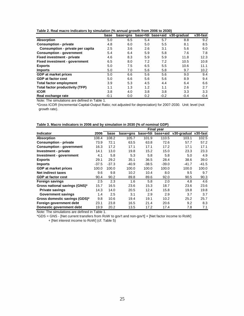
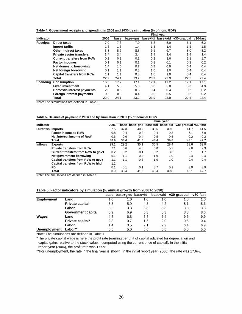
The results for the BASE scenario are found in Tables 2-6 (along with the results of the

other scenarios in the first set). All in all, driven by the assumed, relatively rapid 5% rate

of annual GDP growth, these results represent a significant improvement relative to

recent long-run trends for Kenya’s economy. Annual growth in most other macro

aggregates is also close to 5% (Table 2). The only exception is government investment,

for which annual growth is around 6.5%, reflecting increased spending on infrastructure.

Annual real GDP growth may be decomposed into 3.9% of growth on total factor

employment and 1.1% of TFP growth. The (gross) ICOR for the full period is 3.8.

Expressed as shares of GDP (Table 3), the changes for the different macro aggregates are

quite minor, an outcome that reflects a combination of similar real growth rates and

moderate relative price changes. Among other things, the trade deficit remains at around

8-9% of GDP whereas total investment stays in the range of 18-19%, without any

significant changes in foreign or national savings. Final demand (both consumption and

investment) shifts slightly from the government to the private sector (echoing the

observed difference between the two in terms of real growth, seen in Table 2). Domestic

12 The figure for FDI is based on data for 2005.

13

and foreign government debts change by very little relative to GDP (among other things a

reflection of the fact that the changes in the exchange rate were small).

Taking a more detailed look at the government accounts, also expressed as GDP shares

(Table 4), the changes by the end of the simulation period (2030) relative to 2006 are also

quite minor. The main differences are that, on the spending side, domestic interest

payments are lower whereas, on the revenue side, foreign borrowing (exogenous) is

higher than in 2006.13 Reflecting the combined impact of these and other, smaller

changes, the two balancing domestic tax items are both slightly higher than in 2006. In

the balance of payments (Table 5), most items have already been discussed. The new

items do not show any major changes from the situation in 2006.14 Among the different

factors, growth (in employment) is most rapid for government capital, followed by labor

and private capital (Table 6). Wages (or rents) grow most rapidly for land with more

moderate growth for labor. The unemployment rate declines from 17.6% in 2006 to

6.4%, i.e. close to the minimum unemployment rate of 5% (Table 6).

BASE+GNS

The content of this scenario is summarized in Table 1. Its assumptions are the same as the

base with two exceptions. First, during the period 2007-2017, the share of GNS in GDP is

gradually raised by 50%, from 15.7% in 2006 to 23.6% in 2017, a share that is

maintained without change up to 2030. (Under the BASE scenario, the GNS rate

remained at 14-16% throughout the simulation period.) This increased is brought about

via an increased private savings rates. Secondly, GDP growth is endogenous, i.e., no

GDP target is imposed.

13 For foreign borrowing, the difference is due to that 2006 GDP share was not compatible with a long-run, stable, foreign-debt to GDP ratio. For domestic interest rates, the change reflects a methodological issue: the model is a real model without inflation whereas these interest payments in 2006 were made in a setting with substantial inflation. Given this, interest rates were adjusted downwards to what were deemed appropriate real rates starting from 2007. 14 There is one exception, the item labeled as “capital grants” from rest of world to household. This is a residual item in the preliminary 2006 database that was difficult to classify – in all simulations, it was reduced gradually to zero by 2017 a level at which it stayed during the rest of the simulation period.

14

The rationale for this simulation is that rates of national savings, investment, and growth

are highly correlated and that, for high-investment economies, it is rare that foreign

savings finance more than 20% of investment (Schmidt-Hebbel and Servén, 1997, pp. 9-

13; Rodrik 2000, p. 481). Given this, it is hard to imagine a rapid growth scenario without

high national savings rates. However, higher savings rates are not likely to instigate more

rapid growth but are rather prerequisites for the sustainability of a growth acceleration

that is under way, reducing reliance on more uncertain foreign private and public capital

flows (Rodrik 2000, p. 505; Loayza et al. 2000, p. 394). International evidence also

indicates that private savings rates show inertia and that they are likely to rise in response

to higher per-capita incomes, rapid growth, and a lowering of the dependency ratio

(Loayza et al. 2000, pp. 399-402; Elbadawi and Mwega, 2000, p. 438). In Kenya, the

financial sector is relatively highly developed. The GNS rate peaked in 1993 at 20.5%

and ranged between 12% and 16% during the period 2002-2005 (World Bank 2007).

After this decline, Kenya is now classified as having a low savings rate relative to other

African countries (Ben Hammouda and Osakwe, 2006, p. 7).15

This change in the GNS rate translates into a substantial increase in the private sector

savings rate (out of post-tax incomes), from 16% to 25%. The economywide

repercussions are strong. Private investment growth expands by an additional 3.7

percentage points per year compared to BASE, raising growth in private capital stocks by

2.6 percentage points and total factor employment by 1.5 percentage points. Growth in

real GDP and other macro aggregates accelerate by 1.6 and 0.9-2.5 percentages points,

respectively, with the most rapid growth for exports. TFP growth increases moderately,

reflecting increased growth in infrastructure capital and a more open economy. On the

other hand, the ICOR increases to 4.0, a reflection of that the disproportionate increase in

private capital stock growth drives down the marginal productivity of private capital.

Expansion in imports is slightly more rapid than GDP growth, requiring a stronger export

expansion (in terms of percentage points) given Kenya’s trade deficit and the absence of

additional changes in the non-trade items in the balance of payments. Growth in real

household consumption per capita increases by 1.2 percentage points, to 3.6% per year.

15 In 2003, among 134 countries with data on GNS relative to GDP, Kenya ranked 85.

15

However, as will be discussed below, during the first few years of the simulation period,

household consumption suffers as a result of the increase in household savings. Given

that domestic and foreign borrowing (the latter in FCU) throughout the simulations are

kept at base levels, the GDP shares for the related debt stocks decline in proportion to the

extent of the acceleration in GDP growth. Factor wage growth increases for labor and

land whereas profit rate growth for private capital declines considerably, a reflection of

more rapid growth in the private capital stock. Government investment and capital also

expand more rapidly, driven by more rapid growth in GDP and government consumption

(Table 6). The unemployment rate falls to its minimum.

BASE+FDI

This scenario explores the impact of increases in FDI, a source of investment financing

that is more volatile but that, given this, also may increase more rapidly. The

distinguishing assumptions of this scenario are stated in Table 1. Apart from relaxing the

investment financing constraint, FDI may be more productive than domestic investment

and bring technological progress. The fact that Asian investments in SSA are growing

rapidly is a reason for being optimistic about future FDI growth. However, so far FDI in

SSA has been concentrated in terms of countries (primarily South Africa, Nigeria and the

Sudan) and sectors (mostly oil and gas) (Ben Hammouda and Osakwe, 2006, p. 13). FDI

in manufacturing could generate more significant employment growth. The factors that

could attract more FDI in manufacturing and other sectors, both in Kenya and in SSA in

general, include improvements in infrastructure, human capital, and governance, as well

as a more diversified production structure (Ndulu, 2007, p. 132; Dupasquier and Osakwe,

2005, pp. 17-19; Ben Hammouda and Osakwe, 2006, p. 13; EIU, 2006, pp. 38-39).

This simulation addresses the role of FDI as a source of investment financing; it does not

consider potential productivity gains from FDI. We incorporate such gains (without

explicitly ascribing them to FDI or any other specific source) in the scenarios that

combine an increase in FDI and other changes with a TFP increase). An increase in FDI

differs from an investment increase financed from domestic resources in two respects. On

16

one side, it does not require any immediate sacrifice of consumption for future benefit.

On the other side, the resulting increase in the private capital stock will be owned by

foreigners (not by domestic households), leading to higher profit remittances to the rest of

the world in future years.

Under the BASE scenario, the share of FDI in GDP at market prices was about 0.1%

throughout the period 2006-2030, corresponding to an annual growth rate of 5% in

foreign currency. Under BASE+FDI, growth is accelerated considerably, gradually

bringing FDI up to close to 4% of GDP during the period 2007-2017, after which it

continues to grow at an annual rate of 5%, maintaining a GDP share that remains close to

4%. This target level (around 4% of GDP) seems feasible given that many developing

countries, including some in sub-Saharan Africa, currently are at or above this share

(World Bank 2007). At the same time, it represents a drastic increase relative to the status

quo. In terms of 2003 US$, this corresponds to an increase from 16 million in 2006 to 1.1

billion in 2017.

The impact of this change is smaller in magnitude than for BASE+GNS but qualitatively

similar in several respects: real GDP growth increases substantially (by 0.6 percentage

points; Table 2). Among the national account aggregates, real growth acceleration is

relatively fast for private investment (which includes FDI) and relatively slow for private

consumption. Compared to BASE+GNS, the exchange rate depreciates slightly,

reflecting the fact that profit remittances, starting from 2015, exceed FDI, bringing about

a larger gap between the growth rates for exports and imports. Given this, growth in

absorption (total domestic final demand) accelerates less strongly than GDP. In terms of

GDP shares (Table 3), exports and private investment increase between 2006 and 2030

while the decreases are sharp for private consumption and more moderate for imports.

Given more rapid GDP growth and unchanged borrowing, the GDP shares for foreign

and domestic government debt decline. (The declines in the GDP shares for imports and

the foreign debt are mitigated by exchange rate depreciation.)

17

The changes in the GDP shares of the different items in the government budget are

relatively minor (Table 4). In the balance of payments (Table 5), profit remittances

(factor incomes sent to the rest of the world) increase from less than 1% of GDP in 2006

to more than 9% in 2030, a share that exceeds that of FDI, which in 2030 is at 3.7% of

GDP. The fact that profit remittances exceed FDI inflows puts the balance of payments

deficit. In the absence of any changes in non-trade flows relative to the base scenario, this

requires a decline in the trade deficit, from some 8% in 2006 to 2% in 2030, reducing the

gains in domestic absorption and welfare. Private consumption growth is only slightly

more rapid under this scenario than for the BASE. Compared to BASE+GNS, slower

private investment growth reduces private capital accumulation and raises profit rates.

Land and labor wage growth are slower given slower GDP growth whereas the

unemployment rate ends up slightly above the 5% minimum (Table 6). All in all, this

scenario suggests that the welfare gains from FDI maybe negligible unless FDI

contributes to more rapid TFP growth, a consideration that is incorporated in the

simulations V30-GRADUAL and V30-FAST.

BASE+AID

As noted above, additional aid (in grant form) relaxes the budget constraint of the

government, permitting expansion of government spending or a reduction in government

intake from other sources (taxes or borrowing). The second alternative permits more

rapid growth in private consumption, savings, and investment, adding to household well-

being and GDP. Whether it is preferable to expand spending or reduce other receipts

depends on the development objectives of the government and the relative efficiency of

resource use in the private and government sectors. In the scenario BASE+AID, we use

the aid to reduce taxes.16

Under this scenario, the component of aid that is raised is represented by current transfers

to the government (“official transfers” in the balance of payments), in 2006

16 Scenarios addressing the impact of alternative scenarios for aid-financed government expansion will be addressed in a separate paper.

18

corresponding to 0.2% of GDP (or approximately US$1 per capita). Under the BASE

scenario, official transfers grow at an annual rate of 5%, leaving its small share in GDP

roughly unchanged. As stated in Table 1, under BASE+AID, growth is accelerated

considerably, gradually bringing official grants up to close to 4% of GDP during the

period 2007-2017, after which it continues to grow at an annual rate of 5%, maintaining a

GDP share that remains close to 4%. This is the same target level (in FCU) that was

imposed for FDI in the preceding simulations – it also seems appropriate for similar

reasons: it is feasible (similar or higher shares are obtained by many countries in sub-

Saharan Africa; World Bank 2007) but perhaps biased on the optimistic side (considering

the current GDP share). Expressed in terms of 2003 US$, this corresponds to an increase

from 23 million in 2006 to more than 1.2 billion in 2017 (almost US$25 per capita), at

which point these transfers continue growing at 5% per year. The government is assumed

to use these additional aid receipts to finance a uniform scaling down of direct and

indirect tax rates. The households are assumed to allocate the gains from the direct tax cut

to savings – in effect, the foreign aid increase permits the government to continue doing

what it did before (in terms of GDP shares) while simultaneously cutting direct taxes.

As shown in Table 2, this aid increase has a positive effect on annual GDP growth, which

accelerates by 0.6 percentage points. Among the macro aggregates, private investment

growth expands most strongly, by 1.3 percentage points, whereas the other items register

increases of 0.5-0.8 percentage points, i.e., the government is increasing its consumption

and investment in response to the increase in GDP growth. As a result of the aid increase,

the trade deficit expands, permitting absorption to grow slightly more rapidly than GDP.

In terms of macro-level GDP shares (Table 3), the main effect of this aid increase

(comparing to the situation in 2030 for BASE) are increases in private investment and

imports, and a decrease in exports. This outcome reflects the fact that the aid (a) is used

to cut direct taxes and raise private savings; and (b) relaxes the foreign exchange

constraint, permitting a larger trade deficit. More rapid growth, unchanged borrowing,

and exchange rate appreciation together reduce the GDP shares for the government’s

foreign and domestic debt stocks. These changes are also reflected in the government

19

budget (Table 4), where the aid transfers become more important while the significance

of taxes diminish. In the balance of payments, also compared to the BASE, the aid

increase makes it possible for Kenya to import more and export less without facing the

burden of increased profit remittances out of the country (as in BASE+FDI) (Table 5).

The effects on factor employment and unemployment, wages, and the profit rate are very

similar to BASE+FDI (Table 6).

The three scenarios BASE+GNS, BASE+FDI, and BASE+AID all bring about increased

private investment. Relative to BASE, BASE+AID avoids the slow-down in private

consumption growth that characterizes BASE+GNS (until 2015) and the burden of future

repayments that was associated with BASE+FDI, as higher foreign investments lead to

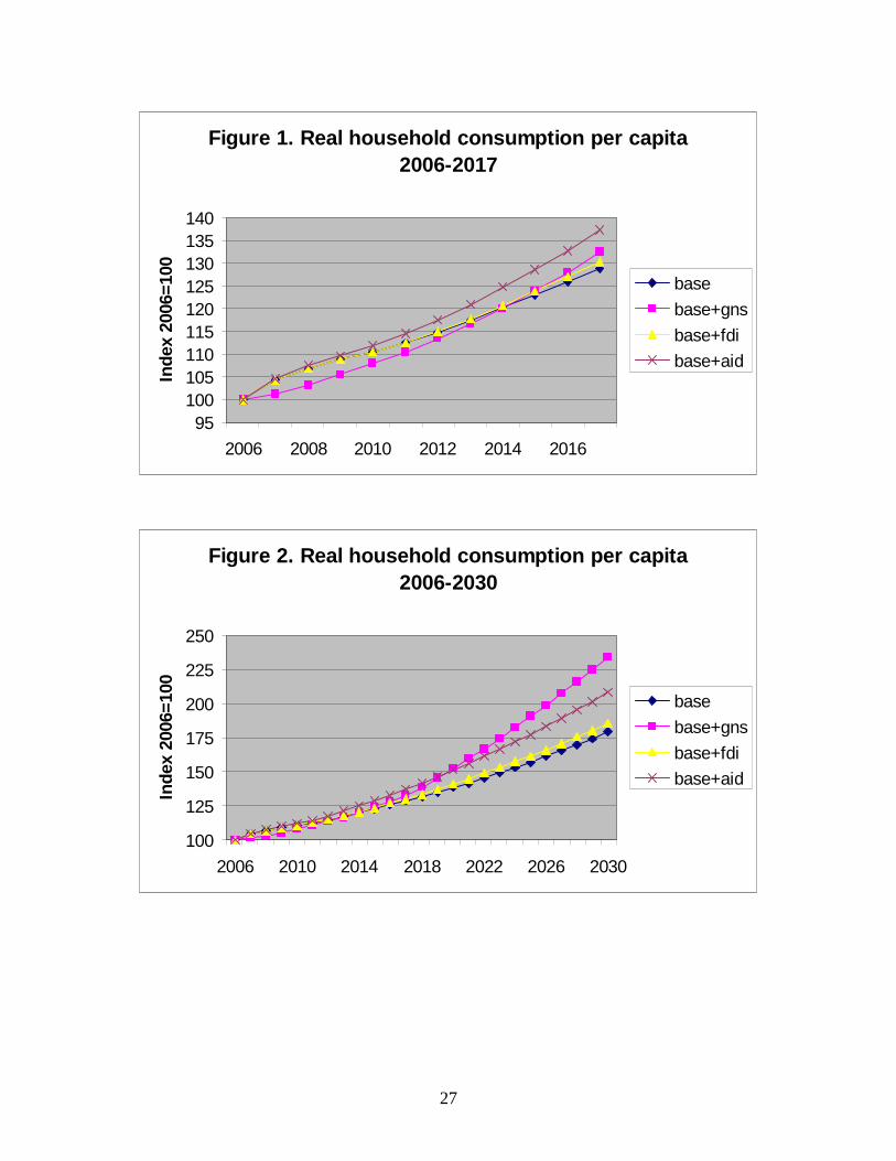
foreign ownership of the domestic capital stock. Figures 1 and 2 compares the evolution

or real household consumption per capita for BASE and these three scenarios during the

subperiod 2006-2017 and for the full simulation period, 2006-2030. As shown in Figure

1, BASE+AID generates higher household consumption than the other scenarios up to

2020. Up to 2015, BASE+GNS has the lowest level of household consumption (as

households sacrifice consumption for higher savings). However, starting from 2020, the

cumulative growth payoffs from higher savings permit BASE+GNS to dominate the

other three scenarios.

V30-GRADUAL

The individual changes simulated so far have all had a positive but still quite moderate

impact, unable to raise GDP growth up to the targeted 10% rate. They have primarily

influenced growth by raising private capital accumulation; their impact on TFP growth

has been minor. In this scenario, V30-GRADUAL, we bring together the three preceding

changes (increases in aid, private savings, and FDI) and combine these with an

acceleration in TFP growth that is sufficient to gradually raise annual GDP growth to

10% during the period 2007-2017, after which it stays at this elevated rate. The details

are stated in Table 1. It is reasonable to raise TFP growth in conjunction with these other

20

changes given that more rapid growth in savings, investment, FDI, and TFP are likely to

come hand in hand. We do not ascribe the TFP increase to any specific source.

Accelerating TFP growth may require some combination of reductions in transactions

costs, support for innovations, and improvements in skills and institutions. For Kenya,

indirect costs (i.e., costs of security, transactions, and other items unrelated to the core

production process in the factory), impose a particularly heavy burden, reducing Kenya’s

competitiveness relative to other countries (Ndulu 2007, p. 64).

By construction, the new scenario generates the targeted rates of GDP growth. For the

period 2007-2030 as a whole, this translates into an annual growth rate of 8.9%. TFP

grows at 2.6% per year, an increase of 1.5 percentage points compared to the BASE;

factor employment growth also accelerates. Other macro aggregates grow at annual rates

of 7-12% with the highest rate for private investment, which is driven by the increases in

GNS and FDI. In response to the increases in aid and FDI, the real exchange rate

appreciates at a rate of 0.4% per year. At the macro level, the GDP share of private

investment increases at the expense of private consumption, a change that follows from

the increase in private (and total national) savings (Table 3). Relative to GDP, domestic

and foreign government debts decline more strongly than for the preceding scenarios.

In the government budget, also measured relative to GDP (Table 4), the changes

compared to BASE are moderate. On the revenue side, they reflect the effects of

increased aid (reducing the need for taxes) and more rapid growth (reducing the GDP

shares for foreign and domestic borrowing, which were fixed in foreign and domestic

currency, respectively). In addition to what already has been noted, the balance of

payments (Table 5) shows that, in the final year, the FDI inflow falls short of profit

remittances (labeled “factor income to RoW”). Private transfers from the rest of the

world, which grow at an annual rate of 2% per capita, also decline in importance given

very rapid GDP growth and the fact that exchange rate appreciation reduces their value in

domestic currency. As far as factors are concerned, still compared to BASE, the

combined scenario generates a stronger expansion in private capital accumulation and

21

slower growth in profit rates. Wages grow more rapidly for labor and land while the

unemployment rate declines to its minimum (Table 6). More rapid GDP growth leads to

more rapid growth in government investment and capital stocks.

Figures 3 and 4 shows the evolution of the GDP shares for investment (divided into

private and government) and savings (divided into [gross] national and foreign) for the

simulations BASE and V30-GRADUAL, respectively.17 The main difference between the

two scenarios is that, under V30-GRADUAL, the GDP shares for national savings and

private investment increase gradually between 2006 and 2017, after which they stabilize

at these higher levels. In parallel, there is a corresponding decrease in the GDP share of

private consumption. In real terms, the four items in the graph and private consumption

all grow more rapidly under V30-gradual but, as indicated by the two Figures, the relative

growth accelerations are larger for private investment and national savings.

V30-FAST

This scenario is similar to V30-GRADUAL except for the fact that the acceleration is

more rapid, taking place during the period 2007-2013 instead of 2007-2017 (cf. Table 1).

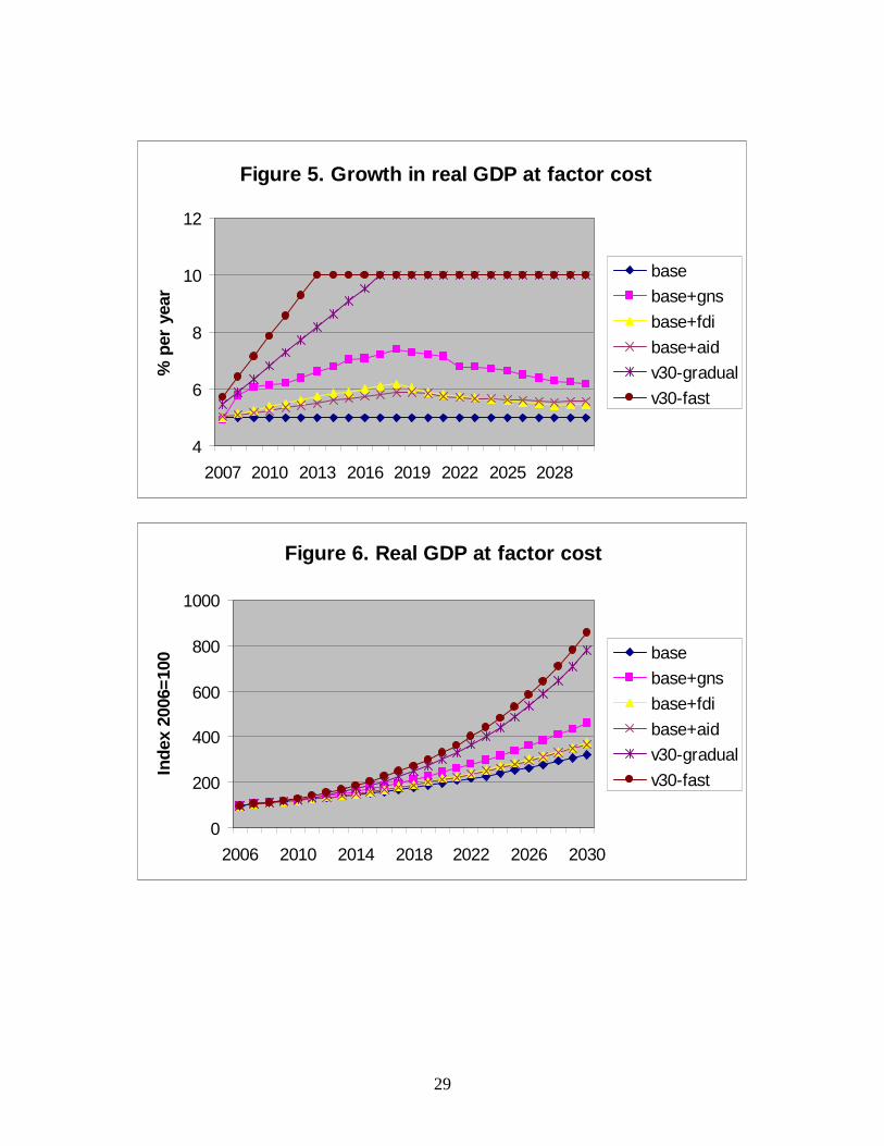
This growth target is clearly extremely ambitious. Figure 5 compares the path of annual

growth in real GDP at factor cost across the different simulations. For this simulation, it

is assumed that, after 2013, FDI and current aid transfers continue to grow at rates of

10% and 5%, respectively while GNS stays at 23.5% of GDP.

As shown in Table 2, compared to V30-GRADUAL, the acceleration in GDP growth

may be attributed to a combination of increased TFP growth (by 0.1 percentage points)

and factor employment (by 0.2 percentage points). Real growth for the other macro

aggregates increases by 0.2-0.5 percentage points. In terms of GDP shares, the changes

compared to V30-GRADUAL are relatively minor for the different items in the macro

accounts, the government budget and the balance of payments (Tables 3-5).

17 Note that the sum of the two investment shares equals the sum of the two savings shares.

22

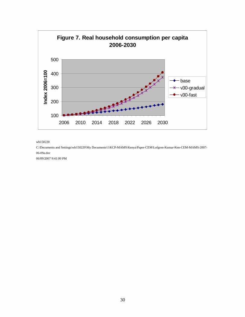
Figures 6-7 provides an over-all perspective of the ambitious nature of Vision 2030 by

showing total real GDP (at factor cost) and household consumption per capita for

selected simulations. Compared to the BASE simulation, Vision 2030 strives for a

revolution in economic performance. As shown in Figure 6, the size of the economy

(measured by total real GDP) in 2030 relative to 2006 increases by 680% for the scenario

V30-GRADUAL and 760% for the scenario V30-FAST, as opposed to a 220% increase

for the BASE scenario, which remains optimistic relative to Kenya’s long-run record) –

during the most recent 24-year period, 1981-2005, the size of the economy only increased

by 106% (World Bank 2007).

Similarly, according to Figure 7, real household consumption per capita increases by

around 275% for V30-GRADUAL and 310% for V30-FAST, as opposed to 80% for the

BASE scenario. During the period 1981-2005, the same indicator grew by a mere 16%

(World Bank 2007)

REFERENCES

Ben Hammouda, Hakim, and Patrick N. Osakwe (2006). “Financing Development in Africa: Trends, Issues and Challenges.” ATPC Work in Progress No. 48, Economic Commission for Africa, Addis Ababa. Dessus, Sébastien and Rémy Herrera (1996). “Le Rôle du Capital Public dans la Croissance des Pays en Développement au Cours des Années 80.” Working Paper 115. OECD Development Centre. Dupasquier, Chantal, and Patrick N. Osakwe (2005). “Foreign Direct Investment in Africa: Performance, Challenges and Responsibilities.” ATPC Work in Progress No. 21, Economic Commission for Africa, Addis Ababa. EIU (Economist Intelligence Unit) (2006). Kenya: Country Profile 2006. Elbadawi, Abraham A., and Francis M. Mwega (2000). “Can Africa's Saving Collapse Be Reversed?” World Bank Economic Review, Vol. 14, No. 3, pp. 415-43. Hertel, Thomas W. and Will Martin (1999) “Would Developing Countries Gain from

23

Inclusion of Manufactures in the WTO Negotiations?” Paper to be presented at the Conference on WTO and The Millennium Round, Geneva, September 20-21. Kets, Willemien, and Arjan Lejour (2003). Sectoral TFP Developments in the OECD. CPB Netherlands Bureau for Economic Policy Analysis. Memorandum 58. Loayza, Norman, Klaus Schmidt-Hebbel, and Luis Servén (2000). “Saving in Developing Countries: An Overview.” World Bank Economic Review. Vol. 14, No. 3: 393-414 Martin, Will, and Devashish Mitra (2001). “Productivity Growth and Convergence in Agriculture” Economic Development and Cultural Change, Vol. 49, No. 2, pp. 403-422 Ndulu, Benno, with Lopamudra Chakraborti, Lebohang Lijane, Vijaya Ramachandran, and Jerome Wolgin (2007). Challenges of African Growth: Opportunities, Constraints, and Strategic Directions. Washington, D.C.: World Bank Rodrik, Dani (2000). “Saving Transitions.” World Bank Economic Review, Vol. 14, No. 3: 481-517 Schmidt-Hebbel, Klaus, and Luis Servén (1997). “Saving across the World Puzzles and Policies.” World Bank Discussion Paper No. 354. The World Bank, Washington, D.C. Tahari, Amor, Dhaneshwar Ghura, Bernardin Akitoby, and Emmanuel Brou Aka (2004) “Sources of Growth in Sub-Saharan Africa”. IMF Working Paper 176. World Bank (2007). World Development Indicators.

24

Table 1. Scenario definitions and key assumptionsName Definitionbase business-as-usual scenario

GNS endogenous (GDP share around 14-16%)FDI exogenous in FCU*; 5% annual growth (around 0.1% of GDP)transfer aid* exogenous in FCU*, 5% annual growth (around 0.2% of GDP)TFP** endogenous, trend term adjusted to target 5% GDP growth

base+gns base + strong increase in gross national savings (GNS) rate up to 2017GNS exogenous GDP share, increase from 15.7% in 2006 to 23.55% in 2017; 23.55% 2017-2030FDI same as basetransfer aid* same as baseTFP endogenous, trend term imposed from base, no GDP targeting

base+fdi base + strong increase in FDI up to 2017GNS endogenous (GDP share around 14-16%)FDI exogenous in FCU; rapid growth bringing it to 3.9% of GDP in 2017, 5% annual growth 2017-2030transfer aid* same as baseTFP endogenous, trend term imposed from base, no GDP targeting

base+aid base + strong increase in current transfer aid up to 2017GNS endogenous (GDP share around 14-17%)FDI same as basetransfer aid* exogenous in FCU; rapid growth bringing it to 3.9% of GDP in 2017, 5% annual growth 2017-2030TFP endogenous, trend term imposed from base, no GDP targeting

v30-gradual base + GNS, FDI & aid changes drawing on preceding scenarios + TFP increase raising GDP growth to 10% by 2017

GNS same as base+gnsFDI exogenous in FCU; rapid growth bringing it to 4.0% of GDP in 2017, 10% annual growth 2017-2030transfer aid* exogenous in FCU; rapid growth bringing it to 4.0% of GDP in 2017, 5% annual growth 2017-2030TFP endogenous, trend term targeting GDP growth acceleration to 10% by 2017 and at 10% 2017-2030

v30-fast same as v30-gradual but acceleration during 2007- 2013 (not 2007- 2017 )GNS exogenous GDP share, increase from 15.7% in 2006 to 23.55% in 2013; 23.55% 2013-2030FDI exogenous in FCU; rapid growth bringing it to 4.0% of GDP in 2013, 10% annual growth 2013-2030transfer aid* exogenous in FCU; rapid growth bringing it to 4.0% of GDP in 2013, 5% annual growth 2013-2030TFP endogenous, trend term targeting GDP growth acceleration to 10% by 2013 and at 10% 2013-2030

*This refers to current transfer aid. In addition, Kenya receives capital transfer aid; this second component, which was at 1.1% of GDP in 2006, grows at an annual rate of 5% in FCU for all scenarios.**The efficiency of the different production activities (which drives TFP) has two components: (i) a trend term that is endogenous for base, v30-gradual and v30-fast (where it is adjusted upward to generate an annual targeted GDP growth) and exogenous for the scenarios base+gns, base+fdi, and base+aid. The evolution of the trend term for the base scenario is imposed on these latter scenarios; and (ii) an endogenous term that responds positively to increases in the government infrastructure capital stock and economic openness.

25

Table 2. Real macro indicators by simulation (% annual growth from 2006 to 2030)base base+gns base+fdi base+aid v30-gradual v30-fast

Absorption 5.0 6.5 5.4 5.7 8.8 9.2Consumption - private 4.8 6.0 5.0 5.5 8.1 8.5

Consumption - private per capita 2.5 3.6 2.6 3.1 5.6 6.0Consumption - government 5.4 6.4 5.9 5.8 7.6 7.8Fixed investment - private 4.6 8.3 5.9 5.9 11.8 12.3Fixed investment - government 6.5 8.0 7.2 7.2 10.5 10.8Exports 5.0 7.5 6.5 5.5 10.6 11.1Imports 5.0 7.0 5.6 5.8 9.7 10.2GDP at market prices 5.0 6.6 5.6 5.6 9.0 9.4GDP at factor cost 5.0 6.6 5.6 5.6 8.9 9.4Total factor employment 3.9 5.3 4.5 4.4 6.4 6.6Total factor productivity (TFP) 1.1 1.3 1.2 1.1 2.6 2.7ICOR 3.8 4.0 3.8 3.8 3.3 3.3Real exchange rate -0.1 0.0 0.2 -0.2 -0.4 -0.4Note: The simulations are defined in Table 1.*Gross ICOR (Incremental Capital-Output Ratio; not adjusted for depreciation) for 2007-2030. Unit: level (not growth rate).

Table 3. Macro indicators in 2006 and by simulation in 2030 (% of nominal GDP)

Indicator 2006 base base+gns base+fdi base+aid v30-gradual v30-fastAbsorption 108.4 108.2 105.7 101.9 110.5 103.1 102.5Consumption - private 73.9 72.1 63.5 63.8 72.6 57.7 57.2Consumption - government 16.3 17.2 17.1 17.1 17.2 17.1 17.1Investment - private 14.1 13.0 19.8 15.2 15.0 23.3 23.3Investment - government 4.1 5.8 5.3 5.8 5.8 5.0 4.9Exports 29.1 29.2 35.1 36.5 28.4 38.6 39.0Imports -37.5 -37.3 -40.9 -38.5 -39.0 -41.7 -41.5GDP at market prices 100.0 100.0 100.0 100.0 100.0 100.0 100.0Net indirect taxes 9.6 9.8 10.2 10.4 8.0 9.5 9.7GDP at factor cost 90.4 90.2 89.8 89.6 92.0 90.5 90.3Foreign savings 2.5 2.3 1.6 5.8 2.0 4.8 4.6Gross national savings (GNS)* 15.7 16.5 23.6 15.3 18.7 23.6 23.6

Private savings 14.3 14.0 20.5 12.4 15.8 19.8 19.8Government savings 1.4 2.5 3.1 2.9 2.9 3.7 3.7

Gross domestic savings (GDS)* 9.8 10.6 19.4 19.1 10.2 25.2 25.7Foreign government debt 23.1 23.8 16.5 21.4 20.6 9.2 8.3Domestic government debt 19.9 20.2 13.5 17.2 17.4 7.8 7.1Note: The simulations are defined in Table 1.*GDS = GNS - [Net current transfers from RoW to gov't and non-gov't] + [Net factor income to RoW] + [Net interest income to RoW] (cf. Table 5)

Final year

26

Table 4. Government receipts and spending in 2006 and 2030 by simulation (% of nom. GDP)

Indicator 2006 base base+gns base+fdi base+aid v30-gradual v30-fastReceipts Direct taxes 7.0 7.3 7.0 6.8 5.9 6.1 6.2

Import tariffs 1.3 1.3 1.4 1.3 1.4 1.5 1.5Other indirect taxes 8.3 8.5 8.8 9.1 6.7 8.0 8.2Private sector transfers 3.4 3.4 3.4 3.4 3.4 3.4 3.4Current transfers from RoW 0.2 0.2 0.1 0.2 3.6 2.1 1.7Factor incomes 0.1 0.1 0.1 0.1 0.1 0.2 0.2Net domestic borrowing 1.4 1.0 0.7 0.9 0.9 0.4 0.4Net foreign borrowing 0.1 1.1 0.8 1.0 1.0 0.4 0.4Capital transfers from RoW 1.1 1.1 0.8 1.0 1.0 0.4 0.4Total 22.9 24.1 23.2 23.9 23.9 22.5 22.4

Spending Consumption 16.3 17.2 17.1 17.1 17.2 17.1 17.1Fixed investment 4.1 5.8 5.3 5.8 5.8 5.0 4.9Domestic interest payments 2.0 0.5 0.3 0.4 0.4 0.2 0.2Foreign interest payments 0.6 0.6 0.4 0.5 0.5 0.2 0.2Total 22.9 24.1 23.2 23.9 23.9 22.5 22.4

Note: The simulations are defined in Table 1.

Final year

Table 5. Balance of payment in 2006 and by simulation in 2030 (% of nominal GDP)

Indicator 2006 base base+gns base+fdi base+aid v30-gradual v30-fastOutflows Imports 37.5 37.3 40.9 38.5 39.0 41.7 41.5

Factor income to RoW 0.8 0.4 0.2 9.4 0.3 6.1 6.0Net interest income of RoW 0.6 0.6 0.4 0.5 0.5 0.2 0.2Total 38.9 38.4 41.5 48.4 39.8 48.1 47.7

Inflows Exports 29.1 29.2 35.1 36.5 28.4 38.6 39.0Private transfers from RoW 7.1 6.6 4.6 6.0 5.7 2.6 2.3Current transfers from RoW to gov't 0.2 0.2 0.1 0.2 3.6 2.1 1.7Net government borrowing 0.1 1.1 0.8 1.0 1.0 0.4 0.4Capital transfers from RoW to gov't 1.1 1.1 0.8 1.0 1.0 0.4 0.4Capital transfers from RoW to hhd 1.2FDI 0.1 0.1 0.1 3.7 0.1 3.9 3.9Total 38.9 38.4 41.5 48.4 39.8 48.1 47.7

Note: The simulations are defined in Table 1.

Final year

Table 6. Factor indicators by simulation (% annual growth from 2006 to 2030)base base+gns base+fdi base+aid v30-gradual v30-fast

Employment Land 1.0 1.0 1.0 1.0 1.0 1.0Private capital 3.3 5.9 4.3 4.2 8.1 8.6Labor 3.2 3.3 3.3 3.3 3.3 3.3Government capital 5.9 6.9 6.3 6.3 8.3 8.6

Wages Land 4.8 6.8 5.8 5.4 9.5 9.9Private capital* 2.3 0.7 1.6 2.0 0.6 0.4Labor 1.4 3.5 2.1 2.2 6.4 6.9

Unemployment Labor** 6.5 5.0 5.6 5.5 5.0 5.0Note: The simulations are defined in Table 1.*The private capital wage is here the profit rate (earning per unit of capital adjusted for depreciation and capital gains relative to the stock value, computed using the current price of capital). In the initial report year (2006), the profit rate was 17.9%.**For unemployment, the rate in the final year is shown. In the initial report year (2006), the rate was 17.6%.

27

Figure 1. Real household consumption per capita2006-2017

95100105110115120125130135140

2006 2008 2010 2012 2014 2016

Inde

x 20

06=1

00

base

base+gns

base+fdi

base+aid

Figure 2. Real household consumption per capita2006-2030

100

125

150

175

200

225

250

2006 2010 2014 2018 2022 2026 2030

Inde

x 20

06=1

00

base

base+gns

base+fdi

base+aid

28

Figure 3. BASE: Savings and investment

0

5

10

15

20

25

30

2006

2008

2010

2012

2014

2016

2018

2020

2022

2024

2026

2028

2030

% o

f G

DP Priv Inv

Gov Inv

For Sav

Nat Sav

Figure 4. V30-GRADUAL: Savings and Investment

0

5

10

15

20

25

30

2006

2008

2010

2012

2014

2016

2018

2020

2022

2024

2026

2028

2030

% o

f G

DP Priv Inv

Gov Inv

For Sav

Nat Sav

29

Figure 5. Growth in real GDP at factor cost

4

6

8

10

12

2007 2010 2013 2016 2019 2022 2025 2028

% p

er y

ear

base

base+gns

base+fdi

base+aid

v30-gradual

v30-fast

Figure 6. Real GDP at factor cost

0

200

400

600

800

1000

2006 2010 2014 2018 2022 2026 2030

Inde

x 20

06=1

00

base

base+gns

base+fdi

base+aid

v30-gradual

v30-fast

30

Figure 7. Real household consumption per capita2006-2030

100

200

300

400

500

2006 2010 2014 2018 2022 2026 2030

Inde

x 20

06=1

00

base

v30-gradual

v30-fast

wb150220

C:\Documents and Settings\wb150220\My Documents\1\KCP-MAMS\Kenya\Paper-CEM\Lofgren-Kumar-Ken-CEM-MAMS-2007-

06-09a.doc

06/09/2007 9:41:00 PM