Embed Size (px)
Citation preview
The Changing Relevance of Accounting Numbers to Debt Holders over Time
Dan Givoly
Pennsylvania State University
Carla Hayn University of California, Los Angeles
Sharon Katz Columbia University
June 2013
Abstract
We examine the change over time in the information content of accounting numbers from the perspective of bondholders and the causes for this change. Using proprietary longitudinal data, we find that, in contrast to the decline in the information content of accounting numbers to equity holders over time, the information content to bondholders has held steady or risen. The rise is attributable to economic factors such as an increase in risk and in the frequency of unfavorable news to which the valuation of debt is more sensitive than that of equity. There are indications, however, that reporting factors, specifically an increase in conservatism over the last four decades, is associated with this rise. The findings contribute to the scant literature on the use of financial information by bondholders and the extent to which financial reporting meets their unique information needs. Given debt holders prominence as users of financial statements, the findings have important implications for accounting standard setting.
____________________________
We appreciate the helpful comments of Dan Amiram, Fabrizio Ferri, Trevor Harris, Suresh Nallareddy, Doron Nissim, Gil Sadka and workshop participants at Columbia Business School and the 2013 EAA Annual Congress. We also gratefully acknowledge financial support provided by Columbia Business School and Harvard Business School. All errors are our own.
2
The Changing Relevance of Accounting Numbers to Debt Holders over Time
1. Introduction
With few exceptions, studies on the value relevance of earnings have been conducted from
the perspective of equity holders, using stock returns to gauge the value relevance or information
content of the reported numbers. This is also true for studies that have focused on the
information content of specific financial statement components such as revenues, cash flows,
accruals and earnings-related information such as earnings forecasts.
As an example of the focus on equity holders, the call for the capitalization of R&D and
various other intangibles often made in the recent debate about how best to account for
investments in intangibles generally takes the perspective of stockholders, noting that they view
such investments as assets (Lev and Sougiannis 1996; Aboody and Lev 1998). This perspective
fails to consider that the capitalization of intangibles, while enhancing the information content of
financial statements to equity holders, might diminish the information content for debt holders
(Shi 2003). Indeed, this “equity-perspective bias” permeates capital markets research designed to
assess the relative merits and capital market effects of alternative accounting principles.
Similarly, the research on the change over time in the information content of accounting
numbers has taken the perspective of equity holders by correlating these numbers with stock
prices or stock returns, ignoring the information content of these numbers to debt holders.
However, the research findings on how the value relevance of accounting numbers for equity
holders has changed over time does not necessarily extend to debt holders. Some of the most
important trends in financial reporting in recent decades, such as the shift to an asset-liability
focus (the so-called “balance sheet approach”) from a revenue-expense focus (the “income
statement” approach)and the move towards fair value accounting have different potential

3
implications for the usefulness and relevance of accounting numbers to equity holders and debt
holders.
The sensitivity of debt holders to accounting numbers is likely to differ from that of equity
holders. As often noted, equity holders of a public corporation can be viewed as holders of a put
option on the value of the firm. Accordingly, stock prices are expected to be less sensitive to
downward risk then to upward prospects. This expectation is consistent with the findings that
stock prices respond less to losses and earnings declines than they do to profits and earnings
increases.1 Debt holders, in contrast, can be viewed as having a call option on the firm’s assets.
Correspondingly, debt prices are expected to be less sensitive to upward prospects and more
affected by downside risk.
These different features of equity and debt securities suggest that debt holders would be
more concerned than equity holders with the ability of earnings and other accounting numbers to
adequately and promptly convey downside risks and unfavorable information. Therefore,
inferences regarding the informativeness of accounting numbers or the desirability of alternative
accounting principles may differ depending on whether the perspective adopted is that of equity
holders or debt holders.
The scarcity of research from the debt holders’ perspective cannot be explained by the
relatively low importance of debt in the capital markets since the aggregate debt and equity
investments are approximately equal in size. 2 ,3 Nor can the fact that research has focused
1 See Hayn (1995) and Burgstahler and Dichev (1997). 2 Among the few studies that adopt the debt holders’ perspective in evaluating the usefulness of accounting numbers are Ball et al. (2008), DeFond and Zhang (2009, 2011), Shi (2003), Easton et al. (2009), Elliott et al. (2010), Gkougkousi (2012), Khurana and Raman (2003), Plummer and Tse (1999), and Sridharan (2011). 3 The Securities Industry and Financial Markets Association reports that the market value of the U.S. corporate bond market was $7.9 trillion at the end of 2011 (see http://www.sifma.org/research/statistics.asp). Reliable information on the size of the private debt market is not available. However, it is estimated to be about $8.5 million in a steady state (assuming an average loan term of five years and an average annual aggregate loan amount of $1.7 trillion, the dollar value of private loans issued in the year ending June 15, 2012 (as reported by Thomson One). Combined, the
4
primarily on equity holders be explained by the underlying objectives of financial reporting as
stated by standard setters since they appear to give equal weight to creditors as users of financial
information for decision-making purposes.4
One explanation for the research focus on equity holders is the relative difficulty in
obtaining price and return data on debt as compared with equity issuances. Stock prices and
stock returns have been easily obtainable since the foundation of the Center for Research in
Security Prices (CRSP) in 1960. Currently, CRSP annual stock price data for companies traded
on the NYSE are available from December 1925 and daily data are provided beginning in July
1962. Return data for companies listed on AMEX and NASDAQ are available from,
respectively, 1962 and 1972. In contrast, bond data availability is more limited. The Mergent
Fixed Income Securities Database (FISD) contains bond exchange transactions beginning in
1994 but only for U.S. insurance companies. The Trade Reporting and Compliance Engine
(TRACE) Corporate Bond Database has bond prices beginning in 2002 with more
comprehensive data available only from 2005.
The objective of this study is to fill this gap in the research by examining the change over
time in the information content of accounting numbers to debt holders. Based on a sample of
more than 10,000 corporate bond issues extending over the 34-year period from 1975 to 2008,
this study demonstrates how the unique features of bonds affect the manner in which bond
total market value of public and private debt is thus approximately $16.4 trillion. This is slightly larger than the market value of equity which was estimated to be about $15.6 trillion at the end of 2011 (based on the World Federation of Exchanges report on the aggregate market value of shares traded on the NYSE, Euronext and NASDAQ OMX (see http://www.world-exchanges.org/statistics). 4 The FASB explicitly mentions debt holders noting that the objectives of financial statements are to provide useful information to “potential investors and creditors…in making rational investment, credit and similar decisions.” (See paragraphs 34-36, Statement of Concepts of Financial Statements No. 1, FASB 2008.) A similar objective is expressed in the conceptual framework of the IAS (1989) – The Conceptual Framework for Financial Reporting, which was subsequently adopted by the IASC in 2001, It states that among the primary users of financial reporting are “lenders and other creditors” who use that information to “make decisions about buying, selling or holding … debt instruments and providing or settling loans or other forms of credit” (see ibid OB2).

5
valuation and bond returns respond to accounting information. Using various measures, we find
that the information content of accounting numbers for bondholders has increased or stayed
steady over time while, consistent with previous studies, this content has generally decreased for
equity holders. Most of the increase is attributable to economic factors associated with an
increase in risk and with an increased frequency of unfavorable news to which the valuation of
debt is more sensitive than that of equity. However, we also find evidence consistent with the
notion that the increase in reporting conservatism over the last four decades, which likely reflects
changes in accounting standards and their implementation as well as changes in management
incentives, contributes to this trend.
The paper contributes to the literature in a number of ways. It is the first to estimate the
evolvement in the value-relevance of accounting numbers for debt holders and contrast it with
the change over time in the information content of these numbers for equity holders. The paper
also extends prior research that confirms empirically the theoretical predictions regarding the
differential response of the bond and stock markets to accounting information. Further, it shows
that increased reporting conservatism provides informational benefits to bondholders, a main
constituent of financial reporting. The findings have implications for accounting standard setters
and regulators in emphasizing the different implications of accounting standards for different
investor groups.
The paper proceeds as follows. In the next section, the difference in the valuation of
earnings numbers by equity and debt holders is discussed. Section 3 contains a review of the
literature on the accounting properties examined by this study. The methodology is presented in
Section 4, followed by a description of the data and sample in Section 5. The results are

6
presented and discussed in Section 6. The final section contains summary and concluding
remarks.
2. Valuation of Equity and Debt as a Function of Earnings
The discussion in this section assumes without loss of generality that expected earnings
correspond to expected cash flows. The relationship between reported earnings and equity
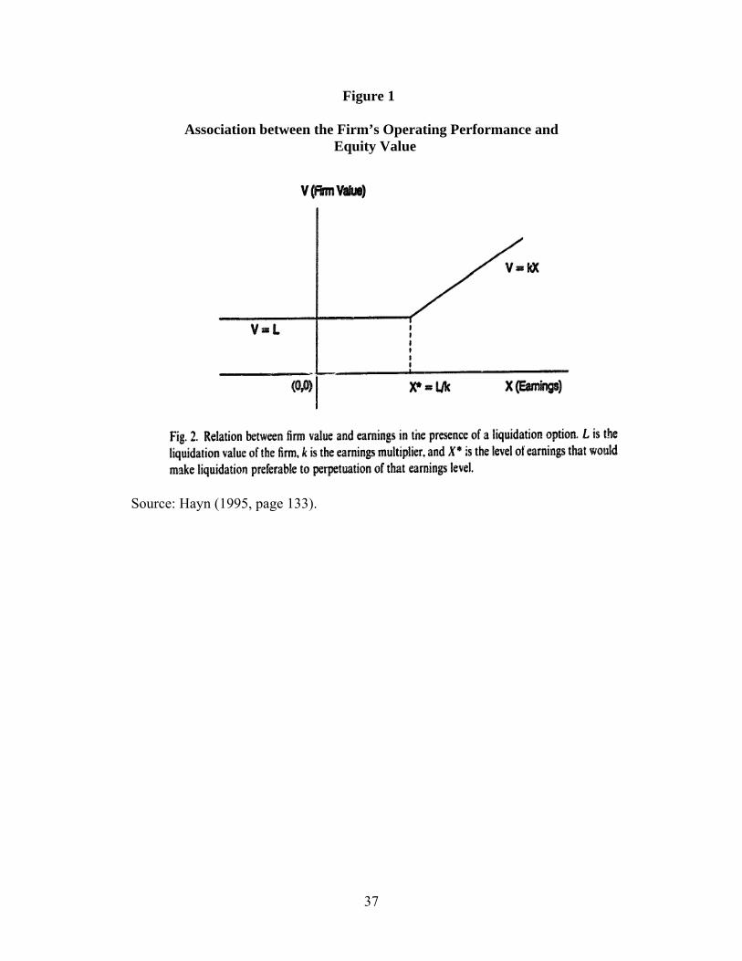
values is illustrated in figure 1 (from Hayn, 1995). As the figure indicates the value of equity
rises and falls with earnings. However, when earnings decline below a certain threshold that
represents the level of earnings that, when capitalized, equal the exit value of the firm’s equity,
their persistence is likely to trigger the liquidation (put) option by the equity holders. In other
words, earnings below this threshold level are not expected to perpetuate.
Figure 2 (from Fischer and Verrecchia, 2001) describes the association between reported
earnings and debt values. As the figure shows, debt values are positively related to earnings.
However, above a certain level of earnings, debt values become less sensitive to movements in
earnings. That is, the change in the value of debt is convex in earnings at low values of earnings
because debt holders, not equity holders, are the residual claimants. The value of debt is concave
at higher level of earnings because of the cap on the redemption value of the debt.
Given that the functional relation between earnings, book values and stock returns is differs
from that between earnings, book values and bond returns, the conclusions of studies on the
“information content of earnings” which rely on stock returns could well be different from those
using bond returns. Further, given that equity and debt investors value various points in the
earnings distribution differently, various attributes of earnings quality may be weighted
differently by these two groups of users of financial statements. For example, debt holders may
7
place a higher value on conservatism and put less weight on the property of earnings persistence
than do equity holders.
In this study, we use various metrics to assess the information content of accounting
numbers for bond valuation and returns, examine its variation over time, and contrast this
variation with that of the information content of accounting numbers from the stock holders’
perspective.
3. Literature Review
3.1. Information content of accounting numbers over time
Concerns about the failure of historical accounting to properly reflect corporate
performance in the “new economy” and the resulting potential decline in the value relevance of
accounting numbers have been expressed since the early 1990s. Among the earliest studies to
document the change over time in the information content of earnings are Ramesh and
Thiagarajan (1996), Collins et al. (1997), Lev and Zarowin (1999) and Ely and Waymire (1999).
While these studies use somewhat different measures to capture usefulness, their common
finding is that the information content of earnings has declined over recent decades. Collins et al.
(1997) find a decline in the information content of earnings and an increase in the information
content of book value over time. A similar result is reported by Francis and Schipper (1999). The
most often advanced explanation for the decline in the information content of earnings is the
accounting treatment of intangibles although the results vary somewhat across the studies.5
3.2. Information content of accounting numbers for debt holders
The potential differential response of bond prices to accounting information has been the
subject of several research studies. Davis et al. (1978) examine the price behavior of 85 bond
5 Francis and Schipper’s findings do not support this explanation.
8
issues during the five-year period from 1968 to 1972. They find that the response of convertible
bonds’ prices to earnings announcements is similar to that of stock prices. However, the reaction
of non-convertible bonds to earnings announcements is more muted. Using a sample of 333
firms in the 1986 to 1993 period, Plummer and Tse (1989) show that, consistent with the
liquidation option hypothesis (Hayn, 1995), the association between stock returns and earnings
changes is weaker for firms with lower bond ratings and those reporting losses. Yet, the
association between bond returns and earnings changes for these firms is stronger. Datta and
Dhillon (1993) show that, similar to stock returns, bond returns are positively associated with the
content of earnings announcements.
Using a comprehensive sample of over 1,500 borrowers in the period 1994-2006, Easton et
al. (2009) analyze the trading volume and prices of bonds around annual earnings announcement
periods and during the reporting year as well as their association with unexpected earnings. They
document a trading reaction to earnings announcements as well as a positive association between
bond returns and unexpected earnings. These effects are found to be stronger when earnings
convey bad news or when the bonds are riskier. DeFond and Zhang (2011) find that bond prices
reflect negative earnings surprises on a timelier basis than positive surprises, and incorporate bad
news on a timelier basis than do stock prices. They further find that bond prices anticipate bad
news information conveyed in balance sheet changes while stock prices do not.
Finally, in a study that demonstrates the need to consider the perspectives of all users of
financial information in setting accounting standards, Shi (2003) suggests that in the public
debate regarding the accounting treatment of R&D expenditures, the argument that these
expenditures have future benefits unduly overshadows the consideration of their riskiness. In
9
particular, this study shows that bond values are negatively associated with the capitalized value
of R&D expenditures.
All of the above-noted studies lend support to the notion that the determination of the
usefulness of accounting numbers and the assessment of the relative information content of
alternative financial reporting standards should consider both groups of users of financial
information – stock holders and debt holders. None of these studies, however, examines the
change over time in the information content of accounting numbers for debt holders.
4. Methodology
4.1. Bond Return Calculation
Following Easton et al. (2009) and Klein and Zur (2011), the monthly raw bond return, BR,
is calculated as:
BRijt = (BPijt + Cijt – BPijt-1) / BPijt-1 (1)
where BPijt is the invoice price of bond j issued by firm i for a bond price at the end of month t
and Cijt is the sum of all coupon payments during month t. Since Interactive Data Pricing and
Reference Data (hereafter, Interactive Data), the database used to obtain this information, only
provides the annual coupon rates and the last coupon payments, the amount and timing of the
coupon payments are inferred from the patterns of the accrued interest payments. Invoice bond
prices are computed as the evaluated price at month end reported by Interactive Data plus the
accrued interest at month end.
Using the monthly bond returns, we then calculate the annual buy-and-hold raw bond
return beginning in the fourth month after the end of the firm’s fiscal year t-1 and ending in the
third month after the end of the firm’s fiscal year t. Observations are eliminated if the monthly
return for either the first or last month of the annual period is missing.
10
The abnormal annual bond returns are calculated by subtracting the unadjusted matched
annual U.S. Treasury (hereafter, Treasury) returns from the annual raw bond returns. The
unadjusted matched annual Treasury returns are the buy-and-hold monthly Treasury returns
calculated from the unadjusted return of the matched Treasury taken from the CRSP Monthly
Treasury U.S. Database for that same annual period. Similarly, the excess yield-to-maturity of
the bonds is calculated by subtracting the yield-to-maturity of similarly matched Treasury bonds.
We match each bond contained in Interactive Data with a Treasury bond in the CRSP
database that (1) has the same remaining years to maturity at time t-1 (specifically, a Treasury
bond that matures six months before or after the time to maturity remaining from the t-1 date)
and (2) has the closest annual coupon rate. We further require that the coupon rate on the
Treasury bond be within 45% (which corresponds to the 90% percentile of the distribution) of
the bond’s coupon rate.
Annual abnormal stock returns are computed as the annual stock return (including delisting
returns) minus the annual equal-weighted market return. Both return series are calculated as the
buy-and-hold returns and retrieved from the CRSP monthly returns files.
4.2. Measuring Value-Relevance
We use three measures to assess the relevance and information content of accounting
numbers for bond valuation. The first two are measures of association between market valuation
and accounting information: the adjusted R2 from a regression of security returns on accounting
information, and the return from an accounting-based hedge portfolio strategy (described below
in section 4. 2.3). The third measure is the predictive power of accounting information with
respect to the future deterioration of bond values, or the “rating drop.”
11
The models used to describe the relationship between accounting numbers and the return
and valuation of stocks or bonds are presented below.
4.2.1. Stock and bond return models. We estimate the relation between stock returns, earnings
and book values through the following regression, estimated annually:
Rj,t = β0.t + β1.t NIj,t + β2.t ∆NIj,t + β3.t BVPSj,t + εj,t (2)
where Rj,t is the buy-and-hold market-adjusted return on stock j over the 12 months ending three
months following the end of fiscal year t, NIj,t is firm j’s income before extraordinary items in
year t deflated by total assets at the end of year t-1, ∆NIj,t is the change in NI from year t-1 to
year t deflated by total assets at the end of year t-1, and BVPSj,t is the book value per share of
firm j’s equity at the end of fiscal year t.6
Regression (2) reflects the association between accounting information and stock returns.
However, it is less appropriate to model the relationship between bond returns and accounting
information in this way since the book value of the equity, an important parameter in stock
valuation, is unlikely to directly affect bond valuation. Rather, bond returns are likely to be a
function of the excess of the book value over the debt level, or the “buffer” in book value that
bondholders have at the time of liquidation. Another unique feature of bond returns is that they
are more sensitive to bad news than to good news.
We use two alternative models to assess the association between accounting numbers and
bond returns. The first relates bond returns to this book value buffer as follows:
RBj,t = δ0.t + δ 1.t NIj,t + δ 2.t ∆NIj,t + δ 3.,t [(BVj,t –Dj,t)/Dj,t] + µj,t (3)
where RBj ,t is the buy-and-hold excess return on bond j over the 12 months ending three months
following the end of fiscal year t. The excess return is defined as the difference between the bond
6 This return regression is the same as that used by Francis and Schipper (1999) except that they deflate NI and ΔNI by the market value of equity.
12
return and the return on Treasury notes matched on time to maturity and the coupon rate as
described in section 4.1. NIj,t and ∆NIj,t are income measures as defined above, BVj,t is the book
value of firm j’s equity at the end of fiscal year t, and Dj,t is the total debt of firm j at the end of
fiscal year t.7
The second model relating bond returns to accounting numbers that we use is that
proposed by DeFond and Zhang (2011):
RBj,t = α+ β1.t (BNj,t x FEj,t)+ β2.t (BNj,t x ΔDebtj,t/EBITDAj,t) +
β3.t (BN j,t x ΔInterest Coveragej,t) + β4.t (BN j,t x ΔLeveragej,t) +
β5.t (BNj,t x ΔDebtj,t/Tangible Net Worthj,t) + β6.t (GNj,t x FEj,t) +
β7.t (GNj,t x ΔDebtj,t/EBITDAj,t)+ β8.t (GNj,t x Δ Interest Coveragej,t) +
β9.t (GN j,t x ΔLeveragej,t)+ β10.t (GNj,t x ΔDebtj,t/Tangible Net Worthj,t) + µj,t (4)
where RBj, t is the buy-and-hold excess return on bond j over the 12 months ending three months
following the end of fiscal year t. FE is the annual earnings forecast error, defined as the actual
annual diluted earnings-per-share less the consensus (average) analysts’ forecast of this variable
as of the beginning of the fourth month of the fiscal year, deflated by total assets.8 The
independent variables are formed using dummy variables that indicate “bad news” (BN) or
“good news” (GN) events. BNj,t equals one for changes in financial measures that indicate an
increase in default risk and zero otherwise. Specifically, BNj,t equals one for a negative forecast
error, an increase in the ratio of Debt/EBITDA, a decrease in interest coverage, an increase in
leverage, and an increase in Debt/Tangible Net Worth.9 GNj,t equals one for changes that
indicate a decrease in default risk and zero otherwise. Specifically, GNj,t equals one for a positive
7 Results are qualitatively similar if equation (2) is used for bond returns. 8 Analyst forecasts are not available from I/B/E/S for years prior to 1976. 9 Δ(Debtj,t/EBITDAj,t) is the change in (total debt)/(earnings before interest, tax, and depreciation and amortization), ΔInterest Coveragej,t is the change in the ratio of EBITDA to the interest expense, ΔLeveragej,t is the change in the ratio of (total debt)/(total assets), and Δ(Debtj,t/Tangible Net Worthj,t) is the change in the ratio (total debt)/(tangible common equity).
13
earnings forecast error, a decrease in Debt/EBITDA, an increase in interest coverage, a decrease
in leverage, and a decrease in Debt/Tangible Net Worth.
4.2.2. Stock and bond valuation models. The association between stock valuation and
accounting information is estimated from the following regression:
MVPSj t = β0.t + β1.t NIj,t + β2.t BVPSj,t + εj,t (5)
where MVPSj t is the per share market value of the equity securities of firm j at the end of fiscal
year t and NI and BVPS, as defined earlier are, respectively, the firm’s net income deflated by
total assets at the beginning of the year and the per share book value of the equity at the end of
the year.10
In examining bonds, the specification in (5) has to be adjusted to better reflect the relation
between bond valuation and accounting information. Based on the same considerations that led
to our use of the two models for the relation between bond returns and accounting information as
expressed in equations (3) and (4), we test the following two alternative valuation equations
relating bond values to accounting information:
YSpread j,t = δ0.t + δ 1.t NIj,t + δ 2.t [(BVj,t –Dj,t)/Dj,t] + µj,t, (6)
and:
YSpread j,t = β 0.t + β1.t NIj ,t + β2.t (Debt/EBITDA)j,t + β3.t Interest Coveragej,t +
β4.t Leveragej,t + β5.t (Debt/Tangible Net Worth)j,t (7)
where YSpreadj,t is the yield spread (or the “excess” yield) on bond j at the end of year t,
measured as the difference between the yield-to-maturity on the bond and yield-to-maturity of a
matched Treasury note as described in section 4.1. NI and BV, Debt, EBITDA, Interest
10 Equation (4) is similar to that used by Francis and Schipper (1999). Alternative equity valuation specifications, including a version of regression (4) in which the dependent and the independent variables are the undeflated values of, respectively, the market value and book value of the equity and one in which all of the variables are expressed on a per-share basis produced essentially the same results.

14
Coverage, Leverage and Tangible Net Worth are as defined above. The differential response of
bonds and stocks to accounting information is assessed by comparing the explanatory power (the
adjusted R2) of regression (5) which pertains to equity securities with that of regression (6) or (7)
which pertain to bonds.
4.2.3. Return from an accounting-based hedge portfolio strategy. As indicated earlier, we
use two measures of association to capture the information content of accounting numbers. One
is the adjusted R2 from a regression of security returns or valuation on accounting information
and the other is the return to an accounting-based hedge portfolio. The latter is based on a
measure proposed by Francis and Schipper (1999) which assesses (captures?) the “abnormal”
return that could be earned on a portfolio whose formation is based on foreknowledge of these
numbers.
To construct this measure we rank firms each year based on their security’s expected return
conditional on the realized values of the accounting variables. The expected returns models are
those expressed by, alternately, regressions (2), (3), and (4) above.
The expected return for year t conditional on the observed accounting values for that year
are determined by applying the coefficients of these regression to the realized values for the
accounting variables for year t. Firms are then ranked by the expected return of their security.
Finally, a hedge portfolio is formed whereby long (short) positions are taken in firms for which
the expected return is in the highest 40% (lowest 40%) of the expected return distribution. The
return to this hedge portfolio strategy is based on perfect knowledge of the values of the
accounting variables in the return regression. This return is denoted as the return to perfect
foresight of accounting information.
15
To control for differences over time in the variation of the market return, the market-
adjusted return of the accounting-based hedge portfolio is scaled by the market-adjusted return
for these stocks based on a strategy that uses foreknowledge of the sign of the return over the 12-
month period ending three months following the end of fiscal year t by taking long (short)
positions in the security of firms with positive (negative) market-adjusted returns over that 12-
month interval. This return is denoted as the return to perfect foresight of market information.
The ratio between the return to perfect foresight of accounting information and that of perfect
foresight of market information, designated “%Market,” captures the proportion of all
information in the security return related to accounting information.
4.2.4. The predictive power of accounting information with respect to future deterioration
in bond values. The third measure used to assess the relevance of information provided by
accounting numbers for bond valuation is based on the predictive value of accounting numbers
with respect to future deterioration in bond values, or downgrading. This approach is used by
Ball et al. (2008) to examine the extent to which accounting information, specifically the
sequence of the most recent quarterly changes in earnings (adjusted for seasonality and scaled by
total assets), is predictive of a rating downgrade in the following period.11 Because we do not
have bond ratings for earlier periods in our sample, we use the Ball et al. (2008) approach
substituting “deterioration in value” instead of a downgrade in the rating.
Following Ball et al. (2008), we estimate the probability of deterioration (“downgrade”)
using the following probit model:
Pr(Deterioration =1) t = f{α0+ α1∆EBITDA (t-1) – (t-4) + α2∆COVERAGE(t-1) – (t-4) +
α3∆LEV(t-1) – (t-4) + α4∆BOOKV(t-1) – (t-4) } (8)
11 Building on the Ball et al. study, Dou (2013) considers a broader set of accounting predictors.
16
where EBITDA is earnings from continuing operations before interest, taxes, depreciation and
amortization, COVERAGE is EBITDA divided by the interest expense, LEV is the long-term
debt at the end of the period, and BOOKV is the book value of the equity. The change variables
are deflated by total assets at the end of the base year. Deteriorated (or “downgraded”) bonds are
defined as those in the bottom decile of the distribution of bond excess returns each year.
5. Data and Sample
As indicated in the introduction, accurate historical data on corporate bond prices are
difficult to obtain. The bond coverage of exchange price data provided by the Fixed Investment
Securities Database (FISD) is limited as is the bond coverage by Trade Reporting and
Compliance Engine (TRACE) for periods before February 2005. These exchange prices
primarily reflect the odd-lot activities of individual investors, cover only a small number of bond
issues, and are based on an extremely small fraction of the total trading activity (see Hanock and
Kwast (2001)). Further, neither of these sources provides long term historical coverage (FISD is
available only from 1994 and TRACE from 2002, with full coverage available only from 2005).
Institutional data, on the other hand, covers a larger number of bond issues. In many cases, bond
prices relating to institutional activity may not necessarily be equal to the prices obtained from
actual transactions but rather are hypothetical, or “matrix-prices” (also referred to as “evaluated
prices”), adjusted for prices of actively-traded securities with similar features (such as another
issue by the same company, another company’s issue with the same maturity, or a U.S. Treasury
issue). Some commercial bond pricing services provide a mix of exchange and matrix prices.
We use historical monthly bond price data obtained from Interactive Data Pricing and
Reference Data, a provider of third-party bond prices and other financial services, whose
subscribers include thousands of financial institutions worldwide ranging from central banks to

17
large investment banks.12 In collecting bond price data, Interactive Data prioritizes its data
sources, reporting transaction-based bid prices when available and using either institutionally-
based matrix bid prices or dealer bid quotes (referred to as “evaluated prices”) to fill in the series
for periods where bond bid prices are missing (generally as a result of infrequent trading).
The first year of our sample period is 1975, the earliest year for which such data are
available, and the final year is 2008. We exclude financial institutions (SIC codes 6000-6999)
from our sample since many of the accounting items and financial ratios used in our analyses do
not apply to these firms. We also exclude bonds that do not have coupon information (with the
exception of zero coupon bonds). To avoid giving undue weight to firms with multiple bond
issues outstanding, each firm with more than one outstanding bond issue in any year is
represented in the sample only once for that year. Specifically, if a firm’s bond issues in a given
year have identical characteristics (issue date, maturity date and coupon rate), we retain only one
of them in the sample. However, if the bond issues of a firm have different characteristics, the
bond return (and excess return on the bond) for that firm-year is computed as the average return
(and average excess return) across the firm’s bond issues in that year.
Table 1 summarizes our sample selection procedure. The initial sample consists of 177,153
U.S. corporate bond-year observations related to 27,293 bond issues issued by 4,174 distinct
firms during the 1975 to 2008 period. As detailed in the table, exclusions due to missing return
or accounting data lead to a final sample of 49,234 bond-year observations. After representing
each firm year with multiple bond issues as a single bond return observation that reflects the
average of the firm’s outstanding issues, the final sample consists of 16,391 firm-year
observations, related to 10,460 bond series issued by 2,367 distinct firms.
12 Other research using this database includes Hancock and Kwast (2001), Hand et al. (1992), Hemler (1990), Dudney and Geppert (2008), Cooper and Shulman (1994), Shulman, and Bayless (1993) and Gay and Manaster (1991).
18
Tables 2 and 3 provide descriptive statistics on the firm sample. Panel A of table 2 shows
the distribution of the sample observations by year. There is a fair representation both in terms of
the number of bonds and the number of firms in each of the sample years, except for the last
year, 2008, for which we have only 70 distinct firms with 190 bond issues. The small number of
observations for this year is due to the fact that our monthly bond return data ends with
December 2008. Since the annual return interval for any given fiscal year concludes with the
third month following the end of the fiscal year, annual return for fiscal year 2008 are available
only for companies with fiscal year-ends of September 30 or earlier.
As panel B of table 2 indicates, the industry composition of the bond-issuing firms in our
sample is quite representative of the distribution across industries of firms in the population
(based on firms on COMPUSTAT, as shown in the last column) and does not indicate any
obvious concentration. However, as panel C of the table shows, the firms in our sample are
larger, on average, than the firms in their respective industries. The median total assets, sales and
market value of equity at the end of 2005 of our sample firms is, respectively, $3,589.2 million,
$2,935.4 million, and $2,991.5 million, as compared to the corresponding values for their 4-digit
industry peers of $1,801.2 million, $1,708.8 million and $2,015.9 million, respectively. A similar
relation between our sample firms and their industry peers exists at the end of 1985.
Not surprisingly, the bond sample consists of more highly leveraged firms. The median
Debt-to-Equity ratio among the sample firms is 0.802 in 1985 and 0.713 in 2005, somewhat
higher than the mean of the median ratios in the firms’ respective 4-digit industries of 0.731 in
1985 and 0.625 in 2005.
Table 3 provides descriptive statistics on the bonds’ characteristics, averaged over the
sample period. The bonds’ median maturity is slightly over 13 years, the median annual bond
19
return is 8.43% and the median annual abnormal bond return (derived by subtracting from the
annual raw bond return of the unadjusted matched annual Treasury return) is 1.02%. The table
also provides stock return data on these firm-years. The median annual (abnormal) return is
8.67% (-5.11%).
6. Results
6.1. Unique Effects of Accounting Information on Bond Returns and Yields
Before describing the changing relevance of accounting numbers over time to bondholders,
we provide large sample evidence that highlights the unique manner in which accounting
information affects bond returns and yields as discussed in section 2. Given that bonds represent
in essence a call option on the firm’s assets, and in line with previous research, we expect bonds
prices to be more sensitive to negative accounting information than to positive information.
Accordingly, we examine the effect of accounting information for different subsets of the
sample. Specifically, we partition the sample of firm-year bond observations into profits and
losses, income increases and decreases, and low and high yields.
The results on the explanatory power of accounting information with respect to bond
returns and valuation for each of the subsamples are presented in table 4 for the R2 measure of
association. The results for the other measure, %Market (representing the fraction of that return
out of the total return derived from a strategy based on having perfect foresight of the sign of the
bond return as described in section 4.2.3.) are essentially the same (untabulated). Both set of
results are consistent with the notion that bond prices are more sensitive to negative information,
consistent with the findings of Easton et al. (2009) and DeFond and Zhang (2011). Specifically,
the results show that bond returns are more sensitive to bad earnings news than good earnings
20
news and more strongly associated with accounting numbers when risk and uncertainty are
higher (as captured by the bond yield).
Table 4 presents the association between accounting information and bond returns or bond
valuation as captured by the yield spread for periods of profits and losses, earnings increases and
decreases, and low and high yields-to-maturity. The results show that bond returns and yield
spreads are more closely linked to accounting information for firm-years with adverse
information (losses or earnings declines) or a high likelihood of default (above-the-median yield-
to-maturity). The average annual adjusted R2 values of regression (3) (regression (4)) which
relates bond returns to accounting information are 3.5%, 7.7% and 3.8% (6.0%, 6.9% and 7.1%)
when estimated for financially “favorable” firm-years defined as those with, respectively,
successive profits, successive earnings increases, and a low yield-to-maturity of the bond. The
adjusted R2 values of the regression estimated from financially “unfavorable” firm-years defined
as those with successive losses, successive earnings declines, and a high yield-to-maturity of the
bond are considerably higher -- 10.6%, 15.1%, and 10.8% (26.7%, 28.2%, and 15.9%),
respectively. Similar results are obtained when regressions (3) and (4) are estimated from a
pooled sample of firm-years.
In terms of bond valuation, the results from estimating regression (6) (regression (7)) show
a very similar pattern. Specifically, there is a higher degree of association between the bond
spread and accounting information when this information is unfavorable. The average annual
adjusted R2 for the above two subsamples of “favorable news” firm-years (successive profits or
successive earnings increases) are, respectively, 5.6% and 8.1% using valuation regression (6)
and 10.6% and 16.6% using valuation regression (7). The corresponding values for the two
subsamples of “unfavorable news” firm-years are much higher, 19.9% and 19.6% for regression
21
(6) and 15.9% and 35.9% for regression (7). Similar conclusions are drawn when regressions (6)
and (7) are estimated from the pooled firm-years sample.
Consistent with these results, we expect that bonds with a higher likelihood of default will
exhibit a greater sensitivity to accounting information. We proxy for the likelihood of default by
the yield spread and define a bond at the beginning of each year as “high yield” (“low-yield”) if
its yield is above (below) the median yield of the sample of bonds outstanding at that time. The
results of this examination are reported in the last four columns of table 4. The association
between accounting numbers and bond returns and valuation is much stronger for bonds
identified as “high yield-to-maturity” than those identified as “low yield-to-maturity.” The
adjusted R2 values of the annual return regression (3) (regression (4)) for the low yield bonds is
2.0% (2.2%) as compared with 7.9% (7.8%) for the high yield bonds. Likewise, the adjusted R2
values of the annual valuation regression (6) (regression (7)) is 1.3 % (1.0%) for the low yield
bonds and considerably higher at 20.8% (20.0%) for the high yield bonds.
All of the results discussed above support the notion that bond prices are more sensitive to
negative news and more responsive to accounting information when the likelihood of default is
higher. Further, these results are consistent with the evidence in Easton et al. (2009) of a more
pronounced association between bond returns and unexpected earnings news for negative news
announcements and for riskier bonds. They are further mirror the finding by DeFond and Zhang
(2011) that bond prices incorporate bad news on a timelier manner than stock prices.
6.2. The Change in the Information Content of Accounting Numbers over Time
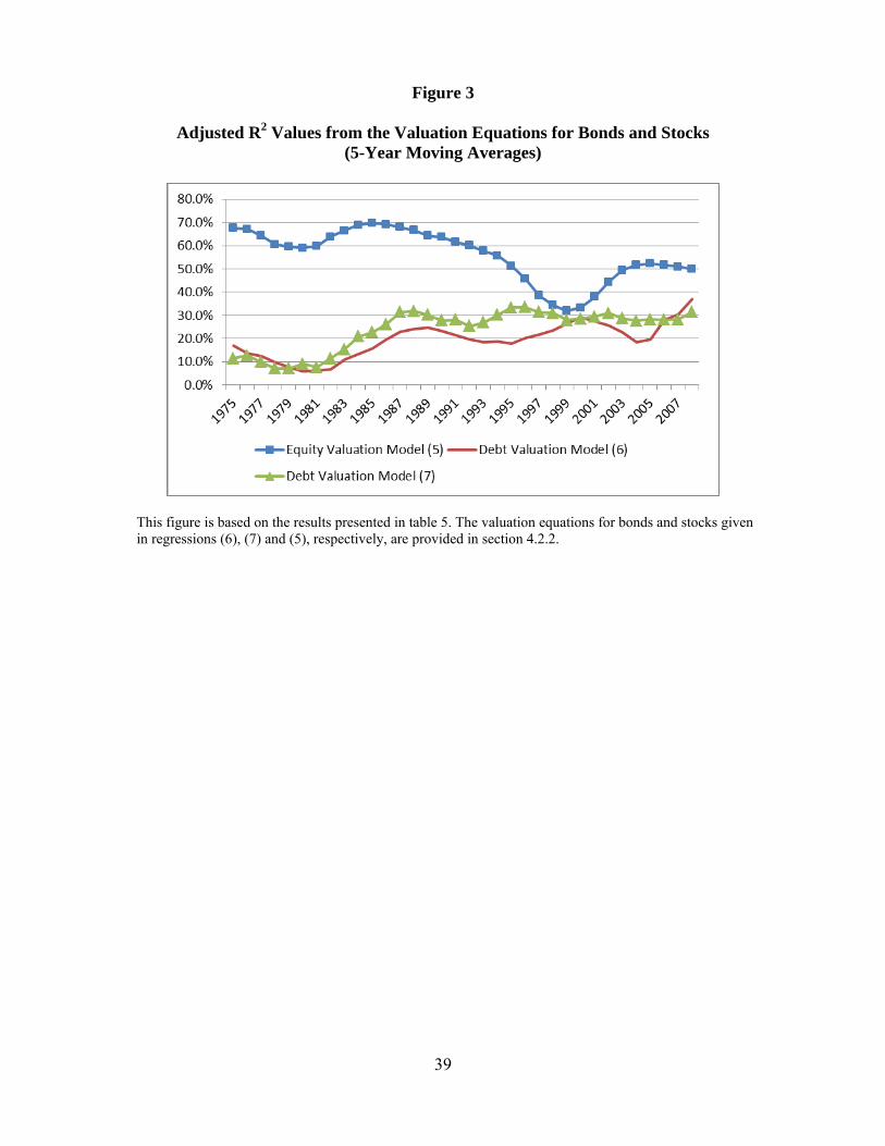
6.2.1. R2 values between market valuation and accounting information. The association
between accounting information and the valuation of bonds and stocks is presented in table 5 and
figure 3. The table shows the adjusted R2 values over time from the valuation equations for
22
bonds and stocks estimated annually. These equations are provided by regressions (6) and (7) for
bonds and by regression (5) for stocks as described in section 4.2.2.13
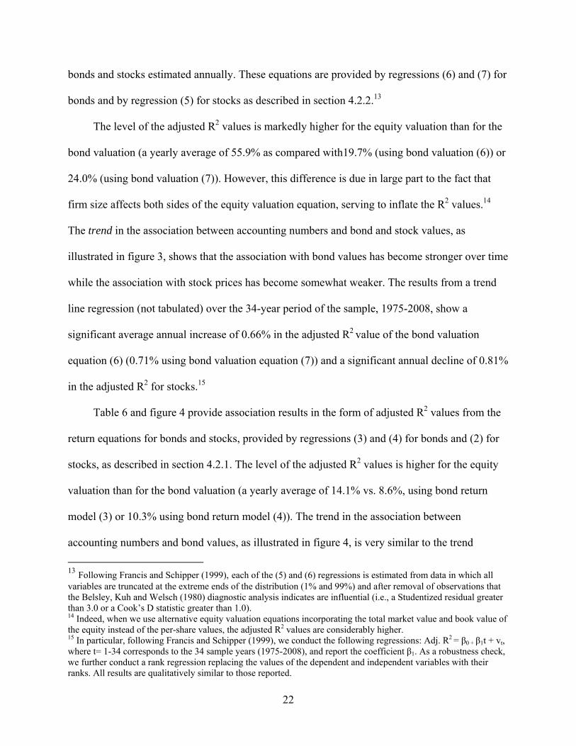
The level of the adjusted R2 values is markedly higher for the equity valuation than for the
bond valuation (a yearly average of 55.9% as compared with19.7% (using bond valuation (6)) or
24.0% (using bond valuation (7)). However, this difference is due in large part to the fact that
firm size affects both sides of the equity valuation equation, serving to inflate the R2 values.14
The trend in the association between accounting numbers and bond and stock values, as
illustrated in figure 3, shows that the association with bond values has become stronger over time
while the association with stock prices has become somewhat weaker. The results from a trend
line regression (not tabulated) over the 34-year period of the sample, 1975-2008, show a
significant average annual increase of 0.66% in the adjusted R2 value of the bond valuation
equation (6) (0.71% using bond valuation equation (7)) and a significant annual decline of 0.81%
in the adjusted R2 for stocks.15
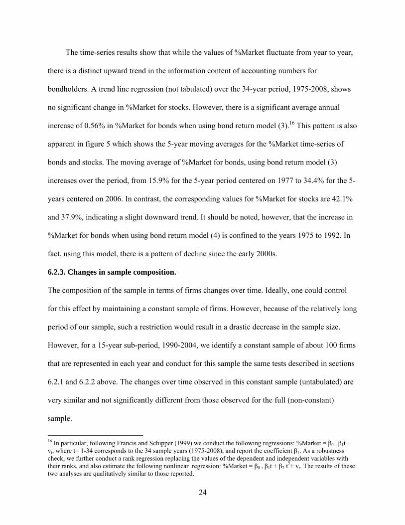
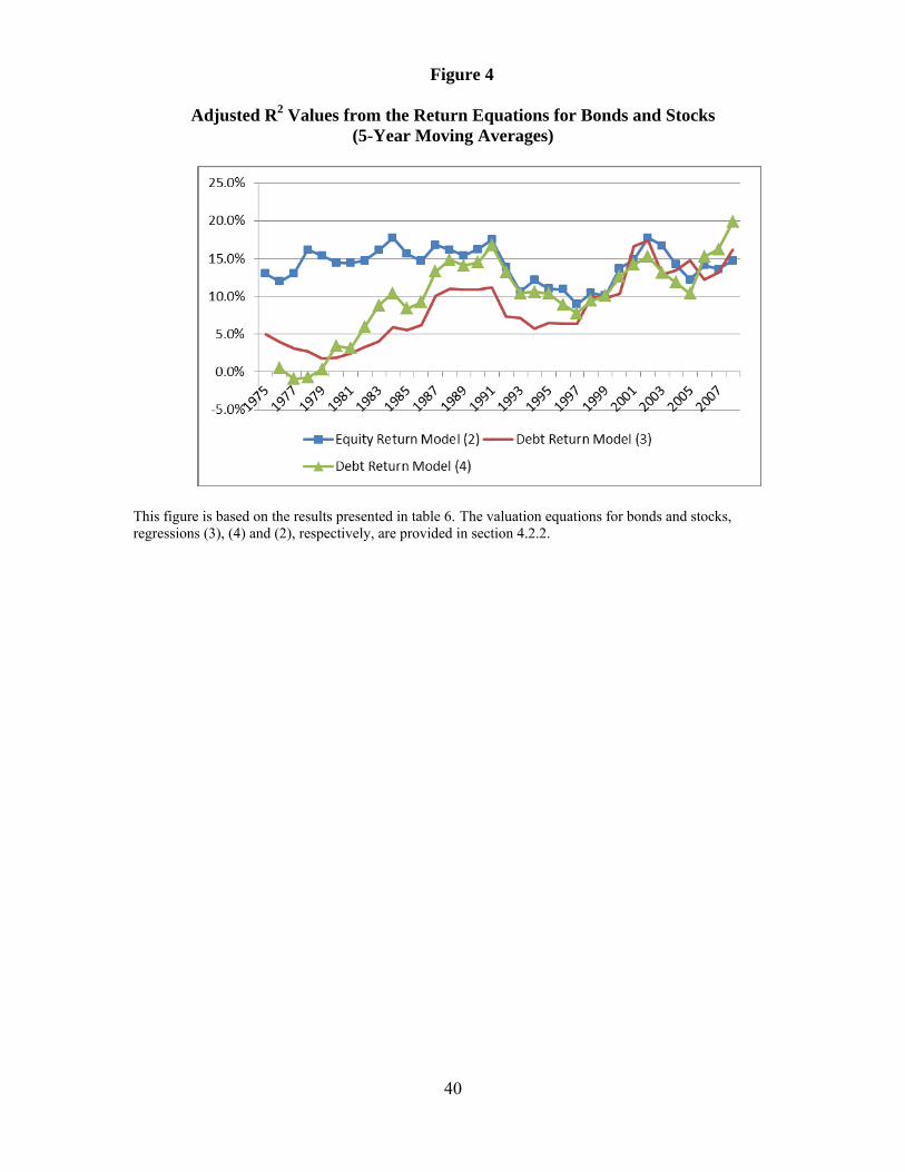
Table 6 and figure 4 provide association results in the form of adjusted R2 values from the
return equations for bonds and stocks, provided by regressions (3) and (4) for bonds and (2) for
stocks, as described in section 4.2.1. The level of the adjusted R2 values is higher for the equity
valuation than for the bond valuation (a yearly average of 14.1% vs. 8.6%, using bond return
model (3) or 10.3% using bond return model (4)). The trend in the association between
accounting numbers and bond values, as illustrated in figure 4, is very similar to the trend
13 Following Francis and Schipper (1999), each of the (5) and (6) regressions is estimated from data in which all variables are truncated at the extreme ends of the distribution (1% and 99%) and after removal of observations that the Belsley, Kuh and Welsch (1980) diagnostic analysis indicates are influential (i.e., a Studentized residual greater than 3.0 or a Cook’s D statistic greater than 1.0). 14 Indeed, when we use alternative equity valuation equations incorporating the total market value and book value of the equity instead of the per-share values, the adjusted R2 values are considerably higher. 15 In particular, following Francis and Schipper (1999), we conduct the following regressions: Adj. R2 = β0 + β1t + vt, where t= 1-34 corresponds to the 34 sample years (1975-2008), and report the coefficient β1. As a robustness check, we further conduct a rank regression replacing the values of the dependent and independent variables with their ranks. All results are qualitatively similar to those reported.

23
exhibited for the valuation equation shown in figure 3. Specifically, the association between
accounting information and bond values has become stronger over time. The results from a trend
line regression (not tabulated) over the 34-year period, 1975-2008, show a significant average
annual increase of 0.40% in the adjusted R2 value of the bond return equation for bond return
model (3)) and an average annual increase of 0.48% using bond return model (4), yet no
significant change in the adjusted R2 values for stocks.
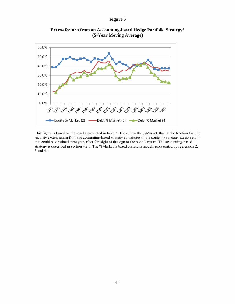
6.2.2. Return from an accounting-based hedged portfolio strategy. The excess returns from a
strategy based on having perfect knowledge of accounting information and the fraction of this
excess return gained from a strategy based on having foreknowledge of the sign of the excess
return, denoted %Market, are presented in table 7 and figure 5. The results are based on a
sample of firms that have the required data for both bonds and stocks.
In general, stock returns appear to be more affected by accounting information than bond
returns. When computed over the pooled sample of firm-years, the mean excess return from an
accounting-based strategy is 14.4% for stocks and only 4.0% for bonds based on regression (3)
and 3.3% based on regression (4) (see the second line of the table). This finding is undoubtedly
due to the greater variability of stock prices as compared with bond prices. More telling about
the role of accounting information in these two markets is that these excess returns represent a
higher %Market (i.e., a higher fraction of the excess return that could be obtained from having
perfect knowledge of the direction of the security price) for stocks than bonds, 42.7% vs. 37.3%
based on regression (3) and 32.1% based on regression (4). In fact, only in seven of the 34 years
examined do bonds exhibit a higher %Market value than do stocks. These results suggest that
accounting information plays a prominent role in the valuation of both types of securities albeit a
somewhat reduced one in the bond market.
24
The time-series results show that while the values of %Market fluctuate from year to year,
there is a distinct upward trend in the information content of accounting numbers for
bondholders. A trend line regression (not tabulated) over the 34-year period, 1975-2008, shows
no significant change in %Market for stocks. However, there is a significant average annual
increase of 0.56% in %Market for bonds when using bond return model (3).16 This pattern is also
apparent in figure 5 which shows the 5-year moving averages for the %Market time-series of
bonds and stocks. The moving average of %Market for bonds, using bond return model (3)
increases over the period, from 15.9% for the 5-year period centered on 1977 to 34.4% for the 5-
years centered on 2006. In contrast, the corresponding values for %Market for stocks are 42.1%
and 37.9%, indicating a slight downward trend. It should be noted, however, that the increase in
%Market for bonds when using bond return model (4) is confined to the years 1975 to 1992. In
fact, using this model, there is a pattern of decline since the early 2000s.
6.2.3. Changes in sample composition.
The composition of the sample in terms of firms changes over time. Ideally, one could control
for this effect by maintaining a constant sample of firms. However, because of the relatively long
period of our sample, such a restriction would result in a drastic decrease in the sample size.
However, for a 15-year sub-period, 1990-2004, we identify a constant sample of about 100 firms
that are represented in each year and conduct for this sample the same tests described in sections
6.2.1 and 6.2.2 above. The changes over time observed in this constant sample (untabulated) are
very similar and not significantly different from those observed for the full (non-constant)
sample.
16 In particular, following Francis and Schipper (1999) we conduct the following regressions: %Market = β0 + β1t + vt, where t= 1-34 corresponds to the 34 sample years (1975-2008), and report the coefficient β1. As a robustness check, we further conduct a rank regression replacing the values of the dependent and independent variables with their ranks, and also estimate the following nonlinear regression: %Market = β0 + β1t + β2 t
2+ vt. The results of these two analyses are qualitatively similar to those reported.
25
6.2.4. Predictive power of accounting information with respect to rating downgrades. The
results concerning the change over time in the predictive ability of accounting numbers with
respect to future rating downgrades, our third measure of information content, are provided in
table 8 and figure 6. As explained in section 4.2.4, given the scarcity of rated bonds in our
sample, we define “downgraded” bonds each year as those in the bottom decile of the
distribution of bond excess returns in that year.17
The table provides values of Somers’ D statistic (Somers, 1962) which is a measure of
association that captures the predictive power of the model with respect to downgrades.18 While
the D statistics fluctuate from year to year, there is an upward trend over time which is also
evident in figure 6. The trend is statistically significant when estimated from a non-linear trend
function (see footnote 16 for the specification of this trend function).
6.2.5. Source of the increased information content of accounting numbers for bondholders.
To explore the causes of the increase over time in the information content of accounting numbers
for bondholders, we first conduct a univariate analysis in which we examine the association
between the variation over time of that content and each of the factors that have been shown to
affect its cross-sectional variation, namely, the yield spread, the frequency of losses and the
frequency of earning declines (see section 6.1 and table 4).
An additional factor that may affect the information content of accounting numbers to
bondholders is the extent of conservatism inherent in these numbers. The potentially important
17 We also use an alternative definition of “downgraded” bond, those in the bottom quartile of the distribution of bond excess returns for the year. This definition, which obviously resulted in a larger number of “downgrades,” produces results that are very similar to those using the original definition. 18 The Somers’ D statistic is closely related to the Kendall’ tau rank correlation coefficient. It is calculated as (Nc–Nd)/N, where N is the total number of paired observations with opposing outcomes in the sample (downgrade versus no downgrade), Nc is the number of pairs in which the model’s estimated likelihood of a downgrade for the realized downgrade member of the pair is higher than that probability for the member of the pair without a downgrade (a “concordant” pair), and Nd is the number of pairs in which the model’s estimated likelihood of a downgrade for the realized downgrade member of the pair is lower than that probability for the member of the pair with no downgrade (a “discordant” pair).
26
role played by conservative accounting in facilitating debt contracting and hence debt valuation
is well recognized by the literature (e.g., Watts and Zimmerman 1986; Ball 2001; Watts 2003a,
b). A number of papers examine efficiency gains from accounting conservatism in debt contracts
(e.g., Ahmed et al. 2002; Zhang 2008; Ball et al. 2008a, b; Beatty et al. 2008; Wittenberg-
Moerman 2008;Vasvari 2006), suggesting a link between conservative reporting and the
information content of accounting numbers for debt holders.
To better separate the economic factors from the reporting causes of the upward trend in
the information content of accounting numbers to bondholders, we also examine the behavior
over time of another economic measure, percentage of cases with negative cash flows from
operations (CFO) which, unlike the percentage of losses, is less likely to be influenced by
accounting conservatism.19
The main measure of conservatism that we use captures the relative persistence of losses
and gains. This measure, suggested by Ball and Shivakumar (2005), is estimated as coefficient
3 from the following piecewise linear regression:
NIi,t = 0 + 1DNIi, t-1 + 2NIi, t-1 + 3DNIi, t-1*NIi, t-1 + i, t (9)
where NI is the change in income excluding extraordinary items from fiscal year t-1 to t, scaled
by the beginning book value of total assets and DNI is a dummy variable set equal to one if
NI in the prior year is negative and zero otherwise. To obtain a less noisy estimate of the trend
in conservatism over time, regression (9) is estimated each year (t=0) from firm-years pooled
over moving, overlapping 5-year intervals beginning two years prior to the observation year (i.e.,
years t-2 to t+2). This measure, which has been employed by a number of studies (e.g., Ball and
19 The frequency of losses and earnings declines could mirror the effect of both economic factors (such as greater business uncertainty or greater competition) and reporting factors. In particular, accounting conservatism in the form of a more timely recognition of losses has been shown to affect earnings variability and skewness (see Givoly and Hayn 2000), properties that induce losses and earnings declines.
27
Shivakumar 2005; Katz 2009; Givoly et al. 2010), relies on the notion that deferring the
recognition of gains until their related cash flows are realized causes gains to be a “persistent”
positive component of accounting income that tends not to reverse. The hypothesis that
economic losses are recognized in a more timely fashion than gains implies that 3 < 0.20
The time-series behavior of these variables is depicted in figure 7a and 7b. Figure 7a
shows the behavior over time of the factors presumed to affect the information content of
accounting numbers to bondholders and figure 7b depicts the corresponding trend over time for
several of our measures of information content. As the figures show, both the factors affecting
that information content (represented by the yield spread, percentage of earning declines,
percentage of losses, percentage of negative cash flows, and accounting conservatism captured
by the reversed-signed value of the coefficient 3 from regression (9)) and the measures of
information content to bondholders (the adjusted R2 values from the bond return regression (3)
and valuation regression (4), as well as %Market based on regression (3)) are all increasing over
time. This positive association is quite strong and, for the most part, statistically significant. For
example, the Spearman correlation coefficients between the annual values of R2 from the return
regression (3) on one hand and the annual yield spread, percentage of losses, percentage of
earnings declines, and percentage of negative CFO cases on the other hand (not tabulated), are
0.428 (1.2% significance level), 0.436 (1.0% significance level), 0.297 (8.8% significance level),
and 0.368 (3.2% significance level). The correlation coefficients of these four factors and the
information content to bondholders measured by %Market rather than by the adjusted R2 values
are 0.316 (6.9% significance level),0.570 (0.04% significance level), 0.487 (0.4% significance
level), and 0.504 (0.2% significance level). We further observe a positive correlation over time
20 Estimating regression (9) using a measure of NI that includes extraordinary items produces similar results.
28
between the degree of conservatism and the information content measures. For example, the
Spearman correlation coefficient between conservatism and the annual values of R2 from the
return regression (3) and %Market are 0.452 (1.4% significance level) and 0.288 (13.0%
significance level), respectively.
The implications of the above results for accounting standard setting depend on whether
the documented increase over time in the information content is caused primarily by changes in
economic factors or changes in the reporting regime. To separate between the effects of reporting
and economic factors on the change over time in the information content of accounting numbers
for bondholders, we next conduct a multivariate test in which we estimate the following
regression of an index of the information content measures considered by the study
(INFO_Index) on the economic and reporting factors described above that are presumed to affect
this content. Specifically, we estimate the following time-series regression of the annual
observations:
INFO_Indext = β0+ β1(YSpread)t + β2(Loss)t + β3(Neg CFO)t +
β4Conservatismt-1 +υt (10)
where INFO_Indext is a composite measure of information content as described below and
YSpreadt is the mean yield spread (or the “excess” yield) at the end of year t computed across all
bonds. The yield spread is measured as the difference between the yield-to-maturity on the bond
and yield-to-maturity of a matched Treasury note as described in section 4.1. Losst and NegCFOt
are the percentage of firms with, respectively, negative earnings and a negative cash flows from
operations at the end of year t. Conservatismt-1 is an estimate of the firm-year conservatism
measure (i.e., the negative of the signed value of coefficient 3 in regression (9)). We use the
29
lagged value of Conservatism since the level of conservatism for the current year is unobservable
to investors.21
INFO_Index for each year is obtained by ranking the individual years by each of the
three cross-sectional measures of information content, namely, the adjusted R2 from the
valuation regression (6), the adjusted R2 from the return regression (3), and %Market from the
return regression (3).22 We then divide the years into deciles according to the distribution of the
34 yearly values of the measure, with the years with the highest (lowest) value of the measure
assigned to decile 9 (0). The value of INFO_Index for year t is obtained by summing the ranks of
the three measures for that year and dividing it by 27 so that the standardized range lies between
0 and 1.
To exploit the full information contained in the individual firm-years, we also estimate a
regression similar to (10) from the sample of firm-year observations pooled over years as
follows:
DRj,t = β0 + β1(YSpread)j,t + β2SignEj,t + β3SignCFOj,t + β4 C* Score j,t-1 + υ j,t (11)
where DRj,t is a measure of the information content for individual firm j in year t. DR, which is
similar in spirit to the cross-sectional measure %Market, is a dummy variable that equals 1 if the
return from an investment strategy based on perfect foresight of accounting numbers (as
described in section 4.2.3) has the same sign as the realized return and 0 otherwise. Yspread j,t is
the yield spread as defined earlier. SignEj,t and SignCFOj,t are dummy variables that receive the
21 Strictly speaking, the other determinants of the information content of accounting numbers for bondholders, namely the current year’s yield spread and the current year’s signs of earnings and cash flows are also unknown in the current year. However, these parameters can be fairly reliably assessed by investors through interim reports and other publicly available information. 22 The results are qualitatively similar if an index based on the adjusted R2 from the valuation regression (7), and the adjusted R2 and %Market from the return regression (4) are used.
30
value of 1 if, respectively, net income and cash flows from operations is negative and 0
otherwise.
To obtain the firm-year estimate of 3, we follow the approach used by Khan and Watts
(2009) to estimate a “C score,” the firm-year estimate of Basu’s (1997) main measure of
conservatism. Specifically, we augment regression (9) with interaction terms between the
independent variables and a linear function of the firm’s attributes that are likely to affect the
relative timeliness of reporting good versus bad news. These attributes are the firm’s size, its
market-to-book ratio and leverage. Specifically, we estimate the following annual cross-sectional
regression:
NIi,t = β1
+ β2DNIi,t-1
+ NIi,t-1(μ1
+ μ2Sizei,t+ μ3M/Bi,t
+ μ
4Levi,t) +
DNIi, t-1*NIi,t-1(δ1 + δ2Sizei,t
+ δ3M/Bi,t+ δ4Levi,t) +
(λ1Sizei,t + λ2M/Bi,t
+ λ3Levi,t
+ λ4DNIi, t-1Sizei,t
+
λ5DNIi,t-1M/Bi,t + λ6DNIi, t-1Levi,t) + εi,t (12)
The estimates obtained from the augmented regression (12) are then used to estimate a
“modified” C Score which we denote as C* Score for each firm year as a linear function of firm-
specific characteristics as follows:
C*Score (the firm-yeari,t α3) = δ1,t + δ2,tSIZEi,t + δ3,tM/Bi,t + δ4,tLevi,t (13)
where this linear function is estimated from regression (12) in which it serves as the coefficient
of DNI j, t-1*NIi,t-1.23 For ease of interpretation, in regression (11) we use the flipped sign of
the estimated C* Score, multiplying the actual estimate by negative one.
The results from regressions (10) and (11) are presented in tables 9 and 10, respectively.
Table 9 shows that the strong and significance associations between the composite measure of
information content and firm-specific factors that are hypothesized to affect it are weakened or
23 See section 2.2 of Khan and Watts (2005) for details of the derivation.

31
eliminated in a multivariate setting. In particular, the percentage of losses is no longer a
significant explanatory variable once we introduce either the % of negative cash flows variable
or conservatism. This finding reinforces the notion that the percentage of losses is a reflection of
both economic factors (captured by the behavior of cash flows) and reporting factors (captured
by conservatism).
Two factors that are significant throughout the multivariate tests are the yield spread and
conservatism. In the regression with the full set of variables (reported in the last column of the
table), the yield spread has a positive coefficient (t-statistic of 3.17) and conservatism has a
positive coefficient (t-statistic of 2.61).
Table 10 shows the results from estimating regression (11). As explained above, this
regression is estimated from individual firm-years with the dependent variable being a measure
of information content based on a variation of the %Market construct. The results from this
regression are somewhat different from those obtained from regression (10). In particular, the
occurrence of negative cash flows from operations becomes significant (t-statistic of 1.75) and
the occurrence of a loss replaces conservatism as the second significant variable in addition to
yield spread. Conservatism continues to be positively related to the information content and it
borders on being significant at the 10% level (two-sided). Note, however, the limitations of the
findings based on this regression relative to those based on regression (10). First, the measure of
information content is based on a single measure (a variation of %Market) rather than the
composite measure used in regression (10). Second, the conservatism measure used in regression
(11), the “modified” C*Score, is based on a series of estimates and assumptions, a likely source
of additional measurement error. 24
24 For example, the assumptions regarding the factors affecting conservatism and their linear and cross-sectionally constant relationship with conservatism may not hold in all situations.

32
7. Concluding Remarks
This paper provides large-sample evidence on the role that accounting information plays
in bond valuation. The findings indicate that both the valuation of bonds and their returns are
more sensitive to adverse accounting information and more responsive to accounting information
in situations in which the likelihood of default is higher. Using several approaches for capturing
and measuring the “information content,” the results show that the information content of
accounting information from the debt holders’ perspective has increased over the last 34 years.
This is in contrast to the information content of accounting numbers for shareholders which, as
has been documented by past research and further confirmed on this sample, has stayed at the
same level or even declined slightly.
The paper also finds that the increase in accounting conservatism (previously documented
by Basu 1997 and Givoly and Hayn 2002 and reconfirmed by this study) is associated with the
increase in the information content of accounting numbers for bondholders. The results from the
cross-sectional tests, although only marginally significant (possibly because of difficulties in
measuring conservatism for individual firm-years) are also consistent with the notion that
conservatism is positively related to the information content of accounting numbers for
bondholders. The finding of a link between accounting conservatism and the information content
of accounting numbers is yet another demonstration of the economic consequences of
conservatism.
The paper highlights the importance of recognizing the unique information needs of debt
holders, a major group of users of financial statement information, in forming and evaluating the
merits of accounting standards. As such, the findings have implications for accounting standard
setting, regulatory policy and research on the information content of financial reports.

33
References
Ahmed, A., B. Billings, R. Morton, and M. Stanford-Harris, 2002. “The Role of Accounting Conservatism in Mitigating Bondholder-Shareholder Conflicts over Dividend Policy and in Reducing Debt Costs,” The Accounting Review, 77 (4): 867-890. Aboody, D., and B. Lev, 1998. “The Value Relevance of Intangibles: The Case of Software Capitalization,” Journal of Accounting Research, 36: 161-191. Baker, M., R. Greenwood, and J. Wurgler, 2003. “The Maturity of Debt Issues and Predictable Variation in Bond Returns,” Journal of Financial Economics, 70: 261-291. Ball, R., 2001. “Infrastructure Requirements for an Economically Efficient System of Public Financial Reporting and Disclosure,” Brookings-Wharton Papers on Financial Services, pp.127–169. Ball, R., R.M. Bushman, and F.P. Vasvari, 2008a. “The Debt-Contracting Value of Accounting Information and Loan Syndicate Structure,” Journal of Accounting Research, 46 (2): 247-287. Ball, R., A. Robin, and G. Sadka, 2008b. “Is Financial Reporting Shaped by Equity markets or by Debt Markets” An International Study of Timeliness and Conservatism,” The Review of Accounting Studies, 13 (2-3): 168-205. Ball, R., and L. Shivakumar, 2005. “Earnings Quality in UK Private Firms: Comparative Loss Recognition Timeliness,” Journal of Accounting and Economics, 39 (1): 83–128. Basu, S., 1997. “The Conservatism Principle and Asymmetric Timeliness of Earnings,” Journal of Accounting and Economics 24 (1): 3–37. Beatty, A.L., J.P. Weber, and J.J. Yu, 2008. “Conservatism and Debt,” Journal of Accounting and Economics 48 (2-3): 154-174. Belsley, D., E. Kuh, and R. Welsch. Regression Diagnostics. New York: Wiley, 1980. Burgstahler, D., and I. Dichev. 1997. “Earnings Management to Avoid Earnings Decreases and Losses.” Journal of Accounting and Economics, 24 (1): 99–126. Collins, D., E. Maydew, and I. Weiss, 1997. “Change in the Value-relevance of Earnings and Book Values over the Past Forty Years,” Journal of Accounting & Economics 34: 43-64. Cooper, R. A., and J.M. Shulman, 1994. “The Year-End Effect in Junk Bond Prices,” Financial Analysts Journal, Sep/Oct, 50 (5): 61-65. Datta, S., and U.S. Dhillon, 1993. “Bond and Stock Market Response to Unexpected Earnings Announcements,” The Journal of Financial and Quantitative Analysis 28 (4): 565-577.
34
Davis, D. W., J. R. Boatsman, and E. F. Baskin, 1978. “On Generalizing Stock Market Research to a Broader Class of Markets,” The Accounting Review,53 (1): 1-10. DeFond, M., and J. Zhang, 2009. “The Asymmetric Magnitude and Timeliness of the Bond Market Reaction to Quarterly Earnings Announcements,” Working Paper, University of Southern California. DeFond, M., and J. Zhang,, 2011. “The Timeliness of the Bond Market Reaction to Bad News Earnings Surprises,” Working Paper, University of Southern California. Dou, Y., 2013. “The Debt-Contracting Value of Accounting Numbers, Renegotiation, and Investment Efficiency,” Working Paper, New York University. Dudney, D., and J. Geppert, 2008. “Do Tax-Exempt Yields Adjust Slowly to Substantial Changes in Taxable Yields?” Journal of Futures Markets, 28 (8): 763-789 Easton, P. D., S, J. Monhahn, and F. P. Vavai, 2009. “Initial Evidence on the Role of Accounting Earnings in the Bond Market,” Journal of Accounting Research, 47 (3): 721- 766. Elliott, J.A., A. Ghosh, and D. Moon, 2010. “Asymmetric Valuation of Sustained Growth by Bond- and Equity-holders,” Review of Accounting Studies, 15: 833-878. Ely, K., and G. Waymire, 1999. “Accounting Standard-setting Organizations and Earnings Relevance: Longitudinal Evidence from NYSE Common Stock, 1927-93,” Journal of Accounting Research, 37: 293-318. Fischer, P.E., and R.E. Verrecchia, 1997. “The Effect of Limited Liability on the Market Response to Disclosure,” Contemporary Accounting Research, 14 (3): 515-541. Francis J., and K. Schipper, 1999. “Have Financial Statements Lost their Relevance?” Journal of Accounting Research, 37: 319-352. Gay, G. D., and S. Manaster, 1991. “Equilibrium Treasury Bond Futures Pricing in the Presence of Implicit Delivery Options,” Journal of Futures Markets, 11 (5): 623-645. Givoly, D., and C. Hayn, 2000. “The Changing Time-Sseries Properties of Earnings, Cash Flows and Accruals: Has Financial Reporting Become More Conservative?,” Journal of Accounting and Economics 29: 287–320. Givoly, D., C. Hayn, and S. Katz, 2010. “Does Public Ownership of Equity Improve Earnings Quality?,” The Accounting Review, 85 (1): 195-225. Gkougkousi, X., 2012. “Aggregate Earnings and Corporate Bond Markets,” Working Paper, Erasmus University.
35
Hancock, D., and M.L. Kwast, 2001. “Using Subordinated Debt to Monitor Bank Holding Companies: Is it Feasible?” Journal of Financial Services Research, 20 (2/3): 147-187. Hand, J. R.M., R.W. Holthausen, and R.W. Leftwich, 1992. “The Effect of Bond Rating Agency Announcements on Bond and Stock Prices,” The Journal of Finance, 47 (2): 733-752. Hayn, C., 1995. “The Information Content of Losses.” Journal of Accounting and Economics, 20: 125-153. Hemler, M. L., 1990. “The Quality Delivery Option in Treasury Bond Futures Contracts,” Journal of Finance, 45 (5): 1565-1586. Katz, S., 2009. “Earnings Quality and Ownership Structure: The Role of Private Equity Sponsors,” The Accounting Review 84 (3): 623–658. Khan, M., and R. Watts, 2009. “Estimation and Empirical Properties of a Firm-Year Measure of Accounting Conservatism,” Journal of Accounting and Economics, 48: 132-150. Khurana, I., and K. Raman, 2003. “Are Fundamentals Priced in the Bond Market?,” Contemporary Accounting Research, 20 (3): 465-494. Klein A., and E. Zur, 2011. “The Impact of Hedge Fund Activism on the Target Firm’s Existing Bondholders,” Review of Financial Studies, 22: 1735-1771. Lev, B., and T. Sougiannis, 1996.”The Capitalization, Amortization and Value Relevance of R&D,” Journal of Accounting and Economics, 21: 107-138. Lev, B., and P. Zarowin, 1999. “The Boundaries of Financial Reporting and How to Extend Them,” Journal of Accounting Research, 37: 354-385. Plummer, E. C., and S. Y. Tse, 1999. “The Effect of Limited Liability on the Informativeness of Earnings: Evidence from the Stock and Bond Markets,” Contemporary Accounting Research, 16 (3): 541-574. Ramesh, K., and R. Thiagarajan, 1996. “Inter-temporal Decline in Earnings Response Bondholders’ Perspective,” Journal of Accounting and Economics, 35 (2): 227-254. Shi, C. 2003. “On the Trade-off Between the Future Benefits and Riskiness of R&D: A Bondholders’ Perspective.” Journal of Accounting and Economics 35 (2): pp. 227-254. Shulman, J., and M. Bayless, 1993. “Marketability and Default Influences on the Yield Premia of Speculative-Grade Debt,” The Journal of the Financial Management Association, 22 (3): 132-141. Sridharan, S. A., 2011. “The Valuation Role of the Balance Sheet Information in the Corporate Bond Market,” Working Paper, Stanford University.
36
Somers, R.H., 1962. “A New Asymmetric Measure of Association for Ordinal Variables,” American Sociological Review, 27 (6): 799-811. Vasvari, F., 2006, “Managerial Incentive Structures, Conservatism and the Pricing of syndicated loans,” Working Paper, London Business School.
Watts, R., 2003a. “Conservatism in Accounting, Part I: Explanations and Implications,” Accounting Horizons, 17: 207–21. Watts, R., 2003b. “Conservatism in Accounting, Part II: Evidence and Research Opportunities,” Accounting Horizons, 17: 287–301. Watts, R., and J. Zimmerman. 1986. Positive Accounting Theory. Englewood Cliffs, NJ: Prentice-Hall Inc. Whittenberg-Noerman, R., 2008. “The Role of Information Asymmetry and Financial Reporting Quality in Debt Contracting: Evidence from the Secondary Loan Market,” Journal of Accounting and Economics, 46 (2-3): 240-260. Zhang, J., 2008. “The Contracting Benefits of Accounting Conservatism to Lenders and Borrowers,” Journal of Accounting and Economics, 45: 27-54.
37
Figure 1
Association between the Firm’s Operating Performance and Equity Value
Source: Hayn (1995, page 133).
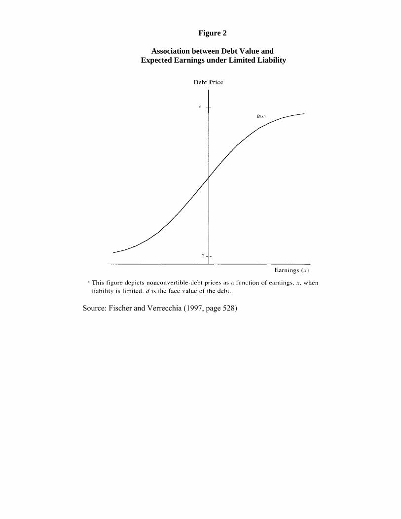
Figure 2
Association between Debt Value and Expected Earnings under Limited Liability
Source: Fischer and Verrecchia (1997, page 528)
39
Figure 3
Adjusted R2 Values from the Valuation Equations for Bonds and Stocks
(5-Year Moving Averages)
This figure is based on the results presented in table 5. The valuation equations for bonds and stocks given in regressions (6), (7) and (5), respectively, are provided in section 4.2.2.
40
Figure 4
Adjusted R2 Values from the Return Equations for Bonds and Stocks (5-Year Moving Averages)
This figure is based on the results presented in table 6. The valuation equations for bonds and stocks, regressions (3), (4) and (2), respectively, are provided in section 4.2.2.
41
Figure 5
Excess Return from an Accounting-based Hedge Portfolio Strategy* (5-Year Moving Average)
This figure is based on the results presented in table 7. They show the %Market, that is, the fraction that the security excess return from the accounting-based strategy constitutes of the contemporaneous excess return that could be obtained through perfect foresight of the sign of the bond’s return. The accounting-based strategy is described in section 4.2.3. The %Market is based on return models represented by regression 2, 3 and 4.
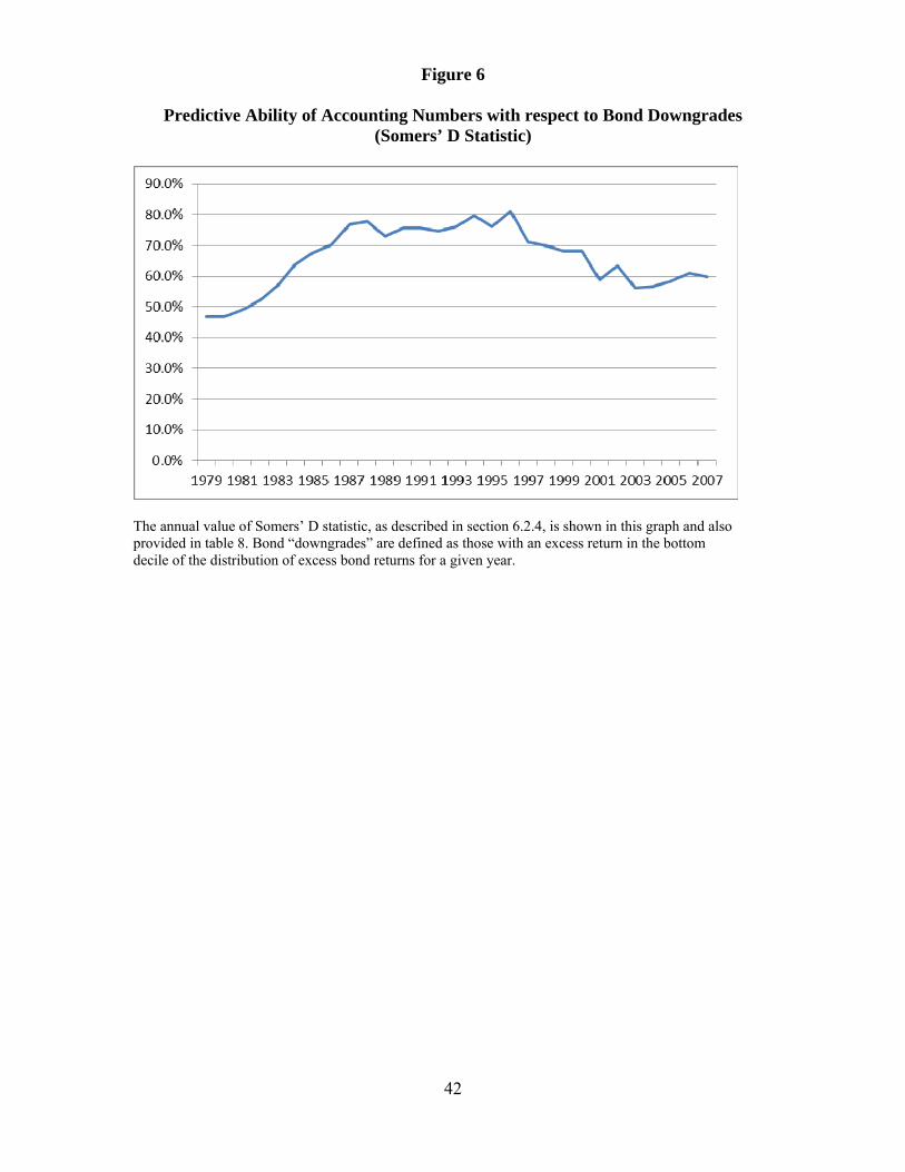
42
Figure 6
Predictive Ability of Accounting Numbers with respect to Bond Downgrades (Somers’ D Statistic)
The annual value of Somers’ D statistic, as described in section 6.2.4, is shown in this graph and also provided in table 8. Bond “downgrades” are defined as those with an excess return in the bottom decile of the distribution of excess bond returns for a given year.
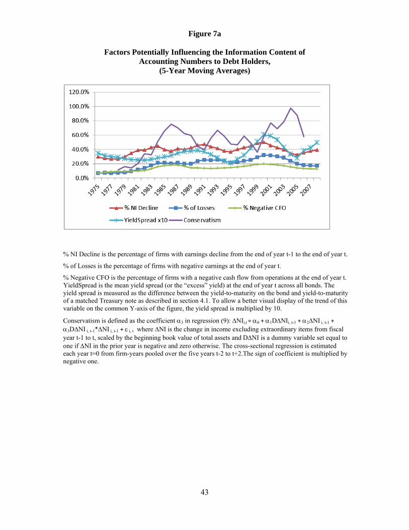
43
Figure 7a
Factors Potentially Influencing the Information Content of Accounting Numbers to Debt Holders,
(5-Year Moving Averages)
% NI Decline is the percentage of firms with earnings decline from the end of year t-1 to the end of year t.
% of Losses is the percentage of firms with negative earnings at the end of year t.
% Negative CFO is the percentage of firms with a negative cash flow from operations at the end of year t. YieldSpread is the mean yield spread (or the “excess” yield) at the end of year t across all bonds. The yield spread is measured as the difference between the yield-to-maturity on the bond and yield-to-maturity of a matched Treasury note as described in section 4.1. To allow a better visual display of the trend of this variable on the common Y-axis of the figure, the yield spread is multiplied by 10.
Conservatism is defined as the coefficient 3 in regression (9): NIi,t = 0 + 1DNIi, t-1 + 2NI i, t-1 +
3DNI i, t-1*NI i, t-1 + i, t where NI is the change in income excluding extraordinary items from fiscal year t-1 to t, scaled by the beginning book value of total assets and DNI is a dummy variable set equal to one if NI in the prior year is negative and zero otherwise. The cross-sectional regression is estimated each year t=0 from firm-years pooled over the five years t-2 to t+2.The sign of coefficient is multiplied by negative one.
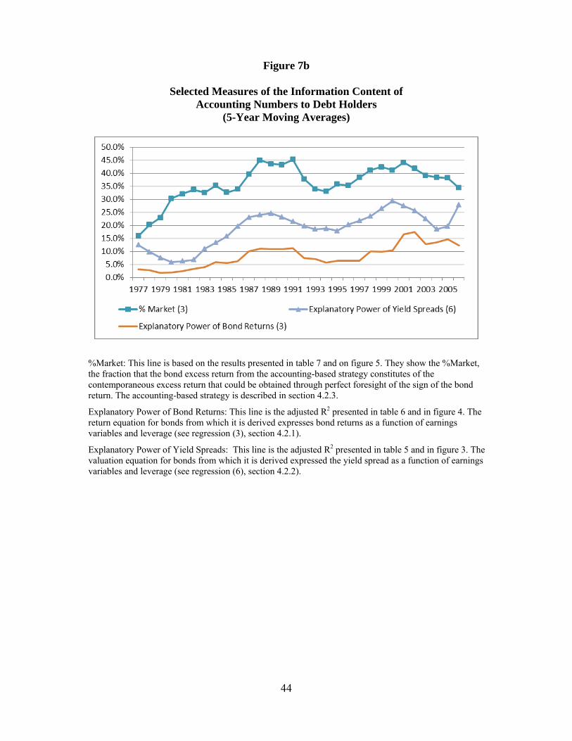
44
Figure 7b
Selected Measures of the Information Content of
Accounting Numbers to Debt Holders (5-Year Moving Averages)
%Market: This line is based on the results presented in table 7 and on figure 5. They show the %Market, the fraction that the bond excess return from the accounting-based strategy constitutes of the contemporaneous excess return that could be obtained through perfect foresight of the sign of the bond return. The accounting-based strategy is described in section 4.2.3.
Explanatory Power of Bond Returns: This line is the adjusted R2 presented in table 6 and in figure 4. The return equation for bonds from which it is derived expresses bond returns as a function of earnings variables and leverage (see regression (3), section 4.2.1).
Explanatory Power of Yield Spreads: This line is the adjusted R2 presented in table 5 and in figure 3. The valuation equation for bonds from which it is derived expressed the yield spread as a function of earnings variables and leverage (see regression (6), section 4.2.2).
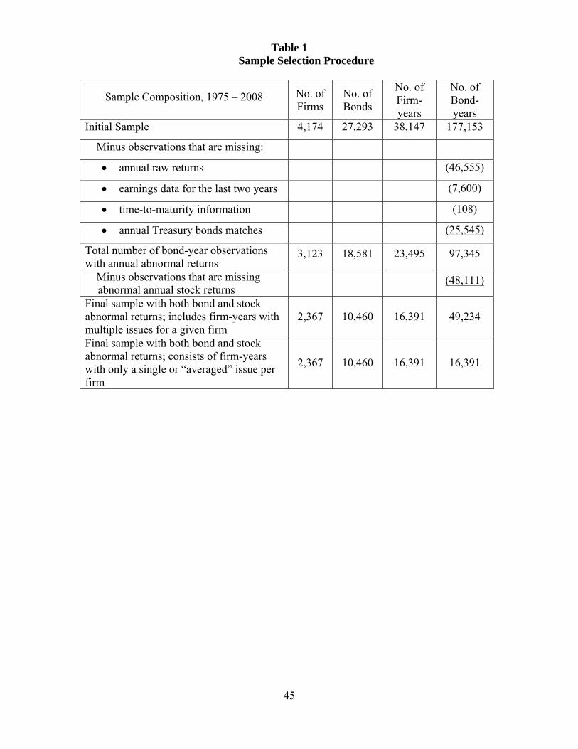
45
Table 1 Sample Selection Procedure
Sample Composition, 1975 – 2008 No. of Firms
No. of Bonds
No. of Firm-years
No. of Bond-years
Initial Sample 4,174 27,293 38,147 177,153
Minus observations that are missing:
annual raw returns (46,555)
earnings data for the last two years (7,600)
time-to-maturity information (108)
annual Treasury bonds matches (25,545)
Total number of bond-year observations with annual abnormal returns
3,123 18,581 23,495 97,345
Minus observations that are missing abnormal annual stock returns
(48,111)
Final sample with both bond and stock abnormal returns; includes firm-years with multiple issues for a given firm
2,367 10,460 16,391 49,234
Final sample with both bond and stock abnormal returns; consists of firm-years with only a single or “averaged” issue per firm
2,367 10,460 16,391 16,391
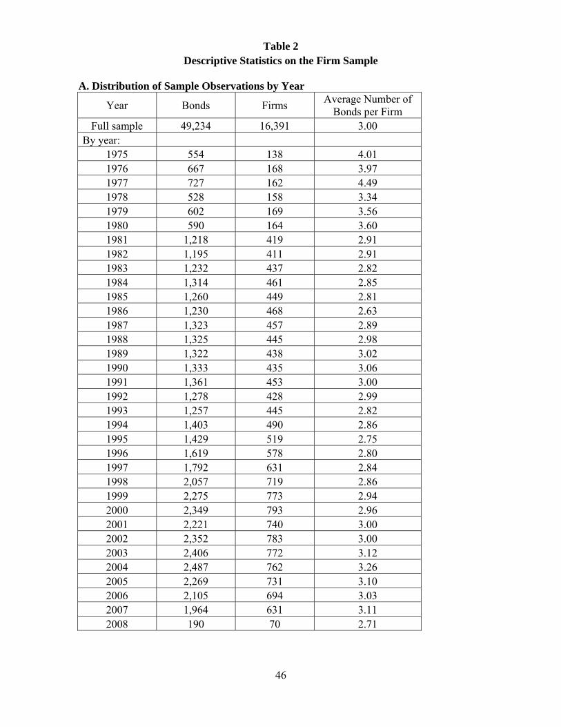
46
Table 2 Descriptive Statistics on the Firm Sample
A. Distribution of Sample Observations by Year
Year Bonds Firms Average Number of
Bonds per Firm Full sample 49,234 16,391 3.00
By year: 1975 554 138 4.01 1976 667 168 3.97 1977 727 162 4.49 1978 528 158 3.34 1979 602 169 3.56 1980 590 164 3.60 1981 1,218 419 2.91 1982 1,195 411 2.91 1983 1,232 437 2.82 1984 1,314 461 2.85 1985 1,260 449 2.81 1986 1,230 468 2.63 1987 1,323 457 2.89 1988 1,325 445 2.98 1989 1,322 438 3.02 1990 1,333 435 3.06 1991 1,361 453 3.00 1992 1,278 428 2.99 1993 1,257 445 2.82 1994 1,403 490 2.86 1995 1,429 519 2.75 1996 1,619 578 2.80 1997 1,792 631 2.84 1998 2,057 719 2.86 1999 2,275 773 2.94 2000 2,349 793 2.96 2001 2,221 740 3.00 2002 2,352 783 3.00 2003 2,406 772 3.12 2004 2,487 762 3.26 2005 2,269 731 3.10 2006 2,105 694 3.03 2007 1,964 631 3.11 2008 190 70 2.71
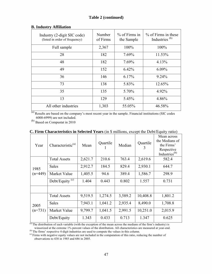
47
Table 2 (continued)
B. Industry Affiliation
Industry (2-digit SIC code) (listed in order of frequency)
Number of Firms
% of Firms in the Sample
% of Firms in these Industries (b)
Full sample 2,367 100% 100%
28 182 7.69% 11.53%
48 182 7.69% 4.13%
49 152 6.42% 6.09%
36 146 6.17% 9.24%
73 138 5.83% 12.65%
35 135 5.70% 4.92%
13 129 5.45% 4.86%
All other industries 1,303 55.05% 46.58% (a) Results are based on the company’s most recent year in the sample. Financial institutions (SIC codes
6000-6999) are not included. (b) Based on Compustat in 2010
C. Firm Characteristics in Selected Years (in $ millions, except the Debt/Equity ratio)
Year Characteristic(a) Mean Quartile
1 Median
Quartile 3
Mean across the Medians of
the Firms’ Respective Industries(b)
1985 (n=449)
Total Assets 2,621.7 210.6 763.4 2,619.6 582.4
Sales 2,912.7 184.5 829.4 2,930.1 644.7
Market Value 1,405.5 94.6 389.4 1,586.7 298.9
Debt/Equity (c) 1.404 0.443 0.802 1.557 0.731
2005 (n=731)
Total Assets 9,519.5 1,274.5 3,589.2 10,408.8 1,801.2
Sales 7,943.1 1,041.2 2,935.4 8,490.0 1,708.8
Market Value 9,799.7 1,041.5 2,991.5 10,251.0 2,015.9
Debt/Equity 1.343 0.433 0.713 1.347 0.625 (a) The distribution of each variable (with the exception of the mean across the medians of the firm’s industry) is
winsorized at the extreme 1% percent values of the distribution. All characteristics are measured at year-end. (b) The firms’ respective 4-digit industries are used to compute the values in this column. (c) Firms with negative equity values are not included in the computation of this ratio, reducing the number of
observations to 438 in 1985 and 686 in 2005.
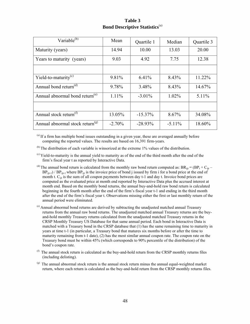
48
Table 3 Bond Descriptive Statistics(a)
Variable(b) Mean Quartile 1 Median Quartile 3
Maturity (years) 14.94 10.00 13.03 20.00
Years to maturity (years) 9.03 4.92 7.75 12.38
Yield-to-maturity(c) 9.81% 6.41% 8.43% 11.22%
Annual bond return(d) 9.78% 3.48% 8.43% 14.67%
Annual abnormal bond return(e) 1.11% -3.01% 1.02% 5.11%
Annual stock return(f) 13.05% -15.37% 8.67% 34.08%
Annual abnormal stock return(g) -2.70% -28.93% -5.11% 18.60%
(a) If a firm has multiple bond issues outstanding in a given year, these are averaged annually before computing the reported values. The results are based on 16,391 firm-years.
(b) The distribution of each variable is winsorized at the extreme 1% values of the distribution. (c) Yield-to-maturity is the annual yield to maturity as of the end of the third month after the end of the
firm’s fiscal year t as reported by Interactive Data. (d) The annual bond return is calculated from the monthly raw bond return computed as: BRijt = (BPt + Cijt –
BPijt-1) / BPijt-1 where BPijt is the invoice price of bond j issued by firm i for a bond price at the end of month t. Cijt is the sum of all coupon payments between day t-1 and day t. Invoice bond prices are computed as the evaluated price at month end reported by Interactive Data plus the accrued interest at month end. Based on the monthly bond returns, the annual buy-and-hold raw bond return is calculated beginning in the fourth month after the end of the firm’s fiscal year t-1 and ending in the third month after the end of the firm’s fiscal year t. Observations missing either the first or last monthly return of the annual period were eliminated.
(e) Annual abnormal bond returns are derived by subtracting the unadjusted matched annual Treasury returns from the annual raw bond returns. The unadjusted matched annual Treasury returns are the buy-and-hold monthly Treasury returns calculated from the unadjusted matched Treasury returns in the CRSP Monthly Treasury US Database for that same annual period. Each bond in Interactive Data is matched with a Treasury bond in the CRSP database that (1) has the same remaining time to maturity in years at time t-1 (in particular, a Treasury bond that matures six months before or after the time to maturity remaining from t-1 date), (2) has the most similar annual coupon rate. The coupon rate on the Treasury bond must be within 45% (which corresponds to 90% percentile of the distribution) of the bond’s coupon rate.
(f) The annual stock return is calculated as the buy-and-hold return from the CRSP monthly returns files (including delisting).
(g) The annual abnormal stock return is the annual stock return minus the annual equal-weighted market return, where each return is calculated as the buy-and-hold return from the CRSP monthly returns files.
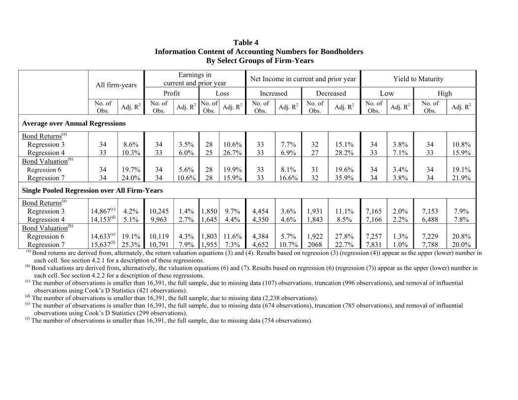
Table 4 Information Content of Accounting Numbers for Bondholders
By Select Groups of Firm-Years
All firm-years
Earnings in current and prior year
Net Income in current and prior year Yield to Maturity
Profit Loss Increased Decreased Low High No. of Obs.
Adj. R2 No. of Obs.
Adj. R2 No. of Obs.
Adj. R2 No. of Obs.
Adj. R2 No. of Obs.
Adj. R2 No. of Obs.
Adj. R2 No. of Obs.
Adj. R2
Average over Annual Regressions
Bond Returns(a)
Regression 3 Regression 4
34 33
8.6% 10.3%
34 33
3.5% 6.0%
28 25
10.6% 26.7%
33 33
7.7% 6.9%
32 27
15.1% 28.2%
34 33
3.8% 7.1%
34 33
10.8% 15.9%
Bond Valuation(b)
Regression 6 Regression 7
34 34
19.7% 24.0%
34 34
5.6% 10.6%
28 28
19.9% 15.9%
33 33
8.1% 16.6%
31 32
19.6% 35.9%
34 34
3.4% 3.8%
34 34
19.1% 21.9%
Single Pooled Regression over All Firm-Years
Bond Returns(a)
Regression 3 Regression 4
14,867(c)
14,153(d) 4.2% 5.1%
10,245 9,963
1.4% 2.7%
1,8501,645
9.7% 4.4%
4,454 4,350
3.6% 4.6%
1,931 1,843
11.1% 8.5%
7,165 7,166
2.0% 2.2%
7,153 6,488
7.9% 7.8%
Bond Valuation(b)
Regression 6 Regression 7
14,633(e)
15,637(f) 19.1% 25.3%
10,119 10,791
4.3% 7.9%
1,8031,955
11.6% 7.3%
4,384 4,652
5.7% 10.7%
1,922 2068
27.8% 22.7%
7,257 7,831
1.3% 1.0%
7,229 7,788
20.8% 20.0%
(a) Bond returns are derived from, alternately, the return valuation equations (3) and (4). Results based on regression (3) (regression (4)) appear as the upper (lower) number in each cell. See section 4.2.1 for a description of these regressions.
(b) Bond valuations are derived from, alternatively, the valuation equations (6) and (7). Results based on regression (6) (regression (7)) appear as the upper (lower) number in each cell. See section 4.2.2 for a description of these regressions.
(c) The number of observations is smaller than 16,391, the full sample, due to missing data (107) observations, truncation (996 observations), and removal of influential observations using Cook’s D Statistics (421 observations).
(d) The number of observations is smaller than 16,391, the full sample, due to missing data (2,238 observations). (e) The number of observations is smaller than 16,391, the full sample, due to missing data (674 observations), truncation (785 observations), and removal of influential
observations using Cook’s D Statistics (299 observations). (f) The number of observations is smaller than 16,391, the full sample, due to missing data (754 observations).
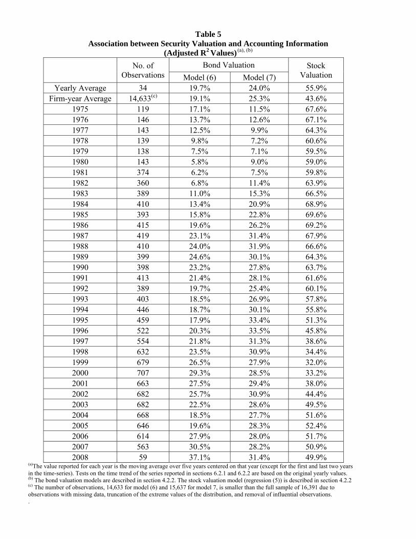
Table 5 Association between Security Valuation and Accounting Information
(Adjusted R2 Values) (a), (b)
No. of
Observations Bond Valuation Stock
Valuation Model (6) Model (7)
Yearly Average 34 19.7% 24.0% 55.9% Firm-year Average 14,633(c) 19.1% 25.3% 43.6%
1975 119 17.1% 11.5% 67.6% 1976 146 13.7% 12.6% 67.1% 1977 143 12.5% 9.9% 64.3% 1978 139 9.8% 7.2% 60.6% 1979 138 7.5% 7.1% 59.5% 1980 143 5.8% 9.0% 59.0% 1981 374 6.2% 7.5% 59.8% 1982 360 6.8% 11.4% 63.9% 1983 389 11.0% 15.3% 66.5% 1984 410 13.4% 20.9% 68.9% 1985 393 15.8% 22.8% 69.6% 1986 415 19.6% 26.2% 69.2% 1987 419 23.1% 31.4% 67.9% 1988 410 24.0% 31.9% 66.6% 1989 399 24.6% 30.1% 64.3% 1990 398 23.2% 27.8% 63.7% 1991 413 21.4% 28.1% 61.6% 1992 389 19.7% 25.4% 60.1% 1993 403 18.5% 26.9% 57.8% 1994 446 18.7% 30.1% 55.8% 1995 459 17.9% 33.4% 51.3% 1996 522 20.3% 33.5% 45.8% 1997 554 21.8% 31.3% 38.6% 1998 632 23.5% 30.9% 34.4% 1999 679 26.5% 27.9% 32.0% 2000 707 29.3% 28.5% 33.2% 2001 663 27.5% 29.4% 38.0% 2002 682 25.7% 30.9% 44.4% 2003 682 22.5% 28.6% 49.5% 2004 668 18.5% 27.7% 51.6% 2005 646 19.6% 28.3% 52.4% 2006 614 27.9% 28.0% 51.7% 2007 563 30.5% 28.2% 50.9% 2008 59 37.1% 31.4% 49.9%
(a)The value reported for each year is the moving average over five years centered on that year (except for the first and last two years in the time-series). Tests on the time trend of the series reported in sections 6.2.1 and 6.2.2 are based on the original yearly values. (b) The bond valuation models are described in section 4.2.2. The stock valuation model (regression (5)) is described in section 4.2.2 (c) The number of observations, 14,633 for model (6) and 15,637 for model 7, is smaller than the full sample of 16,391 due to observations with missing data, truncation of the extreme values of the distribution, and removal of influential observations. .
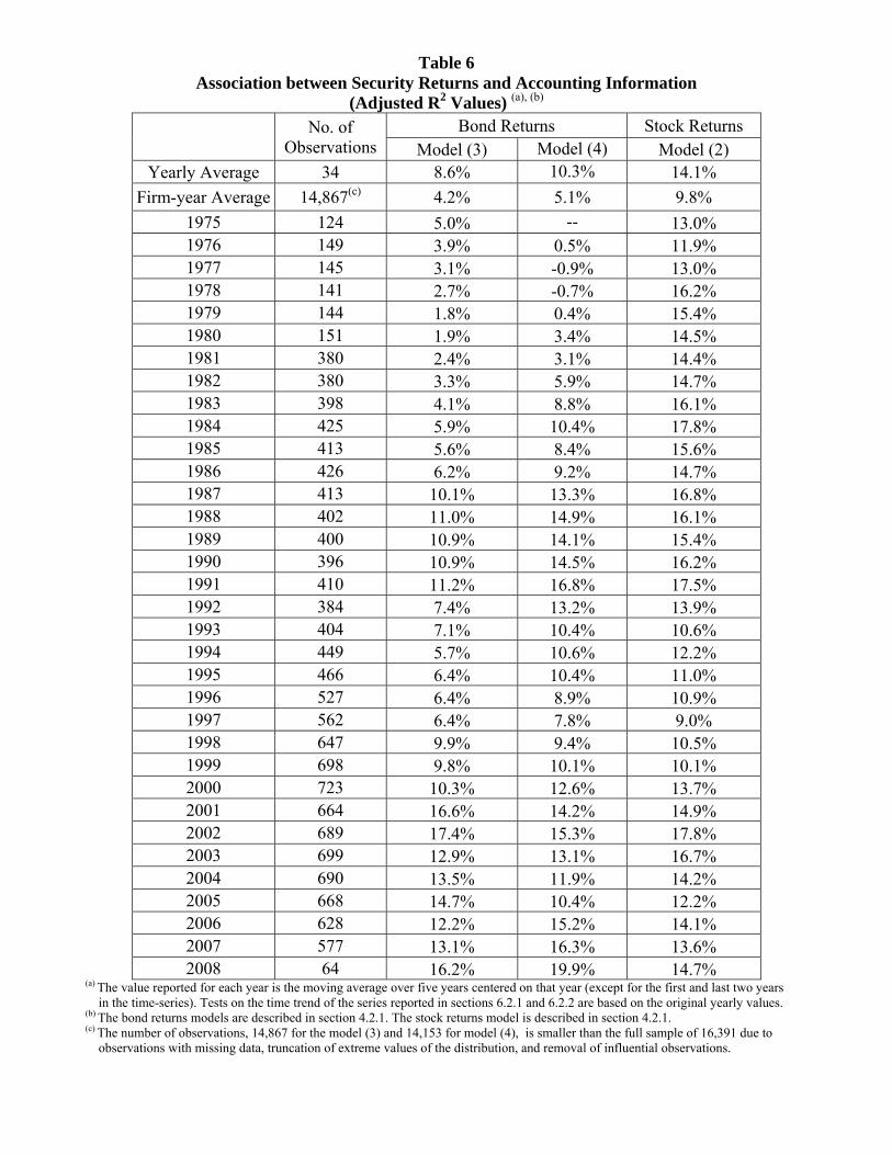
Table 6 Association between Security Returns and Accounting Information
(Adjusted R2 Values) (a), (b)
No. of
Observations Bond Returns Stock Returns
Model (3) Model (4) Model (2) Yearly Average 34 8.6% 10.3% 14.1%
Firm-year Average 14,867(c) 4.2% 5.1% 9.8%
1975 124 5.0% -- 13.0% 1976 149 3.9% 0.5% 11.9% 1977 145 3.1% -0.9% 13.0% 1978 141 2.7% -0.7% 16.2% 1979 144 1.8% 0.4% 15.4% 1980 151 1.9% 3.4% 14.5% 1981 380 2.4% 3.1% 14.4% 1982 380 3.3% 5.9% 14.7% 1983 398 4.1% 8.8% 16.1% 1984 425 5.9% 10.4% 17.8% 1985 413 5.6% 8.4% 15.6% 1986 426 6.2% 9.2% 14.7% 1987 413 10.1% 13.3% 16.8% 1988 402 11.0% 14.9% 16.1% 1989 400 10.9% 14.1% 15.4% 1990 396 10.9% 14.5% 16.2% 1991 410 11.2% 16.8% 17.5% 1992 384 7.4% 13.2% 13.9% 1993 404 7.1% 10.4% 10.6% 1994 449 5.7% 10.6% 12.2% 1995 466 6.4% 10.4% 11.0% 1996 527 6.4% 8.9% 10.9% 1997 562 6.4% 7.8% 9.0% 1998 647 9.9% 9.4% 10.5% 1999 698 9.8% 10.1% 10.1% 2000 723 10.3% 12.6% 13.7% 2001 664 16.6% 14.2% 14.9% 2002 689 17.4% 15.3% 17.8% 2003 699 12.9% 13.1% 16.7% 2004 690 13.5% 11.9% 14.2% 2005 668 14.7% 10.4% 12.2% 2006 628 12.2% 15.2% 14.1% 2007 577 13.1% 16.3% 13.6% 2008 64 16.2% 19.9% 14.7%
(a) The value reported for each year is the moving average over five years centered on that year (except for the first and last two years in the time-series). Tests on the time trend of the series reported in sections 6.2.1 and 6.2.2 are based on the original yearly values.
(b) The bond returns models are described in section 4.2.1. The stock returns model is described in section 4.2.1. (c) The number of observations, 14,867 for the model (3) and 14,153 for model (4), is smaller than the full sample of 16,391 due to
observations with missing data, truncation of extreme values of the distribution, and removal of influential observations.
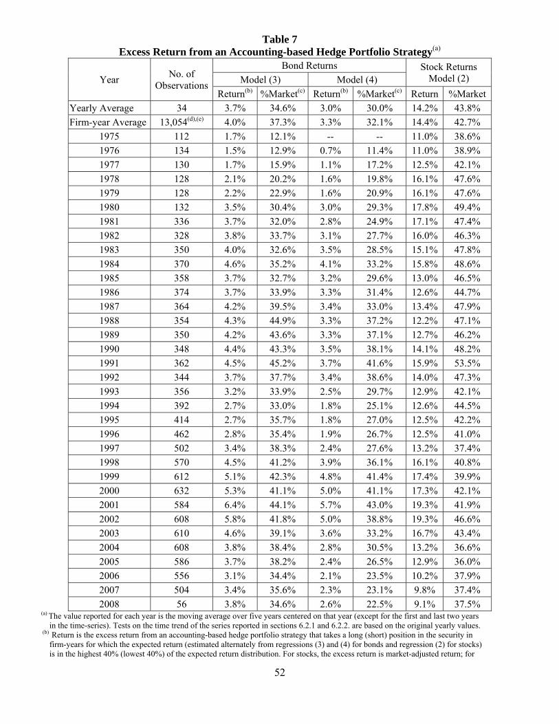
52
Table 7 Excess Return from an Accounting-based Hedge Portfolio Strategy(a)
Year No. of
Observations
Bond Returns Stock Returns Model (2) Model (3) Model (4)
Return(b) %Market(c) Return(b) %Market(c) Return %Market
Yearly Average 34 3.7% 34.6% 3.0% 30.0% 14.2% 43.8%
Firm-year Average 13,054(d),(e) 4.0% 37.3% 3.3% 32.1% 14.4% 42.7%
1975 112 1.7% 12.1% -- -- 11.0% 38.6%
1976 134 1.5% 12.9% 0.7% 11.4% 11.0% 38.9%
1977 130 1.7% 15.9% 1.1% 17.2% 12.5% 42.1%
1978 128 2.1% 20.2% 1.6% 19.8% 16.1% 47.6%
1979 128 2.2% 22.9% 1.6% 20.9% 16.1% 47.6%
1980 132 3.5% 30.4% 3.0% 29.3% 17.8% 49.4%
1981 336 3.7% 32.0% 2.8% 24.9% 17.1% 47.4%
1982 328 3.8% 33.7% 3.1% 27.7% 16.0% 46.3%
1983 350 4.0% 32.6% 3.5% 28.5% 15.1% 47.8%
1984 370 4.6% 35.2% 4.1% 33.2% 15.8% 48.6%
1985 358 3.7% 32.7% 3.2% 29.6% 13.0% 46.5%
1986 374 3.7% 33.9% 3.3% 31.4% 12.6% 44.7%
1987 364 4.2% 39.5% 3.4% 33.0% 13.4% 47.9%
1988 354 4.3% 44.9% 3.3% 37.2% 12.2% 47.1%
1989 350 4.2% 43.6% 3.3% 37.1% 12.7% 46.2%
1990 348 4.4% 43.3% 3.5% 38.1% 14.1% 48.2%
1991 362 4.5% 45.2% 3.7% 41.6% 15.9% 53.5%
1992 344 3.7% 37.7% 3.4% 38.6% 14.0% 47.3%
1993 356 3.2% 33.9% 2.5% 29.7% 12.9% 42.1%
1994 392 2.7% 33.0% 1.8% 25.1% 12.6% 44.5%
1995 414 2.7% 35.7% 1.8% 27.0% 12.5% 42.2%
1996 462 2.8% 35.4% 1.9% 26.7% 12.5% 41.0%
1997 502 3.4% 38.3% 2.4% 27.6% 13.2% 37.4%
1998 570 4.5% 41.2% 3.9% 36.1% 16.1% 40.8%
1999 612 5.1% 42.3% 4.8% 41.4% 17.4% 39.9%
2000 632 5.3% 41.1% 5.0% 41.1% 17.3% 42.1%
2001 584 6.4% 44.1% 5.7% 43.0% 19.3% 41.9%
2002 608 5.8% 41.8% 5.0% 38.8% 19.3% 46.6%
2003 610 4.6% 39.1% 3.6% 33.2% 16.7% 43.4%
2004 608 3.8% 38.4% 2.8% 30.5% 13.2% 36.6%
2005 586 3.7% 38.2% 2.4% 26.5% 12.9% 36.0%
2006 556 3.1% 34.4% 2.1% 23.5% 10.2% 37.9%
2007 504 3.4% 35.6% 2.3% 23.1% 9.8% 37.4%
2008 56 3.8% 34.6% 2.6% 22.5% 9.1% 37.5% (a) The value reported for each year is the moving average over five years centered on that year (except for the first and last two years
in the time-series). Tests on the time trend of the series reported in sections 6.2.1 and 6.2.2. are based on the original yearly values. (b) Return is the excess return from an accounting-based hedge portfolio strategy that takes a long (short) position in the security in
firm-years for which the expected return (estimated alternately from regressions (3) and (4) for bonds and regression (2) for stocks) is in the highest 40% (lowest 40%) of the expected return distribution. For stocks, the excess return is market-adjusted return; for

53
bonds, the excess return is the difference between the bond’s return and the return on Treasury notes matched on the bond’s time-to-maturity and coupon rate (see section 4.2.3).
(c) %Market is the fraction that the excess return from the accounting-based strategy constitutes of the contemporaneous excess return that could be obtained through perfect foresight of the sign of the security’s excess return ((see section 4.2.3).
(d) The number of observations is smaller than 16,391, the full sample, due to missing data (107 observations), and due to the computation of the %Market that does not consider 20% of the observations – see section 4.2.3 (representing 3,230 observations).
(e) The number of observations for the Bond Return model (4) is 11,352, which is smaller than 16,391, the full sample, due to missing data (2,201 observations), and due to the computation of the %Market that does not consider 20% of the observations (representing 2,838 observations) – see section 4.2.3.for the computation of %Market.
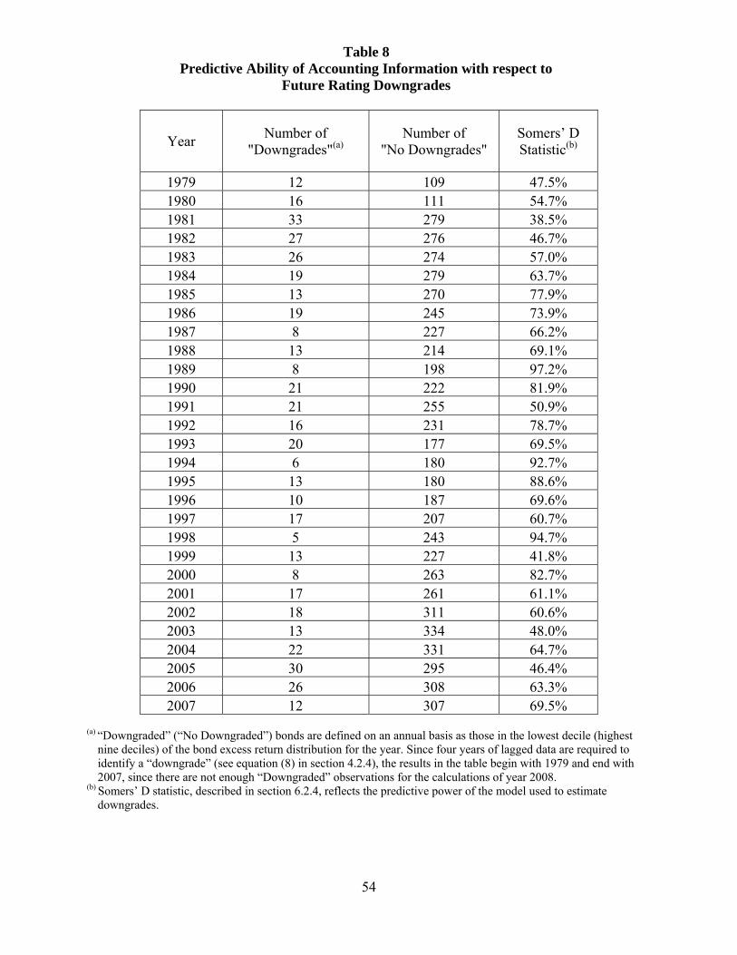
54
Table 8 Predictive Ability of Accounting Information with respect to
Future Rating Downgrades
Year Number of
"Downgrades"(a) Number of
"No Downgrades" Somers’ D Statistic(b)
1979 12 109 47.5% 1980 16 111 54.7% 1981 33 279 38.5% 1982 27 276 46.7% 1983 26 274 57.0% 1984 19 279 63.7% 1985 13 270 77.9% 1986 19 245 73.9% 1987 8 227 66.2% 1988 13 214 69.1% 1989 8 198 97.2% 1990 21 222 81.9% 1991 21 255 50.9% 1992 16 231 78.7% 1993 20 177 69.5% 1994 6 180 92.7% 1995 13 180 88.6% 1996 10 187 69.6% 1997 17 207 60.7% 1998 5 243 94.7% 1999 13 227 41.8% 2000 8 263 82.7% 2001 17 261 61.1% 2002 18 311 60.6% 2003 13 334 48.0% 2004 22 331 64.7% 2005 30 295 46.4% 2006 26 308 63.3% 2007 12 307 69.5%
(a) “Downgraded” (“No Downgraded”) bonds are defined on an annual basis as those in the lowest decile (highest
nine deciles) of the bond excess return distribution for the year. Since four years of lagged data are required to identify a “downgrade” (see equation (8) in section 4.2.4), the results in the table begin with 1979 and end with 2007, since there are not enough “Downgraded” observations for the calculations of year 2008.
(b) Somers’ D statistic, described in section 6.2.4, reflects the predictive power of the model used to estimate downgrades.
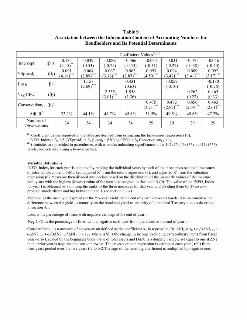
Table 9 Association between the Information Content of Accounting Numbers for
Bondholders and Its Potential Determinants
Coefficient Values(a),(b)
Intercept, (β0) 0.184
(2.15)** 0.049 (0.53)
-0.089 (-0.75)
-0.066 (-0.53)
-0.034 (-0.31)
-0.031 (-0.27)
-0.051 (-0.38)
-0.056 (-0.40)
YSpreadt (β1)
0.091 (4.18)***
0.064 (2.89)***
0.067 (3.16)***
0.063 (2.87)***
0.093 (4.50)***
0.094 (3.42)***
0.089 (3.41)***
0.092 (3.17)***
Losst (β2) 1.157
(2.69)*** 0.431 (0.63)
-0.059 (-0.10)
-0.180 (-0.26)
Neg CFOt (β3)
2.535 (3.01)***
1.858 (1.36)
0.262 (0.22)
0.465 (0.33)
Conservatismt-1 (β4)
0.475 (3.21)***
0.482 (2.93)***
0.456 (2.64)**
0.463 (2.61)**
Adj. R2 33.3% 44.1% 46.7% 45.6% 51.5% 49.5% 49.6% 47.7%
Number of Observations
34 34 34 34 29 29 29 29
(a) Coefficient values reported in the table are derived from estimating the time-series regression (10): INFO_Indext = β0 + β1(YSpread)t + β2 (Loss)t + β3(Neg CFO)t + β4 Conservatismt-1 + υt. (b) t-statistics are provided in parentheses, with asterisks indicating significance at the 10% (*), 5% (**) and 1% (***) levels, respectively, using a two-tailed test.
Variable Definitions INFO_Indext for each year is obtained by ranking the individual years by each of the three cross-sectional measures of information content, %Market, adjusted R2 from the return regression (3), and adjusted R2 from the valuation regression (6). Years are then divided into deciles based on the distribution of the 34 yearly values of the measure, with years with the highest (lowest) value of the measure assigned to the decile 9 (0). The value of the INFO_Index for year t is obtained by summing the ranks of the three measures for that year and dividing them by 27 so as to produce standardized ranking between 0 and 1(see section 6.2.4).
YSpreadt is the mean yield spread (or the “excess” yield) at the end of year t across all bonds. It is measured as the difference between the yield-to-maturity on the bond and yield-to-maturity of a matched Treasury note as described in section 4.1.
Losst is the percentage of firms with negative earnings at the end of year t. Neg CFOt is the percentage of firms with a negative cash flow from operations at the end of year t.
Conservatismt-1 is a measure of conservatism defined as the coefficient 3 in regression (9): NIi,t = 0 + 1DNIi, t-1 +
2NI i, t-1 + 3DNI i, t-1*NI i, t-1 + i, t where NI is the change in income excluding extraordinary items from fiscal year t-1 to t, scaled by the beginning book value of total assets and DNI is a dummy variable set equal to one if NI in the prior year is negative and zero otherwise. The cross-sectional regression is estimated each year ( t=0) from firm-years pooled over the five years t-2 to t+2.The sign of the resulting coefficient is multiplied by negative one.
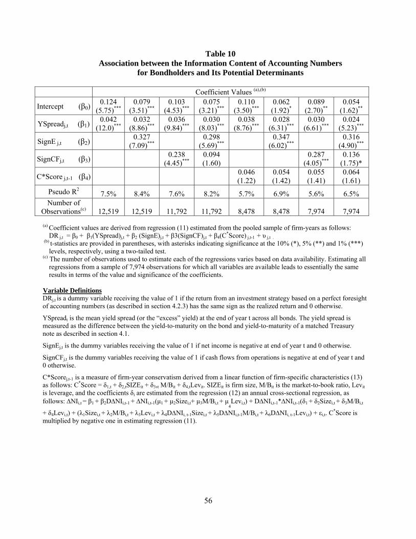
56
Table 10 Association between the Information Content of Accounting Numbers
for Bondholders and Its Potential Determinants
Coefficient Values (a),(b)
Intercept (β0) 0.124
(5.75)*** 0.079
(3.51)*** 0.103
(4.53)*** 0.075
(3.21)*** 0.110
(3.50)***0.062(1.92)*
0.089 (2.70)**
0.054(1.62)**
YSpreadj,t (β1)
0.042 (12.0)***
0.032 (8.86)***
0.036 (9.84)***
0.030 (8.03)***
0.038(8.76)***
0.028(6.31)***
0.030 (6.61)***
0.024(5.23)***
SignE j,t (β2) 0.327
(7.09)*** 0.298
(5.69)*** 0.347
(6.02)*** 0.316
(4.90)***
SignCFj,t (β3)
0.238 (4.45)***
0.094 (1.60)
0.287 (4.05)***
0.136(1.75)*
C*Score j,t-1 (β4)
0.046(1.22)
0.054(1.42)
0.055 (1.41)
0.064(1.61)
Pseudo R2 7.5% 8.4% 7.6% 8.2% 5.7% 6.9% 5.6% 6.5%Number of
Observations(c) 12,519 12,519 11,792 11,792 8,478 8,478 7,974 7,974
(a) Coefficient values are derived from regression (11) estimated from the pooled sample of firm-years as follows: DR j,t = β0 + β1(YSpread)j,t + β2 (SignE)j,t + β3(SignCF)j,t + β4(C
*Score) j,t-1 + υ j,t . (b) t-statistics are provided in parentheses, with asterisks indicating significance at the 10% (*), 5% (**) and 1% (***)
levels, respectively, using a two-tailed test. (c) The number of observations used to estimate each of the regressions varies based on data availability. Estimating all
regressions from a sample of 7,974 observations for which all variables are available leads to essentially the same results in terms of the value and significance of the coefficients.
Variable Definitions DRj,t is a dummy variable receiving the value of 1 if the return from an investment strategy based on a perfect foresight of accounting numbers (as described in section 4.2.3) has the same sign as the realized return and 0 otherwise.
YSpreadt is the mean yield spread (or the “excess” yield) at the end of year t across all bonds. The yield spread is measured as the difference between the yield-to-maturity on the bond and yield-to-maturity of a matched Treasury note as described in section 4.1.
SignEj,t is the dummy variables receiving the value of 1 if net income is negative at end of year t and 0 otherwise.
SignCFj,t is the dummy variables receiving the value of 1 if cash flows from operations is negative at end of year t and 0 otherwise.
C*Scorej,t-1 is a measure of firm-year conservatism derived from a linear function of firm-specific characteristics (13) as follows: C*Score = δ1,t + δ2,tSIZEit + δ3,t M/Bit + δ4,tLevit. SIZEit is firm size, M/Bit is the market-to-book ratio, Levit is leverage, and the coefficients δi are estimated from the regression (12) an annual cross-sectional regression, as follows: NIi,t
= β1
+ β2DNIi,t-1
+ NIi,t-1(μ1
+ μ2Sizei,t+ μ3M/Bi,t
+ μ
4Levi,t) + DNIi,t-1*NIi,t-1(δ1
+ δ2Sizei,t
+ δ3M/Bi,t
+ δ4Levi,t) + (λ1Sizei,t + λ2M/Bi,t
+ λ3Levi,t
+ λ4DNIi, t-1Sizei,t
+ λ5DNIi,t-1M/Bi,t
+ λ6DNIi, t-1Levi,t) + εi,t. C
*Score is multiplied by negative one in estimating regression (11).