THE CHARACTERISTICS MATRIX AS A TOOL FOR ANALYSING …

HAL Id: hal-00512896https://hal.archives-ouvertes.fr/hal-00512896

Submitted on 1 Sep 2010

HAL is a multi-disciplinary open accessarchive for the deposit and dissemination of sci-entific research documents, whether they are pub-lished or not. The documents may come fromteaching and research institutions in France orabroad, or from public or private research centers.

L’archive ouverte pluridisciplinaire HAL, estdestinée au dépôt et à la diffusion de documentsscientifiques de niveau recherche, publiés ou non,émanant des établissements d’enseignement et derecherche français ou étrangers, des laboratoirespublics ou privés.

THE CHARACTERISTICS MATRIX AS A TOOLFOR ANALYSING PROCESS STRUCTURE

Andres Carrion Garcia, J M Jabaloyes, Aura Lopez

To cite this version:Andres Carrion Garcia, J M Jabaloyes, Aura Lopez. THE CHARACTERISTICS MATRIX AS ATOOL FOR ANALYSING PROCESS STRUCTURE. International Journal of Production Research,Taylor & Francis, 2007, 45 (02), pp.385-400. �10.1080/00207540600644880�. �hal-00512896�

https://hal.archives-ouvertes.fr/hal-00512896

https://hal.archives-ouvertes.fr

For Peer Review O

nly

THE CHARACTERISTICS MATRIX AS A TOOL FOR ANALYSING

PROCESS STRUCTURE

Journal: International Journal of Production Research

Manuscript ID: TPRS-2005-IJPR-0463

Manuscript Type: Original Manuscript

Date Submitted by the Author:

22-Nov-2005

Complete List of Authors: CARRION GARCIA, ANDRES; Universidad Politecnica, Applied Statistics, O.R. and Quality Jabaloyes, J M; Polytechnic University of Valencia, Department of Statistics Lopez, Aura; Universidad Javeriana, Industrial Engineering

Keywords: PROCESSES, PROCESS CONTROL

Keywords (user): Mic-Mac Method, Characteristics Matrix

http://mc.manuscriptcentral.com/tprs Email: [email protected]

International Journal of Production Research

For Peer Review O

nly

THE CHARACTERISTICS MATRIX AS A TOOL FOR ANALYSING PROCESS STRUCTURE

Andrés CarriónA1†*, José Jabaloyes A1* and Aura López A2*

A1Polytechnic University of Valencia. Camino de Vera s/n, 46022 Valencia, Spain. A2Pontificia Universidad Javeriana, Calle 18 No. 118-250 Av. Cañasgordas, Cali (Colombia).

ABSTRACT

The characteristics matrix is a tool to describe the relationship between product characteristics and process operations. It has been used traditionally with only descriptive purposes and analysed with a very limited intuitive approach. In this paper we present a methodology to analyse deeply the process structure using the information contained in the characteristics matrix. We apply the principles of the mic-mac method to study both direct and indirect internal relations, defining importance criteria and identifying the most important characteristics and operations. Keywords: Quality; Processes; Mic-Mac Method; Process control; Characteristics Matrix 1. The role of the characteristics matrix in quality control. Quality control in production processes requires the observation of some product characteristics, usually by means of control charts. With these charts we are able to monitor the evolution of the quality characteristic and detect the anomalous conditions that may arise. However, there is an important stage, previous to the use of control charts, a less studied stage despite its great importance: the selection of the characteristics to control. Obviously, it is impossible to control all the product characteristics (dimensional, mechanical, electrical, …) therefore, it is necessary to select only a few of them. But the question is, which ones? The correct answer is obvious: the most important characteristics should be controlled. The question now is how to select these ‘important’ characteristics and how to measure their importance. To do this, we have to take into account different aspects of the characteristics’ importance: importance for the product function, for the production process and for the customer. If we consider the first two elements, it is evident that we need a deep knowledge of the product and process at the moment of selecting the characteristics to control. The characteristics matrix is a useful tool for this purpose. This matrix provides a fine and simple description of the production process and the effect that successive operations have on the product. The characteristics matrix (CM), usually a non square matrix, displays in rows † Correspondence: acarrió[email protected] Postal address: Andrés Carrión. Departamento de Estadística e Investigación Operativa Aplicadas y Calidad. Universidad Politécnica de Valencia. Camino de Vera s/n 46022 – Valencia- Spain. • Dr Carrión is Director of the Department of Applied Statistics, O.R. and Quality of the Polytechnic

University of Valencia (Spain). He is member of the Spanish Society for Quality (AEC). acarrió[email protected]

• Dr Jabaloyes is Professor in the Department of Applied Statistics, O.R. and Quality of the Polytechnic University of Valencia (Spain). [email protected]

• Dr López is Professor of the Faculty of Engineering of the Pontificia Universidad Javeriana of Cali (Colombia). [email protected]

Page 1 of 45



123456789101112131415161718192021222324252627282930313233343536373839404142434445464748495051525354555657585960

For Peer Review O

nly

2

the different process operations and in columns the product characteristics that are produced or used in the process operations. For example, in mechanization processes, most of the product characteristics are dimensional parameters. This matrix is used by different industrial procedures like Dimensional Control Plans (DCP), FMC (1985), and Advanced Product Quality Planning (APQP), AIAG (1995). Carrión and Jabaloyes (1995) presented a first study of the possibilities of this matrix for further analysis. The general term of the CM, aij , is the kind of relations between the corresponding process operation (row i) and product characteristic (column j). Usually a set of symbols is used to represent this relation. The three most frequently used and most important are: x characteristic created or modified in this operation. L characteristic used for locating the part. C characteristic used for clamping the part. The use of that matrix is limited to its observation and to the intuitive evaluation of its contents, as it is like a map of the production process, and to the identification of the characteristics and more influential operations by simple inspection of the matrix. Table 1 in the example shows a simple example of such matrix. The objective of this paper is to exploit the information contained in the characteristics matrix via a procedure based on the technological forecast mic-mac method (Duperrin and Godet, 1974; Godet 1991). In this method we consider a square matrix that places the variables affecting a certain system in rows and columns, and the matrix general term measures, in a subjective scale, the degree of influence among characteristics. Successive powers of that matrix permit to detect indirect relations among variables, that were not evident in the original matrix. 2. Study and analysis of the C.M. Let’s consider a production process which includes m operations, and a product described by n quality characteristics. The characteristics matrix, as previously defined, will have m·n dimensions. For the study and analysis of the characteristics matrix, it is useful to separate the information of the matrix in two matrices with equal dimensions: the first one is called “changes matrix” and it contains the information related to the characteristics created or modified in each operation (corresponding to the code x of the traditional CM). The second one is called “LC matrix”, and it contains the information related to operations of locating and clamping (identified with the codes L and C in the traditional CM). In both matrices, the codes are substituted by 1 (one), remaining the rest of the terms in zero. We will then have two matrices, usually of very low density, that collect the information on the process and the characteristics of the product. Operating with these matrices, we will obtain more information on the structure of the process and the relations between characteristics. 3. The matrix of changes. First, let’s consider this matrix that collects the information of changes in product characteristics. If we call this changes matrix X, its general term xij is:

xij = 1 if characteristic j has been created or modified in the operation i

Page 2 of 45



123456789101112131415161718192021222324252627282930313233343536373839404142434445464748495051525354555657585960

For Peer Review O

nly

3

xij = 0 in other cases If we post-multiply it by its transposed X’, the result is a symmetric square matrix with m·m size (where m is the number of process operations):

X X’ = C The general term for this matrix C, cij, is:

cij = ∑=

n

1kjkik xx

the values of cij represents:

• if i=j, cij is the number of characteristics created or modified in the operation i • if i≠j, cij is the number of common characteristics changed in both operations, i and

j.

We can also see that:

• The sum of the elements in row i, ∑=

n

1jijc , is the number of changes that are produced

in the characteristics changed in that operation i, that is, the changes that are produced in the operation i plus the changes in other operations that affect the characteristics modified in operation i.

• The matrix trace C is the number of change actions that have been carried out in the process.

If we multiply now in the opposite order:

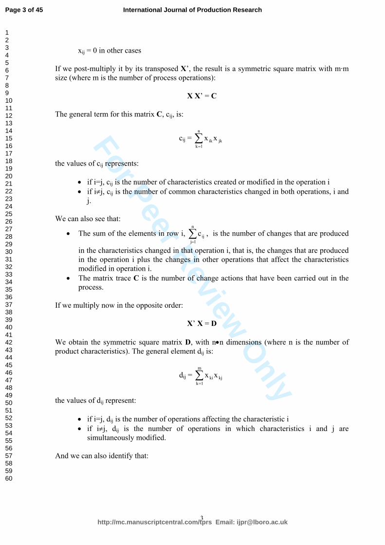
X’ X = D We obtain the symmetric square matrix D, with n•n dimensions (where n is the number of product characteristics). The general element dij is:

dij = ∑=

m

1kkjki xx

the values of dij represent:

• if i=j, dij is the number of operations affecting the characteristic i • if i≠j, dij is the number of operations in which characteristics i and j are

simultaneously modified. And we can also identify that:

Page 3 of 45



123456789101112131415161718192021222324252627282930313233343536373839404142434445464748495051525354555657585960

For Peer Review O

nly

4

• The sum of row i, ∑=

m

1jijd , is the number of changes related to characteristic i,

produced in this characteristic or in any other characteristic and operation (that is: changes in characteristic i, plus changes in other characteristics that have changes simultaneously with i).

• As in C, the D matrix trace is the number of change actions performed in the process.

4. The LC Matrix. If we call the LC Matrix B, we can work in the same way as with the Change Matrix X. If the general term of B, bij is:

bij = 1 if the characteristic j has been used for location or clamping (LC) in the operation i bij = 0 in other cases

If we post-multiply B by its transposed, we obtain a new symmetric square matrix E with m·m dimensions, where m is the number of operations in the process:

B B’ = E The general term eij is:

eij = ∑=

n

1kjkik bb

the values of eij represent:

• if i=j, eij is the number of characteristics used for LC in operation i • if i≠j, eij is the number of common characteristics shared by operations i and j for

LC

Also, we can see that:


n

1jije , is the number of characteristics used for LC

actions that are related to operation i. That is, the LC actions carried out in the operation i plus the LC actions in other operations that use characteristics also used in operation i.

• The matrix trace E is the number of LC actions that have been carried out in the process.

If we pre-multiply B by its transposed:

B’ B = F We obtain the matrix F, a symmetrical square matrix, with dimensions n•n (where n is the number of characteristics). The general term of F is:

Page 4 of 45



123456789101112131415161718192021222324252627282930313233343536373839404142434445464748495051525354555657585960

For Peer Review O

nly

5

fij = ∑=

m

1kkjkibb

the values of fij represent:

• if i=j, fij is the number of operations that use characteristic i for LC • if i≠j, fij is the number of operations in which characteristics i and j are

simultaneously used for LC. And we can also identify that:


m

1jijf , is the number of LC actions related with the

characteristic i, referred to this characteristic or to any other characteristic acting together with characteristic i.

• The matrix trace F is the number of LC actions performed in the process. 5. Combination of the L/C and Changes Matrices. The information previously obtained is interesting as it describes some non evident aspects of the production process structure, but is the joint use of both matrices what gives us the best results. In the following paragraphs we will present some of these results. 5.1. Influences between operations and between characteristics. 5.1.1 First-order influences. A) First-order relationship between operations

If we post-multiply the L/C matrix by the transposed of the changes matrix:

B X’ = G We obtain a non symmetric square matrix G, with as many rows and columns as operations in the process. The general term, gij ,is:

bij = ∑=

m

1kjkik xb

And we can find that:

• If i ≠ j, gij is the number of characteristics used for L/C in the operation i that were changed in the operation j. It establishes whether there is influence of operation j on operation i, and, to a certain extent, the potential intensity of that influence (by the reiteration).

• If i = j, usually gij will be null, as it represents the number of times that a characteristic is employed for L/C is changed in that same operation.

Page 5 of 45



123456789101112131415161718192021222324252627282930313233343536373839404142434445464748495051525354555657585960

For Peer Review O

nly

6

The number of non zero elements of column j is the number of operations influenced by the operation j through L/C. B) First-order relationship between characteristics If we now pre-multiply the L/C matrix by the transposed of the changes matrix, we obtain a new non symmetric square matrix, H, with as many rows or columns as characteristics of the part under study.

X’ B = H The general term hij is:

hij = ∑=

m

1kjkik bx

where:

• If i ≠ j, hij is the number of times that characteristic I is modified using characteristic j for L/C. It establishes whether there is influence of characteristic j on characteristic i, and, to a certain extent, the potential intensity of that influence (by the reiteration).

• If i = j, usually hij will be null The number of non zero elements in column j represents the number of characteristics influenced by the characteristic j, via L/C. 5.1.2. Second-order influences. A) Second-order relationship between operations In the two previous cases, the influences identified are of first-order, in the sense that are direct influences of an operation (or characteristic) on another. We can be interested in the indirect influences. If we take now the square matrix G and we multiply it by itself, we obtain a new matrix that collects the second-order influences of operation j on operation i, that is, influences between two operations with a third intermediate operations (e.g.: op1 influencing op2, and op2 influencing op3, and as a consequence, indirect influence of op1 on op3):

G G = K Where the general term kij is the number of single intermediate influences of operation j on operation i. B) Second-order relationship between characteristics In a similar way, we can obtain:

Page 6 of 45



123456789101112131415161718192021222324252627282930313233343536373839404142434445464748495051525354555657585960

For Peer Review O

nly

7

H H = L

Where L is a square matrix with as many dimensions as characteristics, and whose general term lij is the number of second-order influences, that is, influences between two characteristics (characteristics j on characteristic i) with a third one as intermediate. 5.1.3. Upper-order influences. We can obtain influences of third, fourth or upper-order simply by multiplying the appropriate number of times each of the matrices G and H; for the third-order influences between operations we have to calculate G G G, and for influences between characteristics H H H; for the fourth-order influences between operations we have to calculate G G G G, and for influences between characteristics H H H H; and so on. At a certain point, depending on the complexity of process and product, those matrices will be null, indicating that there are no relations of that order, neither upper-order, among operations or characteristics. The highest order corresponds to the number of operations for one case and to the number of characteristics for the other. 5.1.3. Global influences evaluation. If we sum these matrices obtained as successive power of G until obtaining the null matrix, we obtain:

P = G + G G + G G G + ... Where P is a square matrix (dimensions m•m), that includes the relationships of any order between process operations:

• pij, if i ≠ j, is the number of direct or indirect influences of operation j on operation i.

• pij, if i = j, is zero. • ∑

jijp = number of influences, direct or indirect, affecting operation i.

• ∑i

ijp = number of influences, direct or indirect, generated by operation j.

In the same way, we can evaluate relations among characteristics obtaining:

Q = H + H H + H H H + ... where Q is a square matrix (dimensions n•n) whose general element is:

• qij, if i ≠ j, is the number of direct or indirect influence ways of characteristic j on characteristic i.

• qij, si i = j, is zero. • ∑

jijq = number of influences, direct or indirect, affecting characteristic i.

Page 7 of 45



123456789101112131415161718192021222324252627282930313233343536373839404142434445464748495051525354555657585960

For Peer Review O

nly

8

• ∑i

ijq = number of influences, direct or indirect, generated by characteristic j.

6. Influence chart. In the mic-mac method the concepts of motricity and dependence are defined and used. The first one refers to the degree of influence that one variable has over the others. The dependence is the degree to which one variable is influenced by the others. The same idea can be used here, referred both to process operations and to product characteristics. The motricity will be the sum by columns and the dependence the sum by rows of the corresponding matrices P and Q. If we consider the matrix P, relations between operations, we have that

pijj∑

is the number of influences received by the operation i from all the other operations, that is, its dependence. Also in matrix P, we have that

piji∑

is the number of influences generated by the operation j, that is its motricity. The same operations can be done in matrix Q, obtaining in this way the dependence and motricity for each characteristic. With these pairs of data, we can prepare an XY plot, having in x-axis the motricity and in y-axis the dependence. This graphic is a plot of the nature of the inter-operations (or inter-characteristics) relationships in the process. Operations with high motricity and low dependence are the operation with higher influence over the others and, at the same time, less influenced by others. Usually this kind of operations will be at the beginning of the process. Its control is very important due to its great influence over subsequent operations and, in general, over the process. We can understand these as “source operations”. In the opposite corner, we have operations with low motricity and high dependence. These can be called “result operations”, very influenced by the rest of the process and usually difficult to control. For the influences between characteristics we can also outline the corresponding motricity/dependence plot. As in the previous chart, characteristics with high motricity and low dependence are those with important influence over the others, but, on the other hand, not influenced by the rest of the process. These can be called “source characteristics”. Quality problems in one of these characteristics tend to move along the process affecting other characteristics. In the opposite situations we have characteristics with low motricity and high dependence, highly influenced by other product characteristics and usually difficult to control. We can name these as “result characteristics”.

Page 8 of 45



123456789101112131415161718192021222324252627282930313233343536373839404142434445464748495051525354555657585960

For Peer Review O

nly

9

7. Conclusions. The analysis of the characteristics matrix has proven to provide important information about the process, the internal relationship structure between operations and between characteristics. In this way, this matrix is an interesting procedure to study and understand this complex relationship structure. With its help, and with simple operations we can distinguish the most influential operations and characteristics, and use this information to carefully control these activities, as any problem that appears here will spread over the process, affecting other operations and characteristics. We can also identify other operations or characteristics that will be, in advance, difficult to control, as they are the effect of many sources of variation. Control on these operations or characteristics needs to take into account that in many cases problem solving need to focus on operations or characteristics different to the places where the problem has been detected. 8. Example The case defined in Table 1 is a simple example of the application of the procedure described before to a mechanising process.

C.1 C.2 C.3 C.4 C.5 C.6 C.7 C.8 C.9 C.10 C.11 C.12 C.13 OP.1 X X OP.2 L C X X OP.3 C L X X X OP.4 C L X X X X OP.5 L C X X X X

Table 1. Characteristic Matrix of a simple process. This process can be described, basing on Table 1, as follows:

1. In Operation 1 we receive raw parts with characteristics C.1 and C.2 2. In Op. 2 characteristic C.1 is used for locating, C.2 is used for clamping and

characteristics C.3 and C.6 are created. 3. In Op. 3 characteristic C.2 is used again for clamping, C.3 for locating and

characteristics C.4, C.5 and C.7 are created or modified. 4. In Op. 4 again C.2 is used for clamping and C.3 for locating, and C.5, C.8, C.9 and

C.13 are created or modified. 5. Finally, in Op. 5 characteristic C.3 is used for locating, C.7 for clamping and

characteristics C.10, C.11, C.12 and C.13 are created or modified. With this table we can build the two matrices that we have called “matrix of changes” and “L/C matrix”. The changes matrix is represented in Table 2. and L/C matrix in Table 3.:

C.1 C.2 C.3 C.4 C.5 C.6 C.7 C.8 C.9 C.10 C.11 C.12 C.13 OP.1 1 1 0 0 0 0 0 0 0 0 0 0 0 OP.2 0 0 1 0 0 1 0 0 0 0 0 0 0

Page 9 of 45



123456789101112131415161718192021222324252627282930313233343536373839404142434445464748495051525354555657585960

For Peer Review O

nly

10

OP.3 0 0 0 1 1 0 1 0 0 0 0 0 0 OP.4 0 0 0 0 1 0 0 1 1 0 0 0 1 OP.5 0 0 0 0 0 0 0 0 0 1 1 1 1

Table 2. Changes Matrix X. Characteristics creation or modification

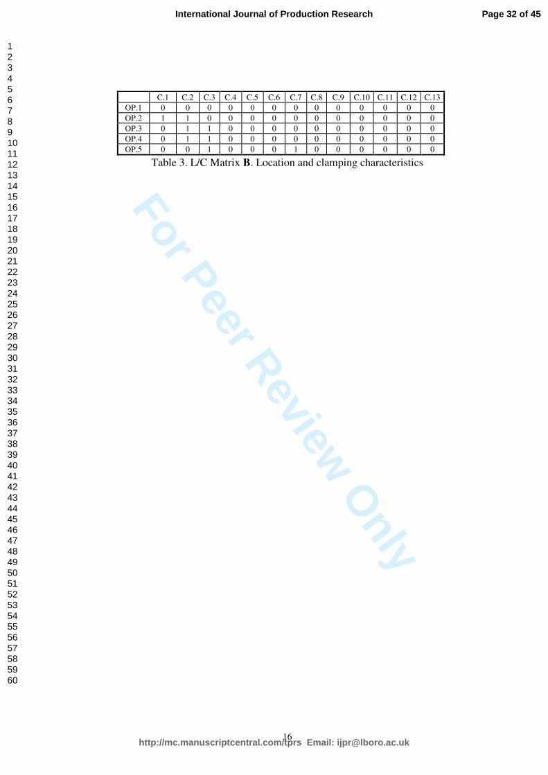
C.1 C.2 C.3 C.4 C.5 C.6 C.7 C.8 C.9 C.10 C.11 C.12 C.13 OP.1 0 0 0 0 0 0 0 0 0 0 0 0 0 OP.2 1 1 0 0 0 0 0 0 0 0 0 0 0 OP.3 0 1 1 0 0 0 0 0 0 0 0 0 0 OP.4 0 1 1 0 0 0 0 0 0 0 0 0 0 OP.5 0 0 1 0 0 0 1 0 0 0 0 0 0

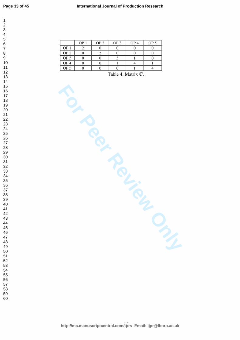
Table 3. L/C Matrix B. Location and clamping characteristics Working with the changes matrix X, and to study the relations between operations we will compute the product XX’, obtaining the square matrix C, shown in Table 4.

OP 1 OP 2 OP 3 OP 4 OP 5 OP 1 2 0 0 0 0 OP 2 0 2 0 0 0 OP 3 0 0 3 1 0 OP 4 0 0 1 4 1 OP 5 0 0 0 1 4

Table 4. Matrix C. We can see here that, for instance:

• in Operation 2 there have been changed (created or modified) two characteristics (element 2,2 of the matrix): in Table 1 we can confirm that this two characteristics are C.3 and C.6.

• in Operation 5 four characteristics have been changed (element 5,5 of the matrix): in Table 1 we can see that these characteristics are C.10, C.11, C.12 and C.13.

• We can read that there is one common characteristic changed in operations 3 and 4 (element 4,3 or 3,4 of the matrix): in Table 1 we verify that this characteristic is C.5, that was created in operation 3 and modified in operation 4.

If we change the order of the product that we have made to obtain matrix C, we will have matrix D = X’X, presented in Table 5.:

Page 10 of 45



123456789101112131415161718192021222324252627282930313233343536373839404142434445464748495051525354555657585960

For Peer Review O

nly

11

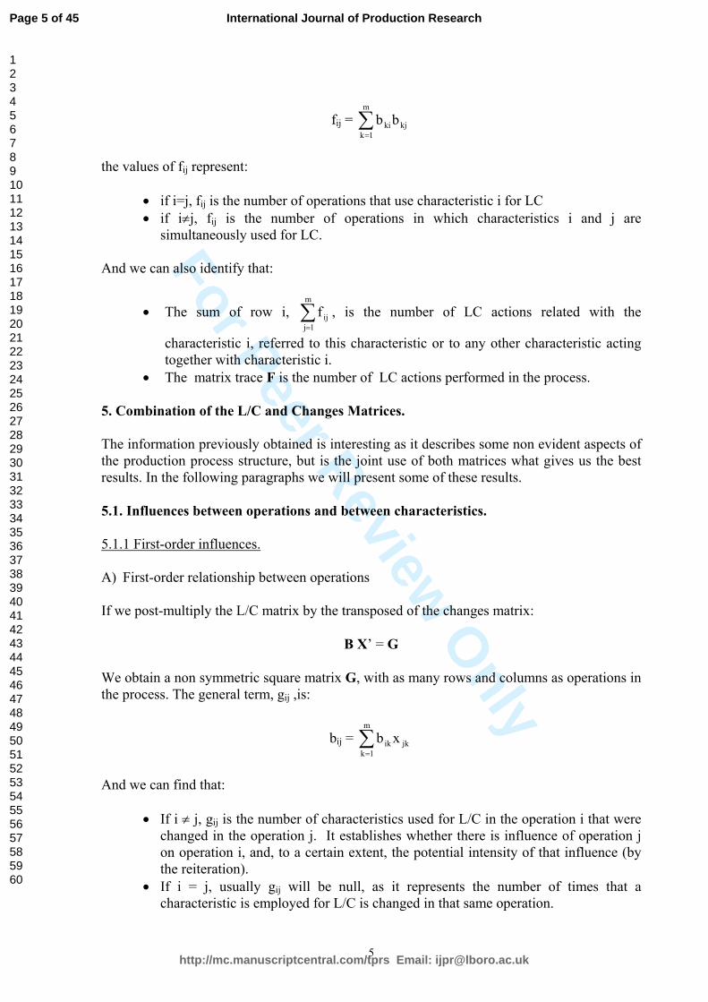
C 1 C 2 C 3 C 4 C 5 C 6 C 7 C 8 C 9 C10 C11 C12 C13 C 1 1 1 C 2 1 1 C 3 1 1 C 4 1 1 1 C 5 1 2 1 1 1 1 C 6 1 1 C 7 1 1 1 C 8 1 1 1 1 C 9 1 1 1 1 C 10 1 1 1 1 C 11 1 1 1 1 C 12 1 1 1 1 C 13 1 1 1 1 1 1 2

Table 5. Matrix D. In Table 5 zeroes have been omitted for easier reading of the table. These criteria will be used from now on. As examples, we can see in Table 5 that:

• Characteristic 3 is affected by only one operation (element 3,3 of the matrix): In Table 1 we read that this operation is Op. 2.

• Characteristic 5 is affected by two operations (element 5,5 of the matrix): In Table 1 we read that these two operations are Op. 3 and Op. 4.

• If we have a look outside the diagonal, we find that characteristics 6 and 3 have changed together in one operation (element 3,6 of the matrix): In table 1 we read that this operations is Op. 2. It also occurs with many others as characteristics 1 and 2 or 11 and 12 (elements 1,2 and 11,12 of the matrix).

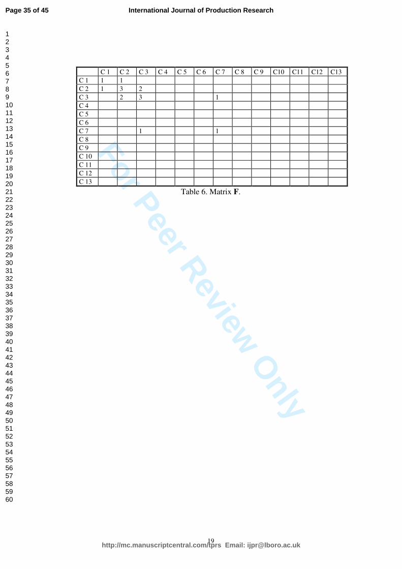
Working now with the L/C matrix, we can obtain matrices F and G from:

B’B = F B B’ = E In Tables 6 and 7 we present these matrices for the case studied as example: C 1 C 2 C 3 C 4 C 5 C 6 C 7 C 8 C 9 C10 C11 C12 C13 C 1 1 1 C 2 1 3 2 C 3 2 3 1 C 4 C 5 C 6 C 7 1 1 C 8 C 9 C 10 C 11 C 12 C 13

Table 6. Matrix F.

Page 11 of 45



123456789101112131415161718192021222324252627282930313233343536373839404142434445464748495051525354555657585960

For Peer Review O

nly

12

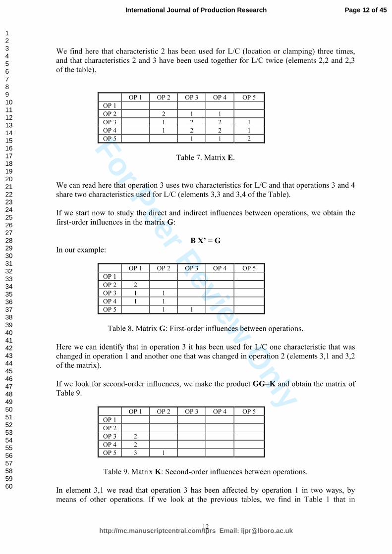
We find here that characteristic 2 has been used for L/C (location or clamping) three times, and that characteristics 2 and 3 have been used together for L/C twice (elements 2,2 and 2,3 of the table).

OP 1 OP 2 OP 3 OP 4 OP 5 OP 1 OP 2 2 1 1 OP 3 1 2 2 1 OP 4 1 2 2 1 OP 5 1 1 2

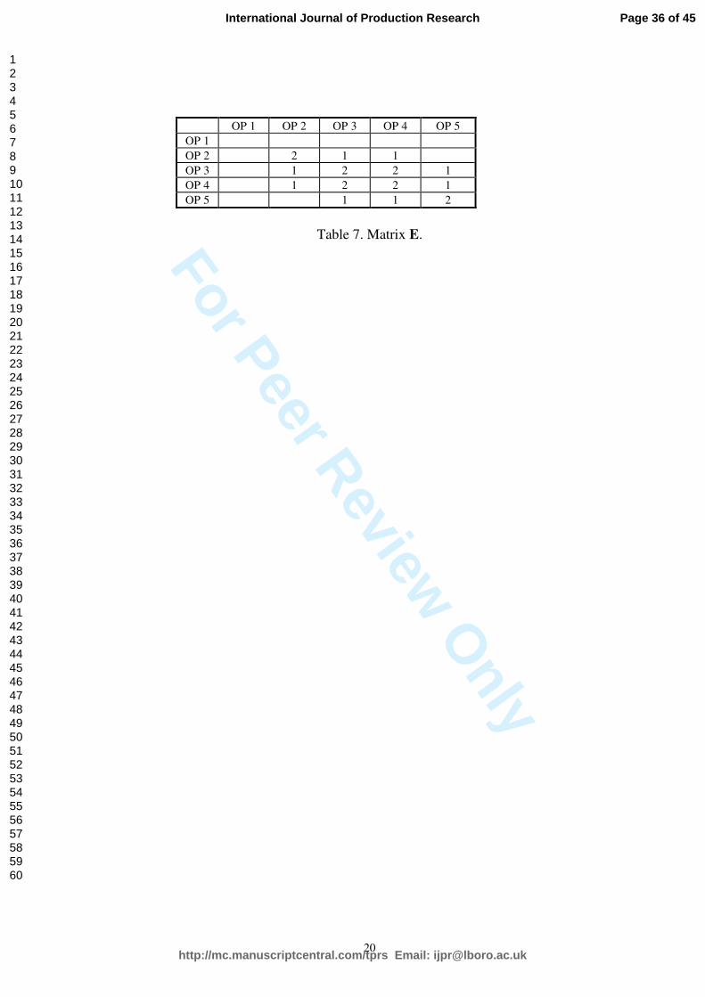
Table 7. Matrix E.

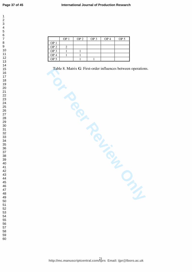
We can read here that operation 3 uses two characteristics for L/C and that operations 3 and 4 share two characteristics used for L/C (elements 3,3 and 3,4 of the Table). If we start now to study the direct and indirect influences between operations, we obtain the first-order influences in the matrix G:

B X’ = G In our example:

OP 1 OP 2 OP 3 OP 4 OP 5 OP 1 OP 2 2 OP 3 1 1 OP 4 1 1 OP 5 1 1

Table 8. Matrix G: First-order influences between operations.

Here we can identify that in operation 3 it has been used for L/C one characteristic that was changed in operation 1 and another one that was changed in operation 2 (elements 3,1 and 3,2 of the matrix). If we look for second-order influences, we make the product GG=K and obtain the matrix of Table 9.

OP 1 OP 2 OP 3 OP 4 OP 5 OP 1 OP 2 OP 3 2 OP 4 2 OP 5 3 1

Table 9. Matrix K: Second-order influences between operations.

In element 3,1 we read that operation 3 has been affected by operation 1 in two ways, by means of other operations. If we look at the previous tables, we find in Table 1 that in

Page 12 of 45



123456789101112131415161718192021222324252627282930313233343536373839404142434445464748495051525354555657585960

For Peer Review O

nly

13

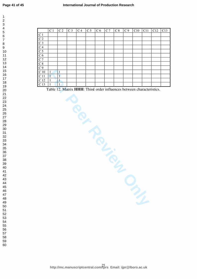
operation 1 characteristic 2 has been created, and that this characteristic is used for clamping in operation 2, where characteristic 3 is created. These two characteristics (2 and 3) are used for clamping and location in operation 3, and by these two ways, operation 1 is affecting operation 3, with one intermediate operation. Similar analysis can be made for the other elements of the table. To obtain third-order influences, we compute GGG, but this is now a null matrix, showing that there are no influences of third or upper-order between operations in this process. To study the relations between characteristics we can compute the matrix H, representing relations between characteristics:

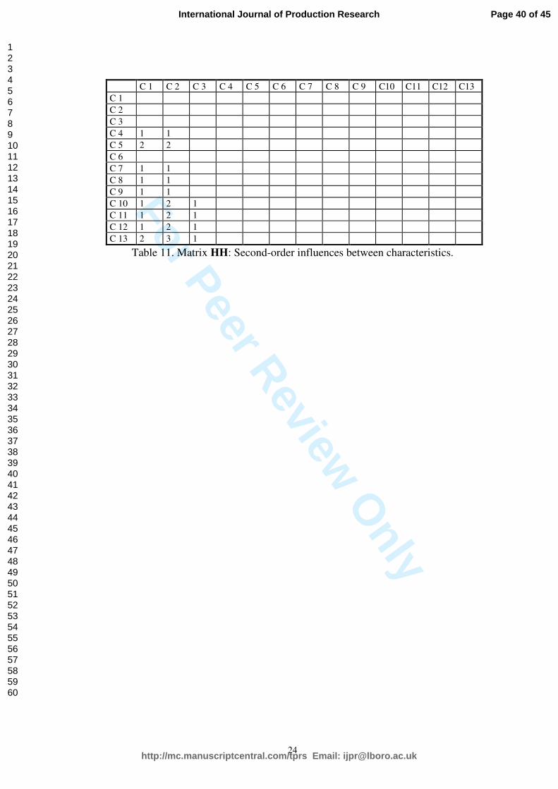
X’ B = H Representing the values of H the first-order influences (Table 10). We can calculate the second-order influences as HH (Table 11) and the third-order influences as HHH (Table 12). Influences or orders greater than three are zero. C 1 C 2 C 3 C 4 C 5 C 6 C 7 C 8 C 9 C10 C11 C12 C13 C 1 C 2 C 3 1 1 C 4 1 1 C 5 2 2 C 6 1 1 C 7 1 1 C 8 1 1 C 9 1 1 C 10 1 1 C 11 1 1 C 12 1 1 C 13 1 2 1

Table 10. Matrix H: First-order influences between characteristics. C 1 C 2 C 3 C 4 C 5 C 6 C 7 C 8 C 9 C10 C11 C12 C13 C 1 C 2 C 3 C 4 1 1 C 5 2 2 C 6 C 7 1 1 C 8 1 1 C 9 1 1 C 10 1 2 1 C 11 1 2 1 C 12 1 2 1 C 13 2 3 1

Table 11. Matrix HH: Second-order influences between characteristics.

Page 13 of 45



123456789101112131415161718192021222324252627282930313233343536373839404142434445464748495051525354555657585960

For Peer Review O

nly

14

C 1 C 2 C 3 C 4 C 5 C 6 C 7 C 8 C 9 C10 C11 C12 C13 C 1 C 2 C 3 C 4 C 5 C 6 C 7 C 8 C 9 C 10 1 1 C 11 1 1 C 12 1 1 C 13 1 1

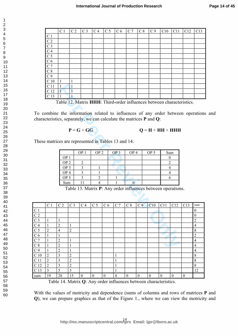
Table 12. Matrix HHH: Third-order influences between characteristics. To combine the information related to influences of any order between operations and characteristics, separately, we can calculate the matrices P and Q:

P = G + GG Q = H + HH + HHH These matrices are represented in Tables 13 and 14.

OP 1 OP 2 OP 3 OP 4 OP 5 Sum OP 1 0 OP 2 2 2 OP 3 3 1 4 OP 4 3 1 4 OP 5 3 2 1 6 Sum 11 4 1 0

Table 13. Matrix P: Any order influences between operations. C 1 C 2 C 3 C 4 C 5 C 6 C 7 C 8 C 9 C10 C11 C12 C13 sum C 1 0 C 2 0 C 3 1 1 2 C 4 1 2 1 4 C 5 2 4 2 8 C 6 1 1 2 C 7 1 2 1 4 C 8 1 2 1 4 C 9 1 2 1 4 C 10 2 3 2 1 8 C 11 2 3 2 1 8 C 12 2 3 2 1 8 C 13 3 5 3 1 12 sum 19 28 15 0 0 0 4 0 0 0 0 0 0 Table 14. Matrix Q: Any order influences between characteristics. With the values of motricity and dependence (sums of columns and rows of matrices P and Q), we can prepare graphics as that of the Figure 1., where we can view the motricity and

Page 14 of 45



123456789101112131415161718192021222324252627282930313233343536373839404142434445464748495051525354555657585960

For Peer Review O

nly

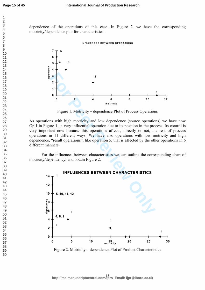
15

dependence of the operations of this case. In Figure 2. we have the corresponding motricity/dependence plot for characteristics.

IN F L U E N C E S B E TW E E N O P E R ATIO N S

0

1

2

3

4

5

6

7

0 2 4 6 8 10 12m o tric ity

depe

nden

cy

1

2

34

5

Figure 1. Motricity – dependence Plot of Process Operations

As operations with high motricity and low dependence (source operations) we have now Op.1 in Figure 1., a very influential operation due to its position in the process. Its control is very important now because this operations affects, directly or not, the rest of process operations in 11 different ways. We have also operations with low motricity and high dependence, “result operations”, like operation 5, that is affected by the other operations in 6 different manners. For the influences between characteristics we can outline the corresponding chart of motricity/dependency, and obtain Figure 2.

INFLUENCES BETWEEN CHARACTERISTICS

0

2

4

6

8

10

12

14

0 5 10 15 20 25 30motricity

depe

nden

cy

2

34, 8, 9

7

5, 10, 11, 12

6

1

Figure 2. Motricity – dependence Plot of Product Characteristics

Page 15 of 45



123456789101112131415161718192021222324252627282930313233343536373839404142434445464748495051525354555657585960

For Peer Review O

nly

16

Now we found characteristics 1, 2 and 3, characteristics with high motricity and low dependence, that have important influence over the others and, at the same time, receive only little influenced by the rest of the process (no influence in fact for characteristics 1 and 2). Specifically char. 2 affects the rest of characteristics in 28 different ways. Problems in any of these three characteristics tend to move along the process affecting other characteristics. We have also characteristics with low motricity and high dependence, as characteristics 13, 5, 10, 11 or 12, highly influenced by other product characteristics and usually difficult to control: characteristic 13 receives 12 different influences.

Acknowledgements We would like to thank the Foreign Language Co-ordination Office at the Polytechnic University of Valencia for their help in revising this paper. References. Carrión, A.; Jabaloyes J. “La matriz de características en control de calidad”. Actas del XXIII Congreso Nacional de Estadistica e Investigación Operativa. Sevilla, 1995 Ford Motor Company, División T&C. “Dimensional Control Plans. DCP Manual”. 1985 APQP-2 Advanced Product Quality Planning & Control Plan (APQP). AIAG. Second Printing February 1995. Duperrin, J.C.; Godet, M. “Methode de hierarchisation des elements d’un systeme”. Rapport Economique du CEA, R. 45.41 (1974). Godet, M. Prospectiva y Planificación estratégica. S.G. Editores, Barcelona 1991.

Page 16 of 45



123456789101112131415161718192021222324252627282930313233343536373839404142434445464748495051525354555657585960

For Peer Review O

nly

THE CHARACTERISTICS MATRIX AS A TOOL FOR ANALYSING PROCESS STRUCTURE

Andrés CarriónA1†*, José Jabaloyes A1* and Aura López A2*

A1Polytechnic University of Valencia. Camino de Vera s/n, 46022 Valencia, Spain.A2Pontificia Universidad Javeriana, Calle 18 No. 118-250 Av. Cañasgordas, Cali (Colombia).

ABSTRACTThe characteristics matrix is a tool to describe the relationship between product characteristics and process operations. It has been used traditionally with only descriptive purposes and analysed with a very limited intuitive approach. In this paper we present a methodology to analyse deeply the process structure using the information contained in the characteristics matrix. We apply the principles of the mic-mac method to study both direct and indirect internal relations, defining importance criteria and identifying the most important characteristics and operations.

Keywords: Quality; Mic-Mac Method; Process control; Process design; Characteristics Matrix

1. The role of the characteristics matrix in quality control.

Quality control in production processes requires the observation of some product characteristics, usually by means of control charts. With these charts we are able to monitor the evolution of the quality characteristic and detect the anomalous conditions that may arise.

However, there is an important stage, previous to the use of control charts, a less studied stage despite its great importance: the selection of the characteristics to control. Obviously, it is impossible to control all the product characteristics (dimensional, mechanical, electrical, …) therefore, it is necessary to select only a few of them. But the question is, which ones? The correct answer is obvious: the most important characteristics should be controlled. The question now is how to select these ‘important’ characteristics and how to measure their importance.

To do this, we have to take into account different aspects of the characteristics’ importance: importance for the product function, for the production process and for the customer. If we consider the first two elements, it is evident that we need a deep knowledge of the product and process at the moment of selecting the characteristics to control.

† Correspondence: acarrió[email protected] Postal address: Andrés Carrión. Departamento de Estadística e Investigación Operativa Aplicadas y Calidad. Universidad Politécnica de Valencia. Camino de Vera s/n 46022 –Valencia- Spain.• Dr Carrión is Director of the Department of Applied Statistics, O.R. and Quality of the Polytechnic

University of Valencia (Spain). He is member of the Spanish Society for Quality (AEC). acarrió[email protected]

• Dr Jabaloyes is Professor in the Department of Applied Statistics, O.R. and Quality of the Polytechnic University of Valencia (Spain). [email protected]

• Dr López is Professor of the Faculty of Engineering of the Pontificia Universidad Javeriana of Cali (Colombia). [email protected]

Page 17 of 45



123456789101112131415161718192021222324252627282930313233343536373839404142434445464748495051525354555657585960

For Peer Review O

nly

2

The characteristics matrix is a useful tool for this purpose. This matrix provides a fine and simple description of the production process and the effect that successive operations have on the product. The characteristics matrix (CM), usually a non square matrix, displays in rows the different process operations and in columns the product characteristics that are produced or used in the process operations. For example, in mechanization processes, most of the product characteristics are dimensional parameters. This matrix is used by different industrial procedures like Dimensional Control Plans (DCP), FMC (1985), and Advanced Product Quality Planning (APQP), AIAG (1995). Carrión and Jabaloyes (1995) presented a first study of the possibilities of this matrix for further analysis.

The general term of the CM, aij , is the kind of relations between the corresponding process operation (row i) and product characteristic (column j). Usually a set of symbols is used to represent this relation. The three most frequently used and most important are:

x characteristic created or modified in this operation.L characteristic used for locating the part.C characteristic used for clamping the part.

The use of that matrix is limited to its observation and to the intuitive evaluation of its contents, as it is like a map of the production process, and to the identification of the characteristics and more influential operations by simple inspection of the matrix. Table 1 in the example shows a simple example of such matrix.

The objective of this paper is to exploit the information contained in the characteristics matrix via a procedure based on the technological forecast mic-mac method (Duperrin and Godet, 1974; Godet 1991). In this method we consider a square matrix that places the variables affecting a certain system in rows and columns, and the matrix general term measures, in a subjective scale, the degree of influence among characteristics. Successive powers of that matrix permit to detect indirect relations among variables, that were not evident in the original matrix.

2. Study and analysis of the C.M.

Let’s consider a production process which includes m operations, and a product described by n quality characteristics. The characteristics matrix, as previously defined, will have m·n dimensions. For the study and analysis of the characteristics matrix, it is useful to separate the information of the matrix in two matrices with equal dimensions: the first one is called “changes matrix” and it contains the information related to the characteristics created or modified in each operation (corresponding to the code x of the traditional CM). The second one is called “LC matrix”, and it contains the information related to operations of locating and clamping (identified with the codes L and C in the traditional CM). In both matrices, the codes are substituted by 1 (one), remaining the rest of the terms in zero.

We will then have two matrices, usually of very low density, that collect the information on the process and the characteristics of the product. Operating with these matrices, we will obtain more information on the structure of the process and the relations between characteristics.

3. The matrix of changes.

Page 18 of 45



123456789101112131415161718192021222324252627282930313233343536373839404142434445464748495051525354555657585960

For Peer Review O

nly

3

First, let’s consider this matrix that collects the information of changes in product characteristics. If we call this changes matrix X, its general term xij is:

xij = 1 if characteristic j has been created or modified in the operation ixij = 0 in other cases

If we post-multiply it by its transposed X’, the result is a symmetric square matrix with m·m size (where m is the number of process operations):

X X’ = C

The general term for this matrix C, cij, is:

cij = ∑=

n

1kjkik xx

the values of cij represents:

• if i=j, cij is the number of characteristics created or modified in the operation i• if i≠j, cij is the number of common characteristics changed in both operations, i and

j.

We can also see that:


n

1jijc , is the number of changes that are produced

in the characteristics changed in that operation i, that is, the changes that are produced in the operation i plus the changes in other operations that affect the characteristics modified in operation i.

• The matrix trace C is the number of change actions that have been carried out in the process.

If we multiply now in the opposite order:

X’ X = D

We obtain the symmetric square matrix D, with n•n dimensions (where n is the number of product characteristics). The general element dij is:

dij = ∑=

m

1kkjki xx

the values of dij represent:

• if i=j, dij is the number of operations affecting the characteristic i• if i≠j, dij is the number of operations in which characteristics i and j are

simultaneously modified.

Page 19 of 45



123456789101112131415161718192021222324252627282930313233343536373839404142434445464748495051525354555657585960

For Peer Review O

nly

4

And we can also identify that:


m

1jijd , is the number of changes related to characteristic i,

produced in this characteristic or in any other characteristic and operation (that is: changes in characteristic i, plus changes in other characteristics that have changes simultaneously with i).

• As in C, the D matrix trace is the number of change actions performed in the process.

4. The LC Matrix.

If we call the LC Matrix B, we can work in the same way as with the Change Matrix X. If the general term of B, bij is:

bij = 1 if the characteristic j has been used for location or clamping (LC) in the operation ibij = 0 in other cases

If we post-multiply B by its transposed, we obtain a new symmetric square matrix E with m·m dimensions, where m is the number of operations in the process:

B B’ = E

The general term eij is:

eij = ∑=

n

1kjkik bb

the values of eij represent:

• if i=j, eij is the number of characteristics used for LC in operation i• if i≠j, eij is the number of common characteristics shared by operations i and j for

LC

Also, we can see that:


n

1jije , is the number of characteristics used for LC

actions that are related to operation i. That is, the LC actions carried out in the operation i plus the LC actions in other operations that use characteristics also used in operation i.

• The matrix trace E is the number of LC actions that have been carried out in the process.

If we pre-multiply B by its transposed:

B’ B = F

Page 20 of 45



123456789101112131415161718192021222324252627282930313233343536373839404142434445464748495051525354555657585960

For Peer Review O

nly

5

We obtain the matrix F, a symmetrical square matrix, with dimensions n•n (where n is the number of characteristics). The general term of F is:

fij = ∑=

m

1kkjkibb

the values of fij represent:

• if i=j, fij is the number of operations that use characteristic i for LC• if i≠j, fij is the number of operations in which characteristics i and j are

simultaneously used for LC.

And we can also identify that:


m

1jijf , is the number of LC actions related with the characteristic

i, referred to this characteristic or to any other characteristic acting together with characteristic i.

• The matrix trace F is the number of LC actions performed in the process.

5. Combination of the L/C and Changes Matrices.

The information previously obtained is interesting as it describes some non evident aspects of the production process structure, but is the joint use of both matrices what gives us the best results. In the following paragraphs we will present some of these results.

5.1. Influences between operations and between characteristics.

5.1.1 First-order influences.

A) First-order relationship between operations

If we post-multiply the L/C matrix by the transposed of the changes matrix:

B X’ = G

We obtain a non symmetric square matrix G, with as many rows and columns as operations in the process. The general term, gij ,is:

bij = ∑=

m

1kjkik xb

And we can find that:

• If i ≠ j, gij is the number of characteristics used for L/C in the operation i that were changed in the operation j. It establishes whether there is influence of operation j

Page 21 of 45



123456789101112131415161718192021222324252627282930313233343536373839404142434445464748495051525354555657585960

For Peer Review O

nly

6

on operation i, and, to a certain extent, the potential intensity of that influence (by the reiteration).

• If i = j, usually gij will be null, as it represents the number of times that a characteristic is employed for L/C is changed in that same operation.

The number of non zero elements of column j is the number of operations influenced by the operation j through L/C.

B) First-order relationship between characteristics

If we now pre-multiply the L/C matrix by the transposed of the changes matrix, we obtain a new non symmetric square matrix, H, with as many rows or columns as characteristics of the part under study.

X’ B = H

The general term hij is:

hij = ∑=

m

1kjkik bx

where:

• If i ≠ j, hij is the number of times that characteristic I is modified using characteristic j for L/C. It establishes whether there is influence of characteristic j on characteristic i, and, to a certain extent, the potential intensity of that influence (by the reiteration).

• If i = j, usually hij will be null

The number of non zero elements in column j represents the number of characteristics influenced by the characteristic j, via L/C.

5.1.2. Second-order influences.

A) Second-order relationship between operations

In the two previous cases, the influences identified are of first-order, in the sense that are direct influences of an operation (or characteristic) on another. We can be interested in the indirect influences.

If we take now the square matrix G and we multiply it by itself, we obtain a new matrix that collects the second-order influences of operation j on operation i, that is, influences between two operations with a third intermediate operations (e.g.: op1 influencing op2, and op2 influencing op3, and as a consequence, indirect influence of op1 on op3):

G G = K

Page 22 of 45



123456789101112131415161718192021222324252627282930313233343536373839404142434445464748495051525354555657585960

For Peer Review O

nly

7

Where the general term kij is the number of single intermediate influences of operation j on operation i.

B) Second-order relationship between characteristics

In a similar way, we can obtain:

H H = L

Where L is a square matrix with as many dimensions as characteristics, and whose general term lij is the number of second-order influences, that is, influences between two characteristics (characteristics j on characteristic i) with a third one as intermediate.

5.1.3. Upper-order influences.

We can obtain influences of third, fourth or upper-order simply by multiplying the appropriate number of times each of the matrices G and H; for the third-order influences between operations we have to calculate G G G, and for influences between characteristics H H H; for the fourth-order influences between operations we have to calculate G G G G, and for influences between characteristics H H H H; and so on.

At a certain point, depending on the complexity of process and product, those matrices will be null, indicating that there are no relations of that order, neither upper-order, among operations or characteristics. The highest order corresponds to the number of operations for one case and to the number of characteristics for the other.

5.1.3. Global influences evaluation.

If we sum these matrices obtained as successive power of G until obtaining the null matrix, we obtain:

P = G + G G + G G G + ...

Where P is a square matrix (dimensions m•m), that includes the relationships of any order between process operations:

• pij, if i ≠ j, is the number of direct or indirect influences of operation j on operation i.

• pij, if i = j, is zero.• ∑

jijp = number of influences, direct or indirect, affecting operation i.

• ∑i

ijp = number of influences, direct or indirect, generated by operation j.

In the same way, we can evaluate relations among characteristics obtaining:

Q = H + H H + H H H + ...

where Q is a square matrix (dimensions n•n) whose general element is:

Page 23 of 45



123456789101112131415161718192021222324252627282930313233343536373839404142434445464748495051525354555657585960

For Peer Review O

nly

8

• qij, if i ≠ j, is the number of direct or indirect influence ways of characteristic j on characteristic i.

• qij, si i = j, is zero.• ∑

jijq = number of influences, direct or indirect, affecting characteristic i.

• ∑i

ijq = number of influences, direct or indirect, generated by characteristic j.

6. Influence chart.

In the mic-mac method the concepts of motricity and dependence are defined and used. The first one refers to the degree of influence that one variable has over the others. The dependence is the degree to which one variable is influenced by the others. The same idea can be used here, referred both to process operations and to product characteristics. The motricity will be the sum by columns and the dependence the sum by rows of the corresponding matrices P and Q.

If we consider the matrix P, relations between operations, we have that

pijj∑

is the number of influences received by the operation i from all the other operations, that is, its dependence. Also in matrix P, we have that

piji∑

is the number of influences generated by the operation j, that is its motricity.

The same operations can be done in matrix Q, obtaining in this way the dependence and motricity for each characteristic.

With these pairs of data, we can prepare an XY plot, having in x-axis the motricity and in y-axis the dependence. This graphic is a plot of the nature of the inter-operations (or inter-characteristics) relationships in the process.

Operations with high motricity and low dependence are the operation with higher influence over the others and, at the same time, less influenced by others. Usually this kind of operations will be at the beginning of the process. Its control is very important due to its great influence over subsequent operations and, in general, over the process. We can understand these as “source operations”. In the opposite corner, we have operations with low motricity and high dependence. These can be called “result operations”, very influenced by the rest of the process and usually difficult to control.

Page 24 of 45



123456789101112131415161718192021222324252627282930313233343536373839404142434445464748495051525354555657585960

For Peer Review O

nly

9

For the influences between characteristics we can also outline the corresponding motricity/dependence plot. As in the previous chart, characteristics with high motricity and low dependence are those with important influence over the others, but, on the other hand, not influenced by the rest of the process. These can be called “source characteristics”. Quality problems in one of these characteristics tend to move along the process affecting other characteristics. In the opposite situations we have characteristics with low motricity and high dependence, highly influenced by other product characteristics and usually difficult to control. We can name these as “result characteristics”.

7. Conclusions.

The analysis of the characteristics matrix has proven to provide important information about the process, the internal relationship structure between operations and between characteristics. In this way, this matrix is an interesting procedure to study and understand this complex relationship structure.

With its help, and with simple operations we can distinguish the most influential operations and characteristics, and use this information to carefully control these activities, as any problem that appears here will spread over the process, affecting other operations and characteristics. We can also identify other operations or characteristics that will be, in advance, difficult to control, as they are the effect of many sources of variation. Control on these operations or characteristics needs to take into account that in many cases problem solving need to focus on operations or characteristics different to the places where the problem has been detected.

8. Example

The case defined in Table 1 is a simple example of the application of the procedure described before to a mechanising process.

[Insert Table 1 about here]

This process can be described, basing on Table 1, as follows:

1. In Operation 1 we receive raw parts with characteristics C.1 and C.22. In Op. 2 characteristic C.1 is used for locating, C.2 is used for clamping and

characteristics C.3 and C.6 are created.3. In Op. 3 characteristic C.2 is used again for clamping, C.3 for locating and

characteristics C.4, C.5 and C.7 are created or modified.4. In Op. 4 again C.2 is used for clamping and C.3 for locating, and C.5, C.8, C.9 and

C.13 are created or modified.5. Finally, in Op. 5 characteristic C.3 is used for locating, C.7 for clamping and

characteristics C.10, C.11, C.12 and C.13 are created or modified.

Page 25 of 45



123456789101112131415161718192021222324252627282930313233343536373839404142434445464748495051525354555657585960

For Peer Review O

nly

10

With this table we can build the two matrices that we have called “matrix of changes” and “L/C matrix”. The changes matrix is represented in Table 2. and L/C matrix in Table 3.:



Working with the changes matrix X, and to study the relations between operations we will compute the product XX’, obtaining the square matrix C, shown in Table 4.


We can see here that, for instance:• in Operation 2 there have been changed (created or modified) two characteristics

(element 2,2 of the matrix): in Table 1 we can confirm that this two characteristics are C.3 and C.6.

• in Operation 5 four characteristics have been changed (element 5,5 of the matrix): in Table 1 we can see that these characteristics are C.10, C.11, C.12 and C.13.

• We can read that there is one common characteristic changed in operations 3 and 4 (element 4,3 or 3,4 of the matrix): in Table 1 we verify that this characteristic is C.5, that was created in operation 3 and modified in operation 4.

If we change the order of the product that we have made to obtain matrix C, we will have matrix D = X’X, presented in Table 5.:


In Table 5 zeroes have been omitted for easier reading of the table. These criteria will be used from now on.

As examples, we can see in Table 5 that:• Characteristic 3 is affected by only one operation (element 3,3 of the matrix): In

Table 1 we read that this operation is Op. 2. • Characteristic 5 is affected by two operations (element 5,5 of the matrix): In Table 1

we read that these two operations are Op. 3 and Op. 4.• If we have a look outside the diagonal, we find that characteristics 6 and 3 have

changed together in one operation (element 3,6 of the matrix): In table 1 we read that this operations is Op. 2. It also occurs with many others as characteristics 1 and 2 or 11 and 12 (elements 1,2 and 11,12 of the matrix).

Working now with the L/C matrix, we can obtain matrices F and G from:

B’B = F B B’ = E

In Tables 6 and 7 we present these matrices for the case studied as example:

Page 26 of 45



123456789101112131415161718192021222324252627282930313233343536373839404142434445464748495051525354555657585960

For Peer Review O

nly

11


We find here that characteristic 2 has been used for L/C (location or clamping) three times, and that characteristics 2 and 3 have been used together for L/C twice (elements 2,2 and 2,3 of the table).


We can read here that operation 3 uses two characteristics for L/C and that operations 3 and 4 share two characteristics used for L/C (elements 3,3 and 3,4 of the Table).

If we start now to study the direct and indirect influences between operations, we obtain the first-order influences in the matrix G:

B X’ = GIn our example:


Here we can identify that in operation 3 it has been used for L/C one characteristic that was changed in operation 1 and another one that was changed in operation 2 (elements 3,1 and 3,2 of the matrix).

If we look for second-order influences, we make the product GG=K and obtain the matrix of Table 9.


In element 3,1 we read that operation 3 has been affected by operation 1 in two ways, by means of other operations. If we look at the previous tables, we find in Table 1 that in operation 1 characteristic 2 has been created, and that this characteristic is used for clamping in operation 2, where characteristic 3 is created. These two characteristics (2 and 3) are used for clamping and location in operation 3, and by these two ways, operation 1 is affecting operation 3, with one intermediate operation. Similar analysis can be made for the other elements of the table.

To obtain third-order influences, we compute GGG, but this is now a null matrix, showing that there are no influences of third or upper-order between operations in this process.

To study the relations between characteristics we can compute the matrix H, representing relations between characteristics:

X’ B = H

Representing the values of H the first-order influences (Table 10). We can calculate the second-order influences as HH (Table 11) and the third-order influences as HHH (Table 12). Influences or orders greater than three are zero.

Page 27 of 45



123456789101112131415161718192021222324252627282930313233343536373839404142434445464748495051525354555657585960

For Peer Review O

nly

12




To combine the information related to influences of any order between operations and characteristics, separately, we can calculate the matrices P and Q:

P = G + GG Q = H + HH + HHH

These matrices are represented in Tables 13 and 14.



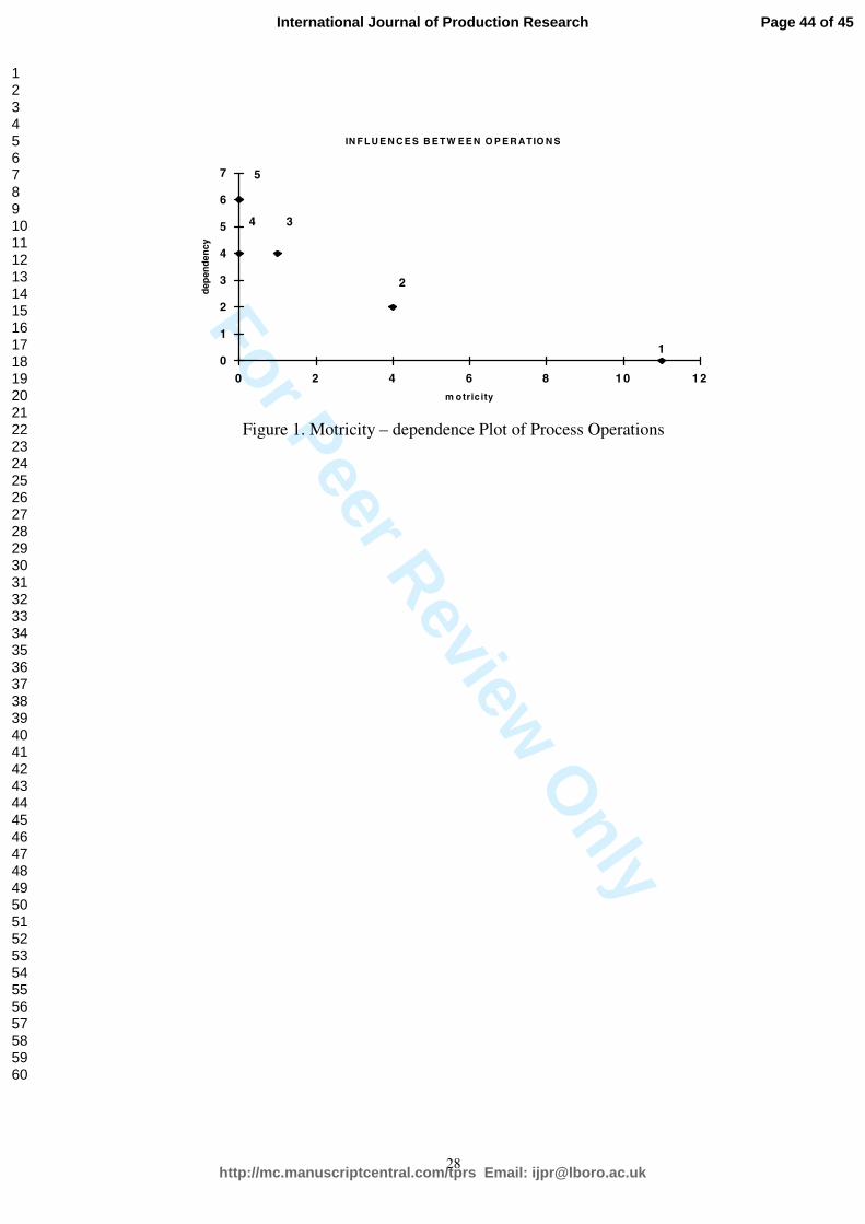
With the values of motricity and dependence (sums of columns and rows of matrices P and Q), we can prepare graphics as that of the Figure 1., where we can view the motricity and dependence of the operations of this case. In Figure 2. we have the corresponding motricity/dependence plot for characteristics.

[Insert Figure 1 about here]

As operations with high motricity and low dependence (source operations) we have now Op.1 in Figure 1., a very influential operation due to its position in the process. Its control is very important now because this operations affects, directly or not, the rest of process operations in 11 different ways. We have also operations with low motricity and high dependence, “result operations”, like operation 5, that is affected by the other operations in 6 different manners.

For the influences between characteristics we can outline the corresponding chart of motricity/dependency, and obtain Figure 2.

[Insert Figure 2 about here]

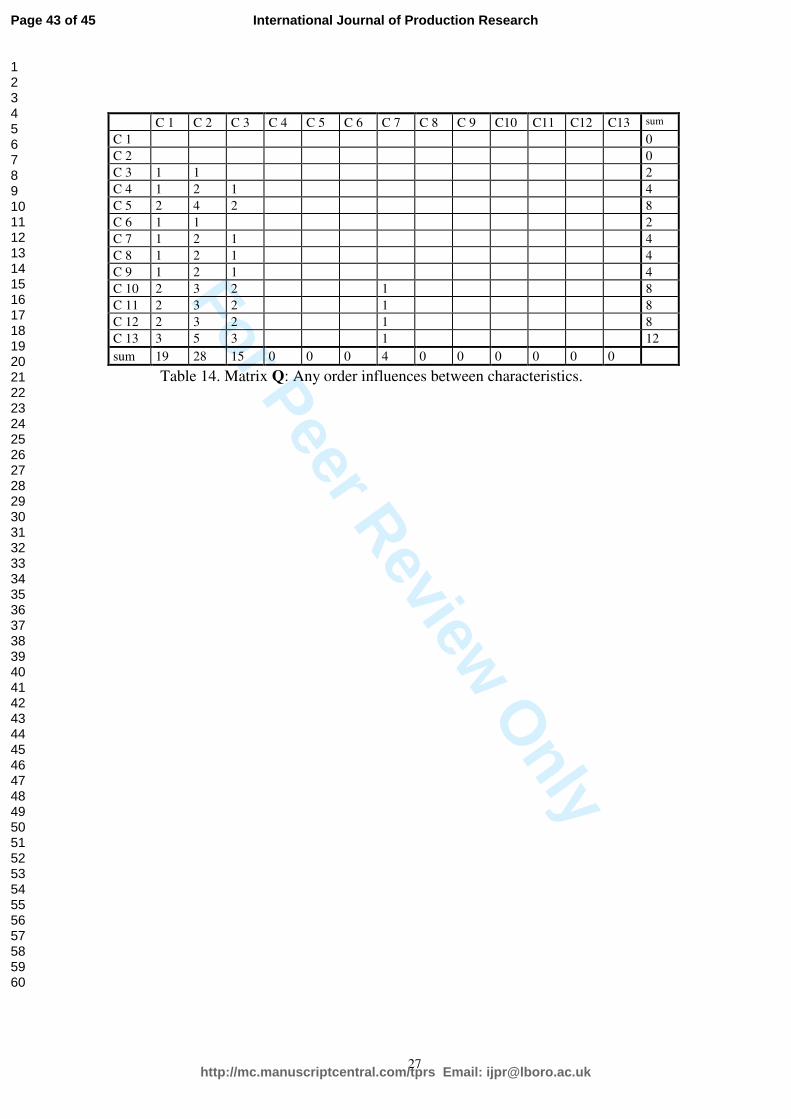
Now we found characteristics 1, 2 and 3, characteristics with high motricity and low dependence, that have important influence over the others and, at the same time, receive only little influenced by the rest of the process (no influence in fact for characteristics 1 and 2). Specifically char. 2 affects the rest of characteristics in 28 different ways. Problems in any of these three characteristics tend to move along the process affecting other characteristics. We have also characteristics with low motricity and high dependence, as characteristics 13, 5, 10, 11 or 12, highly influenced by other product characteristics and usually difficult to control: characteristic 13 receives 12 different influences.

Acknowledgements

Page 28 of 45



123456789101112131415161718192021222324252627282930313233343536373839404142434445464748495051525354555657585960

For Peer Review O

nly

13

We would like to thank the Foreign Language Co-ordination Office at the Polytechnic University of Valencia for their help in revising this paper.

References.

Carrión, A.; Jabaloyes J. “La matriz de características en control de calidad”. Actas del XXIII Congreso Nacional de Estadistica e Investigación Operativa. Sevilla, 1995

Ford Motor Company, División T&C. “Dimensional Control Plans. DCP Manual”. 1985

APQP-2 Advanced Product Quality Planning & Control Plan (APQP). AIAG. Second Printing February 1995.

Duperrin, J.C.; Godet, M. “Methode de hierarchisation des elements d’un systeme”. Rapport Economique du CEA, R. 45.41 (1974).

Godet, M. Prospectiva y Planificación estratégica. S.G. Editores, Barcelona 1991.

Page 29 of 45



123456789101112131415161718192021222324252627282930313233343536373839404142434445464748495051525354555657585960

For Peer Review O

nly

14

C.1 C.2 C.3 C.4 C.5 C.6 C.7 C.8 C.9 C.10 C.11 C.12 C.13OP.1 X XOP.2 L C X XOP.3 C L X X XOP.4 C L X X X XOP.5 L C X X X X

Table 1. Characteristic Matrix of a simple process.

Page 30 of 45



123456789101112131415161718192021222324252627282930313233343536373839404142434445464748495051525354555657585960

For Peer Review O

nly

15

C.1 C.2 C.3 C.4 C.5 C.6 C.7 C.8 C.9 C.10 C.11 C.12 C.13OP.1 1 1 0 0 0 0 0 0 0 0 0 0 0OP.2 0 0 1 0 0 1 0 0 0 0 0 0 0OP.3 0 0 0 1 1 0 1 0 0 0 0 0 0OP.4 0 0 0 0 1 0 0 1 1 0 0 0 1OP.5 0 0 0 0 0 0 0 0 0 1 1 1 1

Table 2. Changes Matrix X. Characteristics creation or modification

Page 31 of 45



123456789101112131415161718192021222324252627282930313233343536373839404142434445464748495051525354555657585960

For Peer Review O

nly

16

C.1 C.2 C.3 C.4 C.5 C.6 C.7 C.8 C.9 C.10 C.11 C.12 C.13OP.1 0 0 0 0 0 0 0 0 0 0 0 0 0OP.2 1 1 0 0 0 0 0 0 0 0 0 0 0OP.3 0 1 1 0 0 0 0 0 0 0 0 0 0OP.4 0 1 1 0 0 0 0 0 0 0 0 0 0OP.5 0 0 1 0 0 0 1 0 0 0 0 0 0

Table 3. L/C Matrix B. Location and clamping characteristics

Page 32 of 45



123456789101112131415161718192021222324252627282930313233343536373839404142434445464748495051525354555657585960

For Peer Review O

nly

17

OP 1 OP 2 OP 3 OP 4 OP 5OP 1 2 0 0 0 0OP 2 0 2 0 0 0OP 3 0 0 3 1 0OP 4 0 0 1 4 1OP 5 0 0 0 1 4

Table 4. Matrix C.

Page 33 of 45



123456789101112131415161718192021222324252627282930313233343536373839404142434445464748495051525354555657585960

For Peer Review O

nly

18

C 1 C 2 C 3 C 4 C 5 C 6 C 7 C 8 C 9 C10 C11 C12 C13C 1 1 1C 2 1 1C 3 1 1C 4 1 1 1C 5 1 2 1 1 1 1C 6 1 1C 7 1 1 1C 8 1 1 1 1C 9 1 1 1 1C 10 1 1 1 1C 11 1 1 1 1C 12 1 1 1 1C 13 1 1 1 1 1 1 2

Table 5. Matrix D.

Page 34 of 45



123456789101112131415161718192021222324252627282930313233343536373839404142434445464748495051525354555657585960

For Peer Review O

nly

19

C 1 C 2 C 3 C 4 C 5 C 6 C 7 C 8 C 9 C10 C11 C12 C13C 1 1 1C 2 1 3 2C 3 2 3 1C 4C 5C 6C 7 1 1C 8C 9C 10C 11C 12C 13

Table 6. Matrix F.

Page 35 of 45



123456789101112131415161718192021222324252627282930313233343536373839404142434445464748495051525354555657585960

For Peer Review O

nly

20

OP 1 OP 2 OP 3 OP 4 OP 5OP 1OP 2 2 1 1OP 3 1 2 2 1OP 4 1 2 2 1OP 5 1 1 2

Table 7. Matrix E.

Page 36 of 45



123456789101112131415161718192021222324252627282930313233343536373839404142434445464748495051525354555657585960

For Peer Review O

nly

21

OP 1 OP 2 OP 3 OP 4 OP 5OP 1OP 2 2OP 3 1 1OP 4 1 1OP 5 1 1

Table 8. Matrix G: First-order influences between operations.

Page 37 of 45



123456789101112131415161718192021222324252627282930313233343536373839404142434445464748495051525354555657585960

For Peer Review O

nly

22

OP 1 OP 2 OP 3 OP 4 OP 5OP 1OP 2OP 3 2OP 4 2OP 5 3 1

Table 9. Matrix K: Second-order influences between operations.

Page 38 of 45



123456789101112131415161718192021222324252627282930313233343536373839404142434445464748495051525354555657585960

For Peer Review O

nly

23

C 1 C 2 C 3 C 4 C 5 C 6 C 7 C 8 C 9 C10 C11 C12 C13C 1C 2C 3 1 1C 4 1 1C 5 2 2C 6 1 1C 7 1 1C 8 1 1C 9 1 1C 10 1 1C 11 1 1C 12 1 1C 13 1 2 1

Table 10. Matrix H: First-order influences between characteristics.

Page 39 of 45



123456789101112131415161718192021222324252627282930313233343536373839404142434445464748495051525354555657585960

For Peer Review O

nly

24

C 1 C 2 C 3 C 4 C 5 C 6 C 7 C 8 C 9 C10 C11 C12 C13C 1C 2C 3C 4 1 1C 5 2 2C 6C 7 1 1C 8 1 1C 9 1 1C 10 1 2 1C 11 1 2 1C 12 1 2 1C 13 2 3 1

Table 11. Matrix HH: Second-order influences between characteristics.

Page 40 of 45



123456789101112131415161718192021222324252627282930313233343536373839404142434445464748495051525354555657585960

For Peer Review O

nly

25

C 1 C 2 C 3 C 4 C 5 C 6 C 7 C 8 C 9 C10 C11 C12 C13C 1C 2C 3C 4C 5C 6C 7C 8C 9C 10 1 1C 11 1 1C 12 1 1C 13 1 1

Table 12. Matrix HHH: Third- order influences between characteristics.

Page 41 of 45



123456789101112131415161718192021222324252627282930313233343536373839404142434445464748495051525354555657585960

For Peer Review O

nly

26

OP 1 OP 2 OP 3 OP 4 OP 5 SumOP 1 0OP 2 2 2OP 3 3 1 4OP 4 3 1 4OP 5 3 2 1 6Sum 11 4 1 0

Table 13. Matrix P: Any order influences between operations.

Page 42 of 45



123456789101112131415161718192021222324252627282930313233343536373839404142434445464748495051525354555657585960

For Peer Review O

nly

27

C 1 C 2 C 3 C 4 C 5 C 6 C 7 C 8 C 9 C10 C11 C12 C13 sum

C 1 0C 2 0C 3 1 1 2C 4 1 2 1 4C 5 2 4 2 8C 6 1 1 2C 7 1 2 1 4C 8 1 2 1 4C 9 1 2 1 4C 10 2 3 2 1 8C 11 2 3 2 1 8C 12 2 3 2 1 8C 13 3 5 3 1 12sum 19 28 15 0 0 0 4 0 0 0 0 0 0

Table 14. Matrix Q: Any order influences between characteristics.

Page 43 of 45



123456789101112131415161718192021222324252627282930313233343536373839404142434445464748495051525354555657585960

For Peer Review O

nly

28

IN F L U E N C E S B E TW E E N O P E R ATIO N S

0

1

2

3

4

5

6

7

0 2 4 6 8 10 12

m otric ity

dep

end

ency

1

2

34

5

Figure 1. Motricity – dependence Plot of Process Operations

Page 44 of 45



123456789101112131415161718192021222324252627282930313233343536373839404142434445464748495051525354555657585960

For Peer Review O

nly

29

INFLUENCES BETWEEN CHARACTERISTICS

0

2

4

6

8

10

12

14

0 5 10 15 20 25 30motricity

dep

end

ency

2

34, 8, 9

7

5, 10, 11, 12

6

1

Figure 2. Motricity – dependence Plot of Product Characteristics

Page 45 of 45



123456789101112131415161718192021222324252627282930313233343536373839404142434445464748495051525354555657585960

Documents

THE CHARACTERISTICS MATRIX AS A TOOL FOR ANALYSING …