Embed Size (px)
Citation preview
BarcelonaEconomicsWorkingPaperSeries
WorkingPapernº376
“The Child is Father of the Man:” Implications for the Demographic
Transition
David de la Croix
Omar Licandro
‘The Child is Father of the Man:’
Implications for the Demographic Transition
David de la CroixDepartment of Economics and CORE, Universite catholique de Louvain
Omar Licandro
European University Institute and CEPR
March 10, 2009
Abstract
We propose a new theory of the demographic transition based on the evidencethat body development during childhood is an important predictor of adult life ex-pectancy. This theory is embodied in an OLG framework where fertility, longevityand education all result from individual decisions. The model displays differentregimes, allowing the economy to move slowly from an initial Malthusian regimetowards the Modern era. The dynamics reproduces the key features of the demo-graphic transition, including the permanent increase in life expectancy, resultingfrom improvements in body development, the hump in both population growthand fertility, and a late increase in secondary educational attainments.
JEL Classification Numbers: J11, I12, N30, I20, J24.Keywords: Life Expectancy, Height, Education, Fertility, Mortality.
1De la Croix acknowledges the financial support of the Belgian French speaking community (GrantARC 03/08-235 “New Macroeconomic Approaches to the Development Problem”) and the Belgian Fed-eral Government (Grant PAI P6/07 “Economic Policy and Finance in the Global Economy: EquilibriumAnalysis and Social Evaluation”). Licandro acknowledges the financial support of the Spanish Ministryof Education (SEJ2004-0459/ECON and SEJ2007-65552) and the Catedra Sabadell. We thank JoergBaten and Richard Steckel for making their data available to us. Matteo Cervellati, Juan Carlos Cor-doba, Nezih Guner, Moshe Hazan, Sebnem Kalemli-Ozcan, Omer Moav, Ruben Segura-Cayuela, DavidWeil, Hosny Zoabi and participants to seminars in Amsterdam, CER-ETH (Zurich), Bologna, Copen-hagen, Hebrew U. (Jerusalem), Humboldt (Berlin), IAE (Barcelona), IGIER (Milan), Marseille, ParisNsnterre, Paris School of Economics, Bank of Spain, Southampton, ULB (Brussels), Vienna, workshopsin ITAM (Mexico), IZA (Bonn) and CREI (Barcelona) and conferences SED 07, PET 08, ASSET 08,SEA 08, and ASSA 09 gave very useful comments on earlier drafts.

1 Introduction
Providing children with appropriate hygienic conditions and good nutrition, as well as a
good attitude towards health during childhood, are very effective ways of affording them
a longer life. Starting with Kermack, McKendrick, and McKinlay (1934), who showed
that the first fifteen years of life were central in determining the longevity of the adult,
the relationship between early development and late mortality has been well-established.
Fogel (1994) emphases that nutrition and physiological status are at the basis of the link
between childhood development and longevity. Another important mechanism stressed
by epidemiologists links infections and related inflammations during childhood to the
appearance of specific diseases in old age (Crimmins and Finch 2006). In the same
direction, Barker and Osmond (1986) relates lower childhood health status to higher
incidence of heart disease in later life. It is in this sense that, following Harris (2001),
we echo Wordsworth (1802)’s aphorism “The Child is Father of the Man,” meaning that
the way a child is brought up determines what she or he will become in the future.1
It is well documented that the timing of fertility, mortality and education differ during
the demographic transition. We illustrate it for Sweden in Section 2. First, body devel-
opment and adult life expectancy have both permanently improved from the beginning
of the 19th century. Second, the time profile of net fertility rates, net of infant mortal-
ity, is hump shaped, declining from the dawn of the 20th century. As it is well known,
the combination of these two forces made population growth rates also hump shaped.
Finally, years of schooling that start increasing around 1850, accelerate at the beginning
of the 20th century with the development of secondary education.
In this paper, we propose a new theory of the demographic transition based on the cited
evidence that body development during childhood favors adult longevity. We claim
the demographic transition have been shaped by a slow but permanent improvement
in childhood development, promoting adult life expectancy. As pointed out by (Galor
2005a) “The reversal in the fertility patterns in England ... suggests therefore that the
1The state of the debate between nature and nurture may be synthesized by the following statement“The effects of genes depend on the environment,” (Pinker 2004) where genes are associated with nature,and the environment, as a short-hand for the effects of human behavior, with nurture. In this paper, weare mainly interested in understanding how changes in human behavior, for a given distribution of genes,affect childhood development and then demographics. By restricting the analysis to a representativecohort member, a standard assumption in OLG models, we do not pay much attention to within cohortdifferences in genes, but concentrate on how changes in nurture over time affect childhood developmenton average. The implicit assumption is that the complex interaction between nature and nurture shapingthe distribution of childhood development across cohort members in society has no significant effect onthe mean over a period of time covering some few centuries.
2

demographic transition was prompted by a different universal force than the decline
in infant and child mortality.” In our view, contrary to reductions in infant and child
mortality, deliberate improvements in childhood development promoting adult survival
have prompted the demographic transition, in particular the observed fertility patterns.
When today’s developed world was in the Malthusian era, most individuals were liv-
ing at the subsistence level. Small changes in the environment inducing improvements
in adult life expectancy slowly increased individual’s lifetime surplus, allowing people
to afford more and healthy descendants, which reinforced the initial effect of an im-
proved environment on survival. As a consequence, net fertility rates were increasing
as predicted by the Malthusian theory. At some point at the beginning of the 19th
century, the Western world escaped the subsistence trap and the desire of having more
children became dominated by the search of an individual better life. Net fertility rates
remained high but stable for some decades while life expectancy kept growing. Finally,
with the arrival of the 20th Century, for the first time in human history adults started
finding it attractive to invest in their own human capital, which reduced the incentives
to have children and, consequently, net fertility rates. More educated, richer cohorts
have additional incentives to invest in childhood development, keeping life expectancy
permanently growing up to our days.
The model in this paper is a continuous time overlapping generations economy as in
Boucekkine, de la Croix, and Licandro (2002), where the key demographic variables,
fertility, mortality and education, are all decided by individuals. Parents like to have
children, but they also care about child longevity. By ensuring an appropriate physical
development for their children, parents provide them with a longer life. Such provision is
costly though, and its cost is increasing with the number of children. As a consequence,
having many children prevents parents of spending much on their body development,
which makes longevity and fertility negatively related in the modern era.2 We assume
adults decide about their own education, and we take basic education, even if provided
by parents, as being exogenously given. Adults face a trade-off between having children
2We are aware that longevity does not depend solely on childhood development. Adults’ investmentin health and government spending on the elderly also contribute considerably to reductions in mortality.However, adding these mechanisms into our setup would not alter the trade-off we want to put forward,and, therefore, we abstract from them in order to streamline the argument. We are also aware thatthere are at least two different types of health capital, as pointed out by Murphy and Topel (2006).One extends life expectancy so that individuals can enjoy consumption and leisure for longer; the otherincreases the quality of life, raising utility from a given quantity of consumption and leisure. In thispaper, since we are mainly interested in longevity, we restrict the analysis to the first type of healthcapital.
3

and improving their own education, which makes the number of children and schooling
negatively related. This is similar to the trade-off faced by parents in a Beckerian
world, where they care about the quantity and quality (education) of their offsprings.
However, observed data on primary school education anticipate in many decades the
decline in fertility predicted by the Beckerian theory, but not secondary school, as shown
by Figure 1. Finally, the mechanism relating demographics and education is the Ben-
Porath hypothesis that longevity positively affects education, by extending individual
active life.3
The model dynamics displays the key features of the demographic transition, including
the observed permanent rise in adult life expectancy, the hump in net fertility and the
late increase in secondary educational attainments. For this reason, we claim that body
development and adult life expectancy played a fundamental role explaining the demo-
graphic transformations faced by Western economies. In particular, it has promoted an
initial increase in fertility, with improvements on secondary education and reductions in
fertility arriving late with the modern era at the beginning of the 20th century.4
This article differs from the previous attempts in the literature to endogenize fertility and
longevity. Many papers have the standard education/fertility trade-off with exogenous
longevity, for example Doepke (2004) and Soares (2005). Other papers model health
investment either by households (Chakraborty and Das (2005) and Sanso and Aisa
(2006)) or by the government (Chakraborty (2004) and Aisa and Pueyo (2006)) but have
exogenous fertility. A few treat both fertility and longevity as endogenous variables, but
the mechanism leading to longer lives always relies on an externality: more aggregate
human capital or more aggregate income leads to higher life expectancy (Blackburn and
Cipriani (2002), Kalemli-Ozcan (2002), Lagerloef (2003), Cervellati and Sunde (2005)
and (2007) and Hazan and Zoabi (2006)).
Two recent papers have modeled the trade-off between the number and survival of
children exclusively in the context of pre-modern societies. In Galor and Moav (2005)’s
paper, there is an evolutionary trade-off (i.e. not faced by individuals but by nature),
between the survival to adulthood of each offspring and the number of offspring that can
be supported. Lagerloef (2007) suggested that agents chose how aggressively to behave,
given that less aggressive agents stand a better chance of surviving long enough to have
3Conditions for this mechanism to hold in the presence of endogenous fertility are derived in Hazanand Zoabi (2006). The main argument in our paper would also hold if, as in Hazan and Zoabi, childhooddevelopment affects education directly because healthier children perform better.
4The role of life expectancy on raising income well before the industrial revolution has been stressedby Boucekkine, de la Croix, and Licandro (2003).
4
children, but gain less resources, so more of their children die early from starvation. In
both cases, the trade-off is between the number and survival of children, while in our
paper it is between the number of children and adult longevity.
This paper is organized as follows. Section 2 presents some evidence on the link between
the improvement in childhood development and the demographic transition. In Sec-
tion 3.1, we present and solve the problem for individuals. Section 3.2 is devoted to the
study of the dynamics of dynasties. The demographic transition is analyzed in Section 4.
Implications for growth are studied in Section 5. Section 6 presents our conclusions.
2 Childhood Development and Demographic
Transition
Height at age 18 is a good measure of childhood development, since both better nutrition
and lower exposure to infections leads to increased height, and a good predictor of adult
life expectancy.5 According to Waaler (1984), the trend towards greater height found in
the data means that younger cohorts, which have grown up under better conditions, de-
velop more and live longer as adults. Height is also frequently used as a health indicator
in microeconomic studies. Weil (2007) finds that the effect on wages of an additional
centimeter of height ranges between 3.3% and 9.4%. In a second step, he exploits the
correlation between height and direct measures of health such as the adult survival rate
to evaluate health’s role in accounting for income differences among countries; he finds
that eliminating health variations would reduce world income variance by a third.
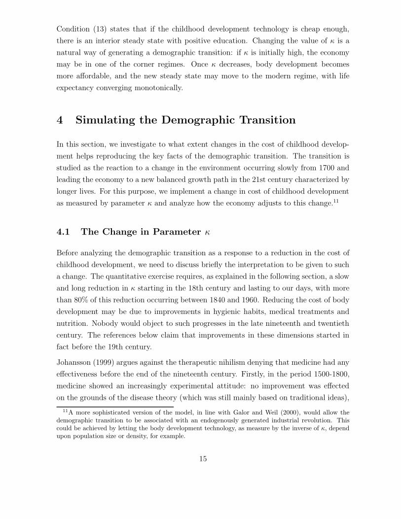
The height of conscripts has been systematically recorded by the Swedish army since
1820, which provides a unique source of time-series information on changes in body
development throughout the demographic transition. Figure 1 presents data for the
cohorts born between 1760 and 1960. The left panel shows that the height of soldiers
(measured at approximately age 20) is highly correlated with life expectancy at age 10.6
The right panel of Figure 1 reports net fertility rates, as well as years of schooling. We
5According to Silventoinen (2003), height is a good indicator of childhood living conditions (mostlyfamily background), not only in developing countries but also in modern Western societies. In poorsocieties, the proportion of cross-sectional variation in body height explained by living conditions islarger than in developed countries, with lower heritability of height as well as larger socioeconomicdifferences in height.
6Notice that this strong correlation over time can also be established in a cross section of countries:Baten and Komlos (1998) regressed life expectancy at birth on adult height and explained 68% of thevariance for a sample of 17 countries in 1860.
5
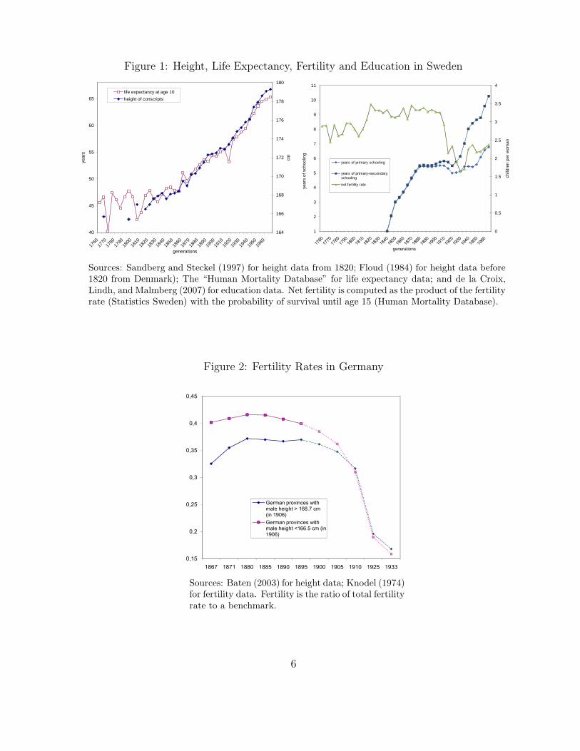
Figure 1: Height, Life Expectancy, Fertility and Education in Sweden
40
45
50
55
60
65
1760
1770
1780
1790
1800
1810
1820
1830
1840
1850
1860
1870
1880
1890
1900
1910
1920
1930
1940
1950
1960
generations
year
s
164
166
168
170
172
174
176
178
180
cm
life expectancy at age 10
height of conscripts
0
0.5
1
1.5
2
2.5
3
3.5
4
1
2
3
4
5
6
7
8
9
10
11
child
ren
per
wom
an
year
s of
sch
oolin
g
generations
years of primary schooling
years of primary+secondary schooling
net fertility rate
Sources: Sandberg and Steckel (1997) for height data from 1820; Floud (1984) for height data before1820 from Denmark); The “Human Mortality Database” for life expectancy data; and de la Croix,Lindh, and Malmberg (2007) for education data. Net fertility is computed as the product of the fertilityrate (Statistics Sweden) with the probability of survival until age 15 (Human Mortality Database).
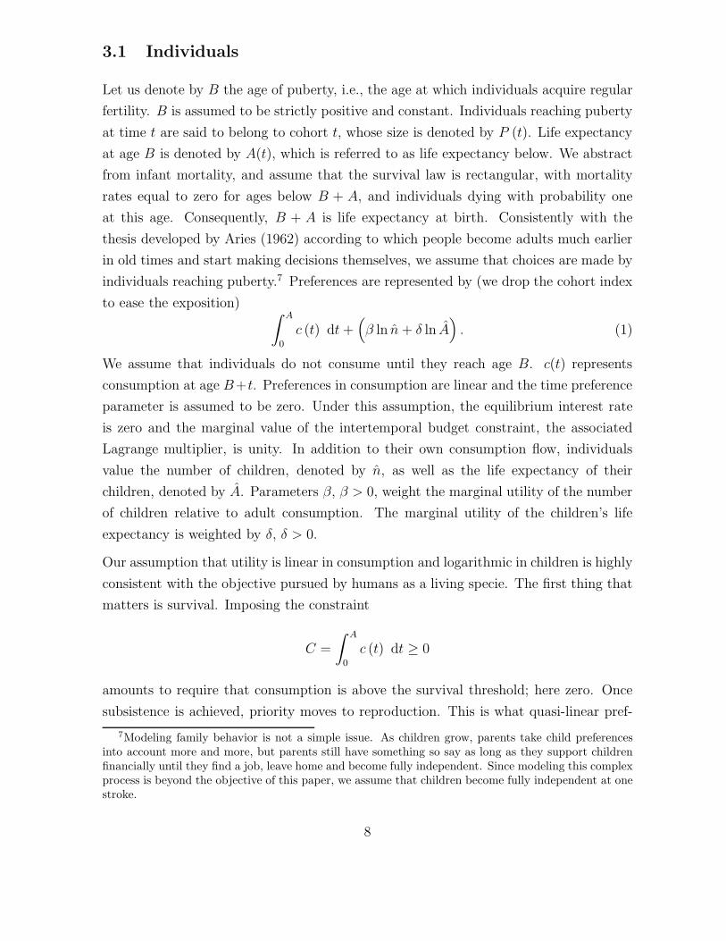
Figure 2: Fertility Rates in Germany
0,45
0,15
0,2
0,25
0,3
0,35
0,4
1867 1871 1880 1885 1890 1895 1900 1905 1910 1925 1933
German provinces with male height > 168.7 cm (in 1906)
German provinces with male height <166.5 cm (in 1906)
Sources: Baten (2003) for height data; Knodel (1974)for fertility data. Fertility is the ratio of total fertilityrate to a benchmark.
6
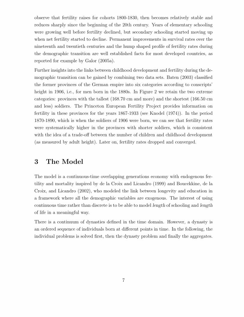
observe that fertility raises for cohorts 1800-1830, then becomes relatively stable and
reduces sharply since the beginning of the 20th century. Years of elementary schooling
were growing well before fertility declined, but secondary schooling started moving up
when net fertility started to decline. Permanent improvements in survival rates over the
nineteenth and twentieth centuries and the hump shaped profile of fertility rates during
the demographic transition are well established facts for most developed countries, as
reported for example by Galor (2005a).
Further insights into the links between childhood development and fertility during the de-
mographic transition can be gained by combining two data sets. Baten (2003) classified
the former provinces of the German empire into six categories according to conscripts’
height in 1906, i.e., for men born in the 1880s. In Figure 2 we retain the two extreme
categories: provinces with the tallest (168.70 cm and more) and the shortest (166.50 cm
and less) soldiers. The Princeton European Fertility Project provides information on
fertility in these provinces for the years 1867-1933 (see Knodel (1974)). In the period
1870-1890, which is when the soldiers of 1906 were born, we can see that fertility rates
were systematically higher in the provinces with shorter soldiers, which is consistent
with the idea of a trade-off between the number of children and childhood development
(as measured by adult height). Later on, fertility rates dropped and converged.
3 The Model
The model is a continuous-time overlapping generations economy with endogenous fer-
tility and mortality inspired by de la Croix and Licandro (1999) and Boucekkine, de la
Croix, and Licandro (2002), who modeled the link between longevity and education in
a framework where all the demographic variables are exogenous. The interest of using
continuous time rather than discrete is to be able to model length of schooling and length
of life in a meaningful way.
There is a continuum of dynasties defined in the time domain. However, a dynasty is
an ordered sequence of individuals born at different points in time. In the following, the
individual problems is solved first, then the dynasty problem and finally the aggregates.
7
3.1 Individuals
Let us denote by B the age of puberty, i.e., the age at which individuals acquire regular
fertility. B is assumed to be strictly positive and constant. Individuals reaching puberty
at time t are said to belong to cohort t, whose size is denoted by P (t). Life expectancy
at age B is denoted by A(t), which is referred to as life expectancy below. We abstract
from infant mortality, and assume that the survival law is rectangular, with mortality
rates equal to zero for ages below B + A, and individuals dying with probability one
at this age. Consequently, B + A is life expectancy at birth. Consistently with the
thesis developed by Aries (1962) according to which people become adults much earlier
in old times and start making decisions themselves, we assume that choices are made by
individuals reaching puberty.7 Preferences are represented by (we drop the cohort index
to ease the exposition)∫ A
0
c (t) dt +(
β ln n + δ ln A)
. (1)
We assume that individuals do not consume until they reach age B. c(t) represents
consumption at age B+t. Preferences in consumption are linear and the time preference
parameter is assumed to be zero. Under this assumption, the equilibrium interest rate
is zero and the marginal value of the intertemporal budget constraint, the associated
Lagrange multiplier, is unity. In addition to their own consumption flow, individuals
value the number of children, denoted by n, as well as the life expectancy of their
children, denoted by A. Parameters β, β > 0, weight the marginal utility of the number
of children relative to adult consumption. The marginal utility of the children’s life
expectancy is weighted by δ, δ > 0.
Our assumption that utility is linear in consumption and logarithmic in children is highly
consistent with the objective pursued by humans as a living specie. The first thing that
matters is survival. Imposing the constraint
C =
∫ A
0
c (t) dt ≥ 0
amounts to require that consumption is above the survival threshold; here zero. Once
subsistence is achieved, priority moves to reproduction. This is what quasi-linear pref-
7Modeling family behavior is not a simple issue. As children grow, parents take child preferencesinto account more and more, but parents still have something so say as long as they support childrenfinancially until they find a job, leave home and become fully independent. Since modeling this complexprocess is beyond the objective of this paper, we assume that children become fully independent at onestroke.
8
erences deliver. Reproduction covers the two relevant dimensions in the transmission of
genes: the quantity and survival of descendants.8
The technology producing human capital depends on the time allocated to education,
denoted by T :
h = µ (θ + T )α .
The productivity parameter µ and the parameter θ, which relates to schooling before
puberty, are strictly positive, and α ∈ (0, 1). θ ensures that human capital, and hence
income, are positive even if individuals choose not to go to school after age B.
The budget constraint takes the form
∫ A
0
c (t) dt + n Ψ(A) = µ (θ + T )α (A − T − φn) . (2)
The right hand side is the total flow of labor income under the assumption that one unit
of human capital produces one unit of good. For simplicity, we assume that people have
and raise their children immediately after finishing their studies and before becoming
active in the labor market. This greatly simplifies the dynastic structure of the model.
Raising a child takes a time interval of length φ > 0, implying that individuals work for
a period of length A − T − φn. Parental expenditure on each child’s development is
Ψ(A) = κ1
2
1
AA2, (3)
which implies that the expenditure is quadratic in A and inversely related to A.9 This
formulation is consistent with the complex interaction between nurture and nature ob-
served by biologists and psychologists. It stresses the difficulty of raising life expectancy
above that of the parents, reflecting how the genes interact with human behavior (the
environment) in building up a child body. The parameter κ > 0 measures the costs of
developing children in a broad sense.
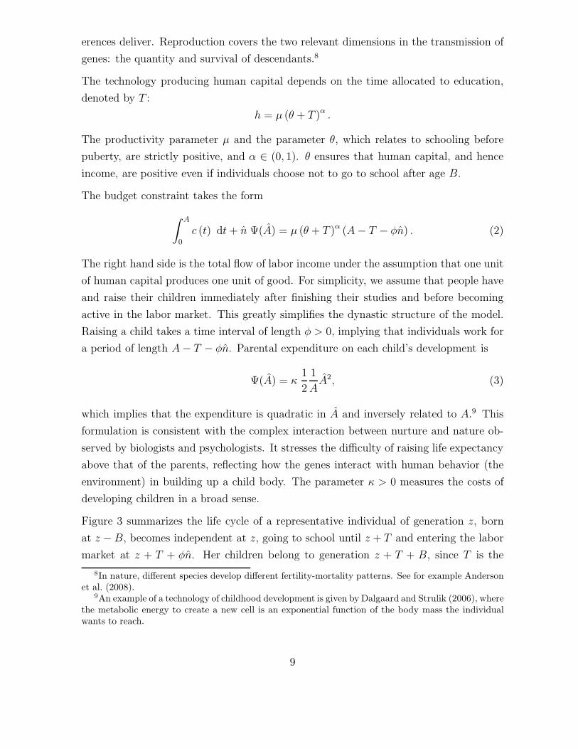
Figure 3 summarizes the life cycle of a representative individual of generation z, born
at z − B, becomes independent at z, going to school until z + T and entering the labor
market at z + T + φn. Her children belong to generation z + T + B, since T is the
8In nature, different species develop different fertility-mortality patterns. See for example Andersonet al. (2008).
9An example of a technology of childhood development is given by Dalgaard and Strulik (2006), wherethe metabolic energy to create a new cell is an exponential function of the body mass the individualwants to reach.
9
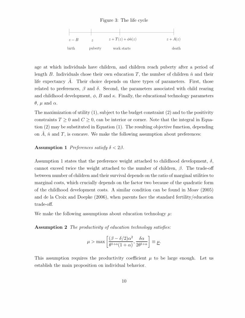
Figure 3: The life cycle
birth puberty work starts death
z − B z + T (z) + φn(z) z + A(z)z
age at which individuals have children, and children reach puberty after a period of
length B. Individuals chose their own education T , the number of children n and their
life expectancy A. Their choice depends on three types of parameters. First, those
related to preferences, β and δ. Second, the parameters associated with child rearing
and childhood development, φ, B and κ. Finally, the educational technology parameters
θ, µ and α.
The maximization of utility (1), subject to the budget constraint (2) and to the positivity
constraints T ≥ 0 and C ≥ 0, can be interior or corner. Note that the integral in Equa-
tion (2) may be substituted in Equation (1). The resulting objective function, depending
on A, n and T , is concave. We make the following assumption about preferences:
Assumption 1 Preferences satisfy δ < 2β.
Assumption 1 states that the preference weight attached to childhood development, δ,
cannot exceed twice the weight attached to the number of children, β. The trade-off
between number of children and their survival depends on the ratio of marginal utilities to
marginal costs, which crucially depends on the factor two because of the quadratic form
of the childhood development costs. A similar condition can be found in Moav (2005)
and de la Croix and Doepke (2006), when parents face the standard fertility/education
trade-off.
We make the following assumptions about education technology µ:
Assumption 2 The productivity of education technology satisfies:
µ > max
[(β − δ/2)α2
θ1+α(1 + α),
δα
2θ1+α
]
≡ µ.
This assumption requires the productivity coefficient µ to be large enough. Let us
establish the main proposition on individual behavior.
10
Proposition 1 Under Assumptions 1 and 2, there exist two thresholds A and A, 0 <
A < A, such that:
If A ≥ A, there is a unique interior solution satisfying
A2 =δ
κnA, (4)
T =α
1 + α(A − φn) −
θ
1 + α, (5)
n =β − δ/2
µφ(θ + T )−α . (6)
If A ≤ A < A, there is a unique corner solution with positive consumption satisfying
A2 =δ
κnA, (7)
T = 0, (8)
n =β − δ/2
µφθα. (9)
If 0 < A < A, there is a unique corner solution with zero consumption satisfying
A2 =δ
κ
µθαφ
β − δ/2A, (10)
T = 0, (11)
n =β − δ/2
βφA. (12)
Proof. Using the Kuhn-Tucker conditions for constrained optimization, we can identify
the two thresholds A and A and characterize the different regimes. See Appendix A.
Restriction A ≥ A in Proposition 1 states that parental life expectancy has to be large
enough for schooling to be positive. At the interior solution, Equation (4) shows the
trade-off faced by parents between the number and the life expectancy of their chil-
dren. The relation is negative, since the total cost of providing children with a good
body development increases as their number increases. Equation (5) is the standard
Ben-Porath (1967) result, as described by de la Croix and Licandro (1999), where life
expectancy positively affects the time allocated to education since it allows people to
work for a longer time. The term φn in Equation (5) shows an additional trade-off of
having children: parents expecting to have many children will postpone their entry into
11
the labor market, reducing the incentives to take additional education. This trade-off
also shows up in Equation (6).
When A ≤ A < A, parental life expectancy A is not long enough to render optimal a
positive investment in education. For lower levels of life expectancy, i.e. when A < A,
both education and consumption are zero.10 Expected life time earnings are so low that
parents use all their resources in bearing a limited number of children.
From now on, the interior solution, (4)-(6), and the corner solutions, (7)-(9) and (10)-
(12), are referred to as A = fA(A), T = fT (A) and n = fn(A). The effect of an increase
in A is given by Corollary 1:
Corollary 1 f ′
A(A) > 0;
f ′
n(A) < 0, for A ≥ A, f ′
n(A) = 0, for A ≤ A < A, and f ′
n(A) > 0 otherwise
f ′
T (A) > 0, for A ≥ A, and f ′
T (A) = 0 otherwise
Proof. See Appendix A.
In the interior solution, increased life expectancy raises optimal schooling and human
capital levels via the Ben-Porath effect. This increases the opportunity cost (time cost)
of raising children. Hence, the optimal number of children drops as life expectancy
increases.
In the corner solutions, since T = 0, a change in parental life expectancy does not affect
education, canceling the Ben-Porath effect. In the corner regime (7)-(9) the number
of children remains constant whatever the life expectancy, but childhood development
is still positively affected by life expectancy, since the efficiency of body development
activities depends positively on parental life expectancy. In the corner regime (10)-(12),
when consumption C is zero, however, the effect of life expectancy on the number and
survival of children reverses, since the number of children is directly determined by the
C = 0 constraint, which allows for more children as life expectancy, and hence life-cycle
income, increases. This is a pure income effect as in the Malthusian “positive check”
hypothesis.
10Imposing a strictly positive minimum consumption level with C ≥ C for the sake of realism wouldnot change the results. The only difference is that A would be larger and increasing in C.
12
3.2 Dynasties
Since individual decisions do not depend on aggregate variables, we can study the dy-
namics of life expectancy, fertility and education within dynasties separately, before the
analysis of the aggregates.
Let us consider the dynamics of life expectancy first. At any point t, individuals reaching
puberty belong to a representative dynasty with life expectancy A (t). Let us denote as
A1 the life expectancy of the first generation of this dynasty. The operator fA defined
above consists in a difference equation governing the evolution of the dynasty’s life
expectancy since
Ai+1 = Ai = fA(Ai),
where the index i = 1, 2, 3, ..., is associated with generations. From Proposition 1, for
any initial value A1 there exists a sequence of solutions Ti = f iT (A1), Ai = f i
A (A1) and
ni = f in (A1) for i = 1, 2, 3, ..., where X i is the ith consecutive application of operator X.
In the following, we characterize the dynamics of life expectancy. Once this has been
done, the sequence {A1, A2, ...} determines through the operators fT and fn the date
and size of the following generations.
Proposition 2 Under Assumptions 1 and 2, a stationary solution A = fA(A) exists, is
unique and globally stable.
Proof. See Appendix A.
Proposition 2 states that life expectancy converges to a constant value in the long run.
Consequently, from Proposition 1, fertility and education also converge to a constant
value. Demographic variables are then stationary, meaning that the demographic tran-
sition only occurs, as the name itself indicates, as a transitional phenomenon.
The results obtained so far allow us to assess some theoretical characteristics of the
demographic transition in our model. Consider Figure 4. The lower panel plots the
function fA(A). It describes a situation where the globally stable steady state is in the
modern regime. The top panel shows fertility as a function of life expectancy. Suppose
now that initial life expectancy is very low, below A. The dynamics of life expectancy
will be monotonic and converge to the steady state. A rise in life expectancy will firstly
drive fertility up (as long as the economy is in the Malthusian regime A < A), then
fertility will peak in the zone where A ≤ A < A (i.e. where T = 0 but C > 0), and
then decrease in the modern era. (Secondary) schooling will be zero until we reach the
13
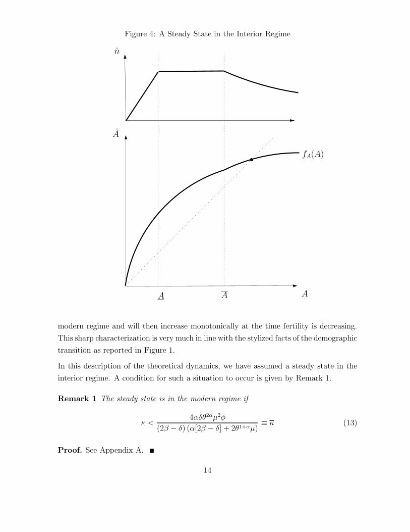
Figure 4: A Steady State in the Interior Regime
A
A
A A
fA(A)
n
modern regime and will then increase monotonically at the time fertility is decreasing.
This sharp characterization is very much in line with the stylized facts of the demographic
transition as reported in Figure 1.
In this description of the theoretical dynamics, we have assumed a steady state in the
interior regime. A condition for such a situation to occur is given by Remark 1.
Remark 1 The steady state is in the modern regime if
κ <4αδθ2αµ2φ
(2β − δ) (α[2β − δ] + 2θ1+αµ)≡ κ (13)
Proof. See Appendix A.
14
Condition (13) states that if the childhood development technology is cheap enough,
there is an interior steady state with positive education. Changing the value of κ is a
natural way of generating a demographic transition: if κ is initially high, the economy
may be in one of the corner regimes. Once κ decreases, body development becomes
more affordable, and the new steady state may move to the modern regime, with life
expectancy converging monotonically.
4 Simulating the Demographic Transition
In this section, we investigate to what extent changes in the cost of childhood develop-
ment helps reproducing the key facts of the demographic transition. The transition is
studied as the reaction to a change in the environment occurring slowly from 1700 and
leading the economy to a new balanced growth path in the 21st century characterized by
longer lives. For this purpose, we implement a change in cost of childhood development
as measured by parameter κ and analyze how the economy adjusts to this change.11
4.1 The Change in Parameter κ
Before analyzing the demographic transition as a response to a reduction in the cost of
childhood development, we need to discuss briefly the interpretation to be given to such
a change. The quantitative exercise requires, as explained in the following section, a slow
and long reduction in κ starting in the 18th century and lasting to our days, with more
than 80% of this reduction occurring between 1840 and 1960. Reducing the cost of body
development may be due to improvements in hygienic habits, medical treatments and
nutrition. Nobody would object to such progresses in the late nineteenth and twentieth
century. The references below claim that improvements in these dimensions started in
fact before the 19th century.
Johansson (1999) argues against the therapeutic nihilism denying that medicine had any
effectiveness before the end of the nineteenth century. Firstly, in the period 1500-1800,
medicine showed an increasingly experimental attitude: no improvement was effected
on the grounds of the disease theory (which was still mainly based on traditional ideas),
11A more sophisticated version of the model, in line with Galor and Weil (2000), would allow thedemographic transition to be associated with an endogenously generated industrial revolution. Thiscould be achieved by letting the body development technology, as measure by the inverse of κ, dependupon population size or density, for example.
15

but significant advances were made based on practice and empirical observations. For
example, although the theoretical understanding of how drugs work only came progres-
sively in the nineteenth century with the development of chemistry (Weatherall 1996),
the effectiveness of the treatment of some important diseases was improved thanks to
the practical use of new drugs coming from the New World. Second, the number of
books containing lifestyle advice increased significantly over the period 1750-1800, which
provides some indirect evidence on the fact that personal and domestic cleanness, for
example, became popular before the 19the century. Third, as early as 1829, Dr.F.B.
Hawkins wrote a book entitled Elements of Medical Statistics, in which he described
what could be called an early modern epidemiological transition. He describes a set of
diseases which were leading causes of death but could at the time be treated effectively:
leprosy, plague, sweating sickness, ague, typhus, smallpox, syphilis and scurvy. The cu-
mulative effects of these improvements could have produced a net increase in the efficacy
of medicine as early as in the eighteenth century (see de la Croix and Sommacal (2008)
for further arguments).
However, medicine did not play a major role during the 19th century, as claimed by
Omran (1971). “The reduction of mortality in Europe and most western countries during
the nineteenth century ... was determined primarily by ecobiologic and socioeconomic
factors. The influence of medical factors was largely inadvertent until the twentieth
century, by which time pandemics of infection had already receded significantly.” In the
same direction, refereing to the first half of the 19th century, Landes (1999) argues that
“Much of the increased life expectancy of these years has come from gains in prevention,
cleaner living rather than better medicine.” He relates it to reductions in the price of
washable cotton, along with the mass production of soap. In a recent survey conducted
by the British Medical Journal, medical professionals consider the sanitary revolution
of the nineteen century as the major medical milestones since 1840, leading medical
innovations as antibiotics, anaesthesia and vaccines.
The fundamental role of nutrition improvements on the reduction of mortality during
and before the Industrial Revolution has been stressed by McKeown and Record (1962),
and recently restated by Harris (2004).
16
4.2 The Demographic Transition
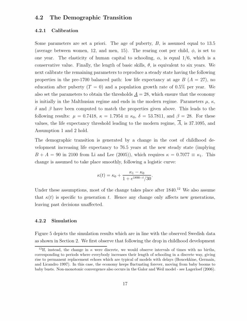
4.2.1 Calibration
Some parameters are set a priori. The age of puberty, B, is assumed equal to 13.5
(average between women, 12, and men, 15). The rearing cost per child, φ, is set to
one year. The elasticity of human capital to schooling, α, is equal 1/6, which is a
conservative value. Finally, the length of basic skills, θ, is equivalent to six years. We
next calibrate the remaining parameters to reproduce a steady state having the following
properties in the pre-1700 balanced path: low life expectancy at age B (A = 27), no
education after puberty (T = 0) and a population growth rate of 0.5% per year. We
also set the parameters to obtain the thresholds A = 28, which ensure that the economy
is initially in the Malthusian regime and ends in the modern regime. Parameters µ, κ,
δ and β have been computed to match the properties given above. This leads to the
following results: µ = 0.7418, κ = 1.7954 ≡ κ0, δ = 53.7811, and β = 28. For these
values, the life expectancy threshold leading to the modern regime, A, is 37.1095, and
Assumption 1 and 2 hold.
The demographic transition is generated by a change in the cost of childhood de-
velopment increasing life expectancy to 76.5 years at the new steady state (implying
B + A = 90 in 2100 from Li and Lee (2005)), which requires κ = 0.7077 ≡ κ1. This
change is assumed to take place smoothly, following a logistic curve:
κ(t) = κ0 +κ1 − κ0
1 + e1890−t/30.
Under these assumptions, most of the change takes place after 1840.12 We also assume
that κ(t) is specific to generation t. Hence any change only affects new generations,
leaving past decisions unaffected.
4.2.2 Simulation
Figure 5 depicts the simulation results which are in line with the observed Swedish data
as shown in Section 2. We first observe that following the drop in childhood development
12If, instead, the change in κ were discrete, we would observe intervals of times with no births,corresponding to periods where everybody increases their length of schooling in a discrete way, givingrise to permanent replacement echoes which are typical of models with delays (Boucekkine, Germain,and Licandro 1997). In this case, the economy keeps fluctuating forever, moving from baby booms tobaby busts. Non-monotonic convergence also occurs in the Galor and Weil model - see Lagerloef (2006).
17
Figure 5: Example of dynamics - drop in κ
1700 1750 1800 1850 1900 1950
20
30
40
50
60
70
Cohorts' life expectancy at puberty
1700 1750 1800 1850 1900 1950
1.02
1.04
1.06
1.08
1.10
1.12
1.14
Total cohort fertility rate
1750 1800 1850 1900 1950
0.5
1.0
1.5
2.0
2.5
3.0
3.5
Cohorts' education
costs cohorts’ life expectancy increases monotonically over time. Note that Figure 5
stops well before life expectancy has converged to steady state. Cohorts’ secondary
education remains nil up to the beginning of the 20th century when the economy enters
the modern regime, and it increases from then monotonically. Notice that the magnitude
of the increase is about right, with secondary schooling reaching 3 years around 1970.
Cohorts’ fertility (per individual, to be multiplied by 2 to get fertility per women)
first increases as long as the economy is in the Malthusian regime, then peaks in the
intermediary regime, to monotonically drop as a consequence of the trade-off between
education and the number of children in the modern era.
4.3 Regional Variations
We conclude from the above simulation exercise that our model is able to reproduce
the main features of the demographic transition. Another question is whether we can
also shed some light on regional variations in the demographic transition. Considering
the German data presented in Figure 2, we have seen that adult height (a proxy for
18

childhood development) and fertility were negatively associated across provinces on the
eve of the twentieth century.
At that time, the prevailing regime is the one where consumption is above subsistence
but it is not yet optimal to invest in (secondary) education. One reason for different
places exhibiting different fertility and height levels during this phase of demographic
transition is that the productivity parameter µ could vary in different places. The high
µ regions will have lower fertility and taller citizens as it is clear from Equations (7)
and (9). A similar argument can be made by letting the other parameters vary across
regions. For example, regions with a higher θ or φ will also have tall parents with few
children.
In Figure 2 we also observe that differences across regions seem to vanish as soon as the
interior regime is reached in the beginning of the twentieth century. This convergence
could reflect a reduction in the variance of the distribution of µ across regions, which
would be the case for example if the education system is more and more framed by a
central authority.
5 From Malthus to Modern Growth
The transition from a world of low economic growth with high mortality and high fertility
to one with low mortality and fertility but sustained growth has been the subject of
intensive research in recent years.13 In this literature, the relation between growth
and fertility results from the quantity/quality trade-off faced by parents between the
number of children and their education. Indeed, the gradual increase in the observed
level of human capital during the nineteenth century ‘has led researchers to argue that
the increasing role of human capital in the production process induced households to
increase investment in the human capital of their offspring, ultimately leading to the
onset of the demographic transition’ (Galor 2005b).
If the rise in education was indeed driven by a stronger demand for skills from the indus-
trial sector, one should have observed a rise in the skill premium during and following
the industrial revolution. Looking for such evidence, Clark (2005) computes a skill pre-
mium over the period 1220-1990 in two different ways. First by measuring the relative
13Rostow (1960) presents an early attempt to understand the transition from stagnation to growth.The first modern treatment of the issue is in the seminal paper by Galor and Weil (2000). See Doepke(2006) for a recent survey.
19

wage of all skilled building workers 14 relative to all laborers and, second, by using only
those observations in which there is a matched pair for the same place and year of wages
for craftsmen and laborers. The two methods lead to the same conclusion: the skill
premium did not rise during the Industrial Revolution. And Clark concludes that ‘The
market premium for skills, does not explain the increased investment in human skills
evident after 1600.’ Hence, we might wonder whether the human capital interpretations
of the Industrial Revolution are based on the right trade-off. The new mechanism we
develop in this paper could be seen as an alternative to the usual one.
5.1 A Growth Model
We introduce endogenous growth to the model in Section 3 by adding a human capital
externality in the education technology:
h = µ (θ + T )α H,
where H is human capital per worker. It may reflect, for example, the quality of educa-
tion or the cultural ambience in the society.
To keep utility balanced in a growing economy, we assume that preferences are
∫ A
0
c (z) dz + H(
β ln n + δ ln A)
, (14)
where H now multiplies the term associated with children, implying that the value of
children also grows with cultural ambience in the society. Finally, for similar reasons,
childhood development costs are also indexed on average human capital per worker:
Ψ(A) = κ1
2
H
AA2. (15)
These assumptions do not affect the household decision problem and all the results in
the previous sections can be applied directly.
20
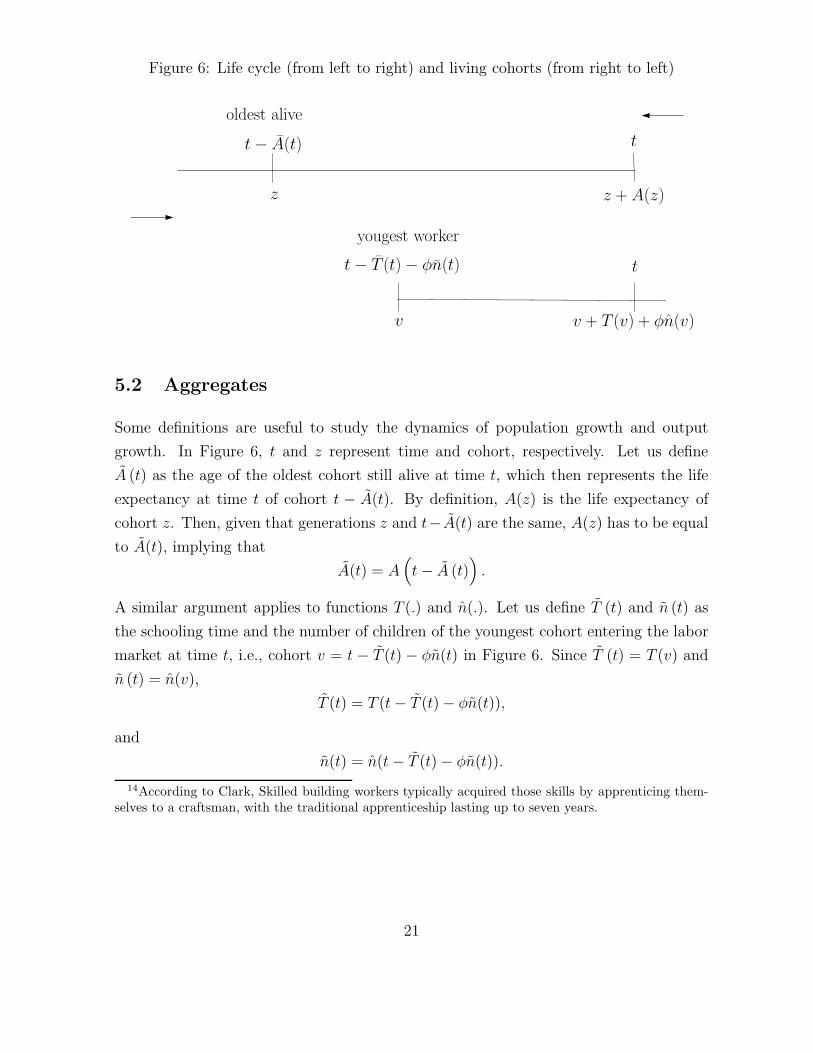
Figure 6: Life cycle (from left to right) and living cohorts (from right to left)
v + T (v) + φn(v)
z + A(z)
tt − A(t)
oldest alive
t − T (t) − φn(t)
z
v
t
yougest worker
5.2 Aggregates
Some definitions are useful to study the dynamics of population growth and output
growth. In Figure 6, t and z represent time and cohort, respectively. Let us define
A (t) as the age of the oldest cohort still alive at time t, which then represents the life
expectancy at time t of cohort t − A(t). By definition, A(z) is the life expectancy of
cohort z. Then, given that generations z and t− A(t) are the same, A(z) has to be equal
to A(t), implying that
A(t) = A(
t − A (t))
.
A similar argument applies to functions T (.) and n(.). Let us define T (t) and n (t) as
the schooling time and the number of children of the youngest cohort entering the labor
market at time t, i.e., cohort v = t − T (t) − φn(t) in Figure 6. Since T (t) = T (v) and
n (t) = n(v),
T (t) = T (t − T (t) − φn(t)),
and
n(t) = n(t − T (t) − φn(t)).
14According to Clark, Skilled building workers typically acquired those skills by apprenticing them-selves to a craftsman, with the traditional apprenticeship lasting up to seven years.
21

Total population is computed by integrating over all the living cohorts:
N (t) =
∫ t+B
t−A(t)
P (z) dz, (16)
from the oldest t − A(t) to the youngest t + B. The cohort size P (z) is given by
P (z + T (z) + B) = n (z) P (z) , (17)
since members of cohort z have n(z) children at time z + T (z), who belong to cohort
z + T (z) + B.
Aggregate human capital is defined by the human capital of active cohorts
H (t) =
∫ t−T (t)−φn(t)
t−A(t)
P (z) µ (θ + T (z))α H (z)︸ ︷︷ ︸
h(z)
dz (18)
where average human capital per worker is given by
H (t) =H (t)
E (t),
and total employment E (t) is
E (t) =
∫ t−T (t)−φn(t)
t−A(t)
P (z) dz.
The technology producing the consumption good, the only final good in this economy,
is linear in aggregate human capital with productivity one, implying that the real wage
per unit of human capital is unity. Output per capita is then H(t)/N(t).
5.3 Balanced Growth Path
A balanced growth path is an equilibrium path where population grows at rate η, human
capital at rate γ, and, the demographic variable T , n and A are all constant. From
Equation (17), the grow rate of cohorts’ size is such that eη(T+B) = n, i.e.
η =ln (n)
T + B,
22
with P (t) = P ⋆eηt, P ⋆ > 0. The population growth rate depends on the fertility rate n
and on the age at child’s birth B + T . At a given fertility rate, the smaller the age at
birth, the larger the frequency of births and thus the population growth rate.
Total population, as defined in Equation (16), evolves along a balanced growth path
following
N(t) = N⋆ eηt = P ⋆ eηB − e−ηA
ηeηt,
with N⋆ > 0. Population also grows at rate η and its size depends positively, as expected,
on life expectancy. When η approaches zero, i.e., when population is constant, its size is
given by N(t) = P ⋆(B + A), which is the product of the cohort size and life expectancy
at birth. Along a balanced growth path, the active population is given by
E (t) = E⋆ eηt = P ⋆ e−η(T+φn) − e−ηA
ηeηt.
Similarly as for total population, when η approaches zero E(t) converges to P ⋆(A−T −
φn), where the term in brackets is the length of active life.
Finally, the growth rate of human capital γ satisfies at the balanced growth path
γ =P ⋆
E⋆µ(θ + T )α
(e−γ(T+φn) − e−γA
).
To understand this result better, let us differentiate, at the balanced growth path, the
definition of H(t) in Equation (18) with respect to time:
H ′(t) = P (t − T − φn)h(t − T − φn) − P (t − A)h(t − A).
The change in aggregate human capital is the difference between the human capital of
the youngest workers and that of the oldest. From the human capital technology, and
using the balanced growth path assumption
γ =H ′(t)
H(t)=
P ⋆
E⋆µ(θ + T )α
(e−γ(T+φn) − e−γA
).
The first term on the r.h.s, P ⋆/E⋆, derives directly from the assumption that per worker
human capital affects the human capital of the current cohort. If, instead of normalizing
total human capital by E, we normalized it by P , this term would vanish. It basically
corresponds to the length of active life. The second term reflects the fact that both
23
Figure 7: Example of dynamics - drop in κ - human capital
1750 1800 1850 1900 1950
-3.65
-3.60
-3.55
-3.50
-3.45
log GDP per capita
1750 1800 1850 1900 1950
0.002
0.004
0.006
0.008
0.010
Population growth rate
the oldest and the youngest cohort share the same human capital technology, with a
common length of education. For this reason, the term µ(θ + T )α is common. Finally,
the last term in brackets reflects the fact that aggregate human capital was not the same
at the time the two cohorts were at school, the difference depending on the growth rate
itself and the age difference between the cohorts.
5.4 Simulating the Transition to Modern Growth
No theorem is available to assess the asymptotic behavior of the solutions of our dynamic
system directly, and in particular, whether income per capita converges to its balanced
growth path.15 In the simulation below though, the solution converges asymptotically
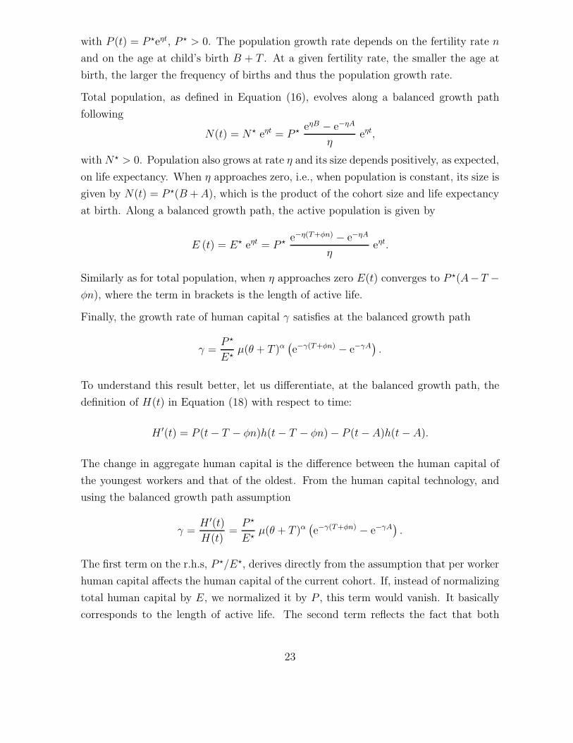
to the balanced growth path.16
Figure 7 illustrates the complex relationship between the demographic transition and the
transition from Malthus to Modern growth. As long as the economy is in the Malthusian
regime, an increase in life expectancy induces an increase of the population growth rate.
Since fertility goes up, the associated raise in the dependency ratio reduces income per
capita. In the intermediary regime, with consumption above subsistence but still no
education, increases in life expectancy promote growth, because it raises adult longevity
and the number of workers per dependent children. Finally, in the modern era, the take-
off of education generates an acceleration in growth and a switch to a balanced growth
15No direct stability theorem is available for delay differential systems with more than one delaysince the stability outcomes depend on the particular values of the delays. See Mahaffy, Joiner, andZak (1995).
16The simulation was performed using the method in Boucekkine, Licandro, and Paul (1997).
24
path with positive income growth.17 Notice that the model does not generate enough
growth compared to observations, as it relies only on population and human capital as
the engine of growth.
6 Conclusion
The epidemiology literature stresses that life expectancy depends greatly on body de-
velopment during childhood. Both better nutrition and lower exposure to infections
leads to increased body height and a longer life. We have proposed a theory of the
demographic transition based on this fact. The novel mechanism of the model is that
parents face a trade-off between the quantity of children they have and the amount they
can afford to spend on childhood development of each of them. Parents like to have
many children, but they also care about their longevity. Having many children pre-
vents parents spending much on their body development. If its cost decreases, parents
will increase their investment in their children’s longevity. The number of children will
first increase in the Malthusian regime as a consequence of higher lifetime income. As
longevity rises, fertility starts falling as a result of the trade-off faced by parents between
investing in their own human capital and spending time rearing children. Following the
trade-off between the number of children and childhood development, adult longevity
keeps increasing.
The model we have developed reproduces the characteristics of the demographic tran-
sition well, displaying the appealing features that longer education delays birth and
reduces fertility. Our theory can be seen as an alternative to the one based on a rise in
the return to human capital investment induced by economic progress, leading parents
to substitute quality for quantity. A distinctive implication of our theory is that im-
provements in childhood development should precede the increase in education. Taking
height as a proxy for childhood development, we have observed just such a pattern in
Swedish historical data.
Our theory can also provide an explanation for the puzzling fact that height at age
18 is a strong predictor of education attained later in life (Magnusson, Rasmussen,
and Gyllensten (2006) showed that Swedish men taller than 194 cm were two to three
times more likely to obtain a higher education than men shorter than 165 cm), even
17The slowdown around 1900 is related to the fact that the first educated generations postpone theirentry on the labor market.
25
after controlling for parental socioeconomic position, other shared family factors, and
cognitive ability. A further test of our theory would consist of checking whether family
size is related to childhood development as measured by average height on historical
micro-data.
References
Aisa, Rosa, and Fernando Pueyo. 2006. “Government health spending and growth in
a model of endogenous longevity.” Economics Letters 90 (2): 249–253 (February).
Anderson, Holly B., Melissa Emery Thompson, Cheryl D. Knott, and Lori Perkins.
2008. “Fertility and mortality patterns of captive Bornean and Sumatran
orangutans: is there a species difference in life history?” Journal of Human Evolu-
tion 54 (February): 34–42.
Aries, Philippe. 1962. Centuries of Childhood. New York: Alfred A. Knopf.
Barker, David, and Clive Osmond. 1986. “Infant mortality, childhood nutrition, and
ischaemic heart disease in England and Wales.” Lancet i:1077–1088.
Baten, Joerg. 2003. “Anthropometrics, consumption, and leisure: the standard of
living.” In Germany: A New Social and Economic History, Vol III: 1800-1989,
edited by Sheilagh Ogilvie and Richard Overy. London: Edward Arnold Press.
Baten, Jorg, and John Komlos. 1998. “Review: Height and the Standard of Living.”
The Journal of Economic History 58 (3): 866–870.
Ben-Porath, Yoram. 1967. “The production of human capital and the life-cycle of
earnings.” Journal of Political Economy 75 (4): 352–365.
Blackburn, Keith, and Giam Petro Cipriani. 2002. “A model of longevity, fertility and
growth.” Journal of Economic Dynamics and Control 26 (1): 187–204.
Boucekkine, Raouf, David de la Croix, and Omar Licandro. 2002. “Vintage human
capital, demographic trends and endogenous growth.” Journal of Economic Theory
104:340–375.
. 2003. “Early mortality declines at the dawn of modern growth.” Scandinavian
Journal of Economics 105:401–418.
Boucekkine, Raouf, Marc Germain, and Omar Licandro. 1997. “Replacement echoes in
the vintage capital growth model.” Journal of Economic Theory 74 (2): 333–348.
26

Boucekkine, Raouf, Omar Licandro, and Christopher Paul. 1997. “Differential-
difference equations in economics: On the numerical solution of vintage capital
growth models.” Journal of Economic Dynamics and Control 21:347–362.
Cervellati, Matteo, and Uwe Sunde. 2005. “Human capital formation, life expectancy
and the process of development.” American Economic Review 95 (5): 1653–1672.
. 2007. “Fertility, Education, and Mortality: A Unified Theory of the Economic
and Demographic Transition.” mimeo, IZA, Bonn.
Chakraborty, Shankha. 2004. “Endogenous lifetime and economic growth.” Journal of
Economic Theory 116 (1): 119–137.
Chakraborty, Shankha, and Mausumi Das. 2005. “Mortality, human capital and per-
sistent inequality.” Journal of Economic Growth 10 (2): 159–192.
Clark, Gregory. 2005. “The Condition of the Working Class in England, 1209-2004.”
Journal of Political Economy 113 (6): 1307–1340.
Crimmins, Eileen, and Caleb Finch. 2006. “Infection, inflammation, height, and
longevity.” Proceedings of the National Academy of Sciences of the United States
of America 103:498–503.
Dalgaard, Carl-Johan, and Holger Strulik. 2006, September. “Subsistence - A Bio-
economic Foundation of the Malthusian Equilibrium.” Discussion papers 06–17,
University of Copenhagen. Department of Economics (formerly Institute of Eco-
nomics).
de la Croix, David, and Matthias Doepke. 2006. “To Segregate or to Integrate: Edu-
cation Politics and Democracy.” Discussion paper 5799, C.E.P.R.
de la Croix, David, and Omar Licandro. 1999. “Life expectancy and endogenous
growth.” Economics Letters 65 (2): 255–263.
de la Croix, David, Thomas Lindh, and Bo Malmberg. 2007. “Economic Growth and
Education Since 1800: How Much does Longer Life Explain?” unpublished.
de la Croix, David, and Alessandro Sommacal. 2008. “A Theory of Medical Effec-
tiveness, Differential Mortality, Income Inequality and Growth for Pre-Industrial
England.” Mathematical Population Studies, p. forthcoming.
Doepke, Matthias. 2004. “Accounting for Fertility Decline During the Transition to
Growth.” Journal of Economic Growth 9 (3): 347–383.
27
. 2006. “Growth Takeoffs.” Working paper 847, UCLA Department of Eco-
nomics. forthcoming in the New Palgrave Dictionary of Economics, 2nd Edition.
Floud, Roderick. 1984, April. “The Heights of Europeans Since 1750: A New Source For
European Economic History.” Working paper 1318, National Bureau of Economic
Research, Inc.
Fogel, Robert. 1994. “Economic growth, population theory and physiology: the bearing
of long-term processes on the making of economic policy.” American Economic
Review 84 (3): 369–395.
Galor, Oded. 2005a. “The Demographic Transition and the Emergence of Sustained
Economic Growth.” Journal of the European Economic Association 3 (23): 494–
504.
. 2005b. “From Stagnation to Growth: Unified Growth Theory.” Chapter 4
of Handbook of Economic Growth, edited by Philippe Aghion and Steven Durlauf,
Volume 1 of Handbook of Economic Growth, 171–293. Elsevier.
Galor, Oded, and Omer Moav. 2005. “Natural Selection and the Evolution of Life
Expectancy.” Discussion papers 5373, C.E.P.R.
Galor, Oded, and David Weil. 2000. “Population, technology, and growth: from the
Malthusian regime to the demographic transition and beyond.” American Economic
Review 90 (4): 806–828.
Harris, Bernard. 2001. “‘The child is father of man.’ The relationship between child
health and adult mortality in the 19th and 20th centuries.” International Journal
of Epidemiology 30:688–696.
. 2004. “Public health, nutrition and the decline of mortality: The McKeown
thesis revised.” Social History of Medicine 17:379–407.
Hazan, Moshe, and Hosny Zoabi. 2006. “Does longevity cause growth? A theoretical
critique.” Journal of Economic Growth 11:363–376.
Johansson, Ryan. 1999. “Death and the doctors: medicine and elite mortality in
Britain from 1500 to 1800.” Cambridge Group for the History of Population and
Social Structure Working Paper Series. No. 7.
Kalemli-Ozcan, Sebnem. 2002. “Does the Mortality Decline Promote Economic
Growth?” Journal of Economic Growth 7:411–439.
28

Kermack, William, Anderson McKendrick, and P McKinlay. 1934. “Death Rates in
Great Britain and Sweden: some general regularities and their significance.” Lancet
i:698–703.
Knodel, John. 1974. The decline of fertility in Germany, 1871-1939. Princeton: Princ
eton University Press.
Lagerloef, Nils-Petter. 2003. “From Malthus to modern growth: can epidemics explain
the three regimes ?” International Economic Review 44 (2): 755–777.
. 2006. “The Galor-Weil Model Revisited: A Quantitative Exercise.” Review of
Economic Dynamics 9:116–142.
. 2007. “Violence.” mimeo, York University, Canada.
Landes, David. 1999. The Wealth and Poverty of Nations. New York: W.W. Norton
& Company.
Li, Nan, and Ronald Lee. 2005. “Coherent mortality forecasts for a group of popula-
tions: An extension of the Lee-Carter method.” Demography 42 (3): 575594.
Magnusson, Patrik, Finn Rasmussen, and Ulf Gyllensten. 2006. “Height at age 18
years is a strong predictor of attained education later in life: cohort study of over
950,000 Swedish men.” International Journal of Epidemiology 35 (3): 658–663.
Mahaffy, Joseph, Kathryn Joiner, and Paul Zak. 1995. “A Geometric Analysis of
Stability Regions for a Linear Differential Equation with two delays.” International
Journal of Bifurcation and Chaos 5 (3): 779–796.
McKeown, Thomas, and R. G. Record. 1962. “Reasons for the Decline of Mortality
in England and Wales during the Nineteenth Century.” Population Studies 16 (3):
94–122.
Moav, Omer. 2005. “Cheap Children and the Persistence of Poverty.” Economic
Journal 115 (500): 88–110.
Murphy, Kevin, and Robert Topel. 2006. “The Value of Health and Longevity.” Journal
of Political Economy 114:871–904.
Omran, Abdel. 1971. “The Epidemiologic Transition: A Theory of the Epidemiology
of Population Change.” Milbank Memorial Fund Quarterly 49:509–538.
Pinker, Steven. 2004. “Why nature & nurture won’t go away.” Daedalus 133 (4): 5–17.
Rostow, Walt. 1960. The Stages of Economic Growth. New York: Cambridge University
Press.
29
Sandberg, Lars, and Richard Steckel. 1997. “Was Industrialization Hazardous to your
Health? Not in Sweden.” In Health and Welfare during Industrialization, edited by
Richard Steckel and Roderick Floud. University of Chicago Press.
Sanso, Marcos, and Rosa M. Aisa. 2006. “Endogenous longevity, biological deterioration
and economic growth.” Journal of Health Economics 25 (3): 555–578.
Silventoinen, Karri. 2003. “Determinants of Variation in Adult Body Height.” Journal
of Biosocial Science 35:263–285.
Soares, Rodrigo. 2005. “Mortality Reductions, Educational Attainment, and Fertility
Choice.” American Economic Review 95(3):580–601.
Waaler, Hans. 1984. “Height, weight and mortality: the Norwegian experience.” Acta
medica Scandinavica. Supplementum 679:1–56.
Weatherall, Miles. 1996. “Drug treatment and the rise of pharmacology.” In Cambridge
Illustrated History: Medicine. Cambridge: Cambridge University Press.
Weil, David. 2007. “Accounting for the Effect of Health on Economic Growth.” Quar-
terly Journal of Economics 122:1265–1306.
Wordsworth, William. 1802. My heart leaps up when I behold. Poem.
30

A Proofs of Propositions
Proof of Proposition 1
After substituting the integral in (2) into (1), the objective becomes
(
β ln n + δ ln A)
+ µ (θ + T )α (A − T − φn) − n
(
κ
2
A2
A
)
︸ ︷︷ ︸
C
which is maximized under the restrictions T ≥ 0 and C ≥ 0.
First order conditions to this problem are (omitting the Kuhn-Tucker conditions):
(1 + η)A2 =δ
κnA (A.1)
(1 + η)αµ (θ + T )α−1 (A − T − φn) = (1 + η)µ (θ + T )α − λ (A.2)
1
n
(
β −δ
2
)
= (1 + η)µ (θ + T )α φ (A.3)
where λ and η are the Kuhn-Tucker multipliers associated with the constraints T ≥ 0
and C ≥ 0, respectively. The interior solution (4)-(6) is (A.1)-(A.3) under η = λ = 0.
The corner solution (7)-(9) results from the same system under η = T = 0, and finally,
the corner solution (10)-(12) results from the first order conditions under T = C = 0.
Under Assumption 2, η = C = 0 is not optimal.
Interior Regime. The solution to the first order conditions (4)-(6) exists and is unique
iff the loci in (5) and (6) cut once and only once for positive n and T , and C ≥ 0 at
the solution. The locus in (5) is a straight line with negative slope and cuts the n axes
at A−θ/αφ
≡ n0, see Figure A.1. The locus in (6) has a negative slope, is convex, and
is such that n goes to zero when T goes to infinity and cuts the n axes at β−δ/2µφθα ≡ n1.
Comparing these two points and imposing n0 ≥ n1 leads to the condition A ≥ A, where
A =β − δ
2
µθα+
θ
α.
Substituting (4) and (5) in the definition of C gives
C =µ
α(θ + T )1+α −
δ
2,
31
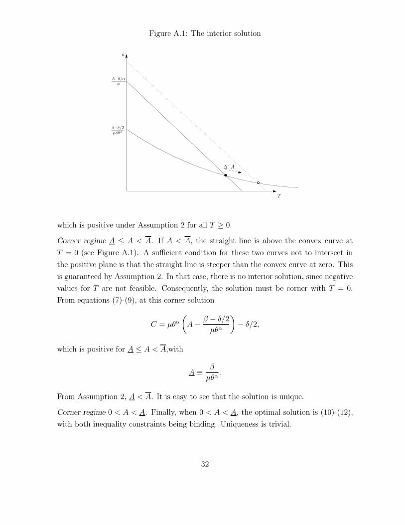
Figure A.1: The interior solution
β−δ/2µφθα
A−θ/α
φ
∆+A
n
T
which is positive under Assumption 2 for all T ≥ 0.
Corner regime A ≤ A < A. If A < A, the straight line is above the convex curve at
T = 0 (see Figure A.1). A sufficient condition for these two curves not to intersect in
the positive plane is that the straight line is steeper than the convex curve at zero. This
is guaranteed by Assumption 2. In that case, there is no interior solution, since negative
values for T are not feasible. Consequently, the solution must be corner with T = 0.
From equations (7)-(9), at this corner solution
C = µθα
(
A −β − δ/2
µθα
)
− δ/2,
which is positive for A ≤ A < A,with
A ≡β
µθα.
From Assumption 2, A < A. It is easy to see that the solution is unique.
Corner regime 0 < A < A. Finally, when 0 < A < A, the optimal solution is (10)-(12),
with both inequality constraints being binding. Uniqueness is trivial.
32

Proof of Corollary 1
For the interior solution, we apply the implicit function theorem to (4)-(6), which leads
to
f ′
A = dA/dA =
√
Aδ
nκ
(T (α + 1) + θ + α((A − nφ)α + θ))
2A((α + 1)(T + θ) − nα2φ).
The numerator is positive. Under Assumption 2, the denominator is also positive. The
results for f ′
n and f ′
T can be proved using the same arguments. For the corner solutions,
the result is straightforward.
Proof of Proposition 2
Let us denote the function fA(.) by fA1(.) when A ≥ A, fA2(.) when A ≤ A < A, and
fA3(.) when 0 < A < A. The dynamics of life expectancy following Ai+1 = fA(Ai) are
monotonic because fA is continuous and non-decreasing.
Let us first prove the existence of a solution. From corollary 1, f ′
A(A) > 0. It is easy
to see that limA→0 fA(A) = limA→0 fA3(A) > 0. To prove the existence it is enough to
show
limA→∞
fA(A)
A= lim
A→∞
fA1(A)
A= 0.
From (5) and (6)
n = cste(A − φn)−α.
Substituting in (4), and dividing by A2 gives
(
A
A
)2
= cste(A − φn)α
A.
Since limA→∞ fn(A) = 0, it’s now easy to see that limA→∞
fA1(A)A
= 0.
Let us now prove its unicity. For 0 < A < A, the function fA3(.) is increasing and
concave, with fA3(0) = 0 and f ′
A3(0) = ∞, implying that if it crosses the diagonal on
the interval (0, A), it crosses it only once.
Function fA2(.) is increasing and concave, with fA2(0) = 0 and f ′
A2(0) = ∞, implying
that if it crosses the diagonal on the interval [A, A), it crosses it only once.
33

Finally, let us prove that f ′
A1(A) < 1 for any fixed point of fA1(.) in A ≥ A. From the
implicit function theorem applied to (4)-(6),
dA
A/dA
A=
1
2
(1 + α)(A − φn)
A − (1 + α)n.
At a fixed point of fA1, since Corollary 1 shows that f ′
A(A) > 0 in this interval, the
denominator must be strictly positive. It is then easy to see that f ′
A(A) < 1 iff A >1+α1−α
φn. Since, from Corollary 1, f ′
n(.) < 0 in this interval, f ′
A(A) < 1 for all A ≥ A iff
A > 1+α1−α
φn, which holds under Assumption 2.
Global stability is then trivial, since fA is above the diagonal before the unique steady
state equilibrium and below it afterwards.
Proof of Remark 1
A steady state for A in the interior regime exists iff there is a solution to the system
(4)-(6) evaluated at the steady state. Eliminating A and n from Equation (5) using
Equations (4) and (6) we find that the steady state T should satisfy:
T (1 + α) + θ = α
(2δφµ(T + θ)α
κ(2β − δ)−
(2β − δ)(T + θ)−α
2µ
)
The left hand side is a linear increasing function of T . The right hand side is a concave
function of T , with a slope going to zero as T goes to infinity. A sufficient condition for
existence and uniqueness of a stationary solution is that the right hand side is larger
than the left hand side at T = 0. This leads to Condition (13).
34