The Climate and the Economy(Preliminary - do not quote or distribute without permission).

John Hassler, Per Krusell and Conny Olovsson This version: April 2019

March 19, 2020

Contents

1 Integrated Assessment Models —An introduction 3

2 The climate 42.1 The Greenhouse effect . . . . . . . . . . . . . . . . . . . . . . . . . . . . . . . . . . . 42.2 Forcing and the energy budget . . . . . . . . . . . . . . . . . . . . . . . . . . . . . . 52.3 Feedbacks . . . . . . . . . . . . . . . . . . . . . . . . . . . . . . . . . . . . . . . . . . 8

2.3.1 Feedbacks and uncertainty . . . . . . . . . . . . . . . . . . . . . . . . . . . . . 102.4 Total Forcing . . . . . . . . . . . . . . . . . . . . . . . . . . . . . . . . . . . . . . . . 122.5 Heating of the oceans . . . . . . . . . . . . . . . . . . . . . . . . . . . . . . . . . . . 122.6 Global Circulation Models . . . . . . . . . . . . . . . . . . . . . . . . . . . . . . . . . 142.7 Historical climate . . . . . . . . . . . . . . . . . . . . . . . . . . . . . . . . . . . . . . 172.8 More recent changes in the climate . . . . . . . . . . . . . . . . . . . . . . . . . . . . 192.9 Summary . . . . . . . . . . . . . . . . . . . . . . . . . . . . . . . . . . . . . . . . . . 20

3 Carbon circulation 213.1 The stock-flow approach . . . . . . . . . . . . . . . . . . . . . . . . . . . . . . . . . . 213.2 Human Influence on Carbon Circulation . . . . . . . . . . . . . . . . . . . . . . . . . 233.3 Size of fossil reserves . . . . . . . . . . . . . . . . . . . . . . . . . . . . . . . . . . . . 233.4 A Linear Carbon Circulation Model . . . . . . . . . . . . . . . . . . . . . . . . . . . 243.5 Carbon circulation in a DICE-type model . . . . . . . . . . . . . . . . . . . . . . . . 263.6 Depreciation models . . . . . . . . . . . . . . . . . . . . . . . . . . . . . . . . . . . . 273.7 A linear relation between emissions and temperature . . . . . . . . . . . . . . . . . . 283.8 References . . . . . . . . . . . . . . . . . . . . . . . . . . . . . . . . . . . . . . . . . . 30

4 Public economics 324.1 Consumer theory . . . . . . . . . . . . . . . . . . . . . . . . . . . . . . . . . . . . . . 324.2 The first theorem of welfare economics . . . . . . . . . . . . . . . . . . . . . . . . . . 334.3 Externalities . . . . . . . . . . . . . . . . . . . . . . . . . . . . . . . . . . . . . . . . 35

4.3.1 An example with a consumer externality . . . . . . . . . . . . . . . . . . . . . 354.3.2 An example with a production externality . . . . . . . . . . . . . . . . . . . . 35

4.4 An example with CO2 emissions . . . . . . . . . . . . . . . . . . . . . . . . . . . . . 364.4.1 Case 1: no externality . . . . . . . . . . . . . . . . . . . . . . . . . . . . . . . 374.4.2 Case 2: adding an externality . . . . . . . . . . . . . . . . . . . . . . . . . . . 384.4.3 The social planning problem . . . . . . . . . . . . . . . . . . . . . . . . . . . 39

4.5 Solutions . . . . . . . . . . . . . . . . . . . . . . . . . . . . . . . . . . . . . . . . . . 404.5.1 Property rights . . . . . . . . . . . . . . . . . . . . . . . . . . . . . . . . . . . 404.5.2 Merging . . . . . . . . . . . . . . . . . . . . . . . . . . . . . . . . . . . . . . . 404.5.3 Pigouvian taxes . . . . . . . . . . . . . . . . . . . . . . . . . . . . . . . . . . . 414.5.4 Quantity restrictions . . . . . . . . . . . . . . . . . . . . . . . . . . . . . . . . 424.5.5 Taxes vs quantities . . . . . . . . . . . . . . . . . . . . . . . . . . . . . . . . . 42

4.6 Carbon Leakage . . . . . . . . . . . . . . . . . . . . . . . . . . . . . . . . . . . . . . . 434.6.1 First case: constant fuel prices . . . . . . . . . . . . . . . . . . . . . . . . . . 444.6.2 Second case: non-constant marginal costs . . . . . . . . . . . . . . . . . . . . 44

4.7 Problems with implementing the policy . . . . . . . . . . . . . . . . . . . . . . . . . 454.7.1 Universal participation . . . . . . . . . . . . . . . . . . . . . . . . . . . . . . . 45

4.8 References . . . . . . . . . . . . . . . . . . . . . . . . . . . . . . . . . . . . . . . . . . 46

1

5 Growth theory in climate research 475.1 Empirics . . . . . . . . . . . . . . . . . . . . . . . . . . . . . . . . . . . . . . . . . . . 475.2 Growth accounting . . . . . . . . . . . . . . . . . . . . . . . . . . . . . . . . . . . . . 47

5.2.1 Measuring factor inputs . . . . . . . . . . . . . . . . . . . . . . . . . . . . . . 515.3 The Solow growth model . . . . . . . . . . . . . . . . . . . . . . . . . . . . . . . . . . 52

5.3.1 Balanced growth with exogenous technological change . . . . . . . . . . . . . 545.4 The determinants of saving . . . . . . . . . . . . . . . . . . . . . . . . . . . . . . . . 555.5 The optimal saving rate with an infinite horizon . . . . . . . . . . . . . . . . . . . . 565.6 References . . . . . . . . . . . . . . . . . . . . . . . . . . . . . . . . . . . . . . . . . . 59

6 Natural Resource Economics 606.1 A cake-eating problem . . . . . . . . . . . . . . . . . . . . . . . . . . . . . . . . . . . 60

6.1.1 One region and one period . . . . . . . . . . . . . . . . . . . . . . . . . . . . 606.2 Two-regions and one period . . . . . . . . . . . . . . . . . . . . . . . . . . . . . . . . 61

6.2.1 Two periods . . . . . . . . . . . . . . . . . . . . . . . . . . . . . . . . . . . . . 626.3 Adding capital and a Cobb-Douglas production function . . . . . . . . . . . . . . . . 636.4 Backstop technology - the green paradox . . . . . . . . . . . . . . . . . . . . . . . . . 646.5 References . . . . . . . . . . . . . . . . . . . . . . . . . . . . . . . . . . . . . . . . . . 67

7 Economic Damages 687.1 Two approaches . . . . . . . . . . . . . . . . . . . . . . . . . . . . . . . . . . . . . . . 687.2 Damage functions . . . . . . . . . . . . . . . . . . . . . . . . . . . . . . . . . . . . . . 697.3 Bottom-up calibration . . . . . . . . . . . . . . . . . . . . . . . . . . . . . . . . . . . 707.4 Aggregate reduced form . . . . . . . . . . . . . . . . . . . . . . . . . . . . . . . . . . 717.5 Conclusion . . . . . . . . . . . . . . . . . . . . . . . . . . . . . . . . . . . . . . . . . 727.6 References . . . . . . . . . . . . . . . . . . . . . . . . . . . . . . . . . . . . . . . . . . 72

8 Integrated Assessment Models 738.1 A 2-period model . . . . . . . . . . . . . . . . . . . . . . . . . . . . . . . . . . . . . . 73

8.1.1 Laissez faire . . . . . . . . . . . . . . . . . . . . . . . . . . . . . . . . . . . . . 748.1.2 Social planner . . . . . . . . . . . . . . . . . . . . . . . . . . . . . . . . . . . . 75

8.2 Infinite Horizon . . . . . . . . . . . . . . . . . . . . . . . . . . . . . . . . . . . . . . . 778.3 References . . . . . . . . . . . . . . . . . . . . . . . . . . . . . . . . . . . . . . . . . . 81

2

1 Integrated Assessment Models —An introduction

The purpose of this book is to describe how the economy and the climate are linked. Before goinginto any details, let us begin with a very stylized description of the dynamic system we call the earth.We will find it convenient to describe the earth system as consisting of three sub-systems. We callthese the economy, the carbon circulation and the climate. The economy consists of individuals thatmake decisions as consumers, producers or perhaps as politicians. These decisions affect emissionsand other determinants of climate change as well as responding to current and expected changesin the climate by adaptation. When fossil fuel is burned, carbon dioxide is released and spreadsquickly in the atmosphere. The atmosphere is part of the Carbon Circulation sub-system wherecarbon is transported between different reservoirs and is thus one such reservoir. The biosphere(plants, and to a much smaller extent, animals including humans) and the soil is another. Thelargest reservoir of carbon consists of the oceans. The Climate is a system that determines thedistribution of weather events over time and space. The three subsystems and the way they areinterconnected will be described in some detail below. However, let us start with a brief schematicdescription of some of the ways in which the three parts of the global system affect each other.

First, consider the counter-clockwise relations described in Figure 1. The economy uses fossilfuel for energy and in the process, carbon dioxide(CO2) is emitted into the atmosphere, being partof the carbon circulation sub-system. The flows of carbon between the different carbon reservoirsare modeled in the carbon circulation sub-system where the atmospheric concentration of CO2

over time is determined by the flows between the carbon reservoirs and the additional inflow dueto emissions. The CO2 concentration in the atmosphere, in turn, affects the energy budget in theclimate system due to the greenhouse effect. This effect works like a blanket, reducing the long-waveradiation of energy from earth. The energy budget is am account of flow of energy to and from ourplanet as a whole. The inflow is in the form of sun light and the outflow is in the form of infraredradiation (heat waves) and reflected sun light. Less outflow of energy due to the greenhouse effectresults in a surplus in the energy budget. Energy is then accumulated whicg implies an increase inthe temperature.

In the climate system, various aspects of the climate, like the global mean temperature, arethen determined as a result of the change in the energy budget. Finally, the climate affects theeconomy in many ways —a short list of examples may include effects on agricultural productivity,the need for heating and cooling, mortality and the pleasure from outdoor activities. These effectsare mitigated or amplified by the actions of agents in the economy, e.g., consumers, producers andpoliticians.

We can also identify causal effects in the opposite, clockwise, direction. Changes in the climateaffect the storage capacity of different carbon reservoirs. Changes in temperature and precipitationaffect the biosphere’s capacity to store carbon in the form of plants and a higher temperatureleads to warmer oceans, which can absorb less CO2. The amount of CO2 that is circulating in theatmosphere has a direct effect on agriculture by affecting the photosynthesis. Finally, the economycan affect the climate in other ways than via direct carbon emissions. One example is influence ofpeople on the way the earth reflects incoming sunlight (the albedo effect) by partly changing thecolor of the surface of the earth. Black roofs and roads hamper the reflection of solar radiation whilebright surfaces would reflect more solar radiation. Similarly, the emission of particles and aerosolsaffects the way the earth reflects incoming sunlight. Moreover, emissions of other greenhouse gasesthan carbon dioxide also affect the global climate. Methane, for instance, is set free by fossil fuelproduction and biomass burning but also by animal husbandry such as cattle farming and ricecultivation.

3

The economyPeople who produce,consume and invest

The climateDistribution over time and

space of temperature,wind and precipitation

Carbon circulationCoal from fossil fuel mixesin atmosphere, biosphere

and oceans

Figure 1: Figure 1 The three sub-systems of an intergrated assessment model.

As we can see, these links are bidirectional and dynamic. Naturally, the degree of complexityof the overall model as well as the sub-models may differ. With more complex sub-models, morecomplex links can also be described. The simplest example of a climate model only describes theglobal mean temperature as a function of the CO2 concentration in the atmosphere. Then, thedamage caused by climate change is a function of a single climate variable, namely the global meantemperature, although this function may change over time, for example due to various adaptationmechanisms in the economic system. A more complex model of the climate may also predict theregional and temporal distribution of various weather events like severe storms and draughts. Then,the damages this inflicts on the economy can, of course, be modelled in more detail and with ahigher degree of realism. In this sense, complexity is good but the simplicity and transparency ofmore stylized models also have a clear value.

In the remainder of this book, we will describe the three sub-models depicted in Figure 1 andthe interaction between them in some detail.

2 The climate

2.1 The Greenhouse effect

Visibile and infrared light are forms of electromagnetic radiation with different frequencies. Visibilelight has a much higher frequency than infrared. Making an analogy with sound, we can think ofvisible light as having very high pitch and infra red as base tones. When electromagnetic radiationpasses through gases, energy is absorbed if the radiation makes the gas molecules vibrate. For thisto happen, the molecules must be able to vibrate with a frequency that matches the frequency ofthe radiation. Visibile light has a frequency that is to high to make the molecules in the atmosphere

4

vibrate and it thus passes though largely unaffected - we can see the sun. The flow of energy fromthe sun to earth in the form of visible light is therefore not absorbed by the atmosphere. There isalso an energy flow from earth to space in the form of infrared radiation (heat waves). The lowerfrequency of this radiation is aligned with how molecules with three or more atoms but not withmolecules with two atoms. Most (99%) of the atmoshere consists of nitrogen and oxygen molecules(N2 and O2). When they vibrate, the frequency is much higher than that of infrared radiation(but lower than that of visible light). Thus, the energy in infrared radition is not absorbed bythese gases. However, carbon dioxid (CO2) has three atoms and tends to vibrate with a frequencywell aligned with the frequency of infrared radition and thus absorbes the energy. Thus, CO2

is a greenhouse gas. Other atomspheric molecules with more than two atoms, e.g., water vapor(H2O) and methane (CH4) can also vibrate at infrared frequences and are thus greenhouse gases.Returning to the analogy with sound, we have propbably all sometimes noted that cups and cutlerycan start to vibrate when a loud tone on an electric bass guitar is played but not when the guitarplays a tone wit a high pitch. The cups and cutlery are like the greenhouse gas molecules andabsorbe the low frequency bass sound but not the high pitched sounds.

The concentrations of greenhouse gases in the atmosphere makes it quite opaque for infraredradiation (but fully transparent for visibile light). One might then think that adding CO2 tosomething that is already opaque would not have any additional effect. However, that turns outnot to be the case. Despite the opaqueness, energy is transported up through the atmosphere sincethe temperature falls with altitude. At some altitude, called the emission level, the concentrationof greenhouse gases is low enough for the infrared radiation to escape into space. However, withmore greenhouse gases, in particular CO2, in the atmosphere, the emission level is moved outwardswhere it is colder. Since the amount of radiation emitted from any object increases in temperature(you can feel if a stove is on by holding your hand over it, not touching) less energy is radiatedfrom earth if the emission levels is at a higher altitud.

This mechanism is described in Figure 2. The solid curve represents the relation between altitudeand temperature with the pre-industrial level of CO2. It is downward sloping since the atmosphereis warmer the lower the altitude. With more CO2 in the atmosphere, the emission level is shiftedupwards to a colder level. Less radiation at that higher/colder level leads to an accumulation ofenergy in the atmoshpere. Over time the temperature in the atmosphere then increases, whichgradually shifts the curve to the right. This process continues until the temperature at the newemission level is the same as before the increase in the CO2 concentration. Then, the groundtemperature is higher.

2.2 Forcing and the energy budget

As noted above, the primary effect of higher CO2 concentration on the climate is due to the factthat the greenhouse effect changes the energy budget of the earth.1

Let us use a simple example to illustrate the concept of the energy budget. Consider a pot thatis placed on a stove. As long as the stove is switched off, the net flow of energy between the stoveand the pot is zero —the pot’s energy budget is balanced. When the stove is turned on, however,it starts transfer heat to the pot through conduction that warms the pot. The pot’s energy budgetis now in surplus and heat is accumulated in the pot. Will this continue forever? No, the reasonbeing that as the pot gets hotter, it will itself radiate more and more energy to its surroundings.Therefore, eventually a new balance point will be reached. At the balance point, the pot’s energybudget is again in balance —the net flow is zero.

1Sometimes the word energy balance is used synonymously with energy budget.

5

Figure 2: Figure 2 The figure shows the relation between atmospheric temperature and altitudbefore and after an increase in the CO2 concentration. Before, the ground temperature is Tf . Atthe emission level hf the temperature is Thf . The increase in CO2 concentration shifts the emissionlevel to he. Ceteris paribus, the temperature at that higher level is lower, The. Over time the wholecurve is shifted to the right unti the temerature at the temperature at the emission level is thesame as before. The ground temperature has then increased to Te.

Let us now become a little more formal. Suppose that the earth is in a radiative equilibriumwhere the incoming flow of short-wave radiation (sun light) is equal to the outgoing flow of (largelyinfrared thermal) radiation.2 The energy budget of the earth is then balanced, implying that theheat content and the temperature is constant. Now consider a perturbation of this equilibrium thatmakes the net flow positive by an amount F. Such an increase could be achieved by an increasein the incoming flow and/or a reduction in the outgoing flow. Regardless of how it is achieved, itimplies that the earth’s energy budget is in surplus causing an accumulation of heat in the earth.The speed at which the temperature increases is higher the larger is the difference between theinflow and outflow of energy, i.e., the larger the surplus in the energy budget.

As the heat content increases, the temperature rises which, as in the case of the pot, leads toa larger outgoing flow. Sometimes this simple mechanism is referred to as the ‘Planck feedback’.As an approximation, let this increase be proportional to the increase in temperature over itsinitial value. Denoting the temperature perturbation at time t by Tt and the proportionality factorbetween energy flows and temperature by κ, we can summarize these relations in the followingequation3

dTtdt

= σ (F − κTt) . (1)

The left-hand side of the equation is the rate of change of the temperature at time t. The termin parenthesis on the right-hand side is the net energy flow, i.e., the difference in incoming andoutgoing flows. The parameter σ determines how fast the temperature changes, given a net energyflow. When the right hand side is positive, the energy budget is in surplus, heat is accumulated

2We neglect the additional outflow due to the nuclear process in the interior of the earth being in the order ofone to ten thousand when compared to the incoming flux from the sun. (e KamLAND Collaboration, (2011), NatureGeoscience 4, 647—651)

3Equation (1) is an example of linear difference equations. The difference in the endogenous variable(TAt)is a

linear function of the endogenous variable and an exogenous variable (F ).

6

and the temperature increases. Vice versa, if the energy budget had a deficit (a negative term inthe parenthesis), heat is lost and the the temperature falls. When discussing climate change, thevariable F is typically called forcing, and is then defined as the overall change of the energy budgetcaused by human activities. Clearly, since both F and Tt in (1) are finite, the RHS is finite. Thus,the rate of change in temperature is finite and any change that may occur takes time. In otherwords, the temperature cannot jump to a new level.

We can use equation (1) to find how much the temperature needs to rise before the system hasreached a new equilibrium, i.e., when the temperature has settled down to a constant. Such anequilibrium requires that the energy budget has become balanced, i.e., when the term in parenthesisin (1) again has become zero. Let the steady-state temperature associated with a forcing F bedenoted T (F ) . At T (F ), the temperature is constant, which requires that the energy budget isbalanced, i.e., that F − κT (F ) = 0. Thus,

T (F ) =F

κ. (2)

Measuring temperature in degrees Kelvin, and F in Watts per square meter, the unit of κis W/m2

K .4 If the earth were just a black ball without atmosphere, we could calculate the exactvalue of κ from simple laws of physics. In fact, at the earth’s current mean temperature 1

κ wouldbe approximately 0.3 , i.e., an increased in forcing of 1 W/m2 would lead to an increase in theglobal temperature of 0.3 degrees K (an equal amount in degrees Celsius).5 However, the earth is(luckily) not a black ball without atmosphere. Various feedback mechanisms, like cloud formationand variation in the size of the ice cap around the poles, make a simple calculation of κ impossible.Instead, we need to use more complicated climate models to predict this sensitivity. The conclusionfrom such models is that 1

κ is likely to be much larger than for a black body but how much largeris very diffi cult to say. Often a value two to three times larger than the black ball value of 0.3 isused. Furthermore, we cannot be certain that the linear approximation between F and the changein temperature remains reasonably accurate for large values of F .

So far, we have taken F as given, with the understanding that it is caused by the greenhouseeffect. The relationship between the atmospheric CO2 concentration and forcing can be fairlywell approximated by a logarithmic function. Thus, forcing, i.e., the change in the energy budgetrelative to preindustrial times, can be written as a logarithmic function of the increase in CO2

concentration relative to the preindustrial level or, equivalently, as a logarithmic function of theamount of carbon in the atmosphere relative to the amount in preindustrial times. Let St andS0, respectively, denote the current and preindustrial amount of carbon in the atmosphere. Then,forcing can be well approximated by the equation6

F =η

log 2log

(StS0

). (3)

The parameter η has a straightforward interpretation; if the amount of carbon in the atmospherein period t has doubled relative to preindustrial times, forcing is η. If it quadruples, it is 2η and so

4Formally, a flow rate per area unit is denoted flux. However, since we deal with systems with constant areas,flows and fluxes are proportional and the terms are used interchangeably.

5See Schwartz et al. (2010) who report that if earth were a blackbody radiator with a temperature of 288K ≈15 degrees Celsius, an increase in the temperature of 1.1 K would increase the outflow by 3.7 W/m2, implyingκ−1 = 1.1/3.7 ≈ 0.3.

6This relation was first demonstrated by the Swedish physicist and chemist and 1903 Nobel Prize Winner inChemistry. Therefore, the relation is often referred to as the Arrhenius Greenhouse Law. Arrhenius (1896).

7

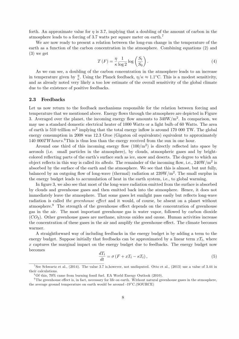
forth. An approximate value for η is 3.7, implying that a doubling of the amount of carbon in theatmosphere leads to a forcing of 3.7 watts per square meter on earth.7

We are now ready to present a relation between the long-run change in the temperature of theearth as a function of the carbon concentration in the atmosphere. Combining equations (2) and(3) we get

T (F ) =η

κ

1

log 2log

(StS0

). (4)

As we can see, a doubling of the carbon concentration in the atmosphere leads to an increasein temperature given by η

κ . Using the Planck feedback, η/κ ≈ 1.1◦C. This is a modest sensitivity,and as already noted very likely a too low estimate of the overall sensitivity of the global climatedue to the existence of positive feedbacks.

2.3 Feedbacks

Let us now return to the feedback mechanisms responsible for the relation between forcing andtemperature that we mentioned above. Energy flows through the atmosphere are depicted in Figure3. Averaged over the planet, the incoming energy flow amounts to 340W/m2. In comparison, wemay use a standard domestic electrical heater of 1000 Watts or a light bulb of 60 Watts. The areaof earth is 510 trillion m2 implying that the total energy inflow is around 170 000 TW. The globalenergy consumption in 2008 was 12.3 Gtoe (Gigaton oil equivalents) equivalent to approximately140 000TWhours.8This is thus less than the energy received from the sun in one hour.

Around one third of this incoming energy flow (100/m2) is directly reflected into space byaerosols (i.e. small particles in the atmosphere), by clouds, atmospheric gases and by bright-colored reflecting parts of the earth’s surface such as ice, snow and deserts. The degree to which anobject reflects in this way is called its albedo. The remainder of the incoming flow, i.e., 240W/m2 isabsorbed by the surface of the earth and the atmosphere. We see that this is almost, but nut fully,balanced by an outgoing flow of long-wave (thermal) radiation at 239W/m2. The small surplus inthe energy budget leads to accumulation of heat in the earth system, i.e., to global warming.

In figure 3, we also see that most of the long-wave radiation emitted from the surface is absorbedby clouds and greenhouse gases and then emitted back into the atmosphere. Hence, it does notimmediately leave the atmosphere. That some gases let sunlight pass easily but reflects long-waveradiation is called the greenhouse effect and it would, of course, be absent on a planet withoutatmosphere.9 The strength of the greenhouse effect depends on the concentration of greenhousegas in the air. The most important greenhouse gas is water vapor, followed by carbon dioxide(CO2). Other greenhouse gases are methane, nitrous oxides and ozone. Human activities increasethe concentration of these gases in the air and amplify the greenhouse effect. The climate becomeswarmer.

A straightforward way of including feedbacks in the energy budget is by adding a term to theenergy budget. Suppose initially that feedbacks can be approximated by a linear term xTt, wherex captures the marginal impact on the energy budget due to feedbacks. The energy budget nowbecomes

dTtdt

= σ (F + xTt − κTt) , (5)

7See Schwartz et al., (2014). The value 3.7 is,however, not undisputed. Otto et al., (2013) use a value of 3.44 intheir calculations.

8Of this, 70% came from burning fossil fuel. EA World Energy Outlook (2010).9The greenhouse effect is, in fact, necessary for life on earth. Without natural greenhouse gases in the atmosphere,

the average ground temperature on earth would be around -19◦C.(SOURCE)

8

Figure 3: Figure 3. Global mean energy budget under present-day climate conditions. Numbersstate magnitudes of the individual energy fluxes in W/m2, adjusted within their uncertainty rangesto close the energy budgets. Numbers in parentheses attached to the energy fluxes cover the rangeof values in line with observational constraints. Source: IPCC (2013), Fig 2.11

where we think of κ as solely determined by the Planck feedback. The steady state temperature isnow given by

T (F ) =η

κ− x1

ln 2ln

(S

S

). (6)

Since the ratio η/(κ−x) has such an important interpretation, it is often labelled the EquilibriumClimate Sensitivity (ECS)10 and we will use the symbol λ to denote it. Some feedbacks are positivebut not necessarily all and theoretically, we cannot rule out neither x < 0 nor x ≥ κ. In the lattercase, dynamics would be explosive which appears inconsistent with historical reactions to naturalvariations in the energy budget. Also x < 0 is diffi cult to reconcile with the observation thatrelatively small changes in forcing in the history of earth has had substantial impact in the climate.However, within these bands a large degree of uncertainty remains.

According to the IPCC, the ECS is “likely in the range 1.5 to 4.5◦C”, “extremely unlikely lessthan 1◦C”, and “very unlikely greater than 6◦C”.11 Another concept, taking some account of theshorter run dynamics, is the Transient Climate Response (TCR). This is the defined as the increasein global mean temperature at the time the CO2 concentration has doubled following a 70 yearperiod of annual increases of 1%.12 IPCC (2013b, Box 12.1) states that the TCR is "likely in therange 1◦C to 2.5◦C" and "extremely unlikely greater than 3◦C."10Note that equilibrium here refers to the energy budget. For an economist, it might have been more natural to

call λ the steady state climate sensitivity.11 (IPCC, 2013a, page 81 and IPCC, 2013b, Box 12.1). The report states that “likely”should be taken to mean a

probability of 66-100%, “extremely unlikely”0-5% and “very unlikely”0-10%.12This is about twice as fast as current increases in the CO2 concentration. Over the 5, 10 and 20 year periods ending

in 2014, the average increase in the CO2 concentration has been 0.54, 0.54 and 0.48 percent per year, respectively.

9

The direct effect on forcing of a given increase in the atmospheric concentration of, e.g., CO2

can be established quite accurately. However, it is much more diffi cult to establish how large anincrease in the average temperature in which this results. As seen in Figure 3, the energy flows arelarge relative to the direct effect of an increase in the concentration of greenhouse gases. Indirecteffects will occur and are typically diffi cult to quantify accurately. For example, an increasedconcentration of CO2 has a direct influence on forcing via the greenhouse effect, but the highertemperature also leads to an increase in air humidity. Water vapor acts as a greenhouse gas andthis amplifies the direct effect. Such an amplification of the direct effect is called a positive feedbackmechanism. Indirect effects may also dampen the initial effect, in which case they are called negativefeedback mechanisms. There are many other feedback mechanisms than water vaporization. Highertemperatures lead to melting icecaps and thereby to a decreasing albedo effect (an ice covered areareflects sunlight better than an area not covered by ice, e.g., water). The formation of cloudsis also of key importance for the energy flows and indirect effects on cloud formation may causeboth positive and negative feedbacks. Because the flows are large relative to the direct effect ofemission of greenhouse gases, just a small error in the calculation of the indirect feedback effectswill have large impacts on the error in the calculation of the overall effect. This is the reason forthe diffi culties in establishing an exact value for climate sensitivity η

κ−x in equation (2).

2.3.1 Feedbacks and uncertainty

It is important to note that the fact that 1κ−x is a non-linear transformation of x has important

consequences for how uncertainty about the strength of feedbacks translate into uncertainty aboutthe equilibrium climate sensitivity.13 Suppose, for example, that the uncertainty about the strengthin the feedback mechanism can be represented by a symmetric triangular density function withmode 2.1 and endpoints at 1.35 and 2.85. This is represented by the upper panel of Figure 4. Themean, and most likely, value of x translates into a climate sensitivity of 3. However, the implieddistribution of climate sensitivities is severely skewed to the right.14 This is illustrated in the lowerpanel, where η

κ−x is plotted with η = 3.7 and κ = 0.3−1.The models have so far assumed linearity. There are obvious arguments in favor of relaxing

this linearity. Changes in the albedo due to shrinking ice sheets and abrubt weaking of the Gulfare possible examples.15 Such effects could simply be introduced by making x in (5) depend ontemperature. This could for example, introduce dynamics with so-called tipping points. Suppose,for example, that

x =

{2.1 if T < 3oC

2.72 else

Using the same parameters as above, this leads to a discontinuity in the climate sensitivity. ForCO2 concentrations below two times S corresponding to a global mean temperature deviation of3 degrees, the climate sensitivity is 3. Above that tipping point, the climate sensitivity is 6. Themapping between St

Sand the global mean temperature using equation (4) is shown in Figure 5.

It is also straightforward to introduce irreversibilities, for example by assuming that feedbacksare stronger (higher x) if a state variable like temperature or CO2 concentration has ever been

However, note that also other greenhouse gases, in particular methane adds to the climate change. For data: seeGlobal Monitor Division of the Earth System Research Labroratory at the U.S. Department of Commerce.13The presentation follows Roe and Baker (2007).14The policy implications of the possibility of a very large climate sensitivity is discussed in Weitzman (2011).15Many state-of-the-art climate models feature regional tipping points, see Drijfhouta at al. (2015) for a list.

Currently, there is, however, no consensus on the existence of specific global tipping points at particular thresholdlevels, see Lenton et al. (2008), Levitan (2013) and IPCC (2013b, section 12.5.5).

10

Figure 4: Figure 4 Example of symmetric uncertainty of feedbacks producing right skewed climatesensitivity.

Figure 5: Figure 5. Tipping point at 3 K due to stronger feedback.

11

Figure 6: Figure 6 Radiative forcing estimates in 2011 relative to 1750 and aggregated uncertaintiesfor the main drivers of climate change. Source: IPCC, Assessment report 5, Summary for policymakers fig 5.

above some threshold value.

2.4 Total Forcing

As noted above, the increase in CO2 concentration is a key factor behind a positive forcing. How-ever, it is not the only factor. In Figure 6, the overall change in the energy budget since thebeginning of the industrial era is decomposed into a number of different components. The size ofthe bars indicate expected contributions to overall forcing and the thin black lines that go throughthe bars indicate a range of uncertainty. We can see that CO2 has the strongest positive effectamong all factors. Other greenhouse gases, including methane and other long-lived gases, as wellas ozone, have a positive effect on forcing. The human influence on land use seems to have had asmall cooling effect. There are also important potential cooling effects that are caused by aerosols,both directly and by aerosols affecting cloud formation in a way that reduces forcing. However,the uncertainty about these effects, in particular about cloud formation, is particularly large. Incomparison to the forcing factors due to humans, the effect of solar irradiance is negligible Thesum of the contribution of all factors to forcing is very likely positive, with a point estimate of 2.29Watts per square meter, but with quite a large range of uncertainty.

2.5 Heating of the oceans

In equation (1), we described a law-of-motion for the atmospheric temperature, i.e. an equationthat describes what happens to the temperature over time for a given level of forcing. The logic

12

behind the equation was that of an energy budget. If the budget is in surplus heat is accumulatedand the temperature increases (and vice versa). The air heats quite quickly but this is not truefor the oceans. Therefore, energy flows between the ocean and the atmosphere may occur andincluding these in the energy budget can improve our analysis. Let us abstract from the regionaldifferences in temperature discussed in the previous section and let Tt and TLt , respectively, denotethe atmospheric and ocean temperature in period t. With two temperatures, we will now haveenergy budgets defined separately for the atmosphere and for the oceans. Furthermore, allow for avariation in forcing over time and let Ft denote the forcing at time t.We then arrive at an extendedversion of equation (1) given by

dTtdt

= σ1

(Ft + xTt − κTt − σ2

(Tt − TLt

)). (7)

Comparing (7) to (1), we see that the term σ2

(Tt − TLt

)is added. This term represents a new

flow in the energy budget (now defined specifically for the atmosphere), namely the net energyflow from the atmosphere to the ocean. To understand this term, note that if the ocean is coolerthan the atmosphere, energy flows from the atmosphere to the ocean. This flow is captured inthe energy budget by the term −σ2

(Tt − TLt

). If Tt > TLt , this flow has a negative impact on the

atmosphere’s energy budget and likewise on the rate of change in temperature in the atmosphere(the LHS). The cooler is the ocean relative to the atmosphere, the larger is the negative impact onthe energy budget.

To complete this dynamic model, we need to specify how the ocean temperature evolves byusing the energy budget of the ocean. If the temperature is higher in the atmosphere than in theoceans, energy will flow to the oceans thus causing an increase in the ocean temperature.16 Writingthis as a (linear) equation gives

dTLtdt

= σ3

(Tt − TLt

). (8)

Equations (7) and (8) together complete the specification of how the temperatures of the at-mosphere and the oceans are affected by a change in forcing.

We can simulate the behavior of the system once we specify the parameters of the system(σ1, σ2, σ3,and κ, all positive) and feed in a sequence of forcing Ft. Before that, we should note afew important things about the system.

First, note that the heat capacity of the atmosphere is low relative to that of the oceans. Thisimplies that a warm atmosphere heats the ocean very slowly and the parameters need to be chosento reflect this. Second, the addition of the ocean temperature affects the dynamics of atmospherictemperature. In particular, it slows down the adjustment process. The ocean acts as a drag byhaving a negative impact on the atmosphere’s energy budget as long as Tt > TLt . But the long-runeffect of a permanent increase in forcing remains identical to that given by equation (4). To seethis, assume that both temperatures have settled down to their long-run values as determined bythe forcing F at some point in time denoted t∞. Call these T (F ) and TL (F ) . By assumption, thendTLtdt = 0 , which from (8) implies that Tt∞ = TLt∞ . Since both temperatures were assumed to havesettled down to their long-run values, T (F ) = TL (F ) . Using this in (7), we see that since bothσ2

(Tt∞ − TLt∞

)= 0 and the left-hand side of (7) are zero, it must be that Ft∞ − (κ− x)Tt∞ = 0.

Thus, T (F ) = Fκ−xremains valid as a description of the long-run implications of a permanent

increase in forcing.

16We disregard direct effects of forcing on the ocean’s energy balance.

13

The model is easily simulated, for example in a spreadsheet program like Open Offi ce Calc. Forthis purpose, we first approximate the differential equations (7) and (8) by a system of differenceequations. Following Nordhaus and Boyer (2000) , we set

Tt − Tt−1 = σ1

(Ft−1 − (κ− x)Tt−1 − σ2

(Tt−1 − TLt−1

))(9)

TLt − TLt−1 = σ3

(Tt−1 − TLt−1

)and use the parameters σ1 = 0.226, σ2 = 0.44, σ3 = 0.02 and (κ − x) = 1.23. Now, the left-handsides are the change in temperature between discrete periods rather than the rate of change incontinuous time.17

The first rows in such a simulation are shown in Table 1. By adding rows in the same fashion,increasing the row number by one for each row (this is done automatically in most spread sheets)we can simulate for any period length. The forcing that is fed into the system is a series of ones inthe last column. In comparison, the temperature dynamics without the "drag" from the oceans isincluded in the last column but one. By feeding in different sequences of forcing, we can experimentwith the simulation model.

Table 1. Temperature dynamicsYear Tt TLt Ft=2010 =0 =0 =1

=1+A2 =B2+0.226*(E2-1.23*B2-0.44*(B2-C2)) =C2+0.02*(B2-C2) =1

=1+A3 =B3+0.226*(E3-1.23*B3-0.44*(B3-C3)) =C3+0.02*(B3-C3) =1

In Figure 7, the lower curve represents the ocean temperature TLt which increases quite slowly.The middle curve is the atmospheric temperature, Tt which increases more quickly. We know thatthe long-run increase in both temperatures is given by 1

κ times the increase in forcing, i.e., by0.75 degrees Celsius. Most of the adjustment to the long-run equilibrium is achieved after a fewdecades for the atmosphere but takes several hundred years for the ocean temperature. Withoutthe dragging effect of the oceans, the temperature increases faster, as shown by the top curve.

2.6 Global Circulation Models

So far, we have abstracted from the fact that incoming and outgoing radiation are not evenlydistributed over the globe. Naturally, the energy flow per unit of area is larger around the equatorthan it is on the poles due to the fact that the average angle between the sun rays and the surfacedecreases with the latitude. This tends to create differences in temperatures at different latitudeswhich cause flows in air and water around the globe which transport heat from the equator towardsthe poles. This is disregarded in the simplest models of climate change discussed above and cantherefore only predict the global mean temperature. In many cases, we also need to make predictionsabout regional climate changes and other parameters of the climate, like precipitation, frequenciesof heavy storms and droughts. For this purpose, global circulation models, which explicitly modelhow flows of air and water transport energy, must be used. Furthermore, global circulation modelsare needed to predict how several of the feedback mechanisms discussed above respond to changesin the global energy budget.

The uneven inflow of energy causes more heating around the equator than elsewhere. As aconsequence, the air around the equator becomes moist and warm. The warm and moist air rises,forming clouds, and flows to higher latitudes where it is once more cooled down and falls to the17The timing assumptions for the right-hand sides may seem somewhat arbitrary but follow the principle that

endogenous variables (i.e., those that are determined within the system) on the right-hand side are measured at t−1.

14

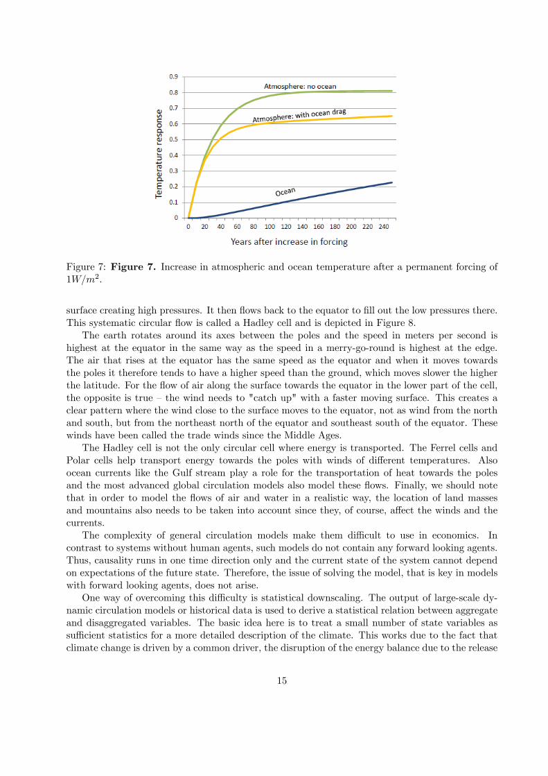
Figure 7: Figure 7. Increase in atmospheric and ocean temperature after a permanent forcing of1W/m2.

surface creating high pressures. It then flows back to the equator to fill out the low pressures there.This systematic circular flow is called a Hadley cell and is depicted in Figure 8.

The earth rotates around its axes between the poles and the speed in meters per second ishighest at the equator in the same way as the speed in a merry-go-round is highest at the edge.The air that rises at the equator has the same speed as the equator and when it moves towardsthe poles it therefore tends to have a higher speed than the ground, which moves slower the higherthe latitude. For the flow of air along the surface towards the equator in the lower part of the cell,the opposite is true —the wind needs to "catch up" with a faster moving surface. This creates aclear pattern where the wind close to the surface moves to the equator, not as wind from the northand south, but from the northeast north of the equator and southeast south of the equator. Thesewinds have been called the trade winds since the Middle Ages.

The Hadley cell is not the only circular cell where energy is transported. The Ferrel cells andPolar cells help transport energy towards the poles with winds of different temperatures. Alsoocean currents like the Gulf stream play a role for the transportation of heat towards the polesand the most advanced global circulation models also model these flows. Finally, we should notethat in order to model the flows of air and water in a realistic way, the location of land massesand mountains also needs to be taken into account since they, of course, affect the winds and thecurrents.

The complexity of general circulation models make them diffi cult to use in economics. Incontrast to systems without human agents, such models do not contain any forward looking agents.Thus, causality runs in one time direction only and the current state of the system cannot dependon expectations of the future state. Therefore, the issue of solving the model, that is key in modelswith forward looking agents, does not arise.

One way of overcoming this diffi culty is statistical downscaling. The output of large-scale dy-namic circulation models or historical data is used to derive a statistical relation between aggregateand disaggregated variables. The basic idea here is to treat a small number of state variables assuffi cient statistics for a more detailed description of the climate. This works due to the fact thatclimate change is driven by a common driver, the disruption of the energy balance due to the release

15

Figure 8: Figure 8 A Hadley cell

16

of green house gases, in particular CO2.Let Ti,t denote a particular measure of the climate, e.g., the yearly average temperature, in

region i in period t. We can then estimate a model like

Ti,t = Ti + f (li, ψ1)Tt + zi,t

zi,t = ρzi,t−1 + νi,t

var (νi,t) = g (li, ψ2)

corr (νi,t, νj,t) = h (d (li, lj) , ψ3)

Here, Ti is the baseline temperature in region i. f, g,and g are specified functions parameterizedby ψ1, ψ2 and ψ3. zi,t is the prediction error that follows and AR1 process. li is some observedcharacteristic of the region, e.g., latitude and d (li, lj) is a distance measure. Krusell and Smith(2015) estimate such a model on historical data. Figure 9 shows the estimated function f withli denoting latitude. We see that an increase in the global mean temperature Tt has an effect onregional temperature levels that depends strongly on the latitude. The effect of a one degree Celsiusincrease in the global temperature ranges from 0.25 to 3.6 degrees. Figure 9 shows the correlationpattern of prediction errors using d to measure Euclidian distance.

2.7 Historical climate

Looking back around 500 million years in time (which equals around 10 % of the age of the earth),there are actually ways of making statements about how the climate has changed. Naturally, nodirect measurements can be used, i.e. scientists have to fall back on proxy methods. A proxyvariable is a measurable variable that is known to be correlated with the variable of interest.Usually, proxy data from tree rings, corals, plankton and pollen and other such sources, are appliedto draw conclusions about the nature of the climate in the past. Essentially, we can say that theclimate has been much warmer in the past than it is today. In the IPCC report of 2007, Solomon

17

Figure 9: Figure 9

et al. state that “during most of the past 500 million years, earth was probably completely free ofice sheets”.18

While proxy data constitute the only tool for estimations of past temperatures, atmosphericgas concentrations over the last 650,000 years can actually be measured. These measures aredone from bubbles of air that have been trapped in arctic ice cores over the years. Greenhousegas concentrations can be measured in those air bubbles and conclusions can be drawn aboutatmospheric greenhouse gas concentrations during the past centuries.

Figure 10 shows how the concentrations of the three important greenhouse gases carbon dioxide,methane and nitrous oxide have varied over the last 650,000 years. Furthermore, the graph alsoincludes a curve called δD which is used as a proxy for the temperature.19 The five gray bars inthe graph indicate interglacial periods. Consequently, the white parts in between reflect ice ages.At the moment, we are living in a period between two ice ages. No worries, conditions that maytrigger the next ice age will likely not exist for at least the next 30,000 years.

As shown in the figure, the greenhouse gas is closely correlated with temperatures (as proxiedby δD). However, the temperature tends to increase before the increase in greenhouse gas con-centrations. This, in turn, means that a higher atmospheric CO2 concentration is not the factorthat triggers the turn from a glacial to an interglacial period but, instead, CO2 concentrationsrise in response to an increase in the temperature. It is not yet quite clear where this causalityhas its origin but a reasonable interpretation is that this is an example of a positive feedback inworking. Something caused an increase in the global temperature, this lead to an increase in CO2

concentration in the atmosphere, which further increased the temperature.Even though it has not been fully resolved among scientists, we can assume that the mechanism

behind the glacial-interglacial cycles on the one hand is a mechanism of variations in how elliptical

18 IPCC, 2007, FAQ 6.119The δD measure uses the fact that a small share of the hydrogen in ocean water is deuterium (hydrogen with an

extra neutron). Such heavy water has lower vapor pressure and the concentration of heavy water in rainfall can beused to proxy for temperature.

18

Figure 10: Figure 10 Greenhouse gas concentrations over the last 650,000 years.

(eccentric) is the earth’s orbit around the sun and of variations in the tilt of the earth’s axis relativeto its path around the sun, on the other hand. These orbital changes are called Milankovitch cyclesand appear to be correlated with slow changes in the global climate. The Milankovitch cyclesimply variations in the distribution of sunlight over the globe and can therefore cause changes inthe climate. A decisive trigger at the beginning of an ice age may occur when solar radiation duringthe summer is no longer strong enough to reduce the snow and ice layers in the northern hemispherethat are accumulated during the winter. If this is the case, the blanket of snow can be aggregatedover the years which leads to a larger reflection of sunlight from the surface of the earth due to thehigher albedo of snow and ice. Such a positive ice-albedo feedback reinforces the initial reduction inthe incoming energy flow and an ice age can get started. When the conditions are instead such thatsummers in the northern hemisphere become warmer, the glaciers start to melt and an interglacialperiod is about to start. As mentioned above, carbon dioxide concentrations also tend to risewith increasing temperatures. The result is another positive feedback effect. The consequence isfeedback effects that are strong enough so that only small variations in solar radiation due to theMilankovitch cycle can cause transitions between ice ages and interglacial periods.

Naturally, a change in received solar radiation on earth is not necessarily caused by a changeof the earth’s orbit and the obliquity of its axis. Moreover, the energy output of the sun itself isnot always equal but varies in cycles and also over longer terms. This variations as well as otherfactors that are not caused by human beings (such as, for instance, the activity of volcanoes) havean influence on the climate over the centuries.

2.8 More recent changes in the climate

Before the mid 19th century, instrumental records of the temperature are not suffi ciently availableto allow a re-construction of the global temperature. Instead, various proxies are used, leading todifferent results depending on the method chosen. However, a reasonable conclusion from judgingthe overall evidence is that the middle of both the first and second millennium AD was colder than

19

­0.6

­0.4

­0.2

­0.0

0.2

0.4

0.6

Tem

pera

ture

 ano

mal

y (°

C)

­0.6

­0.4

­0.2

­0.0

0.2

0.4

0.6

Tem

pera

ture

 ano

mal

y (°

C)

­0.6

­0.4

­0.2

­0.0

0.2

0.4

0.6

Tem

pera

ture

 ano

mal

y (°

C)

1860 1880 1900 1920 1940 1960 1980 2000­0.6

­0.4

­0.2

­0.0

0.2

0.4

0.6

Tem

pera

ture

 ano

mal

y (°

C)

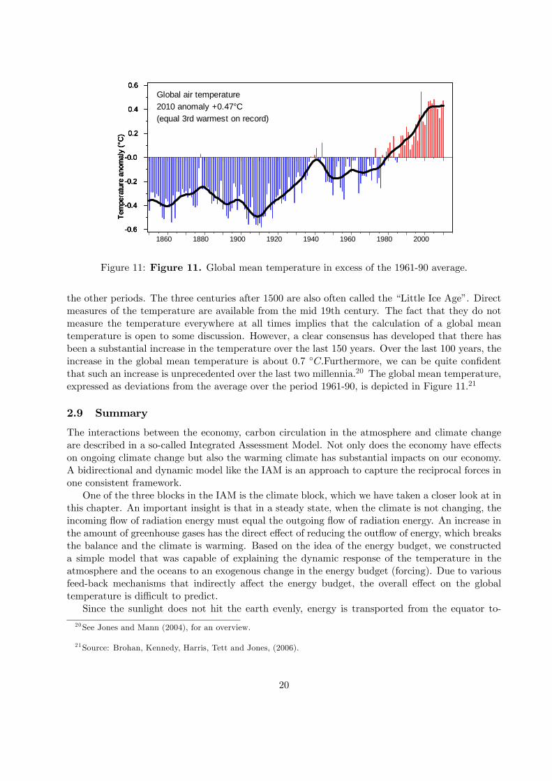
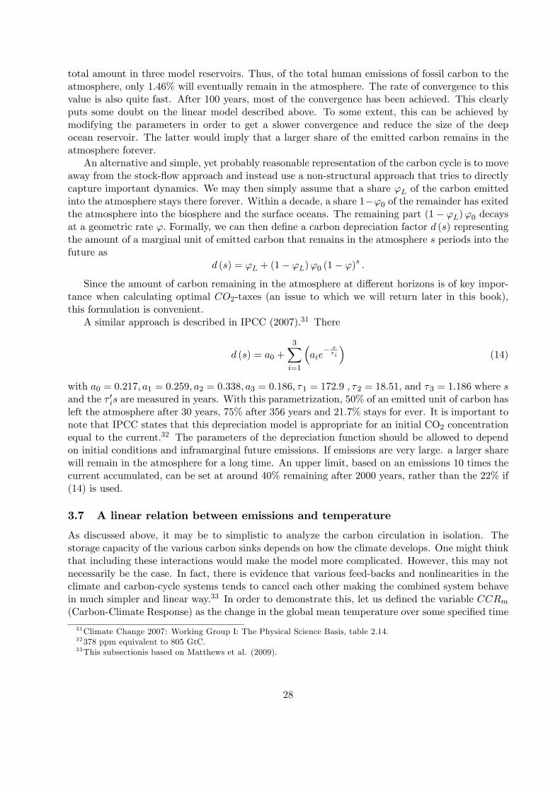
Global air temperature2010 anomaly +0.47°C(equal 3rd warmest on record)

Figure 11: Figure 11. Global mean temperature in excess of the 1961-90 average.

the other periods. The three centuries after 1500 are also often called the “Little Ice Age”. Directmeasures of the temperature are available from the mid 19th century. The fact that they do notmeasure the temperature everywhere at all times implies that the calculation of a global meantemperature is open to some discussion. However, a clear consensus has developed that there hasbeen a substantial increase in the temperature over the last 150 years. Over the last 100 years, theincrease in the global mean temperature is about 0.7 ◦C.Furthermore, we can be quite confidentthat such an increase is unprecedented over the last two millennia.20 The global mean temperature,expressed as deviations from the average over the period 1961-90, is depicted in Figure 11.21

2.9 Summary

The interactions between the economy, carbon circulation in the atmosphere and climate changeare described in a so-called Integrated Assessment Model. Not only does the economy have effectson ongoing climate change but also the warming climate has substantial impacts on our economy.A bidirectional and dynamic model like the IAM is an approach to capture the reciprocal forces inone consistent framework.

One of the three blocks in the IAM is the climate block, which we have taken a closer look at inthis chapter. An important insight is that in a steady state, when the climate is not changing, theincoming flow of radiation energy must equal the outgoing flow of radiation energy. An increase inthe amount of greenhouse gases has the direct effect of reducing the outflow of energy, which breaksthe balance and the climate is warming. Based on the idea of the energy budget, we constructeda simple model that was capable of explaining the dynamic response of the temperature in theatmosphere and the oceans to an exogenous change in the energy budget (forcing). Due to variousfeed-back mechanisms that indirectly affect the energy budget, the overall effect on the globaltemperature is diffi cult to predict.

Since the sunlight does not hit the earth evenly, energy is transported from the equator to-

20See Jones and Mann (2004), for an overview.

21Source: Brohan, Kennedy, Harris, Tett and Jones, (2006).

20

wards the poles with winds and water. To predict the regional distribution of climate change andother factors of the climate like precipitation and storm frequencies and analyze various feedbackmechanisms like cloud formation, these flows need to be modeled in global circulation models.

3 Carbon circulation

As discussed in the introduction, an Integrated Assessment Model contains three blocks; the climate,the carbon circulation and the economy. In the previous chapter, we took a closer look at theclimate, the energy budget on earth and a very simple climate model. In this chapter, we will takea closer look at the second block, the carbon circulation, and how to model it for our purposes.

3.1 The stock-flow approach

Burning of fossil fuel leads to emissions of carbon dioxide into the atmosphere. These emissionsare very likely to be the largest of all human contributions to climate change. In order to forecastclimate change and, for example, calculate the value of the damages caused by emission, we needto understand how the atmospheric concentration of CO2 is related to past emissions. For thispurpose, we will first have a look at a carbon circulation model based on the stock-flow approach.The first fundamental ingredients in the model are the stocks of carbon, which we call carbonreservoirs. In Figure 12, the carbon reservoirs are represented by boxes. The number in black ineach box indicates the size of the reservoir in GtC, i.e., billions of tons of carbon. As we can see,the biggest reservoir by far is the Intermediate/deep ocean, with more than 37,000 Gigatons ofcarbon. Vegetation and the atmosphere are of about the same size although the uncertainty aboutthe former is substantial. Soils represent a larger stock as do carbon embedded in the permafrost.

Before turning to the red figures, let us describe the second ingredient of the model, the flows.Black arrows in Figure 12 indicate pre-industrial flows between the stocks measured in GtC peryear. In the figure, we can see that for some black arrows from a given reservoir, we find an opposedarrow (or a sum of opposed arrows) that transports similar amounts of carbon back to the givenreservoir. So for example, flows between the atmosphere and the ocean was almost balanced. Withzero net flows between the stocks, the latter remain constant in size over time. Here, it may beconvenient to note the analogy with the model of the energy budget. When net flows of energybetween different sub-systems are zero, the heat content and thus the temperature remain constant.

Let us now look more closely at some of the flows between reservoirs. By transforming carbondioxide into organic substances, vegetation in the earth’s biosphere induces a flow of carbon fromthe atmosphere to the biosphere. This process is well-known as photosynthesis. The reverse process,respiration, is also taking place in plants’fungi, bacteria and animals. This, together with oxidation,fires and other physical processes in the soil, leads to the release of carbon in the form of CO2 to theatmosphere. A similar process is taking place in the sea, when carbon is taken up by phytoplanktonin the sea through photosynthesis and released back into the surface ocean. When phytoplanktonsink into deeper layers they take carbon with them. A small fraction of the carbon that is sinkinginto the deep oceans is eventually buried in the sediments of the ocean floor, but most of thecarbon remains in the circulation system between lower and higher ocean water. Between theatmosphere and the upper ocean, CO2 is directly exchanged. Carbon dioxide reacts with waterand forms dissolved inorganic carbon that is stored in the water. When the CO2 rich surface watercools down in the winter, it falls to the deeper ocean and a similar exchange occurs in the otherdirection. From the figure, we also note that there are large flows of carbon between the upperlayers of the ocean and the atmosphere via gas exchange. These flows are smaller, but of the same

21

Figure 12: Figure 12. Global carbon cycle. Stocks in GtC (PgC) and flows GtC/year. Source:IPCC (2013), Figure 6.1.

22

order of magnitude as the photosynthesis and respiration. We note that there is a bet flow fromthe atmosphere to the oceans.

3.2 Human Influence on Carbon Circulation

Before the industrial revolution, human influence on carbon circulation was small. However, at-mospheric CO concentration started to rise from the mid 18th century and onwards, mainly due tothe burning of fossil fuels and deforestation but also as a result of rising cement production. Otherhuman factors that affect the concentration of carbon dioxide in the atmosphere are the burningof biomass and the conversion of grasslands or forests to croplands.

In Figure 12, the red figures denote changes in the reservoirs and flows over and above pre-industrial values. The figures for reservoirs refer to 2011 while flows are yearly averages duringthe period 2000-2009. At the bottom of the picture, we see that the stock of fossil fuel in theground has been depleted by 365 ± 30 GtC since the beginning of industrialization. The flow tothe atmosphere due to fossil fuel use and cement production is reported to 7.8± 0.6 GtC per year.In addition, changed land use adds 1.1± 0.8 GtC per year to the flow of carbon to the atmosphere.In the other direction, the net flows from the atmosphere and to the terrestial biosphere and to theoceans have increased. All in all, we note that while the fossil reserves have shrunk, the amount ofcarbon in atmosphere has gone from close to 600 to around 840 GtC and currently increases at arate of 4 GtC per year. A sizeable but somewhat smaller increase has increased in the oceans whilethe amount of carbon in vegetation has remained largely constant.

Again in close analogy with the energy budget, we see that the gross flows of carbon are largerelative to the additions due to fossil fuel burning. Furthermore, the flows may be indirectlyaffected by climate change. For example, the ability of the biosphere to store carbon is affected bytemperature and precipitation. Similarly, the ability of the oceans to store carbon is affected bythe temperature. Deposits of carbon in the soil may also be affected by climate change. We willreturn to these mechanisms below.

3.3 Size of fossil reserves

The extent to which burning of fossil fuel is a problem from the perspective of climate change ob-viously depends on how much fossil fuel remains to burn. This amount is not known and estimatesdepends on definitions. The amount of fossil resources that eventually can be used depends onestimates of future findnings as well as on forecasts about technological developments and relativeprices. Often, reserves are defined in successively wider classes. For example, the U.S. EnergyInformation Agency defines four classes for oil and gas. The smallest is proved reserves, which arereserves that geologic and engineering data demonstrate with reasonable certainty to be recover-able in future years from known reservoirs under existing economic and operating conditions. Astechnology and prices change, this stock normally increases over time. Succesively larger ones areeconomically recoverable resources, technically recoverable resources and remaining oil and naturalgas in-place.

Given different definitions and estimation procedures the estimated stocks differ and will changeover time. Therefore, the numbers in this section can only be taken as indications. Furthermore,reserves of different types of fossil fuels are measured in different units, often barrels for oil, cubicmeters or cubic feet for gas and ton for coal. However, for our purpose, it is convenient to expressall stocks in terms of their carbon content. Therefore non-trivial conversion must be undertaken.Given these caveats, we calculate from BP (2015) global proved reserves of oil and natural gas to

23

be approximately 200 GtC and 100 GtC, respectively.22 At current extraction rates, both thesestocks would last approximately 50 years. Putting this numbers in perspective, we note that theatmosphere currently contains over 800 GtC. Given the results in the previous sections, we note thatburning all proved reserves of oil and natural gas would have fairly modest effects on the climate.23

Again using BP (2015), we calculate proved reserves of coal to around 600 GtC, providing morepotential dangers for the climate.

Using wider definitions of reserves, stocks are much larger. Specifically, using data from Mcgladeans Ekins (2015) we calculate ultimately recoverable reserves of oil, natural gas and coal to closeto 600 GtC, 400 GtC and 3000 GtC.24 Rogner (1997), estimates coal reserves to be 3,500GtC witha marginal extraction cost curve that is fairly flat. Clearly, if all these reserves are used, climatechange can hardly be called modest.

3.4 A Linear Carbon Circulation Model

Let us now construct a very simple carbon circulation model using the stock-flow approach. Toprepare for an implementation in a spread-sheet program, we will write the model in discrete time.Let us begin with a two-stock model, where the variables St and SLt denote the amount of carbonin the two reservoirs, respectively. Let us think of St as the atmosphere and SLt as the ocean, fornow abstracting from the other reservoirs. Emissions, denoted Mt, enter into the atmosphere. Wealso need to model the flows between reservoirs. For simplicity, let us assume that a constant shareφ1 of St flows to S

Lt in every period and, conversely, a share φ2 of S

Lt flows in the other direction.

The change in the amount of carbon in the atmosphere between periods t and t− 1 is then the netflow. This can be written as the following equation

St − St−1 = −φ1St−1 + φ2SLt−1 +Mt−1. (10)

The left-hand side is the change in the amount of carbon in the atmosphere, and the right-handside is the net flow during the previous period, consisting of i) the outflow to the ocean (−φ1St−1),ii) the inflow from the ocean (φ2S

Lt−1) and iii) emission Mt−1.

We can construct a similar equation for the amount of carbon in the ocean;

SLt − SLt−1 = φ1St−1 − φ2SLt−1. (11)

As we can see, equations (10) and (11) form a linear system of difference equations, quite similarin structure to equation (9). However, there is a key difference; additions of carbon to this systemthrough emissions get "trapped" in the sense that there is no outflow from the system as a whole.25

This implies that if M settles down to a positive constant, the sizes of reservoirs S and SL will notapproach a steady state, but will grow for ever. If, emissions eventually stop and remain zero, the

22BP (2015) reports proved oil reserves to 239,8 Gt. For conversion, we use IPCC (2006), table 1.2 and 1.3. Fromthese, we calculate a carbon content of 0.846 GtC per Gt of oil. BP (2015) reports proved natural gas reserves to187.1 trillion m3.The same source states an energy content of 35.7 trillion BtU per trillion m3equal to 35. 9 trillionkJ. IPCC (2006) reports 15.3 kgC/GJ for natural gas. This means that 1 trillion m3 natural gas contains 0.546 GtC.For coal, we use the IPCC (2006) numbers for antracit, giving 0.716 GtC per Gt of coal. For all these conversions,it should be noted that there is substantial variation in carbon content depending on the quality of the fuel and thenumbers used must therefore be used with suffi cient caution.23As we will soon see, a substantial share of burned fossil fuel quickly leaves the atmosphere.24See previous footnote for conversions.25 If we were to define also a stock of fossil fuel in ground from which emmissions were taken, total net flows would

be zero. Since it is safe to assume that flows to the stock of fossil fuel is neglible, we could simply add an equationRt = Rt−1 −Mt−1 to the others which would capture the depletion of fossil reserves.

24

sizes of the reservoirs will settle down to some steady-state values, but these values will dependon what amount of emissions have been accumulated before that.26 However, without any furtherinformation about the history of emissions, we can calculate the relative size of the two reservoirsin steady state. Let us denote steady states by omitting the time subscript. Setting the RHS of(10) to zero for zero emissions and assuming the system is in steady state then yields

0 = −φ1S + φ2SL (12)

which can be rewritten asS

SL=φ2

φ1

.

An alternative way of deriving this result is to note that in a steady state, it must be the casethat the flows to and from each reservoir must be the same. Clearly if the flow into the atmosphere,for example, is larger (smaller) than the outflow, the amount of carbon in the atmosphere mustbe growing (shrinking). Noting that the inflow to the atmosphere in steady state is φ2S

L and theoutflow φ1S we get φ1S = φ2S

L which is equivalent to (12)Thus, if emissions stop, the ratio of the stocks eventually approach a constant, given by the

parameters of the system. We argued above that carbon circulation was approximately in a steadystate before fossil fuel burning started. Specifically, we then had 589 GtC in the atmosphere and37,100 GtC in oceans, yielding a ratio of approximately 1.59%. Regardless of how much carbonis released into the atmosphere, our simplified model implies that, eventually, this ratio will berestored.

We can also use this ratio to calibrate our model; notwithstanding what value we set for φ1 weshould set φ2φ1 = 1.59%. Now, what value should we choose for φ1? Let us think about how different

values of φ1 affect the dynamics. Suppose that we set φ1 to quite a large value.27 Then, flows

are large relative to the stocks and the system quickly adjusts to a steady state after a period ofemissions. If instead φ1 is very small, flows are small and it takes a long time before the systemsettles down. We may then calibrate the model by choosing a value of φ1 that implies a reasonablespeed of convergence.

BOX 1The linear systems (10) and (11) can be solved exactly. Suppose that Mt+s = 0 for

all s ≥ 0, given some fixed t. Then, it is straightforward to show that for all s ≥ 0,

St+s = φ2φ1+φ2

(St + SLt

)− φ2S

Lt −φ1Stφ1+φ2

(1− φ1 − φ2)s

SLt+s = φ1φ1+φ2

(St + SLt

)+

φ2SLt −φ1Stφ1+φ2

(1− φ1 − φ2)s .

The equations show that the sum of carbon is constant (there is a unit root in thesystem). Furthermore, the term φ2S

Lt −φ1Stφ1+φ2

(1− φ2 − φ1)s determines the convergence.As s approaches infinity, these terms vanish and the stocks of carbon approach theratio φ2

φ1. The rate of convergence is determined by the sum of the flow parameters

(the roots of the system are (1− φ1 − φ2) and 1). Specifically, the closer this sum is tounity, the quicker is the convergence.26Mathematically, we say that the dynamic system has a unit root.27But it cannot be larger than unity. Why?

25

3.5 Carbon circulation in a DICE-type model

In the DICE models developed by Nordhaus, the representation of the carbon cycle has threereservoirs. St represents the atmosphere in period t, SUt is the surface ocean combined with theterrestrial biosphere, and finally SLt , which represents the deep oceans. As in the two-stock case,discussed in the previous subsection, the flows of carbon between these reservoirs are assumed tobe constant fractions of the sizes of the reservoirs expressed by coeffi cients φij,. The flow fromreservoirs i to stock j is thus φijS

it .

The Nordhaus DICE carbon circulation can then be written

St − St−1 = −φ12St−1 + φ21SUt−1 +Mt−1 (13)

SUt − SUt−1 = φ12St−1 − (φ21 + φ23)SUt−1 + φ32SLt−1

SLt − SLt−1 = φ23SUt−1 − φ32S

Lt−1.

Note that for every reservoir, all inflows (except emissions) must equal an outflow from anotherstock. For example, the inflow to the surface ocean from the atmosphere is φ12St−1 which is thefirst term in the equation for the change of the size of upper ocean (the middle equation in (13)).The same term but with an opposite sign appears as the first term in in the first equation whereit represents the outflow from the atmosphere to the surface ocean. The fact that all outflows areinflows to other reservoirs means that carbon can be transported between the three stocks but nocarbon can be lost during the process of exchange. If emissions stop, the sum of carbon in thethree reservoirs therefore remains constant for all time. Atmospheric carbon can either stay in theatmosphere or be taken up by the ocean top layer or the biosphere. Carbon in the top layer of theocean or in the biosphere can either stay there, be given back to the atmosphere or be taken intodeeper ocean layers. The carbon in the deep ocean can remain there or be carried up to higherlayers by circulation.

With a little creativeness, we can use Figure 12 to calibrate the parameters of the system.28 Infact, we can do this in several ways. There are four parameters that needs to be given numericalvalues, so we need to use (at least) four pieces of information from the figure. Let’s start with φ12 ,which determines the flow from the atmosphere to the surface ocean. Let us for now disregardvegetation (we will return to that later). Then we note from figure 12 that the pre-industrial flowfrom was 60 and the stock of carbon in the atmosphere was 589. Thus, we set

φ12 =60

589≈ 0.102.

Then, let us use that the carbon circulation system was in a steady state (approximately) beforeindustrialization.29 This means that the flow into the atmosphere equals the flow out of the at-mosphere. Thus, we set the inflow to 60 and note that the inflow is given by φ21S

Ut−1. Since the

stock was 900, this gives us

60 = φ21900⇒ φ21 =60

900≈ 0.0667.

In an exactly analogous way, we use the piece of information that the flow from surface oceanto the deep ocean was 90 out of a stock of 900, giving φ23 = 90

900 = 0.100. Finally, the flow back

28An alternative route, followed by Nordhaus, is to calibrate the model so that it replicates the behavior of a moreelaborate model as well as possible.29 In the figure, this is not exactly true. Specifically, the inflow to the atmosphere from the surface ocean is 60.7,

rather than 60. However, we disregard this small discrepancy.

26

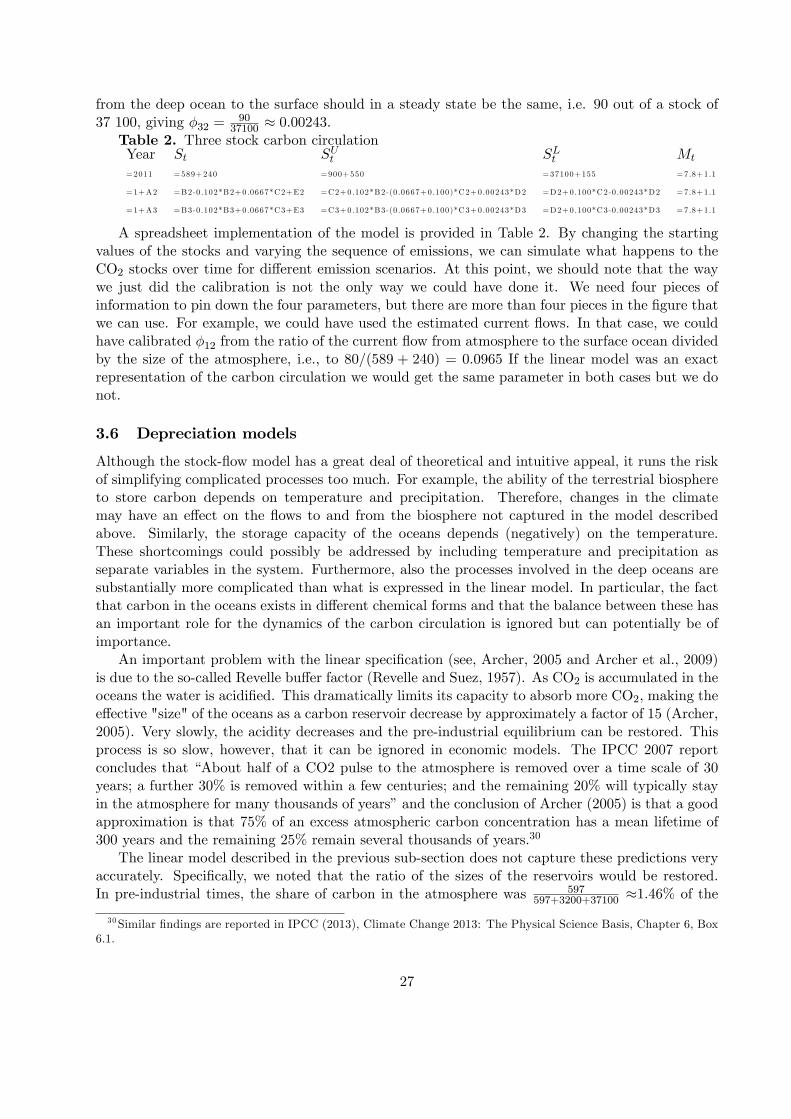
from the deep ocean to the surface should in a steady state be the same, i.e. 90 out of a stock of37 100, giving φ32 = 90

37100 ≈ 0.00243.Table 2. Three stock carbon circulationYear St SUt SLt Mt

=2011 =589+240 =900+550 =37100+155 =7.8+1.1

=1+A2 =B2-0.102*B2+0.0667*C2+E2 =C2+0.102*B2-(0 .0667+0.100)*C2+0.00243*D2 =D2+0.100*C2-0.00243*D2 =7.8+1.1

=1+A3 =B3-0.102*B3+0.0667*C3+E3 =C3+0.102*B3-(0 .0667+0.100)*C3+0.00243*D3 =D2+0.100*C3-0.00243*D3 =7.8+1.1

A spreadsheet implementation of the model is provided in Table 2. By changing the startingvalues of the stocks and varying the sequence of emissions, we can simulate what happens to theCO2 stocks over time for different emission scenarios. At this point, we should note that the waywe just did the calibration is not the only way we could have done it. We need four pieces ofinformation to pin down the four parameters, but there are more than four pieces in the figure thatwe can use. For example, we could have used the estimated current flows. In that case, we couldhave calibrated φ12 from the ratio of the current flow from atmosphere to the surface ocean dividedby the size of the atmosphere, i.e., to 80/(589 + 240) = 0.0965 If the linear model was an exactrepresentation of the carbon circulation we would get the same parameter in both cases but we donot.

3.6 Depreciation models

Although the stock-flow model has a great deal of theoretical and intuitive appeal, it runs the riskof simplifying complicated processes too much. For example, the ability of the terrestrial biosphereto store carbon depends on temperature and precipitation. Therefore, changes in the climatemay have an effect on the flows to and from the biosphere not captured in the model describedabove. Similarly, the storage capacity of the oceans depends (negatively) on the temperature.These shortcomings could possibly be addressed by including temperature and precipitation asseparate variables in the system. Furthermore, also the processes involved in the deep oceans aresubstantially more complicated than what is expressed in the linear model. In particular, the factthat carbon in the oceans exists in different chemical forms and that the balance between these hasan important role for the dynamics of the carbon circulation is ignored but can potentially be ofimportance.

An important problem with the linear specification (see, Archer, 2005 and Archer et al., 2009)is due to the so-called Revelle buffer factor (Revelle and Suez, 1957). As CO2 is accumulated in theoceans the water is acidified. This dramatically limits its capacity to absorb more CO2, making theeffective "size" of the oceans as a carbon reservoir decrease by approximately a factor of 15 (Archer,2005). Very slowly, the acidity decreases and the pre-industrial equilibrium can be restored. Thisprocess is so slow, however, that it can be ignored in economic models. The IPCC 2007 reportconcludes that “About half of a CO2 pulse to the atmosphere is removed over a time scale of 30years; a further 30% is removed within a few centuries; and the remaining 20% will typically stayin the atmosphere for many thousands of years”and the conclusion of Archer (2005) is that a goodapproximation is that 75% of an excess atmospheric carbon concentration has a mean lifetime of300 years and the remaining 25% remain several thousands of years.30

The linear model described in the previous sub-section does not capture these predictions veryaccurately. Specifically, we noted that the ratio of the sizes of the reservoirs would be restored.In pre-industrial times, the share of carbon in the atmosphere was 597

597+3200+37100 ≈1.46% of the

30Similar findings are reported in IPCC (2013), Climate Change 2013: The Physical Science Basis, Chapter 6, Box6.1.

27

total amount in three model reservoirs. Thus, of the total human emissions of fossil carbon to theatmosphere, only 1.46% will eventually remain in the atmosphere. The rate of convergence to thisvalue is also quite fast. After 100 years, most of the convergence has been achieved. This clearlyputs some doubt on the linear model described above. To some extent, this can be achieved bymodifying the parameters in order to get a slower convergence and reduce the size of the deepocean reservoir. The latter would imply that a larger share of the emitted carbon remains in theatmosphere forever.

An alternative and simple, yet probably reasonable representation of the carbon cycle is to moveaway from the stock-flow approach and instead use a non-structural approach that tries to directlycapture important dynamics. We may then simply assume that a share ϕL of the carbon emittedinto the atmosphere stays there forever. Within a decade, a share 1−ϕ0 of the remainder has exitedthe atmosphere into the biosphere and the surface oceans. The remaining part (1− ϕL)ϕ0 decaysat a geometric rate ϕ. Formally, we can then define a carbon depreciation factor d (s) representingthe amount of a marginal unit of emitted carbon that remains in the atmosphere s periods into thefuture as

d (s) = ϕL + (1− ϕL)ϕ0 (1− ϕ)s .

Since the amount of carbon remaining in the atmosphere at different horizons is of key impor-tance when calculating optimal CO2-taxes (an issue to which we will return later in this book),this formulation is convenient.

A similar approach is described in IPCC (2007).31 There

d (s) = a0 +

3∑i=1

(aie− sτi

)(14)

with a0 = 0.217, a1 = 0.259, a2 = 0.338, a3 = 0.186, τ1 = 172.9 , τ2 = 18.51, and τ3 = 1.186 where sand the τ ′is are measured in years. With this parametrization, 50% of an emitted unit of carbon hasleft the atmosphere after 30 years, 75% after 356 years and 21.7% stays for ever. It is important tonote that IPCC states that this depreciation model is appropriate for an initial CO2 concentrationequal to the current.32 The parameters of the depreciation function should be allowed to dependon initial conditions and inframarginal future emissions. If emissions are very large. a larger sharewill remain in the atmosphere for a long time. An upper limit, based on an emissions 10 times thecurrent accumulated, can be set at around 40% remaining after 2000 years, rather than the 22% if(14) is used.

3.7 A linear relation between emissions and temperature

As discussed above, it may be to simplistic to analyze the carbon circulation in isolation. Thestorage capacity of the various carbon sinks depends on how the climate develops. One might thinkthat including these interactions would make the model more complicated. However, this may notnecessarily be the case. In fact, there is evidence that various feed-backs and nonlinearities in theclimate and carbon-cycle systems tends to cancel each other making the combined system behavein much simpler and linear way.33 In order to demonstrate this, let us defined the variable CCRm(Carbon-Climate Response) as the change in the global mean temperature over some specified time

31Climate Change 2007: Working Group I: The Physical Science Basis, table 2.14.32378 ppm equivalent to 805 GtC.33This subsectionis based on Matthews et al. (2009).

28

interval m per unit of emissions of fossil carbon into the atmosphere over that same time interval

CCR ≡ Tt+m − Tt∑t+m−1s=t Ms

.

The numerator is the change in global mean temperature over the time interval t to t + m.The denominator is total accumulated carbon emissions over the same time interval. Given ourprevious discussion in this and the previous chapter, one would think that this variable is far froma constant. The dynamic behavior of the climate and the carbon cycle could make CCRm dependon the length of the time interval considered. For example, since it takes time to heat the oceans,the temperature response could depend on whether the time interval over which we measure is adecade or a century. Similarly, since also the carbon dynamics is slow, the extra CO2-concentrationinduced by a unit of emission tends to be lower the longer the time interval considered. Furthermore,CCRm might depend on how much emissions have already occurred. Higher previous emissions canreduce the effectiveness of carbon sinks and even turn them into net contributors. The marginaleffect on temperature from an increase in the CO2-concentration also depends on the level of CO2

concentration.Quite surprisingly, Matthews et al. (2009) show that all these dynamic and non-linear effects

tend to cancel, making it a quite good approximation that CCRm is a constant, independent ofboth the time interval considered and the amount of previous emissions. Of course, there areuncertainties about the value of CCR. Matthews et al. (2009) pin down the uncertainty, arguingthat a 95% confidence interval is between 1 and 2.1 degrees Celsius per 1000 GtC. Both modelsimulations and historical data suggest a best estimate of approximate one and a half degreeswarming per 1000 GtC. This means that we can write the (approximate) linear relationship

Tt+m = Tt + CCRt+m−1∑s=t

Ms

To get some understanding for this surprising result, first consider the time independence. Wehave shown in the previous chapter that when the ocean is included in the analysis, there is asubstantial delay in the temperature response of a given forcing. Thus, if the CO2-concentrationpermanently jumps to a higher level, it takes many decades before even half the final change intemperature has occurred. On the other hand, if carbon is released into the atmosphere, a largeshare of if is removed quite slowly from the atmosphere. It happens to be the case that thesedynamics cancel each other, at least if the time scale is from a decade up to a millennium. Thus,in the shorter run, the CO2 concentration and thus forcing is higher but this is balanced by thecooling effect of the oceans.

Second, for the independence of CCR with respect to previous emissions note that the Arrenhiuslaw discussed in the previous chapter implies a logarithmic relation between CO2 concentration andthe temperature. Thus, at higher CO2 concentrations, an increase in the CO2 concentration hasa smaller effect on the temperature. On the other hand, existing carbon cycle models tends tohave the property that the storage capacity of the sinks diminish as more CO2 is released intothe atmosphere. These effects also balance – at higher levels of CO2 concentration, an additionalunit of emissions increase the CO2 concentration more but the effect of CO2 concentration ontemperature is lower in the same proportion.

Mathematically, we can express our reasoning by decomposing CCR as follows

CCRm =∆S∑M× ∆T

∆S,

29

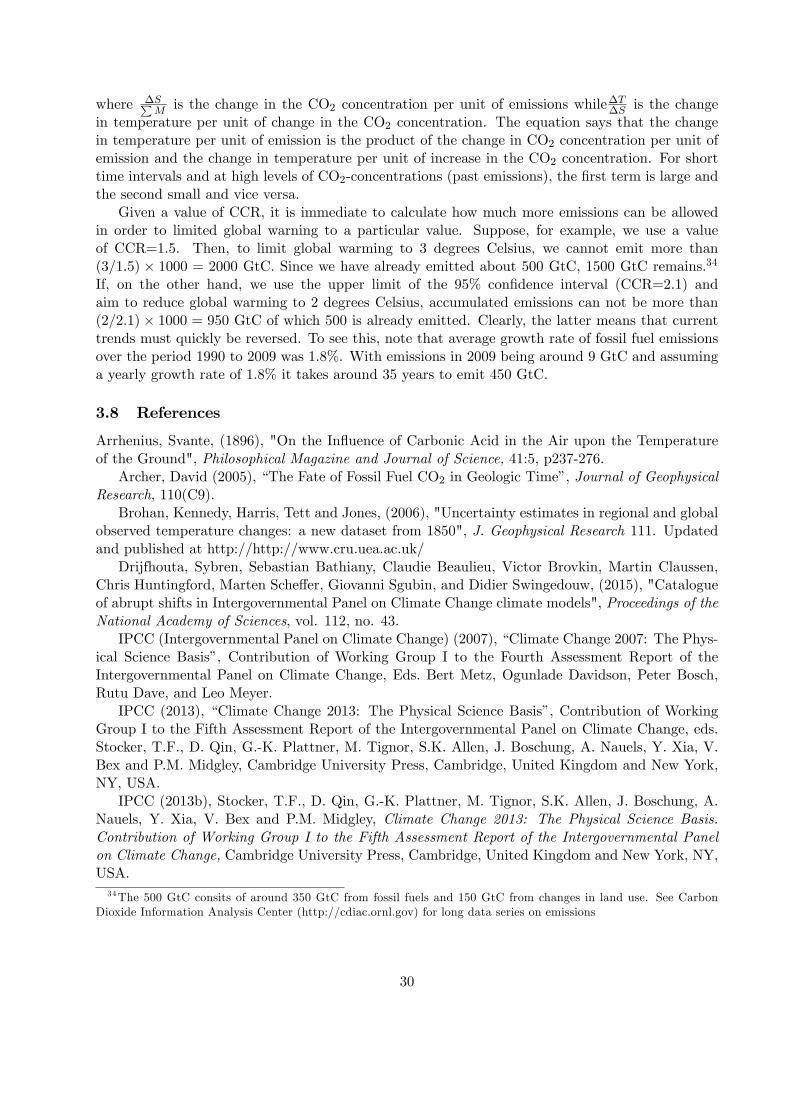
where ∆S∑M is the change in the CO2 concentration per unit of emissions while∆T

∆S is the changein temperature per unit of change in the CO2 concentration. The equation says that the changein temperature per unit of emission is the product of the change in CO2 concentration per unit ofemission and the change in temperature per unit of increase in the CO2 concentration. For shorttime intervals and at high levels of CO2-concentrations (past emissions), the first term is large andthe second small and vice versa.

Given a value of CCR, it is immediate to calculate how much more emissions can be allowedin order to limited global warning to a particular value. Suppose, for example, we use a valueof CCR=1.5. Then, to limit global warming to 3 degrees Celsius, we cannot emit more than(3/1.5) × 1000 = 2000 GtC. Since we have already emitted about 500 GtC, 1500 GtC remains.34

If, on the other hand, we use the upper limit of the 95% confidence interval (CCR=2.1) andaim to reduce global warming to 2 degrees Celsius, accumulated emissions can not be more than(2/2.1)× 1000 = 950 GtC of which 500 is already emitted. Clearly, the latter means that currenttrends must quickly be reversed. To see this, note that average growth rate of fossil fuel emissionsover the period 1990 to 2009 was 1.8%. With emissions in 2009 being around 9 GtC and assuminga yearly growth rate of 1.8% it takes around 35 years to emit 450 GtC.

3.8 References

Arrhenius, Svante, (1896), "On the Influence of Carbonic Acid in the Air upon the Temperatureof the Ground", Philosophical Magazine and Journal of Science, 41:5, p237-276.

Archer, David (2005), “The Fate of Fossil Fuel CO2 in Geologic Time”, Journal of GeophysicalResearch, 110(C9).

Brohan, Kennedy, Harris, Tett and Jones, (2006), "Uncertainty estimates in regional and globalobserved temperature changes: a new dataset from 1850", J. Geophysical Research 111. Updatedand published at http://http://www.cru.uea.ac.uk/

Drijfhouta, Sybren, Sebastian Bathiany, Claudie Beaulieu, Victor Brovkin, Martin Claussen,Chris Huntingford, Marten Scheffer, Giovanni Sgubin, and Didier Swingedouw, (2015), "Catalogueof abrupt shifts in Intergovernmental Panel on Climate Change climate models", Proceedings of theNational Academy of Sciences, vol. 112, no. 43.

IPCC (Intergovernmental Panel on Climate Change) (2007), “Climate Change 2007: The Phys-ical Science Basis”, Contribution of Working Group I to the Fourth Assessment Report of theIntergovernmental Panel on Climate Change, Eds. Bert Metz, Ogunlade Davidson, Peter Bosch,Rutu Dave, and Leo Meyer.

IPCC (2013), “Climate Change 2013: The Physical Science Basis”, Contribution of WorkingGroup I to the Fifth Assessment Report of the Intergovernmental Panel on Climate Change, eds.Stocker, T.F., D. Qin, G.-K. Plattner, M. Tignor, S.K. Allen, J. Boschung, A. Nauels, Y. Xia, V.Bex and P.M. Midgley, Cambridge University Press, Cambridge, United Kingdom and New York,NY, USA.

IPCC (2013b), Stocker, T.F., D. Qin, G.-K. Plattner, M. Tignor, S.K. Allen, J. Boschung, A.Nauels, Y. Xia, V. Bex and P.M. Midgley, Climate Change 2013: The Physical Science Basis.Contribution of Working Group I to the Fifth Assessment Report of the Intergovernmental Panelon Climate Change, Cambridge University Press, Cambridge, United Kingdom and New York, NY,USA.34The 500 GtC consits of around 350 GtC from fossil fuels and 150 GtC from changes in land use. See Carbon

Dioxide Information Analysis Center (http://cdiac.ornl.gov) for long data series on emissions

30

Jones and Mann, (2004), "Climate over past millennia", REVIEWS OF GEOPHYSICS, VOL.42.

Lenton, Timothy M., Hermann Held, Elmar Kriegler, Jim W. Hall, Wolfgang Lucht, StefanRahmstorf and Hans Joachim Schnellnhuber, (2008), ”Tipping elements in the Earth’s climatesystem”, Proceedings of the National Academy of Sciences, vol. 105, no. 6, pages 1786-1793.

Levitan, Dave (2013), ”Quick-Change Planet: Do Global Climate Tipping Points Exist?”, Sci-entific American 25, March 2013.

Matthews, H. Damon, Nathan P. Gillet, Peter A. Stott and Kirsten Zickfeld (2009), "Theproportionality of global warming to cumulative carbon emissions", Nature, Vol 459 June, p829-33.

Nordhaus, William and Joseph Boyer (2000),Warming the World: Economic Modeling of GlobalWarming, MIT Press, Cambridge, MA.

Otto, A, Otto, FEL, Allen, MR, Boucher, O, Church, J, Hegerl, G, Forster, PM, Gillett, NP,Gregory, J, Johnson, GC, Knutti, R, Lohmann, U, Lewis, N, Marotzke, J, Stevens, B, Myhre, Gand Shindell, D, (2013), "Energy budget constraints on climate response", Nature Geoscience, 6(6). 415 - 416.

Schwartz, Stephen, Robert Charlson, Ralph Kahn, John Ogren, and Henning Rodhe (2010),“Why Hasn’t Earth Warmed as Much as Expected?", Journal of Climate, 23

Schwartz, S. E., R. J. Charlson, R. Kahn, and H. Rodhe (2014), "Earth’s Climate Sensitivity:Apparent Inconsistencies in Recent Assessments", Earth’s Future, 2

Rogner, H.-H. (1997), “An Assessment of World Hydrocarbon Resources", Annual Review ofEnergy and the Environment, 22, 217-262.

31

4 Public economics

More than a decade ago, most countries joined an international treaty —the United Nations Frame-work Convention on Climate Change (UNFCCC) —with the ambition of beginning to consider howglobal warming can be reduced and how to cope with whatever temperature increases that areinevitable. More recently, a number of nations approved an additional treaty: the Kyoto Protocolwhich is an international and legally binding agreement that aims at reducing greenhouse gases.

These international collaborations raise several questions. First, why are they necessary in thefirst place? Are the markets not able to allocate the resources in an effi cient way? Why cannoteach individual country just do what is best by itself? In addition, if policy is necessary, then whatexactly does this policy look like?

In order to analyze these questions and/or evaluate the welfare implications of different policies,we first need a crash course in consumer theory, i.e., we first need to assume something about howconsumers value different alternatives. Second, we need to understand that global warming is adifferent type of “good” than a private good like, for instance, a computer that is traded on amarket. We start with consumer theory and consumer preferences.

4.1 Consumer theory

Preferences are the building block of consumer choice. A good way of beginning is to think aboutpreferences in terms of comparisons between different market baskets. A market basket is simplya collection of one or more commodities. It might, for example, consist of various forms of foodand clothing that a consumer buys on a regular basis. The consumer is assumed to be able torank how one basket is preferred to another basket. In fact, if we assume that the preferencessatisfy a number of assumptions —called axioms —we can represent the consumer’s preferences bya mathematical function, a so-called utility function. First we need to define the notation. Supposethat x and y are two market bundles. Then, we will use the following notation

x % y is x is at least as good as yx � y is x is preferred to y

x ∼ y is x is indifferent to y.

The theory of consumer behavior then begins with four axioms for consumer preferences forone market basket versus another.

1. Preferences are complete, which means that a consumer can compare and rank any and allbundles. Specifically, if x and y are two distinct bundles then either x % y or y % x must betrue.

2. Preferences are reflexive. This means that x ∼ x must be true. This is an axiom that mightseem obvious but it is necessary for rational behavior.

3. Preferences are transitive, which means that if x � y and y � z, it must be true that x � z.

4. Preferences are continuous so that if x is preferred to y then bundles “suffi ciently close”to xmust also be preferred to y. This last axiom is often made to rule out certain discontinuousbehavior.

If a consumer’s preferences over bundles satisfy the four axioms, there exists a continuous utilityfunction such that if x � y then u(x) > u(y). The utility function is then a way of describing the

32

choices that the consumer makes. Potentially, the utility function will contain all “goods” thatthe consumers value and care about. Hence, the arguments in the function do not only have tobe market goods, but could, for instance, equally well be clean air, biodiversity and other people’swell being and their consumption. In most cases, however, economists abstract from most of thesearguments in unless they are perceived to be necessary for the analysis.

With the utility function we can then evaluate how a consumer will react to an imposed tax onthe consumption bundle she consumes. In addition, by comparing the utility she gets from the twobundles (with and without the tax) we can evaluate how her welfare is affected. However, beforeanswering the questions about why policy might be needed on issues related to climate change, weneed to know for what goods markets can be expected to work effi ciently. This is the topic of thenext section.

4.2 The first theorem of welfare economics

Consider an economy with two consumers: consumers 1 and 2 that can both be completely describedby their preferences, �1 and �2, and their initial endowments of the two commodities, ω1

1, ω21, ω

12

and ω22, where subscripts denote the agent and superscripts denote the goods. The concept of a

good is very broadly defined and goods are distinguished by time, location and states of the world.These consumers are allowed to trade the goods among them to become better off and there isassumed to exist a market for each good. The agents are assumed to behave competitively, i.e.,they take prices as given. An allocation is a collection of consumption bundles that describes whateach of the two agents is holding. The prices p1, p2, are endogenously determined in the tradingprocess.

In this economy, each agent i = 1, 2 is solving the following problem

maxx1i ,x

2i

u(x1i , x

2i

)s.t.

p1x1i + p2x

2i = p1ω

1i + p2ω

2i .

The outcome of this individual problem is the consumer’s demand function. Formally, letx1

1 (p1, p2) be agent 1’s demand function for good 1 and x12 (p1, p2) be agent 2’s demand function

for good 1, and define the analogous expressions for good 2.What are the features of the equilibrium outcome resulting from such a process? What is the

optimal outcome? Which allocative mechanisms can be used to achieve the optimal outcome? Toanswer these questions, we will use the concept of a Walrasian equilibrium. An allocation is aWalrasian equilibrium if

x11 (p∗1, p

∗2) + x1

2 (p∗1, p∗2) = ω1

1 + ω12,

and

x21 (p∗1, p

∗2) + x2

2 (p∗1, p∗2) = ω2

1 + ω22,

Hence, in words, a Walrasian equilibrium is an allocation where aggregate demand (here con-sisting of the sum of the two consumers’demand) for each good is exactly equal to the supply ofthe good. Or, put differently, an allocation where all markets clear. A Walrasian equilibrium canbe shown to exist.

Theorem 1 First theorem of welfare economics. If the allocation is a Walrasian equilibrium, thenit is also Pareto effi cient.

33

Proof. Assume that the equilibrium is not effi cient, i.e., that there is some other feasible allocation(y1

1, y12, y

21, y

22

)such that

y11 + y1

2 = ω11 + ω1

2 (15)

andy2

1 + y22 = ω2

1 + ω22, (16)

and (y1

1, y21

)%1

(x1

1, x21

)(17)

(y1

2, y22

)%2

(x1

2, x22

), (18)

where at least one of the comparisons in (17) and (18) is strict so that one agent strictly prefersthe

(y1, y2

)-bundle. Assume now that it is agent 1 who strictly prefers the y-bundle so that the

comparison in (17) is strict. The two equations (15)-(16) then say that the y-allocation is feasibleand the next two that it is strictly preferred by agent 1 and weakly preferred by agent 2 to thex-allocation. But the hypothesis is that we have a market equilibrium where each agent purchasesthe best bundle she can afford. If

(y1

1, y21

)is better than the bundle agent 1 is choosing, it must

be that it costs more than agent 1 can afford since by assumption it is preferred and affordable.Similarly, if agent 2 is indifferent between

(x1

2, x22

)and

(y1

2, y22

), it must be that the bundle

(y1

2, y22

)costs at least at much as the

(x1

2, x22

), otherwise agent 2 would not be indifferent between the two

bundles. From axiom 4 above, the agent could then have spent more on any of the two goods whichwould have increased the utility. Hence, we have

p1y11 + p2y

21 > p1ω

11 + p2ω

21

p1y12 + p2y

22 ≥ p1ω

12 + p2ω

22.

Now add these two equations to get

p1

(y1

1 + y12

)+ p2

(y2

1 + y22

)> p1

(ω1

2 + ω11

)+ p2

(ω2

2 + ω21

).

Finally, substitute equation (15)-(16) into the above equation to get

p1

(ω1

1 + ω12

)+ p2

(ω2

1 + ω22

)> p1

(ω1

2 + ω11

)+ p2

(ω2

2 + ω21

),

which is clearly a contradiction, since the left-hand side and the right-hand side are the same.The theorem states that if the assumptions are satisfied, the market equilibrium is Pareto

effi cient, which means that it is not possible to make all agents better off. In other words, it is notpossible for policy to increase the effi ciency in the economy. Here, we have a simple endowmenteconomy with only two agents and two goods, but the theorem generalizes to an arbitrary number ofagents and goods. In addition, recall that goods are very broadly defined and can be distinguishedby time (i.e., different time periods), location and states of the world (i.e., when consumption ofthe goods is subject to uncertainty). It also applies to economies with firms and production of thegoods. The theorem is thus very strong.

However, the outcome completely depends on the initial distribution of endowments and there-fore it need not be considered as "fair". Thus, there could be room for a policy to change thedistribution of resources.

This brings us back to the question raised at the beginning of the chapter: are the markets ableto allocate the resources in an effi cient way when it comes to global warming (when abstracting

34

from redistributional issues)? Can we apply the first theorem of welfare economics and just trustthat when firms, consumers and countries trade, this will result in a Pareto effi cient outcome? Theanswer is no and the reason is that one of the important assumptions that are required for thetheorem to be true is not fulfilled. We now turn to study the effects of market failure, i.e., whensome of the assumptions of the welfare theorem do not hold and hence, we can no longer rely onmarket equilibria to get Pareto optimal outcomes.

4.3 Externalities

There are many cases where the actions of an individual or a firm directly affect other individualsor firms, where one firm imposes a cost on other firms but does not compensate the other firm or,alternatively, where one firm receives benefits from other firms but does not pay for the benefit.Instances where one individual’s actions impose a cost on others are called negative externalities andinstances where one individual’s actions yield a benefit on others are called positive externalities.Externalities are labeled consumer externalities or producer externalities depending on the sourceof the externality. Highway congestion is an example of a consumer externality and industrialpollution is an example of a producer externality. In the presence of externalities, the first theoremof welfare economics does not hold because there are things that people care about that are notpriced. Specifically, the assumption that there is a market for every good is not true. In the case ofa negative externality, more of the product is produced and sold than the effi cient amount. Sincethe marginal benefit is not equal to the marginal cost, a deadweight welfare loss arises.

4.3.1 An example with a consumer externality

Consider now once more the example in the first section and assume that the utility functionfor agent 2 is the same as before, while the utility function of agent 1 also depends on agent 2’sconsumption of good 1, i.e.,

u1

(x1

1, x21, x

12

)and

u2

(x1

2, x22

).

Examples could, for instance, be tobacco smoke or alcohol. Now, it no longer needs to be truethat

p1y11 + p2y

21 > p1ω

11 + p2ω

21.

In fact, the y-allocation may be affordable and preferred if it has a y12 that is significantly

different and better for agent 1 than x12. Both agents are still choosing allocations that are best for

them but their choices no longer reflect the social benefits. In this case, agent 1 cares about theconsumption of agent 2 but cannot affect this choice and agent 2 ignores it. In other words, thereare things that the agents care about that are not priced.

4.3.2 An example with a production externality

Consider an economy with two firms labeled 1 and 2. Firm 1 produces an output X which is soldon a competitive market. However, the production of also imposes a cost γ (X) on firm 2. Wemay consider this as a technology used by firm 1, i.e. for each unit of output X it produces it alsoproduces X units of pollution which harm firm 2. We call γ (X) an externality since it is externalfrom the point of view of the agent who controls X.

35

If we denote the price of output by p, the profits of the two firms are

π1 = maxX

pX − c (X)

π2 = −γ (X) .

Both cost functions are assumed to be increasing and convex. For simplicity, additional profitsthat firm 2 might have are, for simplicity, abstracted from.

The equilibrium amount of output in this economy is

p = c′ (X) .

However, this amount is too large from a social point of view. The reason is that firm 1 onlytakes the private costs into account, while ignoring the social costs which are the private costs plusthe costs imposed on the other firm.

So what is the effi cient amount of output in this economy? To find this out, we set up the socialplanner’s problem. This implies maximizing profits while taking all costs into account. Formally:

π = maxX

pX − c (X)− γ (X) .

Note that this is the same problem as the problem of a merged firm. The first-order conditionis

p = c′ (X) + γ′ (X) (19)

which is evaluated at the optimal value of X.The output that satisfies equation (19) is the effi cient amount of output. It is characterized by

that price being equal to the social cost, being equal to the sum of the marginal private cost andthe marginal externality. By internalizing the externality, the ineffi ciency is taken care of.

4.4 An example with CO2 emissions

Here, we consider the example with a production externality and also discuss different solutionsto that problem. The setting is one where a representative firm uses an input like fossil fuel toproduce an output. The use of fossil fuels is bad since it produces CO2-emissions which have anegative effect on the climate. The result is an increased frequency of weather shocks such as heatwaves, droughts, flooding etc. These costs can be measured as a share of final output (GDP). Here,we abstract from the exact mechanism through which the input affects the climate and just assumethat the use of fossil fuels reduces GDP (we will explicitly add the climate later). Since agents arenot facing the full costs of their actions, they use too much fossil fuel.

We start out without externalities to get an understanding of the model and to see what featuresthe equilibrium has without externalities. There are two sectors in the economy: one that producesfossil fuels E, and one that produces final output Y . Both firms in these sectors are assumed tobehave competitively. Moreover, the resources required to produce one additional unit of fossilfuels µ, is assumed to be constant (and denoted in terms of final output). This last assumptionis not based on any estimated features of reality but is made purely for simplicity. In reality, itcould very well be the case that it is more and more costly to extract additional units of fossil fuel(implying a convex cost function).

36

4.4.1 Case 1: no externality

Suppose there is a perfect market where suppliers of fossil fuel supply fossil fuel E that they canproduce at marginal cost µ.35 The assumption of perfect competition implies that

p = µ,

i.e., the price equals the marginal cost.The representative firm in the final goods sector uses fossil fuels and labor as inputs for producing

an output y. Specifically, the production function for output is given by

Y ≡ f (E,L) = EνL1−ν , (20)

with 0 < ν < 1, 0 < µ < 1 and ν > µ. Finally, the total supply of labor is fixed at one unit, i.e.,L = 1.

Using the fact that p = µ, the profit maximization problem for the firm is

π = maxE

EνL1−ν − µE − wL.

The first-order condition with respect to E and L is respectively given by

νEν−1L1−ν = µ (21)

and

(1− ν)EνL−ν = w.

Now use L = 1 in (21) giving

E =(µν

) 1ν−1

,

or

E =

(ν

µ

) 11−ν

. (22)

Final output is then given by

Y =

((ν

µ

) 11−ν)ν,

which can be written as

Y =

(ν

µ

) ν1−ν

. (23)

35We now disregard the possibility that the total supply is finite. We will return to this in later chapters.

37

4.4.2 Case 2: adding an externality

Let us now assume that the use of fossil fuels causes costs in the sense that it reduces final output.The representative firm does not take the negative effect on production into account when decidinghow much fossil fuel to use. We maintain perfect markets, requiring that we have a large numberof identical firms. From the individual firm’s perspective, the average level of fossil energy use inthe economy, denoted by E, that has a negative effect on production is exogenously given, i.e., theindividual firm cannot do anything about it.

The production function for final output is then given by

Y ≡ f(E,E,L

)= E

−γEνL1−ν ,

with γ > 0 and where the term E−γcaptures the damages caused by the use of fossil fuels. Hence,

final output is decreasing in E. In equilibrium, it must be true that E = E since all firms are thesame, but the important thing is that the representative firm does not view E as a choice variable.We also assume that ν > γ so that when E increases, and consequently E increases by the sameamount, output also increases.

Since nothing has changed in the sector producing fossil fuels, we still have that p = µ. Theprofit maximization problem for the firm is then

π = maxE

E−γEνL1−ν − µE − wL.

The first-order condition with respect to E and L is, respectively, given by

νE−γEν−1L1−ν = µ, (24)

and

(1− ν)E−γEνL−ν = w. (25)

Once more, using the facts that L = 1, and that in equilibrium E = E in (24), we get

νEν−γ−1 = µ,

which can be solved for E:

Elf =

(ν

µ

) 11+γ−ν

, (26)

where the index lf denotes the outcome in laissez faire (as opposed to the amount of E (denotedEsp) in the social planning problem below). Final output is given by

Y =

((ν

µ

) 11−ν+γ

)ν−γL1−ν ,

or, since L = 1,

Ylf =

(ν

µ

) ν−γ1+γ−ν

. (27)

The level of output is lower than without the externality. This is expected since the externalityis causing losses. In addition, when the cost of the externality goes to zero, Ylf approaches the

38

quantity produced in the case without the externality (see equation 23). Now, multiply both sidesof (24) by E and note that

νE−γEνL1−ν︸ ︷︷ ︸Y

= µE.

Similarly, multiply both sides of (25) by L to get

(1− ν)E−γEνL1−ν︸ ︷︷ ︸Y

= wL.

The total profit is thenπ = Y − νY︸︷︷︸

µE

− (1− ν)Y︸ ︷︷ ︸wL

= 0−

4.4.3 The social planning problem

The social planning problem can be considered as an answer to the question of what the optimalthing is to do. We imagine that there is a benevolent planner that is maximizing profits whiletaking all costs into consideration. Hence, the planner does not take E as given, but realizes thatE = E. Assuming that the marginal value of output equals the price of output, the maximizationproblem is

maxE

E−γEνL1−ν − µE. (28)

This can be written as

maxE

Eν−γL1−ν − µE. (29)

The first-order condition with respect to E is

(ν − γ)Eν−γ−1L1−ν = µ. (30)

Using the fact that L = 1, the above equation can be solved for E:

Esp =

(ν − γµ

) 11+γ−ν

< Elf =

(ν

µ

) 11+γ−ν

.

Production is then finally given by

Ysp =

((ν − γµ

) 11+γ−ν

)ν−γ,

or

Ysp =

(ν − γµ

) ν−γ1+γ−ν

.

Note once more that we can multiply both sides of (30) by E to obtain

(ν − γ)Eν−γL1−ν︸ ︷︷ ︸Ysp

= µE. (31)

39

In equilibrium, the value of production is strictly larger than the costs. Combining (29) and(31), we get

Ysp − (ν − γ)Ys︸ ︷︷ ︸µE

,

or

Ysp (1− (ν − γ)) > 0, (32)

As can be seen in the figure, total production (the solid blue line) minus the costs employed(the red dashed line) is maximized when the distance between the two curves is the largest. Thisoccurs at Esp = 1 in the figure while the market solution is above 2. 36 For E > 1,additional unitsof fossil fuel increase the production but the marginal increase in production is then less than themarginal cost and this is ineffi cient.

4.5 Solutions

It has now been illustrated that when firms are faced with a negative externality, optimal output islower than without an externality. This implies that the use of fossil fuel is lower in the centralizedfirst best solution than in the decentralized solution. The question is then if it is possible toimplement some policy that ensures that the first best allocation is achieved also in the decentralizedeconomy. In this section, we will discuss different solutions to the problem, including assigningproperty rights, taxes and quantity restrictions.

4.5.1 Property rights

One way of viewing the problem is to say that the property rights are not well defined. In particular,the Coase theorem (after Ronald Coase) states that if trade in an externality is possible and thereare no transaction costs, bargaining will lead to an effi cient outcome. This is regardless of theinitial allocation of property rights. However, in the setting described here, the bargaining processis unlikely to be effi cient. If the right to pollute the atmosphere is given to an individual (or a groupof individuals), this individual effectively controls fossil fuel use. This agent is then a monopolistand cannot be expected to behave in a way that is socially optimal. Second, it is not realisticto give some agent the property rights to the air and the atmosphere. The Coase theorem is thusof less use when it comes to externalities related to climate change, since the solutions suggestedabove do not realistically apply in a global setting. A related problem is that the atmosphere reallyis a public good (it is hard to exclude people from using it). The problems of pricing the externalitythen also have all the characteristics that are associated with the pricing of public goods.

4.5.2 Merging

According to the First Welfare Theorem, whenever a market allocation is not Pareto effi cient, thenthere is some way of increasing the aggregate surplus. As noted above (in section 4.3.2), if theexternality of one firm has a negative effect on the profits of another firm, it will always be effi cientfor the firms to merge. In other words, by coordinating the actions of both firms, more profits canbe generated than when the firms act separately. If the representative firm was just one firm, thenit would internalize the costs on production from using fossil fuel since it would then bear the fullcost from fossil fuel use. This firm would then set Elf = Esp (convince yourself of this!). However,

36The parameters in the example in the figure are set to α = 0.8, β = 0.2 and φ = 0.6.

40

in a global setting it is not realistic or desirable that all firms that are using fossil fuel merge. Inaddition, even if they would do so, there would be other problems since that firm then could notbe expected to behave competitively. Another, more promising solution is to use taxes.

4.5.3 Pigouvian taxes

As shown in section 2, in the presence of negative externalities, the social cost of a market activityis not covered by the private cost of the activity. The market outcome is then not effi cient and itmay result in over-consumption of the good. One solution to this problem is to impose a so-calledPigouvian tax on the activity that generates negative externalities. The tax should then be set sothat it exactly reflects the size of the negative externality. In this way, the corrective tax increasesthe price so that it includes both the private and the social cost.

A tax on fossil fuel carbon tax can enhance effi ciency if it corrects the market distortions thatarise when people do not take the external effects of their energy consumption into account. Toimplement the first best in the decentralized economy, the planner can impose a proportional taxon the use of energy. The profit maximization problem is then

π = maxE

E−γEνL1−ν − (µ+ τ)E − wL,

where τ is the Pigouvian tax. The first-order conditions with respect to E and L are then, respec-tively, given by

νE−γEν−1L1−ν − τ = µ (33)

and

(1− ν)E−γEνL−ν = w. (34)

From (30), it follows that the social planner should set

τ = γE−γEν−1L1−ν , (35)

since this implies that

(ν − γ)E−γEν−1L1−ν = µ,

which in equilibrium, i.e., with E = E, gives the same condition as in the first best:

E =

(ν − γµ

) 11+γ−ν

.

Plugging in the expression for Esp into (35), we get that the tax is given by

τ =γµ

ν − γ . (36)

Note that an effective result requires that all nations agree on implementing the optimal tax.However, if they do, an individual country has incentives to deviate and increase E, becauseprofits are positive at the optimal allocation (see equation 32). Hence, in a competitive settingthe government has incentives to try to undercut other governments by offering lower tax rates toincrease production and/or to attract firms to its country. Note that this incentive is true for all

41

countries. Unless the tax can be combined with other international sticks and/or carrots, outputis likely to increase and return to the ineffi cient market allocation (equation 22).

Another practical problem is that for the tax authorities to derive the effi cient tax rate, theymust actually know the externality cost function. However, a key problem is that in many cases, theauthorities do not have this information. In fact, Pigou himself wrote that "It must be confessed,however, that we seldom know enough to decide in what fields and to what extent the State, onaccount of [the gaps between private and public costs] could interfere with individual choice".37

This is particularly true when it comes to issues of climate change. First, there is a really largeuncertainty about how much the temperature can be expected to increase and second, what damagesdifferent temperatures will cause.

4.5.4 Quantity restrictions

If the tax authorities actually know the externality cost function, they can simply just directly tellthe firms how much to produce. That is, another option for the government is to directly restrictthe quantity. A variant of quantity regulation of emissions is the cap-and-trade system, whichinvolves tradable emissions permits. A number of emission licenses for a specified pollutant arethen issued. If someone wants to emit more than what it is licensed for, it may buy additionallicenses from other owners of licenses. Conversely, a firm that has more licenses than it intends touse can sell its surplus. The advantage of allowing trade is that some firms can reduce emissionsmore cheaply than others. For a firm with high costs of reducing emissions, it is more effi cient tobuy permits from firms that are able to reduce emissions more cheaply. This gives everyone anincentive to reduce pollution.

4.5.5 Taxes vs quantities

As shown above, the regulator can control pollution either by regulating the price, i.e., by imposinga Pigouvian tax or by directly setting emission quantities. In the absence of uncertainty, thesetwo policy instruments are completely equivalent. Hence, with complete knowledge and perfectinformation about the costs of reducing the pollution and the benefits of cleaner air, there is a formalidentity between the use of prices and quantities as planning instruments. However, in the presenceof uncertainty this may no longer be the case. In reality, there is likely to be some uncertaintyabout both the exact specification of the cost function and the benefit function. The question iswhich of the two instruments that is then preferred? This problem is studied by Weitzman (1974).Specifically, he considers the case where an amount q of a certain good can be produced at acost C(q), yielding benefits B(q). However, the costs also depend on a disturbance term (i.e., arandom variable): C(q, µ). Similarly, the benefits also depend on another random variable: B(q, η).Weitzman suggests that we could consider q as the cleanliness of air being emitted by a certaintype of source. The costs then depend on q but they may be uncertain because the technologyquantified by µ is uncertain. At a given level of q, the benefits may also be uncertain since they,among other things, depend on the weather, measured by η.

Specifically, he finds that price instruments are favoured when the marginal benefit schedule isrelatively flat and quantity instruments are favoured when the marginal cost schedule is relativelyflat. Price controls are preferred in the former case because if the social marginal benefit is approx-imately constant in some range, the best policy is to set the price and let the producers find theoptimal output themselves (after eliminating the uncertainty from costs). This result in the latter

37Pigou (1954).

42

case comes from the fact that when marginal costs are nearly flat, the smallest miscalculation orchange results in either much more or much less than the desired quantity.

Despite the close resemblance between the two systems in theory, they are somewhat differentin practice. Specifically, they produce different types of uncertainty. When the regulator chooses touse taxes, the price is clear for the polluters, but the amount of pollution generated is not. Whenrestricting quantity, the government is aware of the amount of pollution, but the price of emissionswill not be clear.

There is an ongoing debate about whether price or quantity restrictions are the better. Nordhausargues in favor of the carbon tax by stating that quantitative limits may produce volatility in themarket price of carbon.38 This arises because of the inelasticity of both supply and demand ofpermits. The volatility might be economically costly for firms and provides inconsistent signals toprivate-sector decision makers. A carbon tax, on the other hand would, according to Nordhaus,provide consistent signals and would not vary so severely. He also thinks that the tax approachprovides less opportunity for corruption than do quantitative limits, because the tax approachdoes not create artificial scarcities and thus encourages rent-seeking behavior. All in all, Nordhausadvocates the conceptual simplicity of the tax approach and views the cap-and-trade approachembodied in the Kyoto model as a poor choice of mechanism.

However, the tax-based approach also has shortcomings. First of all, even though taxes area well-used tool in general, it is on unfamiliar ground in international environmental agreements.Moreover, there are some concerns regarding the price elasticity on carbon: how well do carbonemissions respond to increased prices?

In addition, since taxes cannot guarantee a specific emission level, a quantity restriction may bedesirable because it better allows the regulator to ensure a specific level of emissions, which makesthe system more predictable regarding climate change. However, knowing the correct quantity levelof emissions that will not cause excessive climate change is challenging or even impossible seeingthat we do not have suffi cient knowledge of all the direct and indirect effects on the climate, aswell as the carbon system or the economic costs of climate change. Moreover, while a tax generatescosts on the firms as well as revenue for the government, cap and trade often involve handing outlicenses to existing agents, so that the revenue goes to the industry instead of the government.This might make quantity regulations more feasible politically speaking, since the firms are partlycompensated for their loss. Hence, according to Krugman, it will probably be more challenging toachieve agreements in national parliaments regarding taxes, considering the powerful interests oflobbying energy-intensive firms affected by the regulation.39 Even though a market-based policyinstrument is a necessary condition for giving disincentives on carbon emissions, Krugman stilladvocates supplementing them with a direct regulation (legislation) on coal use.

4.6 Carbon Leakage

Since it is diffi cult to agree on an international policy, some countries might just decide to startreducing emissions by themselves. In this way, they will “move first” and then hope that otherswill follow. What is the consequence of this policy? Is it good for the environment or will it justhurt the countries that implement the policy with no effects on global aggregate emissions? Onepotential problem is carbon leakage, i.e., the fact that if one country imposes a tax on carbon, thismight just shift the use of carbon to another country (that has a less strict climate policy). Below,we consider two cases to illustrate some determinants of whether carbon leakage is likely to occur.

38Nordhaus (2009).39Krugman’s article in the New York Times, April 5, 2010.

43

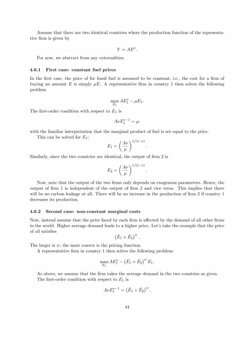
Assume that there are two identical countries where the production function of the representa-tive firm is given by

Y = AEν .

For now, we abstract from any externalities.

4.6.1 First case: constant fuel prices

In the first case, the price of for fossil fuel is assumed to be constant, i.e., the cost for a firm ofbuying an amount E is simply µE. A representative firm in country 1 then solves the followingproblem

maxE1

AEν1 − µE1.

The first-order condition with respect to E1 is

AνEν−11 = µ.

with the familiar interpretation that the marginal product of fuel is set equal to the price.This can be solved for E1:

E1 =

(Aν

µ

)1/(1−ν)

.

Similarly, since the two countries are identical, the output of firm 2 is

E2 =

(Aν

µ

)1/(1−ν)

.

Now, note that the output of the two firms only depends on exogenous parameters. Hence, theoutput of firm 1 is independent of the output of firm 2 and vice versa. This implies that therewill be no carbon leakage at all. There will be no increase in the production of firm 2 if country 1decreases its production.

4.6.2 Second case: non-constant marginal costs

Now, instead assume that the price faced by each firm is affected by the demand of all other firmsin the world. Higher average demand leads to a higher price. Let’s take the example that the priceof oil satisfies (

E1 + E2

)ψ .The larger is ψ, the more convex is the pricing function.

A representative firm in country 1 then solves the following problem:

maxE1

AEν1 −(E1 + E2

)ψE1.

As above, we assume that the firm takes the average demand in the two countries as given.The first-order condition with respect to E1 is

AνEν−11 =

(E1 + E2

)ψ .44

0

1

2

3

4

5

0.2 0.4 0.6 0.8 1x

Figure 13: Supply and demand, country 1, ψ = 10

In equilibrium, all firms are doing the same so if we focus on country 1, we have

AνEν−11 =

(E1 + E2

)ψLet us now in figure 13 plot the LHS and the RHS against E1. Furthermore, we plot the RHS

for two values of foreign average demand E2, one high and one low. We first do this for a highvalue of ψ, namely 10.40The downward-sloping curve is AνEν−1

1 , the marginal product of fossil fuelin country 1. The leftmost upward-sloping function is the price as a function of domestic demandgiven high foreign demand and the rightmost curve is price given low demand. As we see, the lattercurve is the same as the former, but shifted to the right by the amount E2 has fallen. In fact we,see leakage in this case is almost complete.

Let’s now in figure 14 do the same experiment but instead set ψ = 1. In this case, the price ismuch less sensitive to aggregate global demand. Despite the fact that we change foreign demandby the same amount as in the previous figure, domestic demand changes much less. In other word,leakage is much smaller.

4.7 Problems with implementing the policy

4.7.1 Universal participation

As is clear from the above, it can be highly problematic to implement the effi cient policy in practice.Even though all countries in our examples were identical, it was problematic because each of themhad an incentive to deviate from the effi cient tax rate. In reality, there are many more features thatadd to the diffi culties because countries are heterogeneous. For this reason, they might disagree onhow the policy should be divided between different countries.

Countries may also have different incentives to reduce emission because of different perceptionsof damages, income levels, political structures, environmental attitudes and country sizes. Russia40We use the parameters A = 1, α = 0.3, and E2 = 0.2, 0.4, respectively.

45

0

1

2

3

4

5

0.2 0.4 0.6 0.8 1x

Figure 14: Supply and demand, country 1, ψ = 1

could, for instance, argue that it might be less affected by a temperature increase. A poor countrymay advocate that it had not yet contributed to much of the damage as well as point out that itslow income level makes it challenging to contribute.

For an outcome to be self-enforcing, it must be viewed as being fair to all parties. There areways of deterring incentives to non-participation when the issues regard unfairness. One alternativeis side payments– i.e. countries that gain most from an agreement compensate those who wouldlose or gain least – which can implicitly be provided through the international tradable permitsystem. In general, market-based instruments can be considered as providing positive incentives inthe sense that they can reduce costs overall and potentially for all parties.

Still, these positive incentives might not be suffi cient to overcome the severe free-riding prob-lems. Hence, negative incentives such as punishment for non-participation might also be necessary.However, ensuring that such incentives provide credible threats is diffi cult given the lack of a pow-erful world government with coercive powers.

4.8 References

Dell, M., Benjamin F. Jones and Benjamin A. Olken. "Climate change and economic growth:evidence from the last half century", NBER Working Paper No.14132.

Krugman, P., "Building a Green Economy, the New York Times, April 5, 2010.Nordhaus, W., A question of balance, Weighing the options on global warming policies", Yale

University press, New Haven & London, 2008.Nordhaus, W., "Economic issues in designing a global agreement on global warming." Keynote

address prepared for Climate Change: Global Risks, Challenges and Decisions. Copenhagen, 2009.Pigou, A. C., Some Aspects of the Welfare State, 1954.Weitzman M, "Prices vs. quantities", Review of Economic Studies 1974.

46

5 Growth theory in climate research

The relationship between climate and economic growth has been of interest in social research fora considerate amount of time. The subject of growth is relevant for climate research in a numberof ways. First of all the climate is– indirectly, via the carbon cycle– influenced by the burning offossil fuels. Clearly, the use of fossil fuel is linked to economic activity and therefore projections offuture fossil fuel use is interlinked with aspects of economic growth.

Secondly, there are different views on the reversed effect, namely the effect from climate changeon the economy. One perspective is that long-run average temperature affects economic performancenegatively, through a variety of channels, which may have implications on economic decisions onactions against climate change.

Clearly, there are several factors that connect growth and climate economics. Throughout thischapter, however, we will mainly lay our focus on the demand side of the economy as opposed tothe supply side.

5.1 Empirics

There is large variation in per capita income as well as growth rates across countries’economies andgrowth rates do not remain constant over time. The following graphs are in log scales and illustrateboth the distribution of prosperity across countries as well as its evolution over time. The followingfigure shows the development of GDP per capita in a number of countries over close to two hundredyears. As we see, the curves for the US and Britain are fairly close to linear implying the growthrate has been fairly stable during this long time period.41 In some of the other countries, growthis more unstable with stagnant periods and growth "miracles".

The next figure shows the distribution of countries with regard to their GDP per capita in 1960,1980 and 2000. The distribution has shifted to the right over time but there is no clear tendencytowards a wider distribution.

Using population weights, the shift to the right is more pronounced.From the perspective of this book, it is of particular interest that there is a negative correlation

between the average temperature in a country and its GDP per capita. This is illustrated in thefollowing graph, which also shows how climate change has affected the countries so far (rings vscrosses) and the variability of the climate. The graph also shows the large variation in GDP percapita —in the order of 4-5 log points, implying a ratio between the richest and the poorest countryin the order of 50 − 150.42 We will make an attempt to use growth theory to account for thesedifferences below.

5.2 Growth accounting

On a general level output is determined by different factors. One is the availability of factors ofproduction (capital, labor, raw materials) and another is their “effi ciency levels”. Other factorsare the quality of the capital (a broad notion of capital includes infrastructure); the amount ofhuman capital/knowledge embodied in people; as well as how effi ciently the inputs are used. Arethe factors matched in the most productive way?

Under some simplifying assumptions, we can think of output in a country as a function ofcapital and labor

Y = f(K,L)

41The y-axis uses a log scale, implying that a constant growth rate gives a straight line.42e4 ≈ 55, e5 ≈ 148.

47

Figure 15: Historic growth

Figure 16: Distribution of countries according to PPP-adjusted GDP per capita.

48

Figure 17: Distribution of countries according to PPP-adjusted GDP per capita.

where for simplicity we abstract from raw materials, such as fossil fuel. Capital and labor aredenoted factors of production and the relation between output and these factors is described bythe aggregate production function f.

The amount inputs differs between countries due to differences in labor force participation andperhaps more importantly, due to difference in skill and education. By measuring K and L onecan then assess how each of these factors matters.

To decompose differences in output between countries, we may use a method to measure thecontribution of different factors to economic growth. Indirectly we thus compute the rate of tech-nological progress, measured as the “Solow residual”, in an economy. Under the assumptions thatoutputs and inputs can be measured in comparable ways across countries; the existence of an aggre-gate production function that is identical across countries except for a scalar “productivity” level(A) allows us to account for differences in income between countries. We assume output in countryi is given by

Yi = AiKαi l

1−αi ,

If a value of α is assigned to this equation, we may perform a simple accounting exercise tobreak down growth in output into growth in capital, growth in labor and growth in technology,respectively.

Capital/labor share of incomeWe can show that α is capital’s share of output and that labor share of output is 1 − α by

looking at the first-order conditions in the firms maximization problem to obtain expressions for

49

Figure 18: Blue circle (red plus) is mean temp in 1950-1959 (1996-2005). Gray lines is range of annualtemperature over sample period.

50

prices, w and r, as functions of capital stocks;

maxK,L

π = AKαL1−α − rK − wL

Taking the derivatives

∂π

∂K= αAKα−1L1−α = r

∂π

∂L= (1− α)AKαL−α = w

If markets are perfect, firms will make sure that the rental rate of capital r and the wage w isequal to the marginal productivities. Multiplying the two equations above K and L, respectivelyand dividing by Y , gives capital’s share and labor’s share of firm revenues , respectively.

α =rK

Y

1− α =wL

Y

By using this relation, we can directly find the parameter α by measuring the the income shareof capital in GDP. Over time and across countries, it turns out that this number has been quitestable at around 0.3.

Consider two countries i and j, with output Yi and Yj. Using the production function, we have

YiYj

=AiK

αi L

1−αt

AjKαj L

1−αj

Taking natural logs of this ratio yields:

log Yi − log Yj = [logAi − logAj ] + α[logKi − logKj ] + (1− α)[logLi − logLj ] (37)

The second (third) term on the right hand side in the equation is the importance of capital(labor) in explaining output differences between i and j. The first term on the right hand side isa “residual”and "explains" what cannot be accounted for by the other factorsand is said to be ameasure of total factor productivity. Total factor productivity is often referred to as “technology”,but in this case one should keep in mind that it is technology in the widest possible sense. It isserving as a catch-all for anything else that is left unexplained by the other two factors, labor andcapital. Specifically, the residual can be interpreted as the extent to which the assumptions areoff; mismeasurements of inputs and outputs; an inappropriate assumption regarding the aggregatetechnology (e.g., it would look different in an agricultural economy, a manufacturing economy, anda service economy); ineffi ciencies in production which could be caused by poor institutions, poorinfrastructure, etc.; or differences in technology across countries.

5.2.1 Measuring factor inputs

Countries differ a lot regarding how educated their workers are as well as in terms of the marginalvalue of a year of education in terms of productivity. However, we assume that a year of basiceducation is worth the same everywhere. Furthermore, each additional year gives the same “pre-mium”. In the U.S., a multitude of studies indicate that a year of additional education raises a

51

worker’s wage by 6 − 10% and studies in other countries give similar results.43 Lastly, we assumethat there are no externalities to schooling, i.e., all returns to schooling accrue to the individual.Assuming negligible training and education of the workers in the poorest countries and normalizingtheir quality to 1, workers in the richest countries then have 12 years more of schooling than theworkers in the poorest countries. It then follows that Li is 1.0812 ≈ 2.5 and Lj = 1 if consider arich and a poor country of the same size in terms of worked hours.

logLtop − logLbottom ≈ log 2.5 ≈ 0.9.

Multiplying this number by 0.7, we have that the last term on (37) is 0.63 if we use a very richand very poor country.

We will return to how to measure capital inputs later, but as an example, let us use the factthat capital/output ratios tends to be fairly stable along a economic development. Then, if wewant to account for a log difference log(Yi)− log(Yj) of 4 (implying an income ratio of around 50),the contribution from differences in capital stocks is given by 0.3∗4 = 1.2. In sum, we can thereforeaccount for 0.63 + 1.2 = 1.83 of the 4 log point difference, i.e., a bit less than half, by differences inquality adjusted labor and capital.

5.3 The Solow growth model

Solow’s growth model provides an important foundation for understanding growth and has becomethe work-horse model that modern macroeconomic models are built on. In the simple Solow modelwithout technology growth, economies may grow for a while, but not perpetually. It will graduallymove towards its steady state level, which in the simplified model is a point where there is nopermanent economic growth. An economy that starts off with a stock of capital per worker belowits steady state level will experience growth along the transition path to steady state, seeing asinvestment per worker exceeds the amount needed to keep capital per worker constant. Eventually,however, growth slows down as the economy approaches its steady state and ultimately growth incapital per worker stops altogether. This is a stable point and will be maintained because capitaland labor will continue to grow in the same ratio. However, recalling the graphs, the countries infact grow at a roughly constant rate, i.e. growth does not seem to decline according to empiricaldata.

Adding technology growth the model, however, enables the Solow model to explain sustainedgrowth. This addition makes the model more in line with empirical data from many countrieswhich so far shows continued growth. A general prediction of the model is that an economy willalways converge towards a balanced growth rate, which depends only on the rate of technologicalprogress.

First, we present the simpler version of the model, i.e. without technology growth. Beforegoing into the model, there are several simplifying assumptions that need to be made. Constantreturns to scale entails that a proportional change in all inputs results in an increase in output bythat same proportional change. Inada conditions44 concern the shape of the production function,whereas diminishing returns on all inputs means that the marginal production of a factor startsto progressively decrease as the factor is increased. Furthermore, we assume some degree of substi-tution between the inputs as well as exogenous rates of technology. Lastly, a constant fraction, δ, ofthe capital stock depreciates every period and a fraction, s, of output each period is invested/saved.43PER’S SOURCE44The value of the function at 0 is 0; the function is continuously differentiable; the function is strictly increasing in

inputs; the derivative of the function is decreasing (thus the function is concave); the limit of the derivative towards0 is positive infinity; the limit of the derivative towards positive infinity is 0.

52

0

10

20

30

40

50

k_{t+1}

10 20 30 40 50 60k_{t}

Figure 19: Kt+1 = (1− δ)Kt + sAKαt

A key equation in the Solow’s exogenous growth model is the one that describes how capitalaccumulates in a country and it is given by

Kt+1 = (1− δ)Kt + sAKαt L

1−αt (38)

where the key variable, s, is treated as exogenous (to be endogenized later). This gives us a law ofmotion for capital. According to this equation, the capital stock in the following period (t + 1) isequal to the fraction of capital that has not yet depreciated in period t plus the fraction saved inperiod t (including some technology parameter).

We can express this equation per unit of labor. Denote capital per unit of labor by K andoutput per unit of labor by Y. We then have

Kt+1 = (1− δ)Kt + sAKαt (39)

The dynamic equation (39) has a unique steady state. This is easily seen by noting that Kt+1 isa concave function of Kt+1 with a slope at zero that tends to infinity as Kt approach zero as shownin the figure below, where we have set δ = 0.2, α = 0.3 and sA = 3.The graph also has a dashed 45degree line and where there curve (1− δ)Kt + sAKα

t crosses the 45 degree line is the steady state.Denoting the steady state by Kss, we can easily find it from by substituting Kss for Kt and

Kt+1 and solving., i.e.,Kss = (1− δ)Kss + sAiK

αss,

implying that

Kss =

(sAiδ

) 11−α

(40)

The dynamic equation (39) is stable in the sense that for any K0 > 0, it path converges overtime to Kss.

Output per capita, y, and capital per worker, K, are directly related. A higher capital perworker entails a higher output per worker. Note from the equation (40) that a higher savings rate

53

or a higher level of technology thus makes an economy richer, ceteris paribus. We can check thisby inserting the expression for Kss into the production function to get an expression for output perunit of labor, yss.

Using the production functionyi = AiK

αi

where L = 1. Inserting for Kss from equation (40) yields the steady state level of output

Yss = Ai

(sAiδ

) α1−α

.

From this result we can see that a higher savings rate will make the economy richer.

5.3.1 Balanced growth with exogenous technological change

Let us now add technological growth to the model, which will allow for long term continuousgrowth. Technology is assumed to grow at an exogenous rate gA. In other words, Solow’s modelis an exogenous growth model. Technological progress is thus treated as exogenous– like “mannafrom heaven– , which means that we do not model from where it originates.

Suppose that technology at a constant rate gA and assume for now that labor input is constantnormalized to unity. The production function is then

Yt = A0egAtKα

t .

If we define Kt = Kt

egA1−α t

,

Kt+1egA1−α (t+1) = (1− δ) Kte

gA1−α t + sA0e

gAt(Kte

gA1−α t

)α= (1− δ) Kte

gA1−α t + sA0K

αt e

gA1−α t

Kt+1 =(1− δ)egA1−α

Kt +sA0

egA1−α

Kαt

Noting that egA1−α ≈ 1 + gA

1−αyields

Kt+1 =1− δ

1 + gA1−α

Kt +sA

1 + gA1−α

Kαt .

As we see, this is the same equation as (38)) except for the term 1 + gA1−α which affects the slope

of the curve. We can again derive the formula for the steady state of K,denoted;

Kss =

(sA

gA1−α + δ

) 11−α

The interpretation is that there is a steady state in the adjusted variable Kt. Clearly when Kt

has reached its steady state Kss, and Kt grows at the rategA

1−α so that Kt+1 = egA1−αKt. What

54

about output?

yt+1

yt=

At+1Kαt+1

AtKαt

=A0e

gA(t+1)(egA1−αKt

)αA0egAtKα

t

=egA(t+1)

(e

α1−αgA

)egAt

= egA1−α

That is, output also grows at the rate gA1−α . Using the fact that labors income share is constant,

it also follows that the wage rate grows at gA1−α while the rental rate of capital r is constant since

capital and output grows at the same rate. Such a growth path, where capital and output growsat a common and constant rate is called a balanced growth path. Here, it is important to note thatsavings enter the level of Kss but not the growth rate along the balanced growth path. Thus, ahigher savings shifts up the balanced growth path but does not change it’s slope.

If we also have growth in labor input, we can find the balanced growth rate in the followingway. Take the logarithm of the production function

lnYt = lnAt + α lnK + (1− α) lnLt.

Noting the time derivative of a log of variable is equal to its growth rate and setting the growthrate of Kt equal to the growth rate of Yt, we have

gY = gA + αgY + (1− α) gL

⇒ gY =gA

1− α + gL

Thus, the balanced growth rate of output is gA1−α + gL and consequently, the balanced growth

rate of per capita output is gA1−α .

5.4 The determinants of saving

People have preferences over consumption goods at different points in time. The graphic outline ofthe preferences looks like the standard indifference curves. Yet, in this case the two “goods”areconsumption between two periods. For two periods, a utility function could look like

u (c2010) + βu (c2011) (41)

Here, u is a concave function (decreasing marginal utility) and β < 1 is a discount factor repre-senting how much less the individual value consumption in the future compared to the present.

The key determinants of a consumer’s inter-temporal preferences involve smoothing and impa-tience. Smoothing, since the indifference curves are convex toward the origin.45 Just how concaveu is illustrates the level of indifference between current and future consumption. One would ratherhave constant than volatile consumption. The more concave the curve, the less indifferent is theindividual. The preferences involve impatience for the reason that if the real interest rate was

45A function is convex if the function lies below or on the straight line segment connecting two points (i.e. in twodimensions), for any two points in the interval.

55

zero– so that consumption today cost the same as consumption in the future– people would con-sume more now than in the future, simply because people value consumption today more thanconsumption tomorrow.

Consider a two-period model with logarithmic utility. A representative consumer thus wants tomaximize

logC1 + β logC2.

Using a production function Yt = AKαt (setting the labor endowment to unity) and assuming

an initial capital endowment of K1, consumption has to satisfy the aggregate resource constraint

C1 +K2 = (1− δ)K1 +AKα1

C2 = (1− δ)K2 +AKα2

Substituting the consumption levels into the utility function and taking first-order conditionswith respect to K2, one can in principle solve for savings. In the special case where δ = 1,the problem becomes particularly easy. Substituting from the resource constraints, the problembecomes

maxK2

log (AKα1 −K2) + β log (AKα

2 ) .

The first order condition is1

Y1 −K2=βα

K2

with the solution

K2 =αβ

1 + αβY1.

5.5 The optimal saving rate with an infinite horizon

Now consider an infinite horizon model where production is given by

Yt = AtKαt . (42)

Note that here, we are allowing an arbitrary path for the technology variable At. Relying onthe finding above that assuming full depreciation simplifies the analysis we set δ = 1 and set therepresentative agent’s preferences to be logarithmic in consumption. To maximize utility we thensolve the following inter-generational maximization problem

max{Ct,Kt+1}∞t=0

∞∑t=0

βt log (Ct)

subject to the resource constraintCt +Kt+1 = AtK

αt . (43)

Note that this problem can be written as

max{Ct,Kt+1}∞t=0

∞∑t=0

βt log (AtKαt −Kt+1) ,

given K0

56

The first order condition with respect to Kt+1 is

− 1

AtKαt −Kt+1

+ βαAt+1K

α−1t+1

At+1Kαt+1 −Kt+2

= 0 (44)

1

Ct= β

1

Ct+1αYt+1

Kt+1

Now let st denote the savings rate so that

Kt+1 = stYt = stAtKαt

andCt = (1− st)Yt.

Using this in (44) gives

1

(1− st)Yt= β

1

(1− st+1)Yt+1

αYt+1

stYt.

Simplifying yields,

st+1 = 1 + βα− βα

st.

This is an unstable difference equation. Therefore, the only way it can be satisfied at all timesis if savings is always equal to its steady state given by s = βα at any time.

Certainly, the result that the savings rate is constant relies on the particular assumptions.Specifically, it is due to the fact that when i) there is full depreciation so that consumption andinvestments need to sum to aggregate output and ii) utility is logarithmic, the income and substi-tution effect of changes in the return to savings cancel. This is a very convenient result that wewill use below. We should also note that although the savings rate does vary substantially over thebusiness cycle, it is more stable over time and across countries. An example of the latter is shownin the following figure.

57

Figure 20: Consumption vs income.

58

5.6 References

Acemoglu, D., Johnson, S. and Robinson, J., 2001. The colonial origins of comparative develop-ment: An empirical investigation. The American Economic Review, 91(5), pp. 1369-1401

Acemoglu, D., 2009. Introduction to Modern Economic Growth. New Jersey: Princeton Uni-versity Press

Barro, R. and Sala-i-Martin, X., 1992. Convergence. The Journal of Political Economy, 100(2),pp. 223-251

Dell, M., Jones, B. and Olken, B., 2009. Does climate change affect economic growth? Availablethrough Vox http://www.voxeu.org/index.php?q=node/3633 Accessed 18 March 2011

Diamond, J., 1997. Guns, Germs, and Steel: The Fates of Human Societies. New York: W.W.Norton & Company

Dollar, D., and Kraay, A., 2002. Institutions, Trade, and Growth. In: The World Bank.Carnegie-Rochester Conference Series on Public Policy. July 2002

Gallup, J., Sachs, J., and Mellinger, A., 1999. Geography and economic development. Interna-tional Regional Science Review, 22(2)

Glaeser, E., Porta, R., Lopez-de-Silanes, F. and Schleifer, A., 2004. Do institutions causegrowth? Journal of Economic Growth, 9(3). Available at http://www.economics.harvard.edu/faculty/glaeser/files/Institutions_Growth.pdf

Hall, R. and Jones, C., 1999. Why Do Some Countries Produce So Much More Output PerWorker Than Others? The Quarterly Journal of Economics, 114(1): 83-116

Jones, C., 2002. Introduction to Economic Growth. 2nd ed. New York: W. W. Norton &Company

Lindbeck, A. and Persson, M., 2000. What are the Gains from Pension Reform? Working PaperSeries 535, Research Institute of Industrial Economics

North, D., 1989. Institutions and economic growth: An historical introduction. World Devel-opment, 17(9). pp. 1319-1332

Rodrik, D., Subramanian, A. and Trebbi, F., 2004. Institutions Rule: The Primacy of Institu-tions Over Geography and Integration in Economic Development. Journal of Economic Growth.Springer, 9(2), pp. 131-165

Rodrik, D., 2005. Growth Strategies. In: P. Aghion & S. Durlauf (ed.). Handbook of EconomicGrowth, 1(1), Ch. 14

Rodrik, D., 2008. What use is sources-of-growth accounting? Professor of International PoliticalEconomy Harvard Kennedy School. Weblog, Feb. 11th 2008. Available at http://rodrik.typepad.com/dani_rodriks_weblog/2008/02/what-use-is-sou.html Accessed 19 March 2011.

Romer, P., 1990. Endogenous Technological Change. The Journal of Political Economy, 98 (5),pp. 71-102

Weitzman, M., 2007. A Review of The Stern Review on the Economics of Climate Change.Journal of Economic Literature. 45(3): 723-724

(Chapter head:)

59

6 Natural Resource Economics

Natural resource economics concerns the supply, demand, and allocation of natural resources. Inany economy, there could be a number of commodities that are used as inputs in the productionfunction, whose available stock cannot be increased implying that they are depleted over time. Oneexample is fossil fuels. These conditions raises several questions. First, at what rate should theseresources be depleted? Second, given that these resources are important inputs, what does it implyfor the economy’s growth rate? If some inputs are essential46 and there is no technical progress,must feasible output eventually have to decline to zero? These problems received attention inthe 1970s after the oil shocks. Examples of leading research contributions are Dasgupta and Heal(1974), as well as Stiglitz (1974).

Another important question concerns the effects of taxes when some inputs are in fixed supply.Furthermore, this chapter provides an analysis of the effect of increased investments into cleanerand more sustainable energy sources– backstop technology– on fossil fuel use.

Ultimately, we will treat the issue regarding renewable resources. We will illustrate that theoptimization analysis is somewhat different in this case. The primary economic challenge in this caseis maintaining an effi cient, sustainable flow across time. This goes for resources such as fisheries,forests, agriculture, etc. We will analyze the management of forests– seeing as trees are importantfor carbon storage– and determine what the effect on optimal forest rotation is when carbon uptakein trees is included in the model.

6.1 A cake-eating problem

6.1.1 One region and one period

We will start by a very simple example where oil is used in production and exists in finite supply.Assume that the total supply of oil is fixed at the amount R. Assume also that the cost providingthe units of E is equal to zero (i.e., there are no extraction costs). The sector that owns the oil isthen willing to sell everything at any price larger than zero.

The problem in the final goods sector is then

π = maxE

EνL1−ν − pE − wL (45)

The first-order condition w.r.t E is:

p = ν

(L

E

)1−ν=νY

E.

where Y = EνL1−ν denotes aggregate output. The equation implies that the price is equal to themarginal product of oil. We get a positive price and hence, all oil is sold:

p =νY

R(46)

Let us now consider the effect of taxes in this model. Assume that we want to impose a taxrate to reduce the amount of E used. The problem is then with taxes:

π = maxE

EνL1−ν − (p+ τ)E − wL.

46By essential we mean that the input in necessary for production, i.e. if E is essential we have F (K,E) = 0 whenE = 0.

60

The first order condition with respect to E is

p+ τ = ν

(L

E

)1−ν=νY

E,

The sector that owns the oil is willing to sell all oil as long as the price is larger than zero. Infact, selling all oil at a strictly positive price is optimal for them. Hence, we have

p+ τ =νY

R(47)

Since, the right hand side (47) is independent of the tax it must be that if the tax rate goesup, the price will go down by the same amount. The effect of the tax is to reduce profits for thesupplying sector and to generate tax revenues without affecting anything else in the economy.

What happens if τ > νYR . Clearly the equation then implies a negative price. In such a case the

private marginal product of oil is lower than the tax, when all existing oil is sold. Clearly, oil sellersthen loose money by selling. This cannot be an equilibrium unless we can force oil owners to sellat a negative price. Instead, the quantity E has to adjust downwards until the private marginalproduct equals the tax

τ = ν

(L

E

)1−ν⇒ E =

(νL1−ν

τ

) 11−ν

which will be strictly positive. In this case, the return to the oil owners is zero. They would liketo constrain the oil supply further since that would generate profits. Without an ability to colludethis is not possible (here by assumption).

A key conclusion from this is that only if the price received by oil owners is pushed to zero canthe tax affect aggregate oil use.

6.2 Two-regions and one period

Assume now that there are two regions labeled 1 and 2. Furthermore, assume that oil is a tradedcommodity with a common world market price p, excluding taxes. Region 1 imposes the tax rate :

π1 = maxE1

Eν1L1−ν1 − (p+ τ)E1 − wL1,

with E1 +E2 = R. In region 2, the tax rate is 0. Hence the maximization problem for that regionis again given by:

π2 = maxE2

Eν2L1−ν2 − pE2 − wL2,

The first order conditions with respect to E1 and E2 are respectively

p+ τ = ν

(L1

E1

)1−ν

p = ν

(L2

E2

)1−ν

Now, take the difference between the the first and the second equation above and use the fact thatE2 = R− E1 as long as p > 0. We then arrive at

τ = ν

[(L1

E1

)1−ν−(

L2

R− E1

)1−ν].

61

We thus see that if region 1 chooses a high positive tax rate τ > 0, the left hand side increases.For the equation to hold, the right hand side must then also increase, which it will do if E1 decreasesand E2 (given by R−E1) increases by the same amount. The only result of the higher tax rate inregion 1 is thus to decrease the production in region 1, while increasing the production in region 2.The aggregate effect is zero. This effect is in the popular debate referred to as carbon leakage. Inaddition, it is ineffi cient, since the oil should be allocated in a way so that the marginal product isthe same in the two regions. Hence aggregate production could be increased.

6.2.1 Two periods

Dasgupta and Heal (1974) consider a problem of how to deplete a natural resource over time inan infinite horizon setting. We will for simplicity consider a problem with only two periods, i.e.,the world ends in period two. The two periods are labeled 1 and 2. We will also, for simplicity,abstract from externalities and from taxes.

Suppose we have a given stock R of a resource, which can not be increased and we want to findout how to use it over time. This is generally referred to as a "cake-eating" problem where R is thecake. In our setting we may view R as the total stock of oil. Utility is logarithmic in consumptionof the resource. Formally, the problem is

maxE1,E2

log (E1) + β log (E2) (48)

subject toE1 + E2 ≤ R,

where β is the subjective discount factor. If all oil is used (which it of course will), the last equationimplies that

E2 = R− E1

The problem can then thus be written

maxE1

log (E1) + β log (R− E1)

The first order condition with respect to E1 is:

1

E1− β 1

R− E1= 0.

The above equation can be solved for E1:

E1 =1

1 + βR.

implying

E2 =β

1 + βR,

Hence, the consumer will eat the share 11+β of the cake in period 1, and the rest β

1+β in period2. Under the assumption β is less than one, the consumer chooses to consume less in period 2 thanin period 1. Note that the rule for E does not depend on anything but the discount rate. Hence,it does not matter whether a country is rich or poor for the share that they eat.

Again, taxes cannot reduce the total amount used, but it may affect the timing of the energyuse and this might be important.

62

6.3 Adding capital and a Cobb-Douglas production function

Let us now add capital. Specifically assume that capital depreciates fully between periods and thatthe production function is of the Cobb-Douglas form

Yt = F (Kt, Et, Lt) = Kαt E

νt L

1−ν−αt .

Since labor is not going to be important for the analysis, we normalize it to unity. Let us alsoassume that the utility function is logarithmic in consumption, i.e.,

U (C1, C2) = log (C1) + β log (C2)

With K1 given, the problem is then to choose the variables to maximize the discounted utility inthe two periods subject to the resource constraints. For the non-renewable resource, the relevantconstraint is still given by E1 + E2 ≤ R. In addition, there are now more constraints governingconsumption and savings. Specifically, they are

C1 +K2 = Kα1 E

ν1

K3 + C2 = Kα2 E

ν2

These two equations make sure that consumption plus savings equals (does not exceed) income.In order to make the two periods a bit more symmetric, we force the consumers to put aside anexogenous amount K3 from period 2 output. Using E2 = R − E1 (will this be true as above), wehave

C1 = Kα1 E

1−α1 −K2 and C2 = Kα

2 (R− E1)1−α −K3

The maximization problem is then

maxK2,E1

log (Kα1 E

ν1 −K2) + β log (Kα

2 (R− E1)ν −K3)

The first order conditions with respect to K2 and E1 respectively, are

1

C1= β

1

C2αY2

K2

1

C1νY1

E1= β

1

C2νY2

E2

Rewriting the first of the equations above, we get

C2

βC1=αY2

K2(49)

which is called the Euler equation. Note that LHS is the ratio of marginal discounted utilities inthe two periods, and the RHS is the marginal gross return on investing in capital. To see the latternote that by investing one more unit of capital to be used in period 2, output increases by themarginal product of capital given by the RHS.

Rewriting the second equation yields

C2

βC1=νY2/E2

νY1/E1. (50)

63

Combining these two equations we get

νY2/E2

νY1/E1=αY2

K2

To understand these two important equations, it is important to also understand that in thiseconomy with competitive input markets, the gross return to capital will be given by the marginalproduct of capital in that period, i.e., r2 = αY2

K2. As noted above, if one unit of consumption is

saved in period 1 and instead invested into capital next period, this generates additional output(and consumption opportunities) given by period 2 marginal product of capital. Similarly, the priceof energy in a period will be given by the marginal product of energy in that period, i.e.,

pE1 = νY1/E1, and pE2 = νY2/E2.

Using these facts, the equations (49) and (50) can be written

C2

βC1= r2

pE2pE1

= r2 (51)

Equation (51) is The Hotelling formula (after Hotelling, 1931). The equation says that thegross price growth of the natural resource (oil) equal the gross return on capital. The intuitionfor this result is straightforward. In this economy, there are two ways of saving (i.e., transferringconsumption opportunities) between the periods. The first is to save in the form of capital. Thesecond is to save in the form of the resource —not using a unit of oil today and instead using itnext period. It cannot be optimal to use two ways of saving in a way that one gives more returnsthan the other —they must thus in an optimal allocation have the same return.

The Hotelling formula is key to understanding the economics of resources in finite supply, or toput it differently, resources that have the dynamic property that using a unit today reduces availableresources in the future. It can be extended to allow for positive extraction costs, externalities andmarket power.

Nevertheless, according to the theorem, the oil price should grow at the rate of the interestrate. The Hotelling rest is thus the maximum rent that could be obtained while depleting thenon-renewable resource.

6.4 Backstop technology - the green paradox

Local and global pollution control efforts, if uncoordinated, may exacerbate environmental exter-nalities. For example, a stricter cap on emission flows may actually increase the global pollutionstock and hasten the date when the global pollution cap is reached. These results suggest thatpollution regulation at the local and global levels may need to be coordinated. In the absence ofcoordination, a policy change at one level may worsen pollution problems at another level, becauseof the dynamic effects of the policy change. This is because pollution regulation leads to a decline inthe value of the polluting resource and therefore under some conditions, consumption may actuallyincrease. These insights are somewhat contrary to the impressions obtained from a static model,where different types of regulation may serve as substitutes. In a dynamic model, the effect of apolicy intervention on the entire dynamic path is relevant and limiting pollution in one period maylead to an increase in another.

64

We will analyze the effect of increased investments into cleaner and more sustainable energysources– backstop technology– on the economy and on the fossil fuel use. Intuitively, we mightexpect that as oil resources get depleted, they become more expensive, and alternative energysources will become relatively cheaper, increasing the demand for the alternative energy sources.However, we illustrate another result, namely that the presence of a backstop technology could alsolower the spot prices of the oil and in fact accelerate its extraction and depletion.

Consider now again the problem from section 7.2.3 with two periods, and a fixed amount offossil fuel R. Assume also that a clean energy N2, becomes available in period 2. Production isCobb-Douglas, i.e.,

Y1 = Kα1 E

ν1 and Y2 = Kα

2 (E2 +N2)ν .

The resource constraints isE1 + E2 ≤ R

Since the world ends in period 2, nothing is saved for the future.Under the assumption all fossil fuel will be used, the budget constraints are

C1 = Kα1 E

ν1 −K2 and C2 = Kα

2 (R− E1 +N2)ν −K3.

With log utility, the maximization problem is

maxK2,E1

log (Kα1 E

ν1 −K2) + β log (Kα

2 (R− E1 +N2)ν −K3) .

The first-order condition with respect to K2 can be written

C2

βC1= α

Y2

K2

which again, is identical to the case without backstops.This is not surprising given the intuition for the Euler equation. Using the notation C2 =

(1− s2)Y2 and K2 = s1Y1,we have

(1− s2)Y2

β (1− s1)Y1= α

Y2

s1Y1⇒ s1 = β

α

1− s2 + βα.

Without loss of generality, let us focus on a case when s1 = s2 in order to make the model assimilar as possible to an infinite horizon model.

Thens1 = βα

The FOC with respect to E1 can again be written

C2

βC1=νY2/ (E2 +N2)

νY1/E1

Again, these equations can be combined to get the Hotelling equation:

νY2/ (E2 +N2)

νY1/E1= α

Y2

K2. (52)

Now use the expression for K2 in the Hotelling equation (52).

65

νY2/ (E2 +N2)

νY1/E1= α

Y2

s1Y1

Simplifying this and using that as long as all fossil oil is used E2 = R− E1 yields

1/ (E2 +N2)

1/E1=

α

s1= β

⇒ R− E1 +N2

E1= β

Clearly, LHS of the last equation is a constant that is independent of N.. Then, we see thatas N2 increases, E1 must decrease in order for the equation to hold. The intuition of the result isthat increased future supply of clean energy decreases the price of fossil fuel in the future. Sinceresource owners are forward-looking, they realize this and increase current extraction. This reducesthe price today and reduces it tomorrow which restores the equilibrium where the rate of pricegrowth is equal to the interest rate.

66

6.5 References

Black, G., 1995. Is Hotelling’s Rule Relevant to Domestic Oil Production? Journal of Environ-mental Economics and Management, 36(2), pp. 149-169

Bulte, E., Demania, R. and Deacon, R., 2004. Resource Abundance, Poverty and Development,ESA Working Paper, No. 04-03.

Boschini, A., Pettersson, J. and Roine, J., 2007. Resource curse or not: A question of appro-priability. Scandinavian Journal of Economics, 109(3), pp. 593-617

Dasgupta P. and Heal, G., 1974. The Optimal Depletion of Exhaustible Resources. Review ofEconomic Studies, 41 (Symposium on the Economics of Exhaustible Resources), pp. 3-28

Faustmann, M. 1849. On the determination of the value which forest land and immature standspossess for forestry. Journal of Forest Economics, 1, pp. 7-44. [Reprinted 1995]

Hartman, R., 1976. The harvesting decision when a standing forest has a value. EconomicInquiry 14: 52-58

Hassler, Krusell and Olovsson, 2009. Energy-saving technical change. IIES Working paper.Hoen, H. and Solberg, B., 1997. CO2-taxing, timber rotations, and market implications. Critical

Reviews in Environmental Science and Technology, 27(1), pp. 151-162Hotelling, H., 1931. The Economics of Exhaustible Resources. Journal of Political Economy,

39, pp. 137-175van Kooten, G., Binkley, C. and Delcourt, G., 1995. Effect of carbon taxes and subsidies

on optimal forest rotation age and supply of carbon services. American Journal of AgriculturalEconomics, 77(2), pp. 365-374

Matsuyama, K., 1992. Agricultural Productivity, Comparative Advantage, and EconomicGrowth. Journal of Economic Theory, 58, pp. 317-334.

Romero, C., Ros, V. and Diaz-Balteiro, L., 1998. Optimal Forest Rotation Age When Car-bon Captured is Considered: Theory and Applications. The Journal of the Operational ResearchSociety, 49(2), pp. 121-131

Sachs, J. and Warner, A., 2001. The curse of natural resources. European Economic Review,45(4-6), pp. 827-838

Sohngen, B. and Mendelsohn, R., 2003. An Optimal Control Model of Forest Carbon Seques-tration. American Journal of Agricultural Economics. 85(2), pp. 448-457

Stiglitz, J., 1974. Growth with Exhaustible Natural Resources: Effi cient and Optimal GrowthPaths. Review of Economic Studies, 41(Symposium on the Economics of Exhaustible Resources),pp. 123-137

Torvik, R., 2009. Why do some resource-abundant countries succeed while others do not?Oxford Review of Economic Policy, 25(2) pp. 241-256

67

7 Economic Damages

In this section, we discuss how the economy is affected by climate change. Certainly, this is acomplicated issue since there is an almost infinite number of ways climate change can affect theeconomy. Emitting fossil carbon affects the climate and the effects are independent of whom emittedthe carbon. This creates an externality as we discussed in the chapter on Public Economics. To beable to set a price on this externality we need to calculate all potential effects of a marginal extraunit of carbon emissions everywhere in the world for every time period some share of the emittedcarbon unit remains in the atmosphere. Then, we need to summarize these effects in a meaningfulway. This may seems as an impossible task and we certainly immediately need to acknowledge thata perfect answer is impossible to find. However, we can do better than just giving up!

7.1 Two approaches

We can think of two qualitatively different methods of measuring the economic impact of climatechange. One can be labeled a bottom-up approach and the other aggregate reduced form. Be-fore going into details, let us sketch the two methods in order to highlight their differences andcomplementarity.

The idea behind the bottom-up approach is straightforward. We first catalogue all possible wayschanges in the climate can affect the economy. There are obvious items that should be includedin the list —like various effects on agriculture, flooding due to sea level rise and changes in health.However, it is also clear that it is diffi cult to know when it is reasonable to stop adding items tothe list. In any case, at some point this stage must be left for the next. Then, then informationis gathered about how climate affect the economy for each of the items of the list. In some cases,there is amble studies but obviously there is much less for others. The final step is to put all effectstogether in an aggregate function that describes the sum of all the effects.

If we follow the second approach, we go directly to the relation between aggregate measures likeGDP, consumption and investments and climate. The idea is here to associate natural historicalvariation in climate to changes in the aggregate variables of interest, e.g., GDP. For example, is itthe case that countries that have a hot climate or have been hit by unusually hot climate for someperiod of time tend to have lower GDP of experience lower growth rates? An ideal way to addressthe issue of how the climate affects the economy would be to conduct a randomized experiment,where some randomly chosen regions of the world was given a changed climate and the others not.47

Obviously, this is not possible, but by using natural variation and argue that this variation is notcaused by differences in the economy, we can construct what is called "natural experiments".48

Thus, if we find two economies that appear similar in some ways at some point in time and thenfind out that one of the economies for an extended period was hit by an unusual change in weatheroutcomes we can treat this as a substitute for a true experiment and draw similar conclusions as ifit had been a true experiment.

Clearly, the two approaches have different pros and cons. A main pro of the bottom up approachis that since we specify each specific mechanisms behind the relation between climate and theeconomic outcome we can study that in detail and become fairly certain about how it works. Atbest, we can get to a credible identification of cause and effect. A careful study of for examplehow forestry in Sweden is affected by changes in temperature, the length of the growing season and

47Arguably, since we should expect spillovers between regions, we might need a large number of Earths and changethe climate in some of them to construct a perfect experiment.48There is now a large and quickly expanding literarure on nartural experiments in economics. See, e.g., DiNardo

(2008).

68

precipitation can provide a credible answer to the very specific question at hand. In fact, we mighttrust our description of the mechanism so well that we can use it to extrapolate our results outsidethe range of observed climate variables. The con of the bottom up approach is that we can neverbe sure that we have captured all important mechanisms.

The pros and cons of aggregate reduced form is more or less flipped around. Since we here studythe relation between climate change and aggregate variables like GDP, it should be less likely thatwe miss and important effect. On the other hand, since we do not specify particular mechanisms wedo attempt to identify exactly how the temperature affects e.g., GDP. Therefore, we risk picking upspurious effects. Perhaps more importantly, since we do not identify what is behind the relationsin the data, it is hard to judge how stable they are and if the results can be extrapolated.

The observation that the pros and cons are flipped between the two approaches clearly suggeststhat they are complementary. Thus, both should be used in order to increase our understandingabout how the climate might effect the economy.

7.2 Damage functions

In order to make the formal analysis of the relation between climate change and the economytractable, it must be simplified. This simplification needs to be done in several ways. As wehave noted above, the definition of climate as a set of defining characteristics of the distributionof weather events makes it multidimensional covering both different types of weather events, liketemperature, wind speed and precipitation and different geographical locations. Nevertheless, weneed to reduce his high level of dimensionality drastically. In fact, in many models, including e.g.,Nordhaus’DICE and RICE models and the model we will develop below, we will use a one variablerepresentation of the climate, namely the global mean temperature T. It may seem like we thendiscard almost all information about the climate. However this is not really true since a givenchange in the global mean temperature can be used to infer a lot about how climate has changedin other dimensions and in particular regions.49 The global mean temperature is a good statisticfor climate in the omitted dimensions.

The second simplification we need to do regards the way the climate, represented by a smallnumber of statistics, affects the economy. Given the way we have represented the economy above,we can think of a number of different ways of modelling the link between the climate and theeconomy First, we may introduce an effect of the climate in the aggregate production function.For example we could set Yt = F (Kt, Et, Lt, Tt) so that, given capital, energy and labor inputs, theglobal mean temperature affects output.

Second, we could allow the climate to have an effect on the factors of production. A differentclimate might increase the probability of damages on capital and structures which could be capturedby letting depreciation be a function of climate. Also we could argue that labor productivity isaffected by the temperature.

Third, we could allow a direct effect of climate on utility. As noted in chapter 4, the utilityfunction should include all goods the individuals value. We could therefore include an effect ofclimate in the utility function. Letting Ct denote aggregate consumption, we may assume thatutility is given by the function U (Ct, Tt) .

All these ways of describing the effect of the climate on the economy exist in the literature.However, if done in a proper way, it is reasonable to argue that it may not matter much which way

49A way to this is to use simulations from large climate models and simply use statistical methods to compute therelation between aggregate variables like the global mean temperature and disaggregated variables. This is a coarseform of statistical downscaling. For an economic application, see Krusell and Smith (2013).

69

it is done.50 The logic behind this statement is that since we describe welfare by a utility function,we can put a price on everything that let us compare "apples and pears". For example, if climateaffect utility directly, we may state that a given change in utility is equivalent to a given changein consumption and vice versa. For this reason, we proceed using the first way to model climateeffects.

A convenient way to describe the effects of climate change on the economy is to define a damagefunction. Specifically, if we let

Yt = D (Tt)F (Kt, Et, Lt)

D (Tt) describes how much is left of output after climate damages. Under this formulation, damagesare proportional to output with a proportionality factor given by 1 −D (Tt) , which thus dependson climate as measured by T (and perhaps other measures of the climate).

7.3 Bottom-up calibration

After having decided to represent damages as a (net of) damage function D (T ), we need to specifya functional form and calibrate the parameters. Taking the bottom-up approach, we would collectas many studies as possible on the effects of climate change. A good example of this approach isNordhaus and Boyer (2000). They separate the effects into seven different types of mechanismsand divide the world into 13 regions.51 For each mechanism i and region j they use existing studiesto specify a region specific damage function specified as Qij (T ) .52 The functional form of Qij (T )depends on the mechanism i with parameters that depends on the region. For example, the damagefunction for health is set to

Qhealth,j (T ) = 0.002721Tj (T )0.2243

where Tj (T ) is the temperature increase in region j associated with an increase in the global meantemperature T. For costal damages, the function is assumed to be

Qcostal ,j (T ) = αcostal ,jT1.5

For agriculture, the damage function in a particular region depends on its initial temperature,due to the finding that regions with an initial average temperature below 11.5 degrees Celsius tendsto gain from global warming. Nordhaus summarize various studies, getting e.g., a doubling of CO2

(increasingT around 3 degrees) reduces agricultural output as a share of GDP by 0.07% in the U.S.,-0.51% in China, -0.87% in Russia, 1.54% in India, and 0.06% in Africa.

For the risk of a climate catastrophe, less scientific evidence is available. Here, Nordhaus insteaduses a survey of expert opinions. The survey ask experts about their assessment of the probabilityof a dramatic permanent loss of output (between 22% and 44% of GDP depending on the region)

50An important consideration here is that the effective discount rate used for future utility and future consumptionmay differ. See e.g., Sterner and Persson (2008).51The types of effects are agriculture, sea-level rise, other market sectors, health, non-market amenity impacts,

human settlements and eco-systems, catastrophes. The regions are the U.S., OECD Europe, Eastern Europe, Japan,Russia, China, Africa, India, other high income, other middle, other low middle income, Low income, and high incomeOPEC.52They also include a term

(Yj,t

Yj,1995

)ηiintended to allow for damages for a given temperature to depend on ouput.

If ηi > 0 a given temperature has a damage that becomes larger the higher is GDP relative to the base year 1995.For agriculture, a value of -0.1 is used, capturing the observation that as economies grow, they tend to become lessdependent on the agriculture and less sensitive to climate and weather events. In the discussion here, we disregardthis term. See Nordhaus and Boyer (2000) for details.

70

associated with an increase in the global mean temperature of 2.5 and 6%. Based on the expertopinions, Nordhaus and Boyer (2000) sets these probabilities to 1.2% and 6.8% Finally, they doa risk adjustment which implies that the willingness to pay to avoid a damage is larger than theexpected loss. Specifically, a 1% risk of loosing 40% of GDP is worth 1.21% of GDP to avoid whichis about three times as large as the expected loss of 0.4%.

Having specified all Qi,j (T ) , Nordhaus and Boyer (2000) sum the effects over mechanisms andcalculate damages at T equal 2.5 and 6 degrees Celsius for each region. This gives the numbersDj (2.5) and Dj (6) for each region. Finally, the damage functions is specified as

Dj (T ) =1

1 + α1,jT + α2,jT 2

and this is calibrated by solving the equations

Dj (2.5) =1

1 + α1,j2.5 + α2,j (2.5)2

Dj (6) =1

1 + α1,j6 + α2,j (6)2

for each region.The following figure shows damages (1 − D(T )) as calibrated by Nordhaus and Boyer (2000)

for four different regions.It is important to note that the damages vary substantially by region. At three degrees, damages

in the US is .7% while it is over 5% in low income countries.

7.4 Aggregate reduced form

Few studies have so far used the aggregate reduced form approach. A recent example, however, isDell, Jones and Olken (2008). They use natural variation in climate and investigate the correlationbetween temperature and precipitation on the one hand and economic growth on the other. .Theauthors construct historical temperature and precipitation data for 136 countries from 1950 to2003 and combine this dataset with historical growth data from the Penn World Tables. Themain identification strategy uses year-to-year fluctuations in temperature and precipitation withincountries to estimate the impact of temperature and precipitation on economic growth. Specifically,they assume that

Yit = eβTj,tAj,tLj,tAj,t −Aj,t−1

Aj,t= gj + γTj,t

where Ti,t is temperature or precipitation, Aj,t is productivity and Lj,t labor input, all measuredfor country j in period t. β, gj and γ are parameters that are estimated from the data.

In the first equation, a negative β implies that a higher temperature (or precipitation) has anegative effect on the level of GDP. In the second, we see that a negative γ on the other hand,implies that a higher temperature (or precipitation) leads to lower growth rates.

We illustrate the difference between a level effect (negative β) and a growth effect (a negativeγ) in the following figure. We assume that the temperature increases permanently. In this case, anegative β leads to a parallel shift down in the path for GDP (the solid line). A negative γ leadsto lower growth, as illustrated by the dashed line. In absence of a change in the temperature, GDPwould follow the dotted line.

71

GDP

Time

Dell, Jones and Olken also allow rich and poor countries to have different coeffi cients. Theresults of the study is that there is a substantial negative effect on growth, but only in countriesthat are poorer than the median. The effect is strong, with one degree Celsius leading to a fall inthe growth rate by 1%. Since the length of the dataset is 50 years, it is not possible to say anythingabout growth rates in the very long run, but the results indicate that the effect does not die outquickly. Regarding precipitation, the results are substantially weaker.

7.5 Conclusion

After reviewing the evidence on damages from climate change a main conclusion is that our knowl-edge is very limited. The evidence we have point in the direction of some damages, in particularfor poor countries. The work by Nordhaus implies damages that are substantial if the global meantemperature increases more than a few degrees, in particular in low income countries and in Eu-rope. These results are at least not fully inconsistent with the aggregate reduced form results,which suggests negative effects on poor countries. The value of further quantitative studies on theeffects of global warming is arguable very high.

7.6 References

Dell, M., B.F. Jones and B. A Olken, (2008), "Climate Change and Economic Growth: Evidencefrom the Last Half Century",

NBER Working Paper No. 14132DiNardo, J., (2008), "Natural Experiments and Quasi-Natural Experiments", in Durlauf, S.N.

and L.E. Blume (eds), The New Palgrave Dictionary of Economics, Second Edition.Krusell, P and T. Smith, (2013),Sterner, T. and U. M. Persson, (2008), "An Even Sterner Review: Introducing Relative Prices

into the Discounting Debate", Review of Environmental Economics and Policy, volume 2:1, pp.61—76

72

8 Integrated Assessment Models

We will now build a simple integrated assessment model (IAM), building on what we have done sofar in the courses.

In the following subsection, we formulate a simplified two-period model. In the next subsectionwe expand the model into one with an infinite number of periods.

We embed a simple linear model of the carbon cycle in a standard neoclassical growth modelwhere one input to the production function, oil, is non-renewable.

8.1 A 2-period model

As shown to be convenient above, we assume logarithmic utility given by

log c1 + β log c2

Furthermore, we have the Cobb-Douglas production function

Yt = DtAtKαt L

1−α−νt Eνt (53)

where Yt is output per capita in period t. D denotes net of damage output, A is total factorproductivity (TFP), K is capital per worker, L is labor, and E is fossil fuel. Labor supply isassumed to be fixed to unity for simplicity.

The resource constraint is as above that

K2 + C1 = Y1

K3 + C2 = Y2

where K3 and K1 are exogenous.This makes (more) sense if the periods are long, e.g. a decade. Total supply of fossil fuel is

given by R. Hence,

E1 + E2 = R (54)

where we abstract from extraction costs.The damages are represented by the equations

D1 = e−νS1

D2 = e−νS2

which describes the mapping from CO2 concentrations via climate change to damages. Notethat the higher D, the lower the damages, and so, D may be viewed as “what is left”. We see thatan increased stock of S increases the damages (lowers D).

Furthermore, the carbon cycle is assumed to be

S2 = ρS1 + E2

andS1 = E1

where we can think of 1− ρ as the share of the stock of CO2 that is removed between periods dueto uptake from oceans and other carbon sinks.

First, we will model the free market (also called the decentralized) solution. We will showthat this situation leads to excessive use of fossil fuel relative to the social optimum which will beanalyzed thereafter.

73

8.1.1 Laissez faire

In the free market case there are no government interventions, and the externalities are not takeninto account. The representative consumer takes prices as given. As a consumer she maximizesutility given her income. She is owns the firms and receives any profit they earn in addition to herincome from savings and working. The consumer problem is

maxC1,C2,K2

logC1 + β logC2

s.t.

C1 +K2 = r1K1 + w1 + π1 (55)

C2 +K3 = r2K2 + w2 + π2

where the RHS’s of the equations are the income, consisting of capital returns, wage income andprofits from the fossil fuel selling firms. The representative consumption good firm’s problem is ineach period

maxKt

DtAtKαt L

1−α−νt Eνt − rtKt − wtLt − ptEt

where t = 1, 2.The fossil fuel owning firm solves

max p1E1 +p2E2

r2

s.t. R2 ≥ E1 + E2

i.e., it maximizes the discounted value of profits (revenues).Substituting from the budget constraint into the objective function of the consumer yields

log (r1K1 + w1 + π1 −K2) + β log (r2K2 + w2 + π2 −K3)

The first order condition with respect to K2 yields

C2

βC1= r2 (56)

which is the Euler equation. Knowing that r is the price of capital (i.e., the interest rate), theequation states how consumption should be allocated between the two periods.

The consumption good producing firm’s first order conditions are that

αYtKt

= rt (57)

(1− α− ν)YtLt

= wt

νYtEt

= pt

i.e., the marginal products of capital, labor and oil should be set equal to their respective prices.Profit maximization of the oil firm requires that it sells all (no) oil in period 1 if the return on

keeping oil in the ground(p2p1

)is smaller (larger) than the interest rate r2. Clearly, neither of these

outcomes is possible since oil is necessary for production. In particular, the price would be infinite

74

if no oil is sold. Thus, we are left the conclusion that oil owners make sure that the Hotellingequation is satisfied

p2

p1= r2 (58)

Going back to the consumer, we use (56) and (57) and note that C2 = (1− s2)Y2, giving

1− s2

β (1− s1)=α

s1.

Again focusing on the case when K3 is chosen so that savings is constant, we get s1 = s2 = αβlike in the previous chapter.

Using the savings rate in the Hotelling equation (58) together with (57) yields

νY2/E2

νY1/E1=αY2

sY1⇒ E2

E1=s

α= β

Thus oil use fall over time and the rate is fully determined by the subjective discount factor.53

In particular, the path of oil use is independent of damages! Intuitively, we may understand thatthis is not optimal from an overall social perspective. To formally show this, we turn to the nextsubsection.

8.1.2 Social planner

In the social planner problem we treat the carbon stock in the atmosphere as a choice variable.Hence, the problem is

maxC1,C2,K2,E1,E2,S1,S2

logC1 + β logC2

s.t. the constraints

C1 +K2 = D1A1Kα1 E

ν1

C2 +K3 = D2A2Kα2 E

ν2

E1 + E2 ≤ R

In addition, we have constraints stating the carbon cycle. The carbon in the atmosphere equalsthe amount of carbon not stored by the carbon sequesters, plus the carbon emissions in the currentperiod. I.e.,

S1 = E1

S2 = ρS1 + E2 = ρE1 + E2

Furthermore, we include the damage constraints, where damage is a function of the carbonemissions as well as a factor, ν, representing the externality. Keep in mind that the damagevariable, D, is low for high levels of damage. And so, the higher the ν, the lower is D, i.e., thedamage increases as the external effect grows.

53This result hinges on the constant savings rate, but not crucially. Allowing variations in savings by changingK3 also α enters the equation for E2/E1. In any case, we know that savings is rather constant over time except forbusiness cycle variations.

75

D1 = e−γS1

D2 = e−γS2

Using the constraints, we can write the objective as

log(e−γE1A1K

α1 E

ν1 −K2

)+β log

(e−γ(ρE1+E2)A2K

α2 E

ν2 −K3

)subject to the constraint

E1 + E2 ≤ R.

Consider first the first order condition with respect to K2. This is

1

C1= β

1

C2

αY2

K2⇒ C2

C1β= α

Y2

K2

which is the familiar Euler equation. In the decentralized equilibrium we know this is equal to theinterest rate.

Consider now the derivative of the objective with respect to E1. This is

1

C1

νY1

E1− 1

C1γY1 − β

1

C2ργY2 (59)

There are three terms. The first, is the marginal utility of consumption times the marginalproduct of oil in the first period not taking into account any externalities! The second term isexternality in the first period. This consists of the output loss due to damages in the first period

by using one more unit of oil (γY1) times the marginal utility of consumption(

1C1

). The third

is the externality in the second period. This term is has the following interpretation; γY2 is theoutput loss from having one more unit of S2 in the atmosphere, ρ is the share of a unit of emissionsin period 1 that remains in period 2. Thus, the second period output loss by increasing E1 by a

marginal unit is ργY2. By multiplying by the discounted marginal utility of consumption(β 1C2

)we get the marginal utility loss of this.

If we divide (59) by the marginal utility of consumption in period 1, we get the social value ofa unit of oil used in period 1, expressed in terms of period 1 consumption. This yields

νY1

E1− γY1 − β

C1

C2ργY2.

Recalling that in the decentralized equilibrium (without taxes on savings) interest rate r2 = C2C1β

,we can write this as

νY1

E1− γY1 −

ργY2

r2.

That is, the social value of oil in consumption units in the first period is the private value νY1E1minus

the sum of current marginal damages (γY1) and the discounted value of next periods damages. Letus denote the total discounted value of the damages induced by a unit of oil used in period 1 by

Γ1 = γY1 −ργY2

r2

76

Consider now the derivative with respect to E2. This is

β1

C2

νY2

E2− β 1

C2γY2.

This consists of the discounted utility value of the marginal product of oil in the second periodtimes the discounted utility value of the damage in the second period caused by an extra unit ofS2.

If we as above measure this in period 1 consumption units by dividing by period one marginalutility, we get

1

r2

(νY2

E2− γY2

)(60)

We can then define the value of damages induced by emissions in period 2 by

Γ2 = γY2

Suppose now that the planner would like to use all oil. Then the optimality condition for choosingE1 and E2 is to set the marginal values of E2 and E1 equal, i.e.,

νY1

E1− Γ1 −

ργY2

r2=

1

r2

(νY2

E2− Γ2

)giving

νY2E2− Γ2

νY1E1− Γ1

= r2. (61)

This is the modified Hotelling equation. It states that ratio of the social value of oil in period2 and 1 should equal the interest rate. In which way does this change the oil use? This obviouslydepends on how the marginal damage evolves over time. In (Golosov et al. 2011), it is sown thatin an infinite horizon version of this model Γt is proportional to Yt. Call this proportionality Λ sothat Γt = . Then we have

Y2

(νE2− Λ

)Y1

(νE1− Λ

) = r2.

In this case, it is easy to verify that the LHS is increasing in Λ. Thus, higher damages tends toincrease the value of postponing the use of oil.

8.2 Infinite Horizon

Let us now turn to a more realistic infinite horizon model of the economy and the climate. Doingthis, we may calibrate also the carbon cycle and damages in a more realistic way. We build on thelessons from above and postulate an aggregate production function given by

Yt = e−γt(St−S)AtKαt E

νt (62)

Here St is the stock of carbon in the atmosphere and S is the pre-industrial level. At measures thestate of technology, Kt the stock of capital and Et energy input. We assume full depreciation ofcapital and utility given by

∞∑t=0

βt ln (Ct)

77

Energy Et comes from a stock in finite supply so that

∞∑t=0

Et ≤ R0.

It turns out the addition of oil to the problem does not change savings behavior and the optimalsavings rate in the model is constant and given by aβ so that

Kt+1 = αβYt.

Let us now generalize the description of the carbon cycle. Specifically, we assume that

St =

t+T∑s=0

(1− ds)Et−s (63)

where ds ∈ [0, 1] for all s. Here 1−ds represents the amount of carbon that is left in the atmospheres periods into the future.

The IPCC 2007 report concludes that “About half of a CO2 pulse to the atmosphere is removedover a timescale of 30 years; a further 30% is removed within a few centuries; and the remaining20% will typically stay in the atmosphere for many thousands of years”and the conclusion of Archer(2005) is that a good approximation is that 75% of an excess atmospheric carbon concentration hasa mean lifetime of 300 year and the remaining 25% stays forever”. For our purposes, as shownabove, what is key is the rate of depreciation of the atmospheric carbon concentration in excess ofthe pre-industrial level. Thus, rather than develop a nonlinear version of Nordhaus’s three-reservoirsystem, we just make direct assumptions on these depreciation rates, which we allow to change overtime. We do this by setting

1− ds = ϕL + (1− ϕL)ϕ0 (1− ϕ)s . (64)

From our perspective, thus, a simple, yet reasonable, representation of the carbon cycle is there-fore that we describe in equation (64), where (i) a share ϕL of carbon emitted into the atmospherestays there forever; (ii) another share, 1 − ϕ0, of the remainder exits the atmosphere into thebiosphere and the surface oceans within a decade; and (iii) a remaining part, (1− ϕL)ϕ0, decays(slowly) at a geometric rate ϕ. We use the approximation of Archer (2005) to yield a half-life ofcarbon dioxide in the atmosphere of 30 periods. Hence, ϕL is set to 20%, as in the IPCC report.The remaining parameter ϕ0 is set so that d2 = 1

2 , giving ϕ0 = 0.393. Thus, we have

ϕ = 0.0228

ϕL = 0.2,

ϕ0 = 0.393.

As before, we use an exponential damage function to approximate the current state-of-the-artdamage function which is given in Nordhaus (2007). Nordhaus uses a proportional damage functionspecified as

1−DN (Tt) =1

1 + θ2T 2t

,

where T is the mean global increase in temperature above the preindustrial level, with θ2 =0.0028388. The damage function DN is, due to the square of temperature in the denominator,

78

0,8

0,82

0,84

0,86

0,88

0,9

0,92

0,94

0,96

0,98

1

1,02

600

800

1000

1200

1400

1600

1800

2000

2200

2400

2600

2800

3000

Figure 21: Net of damage function (1−D (T (S))) Nordhaus (dashed) and exponential (solid).

convex for a range of values up to some high temperature after which it is concave (naturally, sinceit is bounded above by 1).

For our purposes, however, we need to express the damage function in terms of the stock ofatmospheric carbon, St. The standard assumption in the literature (say, as used in RICE) is to letthe global mean temperature be a logarithmic function of the stock of atmospheric carbon:

Tt = T (St) = λ log

(1 +

StS

)/ ln 2, (65)

where S = 581 GtC (Gigatons of carbon) is the pre-industrial atmospheric CO2 concentration. Astandard value for the climate sensitivity parameter λ here is 3.0 degrees Celsius. Thus, we assumethat a doubling of the stock of atmospheric carbon leads to a 3-degree Celsius increase in the globalmean temperature. As noted above, there is substantial discussion and, perhaps more importantly,uncertainty, about this parameter, among other things due to imperfect understanding of feedbackeffects. Therefore, it is important to allow uncertainty, as we do in this paper.

In summary, to obtain a mapping from the carbon dioxide concentration in the atmosphereto damages as a percent of GDP, one needs to combine DN (T ) and T (S). This amounts to acomposition of a convex and a concave function (for low values of S). In the figure below, we showthe mapping according to Nordhaus’s calibration by plotting his 1−DN (T (St)) (dashed) togetherwith the damage function assumed in our analysis (solid): an exponential function with parameterγ = 5.3× 10−5.

The range of the x axis is from 600 GtC, which corresponds to preindustrial levels, to 3,000 GtC,which corresponds to the case when most of predicted stocks of fossil fuel are burned over a fairlyshort period of time. Nordhaus’s formulation implies an overall convexity for a range of values of S,which our function does not exhibit. This convexity is not quantitatively large, however, and thetwo curves are quite close. We thus conclude that our exponential approximation appears ratherreasonable.

Given these assumption, we can now use our model to evaluate the social cost of carbon. Asin the previous section, the damages will depend on three factors (see equation (60): i) how big

79

damage on output a marginal unit of carbon in the atmosphere does, ii) how long-lived an emittedunit of carbon is and iii) how we discount future damages. Specifically this is

Γt = −∞∑j=0

∂Yt+j∂St+j

∂St+j∂Et

βjU ′(Ct+j)

U ′(Ct).

This formula computes the discounted present value of the damages induced by a marginal unitof carbon emitted in period t. It is a sum of terms that in each period consists of three factor: i)∂Yt+j∂St+j

is the marginal effect on output in period t+ j, ii) ∂St+j∂Etis how much of a unit of carbon that

was emitted in period t remains in the atmosphere in period t+ j and iii) βj U′(Ct+j)U ′(Ct)

is the relativevalue of consumption at period t+ j and t (the marginal rate of substitution).

Give our assumptions, we can express this in closed form: ∂Yt+j∂St+j

= γYt+j ,∂St+j∂Et

= ϕL +

(1− ϕL)ϕ0 (1− ϕ)j and βj U′(Ct+j)U ′(Ct)

= βj (1−st)Yt

(1−st)Yt+j which since savings is constant is equal to βj YtYt+j

.

Using this in the formula gives

Γt =∞∑j=0

γYt+j

(ϕL + (1− ϕL)ϕ0 (1− ϕ)j

)βj

YtYt+j

= γYt

∞∑j=0

(ϕL + (1− ϕL)ϕ0 (1− ϕ)j

)βj

= γYt

(ϕL

1− β +(1− ϕL)ϕ0

1− (1− ϕ)β

)Since we now that introducing a tax on oil equal to the externality —we now have a formula

for the optimal tax. From our results, we can draw the following conclusions

1. The tax per unit of fossil fuel should be exactly indexed to output; other than that, onlyprimitive parameters appear!

2. Only subjective discounting, damages, carbon depreciation parameters matter.

3. In particular, the optimal tax is independent of technology, population, details of energy supply,etc.

Plugging number to calibrate, we get the tax in dollars. Let us use a yearly GDP of 70 trillion$US, and a yearly discount factor of β = 0.985. Recalling that we have a model where a period isa decade, we then get that the tax should be[

γY

(ϕL

1− β +(1− ϕL)ϕ0

1− (1− ϕ)β

)]γ=5.3×10−5,ϕ=0.0228,ϕL=0.2,ϕ0=0.393,Y=700∗1012,β=0.98510

= 1. 258 6× 1011$/GtC.

: Since a Gigaton equals 109 tons, the tax per ton is 126.8 dollars. The model can also easily beused for predictions but we leave that for now.

80

8.3 References

Center for International Earth Science Information Network (CIESIN), 1995. Thematic Guide toIntegrated Assessment Modeling of Climate Change [online]. University Center, Mich. Available athttp://sedac.ciesin.org/mva/iamcc.tg/TGHP.htm [Accessed 21.03.2011]

Cline, W., 1992. The economics of global warming. Washington DC: Institute of InternationalEconomics

Golosov, M., Hassler, J., Krusell, P. and Tsyvinsky, A., 2011. Optimal taxes on fossil fuel ingeneral equilibrium. NBER Working paper 17348.

Kelly, D., and Kolstad, C., 1998. Integrated Assessment Models for Climate Change Control.In: Folmer, H. and Tietenberg, T. (Eds.), International Yearbook of Environmental and ResourceEconomics 1999/2000: A Survey of Current Issues, ch. 4

Nordhaus, W., 1993. The American Economic Review, 83(2), pp. 313-317Stern, N., 2007. The Economics of Climate Change: The Stern Review. Cambridge: Cambridge

University Press. Available throughThe Treasury /http://www.hm-treasury.gov.uk/independent_reviews/stern_review_economics_climate_change/sternreview_index.cfm

Weitzman, M., 2007. A Review of The Stern Review on the Economics of Climate Change.Journal of Economic Literature 45(3), pp. 703—724

Weyant, J., Davidson, O., Dowlatabadi, H., Edmonds, J., Grubb, M., Richels, R., Rotmans, J.,Shukla, P., Cline, W., Fankhauser, S. and Tol, R., 1996. Integrated assessment of climate change:An overview and comparison of approaches and results. In: Working group III of the IPCC.1996. Climate Change 1995– Economic and Social Dimensions of Climate Change. Cambridge:Cambridge University Press. Ch. 10

81