Atmos. Chem. Phys., 12, 1865–1879, 2012www.atmos-chem-phys.net/12/1865/2012/doi:10.5194/acp-12-1865-2012© Author(s) 2012. CC Attribution 3.0 License.

AtmosphericChemistry

and Physics

The climatology, propagation and excitation of ultra-fast Kelvinwaves as observed by meteor radar, Aura MLS, TRMM and inthe Kyushu-GCM

R. N. Davis1, Y.-W. Chen2, S. Miyahara2, and N. J. Mitchell1

1Centre for Space, Atmospheric and Oceanic Science, Department of Electronic and Electrical Engineering,The University of Bath, BA2 7AY, UK2Department of Earth and Planetary Sciences, Kyushu University, Fukuoka 812-8581, Japan

Correspondence to:R. N. Davis (r.n.davis@bath.ac.uk)

Received: 30 August 2011 – Published in Atmos. Chem. Phys. Discuss.: 31 October 2011Revised: 16 January 2012 – Accepted: 30 January 2012 – Published: 17 February 2012

Abstract. Wind measurements from a meteor radar onAscension Island (8◦ S, 14◦ W) and simultaneous tempera-ture measurements from the Aura MLS instrument are usedto characterise ultra-fast Kelvin waves (UFKW) of zonalwavenumber 1 (E1) in the mesosphere and lower thermo-sphere (MLT) in the years 2005–2010. These observationsare compared with some predictions of the Kyushu-generalcirculation model. Good agreement is found between ob-servations of the UFKW in the winds and temperatures, andalso with the properties of the waves in the Kyushu-GCM.UFKW are found at periods between 2.5–4.5 days with am-plitudes of up to 40 m s−1 in the zonal winds and 6 K in thetemperatures. The average vertical wavelength is found tobe 44 km. Amplitudes vary with latitude in a Gaussian man-ner with the maxima centred over the equator. Dissipationof the waves results in monthly-mean eastward accelerationsof 0.2–0.9 m s−1 day−1 at heights around 95 km, with 5-daymean peak values of 4 m s−1 day−1. Largest wave ampli-tudes and variances are observed over Indonesia and cen-tral Africa and may be a result of very strong moist convec-tive heating over those regions. Rainfall data from TRMMare used as a proxy for latent-heat release in an investiga-tion of the excitation of these waves. No strong correlationis found between the occurrence of large-amplitude meso-spheric UFKW events and either the magnitude of the equa-torial rainfall or the amplitudes of E1 signatures in the rain-fall time series, indicating that either other sources or thepropagation environment are more important in determiningthe amplitude of UFKW in the MLT. A strong semiannualvariation in wave amplitudes is observed. Intraseasonal os-cillations (ISOs) with periods 25–60 days are evident in the

zonal background winds, zonal-mean temperature, UFKWamplitudes, UFKW accelerations and the rainfall rate. Thissuggests that UFKW play a role in carrying the signature oftropospheric ISOs to the MLT region.

1 Introduction

Kelvin Waves are equatorially-trapped planetary waves thattravel eastwards with respect to the background winds. Theypropagate upwards away from their sources in the tropo-sphere where they are thought to be excited by the latentheat release associated with tropospheric convection (Holton,1973; Salby and Garcia, 1987). A classical Kelvin wave hasno meridional velocity component and has a latitudinal pro-file of amplitude that is Gaussian in shape and which max-imises over the equator. Amplitudes thus decay with in-creasing latitude away from the equator (Holton, 1979). Thewaves can be detected as perturbations in atmospheric wind,temperature and pressure.

Kelvin waves occupy three distinct period ranges. The“slow” Kelvin waves have periods in the range 15–20 daysand vertical wavelengths of around 10 km. They were firstobserved in the lower stratosphere in tropical radiosondemeasurements byWallace and Kousky(1968). They areunable to propagate to greater heights due to selective ab-sorption. The “fast” Kelvin waves were first observed byHirota (1978) in rocketsonde data. They have periods inthe range 6–10 days and vertical wavelengths of around20 km. The “Ultra-Fast Kelvin Waves”, hereafter referredto as UFKW, were first observed bySalby et al.(1984) in

Published by Copernicus Publications on behalf of the European Geosciences Union.

1866 R. N. Davis et al.: Climatology, propagation and excitation of ultra-fast Kelvin waves

Nimbus-7 LIMS data. They are usually reported as havingperiods of around 3.5 days, vertical wavelengths of approxi-mately 40 km and being an eastward-propagating oscillationof zonal wavenumber 1 (i.e. an E1 wave).

Early work suggested that Kelvin waves might providethe major source of eastward momentum required to drivethe Quasi-Biannual Oscillation (QBO) (e.g.Wallace andKousky, 1968; Holton and Lindzen, 1972) and the Strato-spheric Semiannual Oscillation (SSAO) (Dunkerton, 1979).However, later satellite studies (e.g.Hitchman and Leovy,1988) demonstrated that mesoscale gravity waves providea necessary additional contribution to the eastward accel-erations of the SSAO and model studies came to a similarconclusion for the QBO (e.g.Takahashi and Boville, 1992;Dunkerton, 1997). Nevertheless, studies suggest that Kelvinwaves make a significant contribution to the driving of thestratospheric QBO (Kawatani et al., 2010) and UFKW con-tribute to the eastward momentum of winds in the equato-rial lower thermosphere (e.g.Lieberman and Riggin, 1997;Forbes, 2000).

UFKW can reach large amplitudes in the mesosphere andlower thermosphere (MLT) where they can be a significantpart of the motion field. UFKW in the MLT have been in-vestigated in a limited number of studies using meteor andMF radars (e.g.Riggin et al., 1997; Kovalam et al., 1999;Sridharan et al., 2002; Pancheva et al., 2004; Younger andMitchell, 2006; Lima et al., 2008), satellites (e.g.Canziani etal., 1994; Lieberman and Riggin, 1997; Forbes et al., 2009),and models (e.g.Forbes, 2000; Miyoshi and Fujiwara, 2006).

UFKW have been suggested to play a key role in driv-ing the Intraseasonal Oscillations (ISOs) that are observedin the MLT zonal mean temperatures and winds at low lati-tudes. ISOs with peaks at periods of∼60 days, 35–40 daysand 22–25 days were first observed in the MLT region byEckermann and Vincent(1994) in winds obtained from anMF radar on Christmas Island.Eckermann et al.(1997)found similar periodicities in MLT gravity-wave variancesand diurnal-tidal amplitudes. They suggested that the 30–60day Madden-Julian oscillation manifested in the tropical tro-pospheric convection (Madden and Julian, 1971, 1994) and aseparate 20–25 day oscillation over the western Pacific (Hart-mann et al., 1992) modulate the gravity-wave and diurnal-tidal intensities. These modulated waves and tides then prop-agate upwards to the MLT and create similar periodicities inthe wave-induced driving of the zonal mean flow in the MLTregion. The suggestion that the ISO in the MLT zonal windsis wave-driven was supported byLieberman(1998) using ob-servations of winds from HRDI.Rao et al.(2009) consideredradar observations of the MLT made at different longitudesand found that ISO amplitudes vary with longitude, suggest-ing a close connection to the vigour of convective activityin the underlying troposphere. Intraseasonal variability ofUFKW temperature amplitudes with periodicities between20–60 days was observed in SABER data byForbes et al.(2009). Modelling results from the extended Kyushu-GCM

suggested that Eliassen-Palm Flux Divergences from dissi-pating UFKW are also important in the wave-mean flow in-teraction driving the ISO in the MLT region (Miyoshi andFujiwara, 2006).

The high phase speeds of UFKW, approximately150 m s−1, allow them to propagate into the ionospheric E-region. It has been suggested that UFKW at these heightsmay be important in the dynamo generation of electric fieldsand metallic-ion layering of the E-region, with subsequentmodulation effects in the F-region (Forbes, 2000). LargeUFKW amplitudes have been observed at heights of 100–120 km in TIMED/SABER temperature data (Forbes et al.,2009) and at similar heights in the Global-Scale Wave Model(Forbes, 2000). Takahashi et al.(2007) observed a 3–4 daymodulation of the day-to-day variability of the ionosphericminimum virtual height (h′F ) and of theF2 maximum crit-ical frequency (foF2) that may have been associated withsimultaneous UFKW activity in the mesosphere.Chang etal. (2010) found in the TIME-GCM that UFKW with realis-tic MLT amplitudes could cause perturbations in the neutraldensity at heights of 350 km and in the total electron contentaround the equatorial ionisation anomalies via modulation ofthe dynamo electric field. These observations suggest thatUFKW can play an important role in the coupling of differ-ent layers of the atmosphere.

Here we use mesospheric winds measured by an equato-rial meteor radar and temperatures measured by the Aura mi-crowave limb sounder to investigate UFKW. In particular, wedefine a representative climatology of the waves, considertheir interactions with the mean flow, consider the role of tro-pospheric latent heat release in their excitation and compareour observations with the predictions of the Kyushu-GCM.

2 Data and analysis

The temperature data used in this investigation come fromthe level 2 version 2.2 temperature product of the MicrowaveLimb Sounder instrument onboard NASA’s Aura satellite.Aura is in a near-polar, sun-synchronous orbit. Tempera-ture values are measured every 25 s for 34 pressure surfacesbetween 316 and 10−3 hPa, corresponding to 34 differentheight gates. For this study we used the highest gates, centredat heights of approximately 96.7, 91.3, 86.0, 80.6, 75.2, 69.8,64.4, 61.8, 59.1, 56.4, 53.7 and 51.0 km. There are somesmall but not significant gaps in the data. The vertical reso-lution in the mesosphere is approximately 12 km, with tem-perature precisions of∼2.5 K (Schwartz et al., 2008). Thepressure levels have been converted into geometric heightsto allow direct comparison with the radar observations. Thedata considered here covered the interval 1 January 2005 to31 December 2010.

The wind data are from the Ascension Island SKiYMETmeteor radar, located at 8◦ S, 14◦ W. Winds are obtained ashourly averages within six height gates centred at 80.5, 84.5,

Atmos. Chem. Phys., 12, 1865–1879, 2012 www.atmos-chem-phys.net/12/1865/2012/

R. N. Davis et al.: Climatology, propagation and excitation of ultra-fast Kelvin waves 1867

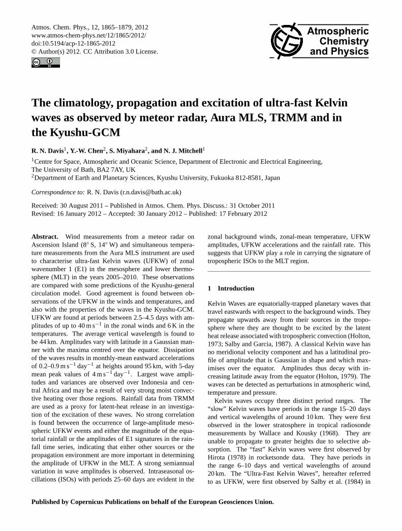
Fig. 1. Raw hourly(a) zonal and(b) meridional winds at a height of96 km from the Ascension Island radar with low-pass filtered windsoverlaid (dashed line) for the period 18–28 January 2005. The cut-off of the filter is 2.5 days. Note the oscillations in the zonal windswith period near 3 days.

87.5, 90.5, 93.5 and 97.0 km. The radar began operatingin May 2001, but for this study we have considered onlythe data overlapping the complete years available from AuraMLS, i.e. from 1 January 2005 to 31 December 2010. Thereare some significant gaps in the radar dataset amounting to22 % of 2005, 17 % of 2006, 71 % of 2007, 100 % of 2008,58 % of 2009 and 27 % of 2010.

Tropospheric convective heating may play a role in UFKWexcitation. Here we have used precipitation data from theTRMM “Multi-satellite Precipitation Analysis” dataset as aproxy for the latent heat release associated with troposphericconvection.

Finally, our observations are compared to the predictionsof the Kyushu-GCM T42L250 version. This model usestriangular-truncation at wavenumber 42 in the horizontal and250 layers in the vertical. The model covers heights fromthe ground up to approximately 150 km. In the MLT regionthe vertical resolution is∼500 m. The GCM includes short-and long-wave radiation processes, moist and dry convectiveadjustments, a local Richardson number dependent verticaleddy diffusion process and various other physical processes.Monthly-mean sea surface temperatures are used as a lowerboundary condition. The ground temperature is calculated inthe model by using its heat balance. No gravity-wave param-eterization is used, but a Rayleigh friction is imposed on thezonal-mean zonal winds to weaken the zonal winds aroundthe mesopause. More details can be found inChen and Miya-hara(2011).

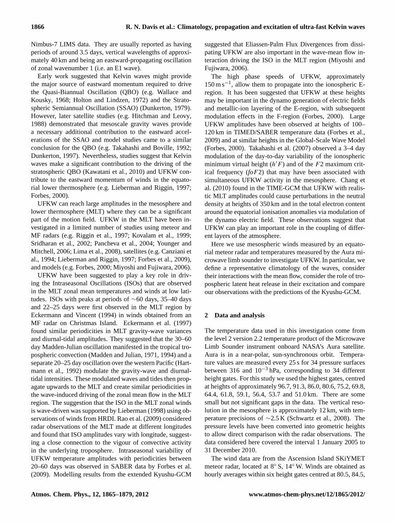
Fig. 2. Running Lomb-Scargle periodogram of(a) zonal and(b) meridional winds over Ascension Island for January–June 2005at a height of 96 km.

3 Results

3.1 Ascension Island meteor radar observations

Zonal winds measured over Ascension Island frequentlyshow wave-like oscillations with periods near 3–4 days. Asan example, Fig.1 presents hourly-mean zonal and merid-ional winds for a height of 96 km for the interval 18–28 Jan-uary 2005.

The figure shows a motion field dominated by a large-amplitude oscillation of period 24 h, which is the diurnal tide.Also present are lower-frequency oscillations. The dashedlines on the figure show the hourly winds low-pass filteredto reveal oscillations with periods longer than 2.5 days. Thefiltered winds reveal oscillations of period 3–4 days with am-plitudes reaching up to 30 m s−1 in the zonal component and20 m s−1 in the meridional component. The fact that theperiod of oscillation is about 3–4 days, combined with thelarger amplitudes in the zonal component, is a strong indi-cation that these winds are the signature of ultra-fast Kelvinwaves (note that there is also an indication of the 2-day wavein the meridional unfiltered winds).

To further investigate the possible presence of UFKW, adynamic spectrum of zonal and meridional winds was cal-culated for all six radar height gates and for all years of themeteor-radar data. Figure2 presents an example of theseresults for January–June 2005 for a height of 96 km. Thespectra were calculated using a Lomb-Scargle periodogramapplied to a data window of ten days, incremented throughthe dataset in steps of 1 day.

Considering the figure in detail it can be seen that eventswith period 3–4 days occur in an episodic manner and areparticularly noticeable in January–March 2005. Zonal windamplitudes regularly exceed 15 m s−1 and sometimes exceed

www.atmos-chem-phys.net/12/1865/2012/ Atmos. Chem. Phys., 12, 1865–1879, 2012

1868 R. N. Davis et al.: Climatology, propagation and excitation of ultra-fast Kelvin waves

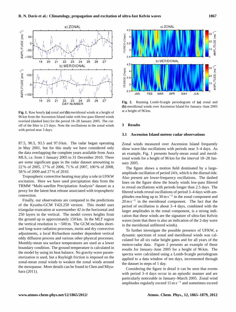
Fig. 3. Annually-averaged amplitude as a function of wave periodvs. height of E1 waves in the zonal wind at 2.1◦ N in the Kyushu-GCM.

30 m s−1 in the wave-period band 2.5–4.5 days associatedwith UFKW. When we consider the full dataset, we find peakamplitudes of up to 40 m s−1. Wave amplitudes and peri-ods vary greatly on timescales of a few days, demonstratingstrong intermittency. However, there is also a suggestion oflonger-term variability because wave amplitudes in January,February and March appear significantly larger than in April.These features of intermittency and stronger January–Marchactivity (and weaker April–June activity) are typical of allyears, however we will consider seasonal variability later.Meridional amplitudes can be large but are generally smallerthan the zonal amplitudes. For example, the largest zonalamplitudes in January and February are>30 m s−1 while thelargest meridional amplitudes are about 15 m s−1. This ob-servation, combined with the observed wave periods, pro-vides a strong indication that these spectral signatures resultfrom UFKW. Further, note that the theoretical suggestion thatUFKW have zero meridional velocities is actually based on asimplified set of assumptions and so UFKW observed awayfrom the equator may have non-zero meridional components.

The period range of UFKW in the MLT region can alsobe investigated in the Kyushu-GCM. The composite-yearperiod-height distribution of E1 wave amplitudes in themodel is presented in Fig.3. The figure shows that at heightsaround 95 km Kelvin waves have a period range of approx-imately 2–6 days with largest amplitudes between 2.5–4.5days. The GCM amplitudes seem low when compared toobservations but this is because they represent an annual-average, which due to the intermittency of the waves will in-clude intervals of little to no UFKW activity, which supressesthe average amplitudes.

We will hereafter interpret the 2.5–4.5 day oscillationsseen in the zonal spectra of Fig.2 as being due to UFKW(further justification for this assumption is provided by the si-multaneous observation of eastward-propagating oscillations

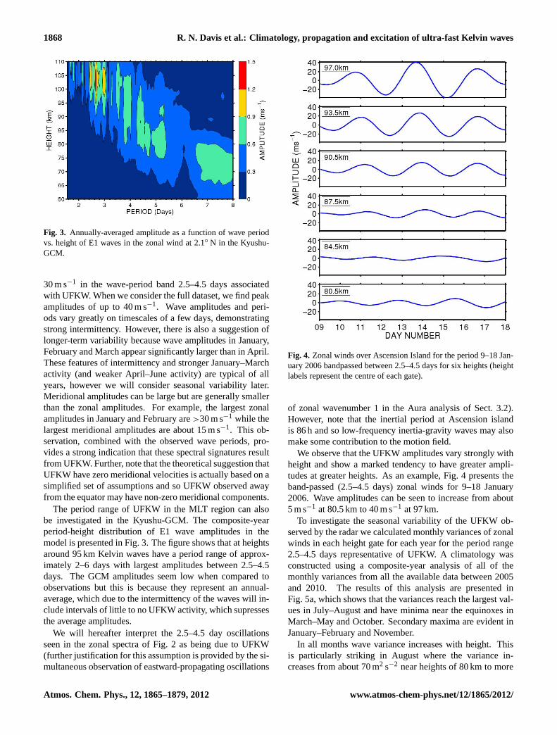
Fig. 4. Zonal winds over Ascension Island for the period 9–18 Jan-uary 2006 bandpassed between 2.5–4.5 days for six heights (heightlabels represent the centre of each gate).

of zonal wavenumber 1 in the Aura analysis of Sect. 3.2).However, note that the inertial period at Ascension islandis 86 h and so low-frequency inertia-gravity waves may alsomake some contribution to the motion field.

We observe that the UFKW amplitudes vary strongly withheight and show a marked tendency to have greater ampli-tudes at greater heights. As an example, Fig.4 presents theband-passed (2.5–4.5 days) zonal winds for 9–18 January2006. Wave amplitudes can be seen to increase from about5 m s−1 at 80.5 km to 40 m s−1 at 97 km.

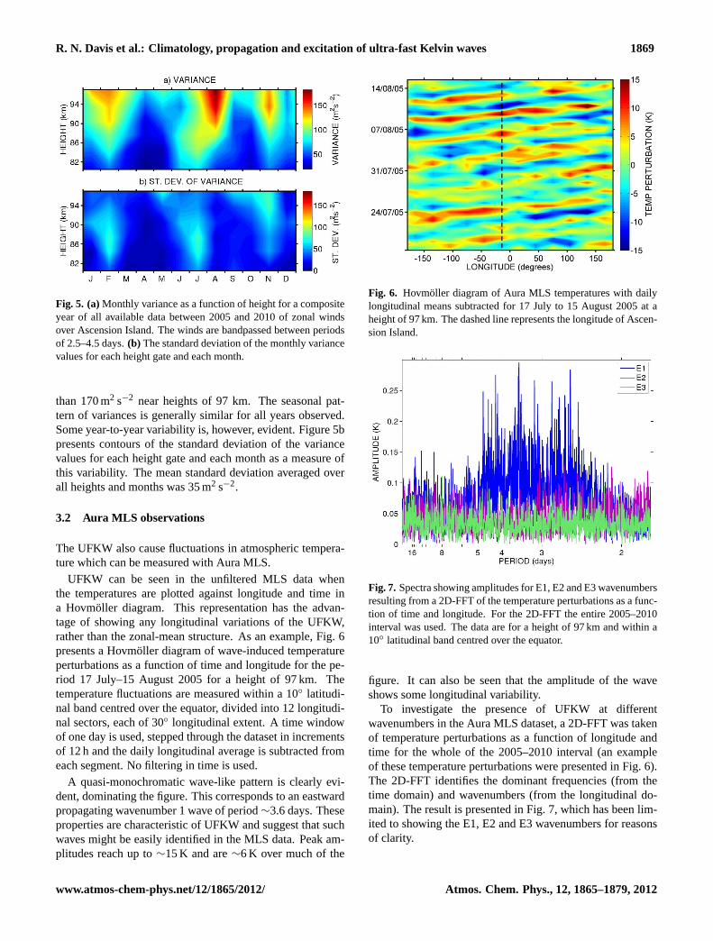
To investigate the seasonal variability of the UFKW ob-served by the radar we calculated monthly variances of zonalwinds in each height gate for each year for the period range2.5–4.5 days representative of UFKW. A climatology wasconstructed using a composite-year analysis of all of themonthly variances from all the available data between 2005and 2010. The results of this analysis are presented inFig. 5a, which shows that the variances reach the largest val-ues in July–August and have minima near the equinoxes inMarch–May and October. Secondary maxima are evident inJanuary–February and November.

In all months wave variance increases with height. Thisis particularly striking in August where the variance in-creases from about 70 m2 s−2 near heights of 80 km to more

Atmos. Chem. Phys., 12, 1865–1879, 2012 www.atmos-chem-phys.net/12/1865/2012/

R. N. Davis et al.: Climatology, propagation and excitation of ultra-fast Kelvin waves 1869

Fig. 5. (a)Monthly variance as a function of height for a compositeyear of all available data between 2005 and 2010 of zonal windsover Ascension Island. The winds are bandpassed between periodsof 2.5–4.5 days.(b) The standard deviation of the monthly variancevalues for each height gate and each month.

than 170 m2 s−2 near heights of 97 km. The seasonal pat-tern of variances is generally similar for all years observed.Some year-to-year variability is, however, evident. Figure5bpresents contours of the standard deviation of the variancevalues for each height gate and each month as a measure ofthis variability. The mean standard deviation averaged overall heights and months was 35 m2 s−2.

3.2 Aura MLS observations

The UFKW also cause fluctuations in atmospheric tempera-ture which can be measured with Aura MLS.

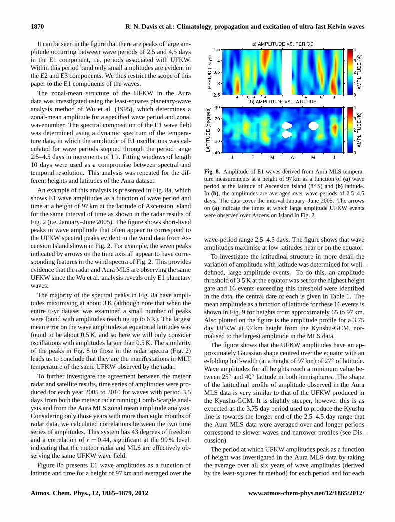
UFKW can be seen in the unfiltered MLS data whenthe temperatures are plotted against longitude and time ina Hovmoller diagram. This representation has the advan-tage of showing any longitudinal variations of the UFKW,rather than the zonal-mean structure. As an example, Fig.6presents a Hovmoller diagram of wave-induced temperatureperturbations as a function of time and longitude for the pe-riod 17 July–15 August 2005 for a height of 97 km. Thetemperature fluctuations are measured within a 10◦ latitudi-nal band centred over the equator, divided into 12 longitudi-nal sectors, each of 30◦ longitudinal extent. A time windowof one day is used, stepped through the dataset in incrementsof 12 h and the daily longitudinal average is subtracted fromeach segment. No filtering in time is used.

A quasi-monochromatic wave-like pattern is clearly evi-dent, dominating the figure. This corresponds to an eastwardpropagating wavenumber 1 wave of period∼3.6 days. Theseproperties are characteristic of UFKW and suggest that suchwaves might be easily identified in the MLS data. Peak am-plitudes reach up to∼15 K and are∼6 K over much of the

Fig. 6. Hovmoller diagram of Aura MLS temperatures with dailylongitudinal means subtracted for 17 July to 15 August 2005 at aheight of 97 km. The dashed line represents the longitude of Ascen-sion Island.

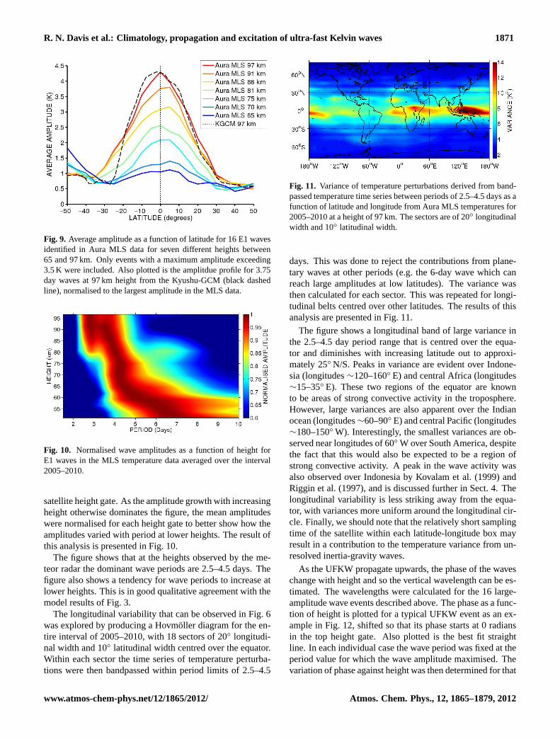
Fig. 7. Spectra showing amplitudes for E1, E2 and E3 wavenumbersresulting from a 2D-FFT of the temperature perturbations as a func-tion of time and longitude. For the 2D-FFT the entire 2005–2010interval was used. The data are for a height of 97 km and within a10◦ latitudinal band centred over the equator.

figure. It can also be seen that the amplitude of the waveshows some longitudinal variability.

To investigate the presence of UFKW at differentwavenumbers in the Aura MLS dataset, a 2D-FFT was takenof temperature perturbations as a function of longitude andtime for the whole of the 2005–2010 interval (an exampleof these temperature perturbations were presented in Fig.6).The 2D-FFT identifies the dominant frequencies (from thetime domain) and wavenumbers (from the longitudinal do-main). The result is presented in Fig.7, which has been lim-ited to showing the E1, E2 and E3 wavenumbers for reasonsof clarity.

www.atmos-chem-phys.net/12/1865/2012/ Atmos. Chem. Phys., 12, 1865–1879, 2012

1870 R. N. Davis et al.: Climatology, propagation and excitation of ultra-fast Kelvin waves

It can be seen in the figure that there are peaks of large am-plitude occurring between wave periods of 2.5 and 4.5 daysin the E1 component, i.e. periods associated with UFKW.Within this period band only small amplitudes are evident inthe E2 and E3 components. We thus restrict the scope of thispaper to the E1 components of the waves.

The zonal-mean structure of the UFKW in the Auradata was investigated using the least-squares planetary-waveanalysis method of Wu et al. (1995), which determines azonal-mean amplitude for a specified wave period and zonalwavenumber. The spectral composition of the E1 wave fieldwas determined using a dynamic spectrum of the tempera-ture data, in which the amplitude of E1 oscillations was cal-culated for wave periods stepped through the period range2.5–4.5 days in increments of 1 h. Fitting windows of length10 days were used as a compromise between spectral andtemporal resolution. This analysis was repeated for the dif-ferent heights and latitudes of the Aura dataset.

An example of this analysis is presented in Fig.8a, whichshows E1 wave amplitudes as a function of wave period andtime at a height of 97 km at the latitude of Ascension islandfor the same interval of time as shown in the radar results ofFig. 2 (i.e. January–June 2005). The figure shows short-livedpeaks in wave amplitude that often appear to correspond tothe UFKW spectral peaks evident in the wind data from As-cension Island shown in Fig.2. For example, the seven peaksindicated by arrows on the time axis all appear to have corre-sponding features in the wind spectra of Fig.2. This providesevidence that the radar and Aura MLS are observing the sameUFKW since the Wu et al. analysis reveals only E1 planetarywaves.

The majority of the spectral peaks in Fig.8a have ampli-tudes maximising at about 3 K (although note that when theentire 6-yr dataset was examined a small number of peakswere found with amplitudes reaching up to 6 K). The largestmean error on the wave amplitudes at equatorial latitudes wasfound to be about 0.5 K, and so here we will only consideroscillations with amplitudes larger than 0.5 K. The similarityof the peaks in Fig.8 to those in the radar spectra (Fig.2)leads us to conclude that they are the manifestations in MLTtemperature of the same UFKW observed by the radar.

To further investigate the agreement between the meteorradar and satellite results, time series of amplitudes were pro-duced for each year 2005 to 2010 for waves with period 3.5days from both the meteor radar running Lomb-Scargle anal-ysis and from the Aura MLS zonal mean amplitude analysis.Considering only those years with more than eight months ofradar data, we calculated correlations between the two timeseries of amplitudes. This system has 43 degrees of freedomand a correlation ofr = 0.44, significant at the 99 % level,indicating that the meteor radar and MLS are effectively ob-serving the same UFKW wave field.

Figure 8b presents E1 wave amplitudes as a function oflatitude and time for a height of 97 km and averaged over the

Fig. 8. Amplitude of E1 waves derived from Aura MLS tempera-ture measurements at a height of 97 km as a function of(a) waveperiod at the latitude of Ascension Island (8◦ S) and(b) latitude.In (b), the amplitudes are averaged over wave periods of 2.5–4.5days. The data cover the interval January–June 2005. The arrowson (a) indicate the times at which large amplitude UFKW eventswere observed over Ascension Island in Fig.2.

wave-period range 2.5–4.5 days. The figure shows that waveamplitudes maximise at low latitudes near or on the equator.

To investigate the latitudinal structure in more detail thevariation of amplitude with latitude was determined for well-defined, large-amplitude events. To do this, an amplitudethreshold of 3.5 K at the equator was set for the highest heightgate and 16 events exceeding this threshold were identifiedin the data, the central date of each is given in Table 1. Themean amplitude as a function of latitude for these 16 events isshown in Fig.9 for heights from approximately 65 to 97 km.Also plotted on the figure is the amplitude profile for a 3.75day UFKW at 97 km height from the Kyushu-GCM, nor-malised to the largest amplitude in the MLS data.

The figure shows that the UFKW amplitudes have an ap-proximately Gaussian shape centred over the equator with ane-folding half-width (at a height of 97 km) of 27◦ of latitude.Wave amplitudes for all heights reach a minimum value be-tween 25◦ and 40◦ latitude in both hemispheres. The shapeof the latitudinal profile of amplitude observed in the AuraMLS data is very similar to that of the UFKW produced inthe Kyushu-GCM. It is slightly steeper, however this is asexpected as the 3.75 day period used to produce the Kyushuline is towards the longer end of the 2.5–4.5 day range thatthe Aura MLS data were averaged over and longer periodscorrespond to slower waves and narrower profiles (see Dis-cussion).

The period at which UFKW amplitudes peak as a functionof height was investigated in the Aura MLS data by takingthe average over all six years of wave amplitudes (derivedby the least-squares fit method) for each period and for each

Atmos. Chem. Phys., 12, 1865–1879, 2012 www.atmos-chem-phys.net/12/1865/2012/

R. N. Davis et al.: Climatology, propagation and excitation of ultra-fast Kelvin waves 1871

Fig. 9. Average amplitude as a function of latitude for 16 E1 wavesidentified in Aura MLS data for seven different heights between65 and 97 km. Only events with a maximum amplitude exceeding3.5 K were included. Also plotted is the amplitdue profile for 3.75day waves at 97 km height from the Kyushu-GCM (black dashedline), normalised to the largest amplitude in the MLS data.

Fig. 10. Normalised wave amplitudes as a function of height forE1 waves in the MLS temperature data averaged over the interval2005–2010.

satellite height gate. As the amplitude growth with increasingheight otherwise dominates the figure, the mean amplitudeswere normalised for each height gate to better show how theamplitudes varied with period at lower heights. The result ofthis analysis is presented in Fig.10.

The figure shows that at the heights observed by the me-teor radar the dominant wave periods are 2.5–4.5 days. Thefigure also shows a tendency for wave periods to increase atlower heights. This is in good qualitative agreement with themodel results of Fig.3.

The longitudinal variability that can be observed in Fig.6was explored by producing a Hovmoller diagram for the en-tire interval of 2005–2010, with 18 sectors of 20◦ longitudi-nal width and 10◦ latitudinal width centred over the equator.Within each sector the time series of temperature perturba-tions were then bandpassed within period limits of 2.5–4.5

Fig. 11. Variance of temperature perturbations derived from band-passed temperature time series between periods of 2.5–4.5 days as afunction of latitude and longitude from Aura MLS temperatures for2005–2010 at a height of 97 km. The sectors are of 20◦ longitudinalwidth and 10◦ latitudinal width.

days. This was done to reject the contributions from plane-tary waves at other periods (e.g. the 6-day wave which canreach large amplitudes at low latitudes). The variance wasthen calculated for each sector. This was repeated for longi-tudinal belts centred over other latitudes. The results of thisanalysis are presented in Fig.11.

The figure shows a longitudinal band of large variance inthe 2.5–4.5 day period range that is centred over the equa-tor and diminishes with increasing latitude out to approxi-mately 25◦ N/S. Peaks in variance are evident over Indone-sia (longitudes∼120–160◦ E) and central Africa (longitudes∼15–35◦ E). These two regions of the equator are knownto be areas of strong convective activity in the troposphere.However, large variances are also apparent over the Indianocean (longitudes∼60–90◦ E) and central Pacific (longitudes∼180–150◦ W). Interestingly, the smallest variances are ob-served near longitudes of 60◦ W over South America, despitethe fact that this would also be expected to be a region ofstrong convective activity. A peak in the wave activity wasalso observed over Indonesia byKovalam et al.(1999) andRiggin et al.(1997), and is discussed further in Sect. 4. Thelongitudinal variability is less striking away from the equa-tor, with variances more uniform around the longitudinal cir-cle. Finally, we should note that the relatively short samplingtime of the satellite within each latitude-longitude box mayresult in a contribution to the temperature variance from un-resolved inertia-gravity waves.

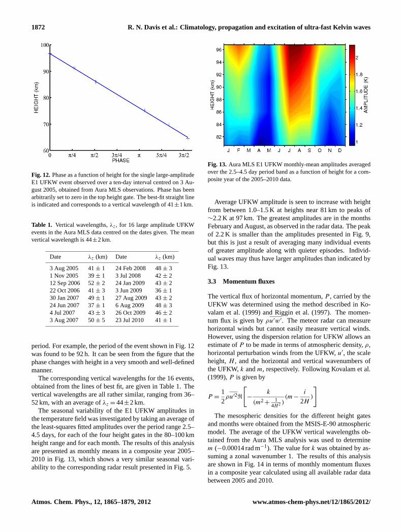
As the UFKW propagate upwards, the phase of the waveschange with height and so the vertical wavelength can be es-timated. The wavelengths were calculated for the 16 large-amplitude wave events described above. The phase as a func-tion of height is plotted for a typical UFKW event as an ex-ample in Fig.12, shifted so that its phase starts at 0 radiansin the top height gate. Also plotted is the best fit straightline. In each individual case the wave period was fixed at theperiod value for which the wave amplitude maximised. Thevariation of phase against height was then determined for that

www.atmos-chem-phys.net/12/1865/2012/ Atmos. Chem. Phys., 12, 1865–1879, 2012

1872 R. N. Davis et al.: Climatology, propagation and excitation of ultra-fast Kelvin waves

Fig. 12.Phase as a function of height for the single large-amplitudeE1 UFKW event observed over a ten-day interval centred on 3 Au-gust 2005, obtained from Aura MLS observations. Phase has beenarbitrarily set to zero in the top height gate. The best-fit straight lineis indicated and corresponds to a vertical wavelength of 41±1 km.

Table 1. Vertical wavelengths,λz, for 16 large amplitude UFKWevents in the Aura MLS data centred on the dates given. The meanvertical wavelength is 44±2 km.

Date λz (km) Date λz (km)

3 Aug 2005 41± 1 24 Feb 2008 48± 31 Nov 2005 39± 1 3 Jul 2008 42± 212 Sep 2006 52± 2 24 Jan 2009 43± 222 Oct 2006 41± 3 3 Jun 2009 36± 130 Jan 2007 49± 1 27 Aug 2009 43± 224 Jun 2007 37± 1 6 Aug 2009 48± 34 Jul 2007 43± 3 26 Oct 2009 46± 23 Aug 2007 50± 5 23 Jul 2010 41± 1

period. For example, the period of the event shown in Fig.12was found to be 92 h. It can be seen from the figure that thephase changes with height in a very smooth and well-definedmanner.

The corresponding vertical wavelengths for the 16 events,obtained from the lines of best fit, are given in Table 1. Thevertical wavelengths are all rather similar, ranging from 36–52 km, with an average ofλz = 44±2 km.

The seasonal variability of the E1 UFKW amplitudes inthe temperature field was investigated by taking an average ofthe least-squares fitted amplitudes over the period range 2.5–4.5 days, for each of the four height gates in the 80–100 kmheight range and for each month. The results of this analysisare presented as monthly means in a composite year 2005–2010 in Fig.13, which shows a very similar seasonal vari-ability to the corresponding radar result presented in Fig.5.

Fig. 13. Aura MLS E1 UFKW monthly-mean amplitudes averagedover the 2.5–4.5 day period band as a function of height for a com-posite year of the 2005–2010 data.

Average UFKW amplitude is seen to increase with heightfrom between 1.0–1.5 K at heights near 81 km to peaks of∼2.2 K at 97 km. The greatest amplitudes are in the monthsFebruary and August, as observed in the radar data. The peakof 2.2 K is smaller than the amplitudes presented in Fig.9,but this is just a result of averaging many individual eventsof greater amplitude along with quieter episodes. Individ-ual waves may thus have larger amplitudes than indicated byFig. 13.

3.3 Momentum fluxes

The vertical flux of horizontal momentum,P , carried by theUFKW was determined using the method described inKo-valam et al.(1999) andRiggin et al.(1997). The momen-tum flux is given byρu′w′. The meteor radar can measurehorizontal winds but cannot easily measure vertical winds.However, using the dispersion relation for UFKW allows anestimate ofP to be made in terms of atmospheric density,ρ,horizontal perturbation winds from the UFKW,u′, the scaleheight,H , and the horizontal and vertical wavenumbers ofthe UFKW,k andm, respectively. FollowingKovalam et al.(1999), P is given by

P =1

2ρu′2<

[−

k

(m2+1

4H2 )(m−

i

2H)

]The mesospheric densities for the different height gates

and months were obtained from the MSIS-E-90 atmosphericmodel. The average of the UFKW vertical wavelengths ob-tained from the Aura MLS analysis was used to determinem (−0.00014 rad m−1). The value fork was obtained by as-suming a zonal wavenumber 1. The results of this analysisare shown in Fig.14 in terms of monthly momentum fluxesin a composite year calculated using all available radar databetween 2005 and 2010.

Atmos. Chem. Phys., 12, 1865–1879, 2012 www.atmos-chem-phys.net/12/1865/2012/

R. N. Davis et al.: Climatology, propagation and excitation of ultra-fast Kelvin waves 1873

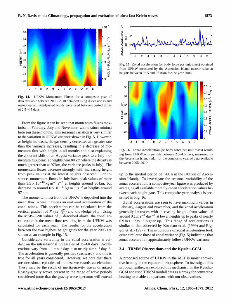
Fig. 14. UFKW Momentum Fluxes for a composite year ofdata available between 2005–2010 obtained using Ascension Islandmeteor-radar. Bandpassed winds were used between period limitsof 2.5–4.5 days.

From the figure it can be seen that momentum fluxes max-imise in February, July and November, with distinct minimabetween these months. This seasonal variation is very similarto the variation in UFKW variance shown in Fig.5. However,as height increases, the gas density decreases at a greater ratethan the variance increases, resulting in a decrease of mo-mentum flux with height in all months and also explainingthe apparent shift of an August variance peak to a July mo-mentum flux peak (at heights near 80 km where the density ismuch greater than at 97 km, the variance peaks in July). Themomentum fluxes decrease strongly with increasing heightfrom peak values at the lowest heights observed. For in-stance, momentum fluxes in July have peak values of morethan 3.5× 10−10 kg m−1 s−2 at heights around 80 km, butdecrease to around 6× 10−11 kg m−1 s−2 at heights around97 km.

The momentum lost from the UFKW is deposited into themean flow, where it causes an eastward acceleration of thezonal winds. This acceleration can be calculated from thevertical gradient ofP (i.e. dP

dz) and knowledge ofρ. Using

the MSIS-E-90 values ofρ described above, the zonal ac-celeration in the mean flow resulting from the UFKW wascalculated for each year. The results for the accelerationbetween the two highest height gates for the year 2006 areshown as an example in Fig.15.

Considerable variability in the zonal acceleration is evi-dent on the intraseasonal timescales of 25–60 days. Accel-erations vary from−1 m s−1 day−1 to nearly 4 m s−1 day−1.The acceleration is generally positive (eastward), and this istrue for all years considered. However, we note that thereare occasional episodes of modest westwards acceleration.These may be the result of inertia-gravity waves or mixedRossby-gravity waves present in the range of wave periodsconsidered (note that the gravity wave spectrum will extend

Fig. 15. Zonal acceleration (or body force per unit mass) obtainedfrom UFKW measured by the Ascension Island meteor-radar atheights between 93.5 and 97.0 km for the year 2006.

Fig. 16. Zonal Acceleration (or body force per unit mass) result-ing from UFKW with periods between 2.5–4.5 days, measured bythe Ascension Island radar for the composite year of data availablebetween 2005–2010.

up to the inertial period of∼86 h at the latitude of Ascen-sion Island). To investigate the seasonal variability of thezonal acceleration, a composite-year figure was produced byaveraging all available monthly-mean acceleration values be-tween each height gate. This composite year analysis is pre-sented in Fig.16.

Zonal accelerations are seen to have maximum values inFebruary, August and November, and the zonal accelerationgenerally increases with increasing height, from values ofaround 0.1 m s−1 day−1 at lower heights up to peaks of nearly0.9 m s−1 day−1 higher up. This range of accelerations issimilar to that observed byKovalam et al.(1999) andRig-gin et al.(1997). These contours of zonal acceleration lookquite similar to those of zonal variance (Fig.5) indicating thatzonal acceleration approximately follows UFKW variance.

3.4 TRMM Observations and the Kyushu-GCM

A proposed source of UFKW in the MLT is moist convec-tive heating in the equatorial troposphere. To investigate thisproposal further, we explored this mechanism in the Kyushu-GCM and used TRMM rainfall data as a proxy for convectiveheating to enable comparisons with our observations.

www.atmos-chem-phys.net/12/1865/2012/ Atmos. Chem. Phys., 12, 1865–1879, 2012

1874 R. N. Davis et al.: Climatology, propagation and excitation of ultra-fast Kelvin waves

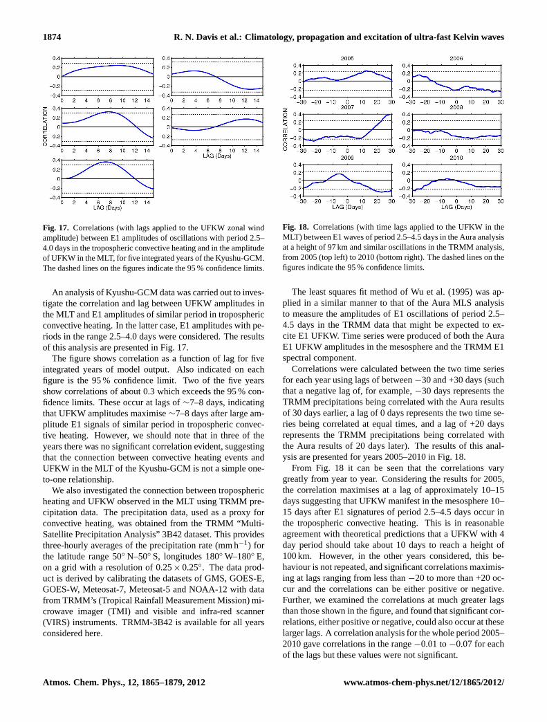
Fig. 17. Correlations (with lags applied to the UFKW zonal windamplitude) between E1 amplitudes of oscillations with period 2.5–4.0 days in the tropospheric convective heating and in the amplitudeof UFKW in the MLT, for five integrated years of the Kyushu-GCM.The dashed lines on the figures indicate the 95 % confidence limits.

An analysis of Kyushu-GCM data was carried out to inves-tigate the correlation and lag between UFKW amplitudes inthe MLT and E1 amplitudes of similar period in troposphericconvective heating. In the latter case, E1 amplitudes with pe-riods in the range 2.5–4.0 days were considered. The resultsof this analysis are presented in Fig.17.

The figure shows correlation as a function of lag for fiveintegrated years of model output. Also indicated on eachfigure is the 95 % confidence limit. Two of the five yearsshow correlations of about 0.3 which exceeds the 95 % con-fidence limits. These occur at lags of∼7–8 days, indicatingthat UFKW amplitudes maximise∼7–8 days after large am-plitude E1 signals of similar period in tropospheric convec-tive heating. However, we should note that in three of theyears there was no significant correlation evident, suggestingthat the connection between convective heating events andUFKW in the MLT of the Kyushu-GCM is not a simple one-to-one relationship.

We also investigated the connection between troposphericheating and UFKW observed in the MLT using TRMM pre-cipitation data. The precipitation data, used as a proxy forconvective heating, was obtained from the TRMM “Multi-Satellite Precipitation Analysis” 3B42 dataset. This providesthree-hourly averages of the precipitation rate (mm h−1) forthe latitude range 50◦ N–50◦ S, longitudes 180◦ W–180◦ E,on a grid with a resolution of 0.25× 0.25◦. The data prod-uct is derived by calibrating the datasets of GMS, GOES-E,GOES-W, Meteosat-7, Meteosat-5 and NOAA-12 with datafrom TRMM’s (Tropical Rainfall Measurement Mission) mi-crowave imager (TMI) and visible and infra-red scanner(VIRS) instruments. TRMM-3B42 is available for all yearsconsidered here.

Fig. 18. Correlations (with time lags applied to the UFKW in theMLT) between E1 waves of period 2.5–4.5 days in the Aura analysisat a height of 97 km and similar oscillations in the TRMM analysis,from 2005 (top left) to 2010 (bottom right). The dashed lines on thefigures indicate the 95 % confidence limits.

The least squares fit method of Wu et al. (1995) was ap-plied in a similar manner to that of the Aura MLS analysisto measure the amplitudes of E1 oscillations of period 2.5–4.5 days in the TRMM data that might be expected to ex-cite E1 UFKW. Time series were produced of both the AuraE1 UFKW amplitudes in the mesosphere and the TRMM E1spectral component.

Correlations were calculated between the two time seriesfor each year using lags of between−30 and +30 days (suchthat a negative lag of, for example,−30 days represents theTRMM precipitations being correlated with the Aura resultsof 30 days earlier, a lag of 0 days represents the two time se-ries being correlated at equal times, and a lag of +20 daysrepresents the TRMM precipitations being correlated withthe Aura results of 20 days later). The results of this anal-ysis are presented for years 2005–2010 in Fig.18.

From Fig. 18 it can be seen that the correlations varygreatly from year to year. Considering the results for 2005,the correlation maximises at a lag of approximately 10–15days suggesting that UFKW manifest in the mesosphere 10–15 days after E1 signatures of period 2.5–4.5 days occur inthe tropospheric convective heating. This is in reasonableagreement with theoretical predictions that a UFKW with 4day period should take about 10 days to reach a height of100 km. However, in the other years considered, this be-haviour is not repeated, and significant correlations maximis-ing at lags ranging from less than−20 to more than +20 oc-cur and the correlations can be either positive or negative.Further, we examined the correlations at much greater lagsthan those shown in the figure, and found that significant cor-relations, either positive or negative, could also occur at theselarger lags. A correlation analysis for the whole period 2005–2010 gave correlations in the range−0.01 to−0.07 for eachof the lags but these values were not significant.

Atmos. Chem. Phys., 12, 1865–1879, 2012 www.atmos-chem-phys.net/12/1865/2012/

R. N. Davis et al.: Climatology, propagation and excitation of ultra-fast Kelvin waves 1875

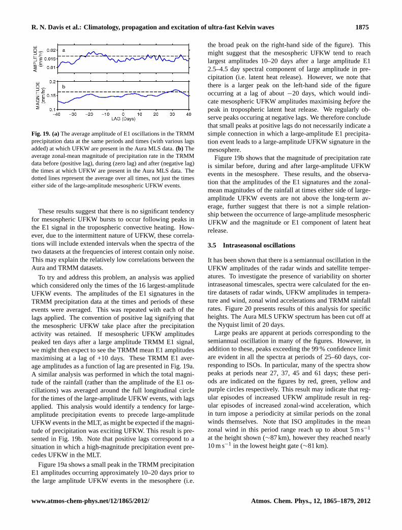
Fig. 19. (a)The average amplitude of E1 oscillations in the TRMMprecipitation data at the same periods and times (with various lagsadded) at which UFKW are present in the Aura MLS data.(b) Theaverage zonal-mean magnitude of precipitation rate in the TRMMdata before (positive lag), during (zero lag) and after (negative lag)the times at which UFKW are present in the Aura MLS data. Thedotted lines represent the average over all times, not just the timeseither side of the large-amplitude mesospheric UFKW events.

These results suggest that there is no significant tendencyfor mesospheric UFKW bursts to occur following peaks inthe E1 signal in the tropospheric convective heating. How-ever, due to the intermittent nature of UFKW, these correla-tions will include extended intervals when the spectra of thetwo datasets at the frequencies of interest contain only noise.This may explain the relatively low correlations between theAura and TRMM datasets.

To try and address this problem, an analysis was appliedwhich considered only the times of the 16 largest-amplitudeUFKW events. The amplitudes of the E1 signatures in theTRMM precipitation data at the times and periods of theseevents were averaged. This was repeated with each of thelags applied. The convention of positive lag signifying thatthe mesospheric UFKW take place after the precipitationactivity was retained. If mesospheric UFKW amplitudespeaked ten days after a large amplitude TRMM E1 signal,we might then expect to see the TRMM mean E1 amplitudesmaximising at a lag of +10 days. These TRMM E1 aver-age amplitudes as a function of lag are presented in Fig.19a.A similar analysis was performed in which the total magni-tude of the rainfall (rather than the amplitude of the E1 os-cillations) was averaged around the full longitudinal circlefor the times of the large-amplitude UFKW events, with lagsapplied. This analysis would identify a tendency for large-amplitude precipitation events to precede large-amplitudeUFKW events in the MLT, as might be expected if the magni-tude of precipitation was exciting UFKW. This result is pre-sented in Fig.19b. Note that positive lags correspond to asituation in which a high-magnitude precipitation event pre-cedes UFKW in the MLT.

Figure19a shows a small peak in the TRMM precipitationE1 amplitudes occurring approximately 10–20 days prior tothe large amplitude UFKW events in the mesosphere (i.e.

the broad peak on the right-hand side of the figure). Thismight suggest that the mesospheric UFKW tend to reachlargest amplitudes 10–20 days after a large amplitude E12.5–4.5 day spectral component of large amplitude in pre-cipitation (i.e. latent heat release). However, we note thatthere is a larger peak on the left-hand side of the figureoccurring at a lag of about−20 days, which would indi-cate mesospheric UFKW amplitudes maximisingbeforethepeak in tropospheric latent heat release. We regularly ob-serve peaks occuring at negative lags. We therefore concludethat small peaks at positive lags do not necessarily indicate asimple connection in which a large-amplitude E1 precipita-tion event leads to a large-amplitude UFKW signature in themesosphere.

Figure19b shows that the magnitude of precipitation rateis similar before, during and after large-amplitude UFKWevents in the mesosphere. These results, and the observa-tion that the amplitudes of the E1 signatures and the zonal-mean magnitudes of the rainfall at times either side of large-amplitude UFKW events are not above the long-term av-erage, further suggest that there is not a simple relation-ship between the occurrence of large-amplitude mesosphericUFKW and the magnitude or E1 component of latent heatrelease.

3.5 Intraseasonal oscillations

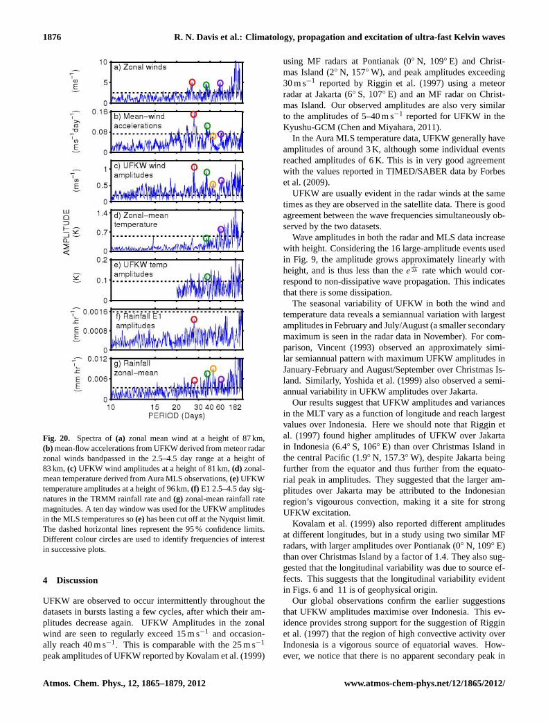
It has been shown that there is a semiannual oscillation in theUFKW amplitudes of the radar winds and satellite temper-atures. To investigate the presence of variability on shorterintraseasonal timescales, spectra were calculated for the en-tire datasets of radar winds, UFKW amplitudes in tempera-ture and wind, zonal wind accelerations and TRMM rainfallrates. Figure20 presents results of this analysis for specificheights. The Aura MLS UFKW spectrum has been cut off atthe Nyquist limit of 20 days.

Large peaks are apparent at periods corresponding to thesemiannual oscillation in many of the figures. However, inaddition to these, peaks exceeding the 99 % confidence limitare evident in all the spectra at periods of 25–60 days, cor-responding to ISOs. In particular, many of the spectra showpeaks at periods near 27, 37, 45 and 61 days; these peri-ods are indicated on the figures by red, green, yellow andpurple circles respectively. This result may indicate that reg-ular episodes of increased UFKW amplitude result in reg-ular episodes of increased zonal-wind acceleration, whichin turn impose a periodicity at similar periods on the zonalwinds themselves. Note that ISO amplitudes in the meanzonal wind in this period range reach up to about 5 m s−1

at the height shown (∼87 km), however they reached nearly10 m s−1 in the lowest height gate (∼81 km).

www.atmos-chem-phys.net/12/1865/2012/ Atmos. Chem. Phys., 12, 1865–1879, 2012

1876 R. N. Davis et al.: Climatology, propagation and excitation of ultra-fast Kelvin waves

Fig. 20. Spectra of(a) zonal mean wind at a height of 87 km,(b) mean-flow accelerations from UFKW derived from meteor radarzonal winds bandpassed in the 2.5–4.5 day range at a height of83 km,(c) UFKW wind amplitudes at a height of 81 km,(d) zonal-mean temperature derived from Aura MLS observations,(e)UFKWtemperature amplitudes at a height of 96 km,(f) E1 2.5–4.5 day sig-natures in the TRMM rainfall rate and(g) zonal-mean rainfall ratemagnitudes. A ten day window was used for the UFKW amplitudesin the MLS temperatures so(e)has been cut off at the Nyquist limit.The dashed horizontal lines represent the 95 % confidence limits.Different colour circles are used to identify frequencies of interestin successive plots.

4 Discussion

UFKW are observed to occur intermittently throughout thedatasets in bursts lasting a few cycles, after which their am-plitudes decrease again. UFKW Amplitudes in the zonalwind are seen to regularly exceed 15 m s−1 and occasion-ally reach 40 m s−1. This is comparable with the 25 m s−1

peak amplitudes of UFKW reported byKovalam et al.(1999)

using MF radars at Pontianak (0◦ N, 109◦ E) and Christ-mas Island (2◦ N, 157◦ W), and peak amplitudes exceeding30 m s−1 reported byRiggin et al. (1997) using a meteorradar at Jakarta (6◦ S, 107◦ E) and an MF radar on Christ-mas Island. Our observed amplitudes are also very similarto the amplitudes of 5–40 m s−1 reported for UFKW in theKyushu-GCM (Chen and Miyahara, 2011).

In the Aura MLS temperature data, UFKW generally haveamplitudes of around 3 K, although some individual eventsreached amplitudes of 6 K. This is in very good agreementwith the values reported in TIMED/SABER data byForbeset al.(2009).

UFKW are usually evident in the radar winds at the sametimes as they are observed in the satellite data. There is goodagreement between the wave frequencies simultaneously ob-served by the two datasets.

Wave amplitudes in both the radar and MLS data increasewith height. Considering the 16 large-amplitude events usedin Fig. 9, the amplitude grows approximately linearly withheight, and is thus less than thee

z2h rate which would cor-

respond to non-dissipative wave propagation. This indicatesthat there is some dissipation.

The seasonal variability of UFKW in both the wind andtemperature data reveals a semiannual variation with largestamplitudes in February and July/August (a smaller secondarymaximum is seen in the radar data in November). For com-parison, Vincent (1993) observed an approximately simi-lar semiannual pattern with maximum UFKW amplitudes inJanuary-February and August/September over Christmas Is-land. Similarly,Yoshida et al.(1999) also observed a semi-annual variability in UFKW amplitudes over Jakarta.

Our results suggest that UFKW amplitudes and variancesin the MLT vary as a function of longitude and reach largestvalues over Indonesia. Here we should note thatRiggin etal. (1997) found higher amplitudes of UFKW over Jakartain Indonesia (6.4◦ S, 106◦ E) than over Christmas Island inthe central Pacific (1.9◦ N, 157.3◦ W), despite Jakarta beingfurther from the equator and thus further from the equato-rial peak in amplitudes. They suggested that the larger am-plitudes over Jakarta may be attributed to the Indonesianregion’s vigourous convection, making it a site for strongUFKW excitation.

Kovalam et al.(1999) also reported different amplitudesat different longitudes, but in a study using two similar MFradars, with larger amplitudes over Pontianak (0◦ N, 109◦ E)than over Christmas Island by a factor of 1.4. They also sug-gested that the longitudinal variability was due to source ef-fects. This suggests that the longitudinal variability evidentin Figs.6 and 11 is of geophysical origin.

Our global observations confirm the earlier suggestionsthat UFKW amplitudes maximise over Indonesia. This ev-idence provides strong support for the suggestion ofRigginet al. (1997) that the region of high convective activity overIndonesia is a vigorous source of equatorial waves. How-ever, we notice that there is no apparent secondary peak in

Atmos. Chem. Phys., 12, 1865–1879, 2012 www.atmos-chem-phys.net/12/1865/2012/

R. N. Davis et al.: Climatology, propagation and excitation of ultra-fast Kelvin waves 1877

UFKW variances over the convective region of South Amer-ica. However, our observation that this longitudinal peak invariance is not evident at latitudes away from the equator(where the inertial period limit falls out of the 2.5–4.5 dayrange) may still suggest that waves other than UFKW arecontributing to this maximum.

The variation of amplitude with latitude evident in Fig.9is approximately gaussian and maximises over the equatorwith an e-folding half-width of∼27◦ of latitude. Followingthe work ofHolton and Lindzen(1968) the e-folding half-width of Kelvin waves can be shown to be

Ly '

√2ω

βk

where for the beta-plane centred over the equatorβ =2�rE

,

for the Earth’s rotation rate� (in rad s−1) and Earth’s radiusrE. UFKW of zonal wavenumber 1 and period of 3.5 days(the average period of the 16 large-amplitude events includedin Fig. 9) have zonal phase speeds ofω

k' 130 m s−1. This

corresponds to a predicted half-width ofLy ' 3400 km, or30.5◦ of latitude. This is remarkably close to our observedresult of∼27◦ of latitude and further confirms our inferencethat the analysis is detecting UFKW.

The average vertical wavelength of Table 1,λz = 44±

2 km, is consistent with the averageλz values of 41 km foundby Salby et al.(1984), and 43 km found by bothSridharan etal. (2002) andLima et al. (2008), but considerably shorterthan the values of 87 and 116 km reported byRiggin et al.(1997) and values between 53 and 88 km observed byKo-valam et al.(1999). A wave of wavenumber 1 travellingaround the equator would have a horizontal wavelength ap-proximately equal to the circumference of the equator, i.e.λx = 40 700 km. Using the Kelvin wave dispersion relation,

λz = TB

[λx

τ−u

],

and using values ofTB ' 300 s for the MLT region Brunt-Vaisala period andu = 0 m s−1 as an approximation for themean wind (Forbes et al., 2009) we obtain vertical wave-lengths ranging from 31.4 to 56.5 km for UFKW with periodsτ = 2.5–4.5 days. These numbers are in excellent agreementwith the observations presented in Table 1.

As UFKW dissipate, they deposit their eastward momen-tum into the mean flow, creating an eastward acceleration.The accelerations measured here (Figs.15and16) are seen tobe almost always eastward. The range of monthly-mean val-ues at heights near 95 km of∼0.2–0.9 m s−1 day−1, is sim-ilar to that obtained from radar measurements at Pontianak(Kovalam et al., 1999). The average monthly mean valueof 0.44 m s−1 day−1 is slightly greater than that obtained atChristmas Island of 0.32 m s−1 day−1, but less than that ob-tained at Jakarta of 0.67 m s−1 day−1 (Riggin et al., 1997).Peak accelerations associated with large events can reach upto ∼4 m s−1 day−1. This suggests that UFKW make a small

contribution to the equatorial MLT region when comparedto, for example, the contribution of gravity waves at midlati-tudes (e.g.Norton and Thuburn, 1999).

In Sect. 3.4 we considered correlations between tropo-spheric rainfall parameters and UFKW amplitudes in theMLT. Although in 2005 there was a peak in the correlationat lags of 10–20 days that is significant at the 95 % level, inother years the correlation at these lags was actually weaklynegative. These low correlation values might be due to theepisodic nature of the UFKW, as the time series being corre-lated will include long intervals of time during which thereis little to no activity, and so noise would reduce the cor-relations. However, we might still have expected that themagnitude or the average amplitude of E1 signatures in therainfall would be larger than average before the occurrenceof a burst of mesospheric UFKW. However, this was not ob-served. These observations suggest that there is no simplerelationship between these rainfall parameters and the occur-rence of large-amplitude UFKW in the MLT. Nevertheless,the results presented in Fig.20 suggest a link between ISOsin the rainfall and ISOs in the mesospheric UFKW ampli-tudes.

ISOs were found in the two rainfall parameters considered,in the UFKW amplitudes and mean-flow accelerations, back-ground zonal winds and zonal-mean temperatures with clus-ters of spectral peaks at periods in the 30–60 day range asso-ciated with the Madden-Julian oscillation and the 20–25 dayrange associated with the oscillation reported byHartmann etal. (1992) (Fig. 20). Similar observations of ISOs in UFKWtemperature amplitudes and zonal-mean temperature havebeen reported byForbes et al.(2009) in TIMED/SABERdata. Our results suggest that ISOs in zonal-mean rainfall(a proxy for tropospheric convective heating) result in mod-ulation of UFKW amplitudes in the MLT at similar periods.This in turn modulates the mean-wind accelerations causedby the dissipation of those UFKW. It is interesting to notethat the zonal winds also show periodicities that match wellwith those of the mean-wind accelerations, from which onemight infer that these oscillations in the mean wind were be-ing driven by the momentum deposition from UFKW. How-ever, we should note that ISOs are also know to exist ingravity-wave and diurnal-tidal amplitudes (Miyoshi and Fu-jiwara, 2006; Eckermann et al., 1997) which can also con-tribute to ISOs in the zonal winds. The relative role ofUFKW, gravity waves and tides in exciting mean wind ISOsin the MLT thus remains to be determined.

5 Conclusions

Winds from the Ascension Island meteor radar (8◦ S, 14◦ W)and temperatures recorded simultaneously by the Aura MLSinstrument have been analysed to characterise ultra-fastKelvin waves of period 2.5–4.5 days at equatorial latitudesand at heights of up to∼100 km. These have been compared

www.atmos-chem-phys.net/12/1865/2012/ Atmos. Chem. Phys., 12, 1865–1879, 2012

1878 R. N. Davis et al.: Climatology, propagation and excitation of ultra-fast Kelvin waves

with observations made from the Kyushu-GCM and in theTRMM rainfall data. Our conclusions are as follows:

1. Clear but intermittent UFKW are observed with zonalwind amplitudes reaching up to 40 m s−1 and tempera-ture amplitudes of up to 6 K. The average vertical wave-length isλz = 44±2 km. The variation of UFKW am-plitude with latitude is observed to be approximatelygaussian with an e-folding half-width of 27◦ of latitude.

2. There is good agreement of UFKW observations in theradar zonal winds and in the Aura MLS temperatures,with UFKW found simultaneously at the same frequen-cies in both datasets.

3. Amplitudes do not grow at the exponential free growthrate with height which means that the waves dissipate,depositing eastward momentum into the mean flow.Monthly mean acceleration values are found to be 0.2–0.9 m s−1 day−1 at heights near 95 km.

4. A semiannual variation in wave amplitude is evident inboth datasets with largest amplitudes in February andJuly/August.

5. A longitudinal variability is found in the variance oftemperature perturbations associated with these waveswith largest values over Indonesia and Africa. This isattributed to the strong tropospheric convection of theseregions. The absence of a peak in activity over SouthAmerica is unexplained.

6. No clear link is found between the occurrence of large-amplitude mesospheric UFKW and E1 signatures inrainfall or zonal-mean magnitude of rainfall.

7. ISOs with periods between∼25–60 days are observedin the long-term spectra for the mean zonal winds, thezonal-mean temperatures, the UFKW amplitudes andassociated mean-flow accelerations, and in the rainfallmagnitudes. This supports the suggestion that the tro-pospheric Madden-Julian oscillation and the 20–25 dayoscillation ofHartmann et al.(1992) modulate the inten-sity of UFKW, which then propagate upwards and con-tribute to similar periodicities in the background windsby wave-mean flow interactions. However, the relativerole of UFKW, gravity-waves and tides in driving ISOsin the zonal winds has yet to be determined.

Edited by: A. J. G. Baumgaertner

References

Canziani, P. O., Holton, J. R., Fishbein, E., Froidevaux, L.,and Waters, J. W.: Equatorial Kelvin waves – a UARSMLS view, J. Atmos. Sci., 51, 3053–3076,doi:10.1175/1520-0469(1994)051<3053:EKWAUM>2.0.CO;2, 1994.

Chang, L. C., Palo, S. E., Liu, H. L., Fang, T. W., and Lin, C.S.: Response of the thermosphere and ionosphere to an ul-tra fast Kelvin wave, J. Geophys. Res.-Space, 115, A00G04,doi:10.1029/2010JA015453, 2010.

Chen, Y.-W. and Miyahara, S.: Analysis of fast and ultra-fast Kelvinwaves simulated by the Kyushu-GCM, J. Atmos. Sol.-Terr. Phy.,submitted, 2011.

Dunkerton, T. J.: Role of the Kelvin wave in the westerly phase ofthe semiannual zonal wind oscillation, J. Atmos. Sci., 36, 32–41,doi:10.1175/1520-0469(1979)036<0032:OTROTK>2.0.CO;2,1979.

Dunkerton, T. J.: The role of gravity waves in the quasi-biennial oscillation, J. Geophys. Res.-Atmos., 102, 26053–26076,doi:10.1029/96JD02999, 1997.

Eckermann, S. D. and Vincent, R. A.: 1st observations ofintraseasonal oscillations in the equatorial mesosphere andlower thermosphere, Geophys. Res. Lett., 21, 265–268,doi:10.1029/93GL02835, 1994.

Eckermann, S. D., Rajopadhyaya, D. K., and Vincent, R.A.: Intraseasonal wind variability in the equatorial meso-sphere and lower thermosphere: Long-term observations fromthe central Pacific, J. Atmos. Sol.-Terr. Phy., 59, 603–627,doi:10.1016/S1364-6826(96)00143-5, 1997.

Forbes, J. M.: Wave coupling between the lower and upper atmo-sphere: case study of an ultra-fast Kelvin Wave, J. Atmos. Sol.-Terr. Phy., 62, 1603–1621,doi:10.1016/S1364-6826(00)00115-2, 2000.

Forbes, J. M., Zhang, X. L., Palo, S. E., Russell, J., Mertens,C. J., and Mlynczak, M.: Kelvin waves in stratosphere, meso-sphere and lower thermosphere temperatures as observed byTIMED/SABER during 2002–2006, Earth Planets Space, 61,447–453, 2009.

Hartmann, D. L., Michelsen, M. L., and Klein, S. A.: Seasonal-variations of tropical intraseasonal oscillations – a 20–25 dayoscillation in the western Pacific, J. Atmos. Sci., 49, 1277–1289,doi:10.1175/1520-0469(1992)049<1277:SVOTIO>2.0.CO;2,1992.

Hirota, I.: Equatorial waves in upper stratosphere and meso-sphere in relation to semiannual oscillation of zonalwind, J. Atmos. Sci., 35, 714–722,doi:10.1175/1520-0469(1978)035<0714:EWITUS>2.0.CO;2, 1978.

Hitchman, M. H. and Leovy, C. B.: Estimation of theKelvin wave contribution to the Semiannual Oscilla-tion, J. Atmos. Sci., 45, 1462–1475,doi:10.1175/1520-0469(1988)045<1462:EOTKWC>2.0.CO;2, 1988.

Holton, J. R.: On the frequency distribution of atmosphericKelvin waves, J. Atmos. Sci., 30, 499–501,doi:10.1175/1520-0469(1973)030<0499:OTFDOA>2.0.CO;2, 1973.

Holton, J. R.: An introduction to dynamic meteorology second edi-tion, Academic Press Inc., New York, 1979.

Holton, J. R. and Lindzen, R. S.: A note on Kelvin waves in the at-mosphere, Mon. Weather Rev., 96, 385–386,doi:10.1175/1520-0493(1968)096<0385:ANOKWI>2.0.CO;2, 1968.

Holton, J. R. and Lindzen, R. S.: Updated theory for quasi-biennialcycle of tropical stratosphere, J. Atmos. Sci., 29, 1076–1080,doi:10.1175/1520-0469(1972)029<1076:AUTFTQ>2.0.CO;2,1972.

Kawatani, Y., Sato, K., Dunkerton, T. J., Watanabe, S., Miyahara,S., and Takahashi, M.: The roles of equatorial trapped waves

Atmos. Chem. Phys., 12, 1865–1879, 2012 www.atmos-chem-phys.net/12/1865/2012/

R. N. Davis et al.: Climatology, propagation and excitation of ultra-fast Kelvin waves 1879

and internal inertia-gravity waves in driving the Quasi-BiennialOscillation. Part I: Zonal mean wave forcing, J. Atmos. Sci., 67,963–980,doi:10.1175/2009JAS3222.1, 2010.

Kovalam, S., Vincent, R. A., Reid, I. M., Tsuda, T., Nakamura, T.,Ohnishi, K., Nuryanto, A., and Wiryosumarto, H.: Longitudi-nal variations in planetary wave activity in the equatorial meso-sphere, Earth Planets Space, 51, 665–674, 1999.

Lieberman, R. S.: Intraseasonal variability of high-resolutionDoppler imager winds in the equatorial mesosphere and lowerthermosphere, J. Geophys. Res.-Atmos., 103, 11221–11228,doi:10.1029/98JD00532, 1998.

Lieberman, R. S. and Riggin, D. M.: High resolution Doppler im-ager observations of Kelvin waves in the equatorial mesosphereand lower thermosphere, J. Geophys. Res.-Atmos., 102, 26117–26130,doi:10.1029/96JD02902, 1997.

Lima, L. M., Alves, E. D., Medeiros, A. F., Buriti, R. A., Batista,P. P., Clemesha, B. R., and Takahashi, H.: 3–4 day Kelvin wavesobserved in the MLT region at 7.4 degrees S, Brazil, GeofisicaInt., 47, 153–160, 2008.

Lindzen, R. D.: Planetary waves on beta-planes,Mon. Weather Rev., 95, 441–451,doi:10.1175/1520-0493(1967)095<0441:PWOBP>2.3.CO;2, 1967.

Madden, R. A. and Julian, P. R.: Detection of a 40–50 day oscilla-tion in zonal wind in tropical Pacific, J. Atmos. Sci., 28, 702–708,doi:10.1175/1520-0469(1971)028<0702:DOADOI>2.0.CO;2,1971.

Madden, R. A. and Julian, P. R.: Observations of the 40–50 daytropical oscillation – a review, Mon. Weather Rev., 122, 814–837,doi:10.1175/1520-0493(1994)122<0814:OOTDTO>2.0.CO;2,1994.

Miyoshi, Y. and Fujiwara, H.: Excitation mechanism ofintraseasonal oscillation in the equatorial mesosphere andlower thermosphere, J. Geophys. Res.-Atmos., 111, D14108,doi:10.1029/2005JD006993, 2006.

Norton, W. A. and Thuburn, J.: Sensitivity of mesosphericmean flow, planetary waves, and tides to strength of grav-ity wave drag, J. Geophys. Res.-Atmos., 104, 30897–30911,doi:10.1029/1999JD900961, 1999.

Pancheva, D., Mitchell, N. J., and Younger, P. T.: Meteor radarobservations of atmospheric waves in the equatorial meso-sphere/lower thermosphere over Ascension Island, Ann. Geo-phys., 22, 387–404,doi:10.5194/angeo-22-387-2004, 2004.

Rao, R. K., Gurubaran, S., Sathiskumar, S., Sridharan, S., Naka-mura, T., Tsuda, T., Takahashi, H., Batista, P. P., Clemesha, B.R., Buriti, R. A., Pancheva, D. V., and Mitchell, N. J.: Longitu-dinal variability in intraseasonal oscillation in the tropical meso-sphere and lower thermosphere region, J. Geophys. Res.-Atmos.,114, D19110,doi:10.1029/2009JD011811, 2009.

Riggin, D. M., Fritts, D. C., Tsuda, T., Nakamura, T., and Vincent,R. A.: Radar observations of a 3-day Kelvin wave in the equa-torial mesosphere, J. Geophys. Res.-Atmos., 102, 26141–26157,doi:10.1029/96JD04011, 1997.

Salby, M. L. and Garcia, R. R.: Transient-response to localizedepisodic heating in the tropics. 1. Excitation and short-time near-field behaviour, J. Atmos. Sci., 44, 458–498,doi:10.1175/1520-0469(1987)044<0458:TRTLEH>2.0.CO;2, 1987.

Salby, M. L., Hartmann, D. L., Bailey, P. L., and Gille,J. C.: Evidence for equatorial kelvin modes in NIMBUS-7 LIMS, J. Atmos. Sci., 41, 220–235,doi:10.1175/1520-0469(1984)041<0220:EFEKMI>2.0.CO;2, 1984.

Schwartz, M. J., Lambert, A., Manney, G. L., Read, W. G., Livesey,N. J., Froidevaux, L., Ao, C. O., Bernath, P. F., Boone, C. D.,Cofield, R. E., Daffer, W. H., Drouin, B. J., Fetzer, E. J., Fuller,R. A., Jarnot, R. F., Jiang, J. H., Jiang, Y. B., Knosp, B. W.,Kruger, K., Li, J. L. F., Mlynkzac, M. G., Pawson, S., Russell,J. M., Santee, M. L., Snyder, W. V., Stek, P. C., Thurstans, R. P.,Tompkins, A. M., Wagner, P. A., Walker, K. A., Waters, J. W.,and Wu, D. L.: Validation of the aura microwave limb soundertemperature and geopotential height measurements, J. Geophys.Res.-Atmos., 113, D15S11,doi:10.1029/2007JD008783, 2008.

Sridharan, S., Gurubaran, S., and Rajaram, R.: Radar observa-tions of the 3.5-day ultra-fast Kelvin wave in the low-latitudemesopause region, J. Atmos. Sol.-Terr. Phy., 64, 1241–1250,doi:10.1016/S1364-6826(02)00072-X, 2002.

Takahashi, M. and Boville, B. A.: A 3-dimensional sim-ulation of the equatorial quasi-biennial oscillation,J. Atmos. Sci., 49, 1020–1035, doi:10.1175/1520-0469(1992)049<1020:ATDSOT>2.0.CO;2, 1992.

Takahashi, H., Wrasse, C. M., Fechine, J., Pancheva, D., Abdu, M.A., Batista, I. S., Lima, L. M., Batista, P. P., Clemensha, B. R.,Schuch, N. J., Shiokawa, K., Gobbi, D., Mlynkzac, M. G., andRussell, J. M.: Signatures of ultra fast Kelvin waves in the equa-torial middle atmosphere and ionosphere, Geophys. Res. Lett.,34, L11108,doi:10.1029/2007GL029612, 2007.

Vincent, R. A.: Long-period motions in the equatorial mesosphere,J. Atmos. Sol.-Terr. Phy., 55, 1067–1080,doi:10.1016/0021-9169(93)90098-J, 1993.

Wallace, J. M. and Kousky, V. E.: Observational evidence of Kelvinwaves in tropical stratosphere, J. Atmos. Sci., 25, 900–907,doi:10.1175/1520-0469(1968)025<0900:OEOKWI>2.0.CO;2,1968.

Wu, D. L., Hays, P. B., and Skinner, W. R.: A least-squares method for spectral analysis of space-time se-ries, J. Atmos. Sci., 52, 3501–3511,doi:10.1175/1520-0469(1995)052<3501:ALSMFS>2.0.CO;2, 1995.

Yoshida, S., Tsuda, T., Shimizu, A., and Nakamura, T.: Seasonalvariations of 3.0 similar to 3.8-day ultra-fast Kelvin waves ob-served with a meteor wind radar and radiosonde in Indonesia,Earth Planets Space, 51, 675–684, 1999.

Younger, P. T. and Mitchell, N. J.: Waves with period near3 days in the equatorial mesosphere and lower thermosphereover Ascension Island, J. Atmos. Sol.-Terr. Phy., 68, 369–378,doi:10.1016/j.jastp.2005.05.008, 2006.

www.atmos-chem-phys.net/12/1865/2012/ Atmos. Chem. Phys., 12, 1865–1879, 2012