The Combinatorics of Patterns

in Subsets and Graphs

Based on a series of lectures by

Fan Chung Graham

Fall 2004

Preface

During the fall of 2004 Fan Chung Graham taught a graduate course at UCSDabout the combinatorics of patterns in subsets and graphs. Class memberswould take turns taking notes and then write them up, this is a collection ofthose notes (with some light revision).

We thank Fan for teaching the class and for providing some corrections/directionson the lecture notes. We would also like to thank Van Vu for being a guestlecturer (Lecture 7).

These lecture notes were written by Blair Angle, Steven Butler, Kevin Costello,Daniel Felix, Paul Horn, Ross Richardson, D. Jacob Wildstrom and Lei Wu.This is a work in progress and is being updated from time to time. The mostcurrent version can be found by visiting the website below.

www.math.ucsd.edu/˜sbutler/math262/

1

Contents

Preface 1

Table of Contents 2

1 IntroductionSteven Butler 5

2 Szemeredi’s Regularity Lemma, Part 1Daniel Felix 9

3 Szemeredi’s Regularity Lemma, Part 2Kevin Costello 14

4 Applications of the Regularity LemmaRoss Richardson 20

5 More Applications of the Regularity LemmaD. Jacob Wildstrom 25

6 Regularity Lemma for HypergraphsSteven Butler 29

7 Results on SumsetsLei Wu 35

2

8 Quasi-Random HypergraphsPaul Horn 40

9 Quasirandomness, Ramsey Graphs, and Explicit Construc-tionsRoss Richardson 45

10 Discrepancy of GraphsBlair Angle 50

11 Relating Deviation and Discrepancy for Hypergraphs, Part 1Kevin Costello 54

12 Relating Deviation and Discrepancy for Hypergraphs, Part 2Daniel Felix 57

13 4-term Arithmetic ProgressionsPaul Horn 63

14 More on Patterns in SubsetsJake Wildstrom 69

15 Regularity Lemma and Turan Type ProblemsSteven Butler 72

16 Ramsey Theory Applications of the Regularity LemmaPaul Horn 79

17 Extremal Conjectures Related to the Regularity Lemma andan Introduction to ExpandersDan Felix 84

18 Expander Graphs and SuperconcentratorsSteven Butler 89

3

19 Spectral Analysis of Expander GraphsKevin Costello 95

Bibliography 99

Index 103

4

Lecture 1

IntroductionSteven Butler

1.1 Introduction

A recent result in additive number theory is the proof by Green and Tao [26]that the primes contain arbitrarily long arithmetic progressions. That is forany k there is an a and b so that a, a+ b, a+2b, . . . , a+(k−1)b are all primes.

This is a major result in the field of additive number theory. A key compo-nent of their approach came out of combinatorics, particularly the RegularityLemma. In the first few lectures we will work to understand what the Regu-larity Lemma tells us and how we can apply it.

1.1.1 Szemeredi

The Regularity Lemma can be traced to the writings of Szemeredi [40, 41]where he showed that a set of integers with positive upper density must containarbitrarily long arithmetic progressions of integers.

One way to think of this is that once density exceeds a certain threshold thenpatterns must emerge (i.e., there are some patterns that can’t be avoided).This is another way of saying that total disorder is impossible.

It should be noted that the primes do not have positive upper density (so

5

the result of Green and Tao are definitely not trivial), nevertheless the key toGreen’s proof was not so much about primes but rather about the density anddistribution of primes.

1.2 Graphs

A graph G = (V, E) is composed of V , a vertex set which is a collection ofelements (pictorially we represent these by dots), and E, an edge set whichgives a collection of relations (pictorially we represent these by lines connectingthe dots). An example of a graph is the telephone graph where every vertexrepresents a telephone number and an edge is in the graph if one number hascalled the other. Graphs are difficult to work with as they can have complexstructure and so it is difficult to say what is happening to an “arbitrary” graph.

The integers can intuitively be thought of as points on a line and in geometrywe can think of points in an array. What we would like is to simplify the wayto think of a graph so that we can have better intuition about what is goingon.

1.2.1 Graphs and the Regularity Lemma

Imagine that we are dealing with a graph G with n vertices (where we thinkof n as a large number). The idea of the Regularity Lemma is that we canpartition the graph into finitely many pieces so that between any two piecesthe edges behave “random”-like.

The partitioning of the graph lets us use the “divide and conquer” strategywhere we break the graph into pieces where each piece is easy to work with.When we say “finitely many pieces” this means that the number of piecesis independent of n and depends only on how well we want to control someproperty.

One question is what we mean by random-like. Intuitively, we think that arandom-like graph should somehow have the edges evenly distributed. Oneproperty that we would expect in such a graph is that between two subsets ofvertices of sufficient size, if we take half of the vertices of each subset and countthe number of edges that are left we should have approximately a quarter ofthe total edges between the two subsets. There are a wide variety of propertieswhich turn out to be equivalent to this that we would expect a random graph

6

to have, this has led to the formulation and widespread use of quasi-randomgraphs which were developed by Chung, Graham and Wilson [15].

If two pieces are random-like we can cut down the number of parameters(i.e., amount of information) tremendously, since the important informationbetween two such pieces behaving randomly is their edge density.

While it is unrealistic to think that for an arbitrary graph that we can reduceit down to a single parameter the Regularity Lemma says we can cut it downto only finitely many (where the number depends only on the accuracy of whatwe want to control/measure and not the size of the original graph).

1.2.2 Drawbacks on the Regularity Lemma

The Regularity Lemma is a powerful tool but it does have some drawbacks.First, though the number of parameters is finite it can be very large (i.e., lead-ing to towers of numbers like those below) so it is not practical to implementit algorithmically. Most results involving the Regularity Lemma will involvethe phrase “for n sufficiently large.”

Second, this only works when G has positive edge density, i.e., if e is thenumber of edges and n the number of vertices then to apply the RegularityLemma there is some absolute positive value ε independent of n for which

e(n2

) > ε.

So the number of edges behaves like cn2 where c is some positive constant. Thisis a large number of edges and so the Regularity Lemma does not work wellfor graphs with few edges (such graphs are called sparse graphs, the telephonegraph is an example of such a graph).

1.3 van der Waerden Theorem

An early result on arithmetic progressions was given by van der Waerden.

Theorem 1.1 (van der Waerden [44]). Given integers k, t > 0 there existsW (k, t) such that for all n ≥ W (k, t) then any partitioning of 1, 2, . . . , ninto t parts contains one part with an arithmetic progression of length k.

7

One way to think of this is that for any k then for n sufficiently large, nomatter how we paint 1, 2, . . . , n with t different colors we can always findone arithmetic progression of length k all of one color.

In his paper van der Waerden attributed the problem to a conjecture of Baudetthough it is more likely that the problem came from Schur.

The number W (k, t) is known as the van der Waerden number. This numberis found using double induction and tends to be unmanageable. Ron Graham,following in the spirit of Erdos, put up $1000 to show that

W (k, 2) ≤ 22···2

— a tower of k 2’s.

Shelah [38] made some progress and was awarded $500. Later Tim Gowerswas able to cut the upper bound to

W (k, 2) ≤ 22222k+9

and was subsequently awarded $1000 by Graham (the first and to date onlysuch $1000 award given by Graham).

It is known, by Berlekamp [4], that for k a prime that k2k ≤ W (k, 2) andGraham has put up another $1000 to show that W (k, 2) ≤ 2k2

.

1.4 A Conjecture of Erdos

One of the most famous open problems of Erdos is to show that if a1, a2, . . .is a subset of the integers such that

∑1ai

is divergent then show that the ai

contain arbitrarily long arithmetic progressions (it is not even yet known if itmust contain an arithmetic progression of length three).

8

Lecture 2

Szemeredi’s Regularity Lemma,Part 1Daniel Felix

2.1 Edge Density

Let G = (V, E) be a graph, and let A and B be disjoint subsets of V . Lete(A, B) denote the number of edges joining a vertex in A to a vertex in B andconsider the quantity δ(A, B) := e(A, B)/|A||B|. Note that this is preciselythe fraction of edges of the complete bipartite graph on (A, B) which appearin G. For this reason we call δ(A, B) the density of the pair (A, B).

Definition 2.1. We say the pair (A, B) is ε-regular if for every A′ ⊆ A, B′ ⊆ Bsatisfying |A′| ≥ ε|A| and |B′| ≥ ε|B| we have

|δ(A, B)− δ(A′, B′)| < ε.

In words, an ε-regular pair (A, B) is one whose density is nearly the same asthe density of every reasonably sized subpair. Thus the edges between A andB behave almost as if they had been generated at random, each appearingindependently with probability δ(A, B).

9

2.2 Statement of the Regularity Lemma

Theorem 2.1 (Szemeredi Regularity Lemma). For every ε > 0 andm > 0 there exist two integers M(ε, m) and N(ε, m) such that the followingholds: if G = (V, E) is any graph on n ≥ N(ε, m) vertices, then we canpartition V into k + 1 classes V0, V1, . . . , Vk such that

1. m ≤ k ≤ M(ε, m),

2. |V0| < εn,

3. |V1| = |V2| = · · · = |Vk|,

4. all but εk2 pairs (Vi, Vj) are ε-regular.

We call such a partition a Szemeredi partition. The set V0 is called the excep-tional class. The pairs (Vi, Vj) which are not ε-regular will be called irregular,though they may be ε′-regular for some ε′ > ε. We will refer to edges in irreg-ular pairs, as well as those edges with both end vertices in the same class, asirregular edges. The regular edges are those edges which are not irregular.

Put very roughly, the Regularity Lemma says that all sufficiently large graphsbehave approximately like a random multipartite graph (of a bounded numberof pieces) with a few offending vertices and edges added into the mix. Tobecome familiar with the statement of the lemma, we’ll take some time to seewhy the conditions and conclusions are important.

First, the fact that k is bounded is essential; otherwise, we could take each setin our partition to be a singleton. Then every pair would be trivially ε-regularfor every ε > 0.

This is also one reason why we should find it sensible that m should be allowedto be large. Without a lower bound on k, there is no way to know that thepartition guaranteed by the theorem doesn’t consist solely of V1, which wouldtrivially satisfy the conclusions of the lemma. But this isn’t the entire storyon m. Notice that the number of edges whose endvertices belong to the sameclass, together with those which have at least one endvertex in the exceptionalclass, is bounded from above by

k

(bn/kc

2

)+ εn(n− 1) ≤ n2

2k+ εn2,

which is less than 2εn2 if k ≥ m > 1/2ε. If we add to this the number of edgeswhich join irregular pairs, we’re still left with at most 3εn2 offending, irregular

10

edges. So a very large m will ensure that nearly all of the edges occur betweenregular pairs. That is, all but a small fraction of the edges can be thought ofas being randomly distributed in the sense we have described.

As noted in [30], the role of the “trash can” V0 is purely technical; it allows usjust enough freedom to conclude that all of the other Vi have the same size.One can easily deduce a modified version of the Regularity Lemma from itsoriginal statement in which |V0| = 0, as long ||Vi| − |Vj|| is allowed to be 0 or1.

Another cleaner version of the Regularity Lemma is the following:

Theorem 2.2. Let ε′ > 0, let G = (V, E) be any graph on n vertices, and let Pbe a partition of V with |P | an absolute constant. Then there exist two integersM(ε′, |P |) and N(ε′, |P |) such that the following holds: if n ≥ N(ε′, |P |), thenthere exists a refinement P ′ of P , |P ′| < M(ε′, |P |), such that all but ε′n2

edges lie in ε′-regular pairs of P ′.

It’s not too hard to show that the original statement implies this one.

Proposition 2.1. Theorem 2.1 implies Theorem 2.2.

Proof. Given P and 0 < ε′ ≤ 1, we simply apply Theorem 2.1 with ε =(ε′/4|P |)2 and m = max(|P |, 1 + 1/2ε). As long as n ≥ N(ε, m), we’re leftwith a Szemeredi partition which has, as we’ve just seen, fewer than

3εn2 ≤ 3

(ε′

4|P |

)2

n2 ≤ 3

4ε′n2

irregular edges.

Denote the sets in P by S1, . . . , S|P |. The refinement P ′ that we are lookingfor consists of the sets Si ∩ Vj, where the Vj are the classes of the Szemeredipartition. Notice that the number of sets in P ′ is at least |P | and is no greaterthan |P |M(ε, m). Of course, we still must show that nearly all the edges liebetween ε′-regular pairs of P ′.

The key fact here is that if V ′j ⊂ Vj and V ′

l ⊂ Vl with |V ′j | >

√ε|Vj| and

|V ′l | >

√ε|Vl|, then (V ′

j , V′l ) is 2

√ε-regular, and therefore ε′-regular as well.

Thus, if (Vi, Vj) is ε-regular, (Si ∩ Vj, Sp ∩ Vl) will always be ε′-regular, unlessat least one set in the pair is too small.

So we see that the existence of many small classes in P ′ will increase thenumber of irregular edges. All that remains to be checked is that this increase

11

is not appreciable. If Si ∩ Vj is one of these small classes, then surely

e(Si ∩ Vj, G) ≤ |Si ∩ Vj|n

≤ ε′

4|P ||Vj|n.

Summing this expression over all small classes gives an upper bound on thenumber of edges incident to small classes, namely,∑

i,jsmall classes

ε′

4|P ||Vj|n ≤

ε′

4n

k∑j=0

|Vj|

=ε′

4n2.

Adding this to the initial 3ε′n2/4 irregular edges at last yields that fewer thanε′n2 edges in P ′ are irregular. Hence Theorem 2.1 implies Theorem 2.2.

2.3 Cauchy-Schwarz Inequality

Our starting point in the proof of the Regularity Lemma is the Cauchy-Schwarzinequality(

n∑i=1

a2i

)·

(n∑

i=1

b2i

)≥

(n∑

i=1

aibi

)2

,

where the ai and bi are taken to be in R. This follows easily from the nextlemma (which is a special case of Jensen’s inequality).

Lemma 2.1. Let α1, . . . , αn and x1, . . . , xn be elements of R satisfying αi ≥ 0for all i and

∑ni=1 αi = 1. Then

n∑i=1

αix2i ≥

(n∑

i=1

αixi

)2

.

Proof. Let x :=∑n

i=1 αixi. Then,

0 ≤n∑

i=1

αi(xi − x)2

=

(n∑

i=1

αix2i

)− x2

and the result follows.

12

One obtains the Cauchy-Schwarz inequality by setting αi = a2i /∑

j a2j and

xi = bi

∑j a2

j/ai (note that, without loss of generality, ai is never zero).

We’ll also need the following strengthening of the Cauchy-Schwarz inequality.

Lemma 2.2. Let αi, xi, and x be as above, and let ε > 0. Suppose that forsome m < n we have

m∑i=1

αixi ≥

(m∑

i=1

αix

)+ ε.

Then

n∑i=1

αix2i ≥

(n∑

i=1

αixi

)2

+ ε2

/ m∑i=1

αi

n∑j=m+1

αj.

Proof. The proof is straightforward.

n∑i=1

αix2i − x2 =

n∑i=1

αi(xi − x)2

=

(m∑

i=1

αi(xi − x)2

)+

(n∑

i=m+1

αi(xi − x)2

)

≥ (∑m

i=1 αi(xi − x))2∑m

i=1 αi

+

(∑ni=m+1 αi(xi − x)

)2∑ni=m+1 αi

≥ ε2∑mi=1 αi

+ε2∑n

i=m+1 αi

=ε2∑m

i=1 αi

∑nj=m+1 αj

,

where in going from the second to the third line we used the Cauchy-Schwarzinequality. The result now follows.

Remark. The above work can be more easily digested by considering a randomvariable X which takes the value xi with probability αi. Interpreted this way,Lemma 2.1 amounts to nothing more than the statement Var[X] ≥ 0 (morespecifically, E[X2] ≥ E[X]2), while the proof of Lemma 2.2 boils down to thesame fact for conditional expectation.

13

Lecture 3

Szemeredi’s Regularity Lemma,Part 2Kevin Costello

3.1 Quick Review of Definitions

As in the last lecture, given two subsets A and B of a graph, we define theedge density between A and B to be

δA,B := δ(A, B) =e(A, B)

|A||B|,

where e(A, B) denotes the number of edges between vertices in A and verticesin B. We say the pair (X,Y ) is ε-regular if for every pair of subsets (A, B)with |A| ≥ ε|X| and |B| ≥ ε|Y | we have

|δA,B − δX,Y | < ε,

that is, the density between “large” subsets of X and Y is close to the densitybetween X and Y .

We would expect a random graph on A ∪ B with edge density δA,B to havethis property, since all sufficiently large pairs should have approximately thesame edge density. This is one of many possible starting points for a theory of“quasi-randomness” in graphs, as ε-regularity can be shown to be equivalentto other properties which we would expect to be satisfied by a random graphwith edge density δ.

14

3.2 A Version of the Regularity Lemma

We will prove a version of the Regularity Lemma which states that given anypartition of the vertices of a sufficiently large graph, we can refine the partitionfurther so that a large portion of the edges lie between ε-regular pairs of blocksof vertices. To be precise:

Theorem 3.1. Let c be a given number and let G a graph with P a partitionof V (G) where |P | ≤ c. Then for all ε > 0 there exists M(ε, c) such that thereis a partition P with the following properties:

1. P is a refinement of P ,

2. |P| < M(ε, c),

3. all but at most εn2 of the edges of G have their endpoints lying in twoblocks of P which form an ε-regular pair.

The problem with using this theorem in practice (as will be seen from theproof below) is that the value of M can be extremely large. In practice,mathematicians using the Regularity Lemma will often parallel portions ofthe proof of the lemma rather than apply the lemma itself, as this will oftenlead to more reasonable bounds.

3.3 The Index of a Partition and its Proper-

ties

For a given partition P of the subsets X and Y of vertices of the graph, definethe index between X and Y by

I(P (X, Y )) =∑

Xi⊆XYi⊆Y

(e(Xi, Yj))2

|X||Y ||Xi||Yj|,

we define I(P ) := I(P (V, V )) so that

I(P ) =∑

Xi,Yj∈P

(e(Xi, Yj))2

|V |2|Xi||Yj|.

We now give a series of facts which will serve as the basis for an algorithm forconstructing the desired P.

15

Fact 3.1.

I(P ) =∑

Xi,Yj∈P

αXi,Yjδ2Xi,Yj

where αXi,Yj=|Xi||Yj||V |2

.

Proof. This is immediate from the definition of I(P ) and δXi,Yj.

Fact 3.2. If P ′ is a refinement of P , I(P ′) ≥ I(P ).

Proof. Suppose block X of P is divided into X1, . . . , Xr and block Y of P isdivided into Y1, . . . , Ys. The total contribution to I(P ′) from ordered pairscorresponding to portions of the pair (X, Y ) in P is∑

i,j

(e(Xi, Yj))2

|V |2|Xi||Yj|.

Applying the Cauchy-Schwarz inequality from the last lecture we have thefollowing.

∑i,j

(e(Xi, Yj))2

|V |2|Xi||Yj|=

|X||Y ||V |2

∑i,j

|Xi||Yj||X||Y |︸ ︷︷ ︸

=αi,j

(e(Xi, Yi)

|Xi||Yj|︸ ︷︷ ︸=ai,j

)2

≥ |X||Y ||V |2

(∑i,j

|Xi||Yj||X||Y |

e(Xi, Yj)

|Xi||Yj|

)2

=(e(X, Y ))2

|V |2|X||Y |.

Note that when computing I(P ′) we also include terms corresponding to edgesbetween the Xi and also between the Yj, but these terms are nonnegative, soremoving them can only decrease the index. Since this holds true for everypair of blocks we can conclude that I(P ′) ≥ I(P ).

Fact 3.3. If (X, Y ) is not an ε-regular pair, we can refine our partition furtherin such a way that I(P ′(X, Y )) ≥ I(P (X,Y )) + ε4 = δ2

X,Y + ε4.

Proof. Since our pair is not ε-regular, we can find subsets |A| and |B| with|A| ≥ ε|X|, |B| ≥ ε|Y |, and |δA,B − δX,Y | ≥ ε. Without loss of generalityassume that δA,B > δX,Y . We now refine our partition by splitting X into(X − A) ∪ A and Y into (Y −B) ∪B.

16

Before the refinement the contribution to the index from the pair (A, B) was

(e(A, B) + e(B, X − A) + e(A, Y −B) + e(X − A, Y −B))2

|X||Y |,

afterwards, the contribution is at least

(e(A, B))2

|A||B|+

(e(B, X − A))2

|B||X − A|+

(e(A, Y −B))2

|A||Y −B|+

(e(X − A, Y −B))2

|X − A||Y −B|.

Again, we are leaving out the contribution from edges between A and (X−A)and those between B and (Y −B), but those can only increase the index. Wenow apply the modified Cauchy-Schwarz inequality from the previous lecture,using m = 1 and as our variables

α1 =|A||B||X||Y |

, α2 =|B||X − A||X||Y |

,

α3 =|A||Y −B||X||Y |

, α4 =|X − A||Y −B|

|X||Y |,

x1 =e(A, B)

|A||B|, x2 =

e(B, X − A)

|B||X − A|,

x3 =e(A, Y −B)

|A||Y −B|, x4 =

e(X − A, Y −B)

|X − A||Y −B|.

Note that x1 = δA,B, and that x =∑

xiαi = e(X, Y )/(|X||Y |) = δX,Y , thusour discrepancy is

ε′ = α1(x1 − x) =|A||B||X||Y |

(δA,B − δX,Y ) ≥ (ε|X|)(ε|Y |)|X||Y |

ε = ε3.

The inequality now gives that

I(P ′) ≥ |X||Y |( 4∑

i=1

αix2i

)≥ |X||Y |

(( 4∑i=1

αixi

)2+

(ε′)2

α1(α2 + α3 + α4)

)≥ (e(X, Y ))2

|X||Y |+

ε6

ε2

(|X||Y |)2

(|X||Y |)2 − |A||B|≥ I(P ) + ε4.

Fact 3.4. If P is the partition of the vertex set into a single block, I(P ) = δ2.

Proof. There is only a single term in the sum defining the index, and thatterm is e(V, V )2/|V |4.

17

Fact 3.5. If P is the trivial partition (every block consists only of a singlevertex), I(P ) = δ.

Proof. Each edge of G contributes a 1/n2 to the sum, so the total sum ise(V, V )/|V |2 = δ.

3.4 The Proof of Regularity Lemma

Proof of the Regularity Lemma. The proof is algorithmic. Let P0 = P be theinitial partition which combining Fact 3.2 and Fact 3.4 satisfies I(P0) ≥ δ2.We then perform the following iterated algorithm, if Pt has at most εn2 edgesthen Pt is the desired partition and we stop. Otherwise, for each irregular pairin Pt we use Fact 3.3 to construct a refinement of Pt which increases the index.Let Pt+1 be the coarsest partition which is still a refinement of Pt and includesall of the (A ∪ (X − A), B ∪ (Y −B)) refinements from Fact 3.3.

Let rXi denote the terms of the refinement of Xi and sYj similarly denote theterms of the refinement of Yj. Then using the algorithm we have that

I(Pt+1) =∑

i,j(Xi,Yj)∈Pt

ε-regular

αXi,Yjδ2Xi,Yj

+∑

i,j(Xi,Yj)∈Ptnot ε-regular

αXi,Yj

∑r,s

rXi⊆XisYj⊆Yj

(e(rXi,s Yj))2

|Xi||Yj|||rXi||sYj|

︸ ︷︷ ︸qi,j

.

Examining the term qi,j this corresponds to the index of a (possibly trivial)refinement of the refinement that was done by the algorithm on the ε-irregularpair (Xi, Yj). The important part of this is that by Fact 3.2 and Fact 3.3 wehave

qi,j ≥ I(P ′(Xi, Yj)) ≥ I(P (Xi, Yj)) + ε4 = δ2Xi,Yj

+ ε4.

Putting this in we have that

I(Pt+1) ≥ I(Pt) +∑

i,j(Xi,Yj)∈Ptnot ε-regular

αXi,Yjε4 ≥ I(Pt) + ε5.

Applying Fact 3.2 we know that the index of a partition can never be largerthan that of the trivial partition, which by Fact 3.5 is δ. Since we started withan index of at least δ2, we can refine our partition at most (δ − δ2)/ε5 times

18

before our process must halt. But by construction our process only halts whenwe have an ε-regular partition, so after finitely many refinements we have apartition with at most εn2 edges in ε-irregular pairs.

Any block in |Pt| is involved in at most |Pt| irregular pairs. In the worstcase, the refinements necessary for each of these pairs are possibly distinct,and together divide the block into at most 2|Pt| parts. Therefore we have that|Pt+1| ≤ |Pt|2|Pt|. Since we know that we will have our ε-regular partition afterat most (δ − δ2)/ε5 steps, letting f(x) = x2x, we have that

M(ε, c) = f f f · · · f(c) ≈ 222···2c

as our bound, where the height of the tower and the number of times f iscomposed are both (δ − δ2)/ε5 ≤ 1/4ε5.

For some problems, the value M(ε, c) is still the best known upper bound.

3.5 A Problem on Induced Matchings

Let G be a graph on n vertices, and suppose that E(G) is the union of ninduced matchings (here a “matching” is a set of vertex-disjoint edges, we calla matching “induced” if there are no edges in G connecting vertices belongingto two different edges in the matching). How large can E(G) be?

It is known that |E(G)| = o(n2), and a rough outline of the proof follows (afull proof is contained in the next lecture). Assume our graph has αn2 vertices.Starting with a regular partition of our original graph, we construct a subgraphwhich still has many edges, but in which all the edges lie in regular pairs whichhave large intersections with some matching. The matchings themselves (ormost of them, at least) have near 0 density since they only have n/2 edges,while at least some of the regular pairs should have positive edge density sincethe graph itself has positive density, which is a contradiction.

Use of the Regularity Lemma allows us to conclude that E(G) = O( n2

log∗ n),

where log∗ n is the number of successive logs one must apply to n to get below1 (a sort of inverse to the “tower of exponents” function). On the other hand,it is known [24] that a bound of nα for any α < 2 cannot be true.

19

Lecture 4

Applications of the RegularityLemmaRoss Richardson

4.1 Induced Matching Problem

Our first application will prove to be the building block for the remaining two.For more detail, refer to [30] and [37]. Here we use the Hungarian method,that is, we throw away structure which is insignificant, thus allowing us greatercontrol over the remaining controlling structure.

A subgraph of a graph G is a matching if every vertex has degree one. Amatching M is an induced matching if all edges of G between the vertices ofM are edges in M .

Theorem 4.1. Let G be a graph on n vertices. If E(G) is the union of ninduced matchings, then

e(G) = o(n2).

Proof. We shall assume that e(G) > αn2, and derive a contradiction. Selectε < α/8, and apply the Regularity Lemma (see Theorem 2.1). We then obtaina Szemeredi partition,

P = V1 + . . . + Vk,

and further we know the number of edges between ε−regular pairs is at leastαn2/4.

20

Now, let M1, . . . ,Mn be the matchings composing E(G). We remove matchingsof small size as follows: for each i, if E(Mi) < αn/2, then we delete Mi. In thisway we delete at most αn2/2 edges. Denote by G′ the graph on the remainingedges. We note that e(G′) ≥ αn2/4.

We now modify our matchings. For each 1 ≤ i ≤ k, 1 ≤ j ≤ n, if |Vi∩V (Mj)| ≤α|Vi|/8, then delete those edges in Mj incident to Vi. Observe that we deleteat most

∑i

α8|Vi| = αn/8 edges in Mj.

After this modification, we note that each (modified) matching has at leasthalf of its original edges. Denote by G′′ the graph formed by these modifiedmatchings. Clearly, e(G′′) ≥ αn2/8.

For each edge remaining let (Vi, Vj) be the ε-regular pair containing it. Say Ml

contains this edge. Put A = Vi ∩ V (Ml) and B = Vj ∩ V (Ml). Then we havethat |A| ≥ α|Vi|/8 and similarly |B| ≥ α|Vj|/8. Now, since our pair (Vi, Vj) isregular, this means that in G

|δ(Vi, Vj)− δ(A, B)| ≤ ε.

Now,

δ(A, B) =e(A, B)

|A||B|,

and since A and B are both in the induced matching Ml, then e(A, B) ≤min(|A|, |B|) (without loss of generality suppose |A| is smallest). Hence,

δ(A, B) ≤ min(|A|, |B|)|A||B|

≤ 1/|B| ≤ (α|Vj|/8)−1.

But |Vj| becomes arbitrarily large as n grows (follows from the regularitylemma), so this quantity is arbitrarily small. Thus, |δ(Vi, Vj)| ≤ 2ε for suffi-ciently large n.

From this we can compute:

e(G′′) ≤

# edges in

irregular pairs

+

∑ε−regular pairs

(Vi,Vj)

e(Vi, Vj)

≤ εn2 + 2ε∑

1≤i<j≤k

|Vi||Vj| < 3εn2.

As e(G′′) ≥ αn2/8, this shows that α is arbitrarily small, hence our contradic-tion.

21

Note that by “throwing away” all of the unnecessary parts the Szemeredipartition let us control what is left. The best that we can conclude about thenumber of edges from this approach is that it is bounded by n2/ log∗(n).

4.2 The (6, 3) problem

A hypergraph is denoted by H = (V, E), where E ⊂ 2V . We call members ofE hyperedges. A hypergraph is k-uniform if every e ∈ E has |e| = k. For a3-uniform hypergraph (or 3-graph), we use the terminology triples as well ashyperedges.

The (6, 3) problem, conjectured by Erdos, demonstrates a simple local condi-tion on 3-graphs which forces e(H) = o(n2), a significantly fewer number thanfor general 3-graphs.

Theorem 4.2. If a 3-graph H = (V, E) on n vertices contains no 6 pointswith at least 3 triples, then e(H) = o(n2).

Proof. Note that with a 3-graph H there is an associated 2-graph where weinclude an edge u, v if and only if there is some hyperedge e so that u, v ⊂e. We will show that this associated 2-graph does not have many edges andso neither can H.

Fix a vertex v of degree at least 3. We create a matching Mv in our associated2-graph by:

Mv := e− v |e ∈ E and v ∈ e ,

(note that e−v is a 2-edge). If Mv has degree less than 3 let Mv be empty.

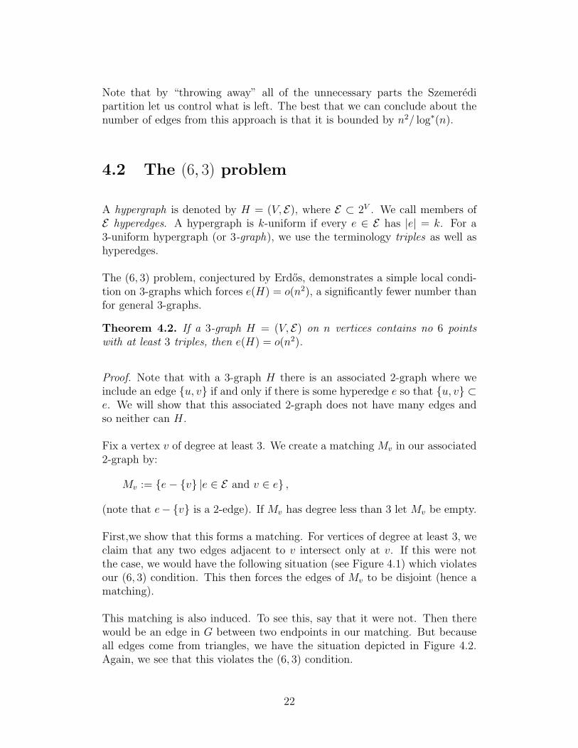
First,we show that this forms a matching. For vertices of degree at least 3, weclaim that any two edges adjacent to v intersect only at v. If this were notthe case, we would have the following situation (see Figure 4.1) which violatesour (6, 3) condition. This then forces the edges of Mv to be disjoint (hence amatching).

This matching is also induced. To see this, say that it were not. Then therewould be an edge in G between two endpoints in our matching. But becauseall edges come from triangles, we have the situation depicted in Figure 4.2.Again, we see that this violates the (6, 3) condition.

22

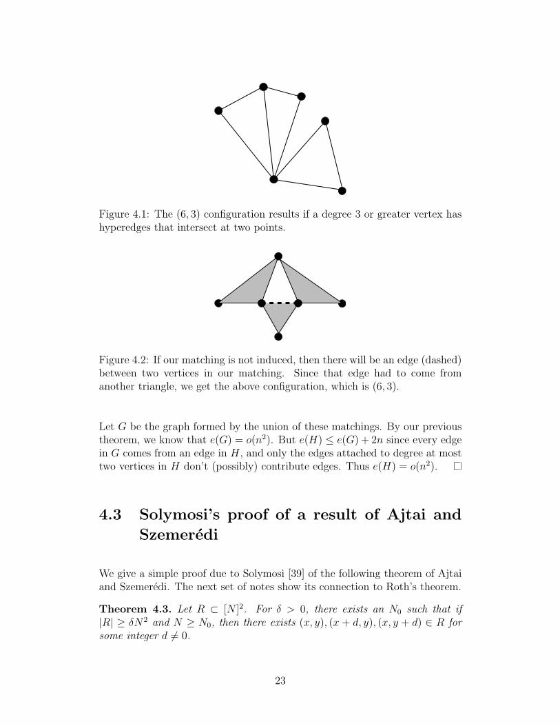
Figure 4.1: The (6, 3) configuration results if a degree 3 or greater vertex hashyperedges that intersect at two points.

Figure 4.2: If our matching is not induced, then there will be an edge (dashed)between two vertices in our matching. Since that edge had to come fromanother triangle, we get the above configuration, which is (6, 3).

Let G be the graph formed by the union of these matchings. By our previoustheorem, we know that e(G) = o(n2). But e(H) ≤ e(G) + 2n since every edgein G comes from an edge in H, and only the edges attached to degree at mosttwo vertices in H don’t (possibly) contribute edges. Thus e(H) = o(n2).

4.3 Solymosi’s proof of a result of Ajtai and

Szemeredi

We give a simple proof due to Solymosi [39] of the following theorem of Ajtaiand Szemeredi. The next set of notes show its connection to Roth’s theorem.

Theorem 4.3. Let R ⊂ [N ]2. For δ > 0, there exists an N0 such that if|R| ≥ δN2 and N ≥ N0, then there exists (x, y), (x + d, y), (x, y + d) ∈ R forsome integer d 6= 0.

23

(1,6)

(3,5)

(3,2) (6,2)

(4,3)(2,3)

(2,1)

(4,4)

(6,5)

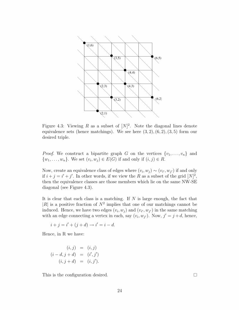
Figure 4.3: Viewing R as a subset of [N ]2. Note the diagonal lines denoteequivalence sets (hence matchings). We see here (3, 2), (6, 2), (3, 5) form ourdesired triple.

Proof. We construct a bipartite graph G on the vertices v1, . . . , vn andw1, . . . , wn. We set (vi, wj) ∈ E(G) if and only if (i, j) ∈ R.

Now, create an equivalence class of edges where (vi, wj) ∼ (vi′ , wj′) if and onlyif i + j = i′ + j′. In other words, if we view the R as a subset of the grid [N ]2,then the equivalence classes are those members which lie on the same NW-SEdiagonal (see Figure 4.3).

It is clear that each class is a matching. If N is large enough, the fact that|R| is a positive fraction of N2 implies that one of our matchings cannot beinduced. Hence, we have two edges (vi, wj) and (vi′ , wj′) in the same matchingwith an edge connecting a vertex in each, say (vi, wj′). Now, j′ = j +d, hence,

i + j = i′ + (j + d) → i′ = i− d.

Hence, in R we have:

(i, j) = (i, j)

(i− d, j + d) = (i′, j′)

(i, j + d) = (i, j′).

This is the configuration desired.

24

Lecture 5

More Applications of theRegularity LemmaD. Jacob Wildstrom

5.1 More Szemeredi Regularity Lemma Ap-

plications

5.1.1 Nonintersecting triangles

Theorem 5.1. Given a graph G with n vertices, if each edge of G lies in aunique triangle (i.e., there are no edges which lie in 2 or more distinct K3

subgraphs of G), then e(G) = o(n2).

Exercise 5.1. Prove Theorem 5.1.

5.1.2 3-Term Arithmetic Progressions

Theorem 5.2 (Roth’s Theorem [36]). For every δ > 0 there is an N(δ)so that for all n > N(δ) then if A ⊆ [n] with |A| > δn, A contains 3 terms inarithmetic progression.

Proof. We will make use of a result of Ajtai and Szemeredi (Theorem 4.3 fromthe previous lecture).

25

Let us define R ⊆ [n]2 as follows: (x, y) ∈ R if x − y ∈ A. Note that theelements of A correspond to the diagonals in the lower-left of R and so eachelement of A corresponds to between 1 and n elements of R. Even minimizingthe number of elements in R, we get that |R| > 1

2(δn)2 = εn2. Thus, by the

Ajtai-Szemeredi result using ε = 12δ2, we know that for sufficiently large n that

R contains a set of three points (x, y), (x + d, y) and (x, y + d). Since thesepoints are in R, it follows that x − y − d, x − y and x + d − y are in A, andthese three elements form an arithmetic progression of length three in A.

By now, we’ve seen several o(n) and o(n2) upper bounds on system sizes, butwhat about lower bounds? For most of these problems, we have the quite goodlower bound of n2

ec√

log n , which exceeds n2−ε for all positive ε.

We shall construct such a lower bound for the previous question.

Theorem 5.3 (Behrend’s Theorem [3]). Let r3(n) be the maximum size ofa subset of [n] not containing a 3-term arithmetic progression. Then r3(n) >

nec√

log n .

Proof. We will construct such a system based on parameters m and d whichwe shall determine later. Let us consider a set A ⊆ 0, 1, . . . ,m−1d, with anaddition operation defined termwise. There is no 3-term arithmetic progressionin A if there is no solution to the equation x + y = 2z for x, y, z ∈ A.

For a fixed t let At = (x1, x2, . . . , xd) : x21 +x2

2 + · · ·+x2d = t, so At consists of

the non-negative integer coordinates on the surface of a d-dimensional sphereof radius t. Note that every element of 0, 1, . . . ,m − 1d lies in some At for0 ≤ t ≤ m2d, so some At contains at least md/m2d = md−2/d elements. Fromgeometry we know that no three points on a sphere are colinear, so At has nothree-term arithmetic progression.

Lastly, let φ : At → Z be given by φ(x) =∑d

i=1 xi(2m)i−1; essentially, φ(x) isthe representation of x as a digit-string base 2m, so φ(At) ⊆ 0, . . . , (2m)d.From the consideration of φ(x) as a digit-string, it is clear that φ(x) + φ(y) =2φ(z) implies that x+y = 2z, from which it follows that φ(At) does not containa 3-term arithmetic progression since At does not.

By construction φ(At) is a set of size md−2/d without a 3-term arithmeticprogression drawn from a set of (2m)d consecutive integers; our lower boundis thus attained by maximizing md−2/d subject to the constraint (2m)d = n,

26

which we may rewrite as ln m = ln nd− ln 2. So we seek to maximize

ln

(md−2

d

)= (d− 2)

(ln n

d− ln 2

)− ln d

whose derivative with respect to d is

2 ln n− d− d2 ln 2

d2,

so the maximizing value of d is a solution to the quadratic d2 ln 2+d−2 ln n = 0.An approximate solution (and thus an approximate maximization) is d =√

2 log nlog 2

=√

2 log2 n. Then m = n1d /2, so

md−2

d=

nd−2

d

2d−2d= n1− 2

n− log d

log n− (d−2) log 2

log n ,

which, for vary large n, can be bounded by n1− 2

√2 log 2+ε√log n for arbitrarily small

ε.

5.2 Regularity Generalized

Our bounds on sizes of sets avoiding three-term arithmetic progresion reliedessentially on properties concerning pairs; a similar bound on avoiding four-term arithmetic progressions would require properies of triples. To generalizeour results, we must generalize the Szemeredi Regularity Lemma. Doing sois not entirely straightforward. We proceed from considering graphs, that is,structures of vertices and vertex pairs, to hypergraphs, which are structures ofvertices and vertex sets; i.e. hyper-edges are correlations among any numberof vertices, instead of simply 2. We call a hypergraph k-uniform if each edgeconsists of k vertices. A graph would be considered a 2-graph. In order toextend our results on arithmetic progressions, we shall explore variations onthe Regularity Lemma for 3-graphs and beyond.

A starting point is determining how the concepts of the Regularity Lemmaextend to triples, and in so doing we immediately encounter the complexitiesadded by our attempt to generalize. For instance, ε-regularity does not havean extension which is both intuitive and useful: while we might naıvely defineit as a requirement on vertex-sets X, Y , and Z that the densities of triplesamong subsets A, B, and C differs only by ε from the overall density, this isnot a property which always resembles randomness.

27

As an example, if we construct a random 2-graph G and induce the 3-graphH to have as edges all triples among which there are an even number of 2-edges in G (or alternatively among which there are 0 or 1 edges in G), weget hypergraphs with distributions unlike a random hypergraph generated byincluding or excluding each triple with a particular probability. We seek aproperty of graphs which will be true for a wide variety of random-hypergraphgeneration methods.

28

Lecture 6

Regularity Lemma forHypergraphsSteven Butler

In the previous lecture we saw how to use results from the regularity lemma toshow that given δ > 0 then for n sufficiently large any subset of [n] containingat least δn elements has an arithmetic progression of length 3. To show asimilar result holds for arithmetic progressions of length 4 we will need togeneralize our methods to hypergraphs.

6.1 Hypergraphs

A hypergraph H = (V, E) is is composed of V , a vertex set which is a collectionof elements, and E which corresponds to our “edges”. In a hypergraph, edgesare subsets of the vertices. In this lecture our focus will be on 3-uniformhypergraphs (which we will sometimes denote as 3-graphs) in which all theedges are subsets of order 3, i.e.,

E ⊆x, y, z : x, y, z ∈ V and x, y, z distinct

.

The graphs that we were introduced to in Section 1.2 would correspond to2-graphs.

The hardest part of working with hypergraphs is developing an intuition aboutthem. Our approach will be to define through analogy the terms which wereused in the Regularity Lemma for 2-graphs, if done properly then our proof for

29

the 2-case will apply to the more general case with hypergraphs with minimalchange. We note that our approach is based on the work of Chung [13].

6.2 Density in Hypergraphs

In Section 2.1 we defined the edge density between two subsets of vertices.Because of the added structure in a hypergraph we have more flexibility inhow to define density and we will examine two definitions of density for the3-graphs.

6.2.1 (3, 1) Density in Hypergraphs

Suppose that X, Y, Z ⊆ V then we will let eH(X, Y, Z) denote the number ofedges spanned by X,Y, Z, that is

eH(X, Y, Z) =∣∣(x, y, z) : x, y, z ∈ E(H), x ∈ X, y ∈ Y, z ∈ Z

∣∣.Note that by this convention if there is any triple (i.e., “edge” in our 3-graph)with vertices lying in X ∩ Y ∩ Z that this will get counted 6 times.

Intuitively, the edge density should be the ratio of the number of edges presentto the total number of edges possible. So let K denote the complete 3-graph(i.e., it has every possible triple in the graph). In the case X, Y, Z are alldisjoint then eK(X, Y, Z) = |X||Y ||Z|. We now define the density

δ3,1(X,Y, Z) =eH(X, Y, Z)

eK(X, Y, Z).

the 3, 1 in the subscript tells us that we are working with 3-graphs and we arelooking at the density from the 1-“dimensional” structure of the hypergraph(i.e., the density from the vertices).

With a definition of density we can now define what it means to be ε-regular.In Section 2.1 we considered subsets A ⊆ X and B ⊆ Y so that |A| ≥ ε|X|and |B| ≥ ε|Y |. But looking through the material that followed the only timewe used this condition was when we had |A||B| ≥ ε2|X||Y |, so we could haveused this as the definition and then only have been off by an ε. This will beour approach for hypergraphs.

Definition 6.1. Given X,Y, Z ⊆ V . We say that (X, Y, Z) is (3, 1)-ε-regularif for all A ⊆ X, B ⊆ Y, C ⊆ Z for which

eK(A, B, C) ≥ εeK(X, Y, Z),

30

satisfies

|δ3,1(A, B, C)− δ3,1(X, Y, Z)| < ε.

6.2.2 (3, 2) Density in Hypergraphs

If (3, 1) density used the one dimensional vertices then intuitively we wouldwant (3, 2) to use the two dimensional edges (i.e., 2-graphs) to define density.That is previously we used the natural intuition of induced triples on a vertexset (1 element subsets of V ) and now we want to think about induced tripleson pairs (2 element subsets of V ).

So given G1, G2, G3 (not necessarily disjoint) which are a set of 2-graphs onV then we will let eH(G1, G2, G3) denote the number of edges induced byG1, G2, G3 and define it as follows,

eH(G1, G2, G3) =∣∣(x, y, z) : x, y, z ∈ E(H),

x, y ∈ G1, y, z ∈ G2, z, x ∈ G3∣∣.

To count density we again want to consider the ratio of number of edges presentover the number of edges possible. Again letting K denote the complete 3-graph let

eK(G1, G2, G3) =∣∣(x, y, z) : x, y, z ∈ E(K),

x, y ∈ G1, y, z ∈ G2, z, x ∈ G3∣∣.

Then we will define our (3, 2) density by

δ3,2(G1, G2, G3) =eH(G1, G2, G3)

eK(G1, G2, G3).

This leads to the definition of being (3, 2)-ε-regular.

Definition 6.2. Given the 2-graphs G1, G2, G3. We say that (G1, G2, G3) is(3, 2)-ε-regular if for all T1 ⊆ G1, T2 ⊆ G2, T3 ⊆ G3 for which

eK(T1, T2, T3) ≥ εeK(G1, G2, G3),

satisfies

|δ3,2(T1, T2, T3)− δ3,2(G1, G2, G3)| < ε.

31

6.2.3 Comparing (3, 1) with (3, 2)

While the definitions for (3, 1)-ε-regular and (3, 2)-ε-regular are very similar toeach other we note that a special case of (3, 2)-ε-regular gives (3, 1)-ε-regular,as shown in the following exercise.

Exercise 6.1. Show that for a given graph G, (X, Y, Z) is (3, 1)-ε-regular ifand only if (X × Y, Y × Z,Z × X) is (3, 2)-ε-regular. Where by X × Y wemean the complete bipartite 2-graph which joining vertices of X to all verticesof Y .

It is possible for a graph to be ε-regular in the (3, 1) sense but not ε-regular inthe (3, 2) sense. To see this, let G be a random 2-graph with the probabilityof including an edge as 1/2, and construct a 3-graph, H, by including a triplein H if and only if 0 or 2 of the possible 2-subsets of the triple are in G.

Exercise 6.2. Show that the graph H constructed as above is ε-regular inthe (3, 1) sense, i.e., show that every triple is in H with probability of 1/2.Then show that this graph is not ε-regular in the (3, 2) sense. (Hint: letG1 = G2 = G3 = G when considering the (3, 2) case.)

6.2.4 Generalization to k-graphs

The move from (3, 1) to (3, 2) is a big leap. Once we get used to it thedefinitions will come very naturally and everything will fall into place.

For k-graphs we can similarly construct a chain of different measures of density,namely we can talk about a k-graph as being (k, r)-ε-regular for any value1 ≤ r ≤ k − 1. Generally speaking these different measure of ε-regularity arenot equivalent and the higher the value of r the “stronger” the measure ofε-regularity.

The different measures of ε-regularity give a grading to our space. This allowsone to use the language of homology when talking about the Regularity Lemmafor k-graphs. For our purposes now we will be satisfied with 3-graphs.

32

6.3 Regularity Lemma for Hypergraphs

By[

Vk

]we mean the collection of all k-subsets of V . As a special case,

[V2

]will denote the collection of all 2-subsets, or edges in a complete 2-graph.

Definition 6.3. Given H = (V, E), we say that a partition P of[

V2

]is (3, 2)-

ε-regular if∑Xi,Xj ,Xk∈P

not regular

eK(Xi,Xj,Xk) < εeK

([V

2

],

[V

2

],

[V

2

]).

That is, we want the irregular part to be small. Note we use X to emphasizethat we are working with a partition of edges and not of vertices. If we wantedto talk about a partition being (3, 1)-ε-regular we would use partitions of

[V1

],

and modify the rest of the definition similarly.

With this definition in hand we are ready to state the Regularity Lemma forhypergraphs, which is a direct analog of Theorem 3.1 in Lecture 3.

Theorem 6.1 (Regularity Lemma for Hypergraphs). Given ε > 0 andB > 1. Then for a 3-graph H with a partition P of

[V2

]where |P | ≤ B, there

is a refinement Q of P with is (3, 2)-ε-regular and |Q| is bounded above by aconstant depending only on ε and B.

The proof is analogous to that done for the Regularity Lemma for 2-graphs.Since we have introduced terminology in a way that directly corresponds to2-graphs our proof will only be a short outline. The details of any omittedstep can be found by examining the proof in Sections 3.3 and 3.4 by insertingthe proper language.

First for a given partition P of the edge sets X ,Y ,Z we define the index at(X ,Y ,Z) by

I(P (X ,Y ,Z)) =∑Xi⊆XYj⊆YZk⊆Z

eK(Xi,Yj,Zk)

eK(X ,Y ,Z)

(δ3,2(Xi,Yj,Zk)

)2,

we then define I(P ) := I(P ([

V2

],[

V2

],[

V2

])) so that

I(P ) =∑

Xi,YjZk⊆[

V2

] eK(Xi,Yj,Zk)

eK([

V2

],[

V2

],[

V2

])

(δ3,2(Xi,Yj,Zk)

)2.

33

Note that the first term (eK(Xi,Yj,Zk)/eK([

V2

],[

V2

],[

V2

])) is the portion of

the edges and sums to 1. The second term is the density, since that term issquared we see that we are in a perfect position to apply Cauchy-Schwarz,doing so gives us the following.

Fact 6.1. If P ′ is a refinement of P then I(P ′) ≥ I(P ).

We also have the following facts.

Fact 6.2. If (X ,Y ,Z) is not (3, 2)-ε-regular then there is a refinement P ′

(achieved by subdividing X ,Y ,Z into two pieces each) such that

I(P ′(X ,Y ,Z)) ≥ I(P (X ,Y ,Z)) + ε3 = δ3,2(X ,Y ,Z) + ε3.

Note when comparing this fact to the form given for the 2-graph version wesee that the ε is now cubed instead of being raised to the fourth power. Thedifference is in how we defined ε-regular, as alluded to earlier.

Fact 6.3. If the partition P is just one block then I(P ) = δ23,2. Alternatively,

if the partition P is the individual edges then I(P ) = δ3,2.

With these facts the proof of the hypergraph version of the Regularity Lemmaproceeds as before. Namely we start with our partition of edges, if it is (3, 2)-ε-regular then we are done, otherwise using our Fact 6.2 we partition each of thetriples of edge sets which are not (3, 2)-ε-regular and then repeat. Because ateach stage we will increase the index by at least ε4 then we can perform at most(δ3,2 − δ2

3,2)/ε4 refinements before having a (3, 2)-ε-regular partition. Finally

we can count the maximum elements in the resultant partition by checking ateach stage how much we have subdivided the elements. Giving us a tower of2’s similar to what we had before.

34

Lecture 7

Results on SumsetsLei Wu

This lecture was given by our guest lecturer Van Vu.

In this lecture, we will discuss many well-known results on sumsets.

7.1 Direct Problems

Definition 7.1. Let A be a finite set of integers, define the 2-fold sumsetA + A = a + a′|a, a′ ∈ A.

Intuitively, we want to say that if the set has “nice” structure, then the sumsetshould be small:

Example 7.1. Let A = 1, . . . , n, then A + A = 2, . . . , 2n. Also, one cantake an arithmetic progression instead of an interval as set A, and still obtaina small sumset (see Theorem 7.5). If A ⊆ 1, . . . , n and |A| ≥ δn, thenA + A ⊆ 2, . . . , 2n and trivially we will have

|A + A| < 2n ≤ 2

δ|A|.

In fact, one can extend this observation to the d-dimensional case. For ex-ample, consider A ⊆ Zd, A ⊆ Q, where Q is a d-dimensional integer paral-lelepiped, then we have similar results as above. Now what if we consider

35

mapping the parallelepiped to a line? The result is what we consider as thegeneralized arithmetic progression.

Definition 7.2. Let a, q1, . . . , qd be elements of an abelian group G, and letl1, . . . , ld be positive integers. The set

Q = Q(a; q1, . . . , qd; l1, . . . , ld)

= a + x1q1 + · · ·+ xdqd : 0 ≤ xi < li for i = 1, . . . , d

is called a d-dimensional (Generalized) Arithmetic Progression (GAP for short)in the group G. The length of Q is l(Q) = l1 · · · ld. Clearly, |Q| ≤ l(Q), and Qis called proper if |Q| = l(Q).

We can see that if the map from a d dimensional lattice to 1 dimension is one-to-one, then the GAP is proper. And this map is called Freiman isomorphism.

7.2 Inverse Problems

Now we consider problems in the other direction, namely, if we know theproperties of sumset A + A, can we deduce anything about the structure ofA? This is what we call the “inverse problem”.

Theorem 7.1 (Freiman). Let A be a finite set of integers such that |A+A| ≤c|A|. Then A is a large subset of some d-dimensional arithmetic progressions,i.e. there exist integers a, q1, . . . , qd, l1, . . . , ld such that

A ⊆ Q = a + x1q1 + · · ·+ xdqd : 0 ≤ xi < li for i = 1, . . . , d,

where |Q| ≤ δ|A|, and d and δ depend only on c.

A generalization of this proof is given by Ruzsa.

Theorem 7.2 (Ruzsa). Let c, c1, c2 be positive real numbers and n ≥ 1. If Aand B are finite subsets of a torsion-free abelian group such that

c1n ≤ |A|, |B| ≤ c2n

and|A + B| ≤ cn,

then A is a subset of a d-dimensional arithmetic progression of length at mostl, where d and l depend only on c, c1, and c2.

36

In fact, it was later proved that the GAP containing A can be made proper(e.g., see Chang [8] and Bilu [5]). Chang also improved the bounds of thedependency on c in Freiman’s Theorem, namely to

d(c) ≤ bc− 1c, δ(c) ≤ expKc2(ln c)3,

where K is an absolute constant.

Bilu[5] also gave a proof of Freiman’s Theorem, which is close to Freiman’sproof and has more combinatorial flavor.

Theorem 7.3. Let A ⊆ Z and |A+A| ≤ c|A|, then there exists a d-dimensionalarithmetic progression Q such that

d = blog2 cc,

and A′ ⊆ A such that

|A′| ≥ α|A|, A′ ⊆ Q,

and

|A′| ≥ δ|Q|,

where α = α(c) and δ = δ(c) = exp− exp(c).

7.3 Balog-Szemeredi

Suppose we only have partial information about the sumset, say, if a “largeportion” of it is “under controll”, then we can still deduce information abouta large subset of the original set.

Theorem 7.4 (Balog-Szemeredi). Suppose A is a subset of a finite abeliangroup with |A| = n, and G is a bipartite graph with color classes A and A, and

|E(G)| ≥ εn2.

Let A +G A = a + a′|(a, a′) ∈ E(G), and assume

|A +G A| ≤ c|A|,

then there exists a set A′ ⊆ A such that

|A′| ≥ α|A|,

and

|A′ + A′| ≤ k|A′|,

where α = α(c, ε) and k = k(c, ε).

37

The original proof of this theorem used the Regularity Lemma, hence thebound is a tower function in c. Tim Gowers improved this bound by obtaininga polynomial function in c in his proof of Szemeredi’s Theorem for arithmeticprogression of length 4. Just as the generalization of Freiman’s Theorem byRuzsa, this theorem could also be generalized to the case when we take twodifferent sets A and B of roughly the same size. An open problem is that if |A|is significantly smaller than |B|, say |A| = n1/3 and |B| = n, |A +G B| ≤ c|B|,and |E(G)| ≥ εn4/3, then what can we say about the structure of (a largesubset of) A and B?

7.4 Cauchy-Davenport

There are also a few problems concerning sumsets in congruence classes. First,recall two well-known theorems:

Theorem 7.5. Let A ⊂ Z, and |A| = n. Then

|A + A| ≥ 2n− 1,

and equality holds if and only if A is an arithmetic progression.

Theorem 7.6 (Cauchy-Davenport). Let p be a prime number, and A, Bbe nonempty subsets of Zp, then

|A + B| ≥ minp, |A|+ |B| − 1.

Similar questions can be raised on distinct sumsets.

Definition 7.3. Let A ⊆ Z, define distinct 2-fold sumset

A∗+ A = a + a′|a, a′ ∈ A, a 6= a′.

And we have the following counterparts of Theorem 7.5 and Theorem 7.6.

Theorem 7.7. Let A be defined as in Theorem 7.5, then

|A∗+ A| ≥ 2n− 3,

and equality holds if and only if A is an arithmetic progression.

Theorem 7.8 (Erdos-Heilbronn Conjecture). Let A be as in Theorem7.6, then

|A∗+ A| ≥ min2n− 3, p.

38

This conjecture was proved in the 90’s by Dias da Silva and Hamidoune usingrepresentation theory and linear algebra, and later by Alon, Nathanson andRuzsa through polynomial methods.

Note that all the problems in this section can be generalized to h-fold sumsetsfor all h ≥ 2.

39

Lecture 8

Quasi-Random HypergraphsPaul Horn

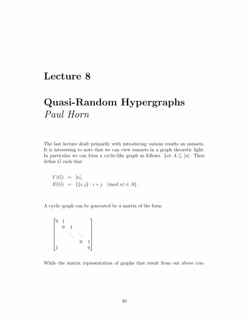
The last lecture dealt primarily with introducing various results on sumsets.It is interesting to note that we can view sumsets in a graph theoretic light.In particular we can form a cyclic-like graph as follows. Let A ⊆ [n]. Thendefine G such that

V (G) = [n],

E(G) = i, j : i + j (mod n) ∈ A.

A cyclic graph can be generated by a matrix of the form

0 1

0 1. . .

. . .

0 11 0

While the matrix representation of graphs that result from our above con-

40

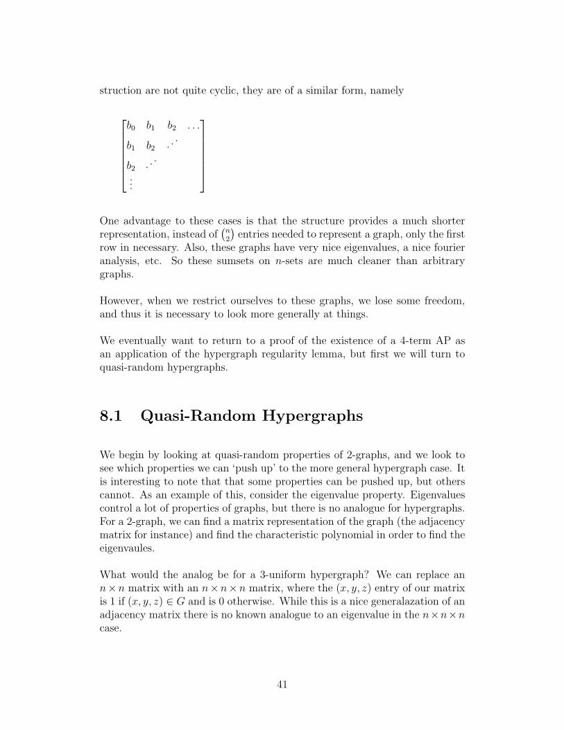
struction are not quite cyclic, they are of a similar form, namely

b0 b1 b2 . . .

b1 b2 . ..

b2 . ..

...

One advantage to these cases is that the structure provides a much shorterrepresentation, instead of

(n2

)entries needed to represent a graph, only the first

row in necessary. Also, these graphs have very nice eigenvalues, a nice fourieranalysis, etc. So these sumsets on n-sets are much cleaner than arbitrarygraphs.

However, when we restrict ourselves to these graphs, we lose some freedom,and thus it is necessary to look more generally at things.

We eventually want to return to a proof of the existence of a 4-term AP asan application of the hypergraph regularity lemma, but first we will turn toquasi-random hypergraphs.

8.1 Quasi-Random Hypergraphs

We begin by looking at quasi-random properties of 2-graphs, and we look tosee which properties we can ‘push up’ to the more general hypergraph case. Itis interesting to note that that some properties can be pushed up, but otherscannot. As an example of this, consider the eigenvalue property. Eigenvaluescontrol a lot of properties of graphs, but there is no analogue for hypergraphs.For a 2-graph, we can find a matrix representation of the graph (the adjacencymatrix for instance) and find the characteristic polynomial in order to find theeigenvaules.

What would the analog be for a 3-uniform hypergraph? We can replace ann×n matrix with an n×n×n matrix, where the (x, y, z) entry of our matrixis 1 if (x, y, z) ∈ G and is 0 otherwise. While this is a nice generalazation of anadjacency matrix there is no known analogue to an eigenvalue in the n×n×ncase.

41

8.1.1 Properties of Quasi-Random Graphs

It is important to understand that the ‘quasi-random’ properties that we lookat are not random at all, in fact they are completely deterministic. They are,however, motivated by randomness, and can be thought of as a measure of howrandom a particular graph is. Quasi-randomness is not a phenomenon thatis exclusive to graph theory, however. For instance Chung and Graham [12]treat the subject of quasi-random subsets and sequences.

The following are some properties of quasi-random graphs. Let G be a graphon n vertices.P1 : G has ≥ (1 + o(1))n2

4edges, and ≤ (1 + o(1))n4

16C4’s.

P2(s) (for a fixed s ≥ 4): Each graph M on S vertices occurs in (1+ o(1)) ns

2(s2)

times as an individual subgraph.P3 : For any subset S ⊆ V (G), the number of edges spanned by S is e(S) =|S|24

+ o(n2).P4 : For all but o(n2) pairs of vertices u and v, the number, s(u, v) of verticesadjacent to both u and v is s(u, v) = (1 + o(1))n

2.

P5 : If A is the adjacency matrix of G, with eigenvalues λ1 ≥ |λ2| ≥ · · · ≥ |λn|.,then

λ1 = (1 + o(1))n

2,

λ2 = o(n).

Exercise 8.1. 1.) Show that P2(s) ⇐ P2(s + 1)2.) Show that P5 ⇒ P3

3.) Show that P1 ⇒ P5.

8.1.2 Notes on Properties of Quasi-Random Graphs

It is interesting to note that we have the following relations regarding P2(S).

P2(2) ⇐ P2(3) ⇐ P2(4) ⇐ P2(5) ⇐ . . . P2(s); ; ⇒ ⇒ ⇒

One can, for instance, see that P2(2) ; P2(3) by considering G being thedisjoint union of two copies of Kn/2, which has the expected number of edges,but not the expected number of triangles.

42

With P3, note that for a small subset, the guess could be very wrong, hencethe o(n2) error term. For instance, Ramsey theorey implies that G will haveeither an independent set or a clique of size log(n). Thus this error term isnecessary for the property to be valid.

Note that for P5, we listed the eigenvalues of G as λ1 ≥ |λ2| ≥ · · · ≥ |λn|.This is a consequence of Perron and Frobenius [27], which implies that λ1, thelargest eigenvalue in absolute value, is positive. Also as noted above, sincethese are eigenvalue properties, they do not push through to the hypergraphcase.

It is also interesting to note that although these conditions have certain re-lationships (see, for instance, the Exercise 8.1) they are in some sense verydifferent. For instance, P3 is a global property, but P4 can be thought of asa neighborhood property. Also, some of the properties are more difficult tocheck than others. P2 is hard to verify, for instance, but P5 can be checkedby computing the characteristic equation, which takes polynomial time in n.Likewise, P1 can be verified in n4 steps. Thus the game is to find propertiesthat are easy to verify, and estimate others, and use the relationships betweenproperties for information on the graphs.

Finally, we note that these same properties can make sense in other configu-rations. For instance, these same basic properties make sense if we restrict tothe family of cyclic graphs, or equivalently subsets of an n set. More detailson this can be found in [14].

8.1.3 Properties for Quasi-Random Hypergraphs

We now work to see which properties can be generalized to k-graphs. Chungand Graham [15] examine this generalization.

First we note that P2(s) is easy to generalize, as we can talk about hypergraphson s vertices, and inspect a hypergraph for copies of a certain induced sub-hypergraph. Thus we can generalize it as the following k-graph property fora k-regular hypergraph on n vertices H.Q2(s) : Each k-graph M on s vertices occurs in H

(1 + o(1))ns

2(sk)

times.

We next set our sights at generalizing P3. We begin by considering the k = 3

43

case. In a previous lecture we looked at 3-regular hypergraphs induced on2-graphs. Given a 3-graph H, and a 2-graph S ⊆

[n2

]we are concerned with

looking for copies of K3 within S. We would expect that there are about12

( |S|n2

)n3

6unordered triples in the graph, where |S|

n2 is the probability that aparticular edge is in S, and the constant 1

2comes from our view that H should

look like a hypergraph with edge probability 12.

Generalizing this to a k-graph we get that the expected number of hyperedges

spanned by a (k − 1)-graph is 12

nk

k!

(|S|

nk−1

)k

, and hence we get our generalized

P3.Q3 : For any (k − 1)-graph S, the number of edges of H spanned by S is

(1 + o(1))nk

k!

(|S|

nk−1

)k

.

44

Lecture 9

Quasirandomness, RamseyGraphs, and ExplicitConstructionsRoss Richardson

We discuss graphs (specifically, graph families) with given properties, and thendiscuss the problem of explicitly describing graphs in such families.

9.1 Quasirandom Graphs

We begin by stating a few properties for a graph. We remark that theseproperties are satisfied by random graphs from G(n, 1/2). Nonetheless, thegraph properties that we describe do not depend on any input of “randomness”.For the following, let G be a graph on n vertices.

• P(s) (s fixed and at least 4): For any fixed graph M on s vertices, itsoccurrence in G is (1 + o(1)) ns

2(s2)

as a labeled induced subgraph.

• P1: G has at least (1 + o(1))n2

4edges and less than (1 + o(1))n4

16labeled

induced C4’s.

• P2: For any S ⊂ V (G), e(S) = |S|24

+ o(n2).

45

• P3: Let S(u, v) = w : (w ∼ u and w ∼ v) or (w u and w v). Foralmost all pairs |S(u, v)| = (1 + o(1))n

2.

As elaborated in the last notes, these (and other) properties are equivalent andform a family of checkable properties for a graph to be quasi-random. It ishelpful to consider examples of graph families that satisfy the above properties.First of all, it is not hard to show random graphs (or almost all graphs) arequasi-random. It is often desirable to have “explicit constructions” insteadof only existence proofs via probabilistic methods. By explicit constructions,we mean a succinct description (a polynomial algorithm, for example) for aninfinite family of graphs which satisfy the desired property (properties).

Happily, there have been such explicit constructions of quasi-random graphs.

Example 9.1 (Paley Graphs). Let p be prime. Define the graph Qp onvertices 1, . . . , p− 1 by the relation that u ∼ v if and only if u − v is aquadratic residue modulo p.

We show that this graph satisfies property P3.

We shall need two facts about quadratic residues.

Lemma 9.1. The number of quadratic residues in 0, . . . , p− 1 modulo p isp−12

.

Proof. This follows from the fact that for x, y ∈ [p− 1], x2 = y2 exactly whenp divides one of x + y or x− y. Hence, every quadratic residue corresponds totwo distinct elements of [p− 1], yielding our equality.

Lemma 9.2. For x, y ∈ [p − 1], xy

is a quadratic residue precisely when bothx and y are or neither are.

Proof. Observe that for a fixed quadratic residue x, xy

is a quadratic residue

exactly when y is. As the quotients xy

are distinct for all y ∈ [p − 1], we use

the above lemma to see that the number of xy

which are not residues is p−12

(corresponding to y a non-residue).

Thus, if x is a non-residue, we know that p−12

of the quotients xy

are non-residues, corresponding to the case when y is a residue. Thus, the remainingquotients are all residues, corresponding to the case when both x and y arenon-residues.

46

Thus, in particular, we see that Qp is a (p− 1)/2 regular graph. Further, foru, v, w ∈ V (Qp), w ∈ S(u, v) if and only if u− w and v − w are both residuesor non-residues. Hence, by our theorem w ∈ S(u, v) if and only if u−w

v−wis a

residue. Thus, we need only count the number of times the quotient u−wv−w

is aresidue for w not equal to u or v, as this will yield the size of S(u, v). As thisquotient is unique for each w, and ranges over all values except 0 and 1, wesee that |S(u, v)| = p−1

2− 1, corresponding to the obtained residues. But this

is enough to see that the family Qp satisfies P3.

We mention another construction for a quasi-random graph, which will gener-alize to the hypergraph case.

Example 9.2. Let G be a graph on 2n vertices such that V (G) =[

2nn

], that

is, subsets of size n of the set [2n]. Let U ∼ V if and only if |U ∩ V | ≡ 0(mod 2).

9.2 Ramsey Graphs

We can define r(k) to be the number of vertices required for a graph to haveeither a k clique or a k independent set. Ramsey theory gives bounds

c√

2k≤ r(k) ≤ c′4k,

for constants c and c′.

Thus, we are assured that for n large there exist graphs of with no clique ofsize c′′ log n and no independent set of size c′′ log n. We say such graphs havethe Ramsey Property. It is of interest to find explicit constructions of suchgraphs (Erdos offered $100 for such constructions). Such a construction how-ever, has been elusive. Constructions such as the Paley graph, which provideconcrete examples of many types of conditions (quasirandom, expander, etc.),fail to have this Ramsey Property. Indeed, though one can see that the Paleygraph has clique size at most c

√p, it was shown to contain cliques of size

c log p log log log p infinitely often.

The search for constructions of graphs with cliques and independent sets ofsize n1/k remains difficult. The current state of the art rests at e

√log n.

Here, we list a graph shown by Frankl and Wilson to have clique and indepen-dent size at most ec(log n log log n)1/2

(which forces r(k) > kc log k/ log log k).

Example 9.3. Let q be a prime power. The graph G will have vertex setV = F ⊂ [m] : |F | = q2 − 1 and edge set E = (F, F ′) : |F ∩ F ′| 6≡ −1

47

(mod q). This graph contains no clique of size(

mq−1

). By setting m = q3, we

find a graph on n =(

mq2−1

)vertices with no clique or independent set of the

size claimed.

The point here is that such Ramsey graphs are somehow stricter measuresof randomness than properties such as quasi-randomness, and thus it is notsurprising that explicit construction of Ramsey graphs are harder to come by.

9.3 Hypergraphs

In the last lecture, we saw how to generalize the property P(s) to hypergraphs.We note that much as in the graph case, infinitely many of these propertiesare equivalent. More precisely, for the k−uniform case, we have the followingimplications:

P(k) ⇐ P(k + 1) ⇐ . . . ⇐ P(2k) ⇐ P(2k + 1) . . .; ; ; ⇒ ⇒

One question is whether we might generalize property P1, that is, whether wemight find some hypergraph analogue for C4. The answer to our question isyes, and such a graph is as follows.

We define the k−uniform hypergraph Ok by V (Ok) = vi,j : 1 ≤ i ≤ k, 0 ≤j ≤ 1 with edges E(Ok) = v1,i1 , v2,i2 , . . . , vk,ik : i1, . . . , ik ∈ 0, 1. Whenk = 3 the resulting graph corresponds to the faces of an octahedron, hence itsname.

Property P1 is then readily generalized using this graph.

9.3.1 Quasi-random Hypergraphs

We also demonstrate two quasi-random hypergraphs. The first is a general-ization of the subset intersection graph we saw earlier.

Example 9.4 (Even Intersection Graph). Construct a k−uniform hyper-graph with vertex set V (H) = 2[n] (that is the vertices consist of all possiblesubsets of [n]). Then the subsets X1, . . . , Xk form an edge if and only if|X1 ∩ · · · ∩Xk| ≡ 0 (mod 2).

48

We may also generalize the Paley graph and obtain a quasi-random hyper-graph, as follows:

Example 9.5. For p a prime, let i1, . . . , ik be an edge if and only if i1+. . .+ikis a quadratic residue.

49

Lecture 10

Discrepancy of GraphsBlair Angle

10.1 Some Preliminary Definitions

Definition 10.1. Given a k-uniform hypergraph H = (V, E), define the indi-cator function µk :

(Vk

)→ −1, 1 by

µH(v1, v2, . . . , vk) :=

−1 if v1, v2, . . . , vk ∈ E ,1 otherwise.

Note that in this definition, we are assuming that the vi’s are distinct. We willslightly modify this definition where we now allow vi = vj for i 6= j.

Definition 10.2. Given a k-uniform hypergraph H = (V, E), we define thefunction µH : V k → −1, 1 by

µH(v1, v2, . . . , vk) :=

µH(v1, v2, . . . , vk) if the vi are all distinct,1 if vi = vj for some i 6= j.

Note that edges in H is given by µ−1H (−1) = µ −1

H (−1), and so the number ofedges is |µ−1

H (−1)|.

Definition 10.3. Given a k-uniform hypergraph H = (V, E), let H denote thecomplement of H, the the k-uniform hypergraph with vertex set V and edgeset(

Vk

)− E(H).

50

We remind the reader of the definition of an octahedron.

Definition 10.4. An octahedron, O2k, is a k-hypergraph with vertex set V =vεi

i : 1 ≤ i ≤ k, εi = 0, 1 and edge set E =vε1

1 , . . . , vεkk : εi = 0 or 1

.

When k = 2, O4 is C4, the cycle on 4 vertices. The reader may want to verifymany of the facts presented in the next section of this chapter in this specialcase (i.e., k = 2) before tackling general k.

10.2 The Deviation of a Hypergraph

10.2.1 Some Facts

We now define the deviation of a hypergraph.

Definition 10.5. Given a k-uniform hypergraph H = (V, E), the deviation ofH is given by

dev H :=1

n2k

∑1≤i≤k

v0i

,v1i∈V

∏εj∈0,11≤j≤k

µH

(vε1

1 , . . . , vεkk

).

Given a set of 2k vertices we have that a term in the sum above is 1 if aneven number of edges in O2k is in H and gives −1 if an odd number of edgesin O2k is in H. So another way to calculate dev H is to take the number of“even octahedron” then take away the number of “odd octahedron”, take theresulting value and divide by n2k.

While the formula for deviation is somewhat ugly, its redeeming property isthat it is straightforward to compute. One application of the deviation functionis given by the following theorem:

Theorem 10.1. Given a k-uniform hypergraph H(n) on n vertices, for anyfixed G(t) (a k-hypergraph on t vertices), a bound on the number of labelledoccurrences of G(t) in H(n) is given by:∣∣∣∣∣#G(t) < H(n) − nn(n−1)···(n−t+1)

2(tk)

∣∣∣∣∣ ≤ 5nt(devH(n))2−k

.

Now we present several facts about the deviation of a k-uniform hypergraphH.

51

Fact 10.1. dev H = dev H.

This follows immediately from the definition of deviation. Since an edge isin H if and only if it is not in H. In changing from dev H to dev H we areflipping 2k signs and so overall nothing changes (i.e, each term in the sum is aproduct of 2k values which go from 1 to -1, or go from -1 to 1). Another wayto see this is to note that the number of faces in O2k is even.

Fact 10.2. 0 ≤ dev H ≤ 1.

There are exactly n2k ordered 2k-tuples of the vertices of H (allowing repeats).So clearly∣∣∣∣∣ ∑

1≤i≤k

v0i

,v1i∈V

∏εj∈0,11≤j≤k

µH

(vε1

1 , . . . , vεkk

)∣∣∣∣∣ ≤ n2k.

So with the normalization factor of 1n2k in the definition of deviation, it is clear

that dev H ≤ 1. The other inequality is left as an exercise. One way this canbe achieved is to show that the deviation of H can be expressed as

1

n2k

∑1≤i≤k−1

v0i

,v1i∈V

(∑w∈V

∏ε1,...,εk−1

µH

(vε1

1 , . . . , vεk−1

k−1 , w))2

.

(Note: in deriving this expression, the reader may want to first start with thesimplest octahedron, C4.)

The neighborhood of a vertex in a k-hypergraph is a (k−1)-hypergraph. Givenany vertex in a k-hypergraph H, define

H(v) := the neighborhood of v.

Definition 10.6. The sameness graph of u and v denoted by H(u)∇H(v) isa (k − 1)-hypergraph with vertex set H(u) ∪ H(v) where e is an edge of thesameness graph if and only if e is either in both of H(u) and H(v), or e is inneither.

This leads us to our next fact:

Fact 10.3.

dev H =1

n2

∑u,v∈V

dev(H(u)∇H(v)

).

52

This is done by using the definition of deviation and the observation thatµ

H∇H′= −µ

Hµ

H′.

Definition 10.7. Given any 2-graphs G and H, the Cartesian Product G His the 2-graph with vertex set V (G) × V (H) and (u, v) ∼ (a, b) if and only ifu = a and v ∼ b in H, or v = b and u ∼ a in G.

Note there are several ways to define the product of a graph, you only need todetermine what happens on the four cases of (edge/no edge)×(edge/no edge).The advantage of the definition above is that it makes grids which simulatemultidimensional space.

Fact 10.4. dev G H = (dev G)(dev H).

The proof of this is left as an exercise.

We can define the Cartesian product of 3-graphs similarly. That is we havevertex set V (G)× V (H) and (u1, v1), (u2, v2), (u3, v3) is an edge if and onlyifu1 = u2 = u3 and v1, v2, v3 ∈ E(H)

orv1 = v2 = v3 and u1, u2, u3 ∈

E(G).

10.2.2 Deviation and Discrepancy

A quantity related to discrepancy is deviation, which though deviation has anicer looking formula, it is actually more difficult to compute than the devia-tion. In the next chapter, we will look at relationships between the deviationand discrepancy. We will prove the following theorem:

Theorem 10.2. For any k-hypergraph H, discH ≤ (dev H)2−kand dev H ≤

4k(disc H)2−k.

53

Lecture 11

Relating Deviation andDiscrepancy for Hypergraphs,Part 1Kevin Costello

11.1 Deviation

Let H be a k-regular hypergraph on n vertices (with k small relative ton). Equivalently, we can think of H as a function µ = µ

Hfrom the

(nk

)different k-element subsets of the vertex set V to the set 1,−1, whereµ

H(v1, v2, . . . , vk) = 1 if and only if v1, . . . , vk is not an edge of H. We

can extend µ to a function µ on all ordered k-tuples of vertices by definingµ(v1, . . . , vk) to be 1 if any two of v1, . . . , vk are equal.

We define the deviation of H to be

1

n2k

∑v0i

,v1i

i=1,...,k

∏εi∈0,1i=1,...,k

µ(vε11 , . . . , vεk

k ).

11.2 Discrepancy

Let H be a k-regular hypergraph and G a (k − 1)-regular hypergraph on thesame set of vertices. Define E(H; G) to be those edges in H “induced” by G,

54

that is all edges in H such that dropping any vertex gives an edge of G. Forexample, in a standard simplex every element of the k-skeleton is induced bythe (k − 1)-skeleton. Let e(H; G) = k!|E(H; G)| be the number of (labelled)k−edges in H induced from G.

We define the discrepancy on H to be

1

nkmax

G|e(H; G)− e(H; G)|,

where the maximum is taken over all (k − 1)-graphs on the vertex set of H.Here we are assuming that H has edge density approximately 1/2, so we expecte(H; G) and e(H; G) to be roughly equal.

If we take G to be the complete (k − 1)−graph on the vertices of H, we getthat the discrepancy is bounded below by 2|δ(H) − 1/2| (where δ(H) is theedge density of H). Similarly, we can use the discrepancy to get a bound onthe edge density of any large subset of the vertex set.

Although the discrepancy of H has many useful properties, it is difficult tocompute since there are many possible choices for G. Our eventual goal is torelate the discrepancy to the (more computable) deviation. Specifically, weaim to show that for any H, disc H ≤ (dev H)2−k

and dev H ≤ 4k(disc H)2−k.

A corollary to this result is that if either the deviation or the discrepancy ofH is o(1), the other must be o(1) as well.

11.3 The l-deviation of a Graph and its prop-

erties

Define the l-deviation of H as follows:

devl H =1

nk+l

∑v0i

,v1i

i=1,...,l

∑vj

j=l+1,...,k

∏ε1,...,εlεi∈0,1

µ(vε11 , . . . , vεl

l , vl+1, . . . , vk).

Note that we have devk H = dev H and dev0 H = 1nk e(V, V, . . . , V ) = δ(H).

Theorem 11.1. We have devl H ≥ (devl−1 H)2. In particular, devl H, (andthus dev H) is always nonnegative.

55

Proof. First, we split up the innermost product according to whether εl = 0or εl = 1, as shown below.∏

ε1,...,εlεi∈0,1

µ(vε11 , . . . , v

εl−1

l−1 , vεll , vl=1, . . . , vk) =

(∏µ(vε1

1 , . . . , vεl−1

l−1 , v0l , vl+1, . . . , vk)

)×(∏

µ(vε11 , . . . , v

εl−1

l−1 , v1l , vl+1, . . . , vk)

)Using this we can rewrite our sum for devl H as∑

v0i

,v1i

i=1,...,l−1

∑vj

j=l+1,...,k

(∑v0

l

∑v1

l

( ∏µ(vε1

1 , . . . , vεl−1

l−1 , v0l , vl+1, . . . , vk)×∏

µ(vε11 , . . . , v

εl−1

l , v1l , vl+1, . . . , vk)

)).

The innermost two sums are independent and we can factor according to

n∑i=1

m∑j=1

aibj = (n∑

i=1

ai)(m∑

j=1

bj).

The two terms in the product of the right side of this identity correspond totaking εl = 0 and εl = 1, which are equal by symmetry. Thus we are left with:∑

v0i

,v1i

i=1,...,l−1

∑vj

j=l+1,...,k

(∑vl

( ∏ε1,...,εl−1εi∈0,1

µ(vε11 , . . . , v

εl−1

l−1 , vl, vl+1, . . . , vk)))2

.

We now apply the Cauchy-Schwartz inequality (∑m

i=1 a2i ≥ (

∑mi=1 ai)

2/m) withaj equal to the innermost sum in the above expression. Here m is equal to thenumber of summands, n2(l−1)+(k−l). Doing so gives us that

devl H ≥

( ∑v0i

,v1i

i=1,...,l−1

∑vj

j=l,...,k

∏ε1,...,εl−1εi∈0,1

µ(vε11 , . . . , v

εl−1

l−1 , vl, . . . , vk)

)2

nk+ln2(l−1)+(k−1)

=(nk+l−1devl−1 H)2

nk+l+2(l−1)+(k−l)= (devl−1 H)2.

56

Lecture 12

Relating Deviation andDiscrepancy for Hypergraphs,Part 2Daniel Felix

12.1 Discrepancy and Deviation

Let H = (V, µH) be a k-uniform hypergraph. Recall the following two defini-

tions.

Definition 12.1. The discrepancy of H is defined as

disc H = n−k maxG

(k−1)−graph

|e(H; G)− e(H; G)|.

It is understood that each of the (k−1)-uniform hypergraphs satisfies V (G) ⊂V . By convention, no edge of G contains a repeated vertex.

Definition 12.2. The deviation of H is defined as

dev H = n−2k∑

vi(0),vi(1)1≤i≤k

∏εj∈0,11≤j≤k

µH(v1(ε1), . . . , vk(εk)).

(In previous lectures we wrote this as (vε11 , . . . , vεk

k ).) We will usually expressthis more compactly as

dev H = n−2k∑

~v

∏~ε

µH(~v(~ε)), (12.1)

57

where the sum is taken over all ~v = (v1(0), v1(1), . . . , vk(0), vk(1)) in V 2k andthe product is taken over all ~ε ∈ 0, 1k.

We will show that these two quantities are closely related, and that one canbe small only if the other is as well. We state this more precisely as a theorem.

12.2 Connection Between Discrepancy and De-

viation

Theorem 12.1. For any k-graph H = (V, µH), the following inequalities al-

ways hold:

(i) disc H ≤ (dev H)2−k

,

(ii) dev H ≤ 4k(disc H)2−k

.

This is theorem 8.1 in [12], which gives a thorough treatment of many aspectsof deviation.

We will only prove the first inequality in this lecture, and before doing so itwill be convenient to introduce some notation. We will use ~v(i) to denote thevector in which the vi(0) and vi(1) coordinates have been removed from ~v:

vi(i) = (v1(0), v1(1), . . . , vi−1(0), vi−1(1), vi+1(0), vi+1(1), . . . , vk(0), vk(1)).

Similarly, ~ε(i) will denote the vector

(ε1, . . . , εi−1, εi+1, . . . , εk).

We let ~v(~ε(i); u) denote the vector acquired by removing the ith entry of ~v(~ε)and replacing it with the vertex u. That is,

~v(~ε(i); u) = (v1(ε1), . . . , vi−1(εi−1), u, vi+1(εi+1), . . . , vk(εk)).

Lastly, ξ(G) will denote the edge set of the hypergraph G.

Proof of (i). First consider the case k ≥ 3, and let G be a (k − 1)-uniformhypergraph with no “loops” (edges containing a repeated vertex) and which

58

satisfies V (G) ⊂ V . Notice that by definition

n2kdev H =∑

~v

∏~ε

µH(~v(~ε))

=∑~v(1)

∑v1(0),v1(1)

∏~ε(1)

µH(~v(~ε(1); v1(0)))µH(~v(~ε(1); v1(1)))

=∑~v(1)

∑u

∏~ε(1)

µH(~v(~ε(1); u))

2

≥∑

~v(1)⊂ξ(G)

∑u

∏~ε(1)

µH(~v(~ε(1); u))

2

. (12.2)

We pause here for a clarification. Clearly ~v(1) is an element of V 2k−2, whichitself is not a subset of ξ(G). When we write ~v(1) ⊂ ξ(G) we mean that theabove sum is to be taken over all vectors ~v(1) such that ~v(1)(~ε(1)) is an edgeof G for all ~ε(1) ∈ 0, 1k−1. The expression ~v(1)(~ε(1)) should be interpretedin the same way as ~v(~ε) in equation (12.1); that is,

~v(1)(~ε(1)) = (v2(ε2), . . . , vk(εk)).

By expanding the squared term of (12.2), we find that

n2kdev H ≥∑

~v~v(1)⊂ξ(G)

∏~ε

µH(~v(~ε)).

Assuming that

n2kdev H ≥∑

~v~v(i)⊂ξ(G)

1≤i≤j

∏~ε

µH(~v(~ε)),

where j is fixed, we have

n2kdev H ≥∑

~v~v(i)⊂ξ(G)

1≤i≤j

∏~ε

µH(~v(~ε))

=∑

~v(j+1)

∑vj+1(0)∈S0

∑vj+1(1)∈S1

∏~ε(j+1)l=0,1

µH(~v(~ε(j + 1); vj+1(l))). (12.3)

The sets S0 and S1 are another piece of notational shorthand. Our sum mustcontain the information that ~v(i) ⊂ ξ(G) for all 1 ≤ i ≤ j, so we use S0 andS1 to represent that the choices of vj+1(0) and vj+1(1) are restricted. If, for

59

example, no choice of vj+1(1) can be made that fulfills the requirements, thenS1 is empty. Notice that in principle S0 does depend on the previously chosenvertices v1(0), . . . , vj(1), vj+2(0), . . . , vk(1), while S1 depends on these verticesas well as vj+1(0).

Our first observation is that S1 does not actually depend on vj+1(0) becausein no choice of ~ε does the vector ~v(~ε) contain both of the vertices vj+1(0) andvj+1(1). Secondly, if u and v are valid choices for vj+1(0) and vj+1(1), thensurely we can interchange the two vertices to obtain another valid pair. HenceS0 = S1, and vj+1(0) and vj+1(1) can be chosen arbitrarily from this set. Wemay then rewrite (12.3) as follows:

n2kdev H ≥∑

~v(j+1)

∑u∈S0

∏~ε(j+1)

µH(~v(~ε(j + 1); u))

2

≥∑

~v(j+1)∈ξ(G)

∑u∈S0

∏~ε(j+1)

µH(~v(~ε(j + 1); u))

2

.

Expanding the resulting sum yields

n2kdev H ≥∑

~v~v(i)⊂ξ(G)

1≤i≤j+1

∏~ε

µH(~v(~ε)).

Therefore, by induction,

n2kdev H ≥∑

~v~v(i)⊂ξ(G)

1≤i≤k

∏~ε

µH(~v(~ε)). (12.4)

Note that we may rewrite the condition ~v(i) ⊂ ξ(G) for all i as ~v ⊂ ξ(K, G),where K denotes the complete k-uniform hypergraph on V .

The next step is to apply the Cauchy-Schwarz inequality to (12.4) k times.We prove by induction on t that

n2kdev H ≥t∏

l=1

(1

n2k−l−1

)2t−1 ( ∑u1,...,ut

∑vi(0),vi(1)

i>t~v⊂ξ(K,G)

∏εj

j>t

µH(~u,~v(~ε))

)2t

(12.5)

for all 1 ≤ t ≤ k. The expression µH(~u,~v(~ε)) is used in place of the morecumbersome

µH(u1, . . . , ut, vt+1(εt+1), . . . , vk(εk)).

60

Our intention is for the value of t in such an expression to be inferred fromthe ranges of the above sums and products.

Rewriting (12.3) yields

n2kdev H ≥∑

vi(0),vi(1)i>1

( ∑u1

~v⊂ξ(K,G)

∏εj

j>1

µH(u1, v2(ε2), . . . , vk(εk))

)2

Compare this to (12.2). The two are nearly identical; only the condition~v ⊂ ξ(K, G) separates them. We now apply a version of the Cauchy-Schwarzinequality

n∑i+1

a2i ≥

1

n

(n∑

i+1

ai

)2

to obtain that

n2kdev H ≥ 1

n2k−2

( ∑vi(0),vi(1)

i>1

∑u1

~v⊂ξ(K,G)

∏εj

j>1

µH(u1, v2(ε2), . . . , vk(εk))

)2

which is exactly (12.5) for t = 1. Now assume that (12.5) is true for t =1, . . . , t0 and consider the sum∑

u1,...,ut0

∑vi(0),vi(1)

i>t0~v⊂ξ(K,G)

∏εj

j>t0

µH(~u,~v(~ε))

=∑

u1,...,ut0

∑vi(0),vi(1)

i>t0~v⊂ξ(K,G)

∏εj

j>t0

µH(u1, . . . , ut0 , vt0+1(εt0+1), . . . , vk(εk))

=∑

u1,...,ut0

∑vi(0),vi(1)

i>t0+1

( ∑ut0+1

~v⊂ξ(K,G)

∏εj

j>t0+1

µH(u1, . . . , ut0+1, vt0+2(εt0+2), . . . , vk(εk))

)2

≥ 1

n2k−(t0+1)−1

( ∑u1,...,ut0+1

∑vi(0),vi(1)

i>t0+1~v⊂ξ(K,G)

∏εj

j>t0+1

µH(u1, . . . , ut0+1, vt0+2(εt0+2), . . . , vk(εk))

)2

=1

n2k−(t0+1)−1

( ∑u1,...,ut0+1

∑vi(0),vi(1)

i>t0+1~v⊂ξ(K,G)

∏εj

j>t0+1

µH(~u,~v(~ε))

)2

.

Substituting this expression into (12.5) when t = t0 gives

n2kdev H ≥t0+1∏l=1

(1

n2k−l−1

)2(t0+1)−1 ( ∑u1,...,ut0+1

∑vi(0),vi(1)

i>t0+1~v⊂ξ(K,G)

∏εj

j>t0+1

µH(~u,~v(~ε))

)2t0+1

.

61

Hence, by induction, (12.5) is true for all 1 ≤ t ≤ k. For t = k this yields

n2kdev H ≥ 1

nk(2k−2)

( ∑u1,...,uk

~v⊂ξ(K,G)

µH(u1, . . . , uk)

)2k

,

or, equivalently,

dev H ≥(

1

nk

∑u1,...,uk

~v⊂ξ(K;G)

µH(u1, . . . , uk)

)2k

. (12.6)

Since no edge of G contains a repeated vertex, we know that no (k−1)-subsetof u1, . . . , uk can contain a repeated vertex for any such vector in the indexof summation of (12.6). Therefore, since k ≥ 3, no two vertices ui and uj insuch a vector (u1, . . . , uk) can be equal since they are both contained in some(k − 1)-subset of u1, . . . , uk. Hence(

1

nk

∑u1,...,uk

~v⊂ξ(K,G)

µH(u1, . . . , uk)

)2k

=

(1

nk

∑u1,...,uk

~v⊂ξ(K,G)

µH(u1, . . . , uk)

)2k

=

(1

nk|e(H; G)− e(H; G)|

)2k

.

Since this is true for an arbitrary G, the inequality still holds when we takethe maximum of the right hand side over all (k−1)-hypergraphs. Taking 2kthroots of both sides finally gives

(dev H)2−k ≥ disc H.

For k = 2 most of our above work still holds so that

dev H ≥(

1

n2

∑u1,u2

u1,u2∈G

µH(u1, u2)

)4

.

Unfortunately, we cannot conclude that u1 and u2 must be distinct, as in thek ≥ 3 case. Since |V | = n the most we can currently say is

disc H ≤ (dev H)14 + O(1/n).

62

Lecture 13

4-term Arithmetic ProgressionsPaul Horn

We now present a proof of the existence of a 4-term arithmetic progressionusing the Hypergraph Regularity Lemma. This version is a cleaned up versionof a proof of Gowers [23]. Note that this proof can be generalized, but the4-term proof gives a good representation of the complexity and workings ofthe proof.

Recall that we previously proved Roth’s theorem [36] using the regularitylemma for 2-graphs, and in particular using a result of Ajtai and Szemeredi.

13.1 A generalization of a result of Ajtai and

Szemeredi

Our proof of Roth’s Theorem used a variation on the result of Ajtai andSzemeredi [39] that states that given a subset of [N ]2 with positive density,there exists an isosceles right triangle amongst the points, that is there existspoints (x, y), (x, y + d) and (x + d, y) in our set.

In that case, we were looking at a subset of [N ]2. Now, we are looking at thingsin one higher dimension, and hence we are interested in looking at subsets of[N ]3. We are interested in proving the following generalization of Ajtai andSzemeredi’s result.

Theorem 13.1. Let R ⊆ [N ]3. For ε > 0, there exists an N0(ε) such that if

63

|R| ≥ εN3 and N ≥ N0, then there exists (x, y, z), (x+d, y, z), (x, y+d, z), (x+d, y + d, z + d) ∈ R, for some d 6= 0.

Note that geometrically what this theorem is saying is that as long as N islarge enough, and R is a positive fraction of [N ]3 we can’t avoid having fourcorner vertices to a cube, such that three lie on the same z plane and thefourth is the vertex above the remaining vertex on the z plane. Assuming wecan prove this, the four term arithmetic progression easily follows.

13.2 A proof of the existence of a 4-term arith-

metic progression

Suppose we have the above theorem, then the proof of the 4-term arithmeticprogression is trivial.

Theorem 13.2. Let A ⊆ [N ] with |A| ≥ εN . Then if N ≥ N0(ε) then thereis a 4-term arithmetic progression within A.

Proof. We have A ⊆ [N ], with |A| ≥ εN . Then consider the set R = (x, y, z) :2x− y ∈ A. Since A is a positive fraction of [N ], we have that R is a positivefraction of [N ]3. Therefore by the above theorem, there exists (x, y, z), (x +d, y, z), (x, y + d, z), (x + d, y + d, z + d) ∈ R. Therefore we have

2x− y ∈ A,

2x + 2d− y ∈ A,

2x− y − d ∈ A,

2x + 2d− y − d = 2x + d− y ∈ A,

and these four elements form our desired arithmetic progression starting at2x− y − d and changing by steps of d.

Therefore the proof of a 4-term arithmetic progression follows directly fromthe previous theorem. In order to prove that theorem, we need the followingtheorem of Frankl and Rodl[34]. We state the theorem for 3-graphs, howeverit should be noted that the generalization of this to k graphs is also true.

64

Theorem 13.3. Let H be a 3-uniform hypergraph such that each edge (triple)

in H is in at most one K(3)4 . Then we can remove o(n3) edges such that the

remaining graph is K(3)4 free.

This is a direct generalization of one of our applications of the RegularityLemma, which looked at the situation where each edge in a (2-)graph occursin at most one triangle. To prove this in the 2-graph case, we used the inducedmatching theorem. This also aids in seeing the generalization of this theorem.Note that in the k = 2 case, we were interested in the triangles, hence K

(2)3 ,

and in the k = 3 case we are interested in K(3)4 . In the general case of the the

theorem we are interested in occurrences of K(k)k+1.

We return to a proof of this theorem after we prove the generalization of Ajtaiand Szemeredi’s result.

13.3 Relating points in a cube to K(3)4

We assume the immediately proceeding theorem. In order to use it we wouldlike to somehow relate the points in a cube to a K

(3)4 so that we can apply

Theorem 13.3.

In the two dimensional case, we have that two lines determine a point. Ourproof of Ajtai and Szermedi’s result was effectively finding lines of the formx = i, y = j and x− y = k such that they pairwise have solutions in A. Nowwe have 4 points to look for, and it takes 3 hypergraph equations to specify apoint.

We define the following 4 groups of equations (which we can think of as subsetsof Z[x, y, z]):

A = Equations of the form − y + z = i1,B = Equations of the form x + y − z = i2,C = Equations of the form z = i3,D = Equations of the form − x + z = i4.

Note that if we pick one equation from each of A, B, and C it uniquely definesa point (a, b, c) = (i1 + i2, i3 − i1, i3). Likewise if we pick one equation from

65

each of B, C and D we get (i3− i4, i2 + i4, i3), one from each of C, D,A we get(i3−i4, i3−i4, i3), and one from each of A, B, D we get (i1+i2, i2+i4, i1+i2+i4).If each of these solutions were in R, then we would have our four points(x, y, z), (x+d, y, z), (x, y+d, z), (x+d, y+d, z+d), with x = i3−i4, y = i3−i1,z = i3 and d = i2 + i1 + i4 − i3. Thus the proof of this theorem boils down toshowing that such a set of equations exist. We can now prove Theorem 16.1.

Proof of Theorem 16.1. Let R ⊆ [N ]3 with |R| ≥ εN3. We define a hyper-graph H on the set of vertices V = A∪B ∪C ∪D, with (f, g, h) ∈ E if no twoof f, g, h are in A, B, C or D, and if the point that is their common solutionis in R. Let (a, b, c) ∈ R. Then note that (a, b, c) is the solution of the threeequations z = c ∈ A, −y + z = −b + c ∈ B and x + y − z = a + b − c ∈ C,and hence (z = c,−y + z = −b + c, x + y − z = a + b − c) ∈ E , so E is notempty, and in fact |E| ≥ |R| ≥ εN3. Let (f, g, h) ∈ E . We show that it is

in at least one K(3)4 . Note that the three functions f, g, h define a point as

above. For instance if f ∈ A, g ∈ B, h ∈ D, we have a point (i1 + i2, i3− i4, i3).Consider then that −x + z = i3 − i1 − i2 ∈ D, and any three of the equationsf, g, h,−x+ z = i3− i1− i2 define the same point (i1 + i2, i+3− i4, i3) ∈ R, so

this is a K(3)4 . Likewise, if f, g, h were in any three of the sets A, B, C,D, an

equation can be found in the fourth set such that any two of f, g, h and thenew equation all define the same point in R, and hence any (f, g, h) ∈ E is in

at least one K(3)4 .

If each edge were in at most one K(3)4 , by Theorem 13.3 we could remove o(n3)

edges and have a K(3)4 free graph. But |E| > εN3, and in fact, there are εN3

edges (f, g, h) where f ∈ A, g ∈ B and h ∈ C, each of which in at least one

K(3)4 so after removing o(n3) edges, one of these must remain with it’s K

(3)4 .

That means for some edge (f, g, h) ∈ E it is involved with at least two K(3)4 ’s.

Thus there exists some −y + z = i1, x + y − z = i2, z = i3 and −x + z = i4such that i4 6= i3 − i1 − i2. Note that by the discussion above, we have thatwith i3 − i4 = x, and i3 − i1 = y and i2 + i1 + i4 − i3 = d (with d 6= 0 asi4 6= i3− i1− i2) that (x, y, z), (x+d, y, z), (x, y +d, z), (x+d, y +d, z +d) ∈ Ras desired.

It is perhaps interesting before we move on to note that this all has a geomet-ric interpretation as the intersection of hyperplanes, instead of using sets ofequations.

66

13.4 Proving Theorem 13.3

We now turn back to Theorem 13.3, which we used to prove the previousresult, that is if each edge in a 3-graph is in at most one K

(3)4 we can destroy

all of the K(3)4 ’s in the graph by removing o(n3) edges.

Recall that by the Hypergraph Regularity Lemma, given ε > 0, a 3-uniformhypergraph H on n vertices K

(2)n , can be partitioned into finitely many parts

K(2)n = B1 ∪ · · · ∪Bk,

where k = k(ε), such that almost all edges fall into ε-regular triples.

Further recall that a triple (X, Y, Z) is ε-regular if for A ⊆ X , B ⊆ Y andC ⊆ Z with |A| ≥ ε|X|, |B| ≥ ε|Y | and |C| ≥ ε|Z| we have that

∣∣∣∣eH(A, B, C)

eK(A, B, C)− eH(X, Y, Z)

eK(X, Y, Z)

∣∣∣∣ < ε

where eH(A, B, C) is the number of edges in H induced on A, B, C, andeK(A, B, C) is the number of edges of a complete hypergraph induced onA, B, C.

The idea of this proof is to use the Hungarian method, that is throw away someinsignificant portion of the edges so that the structure of the graph is mademore clear but the remaining graph still has a positive fraction of the edges.Given a graph H(V, E), if E < εn3 we are done, so we can take H to have αn3

edges where α is large compared to ε (say, α > 100ε). Note that each vertexin v ∈ E induces a 2 graph on V where (s, t) is an edge if (v, s, t) ∈ E(H).

We call this graph Gv. Note that a K(3)4 involving a vertex v corresponds to a

triangle in Gv that is induced by an edge in H.

Since H has a large number of edges, we have that most Gv’s will have a largenumber of edges, cn2 for instance. Those that do not, we discard (and inthe process since there are not many of them, and they don’t contain manyedges, we do not remove many edges from H). Consider a regular partition

of the vertices, K(2)n = B1 ∪ B2 ∪ · · · ∪ Bn, which we get from the regularity

lemma for 3-graphs. Now we consider the sets Bi ∩ Gv. We would like if|Bi ∩Gv| 6= ∅ for |Bi ∩Gv| to be large, and hence be a positive fraction of Bi

(say |Bi∩Gv| > 5ε|Bi|. Now we can apply the Regularity Lemma if (Bi, Bj, Bk)

67

has positive density (i.eeH(Bi,Bj ,Bk)

eK(Bi,Bj ,Bk)> 2ε), then (Bi ∩ Gv, Bj ∩ Gv, Bk ∩ Gv)

has positive density, and hence we can find a triangle in Gv. We want to showthat even after removing o(n3) edges, there still must be triangles in H – soour assumption that |E(H)| was large must be incorrect.

Proof of Theorem 13.3. We delete all edges not in a K(4)3 , and it is enough to

show that the remaining graph H has at most o(n3) edges. Start with H, withe(H) > 100εn3. We delete the following edges from H by iteratively applyingthe following operations regardless of the order:

1. Delete all edges of H incident to a vertex v if |Gv| < 10εn2.

2. Delete edges of H induced by Bi, Bj, Bk if δ(Bi, Bj, Bk) < 2ε.

3. Delete edges of H in ε-irregular triples (Bi, Bj, Bk)

The procedure stops before we delete 20εn3 edges from H. In the remaininggraph, any edge is in (Bi, Bj, Bk) with δ(Bi, Bj, Bk) > 2ε. Thus δ(Bi∩Gv, Bj∩Gv, Bk∩Gv) > ε, and there is an edge x of H induced by (Bi∩Gv, Bj∩Gv, Bj∩Gv). Together with the vertex v, and the three triples containing v and a pair

in x we have a K(3)4 .

68

Lecture 14

More on Patterns in SubsetsJake Wildstrom

14.1 Ramsey- and Turan-type problems

14.1.1 Turan numbers

Ramsey problems we are all familiar with. Turan’s Theorem approaches thequestion of inevitability from a different viewpoint: instead of establishingthat a certain number of vertices suffice to induce monochromatic patterns incolorings of edges, we explore the edge density necessary to induce patterns inarbitrary-size graphs.

Theorem 14.1 (Turan’s Theorem [42]). For G a graph on n vertices, ife(G) > (1− 1

k)n2

2, then G contains a Kk+1.

We denote by t(n, H) the maximum number of edges on an H-avoiding graphon n vertices. So Theorem 14.1 gives an upper bound on t(n, Kk+1), and in facta very nearly sharp bound. As an example, t(n,K3) = bn

2cdn

2e. That it must

be at least this large is easily illustrated by considering a complete bipartitegraph on n vertices, with bn

2c vertices in one part and dn

2e in the other; this

graph can easily be shown not to contain a K3 subgraph. In fact, generalizingthis method to k-partite complete graphs, in which each part has as close tothe same size as possible, we find a lower bound of approximately (1 − 1

k)n2

2

on t(n, Kk+1). The actual value of t(n,Kk+1) derived from such a division ishighly inelegant, due to the necessity to split the parts slightly unevenly whenk does not divide n, but this approximation is quite close.

69

Other Turan numbers are known as well. Erdos [20] accidentally determined

that t(n,C4) ≈ n32 in pursuit of a different result, before Turan even posed the

problem, but failed to generalize to the wider concept of Turan-type problems.t(n,C6) is of order n

43 and t(n,C10) is of order n

65 . Erdos [19] proposed an

open problem to show that t(n,C2k) ≥ cn1+ 1k for k = 4 and k ≥ 6. An upper

bound for the Turan number of a general even cycle is known due to work ofErdos, Bondy, and Simonovits [19, 6]: t(n, C2k) ≤ ckn1+ 1

k .

Another class of open Turan-type problems exists in hypergraphs. Very littleis known about these problems: even the simple question of asymptotic ex-tremal density of K

(3)4 -free 3-graphs is unknown. There is a straightforwardly

constructed lower bound thought to be sharp:

Theorem 14.2. t3(n, K(3)4 ) & 5

9

(n3

).

Proof. Let n = 3m for simplicity; the proof is easily generalized when we maypartition the vertex-set into three nearly-equal rather than equal sets. Let V1,V2, and V3 be three disjoint vertex-sets of size m each, and let G be a 3-graphon the union of these sets such that (u1, u2, u3) is an edge in G if and only ifeither u1, u2 ∈ Vi and u3 ∈ Vi+1 letting V4 = V1 conventionally, or if ui ∈ Vi

for each i. We shall now count the edges in this graph: an edge with verticesonly in Vi and Vi+1 may have

(m2

)choices of vertices from Vi and m choices of

vertex from Vi+1, so there are m2(m−1)2

such edges among each pair, and since

there are 3 such pairs of parts (V1, V2), (V2, V3), and (V3, V1), there are 3m3−m2

2

edges of the first type. The second type of edge draws one vertex from eachpart, so there are m3 possible edges. Thus the total number of vertices in thisgraph is 5m3−3m2

2= 5n3−9n2

54≈ 5

9

(n3

), as expected.

It now remains simply to show that this graph is K(3)4 -free. Let us consider

all possible ways 4 vertices u1, u2, u3, u4 can be distributed among the 3 partsof the vertex set: (4, 0, 0), (3, 1, 0), (2, 2, 0), and (2, 1, 1). The first two possi-

bilities are guaranteed not to span a K(3)4 subgraph, since that would require

an edge with all three vertices in a single part. For the third possibility, wemay without loss of generality assume u1, u2 ∈ V1 and u3, u4 ∈ V2, in whichcase (u1, u3, u4) and (u2, u3, u4) are not edges in G; and for the last case, wewithout loss of generality assume u1, u2 ∈ V1, u3 ∈ V2, and u4 ∈ V3, in whichcase (u1, u2, u4) is not an edge in G. Thus no 4 points of this graph induce a

K(3)4 .

This bound is thought to be sharp, but the best upper bound on the extremaldensity, given in [16], is 3+

√17

12. There is a $1000 Erdos prize for the solution

of a 1941 conjecture of Turan [42] as to the exact solution to this problem.

70

14.1.2 Relating Regularity to Turan’s Theorem

A singular example of how to use regularity in Turan problems is the followingresult, which was a breakthrough of great complexity when it was proven in1948, but is rendered far more tractable by use of the Regularity Lemma:

Theorem 14.3 (Erdos-Stone Theorem[22]). Let Kr+1(s, s, . . . , s) denotethe (r + 1)-partite complete graph with s vertices in each part. Then

t(n, Kr+1(s, s, . . . , s)) = (1− 1

r)

(n

2

)+ o(n2)

for sufficiently large n.

The proof will be given in the next lecture.

71

Lecture 15

Regularity Lemma and TuranType ProblemsSteven Butler

15.1 The Erdos-Stone Theorem

As the course is progressing we continue to look for ways to use the RegularityLemma to give new proofs of old results that are more easily understood. Inthe last lecture we looked at the Turan Theorem which states that if a graphhas enough edges (i.e., density is sufficiently large) then the graph must containa clique. Specifically, it is stated as follows.

Theorem 15.1 (Turan’s Theorem). Let Gn denote a graph on n verticesand e(Gn) the number of edges of Gn. Then if

e(Gn) >(1− 1

k

)n2

2,

then Gn must contain Kk+1 (a k + 1 clique or a complete graph on k + 1vertices).

Turan type problems are problems that deal with the edge density of a graph.So natural questions that arise are what graph invariants are sensitive to den-sity. A major result along these lines is the following.

Theorem 15.2 (Erdos-Stone Theorem). Let H be a fixed graph with chro-matic number p + 1. Then for n sufficiently large, i.e., larger than some

72

constant depending only on H, we have that if

e(Gn) >(1− 1

p

)n2

2,

then Gn contains a copy of H.

To say that Gn contains a copy of H is to say that there is an injective mapφ : V (H) → V (Gn) such that if u and v are adjacent then φ(u) and φ(v) areadjacent. Or using graph terminology H is a subgraph of Gn.

The original proof predates the Regularity Lemma and so is much more compli-cated than the argument we will present here. As an initial step we introducethe notion of a reduced graph. The idea is to extract the significant part ofthe graph to see what patterns emerge.

15.1.1 The Reduced Graph

Given a graph G with at least cn2 edges, where c > 0 (which is to say thatthe graph has positive edge density), and ε > 0 we can apply the RegularityLemma and get a partition of the vertices. In particular, in this case we willuse the form of the Regularity Lemma that allows us to have our partitionP = V0 + V1 + · · · + Vk have |Vi| = |Vj| for i, j > 0 and |V0| ≤ εn. This formcan be derived from the Regularity Lemma that we have been using by addingone final step in our construction of our partition in which we cut up the piecesof our final partition into equally sized blocks with a few “junk” vertices.

The reduced graph of G, which we will denote by R has vertex set V (R) =V1, . . . , Vk with Vi adjacent to Vj if and only if the pair (Vi, Vj) is a ε-regularpair. Also related to this is the notion of the fat reduced graph, this canbe thought of as either a pumped up version of the reduced graph or as asubgraph of G. Namely, the fat reduced graph is found by deleting V0 and alledges adjacent to it along with all edges not in ε-regular pairs. This processwill at most delete 2εn2 edges and so we are left with essentially the samenumber of edges as before but now we have the “soul of the graph”. Groupingthe vertices then according to the partition gives us our fat reduced graph.

15.1.2 Throwing Away the Noise

We recall a result from the beginning of the lectures which will prove useful inour proof. Namely, when working with a ε-regular pair (V, W ), each with m

73

vertices and with edge density δ between them, we have that for most verticesin V its neighborhood in W is roughly the right size. Stated less vaguely it isas follows.

Lemma 15.1. For V, W as given above we have that at least (1− 2ε)m of thevertices v ∈ V satisfy

(δ − ε)m ≤ |#w ∈ W |v ∼ w| ≤ (δ + ε)m.

Proof. Let V1 =v ∈ V : |#w ∈ W |v ∼ w| > (δ + ε)m

. Then note that

the edge density between V1 and W varies from δ by more than ε. But bydefinition of ε-regular this can only happen if |V1| < ε|V | = εm. By a similarargument we have that V2 =

v ∈ V : |#w ∈ W |v ∼ w| < (δ − ε)m

satisfies |V2| < ε|V | = εm. It follows then that the V satisfying the desiredrelationship lie in V − (V1 + V2) has at least (1− 2ε)m vertices.

Another useful construction that will come in handy is that for any ε-regularpair (V, W ), each with m vertices and with edge density δ between themwe can construct a bipartite graph Kt,t between V and W . Moreover, wecan say something about the size of t in terms of δ and ε, in particular t ≈log(ε)/ log(δ).

To see this construction we start by picking vertices in v1 ∈ V and w1 ∈ Wso that the neighborhood of v in W and the neighborhood of w in V are bothof size ≈ δn, call these neighborhoods V1 and W1, if δn ≥ εn then the pair(V1, W1) is also ε-regular and we repeat the process by selecting points v2 andw2 which have neighborhoods V2 and W2 respectively, each of these are both ofsize ≈ δ2n. We can continue this process until the sets Vk and Wk are too smallto be ε-regular, i.e., if δk < ε, hence the reason we can do this approximatelylog(ε)/ log(δ) times. Now the Kt,t is formed by v1, . . . , vt, w1, . . . , wt.

The idea in this construction is that we pick vertices v ∈ V and w ∈ W andtheir corresponding neighborhoods V1 and W1, we then construct a Kt−1,t−1

between V1 and W1 and then add in v and w to form the Kt,t. Looking aheadwhen we construct subgraphs we will first start with a vertex in part of ourε-regular partition, look at the neighborhoods of that vertex inside of the ε-regular pairs and then construct the corresponding smaller graph among theseneighborhoods.

The above proof can be generalized to the following key lemma: Suppose thereduced graph R of G contains Ks with all edge densities for the ε-regularpairs in the Ks being greater then some positive constant η. Then G containsK(t, t, . . . , t) (where t is repeated s times) provided that n is sufficiently large.

74

15.1.3 Proof of Erdos-Stone

Using the reduced graph we are now in a position to prove the Erdos-StoneTheorem.

Proof of Erdos-Stone. Given a graph Gn let R denote the reduced graph withrespect to some ε, to be determined, and G′ the fat reduced graph. We noteit suffices to show that G′ contains a copy of H. Since

e(R)

k2/2≥ e(G′)

n2/2>(1− 1

p

),

it then follows by Turan’s theorem that R contains a Kp+1. Using the methodof construction above we have that for n sufficiently large that G′ containsKp+1(t, . . . , t) for some t. Further by choosing ε sufficiently small we can gett to be arbitrarily large, in this case pick t = |H|. It follows then that His a subgraph of Kp+1(t, . . . , t) which is a subgraph of G′ which is in turn asubgraph of G. Concluding the proof.

15.2 Some Extremal Results

The Erdos-Stone Theorem gives conditions to guarantee the existence of asmall fixed graph H in some large graph G. We can extend it to show that insome sense it not only shows up but shows up often, as done in the followingtheorem.

Theorem 15.3. For a given β > 0 suppose that

e(Gn) >(1− 1

p+ β

)n2

2.

Then for H a fixed graph with chromatic number p + 1, and |V (H)| = h then∣∣copies of H in Gn∣∣ ≥ cnh,

for some absolute constant depending on H, β, p but not on n.

We note that c is a very small constant, and further it can be shown that chas the form c′βh. Note that the number of copies of H in Gn is the numberof maps of vertices of H into vertices of Gn which preserve adjacency (as

75

discussed above). The number of such mappings is nh and so this theoremsays that some positive fraction of the mappings will contain H.

The idea of the proof is as follows, for n sufficiently large we form an ε-regularpartition and its corresponding reduced graph, which will contain a copy of H,for which we can order the vertices in some arbitrary manner, say W1, . . . ,Wh.Now look at this in the fat reduced graph and we start picking out vertices,since the number of vertices in the reduced graph is independent of n, theblock that is the blow up of the first vertex is some positive fraction c1n ofthe total number of vertices. So for our first choice we get c1n choices. Nowfor every Wi ∼ Wj in H we take the neighborhood of Wj adjacent to ourchoice for the first vertex while if Wi 6∼ Wj in H we take all of Wj. The key isthat regularity guarantees that we still have a positive fraction of the vertices,so our second choice is from some c2n different vertices. Continuing in thismanner establishes the proof.

The argument given in the proceeding paragraph is only an outline, were weto be more careful we would also note that at each stage only a small (i.e.,ε-)portion in every cluster is bad, and we can safely ignore these.

An immediate consequence of the preceding theorem is that if a pattern doesnot appear frequently enough we can remove relatively few edges and destroyall such patterns that are present.

Theorem 15.4. For every β > 0 and H, a fixed graph, there is a γ = γ(B, H)so that for all n sufficiently large that whenever Gn has at most γm|V (H)| copiesof H then by deleting βn2 edges of Gn the remaining graph is H-free.

The “remaining graph” we will end up with is G′, the fat reduced graph. Theidea is to look at the reduced graph, if it contains H then by constructionabove we get too many copies of H, a contradiction. It follows that G′ is Hfree, and as noted earlier can be gotten by taking out a small number of edges.

15.3 Theorem of Szemeredi

A related result using arguments along the same lines is the following. Notethat the independence number of a graph Gn, denoted by α(Gn), is the max-imal number of mutually disjoint vertices in the graph, or equivalently thelargest clique size in the complement of the graph.

Theorem 15.5 (Szemeredi). If Gn does not contain K4 and α(Gn) = o(n)then e(Gn) < n2/8 + o(n2).

76

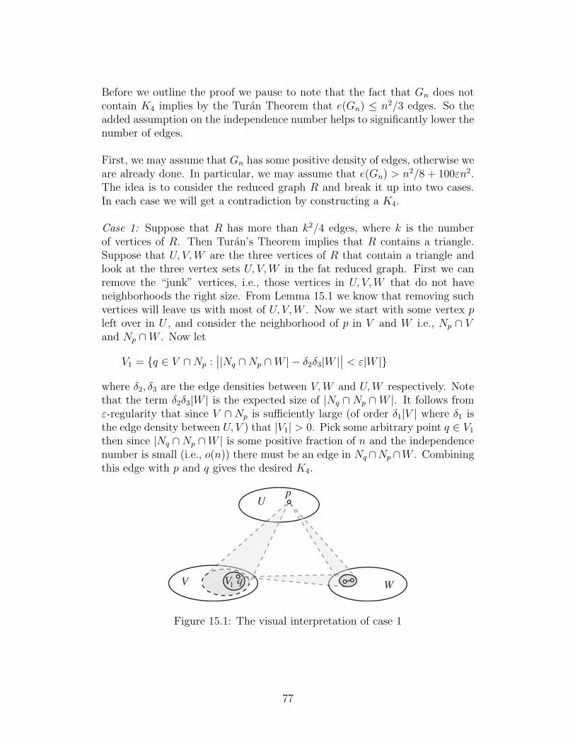
Before we outline the proof we pause to note that the fact that Gn does notcontain K4 implies by the Turan Theorem that e(Gn) ≤ n2/3 edges. So theadded assumption on the independence number helps to significantly lower thenumber of edges.

First, we may assume that Gn has some positive density of edges, otherwise weare already done. In particular, we may assume that e(Gn) > n2/8 + 100εn2.The idea is to consider the reduced graph R and break it up into two cases.In each case we will get a contradiction by constructing a K4.

Case 1: Suppose that R has more than k2/4 edges, where k is the numberof vertices of R. Then Turan’s Theorem implies that R contains a triangle.Suppose that U, V,W are the three vertices of R that contain a triangle andlook at the three vertex sets U, V,W in the fat reduced graph. First we canremove the “junk” vertices, i.e., those vertices in U, V,W that do not haveneighborhoods the right size. From Lemma 15.1 we know that removing suchvertices will leave us with most of U, V,W . Now we start with some vertex pleft over in U , and consider the neighborhood of p in V and W i.e., Np ∩ Vand Np ∩W . Now let

V1 = q ∈ V ∩Np :∣∣|Nq ∩Np ∩W | − δ2δ3|W |

∣∣ < ε|W |

where δ2, δ3 are the edge densities between V, W and U,W respectively. Notethat the term δ2δ3|W | is the expected size of |Nq ∩ Np ∩W |. It follows fromε-regularity that since V ∩ Np is sufficiently large (of order δ1|V | where δ1 isthe edge density between U, V ) that |V1| > 0. Pick some arbitrary point q ∈ V1

then since |Nq ∩Np ∩W | is some positive fraction of n and the independencenumber is small (i.e., o(n)) there must be an edge in Nq ∩Np∩W . Combiningthis edge with p and q gives the desired K4.

U

V W

p

qV1

Figure 15.1: The visual interpretation of case 1

77

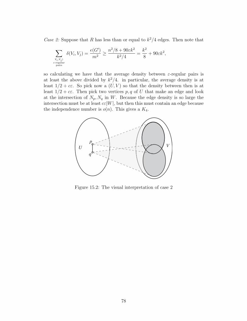
Case 2: Suppose that R has less than or equal to k2/4 edges. Then note that∑Vi,Vj)

ε-regularpairs

δ(Vi, Vj) =e(G′)

m2≥ n2/8 + 90εk2

k2/4=

k2

8+ 90εk2,

so calculating we have that the average density between ε-regular pairs isat least the above divided by k2/4. in particular, the average density is atleast 1/2 + cε. So pick now a (U, V ) so that the density between then is atleast 1/2 + cε. Then pick two vertices p, q of U that make an edge and lookat the intersection of Np, Nq in W . Because the edge density is so large theintersection must be at least cε|W |, but then this must contain an edge becausethe independence number is o(n). This gives a K4.

U Vp

q

Figure 15.2: The visual interpretation of case 2

78

Lecture 16

Ramsey Theory Applications ofthe Regularity LemmaPaul Horn

During the last lecture we examined several applications of the RegularityLemma, including proving the Erdos-Stone theorem, and the Ramsey-Turantheorem. We now turn out attention to applications of the Regularity Lemmain Ramsey theory. Recall that we define the Ramsey number

r(k, k) = min

n :

any 2-coloring of the edges of

Kn contains a monochromatic Kk

.

We are interested in a generalization of this, namely given a graph H we define

r(H) = min

n :

any 2-coloring of the edges of

Kn contains a monochromatic H

.

What types of patterns, H, should have ‘large’ Ramsey numbers, and whatcharacterizations give relatively small Ramsey numbers? Here we examine theinteresting cases which yield linear Ramsey numbers, (i.e. r(H) < c|V (H)|).Some of these results follow relatively easily from the Regularity Lemma. Wenow look at some of these results, and also at some conjectures.

79

16.1 A result on r(H) for graphs with bounded

degree

In 1975 Paul Erdos made the following conjecture: if H is a graph on n verticeswith bounded degree ∆ then r(H) ≤ cn, where c is a constant that dependsonly on ∆. This result was proved in 1983 by Chvatal, Szemeredi, Trotter,and Rodl [17]. We will return to prove this later.

Theorem 16.1. Suppose H has bounded degree δ, |V (H)| = n. Then r(H) ≤cn where c = c(∆)

Note that last time, we showed that if H is a fixed graph (and hence V (H)constant) then H will appear cnh times if H appears in the reduced graphof a large graph G. However now we are talking about H with a constantproportion of the vertices in G and the result is inherently similar concerningthe frequency of appearance of H in G, so long as the degree is bounded. Thistheorem states that r(H) ≤ cn for graphs where the H with bounded degree,however c is a very large constant. The regularity lemma gives this constant

a tower type 22. . .2

with the height of the tower a function of ∆. Subsequentresults have improved this. Nancy Eaton [18], as part of her Ph.D. thesisreduced this to

c(∆) < 22c∆

.

In 2000, R.L. Graham, Rodl, and Rucinski [25] reduced this further still to

c(∆) < 2c∆(log ∆)2 .

These proofs improved the bound by using the idea of the Regularity Lemmawithout applying it directly.

16.2 More results on r(H) for different classes

of graphs

There are many classes of graphs where, while the degree is not bounded, itacts in some sense like the degree is bounded. In some of these cases we canalso get linear Ramsey numbers. Chen and Schelp [9] proved the following

80

Theorem 16.2. If H is a planar graph on n vertices, then r(H) ≤ cn.

A planar graph does not necessarily have bounded degree. For instance, astar graph is planar but does not have bounded degree. The average degree,however, for a planar graph is small. Planar graphs have some other niceproperties as well, for instance a planar graph has to have a vertex with degreeat most 5, and a planar graph can be built by iteratively adding vertices withdegree at most 5. This turns out not to be enough to show the theorem,so a stronger property, called c-arrangeability, is needed. A graph G is c-arrangeable if all vertices of H can be order v1, v2, . . . , vn such that for all i wehave

|j : vi ∼ vj, k > i, vk ∼ j, j < i| ≤ c

It is not immediately obvious that planar graphs satisfy this condition, howeverthis is the condition that is key to showing that planar graphs have a linearRamsey number. c-arrangeability tells us the order to ‘grow’ our graphs usingthe the regularity lemma. Here is a rough sketch of the proof in [9].

At any point, the choices for vi are restricted only by the vj that came beforeit, and will influence the future neighbors of vi. There are only a finite numberof these, and each has a ‘bag’ of possible choices. That is for each vi there isa positive fraction number of vertices in the regular partition that it is beingembedded into that are ‘candidate’ vi, and each of these ‘bags’ restrict thepotential vi. However, since there are only finitely many restrictions, then ε-regularity gives us that there will be a positive-fraction number of candidatesfor vi, so we are in some sense setup to find the next vertex.

Originally when it was shown that planar graphs were c-arrangeable, it was fora very high c, somewhere in the neighborhood of c = 761. However Kiersteadand Trotter [28] showed that planar graphs are 10-arrangeable.

Actually we get a stronger theorem than Theorem 16.2, also due to Chen andSchelp.

Theorem 16.3. If H is c-arrangeable, |V (H)| = n then r(H) ≤ c′n

Rodl and Thomas [35] further extended this to graphs with bounded genus.

Theorem 16.4. If H is of bounded genus, |V (H)| = n, then r(H) ≤ cn.

Despite many nice results that are known concerning graphs with linearlybounded Ramsey numbers, there are still a number of related open conjectures.

81

16.3 Conjectures regarding graphs with lin-

early bounded Ramsey numbers.

Erdos and Burr [7] conjectured the following:

Conjecture 16.1. If H has average degree ∆, with |V (H)| = n, then

r(H) ≤ cn

where c = c(∆).

They also proposed the following, somewhat stronger version.

Conjecture 16.2. Suppose H is a graph, with |V (H)| = n. If, for all sub-graphs H ′ ⊂ H, H ′ has minimum degree less than ∆ then

r(H) ≤ cn

where c = c(∆).

Note that both of these are very closely related to the result of Chvatal, Rodl,Szemeredi, and Trotter given above as Theorem 16.1, which states that if thedegree is bounded by ∆ then the Ramsey numbers are linearly bounded. Inanother direction, Erdos and Burr also made the following conjecture

Conjecture 16.3. If H is the union of t forests, with |V (H)| = n, then

r(H) ≤ cn

where c = c(t).

Recall that a forest is an acyclic graph, or a collection of trees, not necessar-ily connected. A somewhat related conjecture on trees is the following 1963conjecture of Erdos and Sos.

Conjecture 16.4. Every graph on n vertices having at least n(k − 1)/2 + 1edges must contain as a subgraph every tree of k vertices.

82

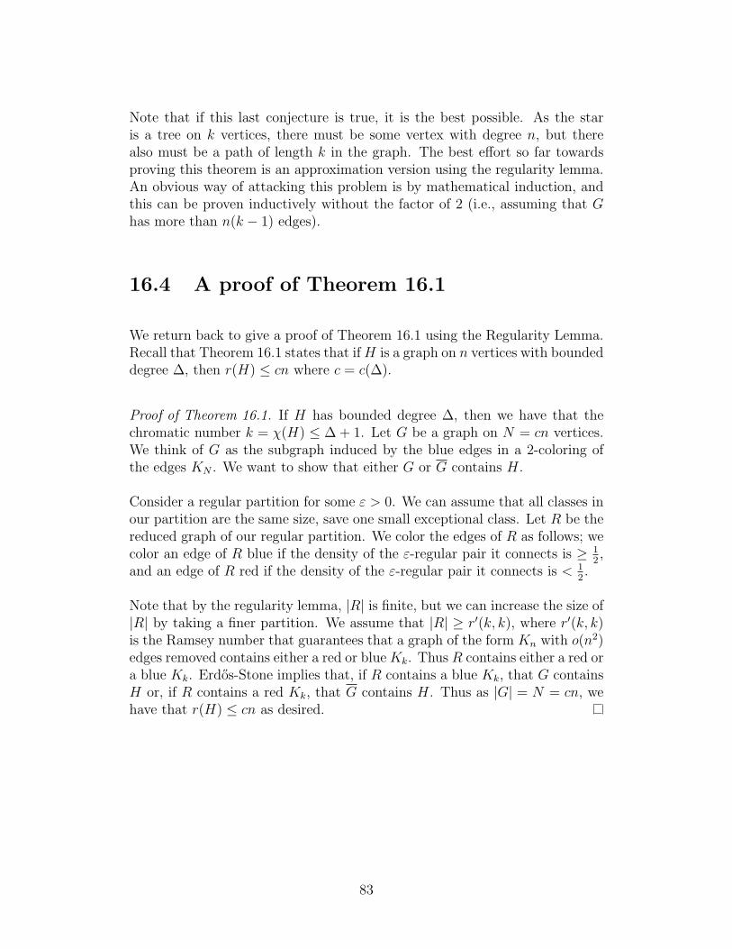
Note that if this last conjecture is true, it is the best possible. As the staris a tree on k vertices, there must be some vertex with degree n, but therealso must be a path of length k in the graph. The best effort so far towardsproving this theorem is an approximation version using the regularity lemma.An obvious way of attacking this problem is by mathematical induction, andthis can be proven inductively without the factor of 2 (i.e., assuming that Ghas more than n(k − 1) edges).

16.4 A proof of Theorem 16.1

We return back to give a proof of Theorem 16.1 using the Regularity Lemma.Recall that Theorem 16.1 states that if H is a graph on n vertices with boundeddegree ∆, then r(H) ≤ cn where c = c(∆).

Proof of Theorem 16.1. If H has bounded degree ∆, then we have that thechromatic number k = χ(H) ≤ ∆ + 1. Let G be a graph on N = cn vertices.We think of G as the subgraph induced by the blue edges in a 2-coloring ofthe edges KN . We want to show that either G or G contains H.

Consider a regular partition for some ε > 0. We can assume that all classes inour partition are the same size, save one small exceptional class. Let R be thereduced graph of our regular partition. We color the edges of R as follows; wecolor an edge of R blue if the density of the ε-regular pair it connects is ≥ 1

2,

and an edge of R red if the density of the ε-regular pair it connects is < 12.

Note that by the regularity lemma, |R| is finite, but we can increase the size of|R| by taking a finer partition. We assume that |R| ≥ r′(k, k), where r′(k, k)is the Ramsey number that guarantees that a graph of the form Kn with o(n2)edges removed contains either a red or blue Kk. Thus R contains either a red ora blue Kk. Erdos-Stone implies that, if R contains a blue Kk, that G containsH or, if R contains a red Kk, that G contains H. Thus as |G| = N = cn, wehave that r(H) ≤ cn as desired.

83

Lecture 17

Extremal Conjectures Relatedto the Regularity Lemma andan Introduction to ExpandersDan Felix

17.1 Open Conjectures in Extremal Graph The-

ory

Before beginning the treatment of expander graphs we will mention some openconjectures in extremal graph theory. In most cases we do have partial results,and the proofs make use of various versions of the Regularity Lemma.

Conjecture 17.1 (Erdos-Sos Conjecture). If a graph G on n vertices hasmore than (k − 1)n/2 edges, then it contains all trees having k edges.

Ajtai, Komlos, and Szemeredi [1] have proven the following approximate ver-sion of this conjecture.

Theorem 17.1. For every ε > 0 there exists an n0 = n0(ε) such that if a graphG on n > n0 vertices has at least (1 + ε)(k − 1)n/2 edges, then it contains alltrees having k edges.

Our next conjecture is also known as Loebl’s Conjecture.

84

Conjecture 17.2 (n/2-n/2-n/2 Conjecture). Let G be a graph on n ver-tices. If G has at least n/2 vertices of degree at least n/2, then G contains alltrees on at most n/2 vertices.

Ajtai, Komlos, and Szemeredi [2] have proven an approximate form of thisconjecture as well.

Theorem 17.2. Let G be a graph on n vertices. For every ε > 0 there existsan n0 = n0(ε) with the following property. If G has at least (1+ ε)n/2 verticesof degree at least (1 + ε)n/2, and if n > n0, then G contains all trees on atmost n/2 vertices.

Yi Zhao may have recently proven this conjecture for all sufficiently largegraphs [45]. A stronger version, conjectured by Komlos and Sos [21], is stillopen.

Conjecture 17.3. Let G be a graph on n vertices. If G has at least n/2vertices of degree at least k, then G contains every tree on at most k vertices.

Lastly, the following strengthening of Dirac’s theorem is still open. Note thatthe kth power of a graph G is the graph obtained from G by adding the edgeu, v if the distance between the vertices u and v is at most k in G. It isso named because the adjacency matrix of the kth power of G is simply thekth power of the adjacency matrix of G, with all nondiagonal nonzero entriesreplaced by 1, and with all diagonal entries replaced by 0.

Conjecture 17.4 (Posa-Seymour Conjecture). Let G be a graph on nvertices with minimum degree at least kn/(k + 1). Then G contains the kthpower of a Hamiltonian cycle.

Komlos, Sarkozy, and Szemeredi have nearly settled this problem [29].

Theorem 17.3. Let G be a graph on n vertices. For every ε > 0 there existsan n0 = n0(ε) with the following property. If G has minimum degree at least(1+ε)kn/(k+1), and if n > n0, then G contains the kth power of a Hamiltoniancycle.

17.2 Network Routing

We now shift our attention to expander graphs and related concepts. Thestudy of these types of graphs, which we will define later, has risen out of

85

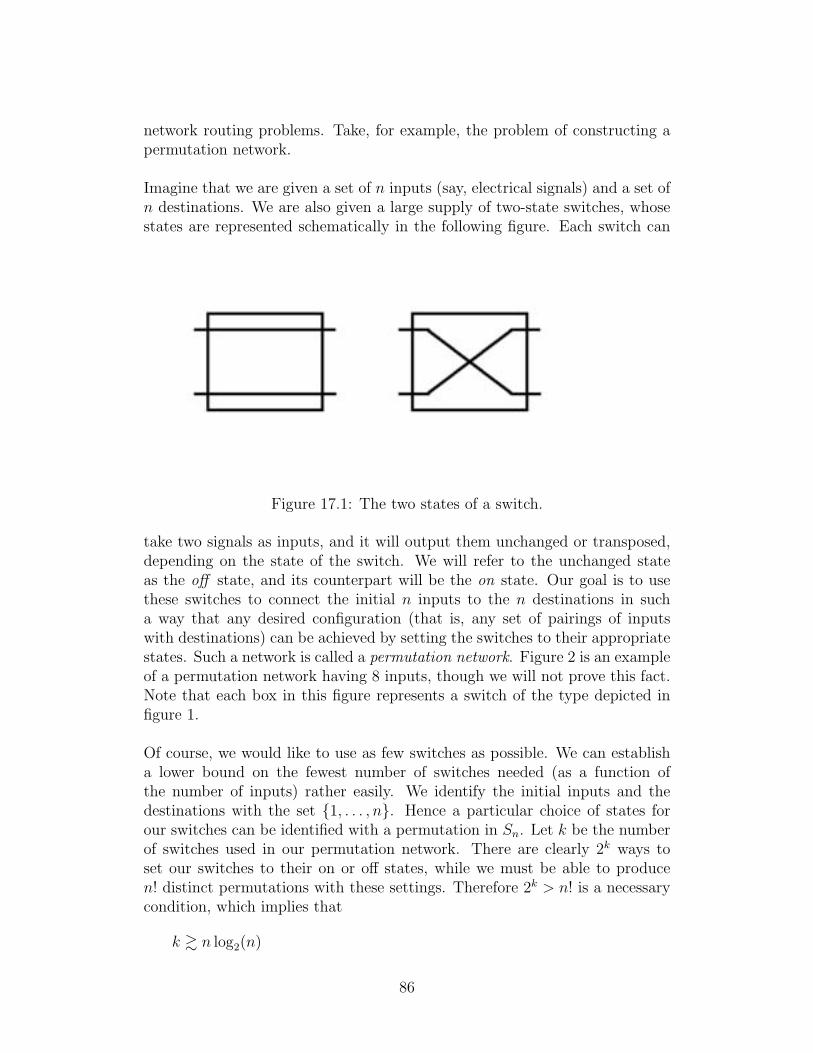
network routing problems. Take, for example, the problem of constructing apermutation network.

Imagine that we are given a set of n inputs (say, electrical signals) and a set ofn destinations. We are also given a large supply of two-state switches, whosestates are represented schematically in the following figure. Each switch can

Figure 17.1: The two states of a switch.

take two signals as inputs, and it will output them unchanged or transposed,depending on the state of the switch. We will refer to the unchanged stateas the off state, and its counterpart will be the on state. Our goal is to usethese switches to connect the initial n inputs to the n destinations in sucha way that any desired configuration (that is, any set of pairings of inputswith destinations) can be achieved by setting the switches to their appropriatestates. Such a network is called a permutation network. Figure 2 is an exampleof a permutation network having 8 inputs, though we will not prove this fact.Note that each box in this figure represents a switch of the type depicted infigure 1.

Of course, we would like to use as few switches as possible. We can establisha lower bound on the fewest number of switches needed (as a function ofthe number of inputs) rather easily. We identify the initial inputs and thedestinations with the set 1, . . . , n. Hence a particular choice of states forour switches can be identified with a permutation in Sn. Let k be the numberof switches used in our permutation network. There are clearly 2k ways toset our switches to their on or off states, while we must be able to producen! distinct permutations with these settings. Therefore 2k > n! is a necessarycondition, which implies that

k & n log2(n)

86

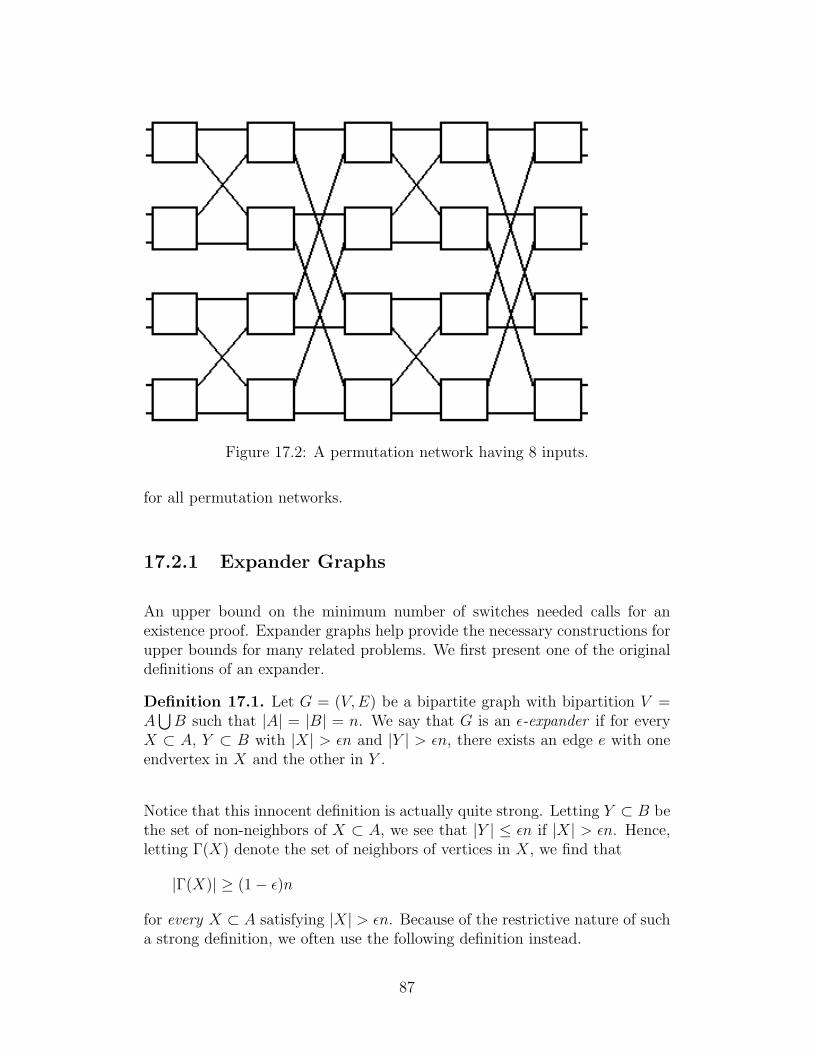
Figure 17.2: A permutation network having 8 inputs.

for all permutation networks.

17.2.1 Expander Graphs

An upper bound on the minimum number of switches needed calls for anexistence proof. Expander graphs help provide the necessary constructions forupper bounds for many related problems. We first present one of the originaldefinitions of an expander.

Definition 17.1. Let G = (V, E) be a bipartite graph with bipartition V =A⋃

B such that |A| = |B| = n. We say that G is an ε-expander if for everyX ⊂ A, Y ⊂ B with |X| > εn and |Y | > εn, there exists an edge e with oneendvertex in X and the other in Y .

Notice that this innocent definition is actually quite strong. Letting Y ⊂ B bethe set of non-neighbors of X ⊂ A, we see that |Y | ≤ εn if |X| > εn. Hence,letting Γ(X) denote the set of neighbors of vertices in X, we find that

|Γ(X)| ≥ (1− ε)n

for every X ⊂ A satisfying |X| > εn. Because of the restrictive nature of sucha strong definition, we often use the following definition instead.

87

Definition 17.2. Let G = (V, E) be a bipartite graph with bipartition V =A⋃

B such that |A| = |B| = n. Let 0 < ε < 1 be any fixed real number. Wesay that G is an ε-expander if

|Γ(X)| > (1 + ε)|X|

for every X ⊂ A satisfying |X| ≤ n/2.

88

Lecture 18

Expander Graphs andSuperconcentratorsSteven Butler

18.1 Expander graphs

In this lecture we will introduce expander graphs and use them to constructsuperconcentrators. Intuitively an expander graph is one in which every subset,which is not too large, has a big neighborhood. More particularly, we say thata graph on n vertices is an expander if there are constants c1, c2 > 0 so that ifS is a subset of the vertices with |S| ≤ c1n then N(S), the neighborhood of Swhich at this time we will define to be vertices adjacent to at least one vertexin S, satisfies |N(S)| ≥ (1 + c2)|S|.

The constant c1 tells us what we mean by a subset which is not too large,in this case we can have up to some positive fraction of the vertices. Theconstant c2 is a measure of how much we are guaranteed to grow by as we lookat neighborhoods. For expander graphs we usually try to make both c1 andc2 large enough to suit our purposes, an example of what this means will begiven below.

We also note that the definition of expander graphs can change depending onhow we define N(S), so for example, we could talk about vertex neighbor-hoods of a set consisting of vertices adjacent to some vertices in a set, or edgeneighborhoods of a set consisting of edges incident to a set.

89

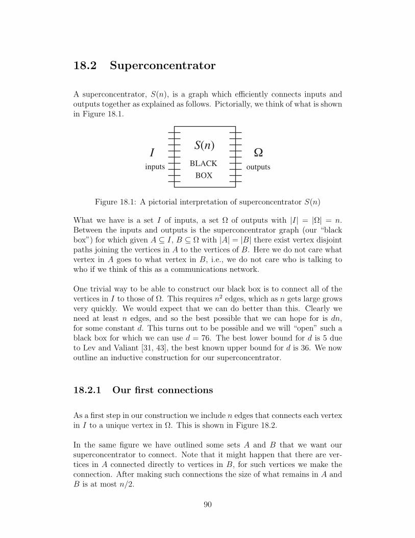
18.2 Superconcentrator

A superconcentrator, S(n), is a graph which efficiently connects inputs andoutputs together as explained as follows. Pictorially, we think of what is shownin Figure 18.1.

I Ωinputs outputsBLACK

BOX

S(n)

Figure 18.1: A pictorial interpretation of superconcentrator S(n)

What we have is a set I of inputs, a set Ω of outputs with |I| = |Ω| = n.Between the inputs and outputs is the superconcentrator graph (our “blackbox”) for which given A ⊆ I, B ⊆ Ω with |A| = |B| there exist vertex disjointpaths joining the vertices in A to the vertices of B. Here we do not care whatvertex in A goes to what vertex in B, i.e., we do not care who is talking towho if we think of this as a communications network.

One trivial way to be able to construct our black box is to connect all of thevertices in I to those of Ω. This requires n2 edges, which as n gets large growsvery quickly. We would expect that we can do better than this. Clearly weneed at least n edges, and so the best possible that we can hope for is dn,for some constant d. This turns out to be possible and we will “open” such ablack box for which we can use d = 76. The best lower bound for d is 5 dueto Lev and Valiant [31, 43], the best known upper bound for d is 36. We nowoutline an inductive construction for our superconcentrator.

18.2.1 Our first connections

As a first step in our construction we include n edges that connects each vertexin I to a unique vertex in Ω. This is shown in Figure 18.2.

In the same figure we have outlined some sets A and B that we want oursuperconcentrator to connect. Note that it might happen that there are ver-tices in A connected directly to vertices in B, for such vertices we make theconnection. After making such connections the size of what remains in A andB is at most n/2.

90

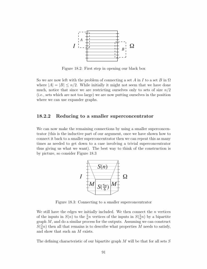
I ΩA

B

Figure 18.2: First step in opening our black box

So we are now left with the problem of connecting a set A in I to a set B in Ωwhere |A| = |B| ≤ n/2. While initially it might not seem that we have donemuch, notice that since we are restricting ourselves only to sets of size n/2(i.e., sets which are not too large) we are now putting ourselves in the positionwhere we can use expander graphs.

18.2.2 Reducing to a smaller superconcentrator

We can now make the remaining connections by using a smaller superconcen-trator (this is the inductive part of our argument, once we have shown how toconnect it back to a smaller superconcentrator then we can repeat this as manytimes as needed to get down to a case involving a trivial superconcentratorthus giving us what we want). The best way to think of the construction isby picture, so consider Figure 18.3

I Ω

S(n)

S( )5n6

M M

Figure 18.3: Connecting to a smaller superconcentrator

We still have the edges we initially included. We then connect the n verticesof the inputs in S(n) to the 5

6n vertices of the inputs in S(5

6n) by a bipartite

graph M , and do a similar process for the outputs. Assuming we can constructS(5

6n) then all that remains is to describe what properties M needs to satisfy,

and show that such an M exists.

The defining characteristic of our bipartite graph M will be that for all sets S

91

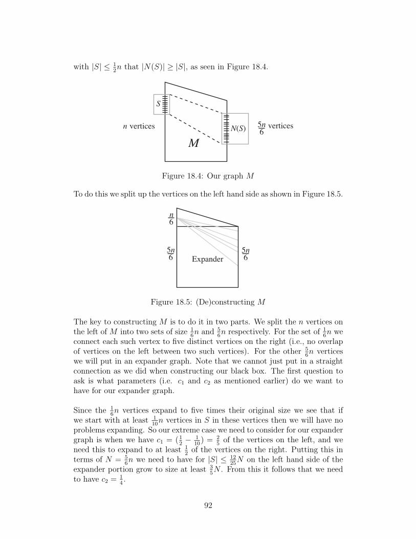
with |S| ≤ 12n that |N(S)| ≥ |S|, as seen in Figure 18.4.

5n6

n

S

N(S)

M

vertices vertices

Figure 18.4: Our graph M

To do this we split up the vertices on the left hand side as shown in Figure 18.5.

5n6

5n6

n6

Expander

Figure 18.5: (De)constructing M

The key to constructing M is to do it in two parts. We split the n vertices onthe left of M into two sets of size 1

6n and 5

6n respectively. For the set of 1

6n we

connect each such vertex to five distinct vertices on the right (i.e., no overlapof vertices on the left between two such vertices). For the other 5

6n vertices

we will put in an expander graph. Note that we cannot just put in a straightconnection as we did when constructing our black box. The first question toask is what parameters (i.e. c1 and c2 as mentioned earlier) do we want tohave for our expander graph.

Since the 16n vertices expand to five times their original size we see that if

we start with at least 110

n vertices in S in these vertices then we will have noproblems expanding. So our extreme case we need to consider for our expandergraph is when we have c1 = (1

2− 1

10) = 2

5of the vertices on the left, and we

need this to expand to at least 12

of the vertices on the right. Putting this interms of N = 5

6n we need to have for |S| ≤ 12

25N on the left hand side of the

expander portion grow to size at least 35N . From this it follows that we need

to have c2 = 14.

92

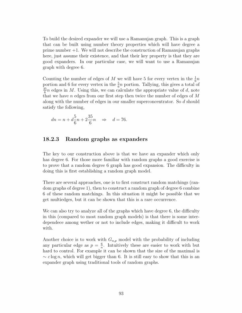
To build the desired expander we will use a Ramanujan graph. This is a graphthat can be built using number theory properties which will have degree aprime number +1. We will not describe the construction of Ramanujan graphshere, just assume their existence, and that their key property is that they aregood expanders. In our particular case, we will want to use a Ramanujangraph with degree 6.

Counting the number of edges of M we will have 5 for every vertex in the 16n

portion and 6 for every vertex in the 56n portion. Tallying, this gives a total of

356n edges in M . Using this, we can calculate the appropriate value of d, note

that we have n edges from our first step then twice the number of edges of Malong with the number of edges in our smaller superconcentrator. So d shouldsatisfy the following,

dn = n + d5

6n + 2

35

6n ⇒ d = 76.

18.2.3 Random graphs as expanders

The key to our construction above is that we have an expander which onlyhas degree 6. For those more familiar with random graphs a good exercise isto prove that a random degree 6 graph has good expansion. The difficulty indoing this is first establishing a random graph model.

There are several approaches, one is to first construct random matchings (ran-dom graphs of degree 1), then to construct a random graph of degree 6 combine6 of these random matchings. In this situation it might be possible that weget multiedges, but it can be shown that this is a rare occurrence.

We can also try to analyze all of the graphs which have degree 6, the difficultyin this (compared to most random graph models) is that there is some inter-dependece among wether or not to include edges, making it difficult to workwith.

Another choice is to work with Gn,p model with the probability of includingany particular edge as p = 6

n. Intuitively these are easier to work with but

hard to control. For example it can be shown that the size of the maximal is∼ c log n, which will get bigger than 6. It is still easy to show that this is anexpander graph using traditional tools of random graphs.

93

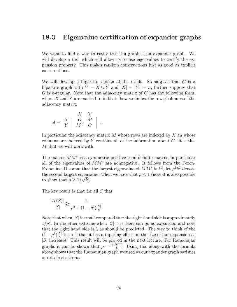
18.3 Eigenvalue certification of expander graphs

We want to find a way to easily test if a graph is an expander graph. Wewill develop a tool which will allow us to use eigenvalues to certify the ex-pansion property. This makes random constructions just as good as explicitconstructions.

We will develop a bipartite version of the result. So suppose that G is abipartite graph with V = X ∪ Y and |X| = |Y | = n, further suppose thatG is k-regular. Note that the adjacency matrix of G has the following form,where X and Y are marked to indicate how we index the rows/columns of theadjacency matrix.

A =

X YX O MY MT O

.

In particular the adjacency matrix M whose rows are indexed by X an whosecolumns are indexed by Y contains all of the information about G. It is thisM that we will work with.

The matrix MM∗ is a symmetric positive semi-definite matrix, in particularall of the eigenvalues of MM∗ are nonnegative. It follows from the Peron-Frobenius Theorem that the largest eigenvalue of MM∗ is k2, let ρ2k2 denotethe second largest eigenvalue. Then we have that ρ ≤ 1 (note it is also possibleto show that ρ ≥ 1/

√k).

The key result is that for all S that

|N(S)||S|

≥ 1

ρ2 + (1− ρ2) |S|n

.

Note that when |S| is small compared to n the right hand side is approximately1/ρ2. In the other extreme when |S| = n there can be no expansion and notethat the right hand side is 1 as should be predicted. The way to think of the(1− ρ2) |S|

nterm is that it has a tapering effect on the size of our expansion as

|S| increases. This result will be proved in the next lecture. For Ramanujan

graphs it can be shown that ρ = 2√

k−1k

. Using this along with the formulaabove shows that the Ramanujan graph we used as our expander graph satisfiesour desired criteria.

94

Lecture 19

Spectral Analysis of ExpanderGraphsKevin Costello

19.1 An Eigenvalue Bound on Expansion for

Bipartite Graphs

Although it is possible to check directly whether a graph is an expander graph,doing so is computationally very expensive since the expansion property mustbe checked for every subset of size at most c1n. Our goal is to prove a theoremwhich will allow us to certify that a bipartite graph is an expander using abound on a single numerical value.

Theorem 19.1. Let G be a k-regular bipartite graph between X and Y with|X| = |Y | = n. Let M be the n×n adjacency matrix of X and Y , and assumethe second largest eigenvalue of MM∗ is at most ρ2k2. Then for all S ⊆ X,

|N(S)||S|

≥ 1

ρ2 + (1− ρ2) |S|n

.

This enables us to feasibly construct expanders using probabilistic algorithms.As mentioned in the previous lecture, a random k-regular bipartite graphis an expander with high probability. Assuming the slightly stronger resultthat random k-regular bipartite graphs will usually also have small ρ, we canconstruct a expander by repeatedly taking random graphs until we find onewith sufficiently small ρ. Alternatively, this theorem can be used to verify that

95

an explicit construction gives an expander graph by bounding the eigenvaluesof that construction.

Proof of Theorem 19.1. Fix S ⊆ X, and let χS

be the indicator function of S,i.e.

χS(x) =

1 if x ∈ S,0 if x /∈ S.

As MM∗ is a symmetric matrix, it has a complete orthonormal set of (left)eigenvectors φi such that φiMM∗ = λ2

i φi. Without loss of generality as-sume the eigenvalues are arranged in decreasing order, so λ0 = k and φ0 =〈 1√

n, 1√

n, . . . , 1√

n〉.

Consider the expression f(S) = 1k2 χS

MM∗χ∗S. On the one hand, we have

1

k2χ

S(MM∗χ∗

S) =

1

k2

( n−1∑i=0

〈χS, φi〉φi

)( n−1∑j=0

〈χS, φj〉λ2

i φ∗j

)=

1

k2

n−1∑i=0

〈χS, φi〉2λ2

i ,

where the latter equality comes from the orthonormality of the φi. But fori > 0 we have that λ2

i ≤ ρ2k2, and we can explicitly compute

〈χS, φ0〉 =

∑x∈S

1√n

=|S|√

n.

Plugging these bounds in, we get that

f(S) =1

k2

(k2|S|2

n+

n−1∑i=1

〈χS, φi〉2λ2

i

)≤ |S|2

n+ ρ2

n−1∑i=1

〈χS, φi〉2.

Since by the Pythagorean Theorem∑〈χ

S, φi〉2 = 〈χ

S, χ

S〉 = |S|, we can

simplify the right hand side down further to get

f(S) ≤ |S|2

n+ ρ2

(|S| − |S|2

n

)= ρ2|S|+ (1− ρ2)

|S|2

n

On the other hand,

f(S) =1

k2

∑u∈S

∑v∈S

|w ∈ T |u ∼ w and v ∼ w|.

96

Equivalently, f(S) is the sum over w ∈ N(S) of the number of pairs of neigh-bors of w in S, so

f(S) =1

k2

∑w∈N(S)

|N(w) ∩ S|2.

Applying the Cauchy-Schwarz inequality with ai = |N(w)∩ S| and bi = 1, weget

f(S) ≥(∑

w∈N(S) |N(w) ∩ S|)2

k2|N(S)|=

(∑

u∈S deg(u))2

k2|N(S)|=

|S|2

|N(S)|2.

Combining the upper and lower bounds on f(S), we have that

|S|2

|N(S)|2≤ ρ2|S|+ (1− ρ2)

|S|2

n.

Dividing by |S| and flipping both sides over, we get

|N(S)||S|

≥ 1

ρ2 + (1− ρ2) |S|n

,

which is the desired result.

19.2 Explicit expanders via Ramanujan Graphs

In the construction of our superconcentrator what we needed to have was alinear expander, one such that the number of edges grows linearly with thenumber of vertices. If we assume that our expander is a regular bipartitegraph, this corresponds to an infinite family of graphs such that n tends toinfinity, but k remains constant.

Theorem 19.1 says that any such family whose second largest eigenvalue issufficiently small will have an expansion property, and the smaller the boundon the eigenvalue the better the expansion property we can prove. Therefore itis desirable to construct families of k-regular graphs whose second eigenvalueis as small as possible. It is a corollary of a result of Alon and Boppara [32]that in any such family

lim infn→∞

λ1 ≥ 2√

k − 1,

97

so the best uniform bound on ρ that we can hope for is ρ = 2√

k−1k

. Individual

graphs satisfying λ1 ≤ 2√

k − 1 are known as Ramanujan Graphs. Familiesof sparse Ramanujan graphs were first constructed using number theoreticmethods [32], but more examples have been constructed, such as the cosetgraph for finite fields [10].

It should be noted that although the Ramanujan Graphs give us the bestpossible eigenvalue bound for expansion, that bound may not itself be optimal,especially for small graphs. For example, our bounds give that a k-regularRamanujan graph will have for any S that

|N(S)||S|

≥ k2

4(k − 1) + (k2−4k+4)|S|n

.

Taking |S| to be small relative to n, this gives a bound of about k|S|/4 for|N(S)|. But for small |S|/n probabilistic methods give that |N(S)| ≈ k|S|(it is unlikely for any one vertex to be adjacent to two members of S). Usingspectral theory alone “cheated” us out of a factor of 4 for small |S|/n.

98

Bibliography

[1] M. Ajtai, J. Komlos, and E. Szemeredi, “On the Erdos-Sos conjecture -an approximate version in the dense case”, manuscript (1991).

[2] M. Ajtai, J. Komlos, and E. Szemeredi, “On a conjecture of Loebl”, Pro-ceedings of the 7th International Conference on Graph Theory, Combina-torics, and Algorithms, (Kalamazoo, Michigan, 1992), 1135-1146, Wiley,New York, 1995.

[3] F.A. Behrend, “On sets of integers which contain no three terms in arith-metical progression.”, Proc. Nat. Acad. Sci. U.S.A. 32 (1946), 331–332.

[4] E.L. Berlekamp, “A construction for partitions which avoid long arith-metic progressions”, Canad. Math. Bull., 11 (1968), 409–414.

[5] Y. Bilu, “Structure of sets with small sumsets”, Structure Theory of SetAddition, Asterisque 258, Soc. Math. France, Montrouge, 1999, 77–108.

[6] J.A. Bondy and M. Simonovits, “Cycles of even length in graphs”, J.Comb. Theory (B) 16 (1974), 97–105.

[7] S.A. Burr and P. Erdos, “On the magnitude of generalized Ramsey num-bers”, Infinite and Finite Sets, Vol. 1, Colloq. Math. Soc., Janos Bolyai,North Holland, Amsterdam/London, 1975.

[8] M. Chang, “A polynomial bound in Freiman’s Theorem”, Duke Mathe-matics Journal, Vol. 113, No.3, 2002, 399–419.

[9] G. Chen, R.H. Schelp, “Graphs with linearly bounded Ramsey numbers”,J. Combin Theory Ser. B 57 (1993) 193–206.

[10] F.R.K. Chung, “Diameters and Eigenvalues”, J. Amer. Math. Soc. 2(1989), 187–196.

[11] F.R.K. Chung, Spectral Graph Theory. CBMS No. 92, American Mathe-matical Society, 1997.

99

[12] F.R.K. Chung and R.L. Graham, “Quasi-random set systems”, J. Amer.Math. Soc. 4 (1991), 151–196

[13] F.R.K. Chung, “Regularity lemmas for hypergraphs and quasi-randomness”, Random Structures Algorithms 2 (1991), no. 2, 241–252.

[14] F.R.K. Chung and R.L. Graham, R “Quasi-random subsets of Zn”, J.Comb. Th. (A) 61 (1992), 64–86.

[15] F.R.K. Chung, R.L. Graham and R.M. Wilson, “Quasi-random graphs”,Combinatorica, 9 (1989), 345–362.

[16] F.R.K. Chung and L. Lu, “An upper bound for the Turan numbert3(n, 4)”, J. Comb. Theory(A) 87 (1999), 381–389.

[17] C. Chvatal, E. Szemeredi, W.T. Trotter, Jr. and V. Rodl, “The Ramseynumber of a graph with bounded maximum degree”, J. Combin TheorySer. B 34 (1983), no. 3, 239–243.

[18] N. Eaton, “Ramsey number for sparse graphs”, Discrete Math, 185, 63–75(1998).

[19] P. Erdos, “Extremal problems in graph theory”, Theory of Graphs andits Applications, Proc. Symp. (Smolenice, 1963) (M. Fielder, ed.), 29–36.New York: Academic Press, 1965.

[20] P. Erdos, “On sequences of integers no one of which divides the productof two others and on some related problems”, Mitt. Forsch.-Inst. Math.Mech. Univ. Tomsk 2 (1938), 74–82.

[21] P. Erdos, Z. Furedi, M. Loebl, and V.T. Sos, “Discrepancy of trees”,Studia Sci. Math. Hungar. 30 (1995) no. 1-2, 47-57.

[22] P. Erdos and A.H. Stone, “On the structure of linear graphs”, Bull. Amer.Math. Soc. 52 (1946), 1087–1091.

[23] W.T. Gowers, “A new proof of Szemeredi’s theorem”, Geom. Funct. Anal.,11 (2001), no. 3, 465–588.

[24] W.T. Gowers, “Some Unsolved Problems in Additive/CombinatorialNumber Theory”, www.dpmms.cam.ac.uk/˜wtg10/addnoth.survey.dvi.

[25] R. Graham, V. Rodl and A. Rucinski, “On graphs with linear Ramseynumbers”, J. Graph Theory 35 (2000), no. 3, 176–192.

[26] B. Green and T. Tao, “The primes contain arbitrarily long arithmeticprogressions”, front.math.ucdavis.edu/math.NT/0404188.

100

[27] R. Horn and C. Johnson, “Matrix Analysis”, Cambridge University Press,1985.

[28] H.A. Kierstead and W.T. Trotter, “Planar graph coloring with an unco-operative partner”, J. Graph Theory 18 (1994) 569–584.

[29] J. Komlos, G.N. Sarkozy, and E. Szemeredi, “On the Posa-Seymour con-jecture”, Journal of Graph Theory 29 (1998), 167-176.

[30] J. Komlos and M. Simonovits, Szemeredi’s Regularity Lemma and itsapplications in graph theory, Combinatorics, Paul Erdos is eighty, Vol.2 (Keszthely, 1993), 295–352, Bolyai Soc. Math. Stud., 2, Janos BolyaiMath. Soc., Budapest, 1996.

[31] G. Lev, “Size bounds for parallel algorithms for networks”, Ph.D. Thesis,Department of Computer Science, University of Edinburg.

[32] A. Lubotzky, R. Philips, and P. Sarnak, “Ramanujan Graphs”, Combi-natorica, 9 (1988), 261–277.

[33] M.B. Nathanson, Additive Number Theory: Inverse Problems and the Ge-ometry of Sumsets Graduate Texts in Mathematics 165, Springer-Verlag,1996.

[34] V. Rodl, P. Frankl, “The uniformity lemma for hypergraphs”, GraphsCombin. 8 (1992) 309–312.

[35] V. Rodl and R. Thomas, “Arrangeability and clique subdivisions”,The mathematics of Paul Erdos, II, 236–239, Algorithms Combin., 14,Springer Berlin, 1997.

[36] K.F. Roth, “On certain sets of integers.”, J. London Math. Soc. 28 (1953),104–109.

[37] I.Z. Ruzsa and E. Szemeredi. “Triple systems with no six points carry-ing three triangles.” Colloqui Mathematica Societatis Janos Bolyai, 18.Combinatorics, Keszthely (Hungary), 1976, 199–245.

[38] S. Shelah, “Primitive recursive bounds for van der Waerden numbers”, J.Amer. Math. Soc. 1 (1988), no. 3, 683–697.

[39] J. Solymosi. “Note on a Generalization of Roth’s Theorem”. Discrete andComputational Geometry: the Goodman-Pollack Festschrift. Ed. Aranovet. al. Springer, Berlin, 2003.

[40] E. Szemeredi, “On sets of integers containing no four elements in arith-metic progression”, Acta Math. Acad. Sci. Hungar. 20 (1969), 89-104

101

[41] E. Szemeredi, “On sets of integers containing no k elements in arithmeticprogression”, Acta Arith. 27 (1975), 299-345.

[42] P. Turan, “Eine Extremalaufgabe aus der Graphentheorie”, Mat. Fiz.Lapok 48 (1941), 436–452.

[43] L.G. Valiant, “A scheme for fast parallel communication”, SIAM J. Com-put. 11 (1982), 350–361.

[44] B.L. van der Waerden, “Beweis einer Baudetschen Vermutung”, NieuwArch. Wisk. 15 (1927) 212–216.

[45] Y. Zhao, “Proof of the (n/2-n/2-n/2) conjecture for large n”,www2.math.uic.edu/˜zhao/publications/lobel conj.pdf.

102

Index

arithmetic progressions, 5, 84-term, 63–683-term, 25generalized arithmetic progres-

sions, 36

c-arrangeable, 81Cartesian product, 53Cauchy-Schwarz, 12–13cyclic graph, 40

deviation, 51–54, 57dev l, 55

discrepancy, 55, 57bound by deviation, 58

edge density, 7, 9hypergraphs, 30

eigenvalue certification, 94, 95ε-regular, 9

(3, 1), 30, 32(3, 2), 31, 32

Erdos, Paul, 8Erdos-Stone Theorem, 72expander graphs, 87, 89

fat reduced graph, 73Freiman isomorphism, 36Freiman Theorem, 36

graphs, 6

Hungarian method, 20hypergraphs, 27, 29

index, 15, 33induced matchings, 19, 20intersection graphs, 47, 48

inverse problem, 36irregular edges, 10

kth power of G, 85

Loebl’s Conjecture, 84log∗ n, 19

µk(H), µk(H), 50

n/2-n/2-n/2 conjecture, 85network routing, 85

Ok, 48, 51

Paley graphs, 46–47, 49permutation network, 86positive upper density, 5

quasi-random, 7, 14, 41–43, 45hypergraphs, 43

Ramanujan graph, 93Ramsey graphs, 47Ramsey number, 79random graphs

expanders, 93reduced graph, 73Regularity Lemma, 6, 11, 15

hypergraph version, 33limitations of, 7proof, 15–19

sameness graph, 52(6, 3), 22sumset, 35superconcentrator, 90Szemeredi partition, 10

103

Turan’s Theorem, 69, 72

van der Waerden, 7

104