1

Working Paper Departamento de Economía Economic Series 13 – 06 Universidad Carlos III of Madrid August 2013 Calle Madrid, 126

28903 Getafe, Madrid

“THE COMPARISON OF NORMALIZATION PROCEDURES BASED ON DIFFERENT

CLASSIFICATION SYSTEMS”

Yunrong Li, and Javier Ruiz-Castillo•  Departamento de Economía, Universidad Carlos III

Abstract

In this paper, we develop a novel methodology within the IDCP measuring framework for comparing normalization procedures based on different classification systems of articles into scientific disciplines. Firstly, we discuss the properties of two rankings, based on a graphical and a numerical approach, for the comparison of any pair of normalization procedures using a single classification system for evaluation purposes. Secondly, when the normalization procedures are based on two different classification systems, we introduce two new rankings following the graphical and the numerical approaches. Each ranking is based on a double test that assesses the two normalization procedures in terms of the two classification systems on which they depend. Thirdly, we also compare the two normalization procedures using a third, independent classification system for evaluation purposes. In the empirical part of the paper we use: (i) a classification system consisting of 219 sub-fields identified with the Web of Science subject-categories; an aggregate classification system consisting of 19 broad fields, as well as a systematic and a random assignment of articles to sub-fields with the aim of maximizing or minimizing differences across sub-fields; (ii) four normalization procedures that use the field or sub-field mean citations of the above four classification systems as normalization factors, and (iii) a large dataset, indexed by Thomson Reuters, in which 4.4 million articles published in 1998-2003 with a five-year citation window are assigned to sub-fields using a fractional approach. The substantive results concerning the comparison of the four normalization procedures indicate that the methodology can be useful in practice.

Acknowledgements. This is the second version of a Working Paper with the same title that appeared in this series in February 2013. The authors acknowledge financial support by Santander Universities Global Division of Banco Santander. Ruiz-Castillo also acknowledges financial help from the Spanish MEC through grant ECO2010-19596. Conversations with Ludo Waltman are greatly appreciated. However, all remaining shortcomings are the authors’ sole responsibility.

                                                                                                                         

2

I. INTRODUCTION

Differences in publication and citation practices have been known for decades to create serious

difficulties for the comparison of raw citation counts across different scientific disciplines. Since the

early eighties various normalization proposals have been suggested (see the review by Schubert and

Braun, 1996). Moreover, the normalization problem has recently attracted renewed interest.1

Consequently, there is a need to develop methods for the comparison of the performance achieved by

different normalization procedures in empirical situations.

Lacking information on the citing side, we focus on normalization procedures of the target or

cited-side variety, where each procedure is based on a priori given classification system of publications

in the periodical literature into a set of scientific disciplines. The paper studies the evaluation of

alternative normalization procedures in two scenarios. In the first one, there is only a single

classification system for the implementation as well as the evaluation of two (or more) normalization

procedures. In this case, all that is needed is a method for assessing the performance of the contesting

normalization procedures using the single classification system for evaluation purposes. In the second

scenario, there are two (or more) classification systems for the implementation and the evaluation of

two (or more) normalization procedures. As far as we know, this is the first paper that presents a

complete discussion of this case (see, however, the contributions by Sirtes, 2012, and Waltman and Van

Eck, 2013, that will be discussed below).

Given a classification system, we evaluate the performance of normalization procedures using the

measurement framework recently introduced in Crespo et al. (2013a), where the number of citations

received by an article is a function of two variables: the article’s underlying scientific influence, and the

                                                                                                                         1 Among the target, or cited-side variety of normalization procedures, see Glanzel (2011), Radicchi et al. (2008), Radicchi and Castellano (2012), and Crespo et al. (2013a, b), as well as the review of the percentile rank approach by Bornmann and Max (2013). Among the source, or citing-side variety, see inter alia Zitt and Small (2008), Moed (2010), Leydesdorff and Opthof (2010), and Waltman and Van Eck (2012a).

3

discipline to which it belongs. Consequently, the citation inequality of the distribution consisting of all

articles in all disciplines –the all-sciences case– is the result of two forces: differences in scientific influence

within each homogeneous discipline, and differences in citation practices across the set of

heterogeneous disciplines. Essentially, as we will see below, the effect of the latter on citation inequality

is captured by an IDCP term –where IDCP stands for citation Inequality attributable to Differences in

Citation Practices.

A key aspect of this framework is that it serves to evaluate any set of normalization procedures in

terms of any given classification system as required in the first scenario. The evaluation can take a

graphical, or a numerical form.2 In this paper, we establish that the graphical approach does not provide

a complete ranking, i.e. we show that there are situations in which a pair of normalization procedures is

non-comparable according to the graphical criterion. We also establish that the rankings according to

the two approaches are logically independent, that is, we show that there exists at least one pair of

normalization procedures that are ordered differently by the two rankings.

The canonical example of the second scenario arises in the presence of a number of classification

systems at different aggregate levels. Assume for simplicity that there are only two hierarchically nested

classification systems into what we call sub-fields and fields, so that every sub-field at the lower

aggregation level belongs to only one field at the higher aggregate level. The question we study in this

paper is how to compare one normalization procedure based at the sub-field level with another based

at the field level. The problem is that we only know how to assess alternative normalization procedures

using a single classification system for evaluation purposes. Therefore, the performance of the first

                                                                                                                         2 Both forms have been previously used in two instances: (i) to compare the performance of different normalization procedures based on the same classification system (Crespo et al., 2013a, b, and Li et al., 2013), and (ii) to compare two types of normalization procedures, namely, those target procedures in which the disciplines’ mean citations in different classification systems are used as normalization factors, and a variety of source normalization procedures independent of any classification system (Waltman and Van Eck, 2013).

4

procedure evaluated at the sub-field level cannot be directly compared with the performance of the

second procedure evaluated at the field level. Our solution to this problem is the introduction of a new

ranking based on a double test that assesses both normalization procedures in terms of the two

classification systems on which they depend. For a procedure to dominate the other according to the

double test, it should perform better than the other under both classification systems.

This idea is applicable to the comparison of any two normalization procedures based on different

classification systems independently of the method followed for their evaluation. However, it should be

remembered that in our measuring framework the evaluation of normalization procedures could take a

graphical and a numerical approach. Therefore, in our case we must introduce two new rankings, each

of them relying on a double test that compares the two normalization procedures using for evaluation

purposes the two classification systems on which they depend. For a procedure to strongly dominate

another according to the graphical (or the numerical) approach it should exhibit a better graphical (or

numerical) performance under both classification systems. We establish that the two rankings are

logically independent; therefore, strict dominance according to one ranking does not necessarily imply

dominance according to the second.

This strategy deserves two closely related comments. Firstly, satisfying either of the two

dominance criteria is a strong requirement. Consequently, we expect that neither of the two new

rankings is complete. Secondly, Sirtes (2012) first suggested that the assessment of two classification-

system-based normalization procedures would be generally biased in favor of the normalization

procedure based on the system used for evaluation purposes. Waltman and van Eck (2013) concur with

this idea, and provide further arguments about the possibility of this bias. In a double test, the presence

of a bias of this type would favor the first (and the second) procedure under comparison when the first

(and the second) classification system is used for evaluation purposes. Therefore, the bias would

5

increase the probability that the two procedures are non-comparable. In any case, we confirm that

neither of the two rankings is complete.

In order to avoid the bias, Waltman and van Eck (2013) compare source and target normalization

procedures using an independent classification system for evaluation purposes. On our part, we believe

that this is a recommendation worth pursuing. Thus, in the second scenario we suggest the comparison

of any pair of classification-system-based normalization procedures using two strategies: the double

tests that only involve the two classification systems on which the normalization procedures are based,

and the evaluation in terms of a third classification system. Therefore, to illustrate this methodology in

empirical situations we need to specify a number of elements, namely: (i) a minimum of three

classification systems; (ii) a minimum of two classification-system-based normalization procedures, and

(iii) a rich enough dataset.

(i) We use two types of classification systems. Firstly, we use two nested classification systems at

the field and the sub-field aggregation levels. Secondly, following Zitt et al. (2005) we focus on a pair of

classification systems that organize the available data in two polar ways: assigning papers to sub-fields

in a systematic manner, so as to make the differences between sub-fields as large as possible; or

assigning papers to sub-fields in a random manner, so as to make the differences between sub-fields as

small as possible. We refer to them as the systematic and random assignments at the sub-field level.

(ii) As far as normalization procedures are concerned, recall that, since the inception of

Scientometrics as a field of study, differences in citation practices across scientific disciplines in the all-

sciences case are usually taken into account by choosing the world mean citation rates in each discipline

as normalization factors (see inter alia Moed et al., 1985, 1988, 1995, Braun et al., 1985, Schubert et al.,

1983, 1987, 1988, Schubert and Braun, 1986, 1996, and Vinkler 1986, 2003). More recently, other

contributions support this traditional procedure on different grounds (Radicchi et al., 2008, Radicchi

6

and Castellano, 2012a, b, Crespo et al., 2013a, b, and Li et al., 2013). Consequently, in this paper we

choose this type of normalization procedure for every one of the four classification systems introduced

in the previous paragraph.3

(iii) Using a dataset of approximately 4.4 million articles published in all scientific disciplines in

1998-2003 with a five-year citation window, we identify the sub-fields at the lowest aggregation level

permitted by our data with the 219 Web of Science subject categories distinguished by Thomson

Reuters. As is well known, a practical problem is that documents in Thomson Reuters databases are

assigned to sub-fields via the journal in which they have been published. Many journals are assigned to

a single sub-field, but many others are assigned to two, three, or more sub-fields. There are two

alternatives to deal with this problem: a fractional strategy, according to which each publication is

fractioned into as many equal pieces as necessary, with each piece assigned to a corresponding sub-

field; and a multiplicative strategy in which each paper is wholly counted as many times as necessary in

the several sub-fields to which it is assigned. Fortunately, Crespo et al. (2013b) establishes that the effect

on citation inequality of differences in citation practices at the sub-field level according to the two

strategies is very similar, so that it suffices to work with one of the two alternatives. In this paper we

focus on the fractional strategy.

A second well known difficulty is that there is no generally agreed-upon Map of Science that

allows us to climb from the sub-field up to other aggregate levels (see inter alia Small, 1999, Boyack et

al., 2005, Leydesdorff, 2004, 2006, Leydersdorff and Rafols, 2009, and Waltman et al., 2012b as well as

the references they contain). Among the many alternatives, in this paper we consider an intermediate

level consisting of 19 broad fields taken from Albarrán et al. (2011), a contribution that borrows from

the schemes recommended by Tijssen and van Leeuwen (2003) and Glänzel and Schubert (2003) with

                                                                                                                         3 As indicated in the concluding section, the methods developed in this paper can be equally used for the comparison of other types of normalization procedures.

7

the aim of maximizing the possibility that a power law represents the upper tail of the citation

distributions involved. It is not claimed that this scheme provides an accurate representation of the

structure of science. It is rather a convenient simplification for the discussion of aggregation issues in

this paper.

The remaining part of this paper is organized into five Sections. Section II summarizes the

measurement framework introduced in Crespo et al. (2013a), and presents the estimates of the effect on

citation inequality of differences in citation practices across the fields and sub-fields included in our

four classification systems. Section III is devoted to the comparison of normalization procedures using

a single classification system for evaluation purposes within the graphical and the numerical approach.

Section IV introduces the two double tests for the comparison of any pair of normalization procedures

using two classification systems for evaluation purposes. Section V discusses the empirical results on

the comparison of our four normalization procedures using both the two double tests, as well as the

strategy recommended by Waltman and van Eck (2013). Finally, Section VI offers some concluding

remarks.

II. THE EFFECT ON CITATION INEQUALITY OF DIFFERENCES IN CITATION PRACTICES ACROSS SCIENTIFIC DISCIPLINES

II.1. A Measurement Framework

Every classification system K consists of D disciplines, indexed by d = 1…, D. Let C be the initial

citation distribution consisting of the citations received by M articles. For simplicity, we assume that

every article in C is assigned to a single discipline. Let Md be the number of articles in discipline d, so

that Σd Md = M. Denote each discipline citation distribution by c d = {cdi} with i = 1,…, Md, where cdi is

the number of citations received by article i in discipline d. The original citation distribution is simply

the union of all the discipline distributions, that is, C = ∪d c d.

8

Of course, the problem is that every discipline is characterized by idiosyncratic publication and

citation practices. Consequently, the direct comparison of raw citation counts between articles

belonging to different disciplines is plagued with difficulties. In this paper, we measure the effect of

differences in citation practices using a simple model introduced in Crespo et al. (2013a). As we will

presently see, given a classification system K, in the implementation of this model using an additively

decomposable inequality index the citation inequality attributed to differences in citation practices

across disciplines is captured by a between-group inequality term –denoted IDCP(K)– in a certain

partition by discipline and citation quantile.

Partition each citation distribution c d into Π quantiles, cπd, of size Md/Π, indexed by π = 1,…, Π.

Thus, c d = (c1d,…, cπd,…, cΠd). Let µπd be the average citation of quantile cπd, and let µπ

d be the

vector where each article in quantile cπd is assigned the average citation µπd. For every π, consider the

distribution mπ = (µπ1,…, µπ

d,…, µπD) of size M/Π. Under the assumptions of the model in Crespo

et al. (2013a), for each π the citation inequality of mπ ,

I(mπ) = I(µπ1,…, µπ

d,…, µπD), (1)

is attributed to differences in citation practices across disciplines at that quantile. Therefore, any

weighted average of the expressions I(mπ) over all quantiles constitutes a good measure of the

phenomenon we are interested in.

For reasons explained in Crespo et al. (2013a), it is convenient to work with a certain member of

the so-called Generalized Entropy family of citation inequality indices, the index I1. This index has the

9

important property that, for any partition of the population into sub-groups, the overall citation

inequality is additively decomposable into a within- and a between-group term, where the within-group

term is a weighted sum of the sub-group citation inequality terms with weights that add up to one.

Using this index, it can be shown that the citation inequality of the initial distribution, I1(C), can be

expressed as the sum of three terms, one of which is the IDCP term.4 For classification system K, this

term is defined as follows:

IDCP(K) = Σπ vπ I1(mπ) = Σπ vπ I1(µ

π1,…, µπ

d,…, µπD), (2)

where vπ = Σd vπ

d , and vπd is the share in the total citations of discipline d of the citations received by

articles in quantile cπd. Thus, vπ is the share of total citations in the all-sciences case received by articles

in quantile cπd for all disciplines, and Σπ vπ = 1. Therefore, Eq 2 indicates that IDCP(K) is a weighted

average of the key expressions in (1), with weights vπ that add up to one. 5 It should be noted that, due

to the skewness of science, in practical applications the weights vπ tend to increase dramatically with π.

II. 2. Classification Systems

As indicated in the Introduction, we work with four classification systems.

1. System A consists of 219 sub-fields, indexed by s = 1,…, 219, identified with the

corresponding Web of Science categories distinguished by Thomson Reuters. Let Ns be the number of                                                                                                                          4 As far as the two remaining terms in the decomposition are concerned, one refers to the citation inequality that takes place

within the c πd quantiles, while the other measures the citation inequality in the distribution where each article in any discipline is assigned the mean citation of the quantile to which it belongs. For high Π, the first term is expected to be small, while the second –capturing the skewness of science in the all-sciences case– is expected to be large. For details, see Crespo et al. (2013a). 5 Naturally, both the weighting system vπ and the distributions m π depend on the classification system we use for evaluation

purposes. However, for simplicity we do not express this dependency by writing vπ(K) and m π(K) in each case. Unless otherwise indicated, writing IDCP(K) is enough for our purposes.

10

articles in sub-field s in system A, so that Σs Ns = M, and let us denote sub-field s citation distribution

by c s = {csi} with i = 1,…, Ns.

2. Consider the following systematic assignment of publications into the 219 sub-fields of system

A. Start by ordering all articles in the dataset from the least to the most cited, assigning the most highly

cited articles to the smallest sub-field in A. We proceed in this fashion until the largest sub-field is

assigned the least cited articles.6 The classification system based on this systematic assignment is

denoted by S. Sub-field s citation distribution in system S is denoted by cSs = {cSsi} with i = 1,…, Ns,

and s = 1,…, 219.

3. The third classification system corresponds to the random assignment of publications into the

219 sub-fields of system A. We start by randomly selecting one sub-field in A, whose size is denoted by

N1. Then, we randomly draw N1 articles from the dataset, leaving the rest for the next step. We proceed

in this way, using each time the articles remaining after the previous random draws, until the last sub-

field is assigned the articles left at the next-to-last step. The classification system based on this random

assignment is denoted by R. Sub-field s citation distribution in system R is denoted by cRs = {cRsi} with i

= 1,…, Ns, and s = 1,…, 219.

4. System B consists of 19 fields, indexed by f = 1,…, 19, obtained by aggregation of the 219 sub-

fields in system A according to the rule suggested in Albarrán et al. (2011). Let us denote by Nf = Σs∈f

Ns the number of articles in field f in system B. For any f, the field citation distribution c f is the union of

sub-fields in that field, that is, c f = ∪s∈f c s = {cfg} with g = 1,…, Nf.

                                                                                                                         6 When we proceed in the opposite direction, that is, beginning with the assignment of the most highly cited articles to the largest sub-field, we end up with a very large number of sub-fields consisting entirely of uncited articles.

11

Note that the systematic and random assignments provide a test to verify whether the IDCP

method works well in practice. Under the systematic (random) classification system differences

between sub-fields would be at a maximum (minimum). Therefore, we expect IDCP(S) to be well

above IDCP(A) and IDCP(B), while IDCP(R) is expected to be well below IDCP(A) and IDCP(B).

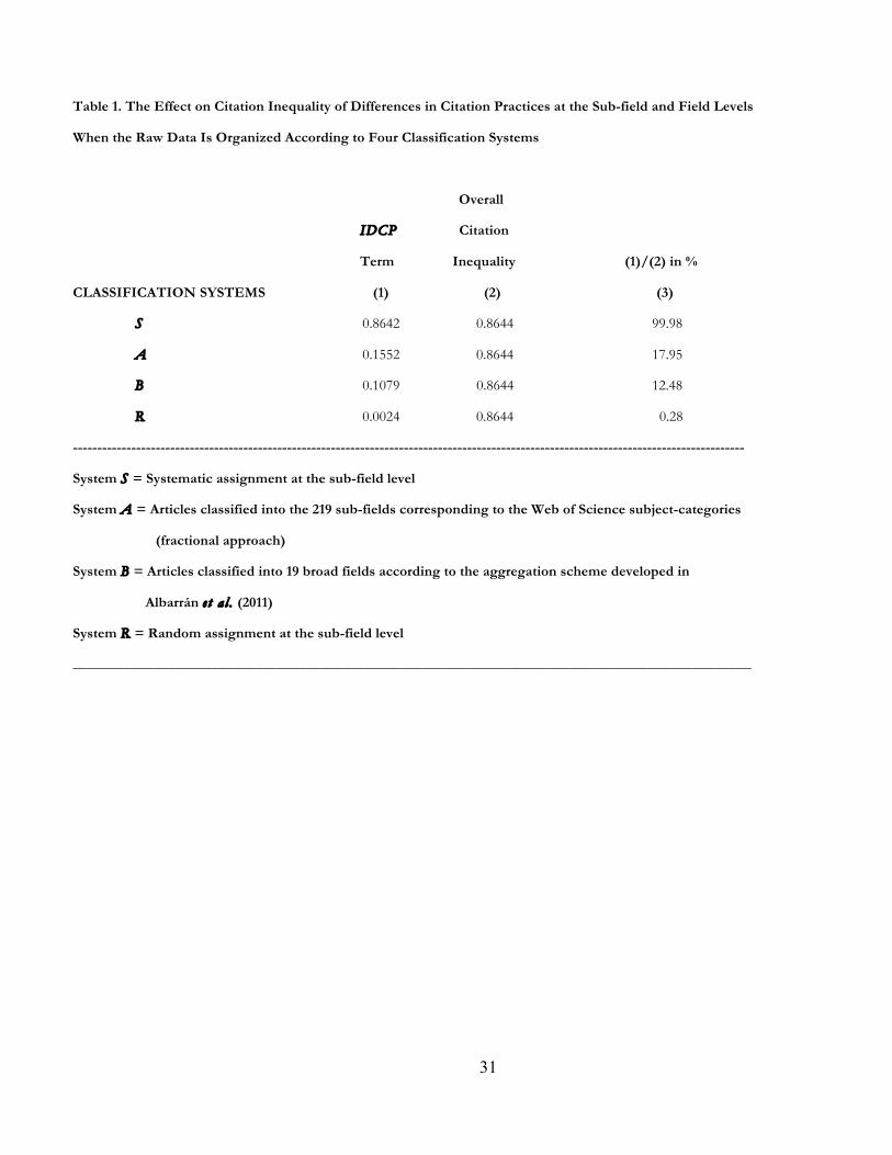
Table 1 includes the values for the IDCP term for the four classification systems when the number of

quantiles Π is equal to 1000 –a choice maintained in the sequel.

Table 1 around here

Three comments are in order. Firstly, since the 4.4 million articles in the dataset are simply

differently organized in the four cases and our citation inequality index is invariant to data

permutations, overall citation inequality is the same for all classification systems. This is the value

0.8644 that appears in column 2 in Table 1. Secondly, it should be noted that the results in row A are

taken from Crespo et al. (2013b). They indicate that the IDCP(A) term represents, approximately, 18%

of overall citation inequality. As expected, the IDCP term represents a smaller proportion of overall

citation inequality when articles are classified into broad fields: IDCP(B)/I1(C) = 12.5%. Thirdly, it can

be concluded that the IDCP method responds very well to the two polar cases in the sense that

IDCP(S) represents practically 100% of overall citation inequality, while IDCP(R) is barely above zero

(see column 3 in Table 1).

III. THE EVALUATION OF NORMALIZATION PROCEDURES IN TERMS OF A GIVEN CLASSIFICATION SYSTEM

III.1. Normalization Procedures

Let us denote by µA

s, µSs, and µR

s the average citation of sub-field s in systems A, S, and R,

respectively. The procedures that use such means as normalization factors at the sub-field level are

12

denoted by NA, NS, and NR, respectively. The normalization of every article i in sub-field s within its

respective system proceeds as follows:

cA*si = csi/µAs in system A;

cS*si = cSsi/µS

s in system S;

cR*si = cRsi/µR

s in system R.

Similarly, denote by µBf the mean citation of field f in system B. Of course, for any f we have µB

f = Σs∈f

(Ns/Nf) µA

s. The normalization of every article g in field f proceeds as follows:

cB*fg = cfg/µBf in system B.

Of course, for any f we have c*f = {c*fg} = ∪s∈f c*s = ∪s∈f {c*si}. After normalization by procedure NK,

for K = S, A, B, and R, the IDCP terms and the citation distributions in the all-sciences case are

denoted by IDCPNK(K) and CK*.

We are also interested in evaluating every procedure using other classification systems that are

different from the one on which it is based. Let us start by evaluating procedure NA in terms of system

S. Note that, for every article i in sub-field s in system S, there exists some article j in some sub-field r in

system A such that cSsi = crj. Therefore, for the evaluation of NA in terms of S the normalization of

each article i in sub-field s in system S proceeds as follows:

cAS*si = crj/µA

r.

In this case, the IDCP term after normalization is denoted by IDCPNA(S). Next, to evaluate NA in

terms of system B, note that, for every article g in field f in system B, there exists some article k in some

sub-field t in system A such that cBfg = ctk. Therefore, for the evaluation of NA in terms of B the

normalization of each article g in sub-field f in system B proceeds as follows:

13

cAB*fg = ctk/µA

t.

In this case, the IDCP term after normalization is denoted by IDCPNA(B). We leave to the reader how

to evaluate any other procedure in terms of a system that is different from the one on which the

procedure is based.

In general, given any normalization procedure NK and a classification system G –not necessarily

equal to K– the IDCP after normalization is written IDCPNK(G). Similarly, the citation distribution in

the all-sciences case after normalization by NK evaluated in terms of system G ≠ K is denoted by CKG*.

Note that, given any procedure NK, CKG* for G ≠ K is a mere permutation of distribution CK*. Hence,

given NK, total citation inequality of the normalized citation distribution in the all-sciences case is

independent of the system used for evaluation purposes, i.e. for any K, I1(CKG*) = I1(C

K*) for all G ≠ K.

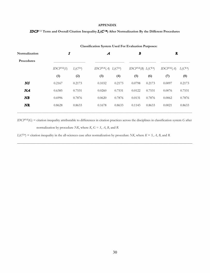
For later reference, the values for IDCPNK(G) and I1(CK*) are presented in the Appendix.

To facilitate the description of the graphical and numerical evaluation approaches, it is essential

to realize that, for any K and G, the term IDCPNK(G) is a weighted average of expressions capturing the

citation inequality of the normalized citation distributions according to procedure NK attributable to

differences in citation practices across disciplines in system G. Formally, we have:

IDCPNK(G) = Σπ v*π(G) I1NK[m*π(G)], (3)

where the asterisk in v*π(G) and m*π(G) denotes that we are referring to a normalized distribution

within classification system G, while the superscript in I1NK[.] indicates that the normalization takes

place according to NK. Using this notation, we can proceed to discuss the graphical and numerical

evaluation approaches.

14

III. 2. The Graphical Method

It should be remembered that, given the skewness of science, for any normalization procedure

and any classification system, the weights v*π(.) in Eq. 3 tend to increase dramatically with π. Therefore,

it is convenient to make the evaluation before the weighting system is applied, namely, in terms of the

expressions I1NK[m*π(G)] that, for any π, capture the effect of differences in citation practices in system

G after normalization by procedure NK. Thus, given any pair of procedures NK and NL and a single

classification system G –not necessarily distinct from K or L– for evaluation purposes, we proceed by

comparing I1NK[m*π(G)] and I1

NL[m*π(G)] at any π.

We say that NK is uniformly better than NL under system G if I1NK[m*π(G)] < I1

NL[m*π(G)] for all π,

that is, if the curve I1NK[.] as a function of π is uniformly below the curve I1

NL[.]. In this case, we write

{NK >I(G) NL}, while in the opposite case we write {NL >I(G) NK}. However, the avoidance of the

weighting issue comes at a cost: when the two curves exhibit one (or more) intersections, then we must

conclude that two procedures are non-comparable according to this criterion, in which case we write

{NK Non>I(G) NL}.

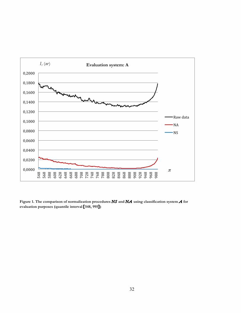
Consider Example 1 where K = S, L = A, and G = A, illustrated in Figure 1 (Since expressions

I1NS[.] and I1

NA[.] are very high for many quantiles in the lower tail of citation distributions and in the

last quantiles in the upper tail, for clarity Figure 1 only includes quantiles π in the interval [548, 995]).

Three points should be noted. Firstly, the citation inequality due to differences in citation practices at

any π in the raw data organized according to system A is measured by the curve I1[mπ(A)] in black in

Figure 1. Secondly, normalization gives rise to a clear decrease of the curves I1NK[m*π(A)] for both NK

15

= NS, NA below I1[mπ(A)]. Thirdly, in Figure 1 the curve I1

NS[m*π(A)] is always below

I1NA[m*π(A)], indicating that {NS >I(A) NA} according to the graphical approach.7

Next, consider Example 2 where K = A, L = B, and G = B, illustrated in Figure 2 (for the

interval π∈[574, 1000]).8 This is an interesting case, where we expect the procedure constructed at the

lowest aggregate level, NA, to perform better than NB. However, this needs to be confirmed in

practice. As a matter of fact, Figure 2 illustrates that, relative to the situation with the raw data, both

procedures perform well but, because they repeatedly intersect, they are non-comparable. Thus, we

conclude that {NA Non>I(B) NB}, which shows that, in general, the ranking >I(.) is not complete.

Figures 1 and 2 around here

III. 3. The Numerical Method

An alternative way to compare any pair of procedures NK and NL under any given classification

system G, is by comparing the corresponding IDCP terms after normalization, that is, by comparing

IDCPNK(G) and IDCPNL(G). We find more useful expressing the result as the percentage that the

differences [IDCPNK(G) - IDCP(G)] and [IDCPNL(G) - IDCP(G)] represent relative to the initial

situation, IDCP(G). Thus, given any pair of procedures NK and NL and a single system G for

evaluation purposes, we say that NK is numerically better than NL under system G if the following condition

is satisfied:

[IDCP(G) - IDCPNK(G)]/IDCP(G) > [IDCP(G) - IDCPNL(G)]/IDCP(G). (4)

                                                                                                                         7 Of course, one could apply formal dominance methods to compare the two curves. However, we do not find it essential in the sequel, where a simple graphical approach will be applied. It should be noted that, in all cases whenever one normalization procedure dominates another one in the subset of quantiles shown in a Figure, the dominance takes place uniformly over the entire domain. 8 Note that the units in which magnitudes are measured along the vertical axis in every Figure are quite different. This precludes the direct, visual comparability between them.

16

In this case, we write {NK >II(G) NL}, while if inequality (4) goes in the opposite direction, then we

write {NL >II(G) NK}. Note that the ranking of normalization procedures in the numerical approach

is always complete, that is, for any pair of normalization procedures to be evaluated in terms of any

classification system, we can always say whether one procedure is numerically better than the other.

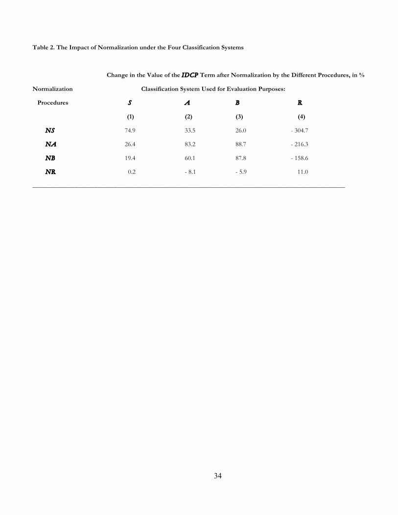
To see how numerical comparisons work in practice we need to know the consequences of

applying the different normalization procedures under all classification systems. Using the values of

IDCPNK(G) in the Appendix, Table 2 presents the change in the IDCP term before and after each of

the normalization operations. Consider, for example, the case in which normalization procedure NA is

applied to the data organized according to system S. The consequences are captured by IDCPNA(S) in

row NA and column 1 in the Appendix. In turn, recall that IDCP(S) = 0.8642 (see column 1 in row S

in Table 1). Taking into account criterion (4), we are interested in the percentage change in the IDCP

term before and after applying NA in S, that is, in the expression

100 [IDCP(S) - IDCPNA(S)]/IDCP(S) = 100 (0.8642 – 0.6385)/0.8642 = 26.1.

The value of this expression appears in row NA and column 1 in Table 2, indicating that the effect of

differences in citation practices across sub-fields in system S has been reduced by 26.1% as a

consequence of normalization by NA. This compares, for example, with the reduction of 19.4% caused

by normalization with NB using again system S for evaluation purposes (see row NB and column 1 in

Table 2). On the other hand, the figures in columns 2, 3, and 4 in row NA are the values in expression

100 [IDCP(K) - IDCPNA(K)]/IDCP(K),

when the evaluation system is K = A, B, and R rather than S.

Table 2 around here

17

Once the meaning of each entry in Table 2 has been clarified, we are ready to compare

normalization procedures in some paradigmatic examples using the numerical approach. Consider again

Example 1 where K = S, L = A, and G = A. Since IDCPNS(A) = 0.1032 and IDCPNA(A) = 0.0260 (see

column 3 in the Appendix), NA exhibits a better numerical performance than NS under system A, that

is, {NA >II(A) NS} (see column 2 in Table 2). This shows that the rankings >I and >II are

independent because we have simultaneously {NS >I(A) NA} and {NA >II(A) NS}.

On the other hand, consider again Example 2 where procedures NA and NB are compared in

terms of system B. It is observed in Table 2 that NA performs numerically better than NB, so that

{NA >II(B) NB}. This shows that the two approaches are complementary and can be profitably used

together: although the two procedures are non-comparable according to the graphical approach, NA is

seen to perform numerically better than NB when system B is used for evaluation purposes in both

cases.

IV. THE EVALUATION OF NORMALIZATION PROCEDURES USING DIFFERENT CLASSIFICATION SYSTEMS

IV. 1. The First Double Test

Consider the comparison of any two procedures NK and NL. The problem, of course, is that

they cannot be compared in terms of their own classification system. In other words, the terms

IDCPNK(K) and IDCPNL(L) are not directly comparable because the classification systems K and L are

different. Economists will note that this problem is akin to the lack of comparability of a country’s

Gross National Product (GNP) in two different time periods in nominal terms, say GNP1 and GNP2.

The reason is that GNP1 is the value of production in period 1 at prices of that period, while GNP2 is

18

the value of production in period 2 at prices of that period.9 For a meaningful comparison, GNP in the

two periods must be expressed at common prices; that is, comparisons must be made only in real terms.

However, we face what is known as an index number problem: which prices should be used in the

comparison? For best results, production in both periods should be expressed at prices of period 1 and

at prices of period 2. If GNP2 at prices of period 1 is greater than GNP1, and GNP2 is greater than

GNP1 at prices of period 2, then we say that GNP in real terms has unambiguously increased at both

periods’ prices. If both inequalities go in the opposite direction, then we say that GNP in real terms has

unambiguously decreased. Otherwise, namely, if one inequality favors one period and the other

inequality favors the other, then we say that GNP in both periods is non-comparable in real terms.

In our context, any pair of procedures, NK and NL, should be evaluated using both systems K

and L. In the graphical approach, the extension gives rise to five possibilities.

(i) We say that NK strongly dominates NL in the graphical sense if the first procedure performs

uniformly better than the second using both systems for evaluation purposes, namely, if {NK >I(K)

NL} and {NK >I(L) NL}. In this case, we write {NK DI(K , L) NL}.

(ii) If the opposite of (i) is the case, then we write {NL DI(K, L) NK}.

(iii) If NK performs uniformly better than NL according to one of the systems, but the two

procedures are uniformly non-comparable according to the second system, namely if, for example,

{NK >I(K) NL} and {NK Non>I(L) NL}, then we say that NK weakly dominates NL in the graphical

sense and write {NK WDI(K , L) NL}.

(iv) If the opposite of (iii) is the case, then we write {NL WDI(K , L) NK}.

                                                                                                                         9 Of course, the same situation arises when we compare the GNP of two different countries in nominal terms. In this case production in the two countries is evaluated at their respective price systems.

19

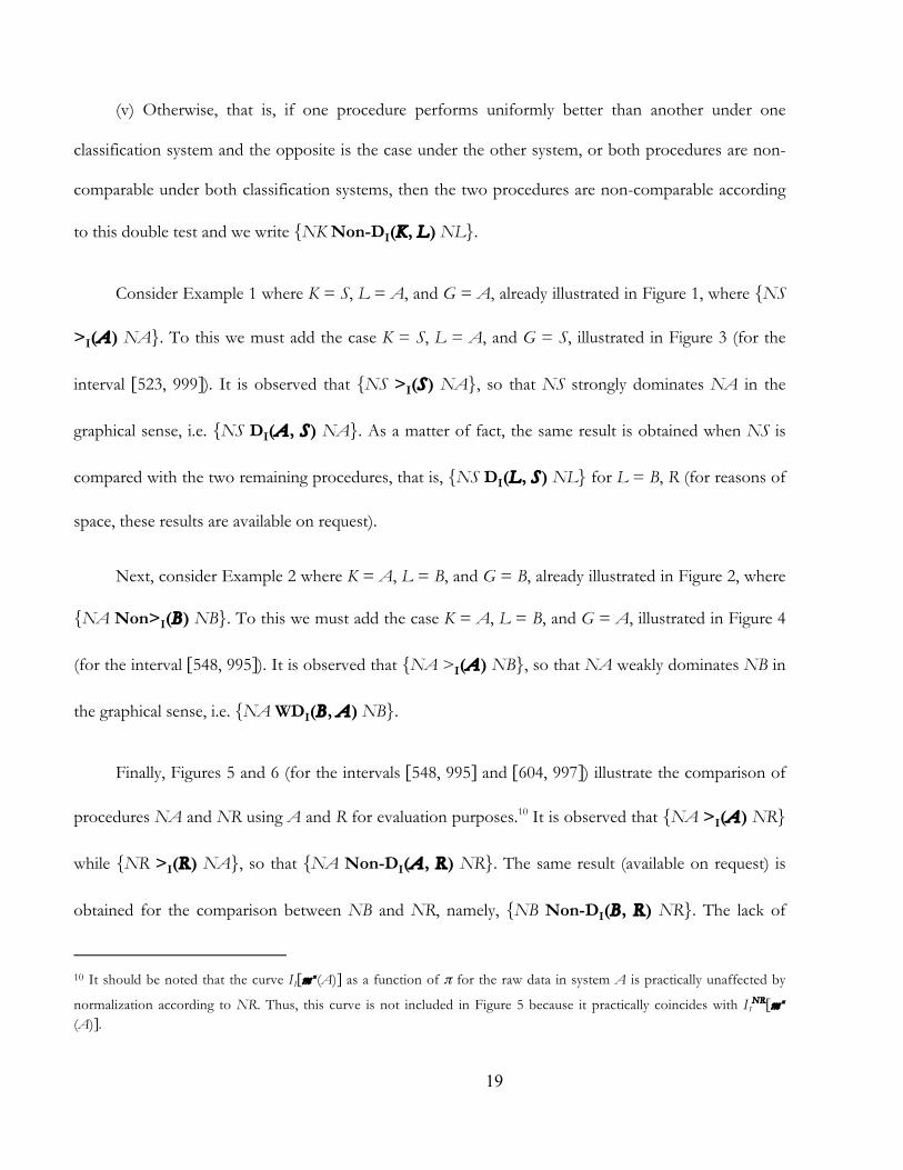
(v) Otherwise, that is, if one procedure performs uniformly better than another under one

classification system and the opposite is the case under the other system, or both procedures are non-

comparable under both classification systems, then the two procedures are non-comparable according

to this double test and we write {NK Non-DI(K , L) NL}.

Consider Example 1 where K = S, L = A, and G = A, already illustrated in Figure 1, where {NS

>I(A) NA}. To this we must add the case K = S, L = A, and G = S, illustrated in Figure 3 (for the

interval [523, 999]). It is observed that {NS >I(S) NA}, so that NS strongly dominates NA in the

graphical sense, i.e. {NS DI(A , S) NA}. As a matter of fact, the same result is obtained when NS is

compared with the two remaining procedures, that is, {NS DI(L , S) NL} for L = B, R (for reasons of

space, these results are available on request).

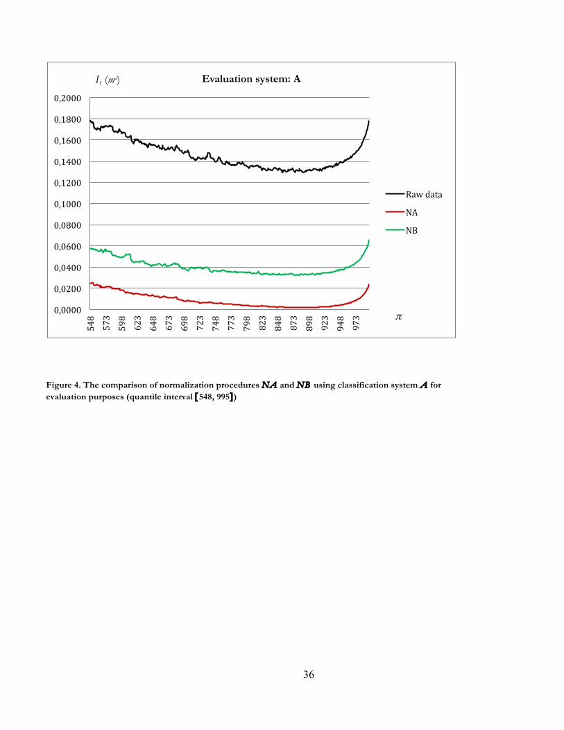
Next, consider Example 2 where K = A, L = B, and G = B, already illustrated in Figure 2, where

{NA Non>I(B) NB}. To this we must add the case K = A, L = B, and G = A, illustrated in Figure 4

(for the interval [548, 995]). It is observed that {NA >I(A) NB}, so that NA weakly dominates NB in

the graphical sense, i.e. {NA WDI(B , A) NB}.

Finally, Figures 5 and 6 (for the intervals [548, 995] and [604, 997]) illustrate the comparison of

procedures NA and NR using A and R for evaluation purposes.10 It is observed that {NA >I(A) NR}

while {NR >I(R) NA}, so that {NA Non-DI(A , R) NR}. The same result (available on request) is

obtained for the comparison between NB and NR, namely, {NB Non-DI(B , R) NR}. The lack of

                                                                                                                         10 It should be noted that the curve I1[m π(A)] as a function of π for the raw data in system A is practically unaffected by

normalization according to NR. Thus, this curve is not included in Figure 5 because it practically coincides with I1NR[m π

(A)].

20

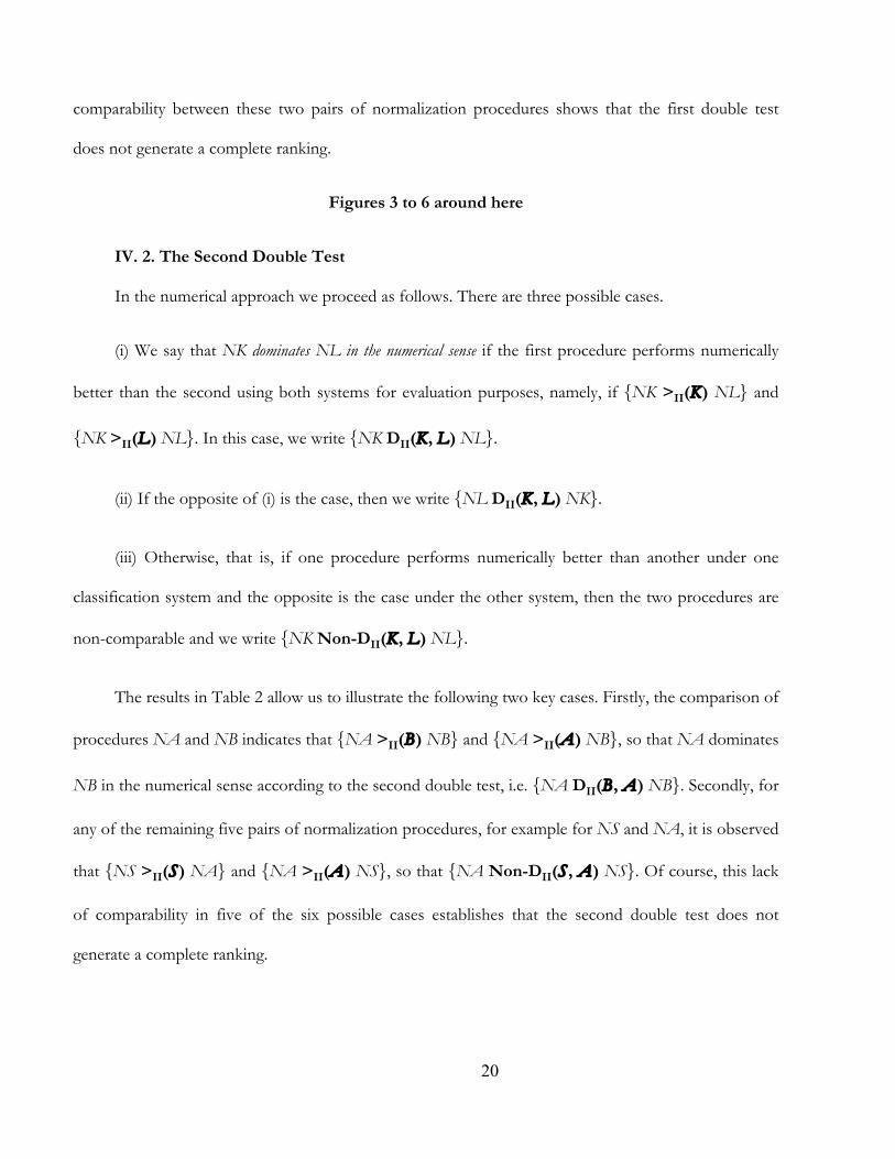
comparability between these two pairs of normalization procedures shows that the first double test

does not generate a complete ranking.

Figures 3 to 6 around here

IV. 2. The Second Double Test In the numerical approach we proceed as follows. There are three possible cases.

(i) We say that NK dominates NL in the numerical sense if the first procedure performs numerically

better than the second using both systems for evaluation purposes, namely, if {NK >II(K) NL} and

{NK >II(L) NL}. In this case, we write {NK DII(K , L) NL}.

(ii) If the opposite of (i) is the case, then we write {NL DII(K , L) NK}.

(iii) Otherwise, that is, if one procedure performs numerically better than another under one

classification system and the opposite is the case under the other system, then the two procedures are

non-comparable and we write {NK Non-DII(K , L) NL}.

The results in Table 2 allow us to illustrate the following two key cases. Firstly, the comparison of

procedures NA and NB indicates that {NA >II(B) NB} and {NA >II(A) NB}, so that NA dominates

NB in the numerical sense according to the second double test, i.e. {NA DII(B , A) NB}. Secondly, for

any of the remaining five pairs of normalization procedures, for example for NS and NA, it is observed

that {NS >II(S) NA} and {NA >II(A) NS}, so that {NA Non-DII(S , A) NS}. Of course, this lack

of comparability in five of the six possible cases establishes that the second double test does not

generate a complete ranking.

21

Finally, recall that {NS DI(A , S) NA} while {NA Non-DII(A , S) NS}. This shows that the

two double tests are independent: strong dominance of NS over NA in the graphical sense does not

imply dominance in the same direction in the numerical sense. Similarly, in spite of the fact that {NA

DII(B , A) NB} we have that {NA WDI(B , A) NB}, that is, dominance in the numerical sense is

compatible with just weak dominance in the graphical sense.

V. DISCUSSION

In this Section, we compare the six pairs of normalization procedures making precise in each

case how far we can go with the two double tests, and which are the additional insights arising from the

use of a third classification system for evaluation purposes as recommended by Waltman and van Eck

(2013).

1. As we saw in Table 1, practically all citation inequality under system S is attributable to

differences in citation practices. The other side of this coin is that, when highly cited sub-fields within S

are normalized by high mean citations, differences in citation practices at every π are drastically

reduced. As a matter of fact, the curve I1NS[m*π(K)] as a function of π is always below I1

NL[m*π(K)] for

all NL ≠ NS, and all K = S, A, B, and R (see, for example, Figures 1 and 3 for NL = NA and K = A,

S). In other words, procedure NS achieves the best possible results according to the first double test

under the graphical approach: {NS DI(S , L) NL} for all L ≠ S. On the other hand, NS performs also

numerically better than the other procedures under system S itself. However, once the weighting

system is taken into account and the evaluation is made in terms of any system L ≠ S, we observe that

the terms IDCPNS(L) are very high (see column 1 in the Appendix). In particular, this implies that NS is

non-comparable with NA and NB according to the second double test, i.e. {NL Non-DII(S , L) NS}

for L = A, B.

22

Thus, taking together the results of the two double tests, it would appear that the polar procedure

NS exhibits a somewhat better performance than the two regular procedures NA and NB. In this

rather worrisome situation, the evaluation of NS versus NA and NB in terms of an independent

classification system becomes very relevant indeed. For the comparison with NA, for example, it is

observed that {NA >II(R) NS}. Exactly the same result is obtained for the comparison with NB (see

column 4 in Table 2). Therefore, the weakness of NS relative to the regular procedures only manifests

itself when the numerical evaluation uses an independent classification system.11

2. When articles are randomly assigned to sub-fields in system R, almost none of the citation

inequality is attributable to differences in citation practices across sub-fields because the vast majority

of citation inequality takes place within sub-fields. At the same time, since sub-field mean citations in R

are very similar to each other, normalization by NR has practically no consequences when articles are

organized according to the other systems. The implication is that the curve I1[mπ(K)] as a function of π

for the raw data organized according to any system K ≠ R is practically unaffected by normalization

according to NR (see, for example, Figure 5 for the case K = A). Similarly, in the numerical approach

normalization according to NR introduces almost no correction or even increases the IDCPNR(K) term

when K ≠ R (see the last row in Table 2). Thus, in particular, {NK >I(K) NR} and {NK >II(K) NR}

when K = A, B. However, the minimal impact of NR works in its favor when the evaluation is done

using system R itself. Thus, {NR >I(R) NK} for K = A, B in the graphical approach (see Figure 6 for

the case K = A). Similarly, {NR >II(R) NK} for all K = A, B in the numerical approach (see column 4

in Table 2). This leads to the conclusion that NR is non-comparable with NA and NB according to

both double tests –a rather undesirable situation.                                                                                                                          11 Note that {NA >II(B) NS} and {NB >II(A) NS} (see columns 3 and 2 in Table 2). However, it could be argued that systems A and B are not entirely independent.

23

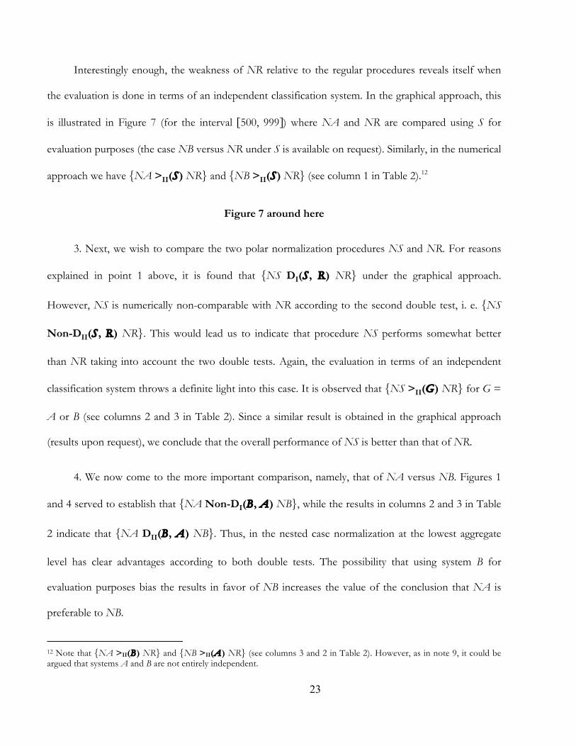
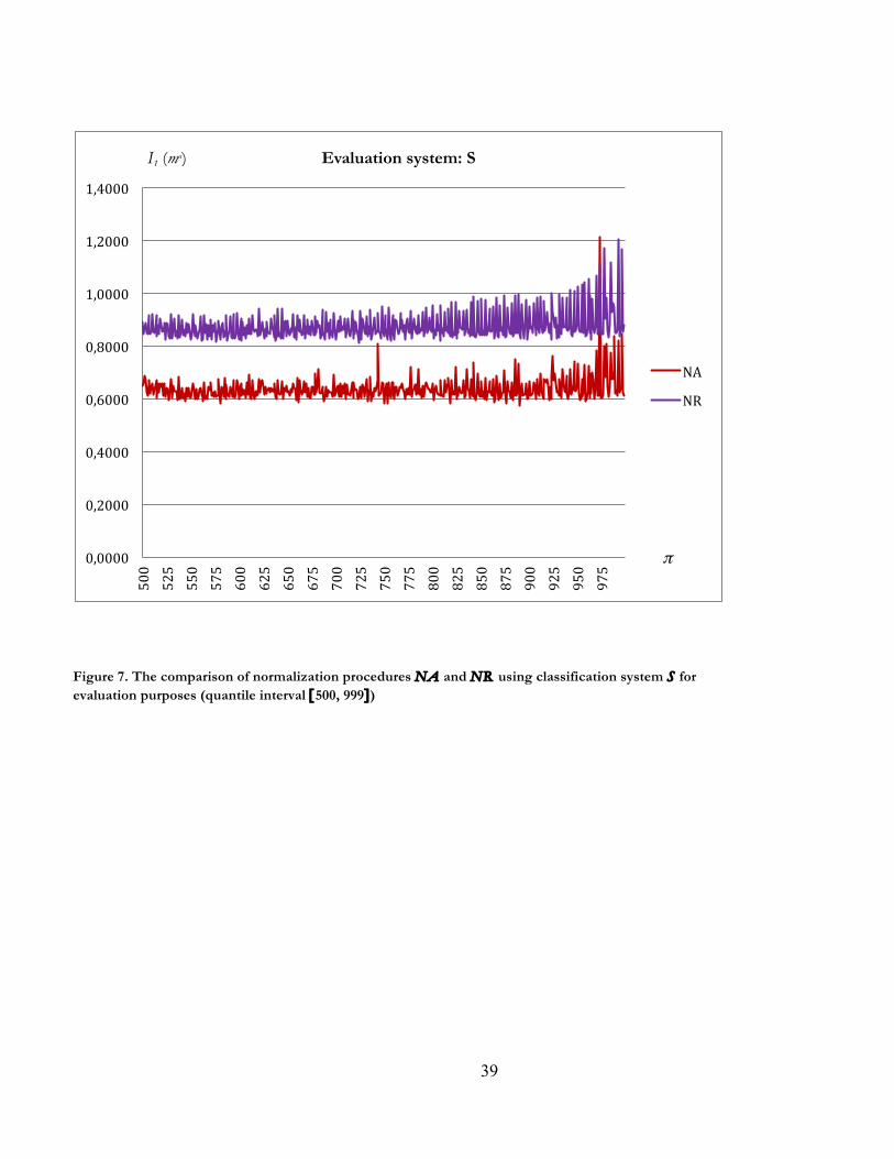
Interestingly enough, the weakness of NR relative to the regular procedures reveals itself when

the evaluation is done in terms of an independent classification system. In the graphical approach, this

is illustrated in Figure 7 (for the interval [500, 999]) where NA and NR are compared using S for

evaluation purposes (the case NB versus NR under S is available on request). Similarly, in the numerical

approach we have {NA >II(S) NR} and {NB >II(S) NR} (see column 1 in Table 2).12

Figure 7 around here

3. Next, we wish to compare the two polar normalization procedures NS and NR. For reasons

explained in point 1 above, it is found that {NS DI(S , R) NR} under the graphical approach.

However, NS is numerically non-comparable with NR according to the second double test, i. e. {NS

Non-DII(S , R) NR}. This would lead us to indicate that procedure NS performs somewhat better

than NR taking into account the two double tests. Again, the evaluation in terms of an independent

classification system throws a definite light into this case. It is observed that {NS >II(G) NR} for G =

A or B (see columns 2 and 3 in Table 2). Since a similar result is obtained in the graphical approach

(results upon request), we conclude that the overall performance of NS is better than that of NR.

4. We now come to the more important comparison, namely, that of NA versus NB. Figures 1

and 4 served to establish that {NA Non-DI(B , A) NB}, while the results in columns 2 and 3 in Table

2 indicate that {NA DII(B , A) NB}. Thus, in the nested case normalization at the lowest aggregate

level has clear advantages according to both double tests. The possibility that using system B for

evaluation purposes bias the results in favor of NB increases the value of the conclusion that NA is

preferable to NB.

                                                                                                                         12 Note that {NA >II(B) NR} and {NB >II(A) NR} (see columns 3 and 2 in Table 2). However, as in note 9, it could be argued that systems A and B are not entirely independent.

24

However, two further points should be noted. Firstly, NB performs numerically well not only

under system B itself, but also when we evaluate it using system A: 60% of the effect on citation

inequality of differences in citation practices at the sub-field level is eliminated via NB (see column 2 in

Table 2). This is important because the availability of data often restricts us to a high aggregate level.

The lesson is clear: whenever the only option is to normalize at a relatively high aggregate level, we

should do it knowing that the reduction of the problem –even at the sub-field level– is non-negligible.

Secondly, NA also performs better than NB in terms of S, i.e. {NA >II(S) NB} (see column 1 in Table

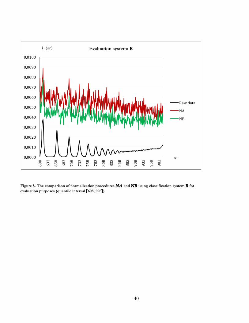
2), and {NA >I(S) NB} (results available on request). However, as illustrated in column 4 in Table 2

and in Figure 8 (quantile interval [608, 996]), the opposite is the case when the evaluation is done in

terms of R, i.e. {NB >II(R) NA}, and {NB >I(R) NA}. This serves as a warning that evaluations of

normalization procedures using an independent classification system may lead us towards a conclusion

that contradicts the results obtained under the two double tests and other independent evaluations.

Figure 8 around here

V. CONCLUSIONS

In this paper, we have extended the methodology for the evaluation of classification-based-

normalization procedures. For this purpose, we have used the measurement framework introduced in

Crespo et al. (2013a) where the effect of differences in citation practices across scientific disciplines is

well captured by a between-group term in a certain partition of the dataset into disciplines and quantiles

–the so-called IDCP term.

In the empirical part of the paper we use four classification systems: two nested systems that

distinguish between 219 sub-fields, and 19 broad fields –the systems denoted A and B– as well as two

polar cases in which articles are assigned to sub-fields in a systematic or a random manner –systems S

and R– so as to make the differences in citation practices across sub-fields as large and as small as

25

possible. We study four normalization procedures –denoted NA, NB, NS, and NR– that use field and

sub-field mean citations as normalization factors in each case. The dataset consists of 4.4 million

articles published in 1998-2003 with a five-year citation window.

We began by establishing that the IDCP framework is well suited for capturing the peculiarities of

the two polar systems, as well as the two regular, nested systems. Then we discussed two ways of

assessing any pair of normalization procedures in terms of a given classification system: a graphical and

a numerical approach. Using a number of empirical examples, we established that neither of the two

rankings is complete, and that they are logically independent. Next, the graphical and numerical

approaches are extended to the evaluation of a pair of normalization procedures based on two different

classification systems. In each case, we introduced a double test where any pair of normalization

procedures is evaluated in terms of the two classification systems on which they depend. Using a

number of empirical examples, we established that neither of the two new rankings is complete, and

that they are independent.

The possibility that using a classification system for evaluation purposes bias the analysis in favor

of the normalization procedure based in this system, makes very difficult to conclude that one

classification-system-based normalization procedure overcomes another according to the double tests.

Nevertheless, this is what we obtain with the two nested classification systems A and B. Normalization

at the lower aggregate level using NA weakly dominates normalization at the higher aggregate level

using NB according to the first double test, a result reinforced by the dominance of NA over NB

according to the second double test. Nevertheless, when the availability of data restricts us to normalize

at a relatively high aggregate level, the good performance exhibited by NB indicates that one can still

get good results using field mean citations as normalization factors.

Finally, following the recommendation by Waltman and van Eck (2013), we have studied the

performance of any pair of normalization procedures based on different classification systems using a

26

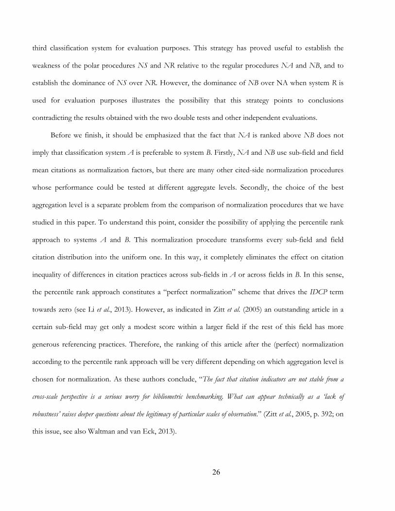
third classification system for evaluation purposes. This strategy has proved useful to establish the

weakness of the polar procedures NS and NR relative to the regular procedures NA and NB, and to

establish the dominance of NS over NR. However, the dominance of NB over NA when system R is

used for evaluation purposes illustrates the possibility that this strategy points to conclusions

contradicting the results obtained with the two double tests and other independent evaluations.

Before we finish, it should be emphasized that the fact that NA is ranked above NB does not

imply that classification system A is preferable to system B. Firstly, NA and NB use sub-field and field

mean citations as normalization factors, but there are many other cited-side normalization procedures

whose performance could be tested at different aggregate levels. Secondly, the choice of the best

aggregation level is a separate problem from the comparison of normalization procedures that we have

studied in this paper. To understand this point, consider the possibility of applying the percentile rank

approach to systems A and B. This normalization procedure transforms every sub-field and field

citation distribution into the uniform one. In this way, it completely eliminates the effect on citation

inequality of differences in citation practices across sub-fields in A or across fields in B. In this sense,

the percentile rank approach constitutes a “perfect normalization” scheme that drives the IDCP term

towards zero (see Li et al., 2013). However, as indicated in Zitt et al. (2005) an outstanding article in a

certain sub-field may get only a modest score within a larger field if the rest of this field has more

generous referencing practices. Therefore, the ranking of this article after the (perfect) normalization

according to the percentile rank approach will be very different depending on which aggregation level is

chosen for normalization. As these authors conclude, “The fact that citation indicators are not stable from a

cross-scale perspective is a serious worry for bibliometric benchmarking. What can appear technically as a ‘lack of

robustness’ raises deeper questions about the legitimacy of particular scales of observation.” (Zitt et al., 2005, p. 392; on

this issue, see also Waltman and van Eck, 2013).

27

We would like to add that, once the question of the best aggregate level is somewhat settled, it

will be interesting to compare less than perfect classification-based-systems normalization procedures at

this and higher aggregate levels using the methods developed in this paper. Nevertheless, we should

conclude recognizing that more empirical work is needed before these methods become well

established. In particular, it will be illuminating to use other classification systems with interesting

properties of their own apart from the two polar cases studied here.

28

REFERENCES

Albarrán, P., J. Crespo, I. Ortuño, and J. Ruiz-Castillo (2011), “The Skewness of Science In 219 Sub-fields and a Number of Aggregates”, Scientometrics, 88: 385-397. Bornmann L. & Marx, W. (2013), “How good is research really?”, EMBO reports, 14: 226-230.

Boyack, K., R. Klavans, and K. Börner (2005), “Mapping the backbone of Science”, Scientometrics, 64: 351-374. Braun, T., W. Glänzel, & A. Schubert (1985), “Scientometrics Indicators. A 32 Country Comparison of Publication Productivity and Citation Impact”, World Scientific Publishing Co. Pte. Ltd., Singapore, Philadelphia.

Crespo, J. A., Li, Yunrong, and Ruiz-Castillo, J. (2013a), “The Measurement of the Effect On Citation Inequality of Differences In Citation Practices Across Scientific Fields”, PLoS ONE 8(3): e58727.

Crespo, J. A., Herranz, N., Li, Yunrong, and Ruiz-Castillo, J. (2013b), “The Effect on Citation Inequality of Differences in Citation Practices at the Web of Science Subject category Level”, Working Paper 13-03, Universidad Carlos III (http://hdl.handle.net/10016/16327), forthcoming in Journal of the American Society for Information Science and Technology.

Glänzel, W. (2011), “The Application of Characteristic Scores and Scales to the Evaluation and Ranking of Scientific Journals”, Journal of Information Science, 37: 40-48.

Glänzel, W. and A. Schubert (2003), “A new classification scheme of science fields and subfields designed for scientometric evaluation purposes”, Scientometrics, 56: 357-367.

Leydesdorff, L. (2004), “Top-down Decomposition of the Journal Citation Report of the Social Science Citation Index: Graph- and Factor Analytical Approaches”, Scientometrics, 60: 159-180.

Leydesdorff, L. (2006), “Can Scientific Journals Be Classified in Terms of Aggregated Journal-Journal Citation Relations Using the Journal Citation Reports?”, Journal of the American Society for Information Science and Technology, 57: 601-613.

Leydesdorff, L. and I. Rafols (2009), “A Global Map of Science Based on the ISI Categories”, Journal of the American Society for Information Science and Technology, 60: 348-362.

Leydesdorff, L., and Opthof, T. (2010), “Normalization at the Field level: Fractional Counting of Citations”, Journal of Informetrics, 4: 644-646.

Li, Y., Castellano, C., Radicchi, F., and Ruiz-Castillo, J. (2013), “Quantitative Evaluation of Alternative Field Normalization Procedures”, Journal of Informetrics, 7: 746– 755.  Moed H. F. (2010), “Measuring contextual citation impact of scientific journals”, Journal of Informetrics, 4: 265–77.

Moed, H. F., Burger, W.J. Frankfort, J.G., & van Raan, A.F.J. (1985) The Use of Bibliometric Data for the Measurement of University Research Performance. Research Policy, 14, 131-149.

Moed, H. F., & van Raan, AF.J. (1988) Indicators of Research Performance. in A. F. J. van Raan (ed.), Handbook of Quantitative Studies of Science and Technology, North Holland: 177-192.

Moed, H. F., De Bruin, R.E, & van Leeuwen, T. (1995) New Bibliometrics Tools for the Assessment of national Research Performance: Database Description, Overview of Indicators, and First Applications. Scientometrics, 33, 381-422.

Radicchi, F., Fortunato, S., & Castellano, C. (2008), “Universality of citation distributions: Toward an objective measure of scientific impact”, Proceedings of the National Academy of Sciences, 105: 17268–17272. Radicchi, F., and Castellano, C. (2012), “A Reverse Engineering Approach to the Suppression of Citation Biases Reveals Universal Properties of Citation Distributions”, PLoS ONE, 7, e33833, 1-7.

29

Schubert, A., & Braun, T. (1996), “Cross-field Normalization of Scientometric Indicators”, Scientometrics, 36: 311-324.

Schubert, A., Glänzel, W., Braun, T. (1983), “Relative Citation Rate: A New Indicator for Measuring the Impact of Publications”, in D. Tomov and L. Dimitrova (eds.), Proceedings of the First National Conference with International Participation in Scientometrics and Linguistics of Scientific Text, Varna.

Schubert, A., Glänzel, W., & Braun, T. (1987), “A New Methodology for Ranking Scientific Institutions”, Scientometrics, 12: 267-292.

Schubert, A., Glänzel, W., & Braun, T. (1988), “Against Absolute Methods: Relative Scientometric Indicators and Relational Charts as Evaluation Tools”, in A. F. J. van Raan (ed.), Handbook of Quantitative Studies of Science and Technology: 137-176.

Sirtes, D. (2012), “Finding the Easter Eggs Hidden by Oneself: Why Radicchi and Castellano’s (2012) fairness test for citation indicators is not fair”, Journal of Informetrics, 6: 448– 450. Small H, Sweeney E (1985) , “Clustering of science citation index using co-citations”, Scientometrics, 7: 393-404. Tijssen, J. W., and T. van Leeuwen (2003), “Bibliometric Analysis of World Science”, Extended Technical Annex to Chapter 5 of the Third European Report on Science and Technology Indicators, Directorate-General for Research. Luxembourg: Office for Official Publications of the European Community.

Vinkler, P. (1986) Evaluation of Some Methods For the Relative Assessment of Scientific Publications. Scientometrics, 10, 157-177.

Vinkler, P. (2003) Relations of Relative Scientometric Indicators. Scientometrics, 58, 687-694.

Waltman, L., & Van Eck, N. J. (2012a), “Source normalized indicators of citation impact: An overview of different approaches and an empirical comparison”, in press, Scientometrics. arXiv:1208.6122.

Waltman, L., & Van Eck, N.J. (2012b), “A new methodology for constructing a publication-level classification system of science”, Journal of the American Society for Information Science and Technology, 63: 2378-2392.

Waltman, L., and Van Eck, N. J. (2013), “A systematic empirical comparison of different approaches for normalizing citation impact indicators”, mimeo, Centre for Science and Technology Studies, Leiden University (arXiv:1301.4941). Zitt M., Ramana-Rahari, S., and Bassecoulard, E. (2005), “Relativity of Citation Performance and Excellence Measures: From Cross-field to Cross-scale Effects of Field-Normalization”, Scientometrics, 63: 373-401. Zitt M., and Small H. (2008), “Modifying the journal impact factor by fractional citation weighting: The audience factor”, Journal of the American Society for Information Science and Technology, 59: 1856-1860.    

30

APPENDIX

IDCPNK Term and Overall Citation Inequality I1(CK*) After Normalization By the Different Procedures

Classification System Used For Evaluation Purposes:

Normalization S A B R

Procedures

IDCPNK(S) I1(CK*) IDCPNK(A) I1(CK*) IDCPNK(B) I1(CK*) IDCPNK(A) I1(CK*)

(1) (2) (3) (4) (5) (6) (7) (8)

NS 0.2167 0.2173 0.1032 0.2173 0.0798 0.2173 0.0097 0.2173

NA 0.6385 0.7531 0.0260 0.7531 0.0122 0.7531 0.0076 0.7531

NB 0.6996 0.7876 0.0620 0.7876 0.0131 0.7876 0.0062 0.7876

NR 0.8628 0.8633 0.1678 0.8633 0.1143 0.8633 0.0021 0.8633

-------------------------------------------------------------------------------------------------------------------------------------------------------------------

IDCPNK(G) = citation inequality attributable to differences in citation practices across the disciplines in classification system G after

normalization by procedure NK, where K, G = S, A, B, and R

I1(CK*) = citation inequality in the all-sciences case after normalization by procedure NK, where K = S, A, B, and R

______________________________________________________________________________________________________

31

Table 1. The Effect on Citation Inequality of Differences in Citation Practices at the Sub-field and Field Levels

When the Raw Data Is Organized According to Four Classification Systems

Overall

IDCP Citation

Term Inequality (1)/(2) in %

CLASSIFICATION SYSTEMS (1) (2) (3)

S 0.8642 0.8644 99.98

A 0.1552 0.8644 17.95

B 0.1079 0.8644 12.48

R 0.0024 0.8644 0.28

------------------------------------------------------------------------------------------------------------------------------------------

System S = Systematic assignment at the sub-field level

System A = Articles classified into the 219 sub-fields corresponding to the Web of Science subject-categories

(fractional approach)

System B = Articles classified into 19 broad fields according to the aggregation scheme developed in

Albarrán e t a l . (2011)

System R = Random assignment at the sub-field level

_____________________________________________________________________________________________

32

 

Figure 1. The comparison of normalization procedures NS and NA using classification system A for evaluation purposes (quantile interval [548, 995])

0,0000  

0,0200  

0,0400  

0,0600  

0,0800  

0,1000  

0,1200  

0,1400  

0,1600  

0,1800  

0,2000  

548  

568  

588  

608  

628  

648  

668  

688  

708  

728  

748  

768  

788  

808  

828  

848  

868  

888  

908  

928  

948  

968  

988  

Evaluation system: A

Raw  data  

NA  

NS  

I1 (mπ)  

π

33

 

Figure 2. The comparison of normalization procedures NA and NB using classification system B for evaluation purposes (quantile interval [532, 999])

0,0000  

0,0200  

0,0400  

0,0600  

0,0800  

0,1000  

0,1200  

0,1400  

574  

599  

624  

649  

674  

699  

724  

749  

774  

799  

824  

849  

874  

899  

924  

949  

974  

999  

Evaluation system: B

Raw  data  

NA  

NB  

I1 (mπ)  

π

34

Table 2. The Impact of Normalization under the Four Classification Systems

Change in the Value of the IDCP Term after Normalization by the Different Procedures, in %

Normalization Classification System Used for Evaluation Purposes:

Procedures S A B R

(1) (2) (3) (4)

NS 74.9 33.5 26.0 - 304.7

NA 26.4 83.2 88.7 - 216.3

NB 19.4 60.1 87.8 - 158.6

NR 0.2 - 8.1 - 5.9 11.0

________________________________________________________________________________________________

35

             

Figure 3. The comparison of normalization procedures NS and NA using classification system S for evaluation purposes (quantile interval [523, 999])

0,0000  

0,2000  

0,4000  

0,6000  

0,8000  

1,0000  

1,2000  

1,4000  

523  

543  

563  

583  

603  

623  

643  

663  

683  

703  

723  

743  

763  

783  

803  

823  

843  

863  

883  

903  

923  

943  

963  

983  

Evaluation system: S    

Raw  data  

NA  

NS  

I1 (mπ)  

π

36

 

Figure 4. The comparison of normalization procedures NA and NB using classification system A for evaluation purposes (quantile interval [548, 995])

0,0000  

0,0200  

0,0400  

0,0600  

0,0800  

0,1000  

0,1200  

0,1400  

0,1600  

0,1800  

0,2000  548  

573  

598  

623  

648  

673  

698  

723  

748  

773  

798  

823  

848  

873  

898  

923  

948  

973  

Evaluation system: A

Raw  data  

NA  

NB  

I1 (mπ)  

π

37

 

Figure 5. The comparison of normalization procedures NA and NR using classification system A for evaluation purposes (quantile interval [548, 995])

0,0000  

0,0200  

0,0400  

0,0600  

0,0800  

0,1000  

0,1200  

0,1400  

0,1600  

0,1800  

0,2000  

548  

568  

588  

608  

628  

648  

668  

688  

708  

728  

748  

768  

788  

808  

828  

848  

868  

888  

908  

928  

948  

968  

988  

Evaluation system: A

NA  

NR  

I1 (mπ)  

π

38

 

Figure 6. The comparison of normalization procedures NA and NR using classification system R for evaluation purposes (quantile interval [604, 997])

0,0000  

0,0010  

0,0020  

0,0030  

0,0040  

0,0050  

0,0060  

0,0070  

0,0080  

0,0090  

0,0100  

604  

624  

644  

664  

684  

704  

724  

744  

764  

784  

804  

824  

844  

864  

884  

904  

924  

944  

964  

984  

Evaluation system: R

Raw  data  

NA  

NR  

I1 (mπ)  

π

39

 

Figure 7. The comparison of normalization procedures NA and NR using classification system S for evaluation purposes (quantile interval [500, 999])

0,0000  

0,2000  

0,4000  

0,6000  

0,8000  

1,0000  

1,2000  

1,4000  

500  

525  

550  

575  

600  

625  

650  

675  

700  

725  

750  

775  

800  

825  

850  

875  

900  

925  

950  

975  

Evaluation system: S

NA  

NR  

I1 (mπ)  

π

40

Figure 8. The comparison of normalization procedures NA and NB using classification system R for evaluation purposes (quantile interval [608, 996])

0,0000  

0,0010  

0,0020  

0,0030  

0,0040  

0,0050  

0,0060  

0,0070  

0,0080  

0,0090  

0,0100  

608  

633  

658  

683  

708  

733  

758  

783  

808  

833  

858  

883  

908  

933  

958  

983  

Evaluation system: R

Raw  data  

NA  

NB  

I1 (mπ)  

π