IZA DP No. 480

The Complexity of Economic Policy:I. Restricted Local Optima in Tax Policy Design

Gilles Saint-Paul

DI

SC

US

SI

ON

PA

PE

R S

ER

IE

S

Forschungsinstitutzur Zukunft der ArbeitInstitute for the Studyof Labor

April 2002

The Complexity of Economic Policy: I. Restricted Local Optima in Tax Policy Design

Gilles Saint-Paul GREMAQ-LEERNA-IDEI,

Université des Sciences Sociales de Toulouse and IZA, Bonn

Discussion Paper No. 480 April 2002

IZA

P.O. Box 7240 D-53072 Bonn

Germany

Tel.: +49-228-3894-0 Fax: +49-228-3894-210

Email: iza@iza.org

This Discussion Paper is issued within the framework of IZA’s research area Evaluation of Labor Market Policies and Projects. Any opinions expressed here are those of the author(s) and not those of the institute. Research disseminated by IZA may include views on policy, but the institute itself takes no institutional policy positions. The Institute for the Study of Labor (IZA) in Bonn is a local and virtual international research center and a place of communication between science, politics and business. IZA is an independent, nonprofit limited liability company (Gesellschaft mit beschränkter Haftung) supported by the Deutsche Post AG. The center is associated with the University of Bonn and offers a stimulating research environment through its research networks, research support, and visitors and doctoral programs. IZA engages in (i) original and internationally competitive research in all fields of labor economics, (ii) development of policy concepts, and (iii) dissemination of research results and concepts to the interested public. The current research program deals with (1) mobility and flexibility of labor, (2) internationalization of labor markets, (3) welfare state and labor markets, (4) labor markets in transition countries, (5) the future of labor, (6) evaluation of labor market policies and projects and (7) general labor economics. IZA Discussion Papers often represent preliminary work and are circulated to encourage discussion. Citation of such a paper should account for its provisional character. A revised version may be available on the IZA website (www.iza.org) or directly from the author.

IZA Discussion Paper No. 480 April 2002

ABSTRACT

The Complexity of Economic Policy: I. Restricted Local Optima in Tax Policy Design

Economists traditionally tackle normative problems by computing optimal policy, i.e. the one that maximizes a social welfare function. In practice, however, a succession of marginal changes to a limited number of policy instruments are implemented, until no further improvement is feasible. I call such an outcome a ”restricted local optimum”. I consider the outcome of such a tatonnement process for a government which wants to optimally set taxes given a tax code with a fixed number of brackets. I show that there is history dependence, in that several local optima may be reached, and which one is reached depends on initial conditions. History dependence is stronger (i.e. there are more local optima), the more complex the design of economic policy, i.e. the greater the number of tax brackets. It is also typically stronger, the greater the interaction of policy instruments with one another – which in my model is equivalent to agents having a more elastic labor supply behavior. Finally, for a given economy and a given tax code, I define the latter’s average performance as the average value of the social welfare function across all the local optima. One finds that it eventually sharply falls with the number of brackets, so that the best performing tax code typically involves no more than three brackets. JEL Classification: H2, H21, J22 Keywords: complexity, optimal taxation, bounded rationality, learning, multiple equilibria,

path dependence Gilles Saint-Paul IDEI, Université des Sciences Sociales Manufacture des Tabacs Allée de Brienne 31000 Toulouse France Tel.: (33) 5 61 12 85 44 Fax: (33) 5 61 22 55 63 Email: gilles.saint-paul@univ-tlse1.fr

1 Introduction

Economists traditionally tackle normative problems by computing optimal

policy, i.e. the one that maximizes a social welfare function. In practice, how-

ever, the actual conduct of economic policy rarely follows these guidelines.

The whole set of government interventions–taxes, subsidies, and regulations–

is characterized by a large set of parameters and, even if one were given an

appropriate social welfare function, it is impossible to compute their optimal

values. Rather, reform takes place as follows. There is status quo de…ned

by a set of policy parameters inherited from the past, and there is a social

demand to alter this status quo. Government respond to this status quo

by altering a small subset of parameters, often marginally, i.e. by a small

amount. The status quo gradually evolves as a result of this trial-and-error

process. We expect the process to stop when no such marginal improvements

are feasible.

Thus, rather than a …rst-best optimal policy being selected, the economy

converges to a local optimum in a restricted sense, i.e. in the sense that the

objective function cannot be improved by a small change to a small subset

of parameters.

This raises a number of questions which do not arise in traditional optimal

policy analysis. For example:

² To what extent is the resulting policy history-dependent? In a …rst best

world, the optimum will be selected regardless of initial conditions.

Under my trial and error assumption, if there are several restricted

local optima, which one will eventually be selected will depend on initial

conditions. The greater the number of local optima, the more arbitrary

and history-dependent the policy outcome.

² How large are the losses that history-dependence may cause? In other

words, do all local optima yield comparable values for the objective

function, or are some of them clearly worse that others?

2

² Should economic policy be simple or complex, that is, how many in-

struments should we use? In a …rst best world, an increase in the

number of instruments is always bene…cial, because it increases the set

of policies that can be pursued (simple policies can always be replicated

when more instruments are introduced). This is not necessarily true,

however, in a trial-and-error world. Having more instruments could in

principle increase the number of restricted local optima in such a way

that some of them are worse than local optima under simpler policies.

In other words, if complexity increases the number of local optima, it

may make policy more history-dependent. This increases the likelihood

of being remote from the best policy, i.e. makes large bene…cial policy

changes less likely to occur. In such a situation, one may make a case

for simpler policies.

I analyze these issues in the context of a model of optimal taxation. The

underlying structure of preferences and technology is standard. Agents di¤er

in their ability as well as in their disutility of working. Income is taxed

and the tax code is piece-wise linear, being characterized by n tax brackets.

Tax proceeds are used to …nance a public good. The social welfare function

depends on the level of the public good as well as on a composite index of

income which re‡ects a concern about inequality. The only tax policy changes

that are allowed are those which move one critical point in the tax schedule up

or down by a small …xed amount. I call this a ”feasible reform”. A restricted

local optimum (RLO) is reached when no feasible reform improves social

welfare. I compute these local optima by starting from randomly selected tax

codes, and then sequentially implementing feasible reforms, until an RLO is

reached.

Our numerical results suggest that the number of RLOs goes up with

the complexity of the tax system, as captured by the number of brackets.

It also typically goes up when the curvature of the disutility of labor goes

up, i.e. when labor supply is more reactive to changes in marginal tax rates.

Another striking implication is that an increase in complexity beyond a cer-

3

tain level is harmful to the expected performance of the tax system. That

is, while greater complexity allows to better ’…ne-tune’ the best optimum,

thus improving the corresponding value of the social welfare function, it also

introduces new RLOs whose performance can be quite poor. I de…ne the

performance of the tax system as the average social level across RLOs, when

each RLOs is weighted by the frequency with which is was reached across

searches. When the number of tax brackets goes up beyond some point,

performance deteriorates, implying that the welfare loss from reaching sub-

optimal equilibria more often outweigh the welfare gains from improving the

value of the best optimum.

Our results are similar to those found by Kau¤man (1985) in his so-called

NK model. This is an abstract statistical model which the author uses

to analyze the evolution of complex biological objects such as proteins or

DNA. A somewhat similar approach has been applied by Durlauf (1993) and

Brock and Durlauf (2001) to economic problems such as ghetto formation

and multiple long-run growth paths. The essence of these results is that

path-dependence is more likely, the greater the complexity of the system and

the greater the degree of interaction among units. Speci…cally, Kau¤man

considers N units who can be in one of two boolean states (0 or 1), and

whose individual contribution to the overall …tness of the system depends on

the state of K other units. By running numerous numerical simulations over

randomly de…ned such systems characterized by K and N; Kau¤man shows

that the ”…tness landscape”, i.e. the way the objective function varies over

di¤erent states of the system, is more ”rugged”, i.e. has more local optima,

the greater K and N:

In my model, the equivalent of a unit is a given tax bracket, and the inter-

action among tax brackets is larger, the smaller the curvature of the disutility

of e¤ort. If this curvature is very strong, then labor supply is very inelastic

to marginal income taxes, and so is income. The contribution of a given tax

bracket to overall inequality and tax receipts is then basically independent of

the level of other tax brackets, since workers have little opportunity to change

4

tax brackets by changing their e¤ort level. By contrast, if labor supply is

very elastic, a change in a given tax bracket can induce a strong realloca-

tion of workers among tax brackets. Thus interaction among tax brackets

is stronger, the more elastic is labor supply. Finally, the equivalent of the

biologist’s …tness function is the social welfare function.

The similarity of our results with those of Kau¤man are suggestive, but

the present model is not a special case of his NK model. While Kau¤man

considers any arbitrary, randomly generated, function de…ning the contribu-

tion of each unit to total …tness, in my model total …tness is the result of the

underlying economic behavior of optimizing economic agents.

2 The economy

The arti…cial economies I consider have a standard structure. There are q

agents, who have access to a constant returns to scale technology producing

a single homogeneous good using labor. Agents di¤er by their ability and

their disutility of e¤ort. Utility is given by

U (c; e) = c¡ be´=´;

where c is consumption, e is e¤ort, b is the individual speci…c parameter

capturing di¤erences in the disutility of labor, and ´ is a parameter capturing

the curvature of this disutility. The greater ´; the more inelastic is labor

supply. As ´ goes to in…nity, labor supply becomes totally inelastic as each

agent supplies one unit of e¤ort.

The amount of good produced by an agent with ability a is

y = ae;

where e is the agent’s e¤ort level. For simplicity, I assume that e¤ort cannot

exceed 1=a; so that total income is between 0 and 1.

The tax code is a function relating net income z to gross income y :

z = z(y):

5

I assume that the tax code is continuous and piece wise linear over n

intervals, called ‘brackets’, whose n+1 kink points are equidistant; I restrict

net income to be also between 0 and 1. A typical tax code is illustrated in

Figure 1. Decreasing portions, i.e. portions with a marginal tax rate greater

than 100 %, are ruled out.1

The consumers’ budget constraint implies z(y) = c: Therefore, their op-

timum e¤ort level is given by:

e = e¤(a; b) = arg maxe2[0;1=a]

z(y)¡ be´=´

The government tries to maximize an objective function which re‡ects

a concern for income distribution, as well as to provide for a public good.

Speci…cally I assume that the social welfare function is given by

W =

24Ã1

q

qX

i=1

z(yi)°

!Ã=°

+ ¸

µT

q

¶Ã351=Ã

;

where T is net total tax receipts:

T =

qX

i=1

yi ¡ z(yi):

The social welfare function is therefore a CES aggregate of total tax

receipts per capita, and of an index of average personal disposable income

adjusted for inequality in the fashion of Atkinson (1970).2 This index is

homogeneous of degree one in disposable income, but increases with mean-

preserving redistributions. Concern for inequality is captured by ° · 1:

1There is no a priori problem with having such portions, except that allowing themtends to spuriously increase the number of local optima. This is because marginal taxrates in excess of 100 % may generate con…gurations where disposable income falls withpre-tax income beyond a certain income level. Nobody would get a pre-tax income greaterthan this threshold, and marginal changes in the tax code in this zone typically have noe¤ect. This tends to generate a large number of equivalent local optima. To rule out thispossibility we impose that marginal tax rates should not exceed 100 %.

2Note that the (unobservable) disutility of labor is not taken into account in the socialwelfare function.

6

The smaller °; the greater inequality aversion. T=q enters because net tax

receipts are spent on a public good. ¸ and à capture the relative weight of the

public good in social welfare and the social elasticity of substitution between

(inequality adjusted) disposable income and the public good, respectively.

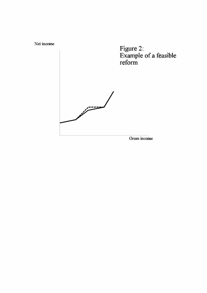
Starting from a given tax code, the government tries to improve it by

implementing a succession of small restricted changes to the tax code. It

can only move net income by §0:005 at one kink point at a time. Figure 2

gives an example of a feasible tax changes. If no such tax change improves

social welfare, then we have a restricted local optimum, which we consider

as a potential equilibrium outcome of the economy.

The next section describes in detail the procedure which was followed in

order to compute these RLOs.

3 Procedure

An economy is randomly generated with q agents. For each agent, a is drawn

over [0; 1]; and b is independently drawn over [1; 2]; using a uniform distri-

bution in both cases. The policymaker starts from a randomly determined

tax code with n brackets, by randomly selecting disposable income at each

of the kink points, subject to the constraint that marginal tax rates cannot

exceed 100 %.

Given a tax code, I compute the e¤ort level of each individual by a grid

search over [0; 1=a]:3 This allows to compute aggregates such as GDP, tax

receipts, and social welfare. If the initial, randomly drawn tax code yields

negative tax receipts, another one is drawn, until one ends up with a revenue-

generating scheme.

Then a restricted local optimum is reached by the following iteration

procedure: a number m is randomly selected, and z(m=n); i.e. disposable

income that the kink point between bracketm and bracketm+1; is increased

by 0.005, as described in the previous section. Social welfare using this new

3The step which was used was 0.01.

7

tax code is computed and compared to its value under the previous tax code.

If an improvement is obtained, then the new tax code is substituted for the

old one, and the procedure is repeated. Otherwise, one decreases z(m=n)

by 0.005. If no improvement is obtained, the procedure considers similar

changes for other possible kink points, in the following order: (m+1)=n; (m+

2)=n; :::; 1; 0; 1=n; :::; (m¡ 1)=n: As soon as an improvement is obtained, the

new tax code replaces the old one and the procedure is repeated. If no

improvement is obtained for all possible kink points, one has reached an

RLO and the procedure stops.

For each set of parameter values, I have generated 10 di¤erent random

economies. For each of them, I have considered all the values of n between

n = 1 and n = 6: Given an economy and a value of n; the search for a

local optimum is repeated 15n times, starting from 15n di¤erent randomly

generated initial tax codes.4

Given computational errors, from a strictly numerical perspective the

15n searches are likely to yield 15n di¤erent outcomes. One can then in

principle look at all these tax codes and consider those which are ”close”

as the same RLO. However, this is time consuming and not very precise.

In order to give a precise content to such an ”optical” method, I use the

following kernel transformation. For k = 1; :::; 15n; the corresponding RLO

is a vector Xk 2 [0; 1]n+1: For any vector X the kernel function is then given

by:

K(X) =15nX

k=1

1

¾exp(¡kX ¡Xkk2

2¾2):

I then use the local optima of K(X) as my estimates of local optima.5

4In order to preserve the relative density of initial tax codes in the tax code space as ngoes up, one would need to have the number of searches to increase like xn: However, thisis exteremly costly in terms of computer time, so we have chosen a more modest option.Intuitively, it implies that one is more likely to miss some local optima as n goes up, thusleading us to underestimate the e¤ect of n on the number of local optima.

5To compute these local optima, we use the actual values of Xk as starting point foran iteration procedure using the Newton-Raphson method. This makes sense since the

8

The precision of this method is captured by ¾: If ¾ is very small, there

will be as many humps as values of Xk: If ¾ is very large, K(:) is very

smooth and has very few humps. After various experimentations I have used

¾ = 0:03pn+ 1:6

4 Results

Table 1 reports the average number of restricted local optima found by the

procedure. Each number is the average over 10 randomly selected economies.

The key …nding which emerges from Table 1 is that the number of RLOs

typically raises sharply with the number of tax brackets n; while it is low for

a single tax bracket. Therefore, economies with more complex tax systems

are more likely to be stuck at a history-dependent, ine¢cient local RLO.

However, this ceases to be true at very high elasticities of labor supply. For

´ = 1:5; the number of local optima goes up with the number of brackets,

but then it falls.

Furthermore, the number of optima …rst increases and then falls with the

elasticity of labor supply 1=(´¡1): Thus, for n = 3; for example, the average

number of optima increases from 2.4 to 6.2 as ´ falls from 10 to 2, but it then

falls to 4.0 as ´ falls to 1.5.

How could one explain such nonmonotonicity? When ´ goes down, the

e¤ect of a local reform is more complex, because people are more likely to

move across brackets. Kau¤man’s …ndings suggest that this should increase

the number of optima as the objective function becomes more ‘rugged’ in the

policy space. This is indeed what I …nd except for the lowest value of ´: As

´ falls, an increasing proportion of agents elect a corner solution (e = 0 or

e = 1=a) for their e¤ort level. This tends to reduce the e¤ective response of

local optima should be ‘close’ to the computed ones. If two initial values of Xk lead totwo estimated local optima for K(X) such that the Euclidian distance between them islower than ¾=3; then they are considered as the same local optimum.

6Proportionality between ¾2 and the dimension of the relevant space guarantees thatas n goes up, the average ‘tolerance’ per kink point is kept constant.

9

e¤ort levels to marginal changes in the tax code. In other words, the true

elasticity of labor supply does not necessarily fall when ´ becomes small. It

falls for agents who are not at a corner solution but on the other hands more

agents are at a corner solution. Thus, that the number of optima eventually

falls as ´ reaches 1.5 does not necessarily contradict our basic intuition.

nn´ 10 5 2 1.51 1 (0.0) 1 (0.0) 2.0 (0.2) 2.0 (0.1)2 2.2 (0.2) 3.7 (0.3) 4.1 (0.3) 2.7 (0.3)3 2.4 (0.4) 4.9 (0.4) 6.2 (0.3) 4.0 (0.4)4 2.6 (0.3) 4.5 (0.4) 8.7 (0.4) 6.7 (0.7)5 3.0 (0.5) 4.2 (0.25) 8.7 (0.4) 5.5 (0.4)6 3.9 (0.4) 5.3 (0.4) 10.3 (0.7) 4.1 (0.5)

Table 1 – Number of optima as a function of n and ´:

Table 2 reports how the complexity of the tax system a¤ects its average

performance. This average performance is de…ned as the average value, de-

noted by W (n), of the social welfare function over all 15n searches for RLOs

that were made for a given economy. In other words, it is a weighted av-

erage of the objective function across local optima, where each optimum is

weighted by the frequency with which it was reached. For any economy I

then compute the relative performance of the tax system with n brackets as

R(n) = W (n)=W (1); the ratio between the average performance at n and

the average performance with 1 brackets. Table 2 then reports the average

value of R(n) across the 10 randomly generated economies.

The results in Table 2 are striking. For ´ = 2; 5; and 10; performance

quickly falls when the number of tax brackets becomes too large. That is,

the extra losses from being trapped at new, ine¢cient optima which did not

exist for more simple tax systems outweigh the extra gains from a better

…ne-tuning of tax policy. Furthermore, this e¤ect is stronger, the lower ´;

i.e. the greater the e¤ect of an increase in n on the number of optima. For

example, an increase in the number of tax brackets from n = 1 to n = 6

reduces average performance by 5.4 % if ´ = 10; but it reduces it by 12.1 %

10

for ´ = 5 and by 23.2 % for ´ = 2: Consequently, optimal tax systems have

few brackets. The best performing value of n is 3 for ´ = 10; and 2 for ´ = 2

or ´ = 5:

The story is pretty di¤erent, however, when labor supply elasticity be-

comes very large. For ´ = 1:5; more complex tax systems always perform

better than n = 1: While the optimal number of brackets is n = 3; the loss

from increasing tax complexity beyond the optimum are smaller than in the

´ = 2 case (some 8 % instead of 23 %). One can speculate that these results

are again due to the fact that an increasing number of agents elect a corner

solution for e¤ort, thus being inelastic at the margin.

The results are in sharp contrast to what one would expect in a …rst best

world. In such a world, an increase in the number of tax brackets by an

integer multiplicative factor would always increase welfare, since the old tax

rates could be replicated using the new tax system.7 But this only holds if the

optimum optimorum is implemented. If instead equilibrium policy is de…ned

as an RLO reached by a tatonment procedure, then average performance can

go down because new ine¢cient RLOs are introduced when the tax system’s

complexity is increased.

nn´ 10 5 2 1.51 1.0 1.0 1.0 1.02 1.008 (0.003) 1.001 (0.006) 1.009 (0.015) 1.08 (0.013)3 1.01 (0.003) 0.976 (0.006) 0.925 (0.015) 1.09 (0.019)4 0.999 (0.004) 0.957 (0.009) 0.861 (0.015) 1.05 (0.026)5 0.972 (0.006) 0.913 (0.006) 0.81 (0.014) 1.04 (0.026)6 0.946 (0.006) 0.879 (0.01) 0.768 (0.019) 1.007 (0.033)

Table 2 – Average relative performance of tax systems.

Table 3 provides an example of the 4 policy outcomes that are found

for one of the economies with n = 3 and ´ = 5: For each local optimum,

7Note that in terms of the global optimum n = 3 does not necessarily dominate n = 2;since the kink points are pegged at 1=n; implying that one cannot typically replicate a taxcode with n = 2 with a 3-bracket tax code.

11

Columns 2 to 5 respectively report the value of the objective function, total

tax receipts, GDP, and the frequency with which the optimum is reached.

Column 6 gives the net income of an agent with zero pre-tax income, i.e. the

transfer made to the poorest. Columns 7 to 9 give the marginal tax rate in

each bracket, from the bottom to the top of the distribution of income.

The most frequently reached RLO (Equilibrium #1) is also the most

desirable one. It has the property that marginal tax rates fall when income

goes up, in accordance with the …ndings of Mirrlees (1971). In 26.6 % of the

cases, however, the economy converges to an equilibrium which is much more

redistributive, with a marginal tax rate of 100 % for top earners, and slightly

higher marginal tax rates than Equilibrium #1 for other agents. Tax receipts

are only slightly above their level in the other equilibrium, so that the transfer

to the poorest is only slightly larger. On the other hand, GDP is 12 % lower,

so that on net this equilibrium performs much worse than the other one.

Finally, there exists two other rare equilibria. The …rst one has substantially

higher tax receipts than the other two, at the cost of con…scatory tax rates

for bottom and low earners. It subsidizes high earnings at the margin, thus

inducing a high e¤ort level by many agents, but still extorts high taxes from

the wealthy, as the average tax rate is about 60 % for top earners. These

high distortions strongly reduce GDP, while there is little redistribution; but

tax receipts and thus the level of public goods is higher than in the other two

equilibria. Finally, Equilibrium #4 also virtually expropriates all low and

medium income workers, while giving strong work incentives at the top. It

has lower tax receipts than other equilibria, but a higher GDP than equilibria

#2 and #3.

Eqbm # V T Y F z(0) MTR1 MTR2 MTR31 .601 .14 .352 .683 .107 0.85 0.57 0.172 0.562 0.15 0.31 0.266 0.108 0.856 0.601 1.03 0.39 0.197 0.26 0.033 0.025 0.948 1.0 -0.134 0.24 0.138 0.326 0.017 0.01 0.985 0.999 -1.46

Table 3 – Characteristics of four RLOs in one of the simulated economies,

12

with n = 3 and ´ = 5:

As table 3 suggests, there exist local optima that perform very poorly,

although those in Table 3 tend to be quite infrequent. Table 4 computes

the maximum damage of history dependence as measured by the percentage

di¤erence between the value of the objective function at the best optimum

and its value at the worst one. As Table 4 shows, this loss can be huge and

tends to go up with the system’s complexity as well as labor supply elasticity,

with again an exception at very low elasticities.

nn´ 10 5 2 1.51 0 0 14.9 35.82 18.8 39.7 60.4 29.13 19.4 58.1 74.2 39.54 32 76.2 80.2 50.95 45.4 78.7 83.1 57.26 51.5 71.1 84.7 59.5

Table 4 – Maximum loss (%)

As this pattern may just be driven by very infrequent poor outcomes,

Table 5 looks at the average loss, i.e. at the di¤erence between the average

performance of searches and welfare at the best optimum. It con…rms that

losses can be quite large and are overall larger, the more complex the system

and the greater the elasticity of labor supply.

nn´ 10 5 2 1.51 0 0 5.9 11.22 1.4 4.6 9.0 7.53 1.9 6.7 20.5 10.74 3.2 9.5 27.0 15.75 6.1 13.4 31.7 18.36 8.7 17.1 34.9 22.2

Table 5 – Average loss (%)

13

5 Robustness checks

In order to check the robustness of my results, I have run a number of simu-

lations with di¤erent parameter values.8

First, I have allowed for lower inequality aversion by running simulations

with ° = ¡1 and ° = ¡0:5 instead of ° = ¡2: The results are quite similar to

the ones reported above (see Appendix), with the exception that the number

of optima does not systematically rise monotonically with n for ´ = 2; 5; 10:

In some cases, it slightly falls for n ¸ 4; although this is often not signi…cant.

All the other patterns are con…rmed, in particular the ”optimal” number of

brackets never exceeds 3.

Second, I have changed the parameter à which captures the degree of

complementarity between public expenditure and inequality-adjusted GDP

in the social welfare function, by trying à = ¡0:5 instead of à = 0:5: Results

are again similar.

Finally, I have tried with other weights of public expenditure in the social

welfare function (¸ = 2 and ¸ = 0:5). Results are again similar.

6 Conclusion

Government policy is based on a large set of interventions: taxes, subsidies,

regulations, and discretionary interventions. This paper has explored the idea

that they cannot all be changed at the same time, and that the government

cannot compute its optimal mix. Rather, it can implement marginal reforms,

and keep them if they prove satisfactory.

In the context of tax policy, we have shown that this piece-meal, taton-

ment approach to economic policy may generate history dependence, in that

several local optima may be reached, and which one is reached depends on

initial conditions. History dependence is stronger (i.e. there are more local

8In these checks, 4 economies instead of 10 were used for each parameter set. Resultsare reported in the Appendix.

14

optima), the more complex the design of economic policy, and the greater the

interaction of policy instruments with one another–which in my tax model

means that economic agents have a more elastic behavior.

Furthermore, while a more complex policy design may in principle im-

prove outcomes because it increases the value of the best optimum, in practice

a complex system may have a lower performance. This is because complexity

increases the number of local optima, so the search process may more often

yield unsatisfactory outcomes, implying that welfare is lower on average. In-

deed, in the context of my tax model, the best performing number of tax

brackets is typically equal to 2 or 3.

In the future, I plan to apply similar analysis to other aspects of economic

policy, such as environmental regulation or active labor market policies, for

example.

15

REFERENCES

Atkinson, Anthony B. (1970) ”On the measurement of inequality”, Jour-

nal of Economic Theory, 2(3), 244-63

Brock, William and Steven Durlauf (2001), ”Discrete choice with local

interactions”, Review of Economic Studies, 68(2), 235-60

Durlauf, Steven (1993), ”Nonergodic economic growth”, Review of Eco-

nomic Studies 60(2), 349-66

Kau¤man, Stuart (1985), The Origins of Order, Oxford U. Press

Mirrlees, James (1971), ”An exploration in the theory of optimal taxa-

tion”, Review of Economic Studies, 38(114), 175-208

16

APPENDIX – Robustness checks

nn´ 10 5 2 1.51 1 (0.0) 1 (0.0) 1.25 (0.25) 2 (0)2 2 (0.0) 3.75 (0.5) 4.25 (0.25) 3.0 (0.4)3 2.75 (0.5) 6.0 (0.7) 7 (0.7) 5.25 (0.5)4 5.25 (0.75) 6.5 (0.6) 9.25 (0.5) 6.25 (0.9)5 4.5 (0.3) 5.25 (0.6) 8.75 (1.3) 5.5 (1.0)6 4.0 (0.7) 5 (0.0) 7.75 (0.5) 4 (0.7)

Table A1 – Number of optima as a function of n and ´; ° = ¡1

nn´ 10 5 2 1.51 1.0 1.0 1.0 1.02 1.003 0.99 0.96 1.063 1.009 0.98 0.84 0.994 0.99 0.92 0.79 0.955 0.97 0.9 0.7 0.876 0.95 0.85 0.69 0.83

Table A2 – Average relative performance of tax systems;° = ¡1

nn´ 10 5 2 1.51 1 (0.0) 1 (0.0) 2 (0.0) 2.5 (0.3)2 1.5 (0.3) 3.5 (0.3) 4.0 (0.4) 3.25 (0.5)3 3.5 (0.9) 4.0 (0.7) 7.25 (0.6) 5.75 (0.6)4 4.5 (0.6) 5.25 (0.9) 9.5 (0.3) 7.75 (1.0)5 5.0 (0.7) 6.25 (1.25) 10 (0.9) 5.25 (1.1)6 4.25 (0.6) 5.25 (0.6) 10.25 (1.6) 6.75 (0.8)

Table A3 – Number of optima as a function of n and ´; ° = ¡0:5

nn´ 10 5 2 1.51 1.0 1.0 1.0 1.02 1.01 0.99 0.99 1.083 0.999 0.96 0.85 1.094 0.987 0.92 0.79 1.0165 0.973 0.86 0.74 0.996 0.96 0.86 0.7 0.94

Table A4 – Average relative performance of tax systems;° = ¡0:5

17

nn´ 10 5 2 1.51 1 (0.0) 1.25 (0.25) 1.5 (0.3) 2.75 (0.25)2 2.5 (0.5) 3.5 (0.6) 3.5 (0.3) 2.75 (0.25)3 2.75 (0.5) 3 (1.1) 7 (0.6) 5 (0.7)4 3.25 (0.5) 5.5 (0.6) 9.25 (0.6) 6.25 (0.8)5 2.75 (0.25) 5.25 (0.9) 8.5 (1.2) 5.25 (0.8)6 4.25 (1.2) 5.5 (0.9) 9 (1.3) 5.75 (1.3)

Table A5 – Number of optima as a function of n and ´;Ã = ¡0:5

nn´ 10 5 2 1.51 1 1 1 12 1.002 1.017 0.95 1.223 1.007 1.007 0.89 1.234 0.983 0.93 0.84 1.1555 0.971 0.88 0.79 1.186 0.944 0.857 0.73 1.14

Table A6 – Average relative performance of tax systems;Ã = ¡0:5nn´ 10 5 2 1.51 1 (0.0) 1 (0.0) 1.5 (0.3) 2 (0.0)2 1.5 (0.3) 3.25 (0.5) 4 (0.4) 2.75 (0.25)3 1.75 (0.5) 3.0 (0.7) 6.75 (0.5) 5.5 (0.95)4 2.0 (0.4) 3.0 (0.7) 8.5 (0.9) 7.25 (0.75)5 2.75 (0.5) 3 (0.0) 8.0 (0.7) 6.25 (0.5)6 3.0 (0.4) 5.0 (0.4) 8.25 (1.8) 6.75 (1.0)

Table A7 – Number of optima as a function of n and ´;¸ = 2

nn´ 10 5 2 1.51 1 1 1 12 1.01 1.023 0.995 1.1353 1.015 1.01 0.936 1.0714 0.999 0.998 0.847 1.0375 0.999 0.987 0.806 1.0116 0.995 0.955 0.824 1.014

Table A8 – Average relative performance of tax systems;¸ = 2

18

nn´ 10 5 2 1.51 1 (0.0) 1 (0.0) 1.75 (0.25) 2.0 (0.41)2 1.25 (0.25) 3.75 (0.48) 4 (0.0) 2.75 (0.25)3 3.0 (0.41) 6.5 (0.29) 7.5 (0.96) 6.0 (0.58)4 5.5 (0.29) 7.25 (0.63) 9.0 (0.82) 8.25 (1.65)5 7.0 (0.41) 5.75 (0.25) 10.5 (2.18) 6.25 (1.18)6 5.25 (0.75) 7.5 (0.87) 9.0 (0.71) 7.25 (1.44)

Table A9 – Number of optima as a function of n and ´;¸ = 0:5

nn´ 10 5 2 1.51 1 1 1 12 1.016 0.969 0.925 1.063 0.998 0.958 0.836 1.024 0.963 0.879 0.733 0.9565 0.935 0.851 0.693 0.9156 0.865 0.794 0.659 0.899

Table A10 – Average relative performance of tax systems;¸ = 0:5

19

IZA Discussion Papers No.

Author(s) Title

Area Date

465 J. Ermisch M. Francesconi

Intergenerational Social Mobility and Assortative Mating in Britain

1 04/02

466 J. E. Askildsen E. Bratberg Ø. A. Nilsen

Unemployment, Labour Force Composition and Sickness Absence: A Panel Data Study

1 04/02

467 A. Venturini C. Villosio

Are Immigrants Competing with Natives in the Italian Labour Market? The Employment Effect

1 04/02

468 J. Wagner

The Impact of Risk Aversion, Role Models, and the Regional Milieu on the Transition from Unemployment to Self-Employment: Empirical Evidence for Germany

1 04/02

469 R. Lalive J. C. van Ours J. Zweimüller

The Effect of Benefit Sanctions on the Duration of Unemployment

3 04/02

470 A. Cigno F. C. Rosati L. Guarcello

Does Globalisation Increase Child Labour? 2 04/02

471 B. R. Chiswick Y. Liang Lee P. W. Miller

Immigrants’ Language Skills and Visa Category

1 04/02

472 R. Foellmi J. Zweimüller

Structural Change and the Kaldor Facts of Economic Growth

3 04/02

473 J. C. van Ours A pint a day raises a man’s pay, but smoking blows that gain away

5 04/02

474 J. T. Addison L. Bellmann A. Kölling

Unions, Works Councils and Plant Closings in Germany

3 04/02

475 Z. Hercowitz E. Yashiv

A Macroeconomic Experiment in Mass Immigration

1 04/02

476 W. A. Cornelius T. Tsuda

Labor Market Incorporation of Immigrants in Japan and the United States: A Comparative Analysis

1 04/02

477 M. A. Clark D. A. Jaeger

Natives, the Foreign-Born and High School Equivalents: New Evidence on the Returns to the GED

6 04/02

478 H. Gersbach A. Schniewind

Uneven Technical Progress and Unemployment

3 04/02

479 J. T. Addison C. R. Belfield

Unions and Employment Growth: The One Constant?

1 04/02

480 G. Saint-Paul

The Complexity of Economic Policy: I. Restricted Local Optima in Tax Policy Design

6 04/02

An updated list of IZA Discussion Papers is available on the center‘s homepage www.iza.org.