Embed Size (px)
Citation preview
WP/13/207
The Composition of Fiscal Consolidation Matters:
Policy Simulations for Hungary
Alejandro Guerson
© 2013 International Monetary Fund WP/13/207
IMF Working Paper
Fiscal Affairs Department
The Composition of Fiscal Consolidation Matters: Policy Simulations for Hungary
Prepared by Alejandro Guerson
Authorized for distribution by Abdelhak Senhadji
October 2013
Abstract
This paper evaluates policy alternatives to achieve permanent fiscal consolidation in
Hungary, based on a general equilibrium calibration. The main finding is that the
composition of the consolidation, as determined by the mix of revenue and expenditure
measures, has important implications for growth, employment, investment, and other key
macroeconomic variables. A reduction in current expenditures yields the smallest GDP
contraction in the short term and can increase output in the long term by stimulating labor
participation and private investment. On the other end of the spectrum, a consolidation of
government investment and corporate taxes are the most costly, as disincentives for
private investment result in protracted declines in GDP that compound over time to GDP
losses that are multiple times the initial size of the consolidation.
JEL Classification Numbers:E27, E62, H21, H30, H39, H50, H63
Keywords: fiscal consolidation, Hungary, DSGE models, overlapping generations households,
liquidity constrained households, financial accelerator, macro-financial linkages
Author’s E-Mail Address: [email protected]
This Working Paper should not be reported as representing the views of the IMF.
The views expressed in this Working Paper are those of the author(s) and do not necessarily
represent those of the IMF or IMF policy. Working Papers describe research in progress by the
author(s) and are published to elicit comments and to further debate.
2
Contents Page
Abstract ......................................................................................................................................1
I. Introduction ...................................................................................................................3
II. Fiscal Policy Context ....................................................................................................3
III. Model Overview ...........................................................................................................4 A. Key Model Features ......................................................................................5 B. Economy Sectors ...........................................................................................5
IV. Calibration.....................................................................................................................8
V. Policy Simulation: Fiscal Consolidation Instruments .................................................11 Consolidation of Government Investment .......................................................12
Consolidation of Government Consumption ...................................................16 Consolidation of Government Transfers—General and Targeted ...................16
Consolidation with Consumption Taxes ..........................................................17 Consolidation with Corporate Income Taxes ..................................................18 Consolidation with Labor Taxes ......................................................................19
VI. Conclusions .................................................................................................................19
References ................................................................................................................................26
Tables
1. Calibration..............................................................................................................................9 2. Trade Matrix ........................................................................................................................10
3. Policy Rules .........................................................................................................................11 4: Maximum Declines Relative to Baseline after 1 Percent of GDP Consolidation ...............20
Figures
1. Simplified Presentation of GIMF Sectors 1/ ..........................................................................7 2: Permanent Fiscal Consolidation Using Alternative Fiscal Instruments ..............................13
3: Impact of 1 Percent of GDP Permanent Fiscal Consolidation on National Accounts .........14 4: Impact of 1 Percent of GDP Permanent Fiscal Consolidation on Inflation, Exchange Rates
and Interest Rates .....................................................................................................................15
Appendixes
1. Dynamic Parameters Calibrations........................................................................................22 Table A.1. Preferences and Population Related.......................................................................22 Table A.2. Production, Distribution and Finance ....................................................................23
Table A.3. Corporate Sector Calibration .................................................................................25
3
0
10
20
30
40
50
60
General Government Expenditures(2000-2007 average; in percent of GDP)
I. INTRODUCTION
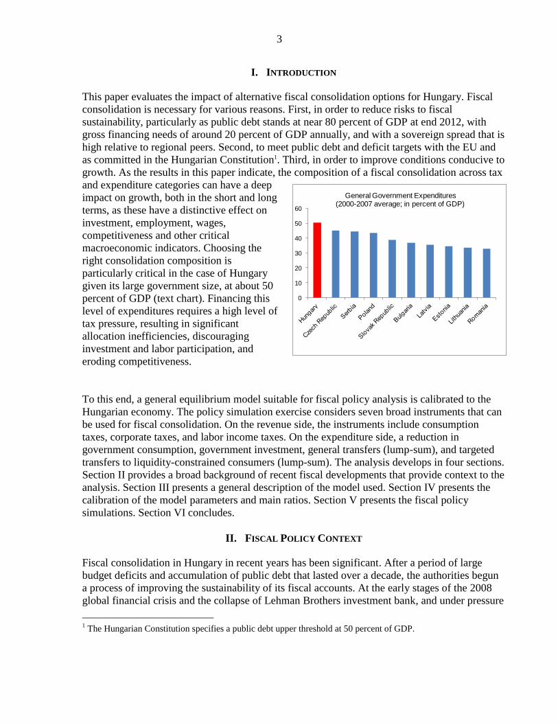
This paper evaluates the impact of alternative fiscal consolidation options for Hungary. Fiscal
consolidation is necessary for various reasons. First, in order to reduce risks to fiscal
sustainability, particularly as public debt stands at near 80 percent of GDP at end 2012, with
gross financing needs of around 20 percent of GDP annually, and with a sovereign spread that is
high relative to regional peers. Second, to meet public debt and deficit targets with the EU and
as committed in the Hungarian Constitution1. Third, in order to improve conditions conducive to
growth. As the results in this paper indicate, the composition of a fiscal consolidation across tax
and expenditure categories can have a deep
impact on growth, both in the short and long
terms, as these have a distinctive effect on
investment, employment, wages,
competitiveness and other critical
macroeconomic indicators. Choosing the
right consolidation composition is
particularly critical in the case of Hungary
given its large government size, at about 50
percent of GDP (text chart). Financing this
level of expenditures requires a high level of
tax pressure, resulting in significant
allocation inefficiencies, discouraging
investment and labor participation, and
eroding competitiveness.
To this end, a general equilibrium model suitable for fiscal policy analysis is calibrated to the
Hungarian economy. The policy simulation exercise considers seven broad instruments that can
be used for fiscal consolidation. On the revenue side, the instruments include consumption
taxes, corporate taxes, and labor income taxes. On the expenditure side, a reduction in
government consumption, government investment, general transfers (lump-sum), and targeted
transfers to liquidity-constrained consumers (lump-sum). The analysis develops in four sections.
Section II provides a broad background of recent fiscal developments that provide context to the
analysis. Section III presents a general description of the model used. Section IV presents the
calibration of the model parameters and main ratios. Section V presents the fiscal policy
simulations. Section VI concludes.
II. FISCAL POLICY CONTEXT
Fiscal consolidation in Hungary in recent years has been significant. After a period of large
budget deficits and accumulation of public debt that lasted over a decade, the authorities begun
a process of improving the sustainability of its fiscal accounts. At the early stages of the 2008
global financial crisis and the collapse of Lehman Brothers investment bank, and under pressure
1 The Hungarian Constitution specifies a public debt upper threshold at 50 percent of GDP.
4
from a reversal in capital flows, currency depreciation, and a collapse in economic growth,
Hungary was the first European nation to enter a Fund-supported program. The program
included a sequence of fiscal consolidation efforts in a broad set of areas, ranging from tax
policy to public employment, pensions, and in several expenditure areas. However, these efforts
were never sufficient to pull Hungary out of the Excessive Deficit Procedure, a commitment
with the EU to reduce fiscal deficits of the general government to below 3 percent of GDP.
Since 2010, there were recurrent efforts and a strong commitment to achieve fiscal
consolidation. The starting point, however, was a reduction in the personal income tax effective
in 2010, to a flat-rate system at 16 percent2, which had an increase in labor participation as main
objective. This initiative came at a significant fiscal cost, and set public finances on an
unsustainable path. To compensate the revenue loss the government introduced sector-specific
levies on bank, energy, and retail sectors, which are largely foreign owned. These levies were
introduced as transitory, and were still insufficient to meet deficit commitments.
The impact of these measures on the fiscal accounts in 2011, however, was masked by the
nationalization of the pension system, which allowed one-off revenues of 9½ percent of GDP.
In that year the government launched the Szell-Kalman Plan, a reform program that focused on
fiscal consolidation and structural reform. It included some ambitious fiscal reforms to be
implemented during 2012 and 2013, of which around ¾ were expenditure-based. The reforms
spread across a broad set of areas including on health, education, social transfers, pensions,
local administrations, and transport. During 2011-2012, there were savings in the expenditure
areas of goods and services, public wages, and transfers to households totaling 2¼ percent of
GDP.
The Convergence Programs of 2011 and 2012 included declining fiscal deficits and public debt
projections. During 2011-2012, however, deteriorating external conditions in the context of the
European crisis slowed revenue performance. In response, the authorities recurrently relied on
largely revenue-based fiscal consolidation packages (two in 2011 and four in 2012). These
packages included an increase in the VAT rate (to become the highest in Europe at 27 percent),
the introduction of multiple small taxes, increase in excises and levies, increase in social
security contributions, and the introduction of simplified business and personal income tax
schemes for small businesses and individuals. In 2013 the budget includes a new tax on
financial transactions, and additional sector-specific taxes on insurance, utilities and telecoms.
In addition the bank levy mentioned above was made permanent. On the expenditure side, the
additional policies since 2011 included across-the-board expenditure restraint by way of
cancelation of budgetary reserves and wage freezes.
III. MODEL OVERVIEW
The results are based on a three-region GIMF (Global Integrated Monetary and Fiscal) general
equilibrium model developed in Kumhof, Laxton, Muir, and Mursula (2010) (KLMM). The
2 Effectively, the Hungarian personal income tax is a two-rate system given that income is taxed in gross terms
(including social security contributions) above a certain threshold.
5
three regions modeled are Hungary (HN), euro area (EU), and Rest of the World (RW). Below
is descriptive presentation of GIMF key features and sectors. More details on the specific
equations and a formal presentation can be found in KLMM.
A. Key Model Features
This section highlights some key model features that are useful to interpret the results.
Non-Ricardian features. The model includes several non-Ricardian features that make revenue
and expenditure fiscal measures non-neutral, both in the short and long terms. In order of
quantitative importance, these features include (i) overlapping generations (OLG) agents with
finite lifetimes and therefore with high subjective discount rates; (ii) life-cycle income profiles
that make wealth less dependent on future labor income; (iii) liquidity-constrained agents; and
(iv) distortionary taxes on labor income, capital income, consumption, and imports.
Nominal and real rigidities. GIMF includes multiple nominal and real rigidities in labor
markets and also in intermediate and final goods markets that result in a cascade of price
rigidities as goods are traded along the production chain from primary producers to final
retailers. Real rigidities include habit persistence in consumption; quantity adjustment costs in
the retail sector; investment adjustment costs and variable capital utilization; and imports’
adjustment costs and productivity spillovers. Nominal rigidities are included as price adjustment
costs by firms, and nominal wage rigidities.
Growth. Steady-state growth is exogenous with the world economy growing at a constant rate.
Population also grows at a constant rate.
Asset markets. Asset markets are assumed to be incomplete. There is complete home bias in
government debt, so that all debt is held by domestic investors in the form of nominal, one-
period bonds denominated in domestic currency. The only internationally traded assets are
nominal one-period bonds denominated in foreign currency. Firms are also owned domestically,
and households receive lump-sum dividend payments from their shareholding in domestic
firms. The commodity sector is owned by both domestic and foreign households.
Risk premium. Risk premium takes the form of a foreign exchange risk premium and a
sovereign risk premium. The foreign exchange risk premium is a non-linear function of current
account to GDP ratio, so that the risk premium becomes higher––and at an increasing rate––as
the current account deficit becomes bigger. The sovereign risk premium is set to be
exogenously, and therefore it is independent from fundamentals.
Monetary policy. The monetary authority responds to economic developments and seeks to
achieve an inflation target. The policy interest rate responds to inflation (concurrent and one-
period-ahead forecast), the size of the inflation gap, and to lagged interest rates.
B. Economy Sectors
In broad terms, the GIMF structure includes the following framework, replicated for all three
regions:
6
Households. There are two types of households: overlapping generations’ (OLG) households
with finite planning horizons (Blanchard, 1985), and liquidity constrained households (LIQ).
Households consume final retailed output and supply labor to unions. Both types of households
are subject to uniform labor income, consumption, and lump-sum taxes. Their income also
derives from financial assets (domestic government and corporate bonds in domestic currency),
international private bonds in foreign currency, and ownership of domestic firms. Households
supply labor to unions. OLG households have several investment options: finance entrepreneurs
through bond purchase; make bank deposits (non-contingent return), and own firm shares that
yield dividends.
Firms. The production structure of the economy includes several stages, which range from
primary producers to retail distributors. Each stage includes a combination of frictions in price
setting and acquisition of inputs that results in a parsimonious response to shocks and also to
changes in economic policy. Primary production is carried by manufacturers producing tradable
and non-tradable goods. For inputs, manufacturers buy capital services from entrepreneurs,
labor from monopolistically competitive unions (who buy labor from households and are
subject to nominal wage rigidities), and raw materials from the world raw-materials market.
Entrepreneurs receive loans from banks (subject to a zero-profit competitive constraint), which
take households’ deposits. Entrepreneurs then purchase capital and rent it to manufacturers, and
decide the rate of capital utilization, which is subject to increasing utilization costs. In addition,
the capital stock is subject to shocks that can result in bankruptcy and undermine entrepreneurs’
loan repayment ability. Banks are subject to monitoring/state verification costs. Manufacturers
are subject to nominal rigidities in price setting, and also to real rigidities in labor hiring and in
the use of raw materials. Capital goods’ producers are subject to investment adjustment costs,
and finance their activities from a combination of domestic and foreign sources. Manufacturers’
domestic sales are purchased by distributors, while foreign sales are purchased by import agents
that are domestically owned but are located in each export destination region (who then sell
their product to foreign distributors).
Distributors. A distribution sector assembles non-tradable goods along with domestic and
foreign tradable goods with imported inputs, with changes in the latter being subject to
adjustment costs. This private sector output is then combined with a publicly-owned capital
stock (infrastructure) and foreign output in order to produce domestic final output which is sold
to consumption goods’ producers, investment goods producers, and to final goods import agents
located at foreign country. Distributors are subject to nominal rigidities (sticky price setting).
Consumption goods output is sold to retailers and the government; investment goods output is
sold to domestic capital goods producers and the government.
Retailers. A monopolistically competitive retail sector sells the goods to consumers at flexible
prices, but with adjustment costs associated with changes in sale volumes. This feature
contributes to generate inertial consumption dynamics, allowing a smoother path of
consumption consistent with time series data. Retailers combine final consumption good
composite from consumption goods producers and raw materials from raw materials producers.
They are subject to adjustment costs to changes in raw material inputs. Their price setting is
subject to real rigidity by way of costly adjustments of sale volume to changes in demand.
7
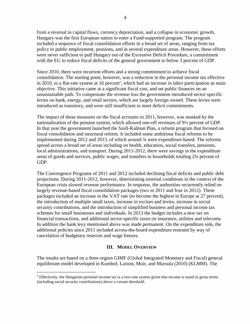
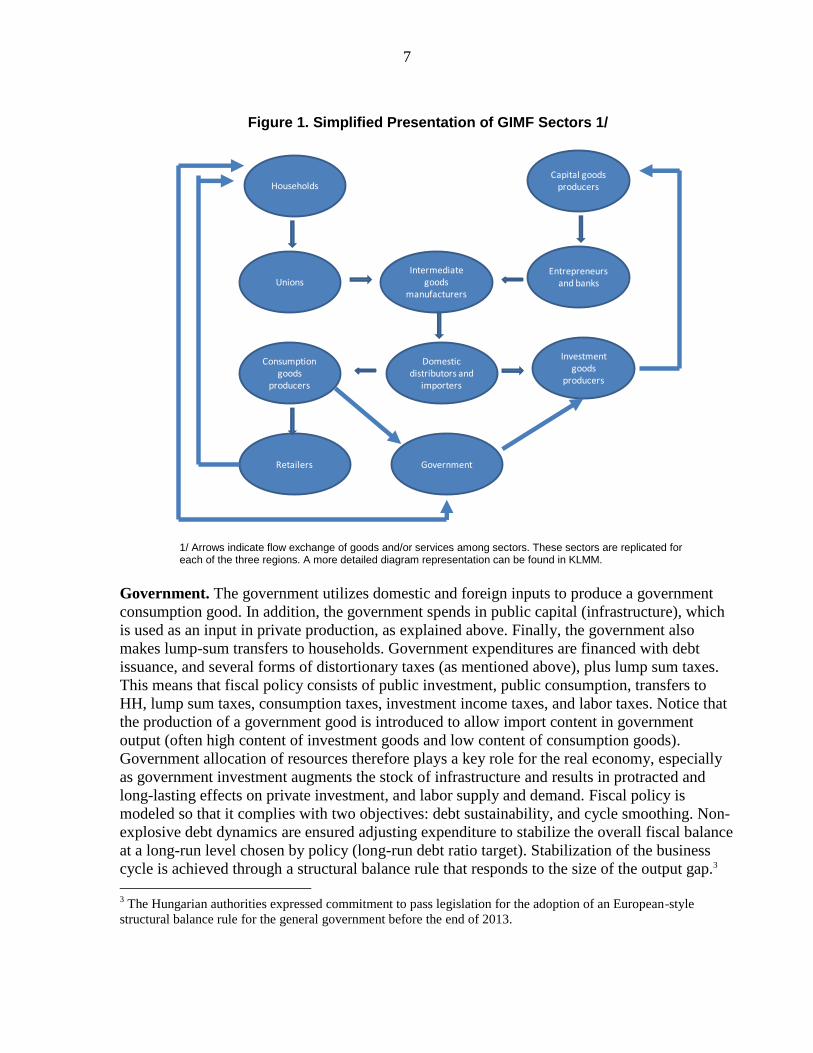
Figure 1. Simplified Presentation of GIMF Sectors 1/
1/ Arrows indicate flow exchange of goods and/or services among sectors. These sectors are replicated for each of the three regions. A more detailed diagram representation can be found in KLMM.
Government. The government utilizes domestic and foreign inputs to produce a government
consumption good. In addition, the government spends in public capital (infrastructure), which
is used as an input in private production, as explained above. Finally, the government also
makes lump-sum transfers to households. Government expenditures are financed with debt
issuance, and several forms of distortionary taxes (as mentioned above), plus lump sum taxes.
This means that fiscal policy consists of public investment, public consumption, transfers to
HH, lump sum taxes, consumption taxes, investment income taxes, and labor taxes. Notice that
the production of a government good is introduced to allow import content in government
output (often high content of investment goods and low content of consumption goods).
Government allocation of resources therefore plays a key role for the real economy, especially
as government investment augments the stock of infrastructure and results in protracted and
long-lasting effects on private investment, and labor supply and demand. Fiscal policy is
modeled so that it complies with two objectives: debt sustainability, and cycle smoothing. Non-
explosive debt dynamics are ensured adjusting expenditure to stabilize the overall fiscal balance
at a long-run level chosen by policy (long-run debt ratio target). Stabilization of the business
cycle is achieved through a structural balance rule that responds to the size of the output gap.3
3 The Hungarian authorities expressed commitment to pass legislation for the adoption of an European-style
structural balance rule for the general government before the end of 2013.
HouseholdsCapital goods
producers
UnionsEntrepreneurs
and banks
Intermediate goods
manufacturers
Domestic distributors and
importers
Investment goods
producers
Retailers Government
Consumption goods
producers
8
IV. CALIBRATION
This section calibrates the GIMF model to key features of the Hungarian economy. When there
are no specific estimates for Hungary, main structural parameters are kept the same as KLLM,
in line with the literature. Other parameters are derived from national accounts, ComTrade, and
GFS databases. Table 1 lists the main long-run assumptions, which correspond to the steady
state. It represents the baseline projection against which the policy simulations are compared in
the following sections.
Hungary represents 0.15 percent of world population and 0.25 percent of world GDP (PPP
adjusted). The steady-state world technology growth rate is set at 1.5 percent per year, and the
world population rate is set to grow at 1 percent. Inflation was set at 2 percent in Hungary and
the euro area (EU), and at 2.5 percent in the rest of the world (RW). The world real interest rate
is equalized across countries at 3 percent per annum4. The external financing premium function
is calibrated to produce 250 basis points premium over international interest rates at steady state
net foreign liabilities to GDP ratio of 0. Factor shares in aggregate production are set at
40 percent for capital and 60 percent for labor for the three regions. The calibrated shares of
labor for the Hungarian tradable sector is 54 percent, and for the non-tradable sector is 71
percent, which are higher than in the other two regions.
The liquidity constrained agents are assumed to represent 30 percent of consumers in Hungary,
30 percent in the euro area and 40 percent in the rest of the world. The share of these agents in
dividend income is assumed to be half of their share in the population. The real and price
adjustments costs are calibrated to yield plausible dynamics over the first couple of years
following the shock. The calibrations of the parameters affecting preferences, economic sectors,
and other structural parameters are presented in Appendix I.
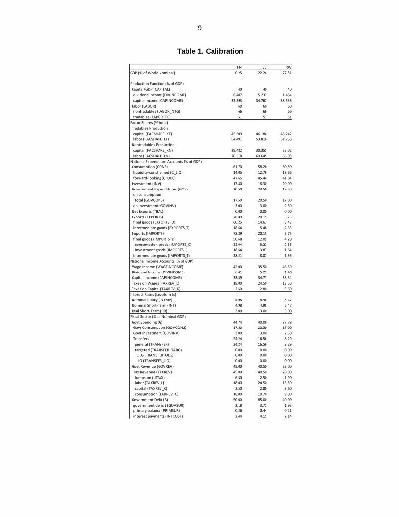
Table 1 also shows the decomposition of steady-state GDP at producer prices into its
expenditure components. Investment shares are set at 17.8 percent for Hungary, 18.3 percent for
the euro area and 20 percent for the rest of the world. The rest of the expenditure shares are
obtained endogenously from the evolution of the economy, including as a result of preference
and technology parameters. The resulting values are in line with the historical data.
The bottom section of Table 1 shows the calibrations for the government revenue and
expenditure shares in percent of GDP. Revenues are set at 45 percent of GDP (general
government), in line with recent historical trends. The long-term debt target is set at 50 percent,
which is the upper threshold set in the Hungarian Constitution. This long-term steady state debt
stock, together with equilibrium interest rates and long-term growth, result in a primary surplus
of ¼ percent of GDP in steady-state. Government consumption is calibrated at 17.5 percent of
GDP for Hungary, which is about the value of the sum of general government expenditure in
goods and services and wages and salaries. Investment is calibrated at 3 percent of GDP, also
4 The subjective (or “pure”) discount factors are calculated consistent with these values.
9
Table 1. Calibration
HN EU RW
GDP (% of World Nominal) 0.25 22.24 77.51
Production Function (% of GDP)
Capital/GDP (CAPITAL) 40 40 40
dividend income (DIVINCOME) 6.407 5.233 1.464
capital income (CAPINCOME) 33.593 34.767 38.536
Labor (LABOR) 60 60 60
nontradables (LABOR_NTG) 66 66 66
tradables (LABOR_TG) 51 51 51
Factor Shares (% total)
Tradables Production
capital (FACSHARE_KT) 45.509 46.184 48.242
labor (FACSHARE_LT) 54.491 53.816 51.758
Nontradables Production
capital (FACSHARE_KN) 29.482 30.355 33.02
labor (FACSHARE_LN) 70.518 69.645 66.98
National Expenditure Accounts (% of GDP)
Consumption (CONS) 61.70 58.20 60.50
liquidity-constrained (C_LIQ) 14.05 12.76 18.66
forward-looking (C_OLG) 47.65 45.44 41.84
Investment (INV) 17.80 18.30 20.00
Government Expenditures (GOV) 20.50 23.50 19.50
on consumption
total (GOVCONS) 17.50 20.50 17.00
on investment (GOVINV) 3.00 3.00 2.50
Net Exports (TBAL) 0.00 0.00 0.00
Exports (EXPORTS) 78.89 20.15 5.75
final goods (EXPORTS_D) 60.25 14.67 3.43
intermediate goods (EXPORTS_T) 18.64 5.48 2.33
Imports (IMPORTS) 78.89 20.15 5.75
final goods (IMPORTS_D) 50.68 12.09 4.20
consumption goods (IMPORTS_C) 32.04 8.22 2.55
investment goods (IMPORTS_I) 18.64 3.87 1.64
intermediate goods (IMPORTS_T) 28.21 8.07 1.55
National Income Accounts (% of GDP)
Wage Income (WAGEINCOME) 42.00 35.50 46.50
Dividend Income (DIVINCOME) 6.41 5.23 1.46
Capital Income (CAPINCOME) 33.59 34.77 38.54
Taxes on Wages (TAXREV_L) 18.00 24.50 13.50
Taxes on Capital (TAXREV_K) 2.50 2.80 3.60
Interest Rates (Levels in %)
Nominal Policy (INTMP) 4.98 4.98 5.47
Nominal Short-Term (INT) 4.98 4.98 5.47
Real Short-Term (RR) 3.00 3.00 3.00
Fiscal Sector (% of Nominal GDP)
Govt Spending (G) 44.74 40.06 27.79
Govt Consumption (GOVCONS) 17.50 20.50 17.00
Govt Investment (GOVINV) 3.00 3.00 2.50
Transfers 24.24 16.56 8.29
general (TRANSFER) 24.24 16.56 8.29
targeted (TRANSFER_TARG) 0.00 0.00 0.00
OLG (TRANSFER_OLG) 0.00 0.00 0.00
LIQ (TRANSFER_LIQ) 0.00 0.00 0.00
Govt Revenue (GOVREV) 45.00 40.50 28.00
Tax Revenue (TAXREV) 45.00 40.50 28.00
lumpsum (LSTAX) 6.50 2.50 1.90
labor (TAXREV_L) 18.00 24.50 13.50
capital (TAXREV_K) 2.50 2.80 3.60
consumption (TAXREV_C) 18.00 10.70 9.00
Government Debt (B) 50.00 85.00 40.00
government deficit (GOVSUR) 2.18 3.71 1.93
primary balance (PRIMSUR) 0.26 0.44 0.21
interest payments (INTCOST) 2.44 4.15 2.14
10
consistent with historical trends5. The calibrations for EU and RW are also displayed in the
second and third columns of Table 1.
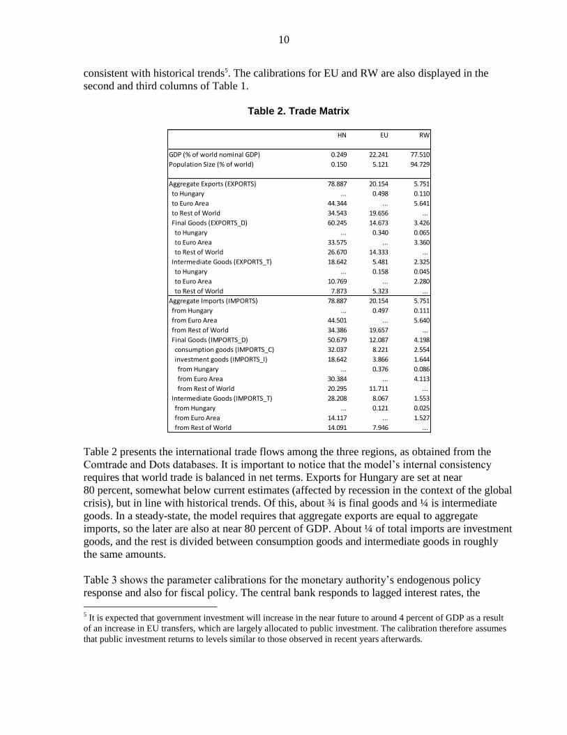
Table 2. Trade Matrix
Table 2 presents the international trade flows among the three regions, as obtained from the
Comtrade and Dots databases. It is important to notice that the model’s internal consistency
requires that world trade is balanced in net terms. Exports for Hungary are set at near
80 percent, somewhat below current estimates (affected by recession in the context of the global
crisis), but in line with historical trends. Of this, about ¾ is final goods and ¼ is intermediate
goods. In a steady-state, the model requires that aggregate exports are equal to aggregate
imports, so the later are also at near 80 percent of GDP. About ¼ of total imports are investment
goods, and the rest is divided between consumption goods and intermediate goods in roughly
the same amounts.
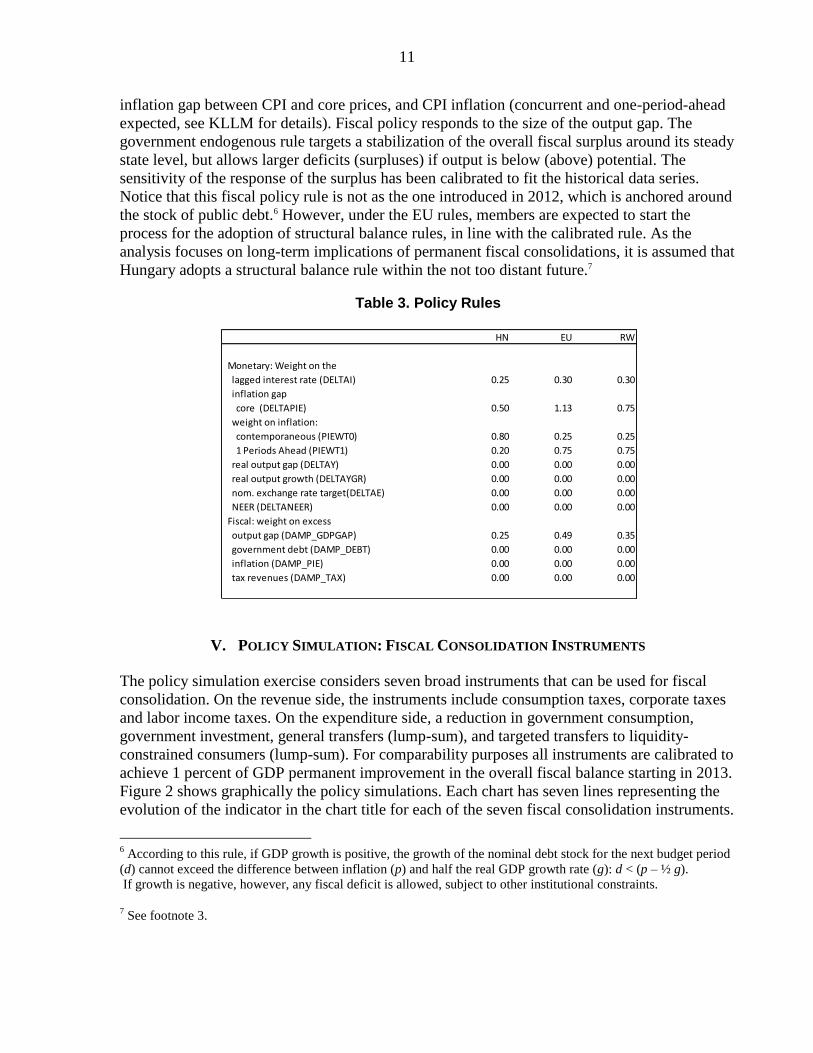
Table 3 shows the parameter calibrations for the monetary authority’s endogenous policy
response and also for fiscal policy. The central bank responds to lagged interest rates, the
5 It is expected that government investment will increase in the near future to around 4 percent of GDP as a result
of an increase in EU transfers, which are largely allocated to public investment. The calibration therefore assumes
that public investment returns to levels similar to those observed in recent years afterwards.
HN EU RW
GDP (% of world nominal GDP) 0.249 22.241 77.510
Population Size (% of world) 0.150 5.121 94.729
Aggregate Exports (EXPORTS) 78.887 20.154 5.751
to Hungary ... 0.498 0.110
to Euro Area 44.344 ... 5.641
to Rest of World 34.543 19.656 ...
Final Goods (EXPORTS_D) 60.245 14.673 3.426
to Hungary ... 0.340 0.065
to Euro Area 33.575 ... 3.360
to Rest of World 26.670 14.333 ...
Intermediate Goods (EXPORTS_T) 18.642 5.481 2.325
to Hungary ... 0.158 0.045
to Euro Area 10.769 ... 2.280
to Rest of World 7.873 5.323 ...
Aggregate Imports (IMPORTS) 78.887 20.154 5.751
from Hungary ... 0.497 0.111
from Euro Area 44.501 ... 5.640
from Rest of World 34.386 19.657 ...
Final Goods (IMPORTS_D) 50.679 12.087 4.198
consumption goods (IMPORTS_C) 32.037 8.221 2.554
investment goods (IMPORTS_I) 18.642 3.866 1.644
from Hungary ... 0.376 0.086
from Euro Area 30.384 ... 4.113
from Rest of World 20.295 11.711 ...
Intermediate Goods (IMPORTS_T) 28.208 8.067 1.553
from Hungary ... 0.121 0.025
from Euro Area 14.117 ... 1.527
from Rest of World 14.091 7.946 ...
11
inflation gap between CPI and core prices, and CPI inflation (concurrent and one-period-ahead
expected, see KLLM for details). Fiscal policy responds to the size of the output gap. The
government endogenous rule targets a stabilization of the overall fiscal surplus around its steady
state level, but allows larger deficits (surpluses) if output is below (above) potential. The
sensitivity of the response of the surplus has been calibrated to fit the historical data series.
Notice that this fiscal policy rule is not as the one introduced in 2012, which is anchored around
the stock of public debt.6 However, under the EU rules, members are expected to start the
process for the adoption of structural balance rules, in line with the calibrated rule. As the
analysis focuses on long-term implications of permanent fiscal consolidations, it is assumed that
Hungary adopts a structural balance rule within the not too distant future.7
Table 3. Policy Rules
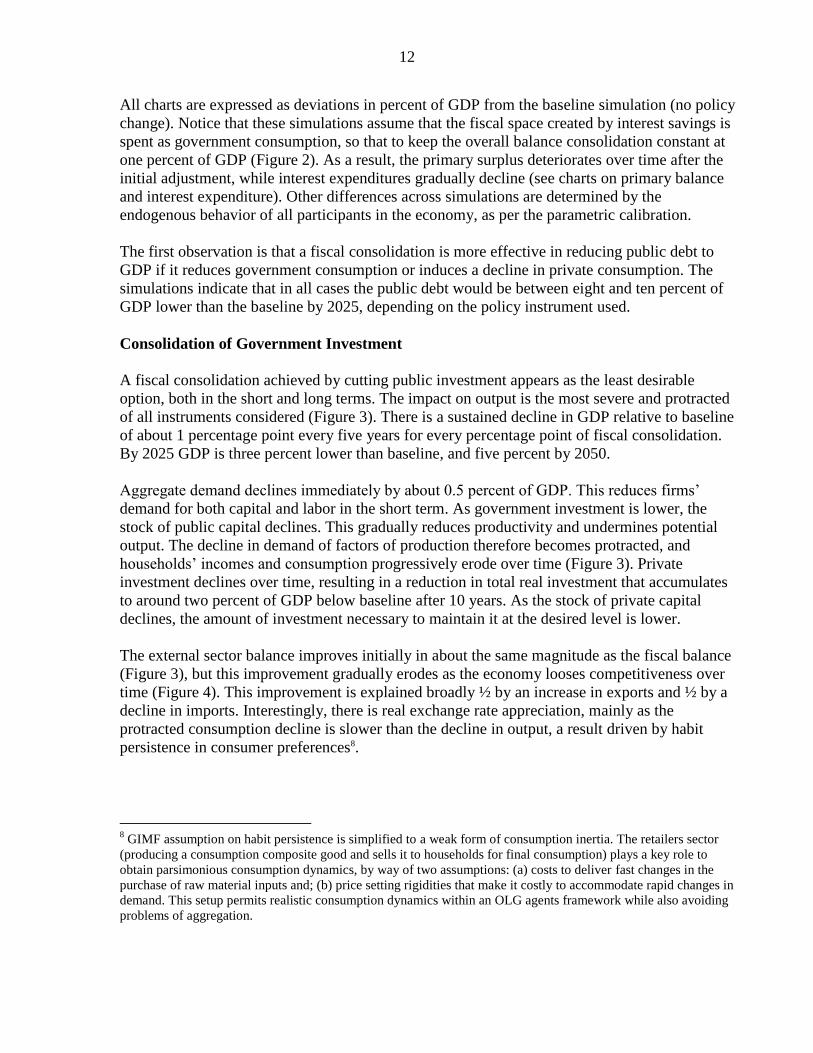
V. POLICY SIMULATION: FISCAL CONSOLIDATION INSTRUMENTS
The policy simulation exercise considers seven broad instruments that can be used for fiscal
consolidation. On the revenue side, the instruments include consumption taxes, corporate taxes
and labor income taxes. On the expenditure side, a reduction in government consumption,
government investment, general transfers (lump-sum), and targeted transfers to liquidity-
constrained consumers (lump-sum). For comparability purposes all instruments are calibrated to
achieve 1 percent of GDP permanent improvement in the overall fiscal balance starting in 2013.
Figure 2 shows graphically the policy simulations. Each chart has seven lines representing the
evolution of the indicator in the chart title for each of the seven fiscal consolidation instruments.
6 According to this rule, if GDP growth is positive, the growth of the nominal debt stock for the next budget period
(d) cannot exceed the difference between inflation (p) and half the real GDP growth rate (g): d < (p – ½ g).
If growth is negative, however, any fiscal deficit is allowed, subject to other institutional constraints.
7 See footnote 3.
HN EU RW
Monetary: Weight on the
lagged interest rate (DELTAI) 0.25 0.30 0.30
inflation gap
core (DELTAPIE) 0.50 1.13 0.75
weight on inflation:
contemporaneous (PIEWT0) 0.80 0.25 0.25
1 Periods Ahead (PIEWT1) 0.20 0.75 0.75
real output gap (DELTAY) 0.00 0.00 0.00
real output growth (DELTAYGR) 0.00 0.00 0.00
nom. exchange rate target(DELTAE) 0.00 0.00 0.00
NEER (DELTANEER) 0.00 0.00 0.00
Fiscal: weight on excess
output gap (DAMP_GDPGAP) 0.25 0.49 0.35
government debt (DAMP_DEBT) 0.00 0.00 0.00
inflation (DAMP_PIE) 0.00 0.00 0.00
tax revenues (DAMP_TAX) 0.00 0.00 0.00
12
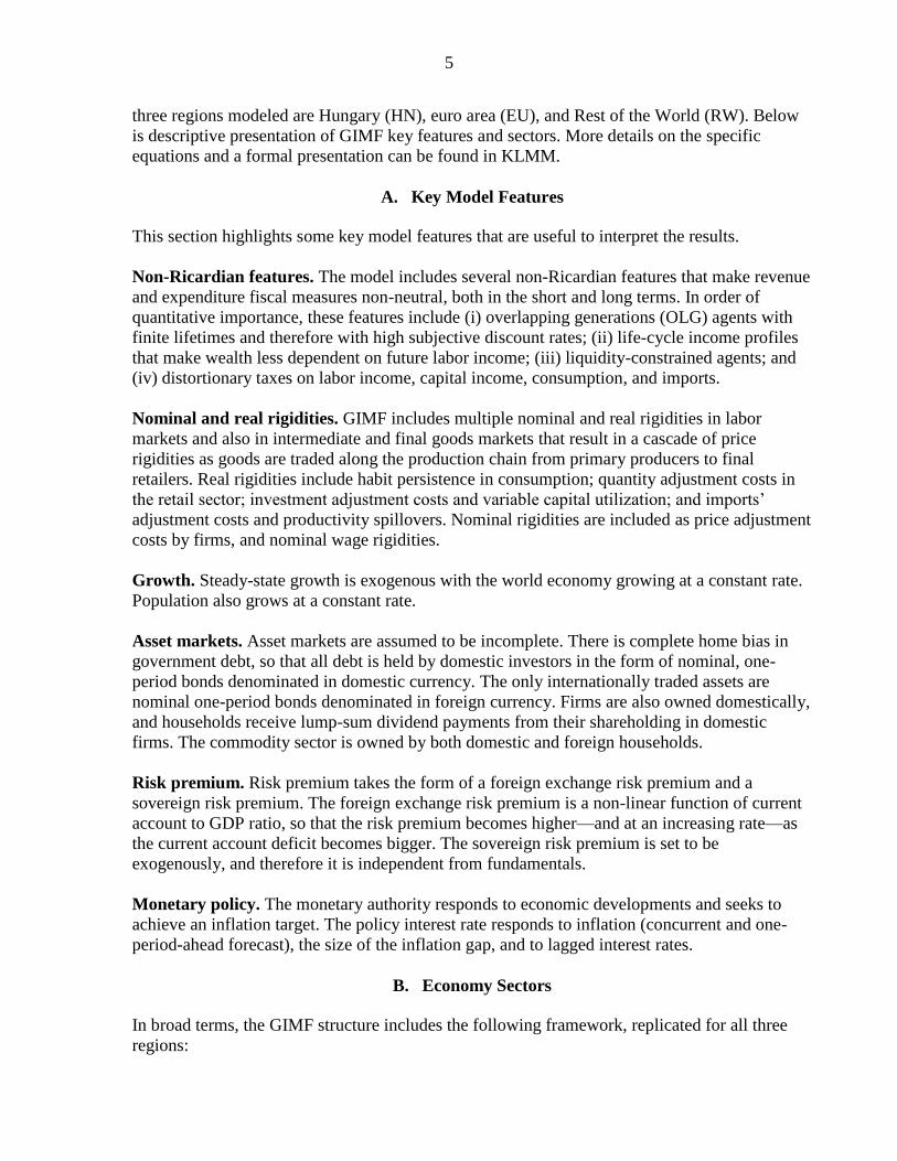
All charts are expressed as deviations in percent of GDP from the baseline simulation (no policy
change). Notice that these simulations assume that the fiscal space created by interest savings is
spent as government consumption, so that to keep the overall balance consolidation constant at
one percent of GDP (Figure 2). As a result, the primary surplus deteriorates over time after the
initial adjustment, while interest expenditures gradually decline (see charts on primary balance
and interest expenditure). Other differences across simulations are determined by the
endogenous behavior of all participants in the economy, as per the parametric calibration.
The first observation is that a fiscal consolidation is more effective in reducing public debt to
GDP if it reduces government consumption or induces a decline in private consumption. The
simulations indicate that in all cases the public debt would be between eight and ten percent of
GDP lower than the baseline by 2025, depending on the policy instrument used.
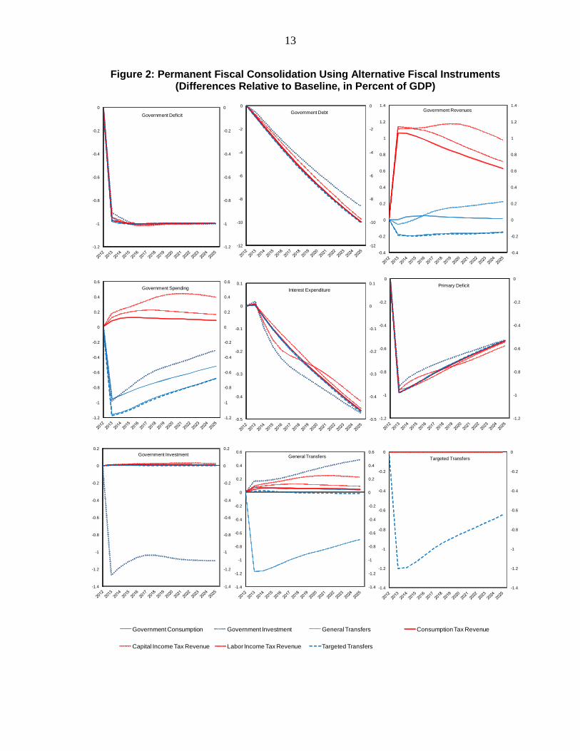
Consolidation of Government Investment
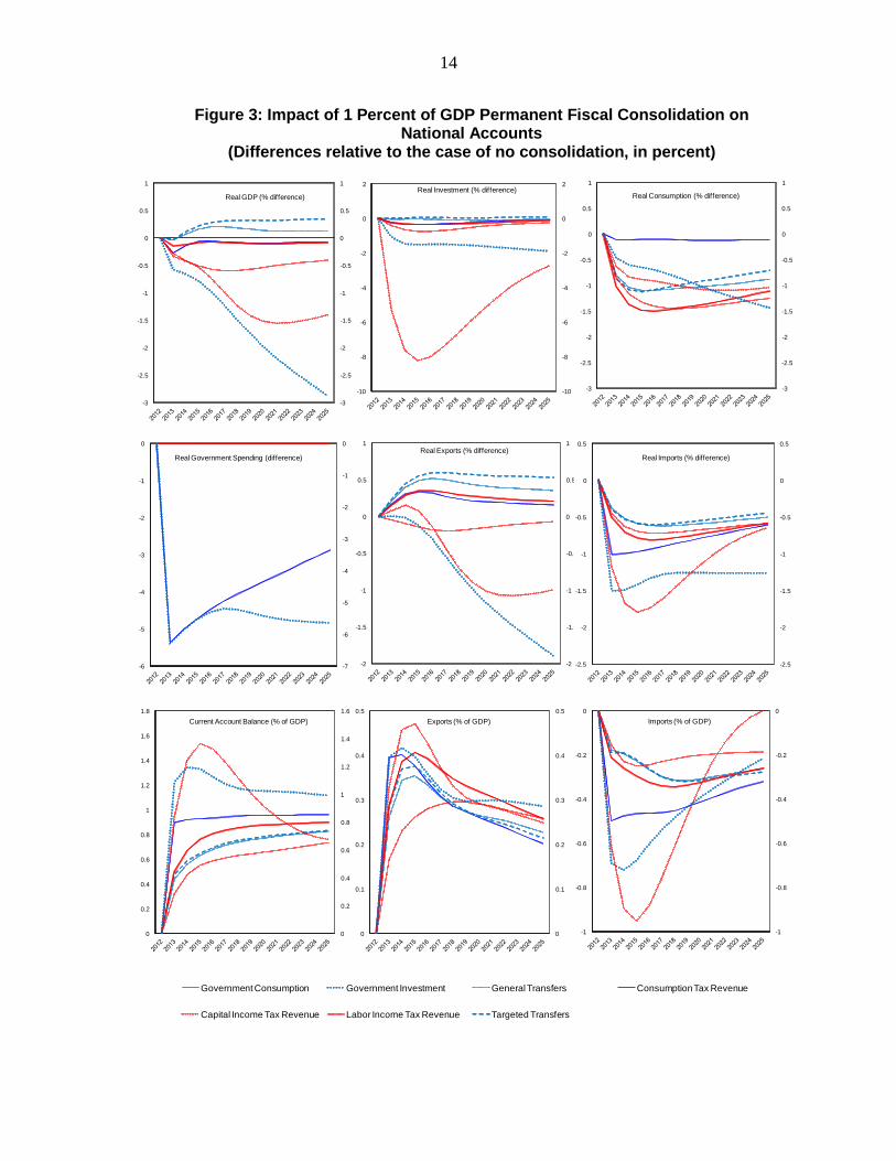
A fiscal consolidation achieved by cutting public investment appears as the least desirable
option, both in the short and long terms. The impact on output is the most severe and protracted
of all instruments considered (Figure 3). There is a sustained decline in GDP relative to baseline
of about 1 percentage point every five years for every percentage point of fiscal consolidation.
By 2025 GDP is three percent lower than baseline, and five percent by 2050.
Aggregate demand declines immediately by about 0.5 percent of GDP. This reduces firms’
demand for both capital and labor in the short term. As government investment is lower, the
stock of public capital declines. This gradually reduces productivity and undermines potential
output. The decline in demand of factors of production therefore becomes protracted, and
households’ incomes and consumption progressively erode over time (Figure 3). Private
investment declines over time, resulting in a reduction in total real investment that accumulates
to around two percent of GDP below baseline after 10 years. As the stock of private capital
declines, the amount of investment necessary to maintain it at the desired level is lower.
The external sector balance improves initially in about the same magnitude as the fiscal balance
(Figure 3), but this improvement gradually erodes as the economy looses competitiveness over
time (Figure 4). This improvement is explained broadly ½ by an increase in exports and ½ by a
decline in imports. Interestingly, there is real exchange rate appreciation, mainly as the
protracted consumption decline is slower than the decline in output, a result driven by habit
persistence in consumer preferences8.
8 GIMF assumption on habit persistence is simplified to a weak form of consumption inertia. The retailers sector
(producing a consumption composite good and sells it to households for final consumption) plays a key role to
obtain parsimonious consumption dynamics, by way of two assumptions: (a) costs to deliver fast changes in the
purchase of raw material inputs and; (b) price setting rigidities that make it costly to accommodate rapid changes in
demand. This setup permits realistic consumption dynamics within an OLG agents framework while also avoiding
problems of aggregation.
13
Figure 2: Permanent Fiscal Consolidation Using Alternative Fiscal Instruments (Differences Relative to Baseline, in Percent of GDP)
-12
-10
-8
-6
-4
-2
0
-12
-10
-8
-6
-4
-2
0
Government Debt
-1.2
-1
-0.8
-0.6
-0.4
-0.2
0
-1.2
-1
-0.8
-0.6
-0.4
-0.2
0
Government Deficit
-0.5
-0.4
-0.3
-0.2
-0.1
0
0.1
-0.5
-0.4
-0.3
-0.2
-0.1
0
0.1
Interest Expenditure
-1.2
-1
-0.8
-0.6
-0.4
-0.2
0
0.2
0.4
0.6
-1.2
-1
-0.8
-0.6
-0.4
-0.2
0
0.2
0.4
0.6
Government Spending
-1.2
-1
-0.8
-0.6
-0.4
-0.2
0
-1.2
-1
-0.8
-0.6
-0.4
-0.2
0
Primary Deficit
-0.4
-0.2
0
0.2
0.4
0.6
0.8
1
1.2
1.4
-0.4
-0.2
0
0.2
0.4
0.6
0.8
1
1.2
1.4
Government Revenues
-1.4
-1.2
-1
-0.8
-0.6
-0.4
-0.2
0
0.2
-1.4
-1.2
-1
-0.8
-0.6
-0.4
-0.2
0
0.2
Government Investment
-1.4
-1.2
-1
-0.8
-0.6
-0.4
-0.2
0
0.2
0.4
0.6
-1.4
-1.2
-1
-0.8
-0.6
-0.4
-0.2
0
0.2
0.4
0.6General Transfers
-1.4
-1.2
-1
-0.8
-0.6
-0.4
-0.2
0
-1.4
-1.2
-1
-0.8
-0.6
-0.4
-0.2
0
Targeted Transfers
Government Consumption Government Investment General Transfers Consumption Tax Revenue
Capital Income Tax Revenue Labor Income Tax Revenue Targeted Transfers
14
Figure 3: Impact of 1 Percent of GDP Permanent Fiscal Consolidation on National Accounts
(Differences relative to the case of no consolidation, in percent)
-3
-2.5
-2
-1.5
-1
-0.5
0
0.5
1
-3
-2.5
-2
-1.5
-1
-0.5
0
0.5
1
Real GDP (% difference)
-10
-8
-6
-4
-2
0
2
-10
-8
-6
-4
-2
0
2Real Investment (% difference)
-3
-2.5
-2
-1.5
-1
-0.5
0
0.5
1
-3
-2.5
-2
-1.5
-1
-0.5
0
0.5
1
Real Consumption (% difference)
-7
-6
-5
-4
-3
-2
-1
0
-6
-5
-4
-3
-2
-1
0
Real Government Spending (difference)
-2
-1.5
-1
-0.5
0
0.5
1
-2
-1.5
-1
-0.5
0
0.5
1
Real Exports (% difference)
-2.5
-2
-1.5
-1
-0.5
0
0.5
-2.5
-2
-1.5
-1
-0.5
0
0.5
Real Imports (% difference)
Government Consumption Government Investment General Transfers Consumption Tax Revenue
Capital Income Tax Revenue Labor Income Tax Revenue Targeted Transfers
0
0.2
0.4
0.6
0.8
1
1.2
1.4
1.6
0
0.2
0.4
0.6
0.8
1
1.2
1.4
1.6
1.8
Current Account Balance (% of GDP)
0
0.1
0.2
0.3
0.4
0.5
0
0.1
0.2
0.3
0.4
0.5
Exports (% of GDP)
-1
-0.8
-0.6
-0.4
-0.2
0
-1
-0.8
-0.6
-0.4
-0.2
0
Imports (% of GDP)

15
Figure 4: Impact of 1 Percent of GDP Permanent Fiscal Consolidation on Inflation, Exchange Rates and Interest Rates
(Differences Relative to the Case of No Consolidation, in Percent)
-1
-0.8
-0.6
-0.4
-0.2
0
0.2
0.4
-1
-0.8
-0.6
-0.4
-0.2
0
0.2
0.4
Real Effective Exchange Rate (+ is depreciation)
-0.12
-0.1
-0.08
-0.06
-0.04
-0.02
0
0.02
0.04
-0.12
-0.1
-0.08
-0.06
-0.04
-0.02
0
0.02
0.04
Real Interest Rate (percentage pts.)
-0.1
-0.08
-0.06
-0.04
-0.02
0
0.02
-0.1
-0.08
-0.06
-0.04
-0.02
0
0.02Real Long-term Interest Rate (percentage pts.)
-2
-1.5
-1
-0.5
0
0.5
1
-2
-1.5
-1
-0.5
0
0.5
1Real Wage (producer cost, percentage pts.)
Government Consumption Government Investment General Transfers Consumption Tax Revenue
Capital Income Tax Revenue Labor Income Tax Revenue Targeted Transfers
-0.2
-0.18
-0.16
-0.14
-0.12
-0.1
-0.08
-0.06
-0.04
-0.02
0
0.02
0.04
-0.2
-0.18
-0.16
-0.14
-0.12
-0.1
-0.08
-0.06
-0.04
-0.02
0
0.02
0.04
Consumer Price Inflation (percentage points)
-0.2
-0.18
-0.16
-0.14
-0.12
-0.1
-0.08
-0.06
-0.04
-0.02
0
0.02
0.04
-0.2
-0.18
-0.16
-0.14
-0.12
-0.1
-0.08
-0.06
-0.04
-0.02
0
0.02
0.04
Core Inflation (percentage points)
-3
-2.5
-2
-1.5
-1
-0.5
0
0.5
-3
-2.5
-2
-1.5
-1
-0.5
0
0.5
Nominal Effective Exchange Rate (+ is depreciation)
-0.3
-0.25
-0.2
-0.15
-0.1
-0.05
0
0.05
0.1
-0.3
-0.25
-0.2
-0.15
-0.1
-0.05
0
0.05
0.1
Short Term Nominal Interest Rate (percentage pts.)
-0.3
-0.25
-0.2
-0.15
-0.1
-0.05
0
0.05
0.1
-0.3
-0.25
-0.2
-0.15
-0.1
-0.05
0
0.05
0.1
Nominal Policy Rate (percentage pts.)
16
Consistent with these developments, there is a decline in inflation and interest rates that is
largest in magnitude compared to other forms of consolidation (Figure 4). Consumer and core
inflation decline 0.1 percentage points below baseline in the short term, with this decline
picking by year three at near 0.2 percentage points. The net effect is also a decline in real
interest rates, as de-investment across sectors materializes. The decline in real wages is the most
significant when comparing across all consolidation instruments considered, at 1 percent after
five years, and more than 3 percent in the long–term (beyond the time horizon span shown in
the chart in Figure 4).
Consolidation of Government Consumption
If fiscal consolidation is achieved with a reduction of government consumption in goods and
services and/or wage expenditures, aggregate demand declines in the short-term about ¼
percent below baseline (Figure 3). Afterwards it recovers, but only partially, remaining short of
the baseline level. Notice that this result would in general be different to the predicted fiscal
multiplier of a fiscal stimulus, which is a transitory policy by definition. In sharp contrast with a
cut in public investment, private investment remains almost unaffected, and private
consumption increases to almost fully offset the decline in public consumption. The current
account balance improves proportionally, with roughly a ½ split between an improvement in
exports and a decline in imports. This mild economic response is largely explained by the high
degree of openness of the Hungarian economy. The demand impact from public consumption
retrenchment has a large impact on the demand of imports, rather than on domestic goods.
Inflation decline is minimal, and the nominal and real exchange rate show a small amount of
depreciation that peaks in the first year at 0.2 percent compared to baseline (for both core and
CPI). Real wages decline by less than 0.5 percent in the short–term, and partially recover over
the long-term
Consolidation of Government Transfers—General and Targeted
The initial impact of a cut in transfers on output is mute (Figure 3). Consumption declines
immediately and in the same amount as the transfers’ cut. Moreover, output increases in the
medium and long term relative to baseline, and more so in the case of a cut in targeted transfers
(0.4 percent of GDP relative to baseline) than in the case of general transfers (0.1 percent). The
current account balance improves relative to baseline, but less than in the cases of consolidation
via government consumption and investment analyzed above. The current account improves by
0.4 percent of GDP on impact, and continues to improve over time to stabilize at around
0.8 percent of GDP above baseline. This different current account behavior is the result of a
milder decline in imports than in the two cases above.
The muted impact on output in the short term is explained by the endogenous response of the
economy. Unlike in the case of a consolidation cutting public investment, total investment
remains virtually unaffected. As households disposable income is reduced with the cut in
transfers, labor participation increases, boosting output and having an offsetting effect. With
lower overall household income the decline in consumption becomes protracted and results in
permanent currency depreciation in real terms (mainly from a nominal depreciation). Moreover,
17
the currency depreciation reduces the producer-cost of labor, further increasing the demand for
labor and output. All in all, the improvement in external competitiveness allows output to
remain at the same level as in baseline in the short term despite a decline in private consumption
as the external demand offsets the decline in domestic demand.
Over the medium and long terms, the improvement in competitiveness results in higher output
permanently. The increases in labor participation and labor demand explained above is large
and protracted, given the permanent nature of the cut in transfers. In addition, the gradual
reduction in government debt reduces interest rates further, creating fiscal space which in the
simulation is allocated to government consumption and provides further stimulus to aggregate
demand. This allows some reversal of the short-term improvement in external accounts
(Figure 4). In addition, the sustained improvement in the external balance results in private
sector accumulation of net foreign assets, and a gradual increase in the non-wage income of the
OLG (forward-looking non-myopic) consumers. This last effect reduces the negative short-term
impact of the cut in transfers and contributes to the gradual recovery in consumption.
The dynamics analyzed above are more pronounced in the case of a cut in transfers that are
targeted to liquidity-constrained agents, in comparison with the case of a cut in general
transfers. As liquidity-constrained agents do not accumulate assets by assumption, they have
less room to cushion the decline in income with other sources of income and savings, and their
response is more pronounced (also because the same amount of fiscal consolidation is
concentrated in a smaller number of households).
Consolidation with Consumption Taxes
Increasing consumption taxes permanently to achieve an improvement in the overall balance of
1 percent of GDP reduces growth by 0.2 percent in the first year (Figure 3). Afterwards, GDP
growth recovers in a small amount, but never back to baseline levels. Private consumption,
however, declines significantly, more than in any other policy instrument considered. Real
consumption declines 1 percent of GDP in the first year, 1.5 percent by the third year, and
recovers gradually afterwards. The recovery, however, is explained in part by the assumption on
the allocation of the fiscal space created by the reduction in public debt to government
consumption, as explained above.
The external accounts improve, as expected, but, interestingly, less so than under a reduction in
government investment and government consumption (Figure 3). The current account balance
increases gradually to reach 0.8 percent of GDP by year three and stabilizing below 1 percent of
GDP in the long–term. This is determined by an increase in exports that peaks at 0.4 percent of
GDP by year three and a contraction in imports that is somewhat more protracted and peaks also
at near 0.4 percent of GDP. Inflation declines to 0.02 percentage points below baseline over the
first three years, as the impact on prices of a decline in consumption offsets the price level effect
of taxes, but then recovers back to baseline in the long–term (Figure 4). Interest rates also
reflect the lack of demand and move downward, while the nominal exchange rate depreciates by
less than 0.2 percent, and allows a real exchange rate depreciation of about the same amount.
This exchange rate depreciation is very protracted.
18
The results above indicate that there is a contractionary effect, including a decline in growth,
inflation, interest rates, and exchange rate depreciation. This contraction, however, is small
relative to the size of the consolidation. The decline in output is less than ¼ the size of the
improvement in the fiscal surplus targeted, and inflation, interest rate, and exchange rates show
relatively small changes. The reasons behind this result are twofold. First, the increase in
consumption taxes stimulates savings. As a result forward looking (OLG) consumers internalize
an increase in wealth income, which moderates the decline in consumption (aided also by habit
persistence in consumption). The decline in interest rates also increases investment and the
capital stock, moderating the decline in output as time passes. This also explains why real wage
declines, as determined by a lower demand, but less so than under other consolidation options
(0.2 percent below baseline by year three, protracted). Second, with Hungary being a very open
economy, the external balance improves considerably, more than ¾ the size of the
consolidation, as the exchange rate depreciates in real terms. This implies that the switching
effect from domestic to external demand is relatively large, cushioning the domestic demand
impact.
Consolidation with Corporate Income Taxes
A consolidation with taxes on corporations is contractionary in the short–term, and becomes
significantly more so in the medium term, second only to a reduction in government investment.
Output declines 0.4 percentage points below baseline in the first year, then 0.5 percent by
year five, and continues to stimulate a steady decline in output that peaks after ten years, at
1.5 percentage points below baseline (Figure 3). The main driver of this result is a decline in
private investment, which is sustained for a long period of time until the point the capital stock
reaches its desired level. Indeed, investment over 5 percentage points below baseline in year 1,
and more than 8 percentage points by year 3, when it reaches its lowest point. This investment
decline is far more significant than in any other of the policy alternatives considered. It is
interesting to notice that in year 1 private consumption declines to 0.6 percent below baseline,
which is about ½ of the decline that would be obtained under the other two tax alternatives and
also if government transfers were reduced. This indicates that the distributional impact of this
option is, however, not without cost. Notice that real wages also exhibit a significant decline, of
about the same magnitude than the one predicted under a decline in government investment
during the first five years after the policy is implemented. By year five real wages are 1 percent
below baseline, and remain at around that level thereafter (Figure 4).
The external accounts show the biggest improvements in the short term of all policy alternatives
under analysis. The improvement in the current account balance peaks at 1 ½ percent of GDP
by year 3 (Figure 3). Of this, about 1 percent is due to a contraction in imports, which in this
case are augmented by the decline in imports of investment goods, and ½ percent by an increase
in exports.
Inflation decline is of more than 0.1 percent below baseline, consistent with the general decline
in aggregate demand and output. This is not a big amount, but is the second largest decline
when comparing across the consolidation alternatives. The same observation applies to nominal
and real interest rates. As with the case of a cut in government investment, the real exchange
rate appreciates, a result that appears unintuitive given that the decline in output and demand is
19
second to largest. The underlying reasons are the same as in the case of government investment
consolidation.
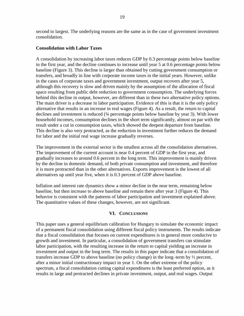
Consolidation with Labor Taxes
A consolidation by increasing labor taxes reduces GDP by 0.3 percentage points below baseline
in the first year, and the decline continues to increase until year 5 at 0.6 percentage points below
baseline (Figure 3). This decline is larger than obtained by cutting government consumption or
transfers, and broadly in line with corporate income taxes in the initial years. However, unlike
in the cases of corporate taxes and government investment, output recovers after year 5,
although this recovery is slow and driven mainly by the assumption of the allocation of fiscal
space resulting from public debt reduction to government consumption. The underlying forces
behind this decline in output, however, are different than in these two alternative policy options.
The main driver is a decrease in labor participation. Evidence of this is that it is the only policy
alternative that results in an increase in real wages (Figure 4). As a result, the return to capital
declines and investment is reduced (¾ percentage points below baseline by year 3). With lower
household incomes, consumption declines in the short term significantly, almost on par with the
result under a cut in consumption taxes, which showed the deepest departure from baseline.
This decline is also very protracted, as the reduction in investment further reduces the demand
for labor and the initial real wage increase gradually reverses.
The improvement in the external sector is the smallest across all the consolidation alternatives.
The improvement of the current account is near 0.4 percent of GDP in the first year, and
gradually increases to around 0.6 percent in the long term. This improvement is mainly driven
by the decline in domestic demand, of both private consumption and investment, and therefore
it is more protracted than in the other alternatives. Exports improvement is the lowest of all
alternatives up until year five, when it is 0.3 percent of GDP above baseline.
Inflation and interest rate dynamics show a minor decline in the near term, remaining below
baseline, but then increase to above baseline and remain there after year 3 (Figure 4). This
behavior is consistent with the patterns of labor participation and investment explained above.
The quantitative values of these changes, however, are not significant.
VI. CONCLUSIONS
This paper uses a general equilibrium calibration for Hungary to simulate the economic impact
of a permanent fiscal consolidation using different fiscal policy instruments. The results indicate
that a fiscal consolidation that focuses on current expenditures is in general more conducive to
growth and investment. In particular, a consolidation of government transfers can stimulate
labor participation, with the resulting increase in the return to capital yielding an increase in
investment and output in the long term. The results in this paper indicate that a consolidation of
transfers increase GDP to above baseline (no policy change) in the long–term by ½ percent,
after a minor initial contractionary impact in year 1. On the other extreme of the policy
spectrum, a fiscal consolidation cutting capital expenditures is the least preferred option, as it
results in large and protracted declines in private investment, output, and real wages. Output
20
declines ½ percent of GDP on impact, and continues to decline to more than triple the initial
amount of fiscal consolidation in the long term.
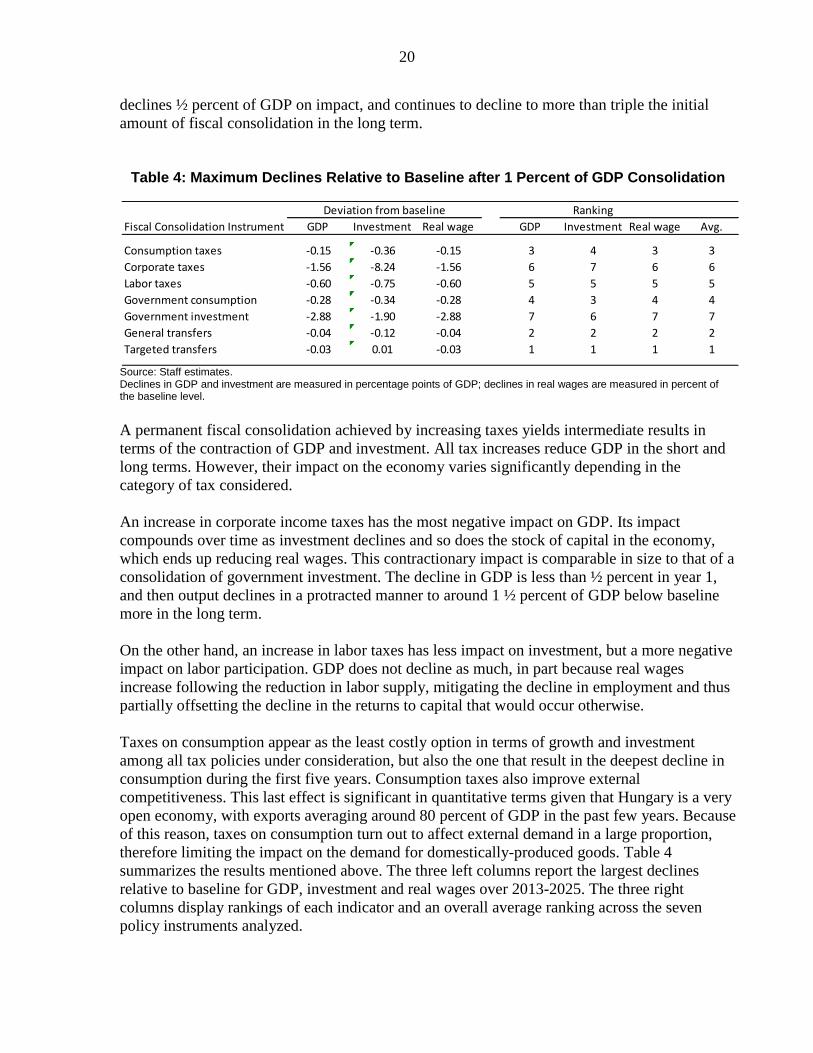
Table 4: Maximum Declines Relative to Baseline after 1 Percent of GDP Consolidation
Source: Staff estimates. Declines in GDP and investment are measured in percentage points of GDP; declines in real wages are measured in percent of the baseline level.
A permanent fiscal consolidation achieved by increasing taxes yields intermediate results in
terms of the contraction of GDP and investment. All tax increases reduce GDP in the short and
long terms. However, their impact on the economy varies significantly depending in the
category of tax considered.
An increase in corporate income taxes has the most negative impact on GDP. Its impact
compounds over time as investment declines and so does the stock of capital in the economy,
which ends up reducing real wages. This contractionary impact is comparable in size to that of a
consolidation of government investment. The decline in GDP is less than ½ percent in year 1,
and then output declines in a protracted manner to around 1 ½ percent of GDP below baseline
more in the long term.
On the other hand, an increase in labor taxes has less impact on investment, but a more negative
impact on labor participation. GDP does not decline as much, in part because real wages
increase following the reduction in labor supply, mitigating the decline in employment and thus
partially offsetting the decline in the returns to capital that would occur otherwise.
Taxes on consumption appear as the least costly option in terms of growth and investment
among all tax policies under consideration, but also the one that result in the deepest decline in
consumption during the first five years. Consumption taxes also improve external
competitiveness. This last effect is significant in quantitative terms given that Hungary is a very
open economy, with exports averaging around 80 percent of GDP in the past few years. Because
of this reason, taxes on consumption turn out to affect external demand in a large proportion,
therefore limiting the impact on the demand for domestically-produced goods. Table 4
summarizes the results mentioned above. The three left columns report the largest declines
relative to baseline for GDP, investment and real wages over 2013-2025. The three right
columns display rankings of each indicator and an overall average ranking across the seven
policy instruments analyzed.
Deviation from baseline Ranking
Fiscal Consolidation Instrument GDP Investment Real wage GDP Investment Real wage Avg.
Consumption taxes -0.15 -0.36 -0.15 3 4 3 3
Corporate taxes -1.56 -8.24 -1.56 6 7 6 6
Labor taxes -0.60 -0.75 -0.60 5 5 5 5
Government consumption -0.28 -0.34 -0.28 4 3 4 4
Government investment -2.88 -1.90 -2.88 7 6 7 7
General transfers -0.04 -0.12 -0.04 2 2 2 2
Targeted transfers -0.03 0.01 -0.03 1 1 1 1
21
An important issue to remark is that some of the fiscal consolidation policy instruments may
have a comparable impact on GDP growth, but their distributional (and social) consequences
can be very different. This is particularly so in the case of fiscal consolidation by increasing
taxes. A consolidation achieved with consumption and labor taxes tends to weigh more heavily
on households than a consolidation with corporate income taxes. However, it is important to
notice that this is less obvious when it comes to considering the distributional implications of
expenditure-based consolidations, as noted above.
The results above should be interpreted with caution, as they are subject to caveats. First, the
results are specific to the model set up and transmission channels assumed. This is a typical
caveat that applies to any model-based policy simulation. For example, Benk and Jacab (2012)
find that non-Keynesian effects may dominate over the contractionary forces of a fiscal
consolidation in the medium term. They show that, in order for a consolidation to be
expansionary, it is necessary to have a decline in the sovereign premium that reduces interest
rates further. Also, some channels potentially affecting growth are not modeled explicitly. For
example, if transfers to private agents (OLG and LIQ) affect investment in human capital such
as in health and education, then it is possible that the growth effects of a consolidation of
government transfers as predicted in the model are underestimated. Second, the results above
assume that the consolidation is fully credible after it is announced, meaning that all participants
in the economy internalize the policy change in full and anticipate no policy reversals or
implementation problems. This assumption is critical to the investment and output results
obtained, which are largely based on forward-looking behavior assumptions in a context of
rational (OLG) consumers and investors.

22
APPENDIX 1. DYNAMIC PARAMETERS CALIBRATIONS
Table A.1. Preferences and Population Related
HN EU RW
Elasticities of Substitution in Utility
Intertemporal (1/GAMMA) 0.5 0.5 0.5
Labor and Consumption
OLG Agents (ETA_OLG) 0.827 0.832 0.798
Elasticity of Labor Supply
OLG Agents 0.5 0.5 0.5
LIQ Agents 0.5 0.5 0.5
Other Structural Parameters
Habit Persistence (NU) 0.4 0.4 0.4
'Pure' Discount Factor (BBETA) 98.176 99.046 98.012
Probability of Survival (THETA) 0.95 0.95 0.95
Income Decline Rate (CHI) 0.95 0.95 0.95
Marginal Propensity to Consume (MPC) 4.522 4.665 4.974
Share of LIQ Agents (PSI) 0.3 0.3 0.4
23
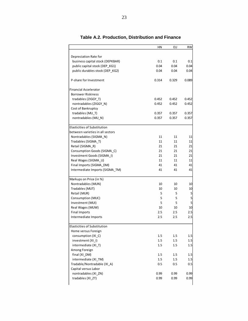
Table A.2. Production, Distribution and Finance
HN EU RW
Depreciation Rate for
business capital stock (DEPKBAR) 0.1 0.1 0.1
public capital stock (DEP_KG1) 0.04 0.04 0.04
public durables stock (DEP_KG2) 0.04 0.04 0.04
P-share for Investment 0.314 0.329 0.089
Financial Accelerator
Borrower Riskiness
tradables (ZIGGY_T) 0.452 0.452 0.452
nontradables (ZIGGY_N) 0.452 0.452 0.452
Cost of Bankruptcy
tradables (MU_T) 0.357 0.357 0.357
nontradables (MU_N) 0.357 0.357 0.357
Elasticities of Substitution
between varieties in all sectors
Nontradables (SIGMA_N) 11 11 11
Tradables (SIGMA_T) 11 11 11
Retail (SIGMA_R) 21 21 21
Consumption Goods (SIGMA_C) 21 21 21
Investment Goods (SIGMA_I) 21 21 21
Real Wages (SIGMA_U) 11 11 11
Final Imports (SIGMA_DM) 41 41 41
Intermediate Imports (SIGMA_TM) 41 41 41
Markups on Price (in %)
Nontradables (MUN) 10 10 10
Tradables (MUT) 10 10 10
Retail (MUR) 5 5 5
Consumption (MUC) 5 5 5
Investment (MUI) 5 5 5
Real Wages (MUW) 10 10 10
Final Imports 2.5 2.5 2.5
Intermediate Imports 2.5 2.5 2.5
Elasticities of Substitution
Home versus Foreign
consumption (XI_C) 1.5 1.5 1.5
investment (XI_I) 1.5 1.5 1.5
intermediate (XI_T) 1.5 1.5 1.5
Among Foreign
final (XI_DM) 1.5 1.5 1.5
intermediate (XI_TM) 1.5 1.5 1.5
Tradable/Nontradable (XI_A) 0.5 0.5 0.5
Capital versus Labor
nontradables (XI_ZN) 0.99 0.99 0.99
tradables (XI_ZT) 0.99 0.99 0.99
24
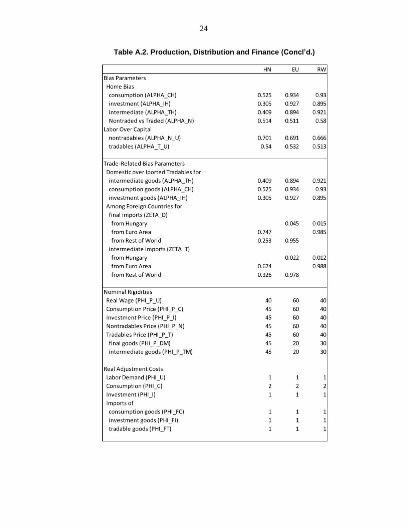
Table A.2. Production, Distribution and Finance (Concl’d.)
HN EU RW
Bias Parameters
Home Bias
consumption (ALPHA_CH) 0.525 0.934 0.93
investment (ALPHA_IH) 0.305 0.927 0.895
intermediate (ALPHA_TH) 0.409 0.894 0.921
Nontraded vs Traded (ALPHA_N) 0.514 0.511 0.58
Labor Over Capital
nontradables (ALPHA_N_U) 0.701 0.691 0.666
tradables (ALPHA_T_U) 0.54 0.532 0.513
Trade-Related Bias Parameters
Domestic over Iported Tradables for
intermediate goods (ALPHA_TH) 0.409 0.894 0.921
consumption goods (ALPHA_CH) 0.525 0.934 0.93
investment goods (ALPHA_IH) 0.305 0.927 0.895
Among Foreign Countries for
final imports (ZETA_D)
from Hungary 0.045 0.015
from Euro Area 0.747 0.985
from Rest of World 0.253 0.955
intermediate imports (ZETA_T)
from Hungary 0.022 0.012
from Euro Area 0.674 0.988
from Rest of World 0.326 0.978
Nominal Rigidities
Real Wage (PHI_P_U) 40 60 40
Consumption Price (PHI_P_C) 45 60 40
Investment Price (PHI_P_I) 45 60 40
Nontradables Price (PHI_P_N) 45 60 40
Tradables Price (PHI_P_T) 45 60 40
final goods (PHI_P_DM) 45 20 30
intermediate goods (PHI_P_TM) 45 20 30
Real Adjustment Costs
Labor Demand (PHI_U) 1 1 1
Consumption (PHI_C) 2 2 2
Investment (PHI_I) 1 1 1
Imports of
consumption goods (PHI_FC) 1 1 1
investment goods (PHI_FI) 1 1 1
tradable goods (PHI_FT) 1 1 1
25
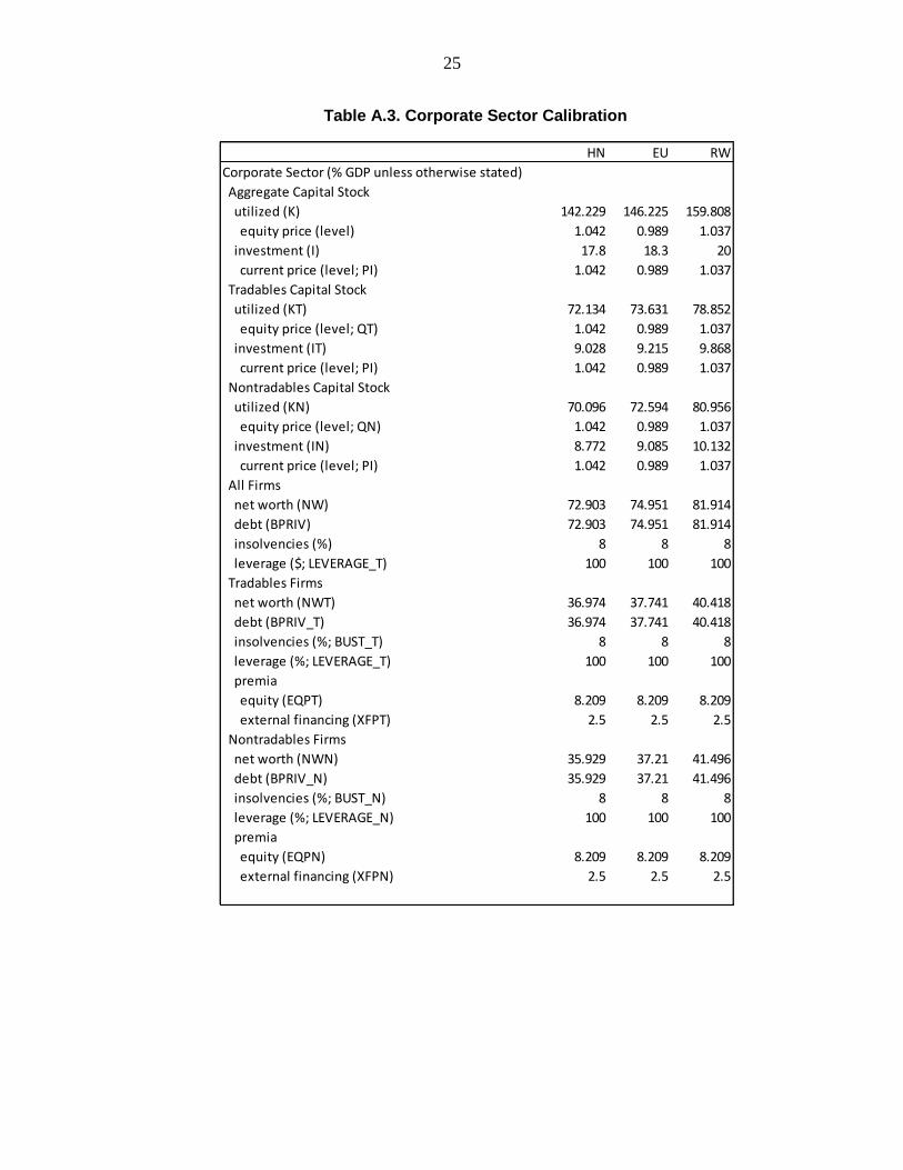
Table A.3. Corporate Sector Calibration
HN EU RW
Corporate Sector (% GDP unless otherwise stated)
Aggregate Capital Stock
utilized (K) 142.229 146.225 159.808
equity price (level) 1.042 0.989 1.037
investment (I) 17.8 18.3 20
current price (level; PI) 1.042 0.989 1.037
Tradables Capital Stock
utilized (KT) 72.134 73.631 78.852
equity price (level; QT) 1.042 0.989 1.037
investment (IT) 9.028 9.215 9.868
current price (level; PI) 1.042 0.989 1.037
Nontradables Capital Stock
utilized (KN) 70.096 72.594 80.956
equity price (level; QN) 1.042 0.989 1.037
investment (IN) 8.772 9.085 10.132
current price (level; PI) 1.042 0.989 1.037
All Firms
net worth (NW) 72.903 74.951 81.914
debt (BPRIV) 72.903 74.951 81.914
insolvencies (%) 8 8 8
leverage ($; LEVERAGE_T) 100 100 100
Tradables Firms
net worth (NWT) 36.974 37.741 40.418
debt (BPRIV_T) 36.974 37.741 40.418
insolvencies (%; BUST_T) 8 8 8
leverage (%; LEVERAGE_T) 100 100 100
premia
equity (EQPT) 8.209 8.209 8.209
external financing (XFPT) 2.5 2.5 2.5
Nontradables Firms
net worth (NWN) 35.929 37.21 41.496
debt (BPRIV_N) 35.929 37.21 41.496
insolvencies (%; BUST_N) 8 8 8
leverage (%; LEVERAGE_N) 100 100 100
premia
equity (EQPN) 8.209 8.209 8.209
external financing (XFPN) 2.5 2.5 2.5
26
REFERENCES
Baksa, B., Benk S., and Jacab Z., 2009, “Does “The” Fiscal Multiplier Exist? Fiscal and
Monetary Reactions, Credibility and Fiscal Multipliers in Hungary,” Office of the Fiscal
Council.
Barro, R.J., 1974), “Are Government Bonds Net Wealth?,” Journal of Political Economy, 82(6),
pp. 1097-1117.
Beetsma, R.M., and Jensen, H., 2005, “Monetary and Fiscal Policy Interactions in a Micro-
Founded Model of A Monetary Union,” Journal of International Economics, 67, pp.
320-352.
Benk, S. and Z. M. Jakab, 2012, “Non-Keynesian Effects of Fiscal Consolidation: An Analysis
with an Estimated DSGE Model for the Hungarian Economy,” OECD Economics
Department Working Papers, No. 945, pp. OECD.
Blanchard, O.J., 1985, “Debt, Deficits, and Finite Horizons,” Journal of Political Economy, No
93, pp. 223-247.
Blanchard, O. and Perotti, R., 2002, “An Empirical Characterization of the Dynamic Effects of
Changes in Government Deficits and Taxes on Output,” Quarterly Journal of
Economics, 117, pp. 1329-1368.
Blinder, A.S. 1981, “Temporary Income Taxes and Consumer Spending,” Journal of Political
Economy, 89(1), pp. 26-53.
Calvo, G.A. (1983), “Staggered Prices in a Utility-Maximizing Framework,” Journal of
Monetary Economics, No 12, pp. 383-398.
Coenen, G., Erceg, C., Freedman, C., Furceri, D., Kumhof, M., Lalonde, R., Laxton, D., Lindé,
J., Mourougane, A., Muir, D., Mursula, S., Roberts, J., Roeger, W., de Resende, C.,
Snudden S., Trabandt, M. and in’t Veld, J., 2010, “Effects of Fiscal Stimulus In
Structural Models,” IMF Working Paper 10/73 (Washington: International Monetary
Fund).
Faruqee, H., and Laxton, D., 2000, “Life-Cycles, Dynasties, Saving: Implications for Closed
and Small, Open Economies,” IMF Working Paper 00/216 (Washington: International
Monetary Fund)
27
Fatas, A., and Milhov, I. 2001, “The Effects of Fiscal Policy on Consumption and Employment:
Theory and Evidence,” CEPR Discussion Paper, No. 2060.
Gale, W., and Orszag, P., 2004, “Budget Deficits, National Saving, and Interest Rates,”
Brookings Papers on Economic Activity, No 2, pp. 101-187.
Horvath, A., Jacab Z., Kiss, G., and Parkanyi, B., 2006, “Myths and Maths: Macroeconomic
Effects of Fiscal Adjustments in Hungary,” Magyar Nemzeti Bank Occasional Papers
Series No. 52.
Ismayilov, I., 2011, “Unemployment Fiscal Multiplier and a Small Open Economy with Labor
Market Frictions,” Central European University paper series.
Kamps, C., 2004, “New Estimates of Government Net Capital Stocks for 22 OECD Countries
1960-2001,” IMF Working Paper 04/67 (Washington: International Monetary Fund).
Kumhof, M., and Laxton, D., 2007, “A Party Without a Hangover? On the Effects of U.S. Fiscal
Deficits,” IMF Working Paper 07/202 (Washington: International Monetary Fund).
_____, and Laxton, D., 2009a, “Simple, Implementable Fiscal Policy Rules,” IMF Working
Paper 09/76, (Washington: International Monetary Fund).
_____, 2009b, “Fiscal Deficits and Current Account Deficits,” IMF Working Paper 09/237,
(Washington: International Monetary Fund).
_____, Muir, D. And Mursula, S., 2010, “The Global Integrated Monetary and Fiscal Model
(GIMF) – Theoretical Structure,” IMF Working Paper 10/34 (Washington: International
Monetary Fund).
Laubach, T., 2003, “New Evidence on the Interest Rate Effects of Budget Deficits and Debt,”
Finance and Economics Discussion Series 2003-12, Board of Governors of the Federal
Reserve System.
Laxton, D., and Pesenti, P., 2003, “Monetary Rules for Small, Open, Emerging Economies,”
Journal of Monetary Economics, 50(5), pp. 1109-1152.
Ligthart, J.E., and Suárez, R.M.M. (2005), “The Productivity of Public Capital: A Meta
Analysis,” Working Paper, Tilburg University.
Mountford, A., and Uhlig, H. 2002, “What Are The Effects of Fiscal Policy Shocks?,” CEPR
Discussion Papers No. 3338.
Neumeyer, P.A., and Perri, F., 2004, “Business Cycles in Emerging Economies: The Role of
Interest Rates,” NBER Working Paper No. 10387.
28
Perotti, R., 2007, “In Search of the Transmission Mechanism of Fiscal Policy,” NBER Working
Papers No. 13143.
Rotemberg, J., 1982, “Sticky Prices in the United States,” Journal of Political Economy, 90,
1187-1211.
Schmitt-Grohe, S., and Uribe, M., 2007, “Optimal Simple and Implementable Monetary and
Fiscal Rules,” Journal of Monetary Economics, 54, pp. 1702-1725.
Seidman, L.S., 2003, Automatic Fiscal Policies to Combat Recessions (Armonk, New York:
M.E. Sharpe).
Solow, R.M., 2005, “Rethinking Fiscal Policy,” Oxford Review of Economic Policy, 21(4), pp.
509-514.
Talvi, E., and Vegh, C., 2005, “Tax Base Variability and Procyclical Fiscal Policy in
Developing Countries,” Journal of Development Economics, 78(1), pp. 156-190.
Taylor, J.B., 2000, “Reassessing Discretionary Fiscal Policy,” Journal of Economic
Perspectives, 14(3), pp. 21-36.