Embed Size (px)
Citation preview
The Computer ProgramFOURPT (Version 95.01) A Model for Simulating One-Dimensional, Unsteady, Open-Channel Flow
by Lewis L. DeLong, David B. Thompson, and Jonathan K. Lee
U.S. GEOLOGICAL SURVEY
Water-Resources Investigations Report 97-4016
Bay St. Louis, Mississippi 1997
DEPARTMENT OF THE INTERIOR
BRUCE BABBITT, Secretary
U.S. GEOLOGICAL SURVEY
GORDON P. EATON, Director
For additional information write to: Copies of this report can be purchased from:Project Chief Surface-Water Hydraulics Project U.S. Geological SurveyU.S. Geological Survey Branch of Information ServicesBuilding 2101 Box 25286Stennis Space Center, MS 39529 Denver, CO 80225-0286
Contents
Abstract 1
Introduction 2
Governing equations 3
Numerical solution 6
Numerical integration in time .................................. 8
Numerical integration in space ................................. 8
Linearization over a time step .................................. 9
Interpolation in space ...................................... 12
Direct matrix solution ...................................... 15
Computer code 16
Input 18
Program control ......................................... 18
Schematic description ...................................... 26
Channel properties ........................................ 30
Constraint properties ....................................... 35
Three-parameter constraint ................................ 35
User-programmable constraint............................... 37
File names and unit numbers .................................. 39
Initial values ........................................... 39
Boundary values ......................................... 42
Density values .......................................... 43
Perturbation parameters ..................................... 45
Output 48
General results .......................................... 48
Restart .............................................. 48
Space series ............................................ 48
Time series ............................................ 50
Examples 51
Example 1 - Steady flow in a channel with expanding width ................. 51
Example 2 - Unsteady flow in a prismatic channel ...................... 52
Example 3 - Diffusion and kinematic wave approximations ................. 54
Example 4 - Unsteady flow in a simple network of channels ................. 59
Example 5 - Applying user-programmed constraints ..................... 59
References 66
List of Figures
1 Computational grid. .................................... 6
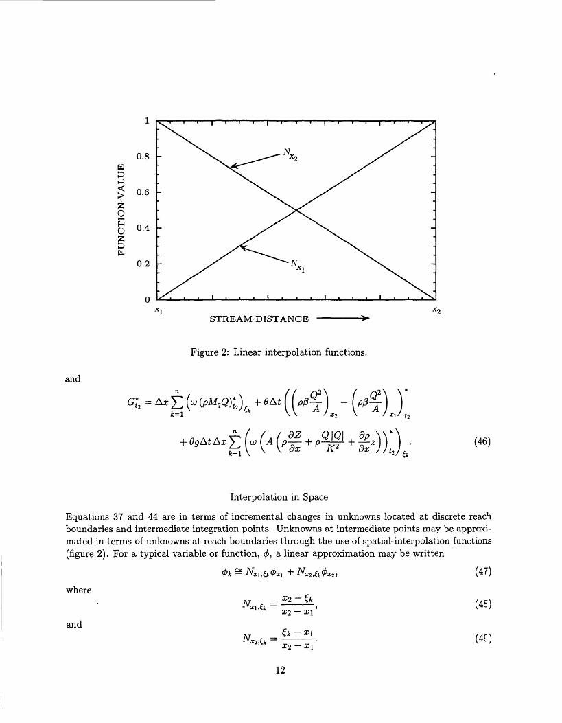
2 Linear interpolation functions. .............................. 12
3 Example program-control data file. ........................... 19
4 Sinusoidal component used in optional computation of boundary values from equations. 25
5 Partial example schematic-data file, four channels of a six-channel network. ..... 28
6 Example rectangular cross-section data file. ....................... 30
7 Example trapezoidal cross-section data file. ....................... 31
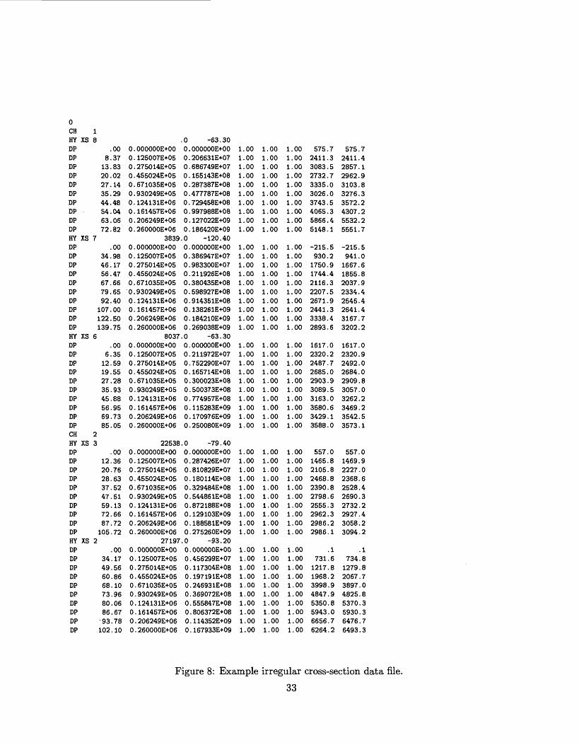
8 Example irregular cross-section data file. ........................ 33
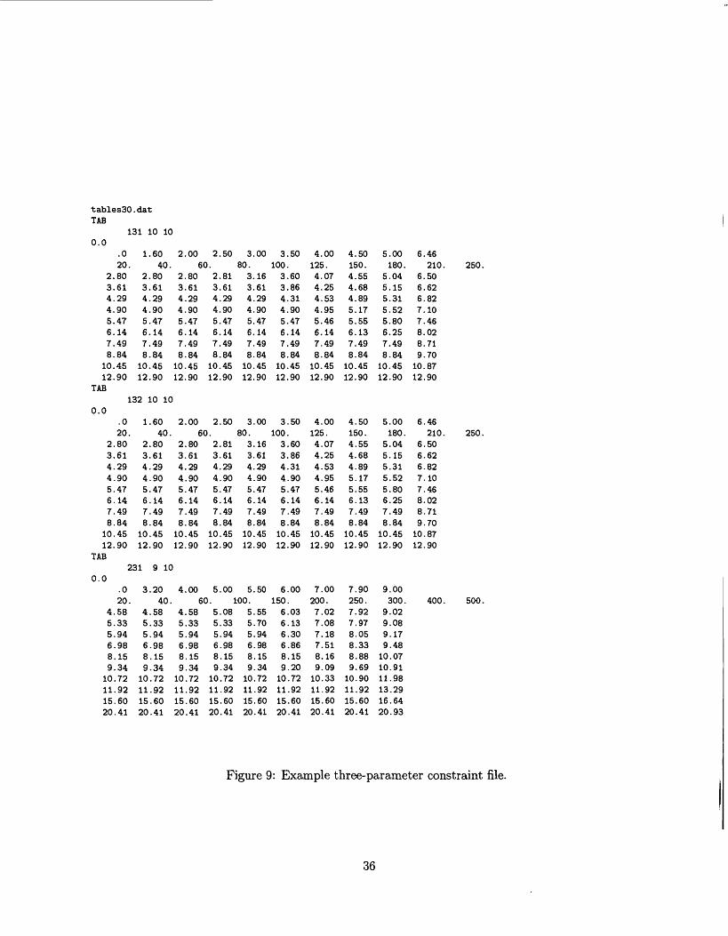
9 Example three-parameter constraint file. ........................ 36
10 Example master file-name and unit-number file. .................... 40
11 Example initial-values file. ................................ 41
12 Example boundary-values file. .............................. 43
13 Example density-values file for a two-channel network. ................ 44
iii
14 Example perturbation-parameter file. .......................... 45
15 Example general-results file. ............................... 49
16 Example tab-delimited space-series file. ......................... 50
17 Example tab-delimited time-series file. ......................... 50
18 Example-1 schematic-data file. .............................. 51
19 Spatial convergence in a channel with expanding width. ................ 52
20 Example-2 program-control-data file. .......................... 53
21 Example-2 schematic-data file. .............................. 54
22 Spatial and temporal convergence in a prismatic channel, at a location 50,000 ftdownstream. ........................................ 55
23 Impact of 0 on numerical convergence. ......................... 56
24 Comparison of dynamic- and diffusion-wave formulations on steady flow in the non- prismatic channel of example 1. ............................. 57
25 Failure of the kinematic approximation to reach steady flow when applied to thenonprismatic channel of example 1. ........................... 58
26 Different solution formulations and the prismatic channel section. .......... 58
27 Schematic representation of a simple six-channel network. ............... 59
28 Flow in a simple six-channel network. .......................... 60
29 Example-4 schematic-data file. .............................. 61
30 Example-4 schematic-data file continued. ........................ 62
31 Example-5 schematic-data file. .............................. 64
32 Example-5 constraint-properties file. ........................... 65
33 Inflow to reservoir and flow at dam for example 5. ................... 66
34 Relation of water-surface elevation to discharge for example 5 (first 20 hours ofsimulation). ........................................ 67
IV
List of Tables
1 FORTRAN 77 modules used in FoimPT. ........................ 17
2 Main-program and utility files used in FouaPT. .................... 17
3 Input files. ......................................... IP
4 Output files. ........................................ 4?
v
FACTORS FOR CONVERTING INCH-POUND UNITS TOINTERNATIONAL SYSTEM (SI) UNITS
Multiply inch-pound units By To obtain SI units foot (ft) 0.3048 meter mile (mi) 1.609 kilometer cubic foot per second (ft3 /8) 0.02832 cubic meter per second
VI
The Computer Program FOURPT(Version 95.01) a Model for Simulating
One-Dimensional, Unsteady, Open-Channel Flow
by Lewis L. DeLong, David B. Thompson, and Jonathan K. Lee
ABSTRACT
FOURPT is a computer program capable of computing unsteady one-dimensional flow in networks of open-channels. Optionally, governing equations may represent dynamic-wave, diffusion-wave, or kinematic-wave equations and may include variable channel sinuosity and variable water density. If density is allowed to vary, density values must be supplied by the user as this version of FOURPT does not currently compute transport or heat flow. Governing equations are converted to a set of linearized equations using a four-point-implicit finite-difference method with Newton-Raphron iteration. The resulting set of simultaneous equations are solved directly by Gaussian elimination.
Optional boundary conditions include known flow, water-surface elevation, water-surface slope, and three-parameter ratings. Additionally, a facility exists for users to program their own boundary constraints. Logarithmic and semi-logarithmic stage-discharge relations and dam-break functions also may be used as boundary constraints and are included in the program code as examples of user-programmed boundary constraints.
Channel cross sections may be represented by rectangular, trapezoidal, or irregular geometry, de pending on which geometry routines are linked with the program code. Spacing of user-suppl:c*i channel cross sections is independent of the selection of spatial discretization for numerical solution.
FOURPT is written in FORTRAN 77 using a data-encapsulation programming paradigm.
This report describes data input and output and demonstrates selected model capabilities with ex amples. The computer code and example data sets are available for electronic retrieval via World Wide Web from http://water.usgs.gov/software/FourPt.html or anonymous File Transfer Protocol from /pub/software/surface_water/FourPt.
INTRODUCTION
This report summarizes the formulation and use of FOURPT, version 95.01, a computer program for simulating one-dimensional, unsteady, open-channel flow. It is written in FORTRAN?? (American National Standards Institute 1978) using FORTRAN modules (DeLong, Thompson, and Fulforcf 1992; Thompson, DeLong, and Fulford 1992).
The primary purpose of version 95.01 is to provide a computer code capable of demonstrating nontrivial concepts important to the simulation of unsteady open-channel flow and yet is easy to read, modify, and run on a variety of computer systems. This report describes the governing equations, numerical formulation, computer code, input and output, and presents a set of examples selected to demonstrate concepts important to the numerical simulation of unsteady open-channe1 flow. The computer code and example data sets are available for electronic retrieval via World Wide Web from http: //water .usgs. gov/sof tware/FourPt. html or anonymous File Transfer Protocol from /pub/software/surface_water/FourPt.
Sections in this report cover distinct topics in a logical progression but may be referenced au tonomously. For example, a reader interested only in testing the FOURPT code on a specific computer might first refer to sections Computer Code and Input
GOVERNING EQUATIONS
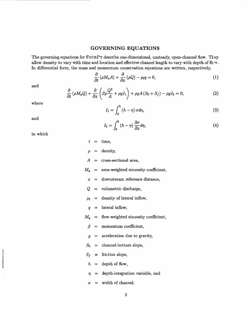
The governing equations for FOURPT describe one-dimensional, unsteady, open-channel flow. They allow density to vary with time and location and effective channel length to vary with depth of flew. In differential form, the mass and momentum conservation equations are written, respectively,
and
where
and
in which
%:(pMqQ) + jl-\J\J C/*/y
- (pMaA) + (PQ) - Piq = 0,
T + P9li + P9A (So + Sf ) - pgh = 0,
r=
Jo-rj) crdr),
daf da= J0 fi-rtte
(2)
(3)
(4)
t = time,
p = density,
A = cross-sectional area,
Ma = area-weighted sinuosity coefficient,
x = downstream reference distance,
Q = volumetric discharge,
Pi = density of lateral inflow,
q = lateral inflow,
Mq = flow-weighted sinuosity coefficient,
J3 = momentum coefficient,
g = acceleration due to gravity,
<$b = channel-bottom slope,
Sf = friction slope,
h = depth of flow,
77 = depth-integration variable, and
a = width of channel.
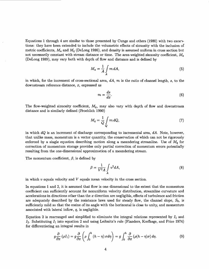
Equations 1 through 4 are similar to those presented by Cunge and others (1980) with two execu tions: they have been extended to include the volumetric effects of sinuosity with the inclusion of metric coefficients, Ma and Mq (DeLong 1986), and density is assumed uniform in cross section frit not necessarily constant with stream distance or time. The area-weighted sinuosity coefficient, Ma (DeLong 1989), may vary both with depth of flow and distance and is defined by
1 F Ma = -r / mdA, (5)
in which, for the increment of cross-sectional area, dA, m is the ratio of channel length, s, to the downstream reference distance, or, expressed as
ds ..
The flow- weighted sinuosity coefficient, Mg , may also vary with depth of flow and downstream distance and is similarly defined (Proehlich 1990)
dQ, (7) Q
in which dQ is an increment of discharge corresponding to incremental area, dA. Note, however, that unlike mass, momentum is a vector quantity, the conservation of which can not be rigorously enforced by a single equation describing motion along a meandering streamline. Use of Mq for correction of momentum storage provides only partial correction of momentum errors potentially resulting from the one-dimensional approximation of a meandering stream.
The momentum coefficient, /?, is defined by
in which v equals velocity and V equals mean velocity in the cross section.
In equations 1 and 2, it is assumed that flow is one dimensional to the extent that the momentum coefficient can sufficiently account for nonuniform velocity distribution, streamline curvature and accelerations in directions other than the x direction are negligible, effects of turbulence and friction are adequately described by the resistance laws used for steady flow, the channel slope, ,So, is sufficiently mild so that the cosine of its angle with the horizontal is close to unity, and momentum associated with lateral inflow, q, is negligible.
Equation 2 is rearranged and simplified to eliminate the integral relations represented by I\ and /2- Substituting I\ into equation 2 and using Leibnitz's rule (Flanders, Korfhage, and Price 1974) for differentiating an integral results in
d d fh \ fh d
Differentiating within the integral and rearranging terms results in
d [h d dp fh fh da 9Tx (ph) = gp ̂ a^ (h -n)dn + g-^ ̂ (ft - ) od, + gp ̂ (ft - ) -dr,, (10)
which reduces to
9-j^ (Pli) = 9pAfx + gA-g* + gph, (11)
where z is the distance from the water surface to the centroid of the cross section and is defined by
rh JO
Substituting equation 11 into equation 2 results in
(pMqQ) + TT- I flp r I + 9A { pSo ot ox \ A I \
Substituting the relationdh _ d.dx d
into equation 13 results in
where Z is the distance of the water surface above a common datum.
The flow resistance term, 5/, is replaced through substitution of the empirical relation
Q = Ky/S'f, (16)
where K is total channel conveyance, resulting in
The absolute value in equation 17 forces flow resistance to always oppose flow. Equation 17 is the equation governing momentum conservation in FOURPT.
*2
1111L
T 1111
J
t 1111 1Jl
XT Xo Xo Xi
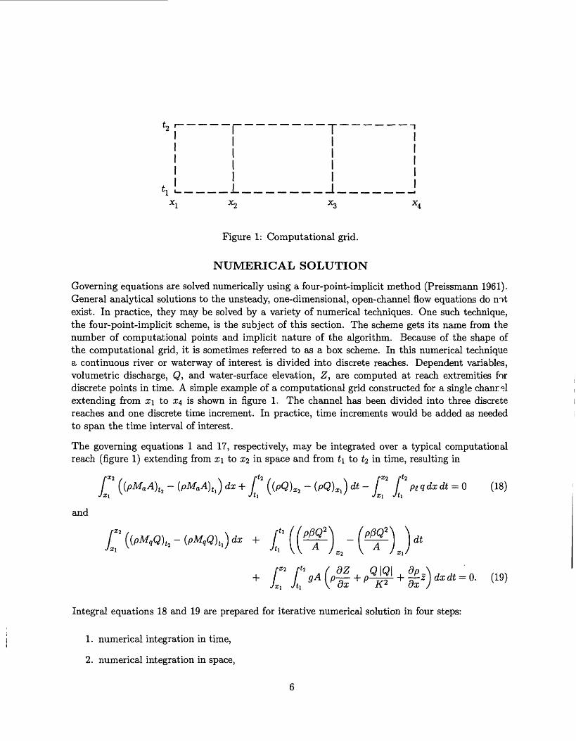
Figure 1: Computational grid.
NUMERICAL SOLUTION
Governing equations are solved numerically using a four-point-implicit method (Preissmann 1961). General analytical solutions to the unsteady, one-dimensional, open-channel flow equations do not exist. In practice, they may be solved by a variety of numerical techniques. One such technique, the four-point-implicit scheme, is the subject of this section. The scheme gets its name from the number of computational points and implicit nature of the algorithm. Because of the shape of the computational grid, it is sometimes referred to as a box scheme. In this numerical technique a continuous river or waterway of interest is divided into discrete reaches. Dependent variables, volumetric discharge, Q, and water-surface elevation, Z, are computed at reach extremities for discrete points in time. A simple example of a computational grid constructed for a single chanr^l extending from x\ to x\ is shown in figure 1. The channel has been divided into three discrete reaches and one discrete time increment. In practice, time increments would be added as needed to span the time interval of interest.
The governing equations 1 and 17, respectively, may be integrated over a typical computation al reach (figure 1) extending from x\ to xi in space and from t\ to ti in time, resulting in
and
r ((pMaA\2 - (pMaA) t } dx + I' ((pQ) X2 - (PQ) Xi ) dt - T [*piqdxdt = Q (18)Jx\ Jt\ Jxi Jt\
Integral equations 18 and 19 are prepared for iterative numerical solution in four steps:
1. numerical integration in time,
2. numerical integration in space,
3. linearization over a single iteration in terms of incremental change in dependent variables using approximations obtained from truncated Taylor series, and
4. spatial approximation in terms of dependent variables located specifically at computational- reach extremities.
More detailed presentation of these four steps is contained in the following four subsections. For the reach described by equations 18 and 19, the four steps result in determination of coefficients in a corresponding pair of linear equations
02,1 = B2
and
where, typical to all variables, charge at x\.
(20)
(21)
zj represents the incremental change, over an iteration, in
Assembly of equations resulting from similar operations on governing equations associated with all computational reaches along with appropriate boundary conditions results in a set of linear equations equal in number to the number of dependent variables,
ci.i02,1
C3,l C3,2 £3,3 03,4
C4,3 C4,4 04,5
C8,8 - AZI4
B3
B7
(22)
The equation set 22 is a simple example corresponding to the single channel schematized in figure 1. More complex networks of interconnected channels would, perhaps, result in hundreds to thousands of equations.
First and last rows of the equation set 22 are obtained from boundary conditions or constraints en forced at the extremities of each channel or branch of a network of channels. The simultaneous set of equations is solved directly for incremental change in dependent variables, dependent variables are adjusted by the incremental change, new coefficients are computed, and the process is repeated until the incremental change in dependent variables falls within acceptable limits. The solution £.1- gorithm then advances in time, and the iterative process is repeated for successive time increments. Values of dependent variables are determined at extremities of all computational reaches at points in time bounding each time increment. Derivation of expressions used to compute coefficients ard description of the method used to solve equation 22 are contained in the following five subsections.
Numerical Integration in Time
Numerical integration in time is accomplished through the use of a time-weighting parameter, 9. For a typical variable, 0,
0 = f (a?, z) (23)
time integration is accomplished by
<f>x t dt * (0 (<f>x\ +(1-0) (<f>x\ } At (24)fJt\
The weighting parameter 9 may vary from 0.5 to 1.0 in the four-point-implicit scheme 4. (Effect of 0 is demonstrated in example 2.) Applying similar numerical integration to equations 18 and 19 and moving values known at time t\ to the right-hand side results in
'2
(pMaA) tl dx
(pg(j) t dx (25) x " * /l i Jxi ' Jxi l
and
<->Numerical Integration in Space
Numerical integration in space is accomplished through the use of a more general quadrature thc.n previously used for time integration and, for a typical variable, 0, is expressed by
(27)fc=i ' *k
where a; is a weighting function similar in concept to 9 used in numerical integration over tim^. The number, n, and location, £&, of integration points and magnitude of corresponding weights in
general determine accuracy of the approximation. Weights, w^, must sum to 1,
k=i
and integration locations, &, must fall within the integration interval, in this instance,
xi < f < x2 .
Applying this form of spatial integration to equations 25 and 26 results in
and
1k=l
!
\\ / 12
I-
A;=l \ \ / 0:2
)^ - (PQ)X1 ) =
Az w (pMaA) - (1 - 0) At (PQ)I2 - (PQ) X1*=1 "
4- 0At Arc^ w feg)< + (1 - 0) At Arc w (peq) t (30)
I (31) &
Linearization Over a Time Step
Nonlinear terms in equations 30 and 31 are approximated with truncated Taylor series written in terms of incremental changes in dependent variables Q and Z. For a typical variable or function, the approximation may be expressed by
* ^*2 AO"" ^
where ,AZ = Zi2 - Z* (33)
AQ = Qt, - Q?a (34)
and the superscript "*" indicates evaluation using current values of unknowns obtained from the. preceding iteration.
Applying similar approximations to equation 30 results in
k=l \ \**K
+ 0At ((p (Q* + AQ))X2 - (p (Q* + AQ))^ = A, (35)
wheren
- (1-0) At/_^t \ \r u 'lljf.
n n
Ax £ (w (P£9) t2 ), + (1 - 0) At Ax ^ (w (peq) tl ) f (36) t i t i
Moving terms (equation 35) known from the preceding iteration to the right-hand side results in
., 4a = A'- E'» (37)
where
Similarly, nonlinear terms appearing in equation 31 may be approximated by
10
+ ^r vr "
anddp fdA A dz\\* krr /JONdx(dz* + ~dz)j ( }
Substituting approximations 39 through 43 into equation 31 and moving terms known from the preceding iteration to the right-hand side results in
n\
*a
I &
* \
+
'v / &
dP fdA = , A dz\\\*
= Ftl -G*t2 (44)
where
11 -'/ fc=l \ \ / X2
h
11
WD
0.8
0.6
0.4
0.2
STREAM-DISTANCE
and
<% =
Figure 2: Linear interpolation functions.
12
(46)
&
Interpolation in Space
Equations 37 and 44 are in terms of incremental changes in unknowns located at discrete reach boundaries and intermediate integration points. Unknowns at intermediate points may be approxi mated in terms of unknowns at reach boundaries through the use of spatial-interpolation functions (figure 2). For a typical variable or function, <£, a linear approximation may be written
where
and
£2 ~~
X2
(46)
(4£)
12
In matrix notation the approximation may be written
The spatial derivative of a typical variable represented by the linear interpolation functions may be approximated by
wherecWSi,& _ "" * feo\
a ' v oz/ ax X2 xiand
1-, (53)
and in matrix notation written as
Substituting the interpolation functions and the relation,
T
into equations 37 and 44 results in
dZ' U
andn e \ n / f r\ \r v * \
{AQ} + Ax^ f u(pQ-~^r ) {^}T 1K=l \ / £j(
13
z
= #,-<%. (57)
Accumulating terms in equations 56 and 57, coefficients in linear equations 20 and 21 may now b^ written as
c2,i = -0pzi,ta At, (58)
A ^{ ( Si, dA A dM»\ \ »rC2,2 = Az£ l u lpiMa + A-) ) Nxk=l \ ^ ^
+fc=l
C2 ,3 = ^Px2)t 2 At, (60)
A V^ / ( / »>r u- - A U V y± 0.) \ \ T,T \ //?1\c2 ,4 = A2:5Jlu;lp(Ma + A-± L \ NXA , (61)fc=l V V ^ ' J ii / £k
andD _ 1~) IP* (£Z f)\r><2 L>t\ &, (Owsfj
1 '2 v xfor the mass-conservation equation, and
n s
c3,i = Ax 53 ( w fc=i ^
§)*^x,) , (63)A / «9 / t
14
(65)
and
£3 = Ftl - G?2 (67)
for the momentum-conservation equation.
Direct Matrix Solution
The equation set 22 is solved directly by Gaussian elimination (Carnahan, Luther, and Wilkes 1969) using computer routines previously employed in another one-dimensional flow model, HYDRAUX (DeLong and Schoellhamer 1989).
Because the coefficient matrix is very sparse (very few locations in the coefficient matrix con tain nonzero terms), a technique is used to avoid unnecessary computer storage and computation. The virtual two-dimensional coefficient matrix is transformed into a one-dimensional array. Tl" Q. one- dimensional array stores only coefficients actually computed from equations and coefficients potentially computed during Gaussian elimination. Gaussian elimination is performed only on co efficients stored in the one-dimensional array . . . avoiding unnecessary computation on void locations in the sparse two-dimensional coefficient matrix.
15
COMPUTER CODE
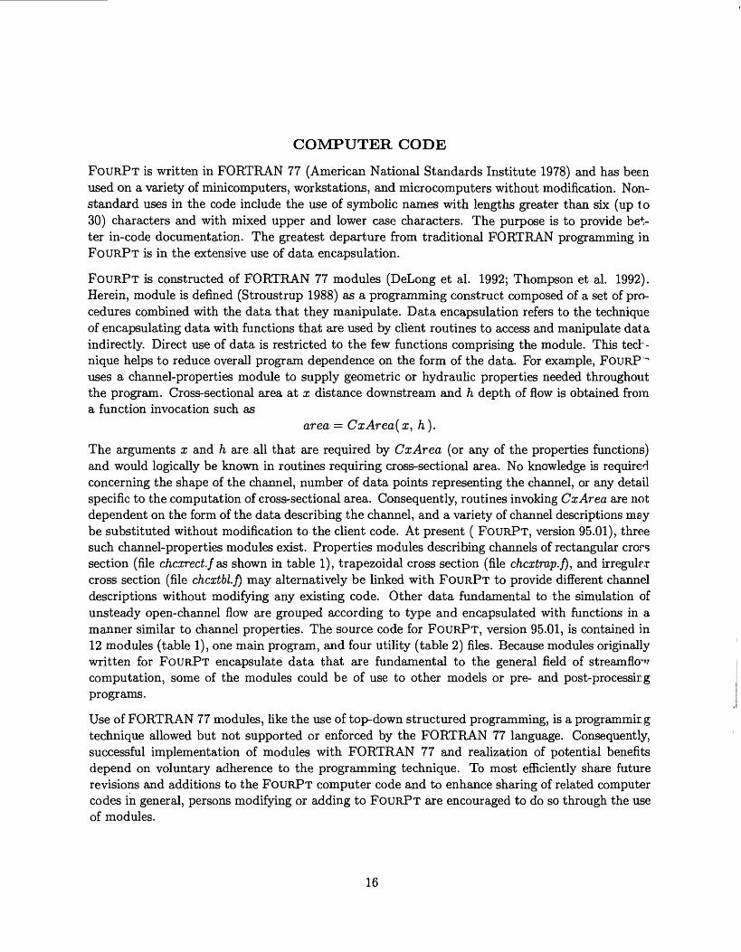
FoURPT is written in FORTRAN 77 (American National Standards Institute 1978) and has been used on a variety of minicomputers, workstations, and microcomputers without modification. Non- standard uses in the code include the use of symbolic names with lengths greater than six (up to 30) characters and with mixed upper and lower case characters. The purpose is to provide bet ter in-code documentation. The greatest departure from traditional FORTRAN programming in FoURPT is in the extensive use of data encapsulation.
FoURPT is constructed of FORTRAN 77 modules (DeLong et al. 1992; Thompson et al. 1992). Herein, module is defined (Stroustrup 1988) as a programming construct composed of a set of pro cedures combined with the data that they manipulate. Data encapsulation refers to the technique of encapsulating data with functions that are used by client routines to access and manipulate dat a indirectly. Direct use of data is restricted to the few functions comprising the module. This tech nique helps to reduce overall program dependence on the form of the data. For example, FOURP"" uses a channel-properties module to supply geometric or hydraulic properties needed throughout the program. Cross-sectional area at x distance downstream and h depth of flow is obtained from a function invocation such as
area = CxArea(x, h}.
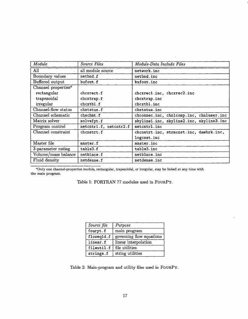
The arguments x and h are all that are required by CxArea (or any of the properties functions) and would logically be known in routines requiring cross-sectional area. No knowledge is required concerning the shape of the channel, number of data points representing the channel, or any detail specific to the computation of cross-sectional area. Consequently, routines invoking CxArea are not dependent on the form of the data describing the channel, and a variety of channel descriptions may be substituted without modification to the client code. At present ( FOURPT, version 95.01), three such channel-properties modules exist. Properties modules describing channels of rectangular crors section (file chcxrect.fas shown in table 1), trapezoidal cross section (file chcxtrap.f), and irregulr.r cross section (file chcxtbl.f) may alternatively be linked with FOURPT to provide different channel descriptions without modifying any existing code. Other data fundamental to the simulation of unsteady open-channel flow are grouped according to type and encapsulated with functions in a manner similar to channel properties. The source code for FOURPT, version 95.01, is contained in 12 modules (table 1), one main program, and four utility (table 2) files. Because modules originally written for FOURPT encapsulate data that are fundamental to the general field of streamfkr^ computation, some of the modules could be of use to other models or pre- and post-processing programs.
Use of FORTRAN 77 modules, like the use of top-down structured programming, is a programmirg technique allowed but not supported or enforced by the FORTRAN 77 language. Consequently, successful implementation of modules with FORTRAN 77 and realization of potential benefits depend on voluntary adherence to the programming technique. To most efficiently share future revisions and additions to the FOURPT computer code and to enhance sharing of related computer codes in general, persons modifying or adding to FOURPT are encouraged to do so through the use of modules.
16
Module Source Files Module-Data Include FilesAllBoundary valuesBuffered outputChannel properties0
rectangular trapezoidal irregular
Channel-flow statusChannel schematicMatrix solverProgram controlChannel constraint
Master file3-parameter ratingVolume/mass balanceFluid density
all module sourcenetbnd . fbuf out . f
chcxrect . f chcxtrap . f chcxtbl . fchstatus.fchschmt.fsolvef pt . fnetcntrl.f, netcntr2.fchcnstrt . f
master. ftables. fnetblnce . fnetdense . f
network . incnetbnd. incbuf out . inc
chcxrecl.inc, chcxrec2.inc chcxtrap. inc chcxtbl . incchstatus . incchconnec . inc , chnlcomp.inc, chnluser.incskylinel.inc, skyline2 . inc , skylineS.incnetcntrl . incchcnstrt . inc , strmcnst . inc , dambrk . inc , logcnst . incmaster . inctables. incnetblnce . incnetdense . inc
"Only one channel-properties module, rectangular, trapezoidal, or irregular, may be linked at any time with the main program.
Table 1: FORTRAN 77 modules used in FoimPT.
Source filef ourpt . ffloweqld.flinear. ffileutil.fstrings. f
Purposemain programgoverning flow equationslinear interpolationfile utilitiesstring utilities
Table 2: Main-program and utility files used in FOURPT.
17
Default filenamecontrol . datschemat.datcxgeom.datstrmcnst . datmaster. filinitcond.datbndval . datdensity.datperturb . dat
Data typeprogram controlschematic descriptionchannel propertiesconstraint propertiesfile names and unit numbersinitial valuesboundary valueswater density valuesperturbation parameters
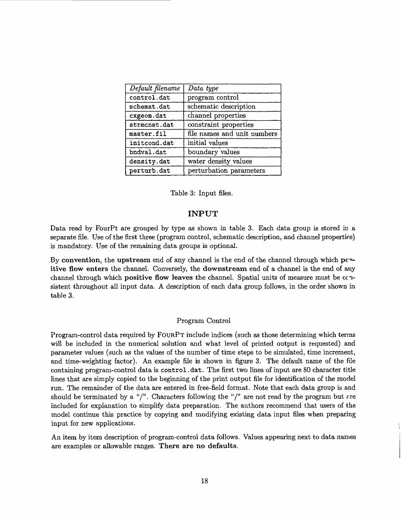
Table 3: Input files.
INPUT
Data read by FourPt are grouped by type as shown in table 3. Each data group is stored in a separate file. Use of the first three (program control, schematic description, and channel properties) is mandatory. Use of the remaining data groups is optional.
By convention, the upstream end of any channel is the end of the channel through which pc«- itive flow enters the channel. Conversely, the downstream end of a channel is the end of any channel through which positive flow leaves the channel. Spatial units of measure must be con sistent throughout all input data. A description of each data group follows, in the order shown in table 3.
Program Control
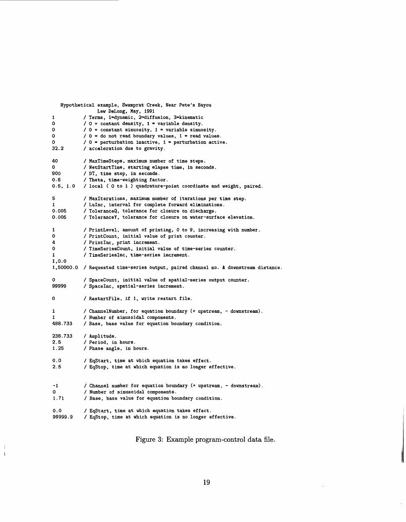
Program-control data required by FOURPT include indices (such as those determining which terms will be included in the numerical solution and what level of printed output is requested) and parameter values (such as the values of the number of time steps to be simulated, time increment, and time-weighting factor). An example file is shown in figure 3. The default name of the file containing program-control data is control. dat. The first two lines of input are 80 character title lines that are simply copied to the beginning of the print output file for identification of the model run. The remainder of the data are entered in free-field format. Note that each data group is and should be terminated by a "/". Characters following the "/" are not read by the program but rre included for explanation to simplify data preparation. The authors recommend that users of the model continue this practice by copying and modifying existing data input files when preparing input for new applications.
An item by item description of program-control data follows. Values appearing next to data names are examples or allowable ranges. There are no defaults.
18
Hypothetical example, Swamprat Creek, Near Pete's BayouLev DeLong, May, 1991
1 / Terms, l=dynamic, 2=diffusion, 3=kinematic0 / 0 = contant density, 1 » variable density.0 / 0 = constant sinuosity, 1 » variable sinuosity.0 / 0 = do not read boundary values, 1 » read values.0 / 0 * perturbation inactive, 1 » perturbation active.32.2 / acceleration due to gravity.
40 / MaxTimeSteps, maximum number of time steps.0 / NetStartTime, starting elapse time, in seconds.900 / DT, time step, in seconds.0.6 / Theta, time-weighting factor.0.5, 1.0 / local ( 0 to 1 ) quadrature-point coordinate and weight, paired.
5 / Maxlterations, maximum number of iterations per time step.1 / Lulnc, interval for complete forward eliminations.0.005 / ToleranceQ, tolerance for closure on discharge.0.005 / ToleranceY, tolerance for closure on water-surface elevation.
1 / PrintLevel, amount of printing, 0 to 9, increasing with number.0 / PrintCount, initial value of print counter.4 / Printlnc, print increment.0 / TimeSeriesCount, initial value of time-series counter.1 / TimeSeriesInc, time-series increment.1,0.01,50000.0 / Requested time-series output, paired channel no. & downstream distance.
0 / SpaceCount, initial value of spatial-series output counter.99999 / Spacelnc, spatial-series increment.
0 / RestartFile, if 1, write restart file.
1 / ChannelNumber, for equation boundary (+ upstream, - downstream).1 / Number of sinusoidal components.488.733 / Base, base value for equation boundary condition.
238.733 / Amplitude.2.5 / Period, in hours.1.25 / Phase angle, in hours.
0.0 / EqStart, time at which equation takes effect.2.5 / EqStop, time at which equation is no longer effective.
-1 / Channel number for equation boundary (+ upstream, - downstream).0 / Number of sinusoidal components.1.71 / Base, base value for equation boundary condition.
0.0 / EqStart, time at which equation takes effect.99999.9 / EqStop, time at which equation is no longer effective.
Figure 3: Example program-control data file.
19
Title lines:
Two 80-character lines of text that will be copied to the print output file. Use these lines to identify a particular model run.
Terms: 1, 2, or 3
This integer index determines which terms of the governing equations are included in the numerical solution, and consequently, whether the equations solved represent a
[1] dynamic-wave equation,
[2] diffusion-wave equation, or
[3] kinematic-wave equation.
For discussion of the above equations, see Example 3 under Examples. As a result of under lying physics, all equation types will not work correctly with all boundary conditions, initial conditions, or applications in general.
Density Index: 0 or 1
[0] density is assumed constant, or
[1] density is allowed to vary with space and time.
In the current version (95.01), if density is allowed to vary, for each time step a value of density must be supplied by the user for both ends of each channel. For a description of density input values, see Density Values under Input. In the absence of transport computations, density at intervening points is linearly estimated from values at channel ends.
Sinuosity Index: 0 or 1
[0] sinuosity is assumed constant with depth of flow, or
[1] sinuosity is allowed to vary with depth of flow.
Sinuosity, as used, is a ratio of channel length to main-valley length. As depth of flow increases in a natural meandering river, effective flow paths tend to shorten. Changes in effective channel length may significantly affect shape and speed of flood peaks. For more information regarding change in sinuosity with depth of flow, see DeLong (1986). Input of sinuosity as a function of flow depth is described for irregular cross sections under Channel Properties.
Boundary-Values Index: 0 or 1
[0] time varying boundary values will not be read, or
[1] boundary values will be read for each time step.
If the index is 1, boundary values must be supplied by the user in a separate boundary-value file. See Boundary Values under Input.
20
Perturbation Index: 0 or 1
[0] input data will not be randomly perturbed, or
[1] selected input data will be randomly perturbed.
In the current version (95.01), this option allows user to perturb coefficients used in boundary- value equations. The purpose of such perturbation might be to determine the relation of uncertainty in model results to uncertainty in boundary values. If this option is selected, the model will attempt to read normal-distribution parameters from a separate file with the default name perturb.dat. See Perturbation Parameters under Input.
Acceleration Due to Gravity: 32.2
This floating-point value represents the acceleration due to gravity. Spatial units should be consistent with other input such as initial conditions, boundary conditions, and schematic data. For example, 32.2 feet per second per second would be consistent with boundary and initial conditions entered in terms of cubic feet per second and feet. A value of 9.8 meters per second per second would be consistent with the use of cubic meter- per second and meters. Program output will be in the same units as input.
MaxTimeSteps: 0, 1, 2, ...oo
This integer value is the maximum number of time steps that will be simulated. It is limited only by available computer time or user perseverance. Total simulation time may be calculated
total simulation time = (MaxTimeSteps)(DT)
NetStartTime: -oo, 0, 1, 2, ...oo
This integer value is the starting elapsed time in seconds. Elapsed time at the end of a simulation may be calculated
ending elapse time = (MaxTimeSteps)(DT) + NetStartTime
DT: 1, 2, 3, ...oo
DT is the time increment, the length of a time step, in seconds. It is a positive, non-zerc, integer value. It should be small enough to adequately represent time dependent boundary conditions and simulated features of the flow (such as flood peaks). Adequacy of a selection and general sensitivity of results to DT should be determined by comparing results using a range of values for DT. Effects of DT and theta are interrelated. Additionally, the effects cf DT and spacing of computational cross sections (see Schematic Data) may be interrelated. Changes in DT will cause corresponding changes in the total simulated time. See definition of MaxTimeSteps given above.
Theta: 0.5 to 1.0, normally about 0.6
Theta, a floating-point value, is the time-weighting factor (see subsection Numerical Integra tion in Time under Numerical Formulation). Larger values of Theta numerically damp the
21
solution. A value of 0.5 represents equal time weighting of values and causes least numerical dampening of results. The effect of theta is related to length of the time step, DT, and is application dependent. Sensitivity of model results to theta and DT should be determined to avoid selection of values causing excessive numerical dampening. Use of Theta to dampen numerical oscillations occurring in results is not recommended. Numerical oscillations can generally be attributed to lack of numerical convergence with respect to space and or time and should be eliminated by appropriate adjustment of space and time increments.
Quadrature Points: 0.5, 1.0
A minimum of 1 to a maximum of 5 pairs of floating-point numbers represent, for each pair respectively, the location in local coordinates (0.0 to 1.0) and relative weight (0.0 to 1.0) to be given each point used in spatial integration. The example given above represents integration by evaluation at a point centered between end points of an interval and weighted by 1.0. If multiple integration points are used, their respective weights should sum to 1.0. Use of more than one integration point has not been shown to be advantageous but results in greater computational effort. Unless otherwise inclined for purpose of experimentation, users are advised to use the example values given above. This feature has been retained only for purpose of completeness and demonstration. More detailed discussion of numerical integration may be found in texts concerned with applied numerical techniques (Carnahan, Luther, and Wilkes 1969).
Maxlterations: 1, 2, 3, ...oo, normally about 5
This positive integer value is the maximum number of iterations allowed per time step. Few^r than the maximum may occur if the numerical scheme satisfies closure criteria. Generally, if a numerical scheme (FOURPT) does not satisfy closure criteria within 5 iterations, more iterations alone do not significantly improve results.
Lulnc: 1
This positive integer value relates to the algorithm for direct simultaneous solution of equa tions during model execution. It is the interval, in terms of iterations within a time step, at which complete forward elimination of the coefficient matrix will be performed. Intervening solutions will be computed with the coefficient matrix formed from a preceding iteration. Fcr- ward elimination automatically occurs on the first iteration of each time step. In general, more iterations will be required if a complete forward elimination is not performed every iteration. However, for large networks of channels, solutions without complete forward elimination for every iteration may require less overall execution time. The effect is problem dependent and specifically dependent on the relation of computational effort required for equation assembly to that required for subsequent forward elimination of the equations.
ToleranceQ: 0.005
This positive floating-point value is part of the closure criterion for flow. One of two separate criteria are exercised depending on whether the magnitude of the flow is larger or smaller than SmallQ, a value preset in the FOURPT computer code. If larger than SmallQ, computed flow at a location is considered to be sufficiently accurate when its magnitude of change over
22
the last iteration divided by its current value is equal to or less than ToleranceQ. If lers than or equal to SmallQ, computed flow at a location is considered to be sufficiently accurate when the magnitude of its change over the last iteration divided by SmallQ is equal to c^ less than ToleranceQ. SmallQ is preset equal to 100.0 in the FoURPx computer code. The overall solution for a time step is considered to have closed with respect to flow when the appropriate discharge criteria is satisfied at all computational locations.
ToleranceZ: 0.005
This positive floating-point value is part of the closure criterion for water-surface elevation. The computed water-surface elevation at a location is considered to be sufficiently accurate when the magnitude of the change in water-surface elevation over an iteration is smaller than ToleranceZ. The overall solution is considered to have closed with respect to water-surface elevation when the criteria is satisfied at all computational locations.
PrintLevel: 1
Positive integer sets the level of output written to the print file. Increasingly larger numbers produce increasing voluminous output:
[ 1] standard output (recommended).
[>1] adds schematic-data input and numbers of computational locations.
[>8] adds low-level debugging information regarding solution matrix.
PrintCount: 0
This integer value is the initial value of the print counter. For more information on how it may be used, see Printlnc below.
Printlnc: 0 to oo
This integer value is the interval, in time steps, at which printed output will be written during model execution. PrintCount is incremented by one at the beginning of each tirre step. At the conclusion of a time step, if PrintCount is equal to Printlnc, user-requested output ( see PrintLevel above ) is written to the print output file and PrintCount is set to zero.
TimeSeriesCount: 0
This integer value is the the initial value of the time-series output counter. For more info''- mation on how it may be used, see TimeSeriesInc below.
TimeSeriesInc: 1 to oo
This integer value is the interval, in time steps, at which time-series output will be saved during model execution, TimeSeriesCount is incremented by one at the beginning of each time step. At the conclusion of a time step, if TimeSeriesCount is equal to TimeSeriesIn0., timeseries output is stored in the time-series output file and TimeSeriesCount is set to zero. See Time-series locations below.
23
Time-series locations: 1, 0.0, 1, 50000.0
These values are paired channel number (integer value) and downstream distance (floating point value) specifying locations at which time-series of flow and water-surface elevation^ are to be saved. The maximum number of time series allowed is equal to MaxTS, set in the include file netcntrl. inc. In the example above, time series are requested at 0.0 and 50000.0 feet in channel 1. Channel-location pairs may be entered on more than one line. If no time series are requested, a line should still be entered and terminated with a "/".
SpaceCount: 0
This integer value is the initial value of the spatial-series output counter. For more information on how it may be used, see Spacelnc below.
Spacelnc: 1 to oo
This integer value is the interval, in time steps, at which spatial-series of flow and flow depth** will be saved during model execution. SpaceCount is incremented by one at the beginning of each time step. At the conclusion of a time step, if SpaceCount is equal to Spacelnc, spatial-series output is stored, and SpaceCount is set to zero.
RestartFile: 0
[0] Restart file is not requested.
[1] Restart file is requested.
A restart file contains values of flow and water-surface elevation that may subsequently be used as FOURPT initial conditions. To use the restart file for initial conditions, the correct initial condition flags must be set (see Schematic Data), and the file must be named appropriately (see File Names and Unit Numbers). If, when used, computational locations in the initial- condition file match those set in the current execution of FOURPT, values from the initial - condition file are used directly. If locations do not match, values at required locations ar? linearly interpolated from those contained in the initial-condition file.
The remainder of lines in the program-control file are optional and provide one of two methods for setting boundary values at channel extremities. The method described here is to estimate boundary values from equations with user-supplied parameters. A second method that involves reading a tim? series of boundary values from a user-supplied file is described in the section Boundary Values under Input When values are available from both sources for a specific boundary, values read from the time series are used.
Data required for the computation of boundary values from equations are parameters and coeffi cients related to the general harmonic equation
__ . _ _ 9 °^me s ( (ElapseTime + PhaseAnglei)\ ,._ N Value = EqBase + > Amplitude^ cos 2?r- - - £_H. ) (68)f-f V Penodi J
24
0 0.5 1 1.5 2 2.5 3TIME,--IN--HARMONIC COMPONENT-PERIODS
Figure 4: Sinusoidal component used in optional computation of boundary values from equations
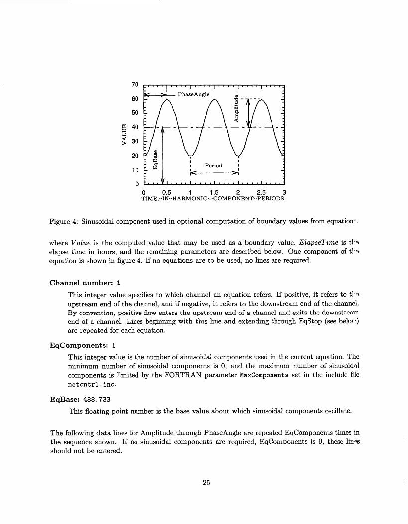
where Value is the computed value that may be used as a boundary value, ElapseTime is tl ^ elapse time in hours, and the remaining parameters are described below. One component of tH equation is shown in figure 4. If no equations are to be used, no lines are required.
Channel number: 1
This integer value specifies to which channel an equation refers. If positive, it refers to tH upstream end of the channel, and if negative, it refers to the downstream end of the channel. By convention, positive flow enters the upstream end of a channel and exits the downstream end of a channel. Lines beginning with this line and extending through EqStop (see belov) are repeated for each equation.
EqComponents: 1
This integer value is the number of sinusoidal components used in the current equation. The minimum number of sinusoidal components is 0, and the maximum number of sinusoidal components is limited by the FORTRAN parameter MaxComponents set in the include file netcntrl.inc.
EqBase: 488.733
This floating-point number is the base value about which sinusoidal components oscillate.
The following data lines for Amplitude through PhaseAngle are repeated EqComponents times in the sequence shown. If no sinusoidal components are required, EqComponents is 0, these lin^s should not be entered.
25
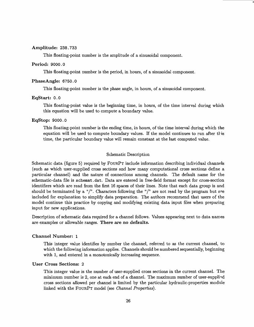
Amplitude: 238.733
This floating-point number is the amplitude of a sinusoidal component.
Period: 9000.0
This floating-point number is the period, in hours, of a sinusoidal component.
PhaseAngle: 6750.0
This floating-point number is the phase angle, in hours, of a sinusoidal component.
EqStart: 0.0
This floating-point value is the beginning time, in hours, of the time interval during which this equation will be used to compute a boundary value.
EqStop: 9000.0
This floating-point number is the ending time, in hours, of the time interval during which the equation will be used to compute boundary values. If the model continues to run after this time, the particular boundary value will remain constant at the last computed value.
Schematic Description
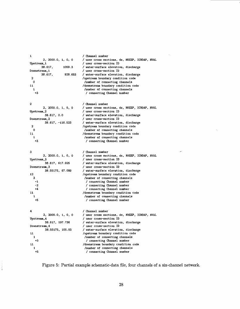
Schematic data (figure 5) required by FOURPT include information describing individual channels (such as which user-supplied cross sections and how many computational cross sections define a particular channel) and the nature of connections among channels. The default name for the schematic-data file is schemat.dat. Data are entered in free-field format except for cross-section identifiers which are read from the first 16 spaces of their lines. Note that each data group is and should be terminated by a "/". Characters following the "/" are not read by the program but are included for explanation to simplify data preparation. The authors recommend that users of the model continue this practice by copying and modifying existing data input files when preparing input for new applications.
Description of schematic data required for a channel follows. Values appearing next to data names are examples or allowable ranges. There are no defaults.
Channel Number: 1
This integer value identifies by number the channel, referred to as the current channel, to which the following information applies. Channels should be numbered sequentially, beginning with 1, and entered in a monotonically increasing sequence.
User Cross Sections: 2
This integer value is the number of user-supplied cross sections in the current channel. The minimum number is 2, one at each end of a channel. The maximum number of user-supplied cross sections allowed per channel is limited by the particular hydraulic-properties module linked with the FOURPT model (see Channel Properties).
26
dx: 2000.0
This floating-point value is the requested spacing, in feet, among computational cross sections. Actual spacing may be larger than dx in order to obtain an integer number of computational cross sections.
NKEEP: 0 or 1, normally 1
This integer index specifies that computational cross sections
[0] will not, or
[1] will
be placed at all locations occupied by user-supplied cross sections. During model runs, un knowns (such as water-surface elevation and flow) are located only at computational crors sections. This means that if NKEEP = 0, the only two user cross sections at which it can be ensured that unknowns will be determined will be those cross sections located at the extremities of the channel. All user-supplied cross sections would still be used for determir- ing geometric and hydraulic properties at computational cross sections and in intervening reaches. When using NKEEP = 0, particular attention should be addressed to checking spatial convergence of solutions.
ICNDAP: 0 to 7, only options 0, 1, 5, and 7 are currently implemented.
Integer indicates the type of approximation to be used for determining initial values of ur- knowns in the absence of observed values or values obtained from previous model runs. Initial conditions will be approximated from
[0] user input in schematic-data file,
[1] normal depth computations,
[2] (this option not assigned),
[3] same as 1, but channel filled to remove adverse slopes,
[4] maximum water-surface elevation for each channel,
[5] initial values file,
[6] not approximated, or
[7] steady flow computation within a channel.
For normal depth computations, option 1, water-surface elevation is approximated using initial flow values entered in the schematic-data file. For steady flow approximation, option 7, computations begin with the flow and water-surface elevation specified (in the schematic data file) at the downstream end of the channel and proceed upstream.
NVAL: 0
This index is reserved for future use.
27
2, 2000.0, 1, 0, 0 Upstream.1
38.617, 1059.3 Downstream.1
38.617, 928.653 20
11 1 +3
/ Channel number/ user cross sections, dx,/ user cross-section ID/ water-surface elevation,/ user cross-section ID/ water-surface elevation,/upstream boundary condition code/number of connecting channels
/downstream boundary condition code/number of connecting channels / connecting Channel number
NKEEP, ICNDAP, NVAL
discharge
discharge
2, 2000.0, 1, 0, 0 Upstream_2
38.617, 0.0 Downstream_2
38.617, -116.523 20
11 1 +3
/ Channel number/ user cross sections, dx, NKEEP, ICNDAP, NVAL/ user cross-section ID/ water-surface elevation, discharge/ user cross-section ID/ water-surface elevation, discharge/upstream boundary condition code/number of connecting channels
/downstream boundary condition code/number of connecting channels / connecting Channel number
2, 2000.0, 1, 0, 0 Upstream_3
38.617, 617.925 Downstream_3
38.55175, 67.089 12
3-1-2 +4
11
+5
/ Channel number/ user cross sections, dx/ user cross-section ID/ water-surface elevation/ user cross-section ID/ water-surface elevation/upstream boundary condition code/number of connecting channels/ connecting Channel number/ connecting Channel number/ connecting Channel number
/downstream boundary condition code /number of connecting channels / connecting Channel number
NKEEP, ICNDAP, NVAL
discharge
discharge
2, 2000.0, 1, 0, 0 Upstream_4
38.617, 197.736 Downstream_4
38.55175, 105.93 11
1+3
11 1 +5
/ Channel number/ user cross sections, dx, NKEEP, ICNDAP, NVAL/ user cross-section ID/ water-surface elevation, discharge/ user cross-section ID/ water-surface elevation, discharge/upstream boundary condition code/number of connecting channels/ connecting Channel number
/downstream boundary condition code/number of connecting channels / connecting Channel number
Figure 5: Partial example schematic-data file, four channels of a six-channel network.
28
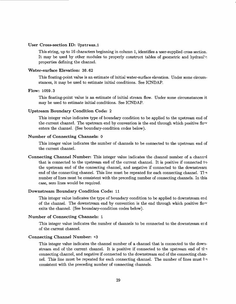
User Cross-section ID: Upstream_l
This string, up to 16 characters beginning in column 1, identifies a user-supplied cross section. It may be used by other modules to properly construct tables of geometric and hydrauPc properties defining the channel.
Water-surface Elevation: 38.62
This floating-point value is an estimate of initial water-surface elevation. Under some circum stances, it may be used to estimate initial conditions. See ICNDAP.
Flow: 1059.3
This floating-point value is an estimate of initial stream flow. Under some circumstances it may be used to estimate initial conditions. See ICNDAP.
Upstream Boundary Condition Code: 2
This integer value indicates type of boundary condition to be applied to the upstream end of the current channel. The upstream end by convention is the end through which positive fkrv enters the channel. (See boundary-condition codes below).
Number of Connecting Channels: 0
This integer value indicates the number of channels to be connected to the upstream end of the current channel.
Connecting Channel Number: This integer value indicates the channel number of a channel that is connected to the upstream end of the current channel. It is positive if connected to the upstream end of the connecting channel, and negative if connected to the downstream end of the connecting channel. This line must be repeated for each connecting channel. TI Q. number of lines must be consistent with the preceding number of connecting channels. In this case, zero lines would be required.
Downstream Boundary Condition Code: 11
This integer value indicates the type of boundary condition to be applied to downstream en d of the channel. The downstream end by convention is the end through which positive flo^^ exits the channel. (See boundary-condition codes below).
Number of Connecting Channels: 1
This integer value indicates the number of channels to be connected to the downstream er d of the current channel.
Connecting Channel Number: +3
This integer value indicates the channel number of a channel that is connected to the down stream end of the current channel. It is positive if connected to the upstream end of tb°. connecting channel, and negative if connected to the downstream end of the connecting chan nel. This line must be repeated for each connecting channel. The number of lines must b°. consistent with the preceding number of connecting channels.
29
1 / output index ( 0 - no echo, 1 - echo ).
1 / channel number.0.045 / flow resistance coefficient.Upstream_l / upstream cross-section identifier.0.0 100.0 100.0 / downstream distance, width, bottom elevation.Downstream_l / downstream cross-section identifier.50000.0 100.0 50.0 / downstream distance, width, bottom elevation.
2 / channel number.0.045 / flow resistance coefficient.Upstream_2 / upstream cross-section identifier.0.0 100.0 50.0 / downstream distance, width, bottom elevation.Downstream_2 / downstream cross-section identifier.50000.0 100.0 0.0 / downstream distance, width, bottom elevation.
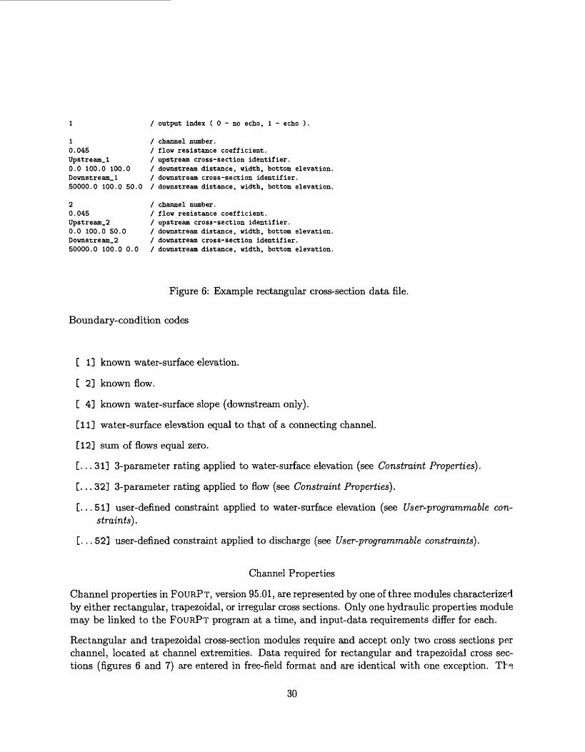
Figure 6: Example rectangular cross-section data file.
Boundary-condition codes
[ 1] known water-surface elevation.
[ 2] known flow.
[ 4] known water-surface slope (downstream only).
[11] water-surface elevation equal to that of a connecting channel.
[12] sum of flows equal zero.
[... 31] 3-parameter rating applied to water-surface elevation (see Constraint Properties).
[... 32] 3-parameter rating applied to flow (see Constraint Properties).
[...51] user-defined constraint applied to water-surface elevation (see User-programmable con straints).
[... 52] user-defined constraint applied to discharge (see User-programmable constraints).
Channel Properties
Channel properties in FOURPT, version 95.01, are represented by one of three modules characterized by either rectangular, trapezoidal, or irregular cross sections. Only one hydraulic properties module may be linked to the FOURPT program at a time, and input-data requirements differ for each.
Rectangular and trapezoidal cross-section modules require and accept only two cross sections per channel, located at channel extremities. Data required for rectangular and trapezoidal cross sec tions (figures 6 and 7) are entered in free-field format and are identical with one exception. The
30
1 / output index ( 0 - no echo, 1 - echo ).
1 / channel number.0.045 / flow resistance coefficient.Upstream_l / upstream cross-section identifier.0.0 100.0 10.0 1.0 / downstream distance, bottom width, bottom elevation,d(width)/dh.Downstream,1 / downstream cross-section identifier.5000.0 100.0 5.0 1.2 / downstream distance, bottom width, bottom elevation, d(width)/dh.
2 / channel number.0.045 / flow resistance coefficient.Upstream_2 / upstream cross-section identifier.5000.0 100.0 5.0 0.5 / downstream distance, bottom width, bottom elevation, d(width)/dh.
Downstream_2 / downstream cross-section identifier.9000.0 100.0 0.0 0.8 / downstream distance, bottom width, bottom elevation, d(width)/dh.
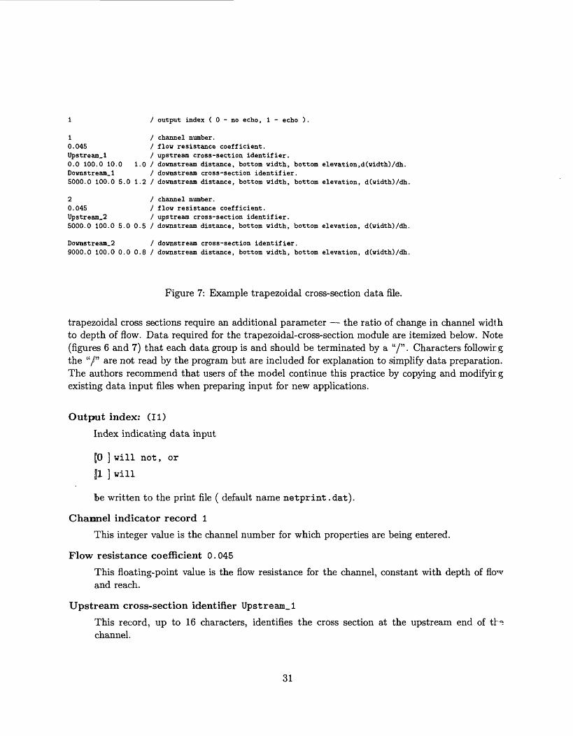
Figure 7: Example trapezoidal cross-section data file.
trapezoidal cross sections require an additional parameter the ratio of change in channel width to depth of flow. Data required for the trapezoidal-cross-section module are itemized below. Note (figures 6 and 7) that each data group is and should be terminated by a "/" Characters followirg the "/" are not read by the program but are included for explanation to simplify data preparation. The authors recommend that users of the model continue this practice by copying and modifying existing data input files when preparing input for new applications.
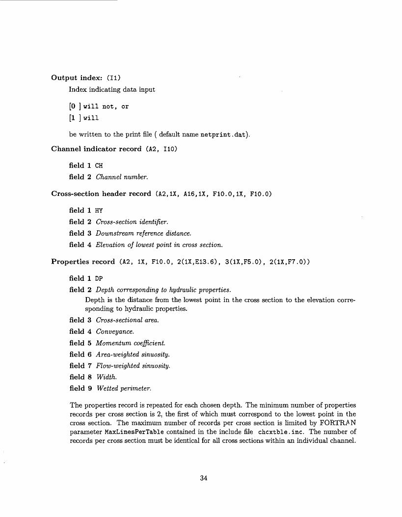
Output index: (II)
Index indicating data input
[0 ] will not, or
fl ] will
be written to the print file ( default name netprint .dat).
Channel indicator record 1
This integer value is the channel number for which properties are being entered.
Flow resistance coefficient 0. 045
This floating-point value is the flow resistance for the channel, constant with depth of fkrv and reach.
Upstream cross-section identifier Upstream. 1
This record, up to 16 characters, identifies the cross section at the upstream end of tN channel.
31
Upstream properties record 0.0 100.0 10.0 1.0
field 10.0
This floating-point value is the downstream reference distance.
field 2 100.0This floating-point value is the bottom width of the upstream cross section.
field 3 10.0This floating-point value is the elevation of the bottom of the upstream cross section.
field 4 1.0This floating-point value is the ratio of change in channel width with respect to depthin the upstream cross section.
Downstream cross-section identifier Downstream. 1
This record, up to 16 characters, identifies the cross section at the downstream end of the channel.
Downstream properties record 5000.0 100.0 0.5 1.2
field 1 5000.0This floating-point value is the downstream reference distance.
field 2 100.0This floating-point value is the bottom width of the downstream cross section.
field 35.0This floating-point value is the elevation of the bottom of the downstream cross section.
field 41.2This floating-point value is the ratio of change in channel width with respect to depthin the downstream cross section.
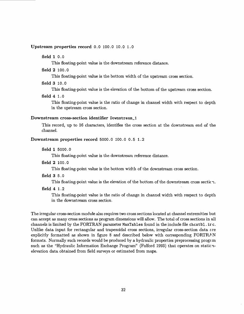
The irregular cross-section module also requires two cross sections located at channel extremities but can accept as many cross sections as program dimensions will allow. The total of cross sections in all channels is limited by the FORTRAN parameter MaxTables found in the include file chcxtbl .ire. Unlike data input for rectangular and trapezoidal cross sections, irregular cross-section data g.re explicitly formatted as shown in figure 8 and described below with corresponding FORTRAN formats. Normally such records would be produced by a hydraulic properties preprocessing prog£.m such as the "Hydraulic Information Exchange Program" (Fulford 1993) that operates on staticn- elevation data obtained from field surveys or estimated from maps.
32
0 CHHY XSDPDPDPDPDPDPDPDPDPDPHY XSDPDPDPDPDPDPDPDPDPDPHY XSDPDPDPDPDPDPDPDPDPDPCHHY XSDPDPDPDPDPDPDPDPDPDPHY XSDPDPDPDPDPDPDPDPDPDP
18
8.13.20.27.35.44.54.63.72.
7
34.46.56.67.79.92.
107.122.139.
6
6.12.19.27.35.45.56.69.85.
23
12.20.28.37.47.59,72.87.
105.2
3449,606873808693102
00378302142948040682
00981747666540005075
00355955289388957305
003676635251.1366.72.72
.00
.17
.56
.86
.10
.96
.06
.67
.78
.10
0.0.0.0.0.0.0.0.0.0.
0.0.0.0.0.0.0.0.0.0.
0.0.0.0.0.0.0.0.0.0.
0.0.0.0.0.0.0.0.0.0.
000,0000000
OOOOOOE+00125007E+05275014E+05455024E+05671035E+05930249E+05124131E+06161457E+06206249E+06260000E+06
3839.OOOOOOE+00125007E+05275014E+05455024E+05671035E+05930249E+05124131E+06161457E+06206249E+06260000E+06
8037.OOOOOOE+00125007E+05275014E+05455024E+05671035E+05930249E+05124131E+06161457E+06206249E+06260000E+06
22538,OOOOOOE+00
. 125007E+05. 275014E+05455024E+05.671035E+05.930249E+05. 124131E+06161457E+06
, 206249E+06. 260000E+06
27197. OOOOOOE+00. 125007E+05. 275014E+05.455024E+05.671035E+05.930249E+05. 124131E+06.161457E+06. 206249E+06.260000E+06
0 -63.300. OOOOOOE+000. 20663 1E+070.686749E+070.155143E+080.287387E+080.477787E+080.729458E+080.997988E+080.127022E+090.186420E+090 -120.400. OOOOOOE+000.386947E+070.983300E+070.211926E+080.380435E+080.598927E+080.914351E+080.138261E+090.184210E+090.269038E+09,0 -63.300 . OOOOOOE+000.211972E+070.752290E+070.165714E+080.300023E+080.500373E+080.774957E+080.115283E+090.170976E+090.250080E+09
.0 -79.400. OOOOOOE+000.287426E+070.810829E+070.180114E+080.329484E+080. 54486 1E+080.872188E+080.129103E+090.1 8858 1E+090 . 275260E+09.0 -93.200. OOOOOOE+000.456299E+070.117304E+080.197 19 1E+080. 24693 1E+080.369072E+080.555847E+080.806372E+080.114352E+090.167933E+09
1.001.001.001.001.001.001.001.001.001.00
1.001.001.001.001.001.001.001.001.001.00
1.001.001.001.001.001.001.001.001.001.00
1.001.001.001.001.001.001.001.001.001.00
1.001.001.001.001.001.001.001.001.001.00
1.001.001.001.001.001.001.001.001.001.00
1.001.001.001.001.001.001.001.001.001.00
1.001.001.001.001.001.001.001.001.001.00
1.001.001.001.001.001.001.001.001.001.00
1.001.001.001.001.001.001.001.001.001.00
1.001.001.001.001.001.001.001.001.001.00
1.001.001.001.001.001.001.001.001.001.00
1.001.001.001.001.001.001.001.001.001.00
1.001.001.001.001.001.001.001.001.001.00
1.001.001.001.001.001.001.001.001.001.00
575.2411.3083.2732.3335.3026.3743.4065.5866.5148.
-215.930.1750.1744.2116.2207.2671.2441.3338.2893.
1617.2320.2487.2685.2903.3089.3163.3580.3429.3588.
557.1465.2105.2468.2390.2798,2555,2962.2986,2986,
73112171968399848475350594366566264
7357005341
5294359346
0270,950,610
0,8.8,8.8.6.3.3.2.1
.1
.6
.8
.2
.9
.9
.8
.0
.7
.2
575.72411.42857.12962.93103.83276.33572.24307.25532.25551.7
-215.5941.01667.61855.82037.92334.42545.42641.43167.73202.2
1617.02320.92492.02684.02909.83057.03262.23469.23542.53573 . 1
557.01469.92227.02368.62528.42690.32732.22927.43058.23094.2
.1734.81279.82067.73897.04825.85370.35930.36476.76493.3
Figure 8: Example irregular cross-section data file.
33
Output index: (II)
Index indicating data input
[0 ] will not, or
[1 ] will
be written to the print file ( default name netprint .dat).
Channel indicator record (A2, 110)
field 1 CH
field 2 Channel number.
Cross-section header record (A2,1X, A16,1X, F10.0,1X, F10.0)
field 1 HY
field 2 Cross-section identifier.
field 3 Downstream reference distance.
field 4 Elevation of lowest point in cross section.
Properties record (A2, IX, F10.0, 2(1X,E13.6), 3(1X,F5.0), 2(1X,F7.0))
field 1 DP
field 2 Depth corresponding to hydraulic properties.Depth is the distance from the lowest point in the cross section to the elevation corre sponding to hydraulic properties.
field 3 Cross-sectional area.
field 4 Conveyance.
field 5 Momentum coefficient.
field 6 Area-weighted sinuosity.
field 7 Flow-weighted sinuosity.
field 8 Width.
field 9 Wetted perimeter.
The properties record is repeated for each chosen depth. The minimum number of properties records per cross section is 2, the first of which must correspond to the lowest point in the cross section. The maximum number of records per cross section is limited by FORTRAN parameter MaxLinesPerTable contained in the include file chcxtble.inc. The number of records per cross section must be identical for all cross sections within an individual channel.
34
Constraint Properties
In FOURPT constraining equations, referred to as constraints, provide functional descriptions of the connections among channels. Simple constraints such as those enforcing mass conservation at the junction of two or more channels or forcing equal water-surface elevations in adjacent cross sections of two connecting channels require only that a user set appropriate boundary conditions in the schematic-data file (See Schematic Description under Input). Other constraints such as those enforcing unique three-parameter relations among headwater, tailwater, and flows through hydraulic structures require additional data. Preparation and use of constraint-properties files axe optional. Such files will only be read and used if appropriate boundary conditions are set in the schematic-data file.
FOURPT, version 95.01, has the facility to use two different types of constraints that require input of constraint properties. The first type, the unique three-parameter constraint, requires a table of headwater elevations corresponding to individual tailwater elevations and flows through a hydraulic structure. The second type is a user-programmable constraint. Data requirements for it depend on its implementation. Both types are described below.
Three-parameter constraint.- - The three-parameter constraint may be used to simulate virtually any hydraulic structure that can be characterized by a unique three-parameter relation (DeLong and Fulford 1993) such as culverts, weirs, and highway crossings. Two different three-parameter tables may be used at one location if the two table identifiers differ only by sign. The table with positive identifier is used for positive flow, and the table with negative identifier is used for negative flows. If a table with like number but negative sign does not exist, the table with positive identifier will be used for all flow. An example of a three-parameter constraint data file is shown in figure £ and described below:
Constraint-type record (One per file.)
field 1 tables30.dat Columns 1-12.
Table delimiter record ( One at the start of each table.}
field 1 TAB Columns 1-3
Table header record (110,IX, 12,IX, 12)
field 1 Table identifier.
The table identifier is a unique integer of length 10 or less. The last digit (either a 1 or a 2) indicates whether the constraint will be applied to (1) water-surface elevation or to (2) discharge. The second to last digit is a 3 indicating the table represents a three-parameter relation. Numbers appearing to the left of the last two numbers identify the specific three- parameter relation. For example, the table identifier of the third table in figure 9 is the numbe:- 231. The last digit, 1, indicates that it applies to water-surface elevation. The second to las4:
35
tables30.dat TAB
131 10 100.0
2.3.4.4.5.6.7.8.
10.12.
TAB
0.0
2.3.4.4.5.6.7.8.
10.12.
TAB
0.0
4.5.5,6,89,
10111520
.020806129904714,498445,90
.020.806129.90.47.14.49.84.4590
.020,58.33.94.98.15.34.72.92.60.41
1
23445678
1012
132
1
23445678
1012
231
3
455689
101115
.6040.
.80
.61
.29
.90
.47
.14
.49
.84
.45
.90
10 10
.6040.
.80
.61
.29
.90
.47
.14
.49
.84
.45
.90
9 10
.2040.
.58
.33
.94
.98
.15
.34
.72
.92
.6020.41
2.0060
2.803.614.294.905.476.147.498.8410.4512.90
2.0060
2.803.614.294.905.476.147.498.8410.4512.90
4.0060
4.585.335.946.988.159.3410.7211.9215.6020.41
2.50
2.813.614.294.905.476.147.498.8410.4512.90
2.50
2.813.614.294.905.476.147.498.8410.4512.90
5.00
5.085.335.946.988.159.3410.7211.9215.6020.41
3.0080.
3.163.614.294.905.476.147.498.8410.4512.90
3.0080.
3.163.614.294.905.476.147.498.8410.4512.90
5.50100.
5.555.705.946.988.159.3410.7211.9215.6020.41
3.50100.3.603.864.314.905.476.147.498.84
10.4512.90
3.50100.3.603.864.314.905.476.147.498.8410.4512.90
6.00150.6.036.136.306.868.159.2010.7211.9215.6020.41
4.00125.4.074.254.534.955.466.147.498.8410.4512.90
4.00125.4.074.254.534.955.466.147.498.8410.4512.90
7.00200.7.027.087.187.518.169.0910.3311.9215.6020.41
4.50150.4.554.684.895.175.556.137.498.84
10.4512.90
4.50150.4.554.684.895.175.556.137.498.8410.4512.90
7.90250.7.927.978.058.338.889.6910.9011.9215.6020.41
5.00180.
5.045.155.315.525.806.257.498.8410.4512.90
5.00180.
5.045.155.315.525.806.257.498.8410.4512.90
9.00300.
9.029.089.179.4810.0710.9111.9813.2916.6420.93
6.46210.
6.506.626.827.107.468.028.719.7010.8712.90
6.46210.
6.506.626.827.107.468.028.719.7010.8712.90
400.
250.
250.
500.
Figure 9: Example three-parameter constraint file.
36
digit, 3, indicates that it is a three-parameter relation. The number appearing to the left of the last two digits, 2, is an identifier (1 to 8 digits) assigned by the user.
In order to apply the three-parameter relation, the table identifier is entered in the schemat'c- data file as the boundary-condition code for the specific channel constrained. (See Schematic description) .
field 2 Number of tailwater depths.
This integer value is the number of tailwater depths (columns) in the three-parameter tab1?.
field 3 Number of discharges.
This integer value is the number of discharges (rows) in the three-parameter table.
Datum record (F9.3)
This floating-point value is the elevation of the structure above the common datum. All depths in the three-parameter table are measured from this datum.
Tailwater depths record (Free field format.]
These floating-point values are a list, monotonically increasing, of tailwater depths (distance above datum) corresponding to columns of the three-parameter table. Number of depths must agree with the number of tailwater depths specified in the Table header record above.
Discharges record (Free field format.}
These floating-point values are a list, monotonically increasing, of discharges corresponding to rows of the three-parameter table. Number of discharges must agree with the number of discharges specified in the Table header record above.
Head water-table record (Free field format.'}
These floating-point values are a list of headwater depths (distance above datum) correspond ing to paired tailwater depth and discharge values entered above. Values are listed in order of increasing tailwater depth beginning with the smallest discharge. When all headwater depths have been entered for the lowest discharge, the sequence is repeated for the second and following discharges in succession. There must be a headwater depth for each possib1 ? combination of tailwater depth and discharge.
User-programmable constraint.- - The user-programmable type constraint is a facility added to FouRPx to simplify programming of constraining equations. Modification of the FoURPx com puter code is isolated to two existing FOURPT routines, and the bulk of any required programming is accomplished in added routines independent of existing code. Three examples of constraints programmed using this facility are contained in the channel constraint computer code file ( cl.c- nstrt.f). They implement constraints representing a logarithmic stage-discharge relation, a semi- logarithmic stage-discharge relation, and a more complex example, dam-break functions (enlarging
37
trapezoidal breach, flow over dam, flow over spillway, and flow through gates) patterned after the National Weather Service DAMBREAK model (Pread 1984). An example application of two of these constraints is found in the section Applying User-Programmed Constraints under EXAM PLES. The basic process of programming a constraint is briefly given here. Persons attempting to add constraints should be familiar with the FORTRAN 77 computer language (American National Standards Institute 1978), the use of FORTRAN 77 modules (DeLong et al. 1992; Thompson et al. 1992), hydraulic and numerical properties of the structure to be simulated, and implicit numerical representation of equations using truncated Taylor series as demonstrated in section Lineariza tion Over a Time Step under Numerical Formulation. Persons not concerned with programming constraints need not read the balance of this section.
Boundary-condition codes that invoke user-programmable constraints are assigned in the following manner. Any boundary-condition code with the digit 5 in the second to last position is assumed to refer to a user-programmable constraint. The third and fourth from last digits identify the specific type of user-programmable constraint. Preceding digits indicate specific instances of a specific type of programmable constraint. For example, suppose a logarithmic stage-discharge relation is implemented as a user-programmable constraint. A boundary-condition code that would invoke a specific instance of the relation might be 40352. The 5 indicates that it refers to a user- programmable constraint, the 03 refers to the logarithmic relation, and the 4 refers to the specific instance. The 03 was originally selected by the programmer of the constraint to identify the logarithmic relation, and it must remain unique to that type of constraint. A total of 99 types of user-programmable constraints may be identified. There may be many instances of the logarithmic constraint presumably involving different parameters. The particular instance in the example is 4. The last digit passes additional information to FouRPT regarding the nature of coefficients in the constraint equation. The digit may be 1 or 2. If the digit is 1, it indicates that the coefficient of water-surface elevation at the constraint location will remain non-zero during model execution, and if 2, indicates that the coefficient of discharge at the constraint location will remain non-zero during model execution. This is of importance to the programmer of a constraint in that the unexpected occurrence of a zero coefficient during execution will cause FouRPT to fail.
User-programmable constraints work in the following manner. During the initial processing phase of FOURPT execution, boundary-condition codes and connecting channel numbers are read from the schematic-data file. If any boundary-condition codes associated with user-programmable cor- straints are encountered, the function InitUserStreamConstraintis invoked. This function is invoked only once, at most, during program execution. It reads the user-programmable constraint data file and invokes any initialization functions required by the user-programmed constraints encountered. InitUserStreamConstraint should be modified to appropriately invoke initialization functions re quired by any newly-programmed constraints. A second function Force UserStreamConstraint is invoked periodically throughout FouRPT execution to compute user-programmable constraint- equation coefficients. This function should be modified to appropriately invoke computational routines specific to added constraints. Computed coefficients are inserted into a coefficient matrix occupied by other equation coefficients comprising the overall solution. To summarize, a person wishing to add a constraint would program an initialization function, modify InitUserStreamCon straint to invoke it, program a function to compute the coefficients of the new constraint equation,
38
and modify Force UserStreamConstraint to invoke it.
The coefficient-computing routine, programmed by a person adding a new constraint, should use (but not modify) the FORTRAN COMMON block UserConstraintVariables contained in the file strmcnst. inc to store constraint-equation coefficients. Coefficients in this COMMON block are later inserted into the coefficient matrix by existing routines that do not require modification. Also, current values of discharge and water-surface elevations at the constraint location and ex tremities of any connecting channels are available in this COMMON block which is documented in the computer code. Persons adding constraints should review examples of the implementation of user-programmed constraints contained in the file chcnstrt .f. For an example of the application of user-programmed constraints, see Applying User-Programmed Constraints under EXAMPLES.
File Names and Unit Numbers
Default names for file input to and output from FOURPT, version 95.01, are assigned in the com puter code within the master-file module. Default names for specific files are presented in sections of this document where the corresponding input or output is described. The maximum length of any file name is 12 characters.
File names used by the program may be changed by editing the file master, fil, an example of which is shown in figure 10. If this file is located by FOURPT during execution, it will automatically be read. Information contained in the file is used to modify default names and FORTRAN unit numbers. FOURPT writes a new master file-name and unit-number file during each execution. The file written (master.fit) contains default names and unit numbers of files actually used and/or previously supplied through edits of file master.fil. File format is:
File-name unit-number record (3 fields separated by blanks, 80 characters or less.)
field 1 Default file name.
field 2 File name used or to be used by program.
filed 3 Unit number used or to be used by program.
Rather than initially creating the master file-name and unit-number file, a user may simply execute FOURPT and edit the file produced by the program if names or unit numbers are to be changed. Only fields two and three should be modified. Field one is the key used to match filenames internal to the program with filenames supplied or modified by the user in field two.
Initial Values
Initial values of dependent variables may be read from a file by FOURPT or computed during program execution. Different options may be selected (in the schematic-data file) for each chancel. The default name for the optional file containing initial values to be read is initcond.dat. The file will only be required if the option to read initial conditions is selected for one or more channels.
39
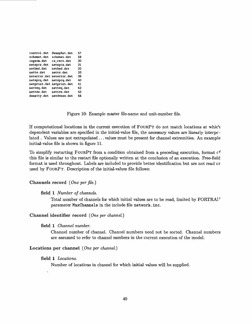
control . dat SwampRat . dats chemat . dat s chemat . datcxgeom . dat cx_rect . datnetspcz.dat netspcz.datnetbnd . dat netbnd . datnett s . dat nett s . datneterror.dat neterror.datnetspcq.dat netspcq.datnetprint . dat netprint . datnettsq.dat nettsq.datnettsz.dat nettsz.datdens ity . dat netdens e . dat
575830313233394041424344
Figure 10: Example master file-name and unit-number file.
If computational locations in the current execution of FOURPT do not match locations at which dependent variables are specified in the initial-value file, the necessary values are linearly interpo lated . Values are not extrapolated ... values must be present for channel extremities. An example initial-value file is shown in figure 11.
To simplify restarting FOURPT from a condition obtained from a preceding execution, format cf this file is similar to the restart file optionally written at the conclusion of an execution. Free-field format is used throughout. Labels are included to provide better identification but are not read or used by FOURPT. Description of the initial-values file follows:
Channels record (One per file.)
field 1 Number of channels.Total number of channels for which initial values are to be read, limited by FORTRA1 T parameter MaxChannels in the include file network.inc.
Channel identifier record (One per channel)
field 1 Channel number.Channel number of channel. Channel numbers need not be sorted. Channel numbers are assumed to refer to channel numbers in the current execution of the model.
Locations per channel (One per channel.)
field 1 Locations.Number of locations in channel for which initial values will be supplied.
40
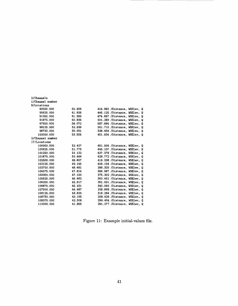
2/Channels 1 /Channel number8/Locations
90000,90625.91250.91875.97500.98125.98750.
100000,
,000,000000,000,000.000,000,000
62,61.61,60,56.55,55.55.
.456
.926
.385
.835,070.836.691.555
414.446.474.501,587.561.528.451,
,962.125,897.283.684.716.455,934
/Distance,/Distance,/Distance,/Distance,/Distance,/Distance,/Distance,/Distance,
WSElev,WSElev,WSElev,WSElev,WSElev,WSElev,WSElev,WSElev,
QQQQQQQQ
2/Channel number17 /Locations
100000,100625.101250,101875102500,103125103750,104375105000105625106250106875107500108125,108750109375110000
.000
.000
.000
.000
.000,000.000.000.000.000.000.000.000.000.000.000.000
52,515150494948474746,45,454443434241
.427
.776
.122
.466
.807
.145
.481
.816
.150,483.817.151.487.825.165.508.855
451.445437,428419409398386375363351340328318308299291
.934
.107
.378
.772
.338
.154
.325
.987
.302
.451
.631
.040
.868
.284
.428
.404
.277
/Distance,/Distance,/Distance,/Distance,/Distance,/Distance,/Distance,/Distance,/Distance,/Distance,/Distance,/Distance,/Distance,/Distance,/Distance,/Distance,/Distance,
WSElev,WSElev,WSElev,WSElev,WSElev,WSElev,WSElev,WSElev,WSElev,WSElev,WSElev,WSElev,WSElev,WSElev,WSElev,WSElev,WSElev,
QQQQQQQQQQQQQQQQQ
Figure 11: Example initial-values file.
41
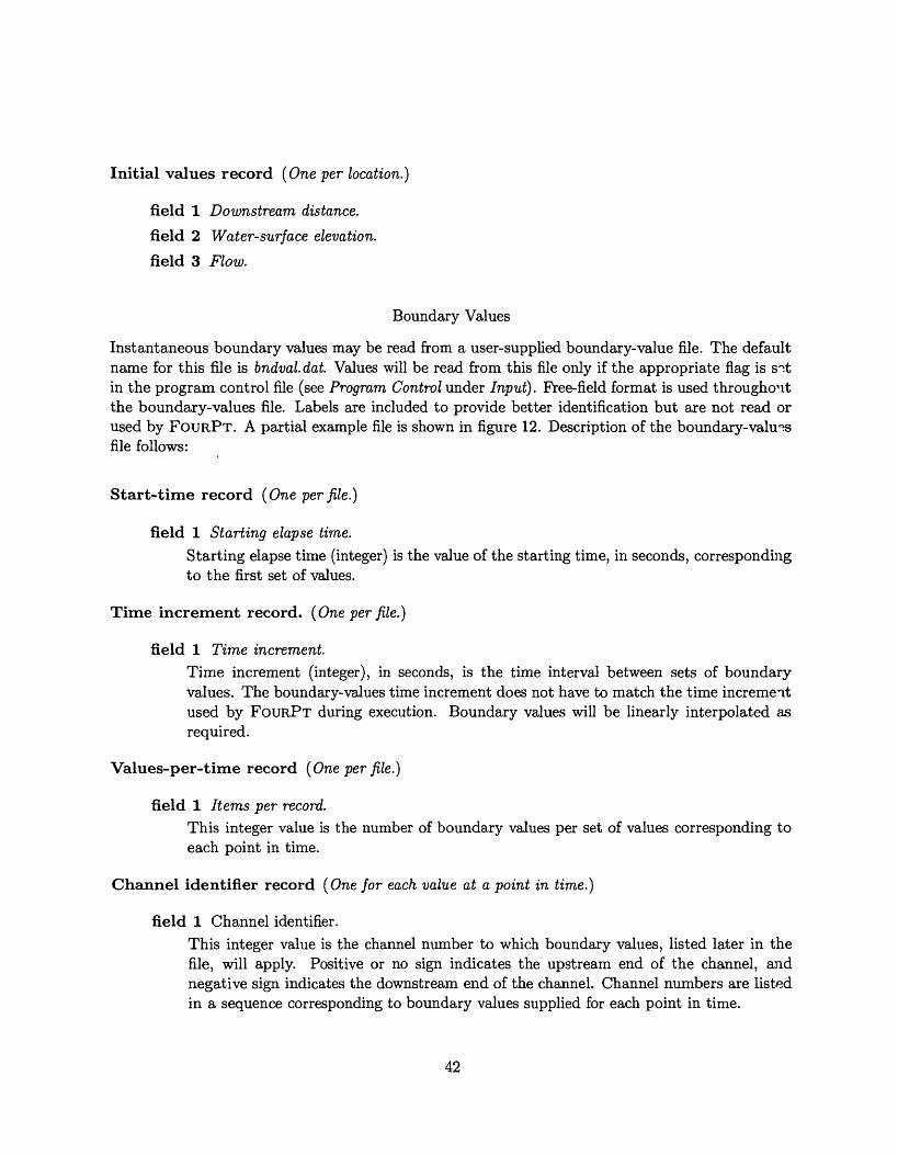
Initial values record (One per location.)
field 1 Downstream distance.
field 2 Water-surface elevation.
field 3 Flow.
Boundary Values
Instantaneous boundary values may be read from a user-supplied boundary-value file. The default name for this file is bndval. dat. Values will be read from this file only if the appropriate flag is snt in the program control file (see Program Control under Input). Free-field format is used throughont the boundary-values file. Labels are included to provide better identification but are not read or used by FouaPT. A partial example file is shown in figure 12. Description of the boundary-values file follows:
Start-time record (One per file.)
field 1 Starting elapse time.Starting elapse time (integer) is the value of the starting time, in seconds, corresponding to the first set of values.
Time increment record. (One per file.)
field 1 Time increment.Time increment (integer), in seconds, is the time interval between sets of boundary values. The boundary-values time increment does not have to match the time increment used by FouaPT during execution. Boundary values will be linearly interpolated as required.
Values-per-time record (One per file.)
field 1 Items per record.This integer value is the number of boundary values per set of values corresponding to each point in time.
Channel identifier record (One for each value at a point in time.)
field 1 Channel identifier.This integer value is the channel number to which boundary values, listed later in the file, will apply. Positive or no sign indicates the upstream end of the channel, and negative sign indicates the downstream end of the channel. Channel numbers are listed in a sequence corresponding to boundary values supplied for each point in time.
42
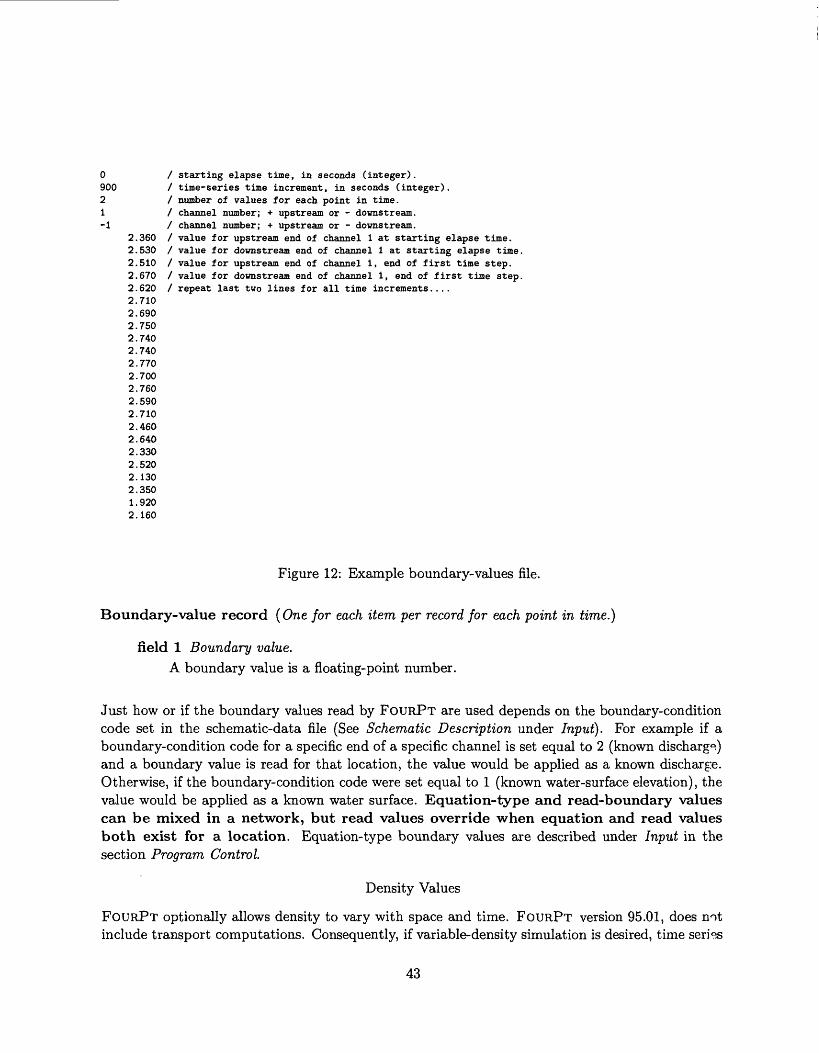
0 / starting elapse time, in seconds (integer).900 / time-series time increment, in seconds (integer).2 / number of values for each point in time.1 / channel number; + upstream or - downstream.-1 / channel number; + upstream or - downstream.
2.360 / value for upstream end of channel 1 at starting elapse time.2.530 / value for downstream end of channel 1 at starting elapse time.2.510 / value for upstream end of channel 1, end of first time step.2.670 / value for downstream end of channel 1, end of first time step.2.620 / repeat last two lines for all time increments....2.7102.6902.7502.7402.7402.7702.7002.7602.5902.7102.4602.6402.3302.5202.1302.3501.9202.160
Figure 12: Example boundary-values file.
Boundary-value record (One for each item per record for each point in time.}
field 1 Boundary value.A boundary value is a floating-point number.
Just how or if the boundary values read by FOURPT are used depends on the boundary-condition code set in the schematic-data file (See Schematic Description under Input}. For example if a boundary-condition code for a specific end of a specific channel is set equal to 2 (known discharge) and a boundary value is read for that location, the value would be applied as a known discharge. Otherwise, if the boundary-condition code were set equal to 1 (known water-surface elevation), the value would be applied as a known water surface. Equation-type and read-boundary values can be mixed in a network, but read values override when equation and read values both exist for a location. Equation-type boundary values are described under Input in the section Program Control.
Density Values
FouaPT optionally allows density to vary with space and time. FouaPT version 95.01, does not include transport computations. Consequently, if variable-density simulation is desired, time series
43
0900
0098001420009800142000990014800099001480010100151001020015400103001550010500155001070
starting elapse time, in seconds (integer), time-series time increment, in seconds (integer), value for upstream end of channel 1 at starting elapse time, value for downstream end of channel 1 at starting elapse time, value for upstream end of channel 2 at starting elapse time, value for downstream end of channel 2 at starting elapse time, value for upstream end of channel 1, end of first time step, value for downstream end of channel 1, end of first time step, value for upstream end of channel 2, end of first time step. value for downstream end of channel 2, end of first time step, repeat last four lines (2 per channel) for all time increments.
1.01560
Figure 13: Example density-values file for a two-channel network.
of instantaneous density values for the duration of a model run are input for both ends of each channel. Intervening density values are approximated by linear interpolation.
Instantaneous density values are read from a user-supplied density-value file. The default name for this file is density. dat. An example of such a file for a two-channel network is shown in figure 13.
Values will be read from this file only if the appropriate flag is set in the program control file (fee Program Control under Input). Free-field format is used throughout the density-values file. Labels are included to provide better identification but are not read or used by FoURPT. Description of the density-values file follows:
Start-time record (One per file.)
field 1 Starting elapse time.Starting elapse time (integer) is the value of the starting time, in seconds, corresponding to the first set of values.
Time increment record. (One per file.)
field 1 Time increment.Time increment (integer), in seconds, is the time interval between sets of density valuQ5. The density-values time increment does not have to match the time increment used by FouaPT during execution. Density values will be linearly interpolated as required.
44
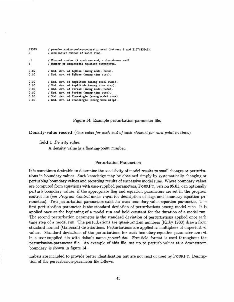
12345 / pseudo-random-number-generator seed (between 1 and 2147483646)0 / cumulative number of model runs.
-1 / Channel number (+ upstream end, - downstream end).1 / Number of sinusoidal equation components.
0.02 / Std. dev. of EqBase (among model runs).0.00 / Std. dev. of EqBase (among time step).
0.00 / Std. dev. of Amplitude (among model runs).0.00 / Std. dev. of Amplitude (among time step).0.00 / Std. dev. of Period (among model runs).0.00 / Std. dev. of Period (among time step).0.00 / Std. dev. of Phase Angle (among model runs).0.00 / Std. dev. of PhaseAngle (among time step).
Figure 14: Example perturbation-parameter file.
Density-value record (One value for each end of each channel for each point in time.}
field 1 Density value.A density value is a floating-point number.
Perturbation Parameters
It is sometimes desirable to determine the sensitivity of model results to small changes or perturta- tions in boundary values. Such knowledge may be obtained simply by systematically changing or perturbing boundary values and recording results of successive model runs. Where boundary values are computed from equations with user-supplied parameters, FOURPT, version 95.01, can optionally perturb boundary values, if the appropriate flag and equation parameters are set in the program control file (see Program Control under Input for description of flags and boundary-equation p a- rameters). Two perturbation parameters exist for each boundary-value equation parameter. Tv<? first perturbation parameter is the standard deviation of perturbations among model runs. It is applied once at the beginning of a model run and held constant for the duration of a model run. The second perturbation parameter is the standard deviation of perturbations applied once ea^,h time step of a model run. The perturbations are quasi-random numbers (Kirby 1983) drawn frcm standard normal (Gaussian) distributions. Perturbations are applied as multipliers of unperturb^ values. Standard deviations of the perturbations for each boundary-equation parameter are set in a user-supplied file with default name perturb.dat. Free-field format is used throughout the perturbation-parameter file. An example of this file, set up to perturb values at a downstreem boundary, is shown in figure 14.
Labels are included to provide better identification but are not read or used by FOURPT. Descrip tion of the perturbation-parameter file follows:
45
Seed record (One per file.}
field 1 Quasi-random number generator seed.The seed is an integer between 1 and 2147483646.
Counter record. ( One per file.}
field 1 Cumulative number of model runs.This integer value is increased by one each execution of the model when the perturbation feature is active. Thus, if initially set to zero, it will indicate the number of model runs executed in the current sequence of model runs.
Channel-identifier record (One per boundary perturbed.)
field 1 Channel number.
Integer specifies to which channel a perturbation refers. If positive, it relates to tl^ upstream end of the channel, and if negative, it refers to the downstream end of t\^ a. channel.
Equation components record. (One per boundary perturbed.)
field 1 Number of sinusoidal components.Integer is the number of sinusoidal components used in the current equation. This value must match the number of components entered in the program control file (see Program Control under Input).
First equation-base perturbation record (One per boundary perturbed.)
field 1 First standard deviation of equation base.Floating-point number is the standard deviation of the base value (about which sinu soidal components oscillate). This is the standard deviation of the distribution of values among model runs. The perturbation applied remains constant throughout a model run.
Second equation-base perturbation record (One per boundary perturbed.)
field 1 Second standard deviation of equation base.Floating-point number is the standard deviation of the base value (about which sinu soidal components oscillate). This is the standard deviation of the distribution of values within a model run. A different perturbation is applied each time step throughout a model run.
46
First amplitude perturbation record (One per sinusoidal component]
field 1 First standard deviation of amplitude.Floating-point number is the standard deviation of the amplitude of a sinusoidal com ponent. This is the standard deviation of the distribution of values among model runs. The perturbation applied remains constant throughout a model run.
Second amplitude perturbation record (One per sinusoidal component.}
field 1 Second standard deviation of amplitude.Floating-point number is the standard deviation of the amplitude of a sinusoidal com ponent. This is the standard deviation of the distribution of values within a model run. A different perturbation is applied each time step throughout a model run.
First period perturbation record (One per sinusoidal component.}
field 1 First standard deviation of period.Floating-point number is the standard deviation of the period of a sinusoidal component. This is the standard deviation of the distribution of values among model runs. Tv e perturbation applied remains constant throughout a model run.
Second period perturbation record (One per sinusoidal component.}
field 1 Second standard deviation of period.
Floating-point number is the standard deviation of the period of a sinusoidal component. This is the standard deviation of the distribution of values within a model run. A different perturbation is applied each time step throughout a model run.
First phase-angle perturbation record (One per sinusoidal component.}
field 1 First standard deviation of phase-angle.Floating-point number is the standard deviation of the phase-angle of a sinusoidal com ponent. This is the standard deviation of the distribution of values among model runs. The perturbation applied remains constant throughout a model run.
Second phase-angle perturbation record (One per sinusoidal component.}
field 1 Second standard deviation of phase-angle.Floating-point number is the standard deviation of the phase-angle of a sinusoidal com ponent. This is the standard deviation of the distribution of values within a model run. A different perturbation is applied each time step throughout a model run.
47
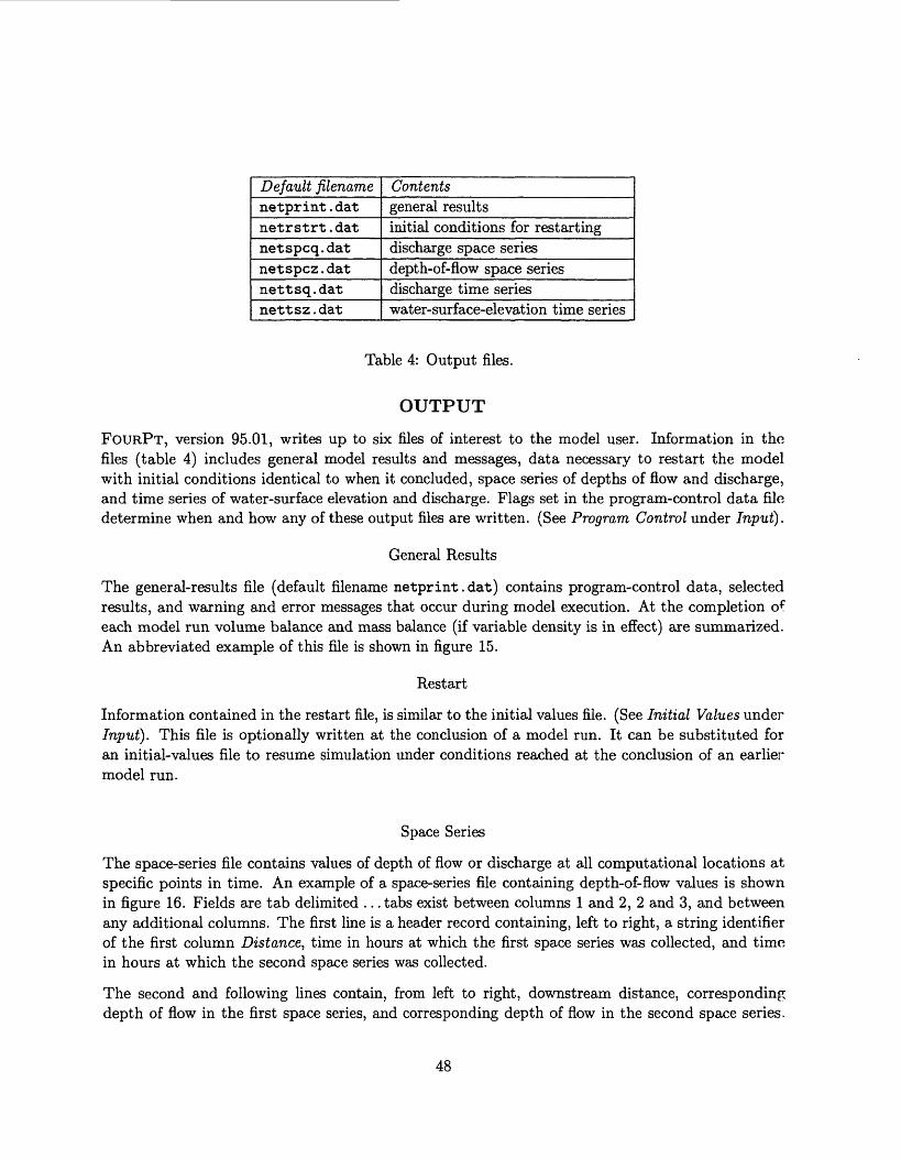
Default filenamenet print . datnetrstrt . datnetspcq.datnetspcz.datnettsq.datnettsz.dat
Contentsgeneral resultsinitial conditions for restartingdischarge space seriesdepth-of-flow space seriesdischarge time serieswater-surface-elevation time series
Table 4: Output files.
OUTPUT
FoURPx, version 95.01, writes up to six files of interest to the model user. Information in the files (table 4) includes general model results and messages, data necessary to restart the model with initial conditions identical to when it concluded, space series of depths of flow and discharge, and time series of water-surface elevation and discharge. Flags set in the program-control data file determine when and how any of these output files are written. (See Program Control under Input].
General Results
The general-results file (default filename netprint.dat) contains program-control data, selected results, and warning and error messages that occur during model execution. At the completion of each model run volume balance and mass balance (if variable density is in effect) are summarized. An abbreviated example of this file is shown in figure 15.
Restart
Information contained in the restart file, is similar to the initial values file. (See Initial Values under Input). This file is optionally written at the conclusion of a model run. It can be substituted for an initial-values file to resume simulation under conditions reached at the conclusion of an earlier model run.
Space Series
The space-series file contains values of depth of flow or discharge at all computational locations at specific points in time. An example of a space-series file containing depth-of-flow values is shown in figure 16. Fields are tab delimited ... tabs exist between columns 1 and 2, 2 and 3, and between any additional columns. The first line is a header record containing, left to right, a string identifier of the first column Distance, time in hours at which the first space series was collected, and time in hours at which the second space series was collected.
The second and following lines contain, from left to right, downstream distance, corresponding depth of flow in the first space series, and corresponding depth of flow in the second space series.
48
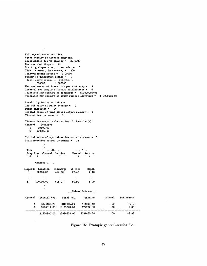
Full dynamic-wave solution... Water density is assumed constant. Acceleration due to gravity » 32.2000 Maximum time steps « 24 Starting elapse time, in seconds, - 0 Time increment, in seconds, « 300 Time-weighting factor « 1.00000 Number of quadrature points « 1 local coordinates..... weights...
.500000 1.000000Maximum number of iterations per time step ** 9 Interval for complete forward eliminations « 4 Tolerance for closure on discharge » 5.000000E-03 Tolerance for closure on water-surface elevation = 5.000000E-03
Level of printing activity « 1Initial value of print counter « 0Print increment - 24Initial value of time-series output counter = 0Time-series increment « 1
Time-series output selected for 2 Location(s): Channel Location
1 99500.002 100500.00
Initial value of spatial-series output counter - 0 Spatial-series output increment » 24
Time ....Q.... ....Z....Step Iter. Channel Section Channel Section24 3 1 17 21
Channel... 1
CompCxNo Location Discharge WSJElev Depth 1 90000.00 414.96 62.46 2.46
17 100000.00 506.97 56.99 6.99
__Volume Balance__
Channel Initial vol. Final vol. Junction Lateral Difference
1 3374468.20 3819365.00 444893.40 .00 3.132 8556511.00 10179270.00 1622762.00 .00 -6.00
11930980.00 13998632.00 2067655.30 .00 -2.88
Figure 15: Example general-results file.
49
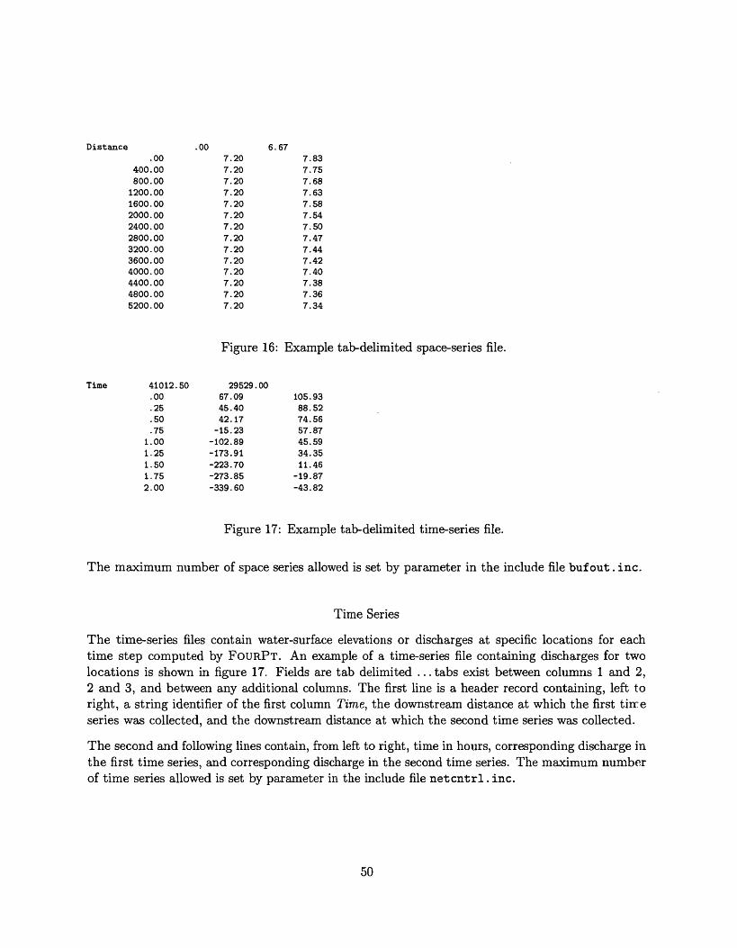
Distance .00 6.67.00
400.00800.001200.001600.002000.002400.002800.003200.003600.004000.004400.004800.005200.00
,20 ,20 ,20 .20 .20 .20 .20 ,20 .20 .20 .20 .20 .20
,83 .75 .68 .63 .58 .54 .50 .47 .44 .42 .40 .38 .36
7.20 7.34
Figure 16: Example tab-delimited space-series file.
Time 41012.50.00.25.50.75
1.001.251.501.752.00
29529.0067.0945.4042.17-15.23
-102.89-173.91-223.70-273.85-339.60
105.9388.5274.5657.8745.5934.3511.46
-19.87-43.82
Figure 17: Example tab-delimited time-series file.
The maximum number of space series allowed is set by parameter in the include file buf out. inc.
Time Series
The time-series files contain water-surface elevations or discharges at specific locations for each time step computed by FoURPT. An example of a time-series file containing discharges for two locations is shown in figure 17. Fields are tab delimited ... tabs exist between columns 1 and 2, 2 and 3, and between any additional columns. The first line is a header record containing, left to right, a string identifier of the first column Time, the downstream distance at which the first tirre series was collected, and the downstream distance at which the second time series was collected.
The second and following lines contain, from left to right, time in hours, corresponding discharge in the first time series, and corresponding discharge in the second time series. The maximum number of time series allowed is set by parameter in the include file netcntrl.inc.
50
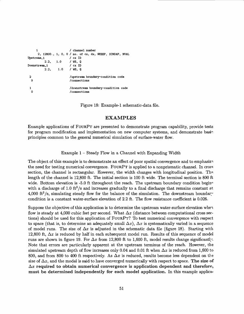
1 / channel number2, 12800., 1, 0, 0 / no. of ex, dx, NKEEP, ICNDAP, NVAL
Upstream.l / ex ID2.2, 1.0 / WS, Q
Downstream_l / ex ID2.2, 1.0 / WS, Q
2 /upstream boundary-condition code0 /connections
1 /downstream boundary-condition code0 /connections
Figure 18: Example-1 schematic-data file.
EXAMPLES
Example applications of FOURPT are presented to demonstrate program capability, provide tests for program modification and implementation on new computer systems, and demonstrate basin principles common to the general numerical simulation of surface-water flow.
Example 1 - Steady Flow in a Channel with Expanding Width
The object of this example is to demonstrate an effect of poor spatial convergence and to emphasize the need for testing numerical convergence. FOURPT is applied to a nonprismatic channel. In cross section, the channel is rectangular. However, the width changes with longitudinal position. Th^ length of the channel is 12,800 ft. The initial section is 100 ft wide. The terminal section is 800 ft wide. Bottom elevation is -5.0 ft throughout the reach. The upstream boundary condition begin*5 with a discharge of 1.0 ft3 /s and increases gradually to a final discharge that remains constant at 4,000 ft3 /s, simulating steady flow for the balance of the simulation. The downstream boundary condition is a constant water-surface elevation of 2.2 ft. The flow resistance coefficient is 0.026.
Suppose the objective of this application is to determine the upstream water-surface elevation when flow is steady at 4,000 cubic feet per second. What Ax (distance between computational cross sec tions) should be used for this application of FoURPT? To test numerical convergence with respect to space (that is, to determine an adequately small Ax), Ax is systematically varied in a sequence of model runs. The size of Ax is adjusted in the schematic data file (figure 18). Starting with 12,800 ft, Ax is reduced by half in each subsequent model run. Results of this sequence of model runs are shown in figure 19. For Ax from 12,800 ft to 1,600 ft, model results change significantly. Note that errors are particularly apparent at the upstream terminus of the reach. However, the simulated upstream depth of flow increases only 0.04 and 0.01 ft when Ax is reduced from 1,600 to 800, and from 800 to 400 ft respectively. As Ax is reduced, results become less dependent on the size of Ax, and the model is said to have converged numerically with respect to space. The size of Ax required to obtain numerical convergence is application dependent and therefore, must be determined independently for each model application. In this example applica-
51
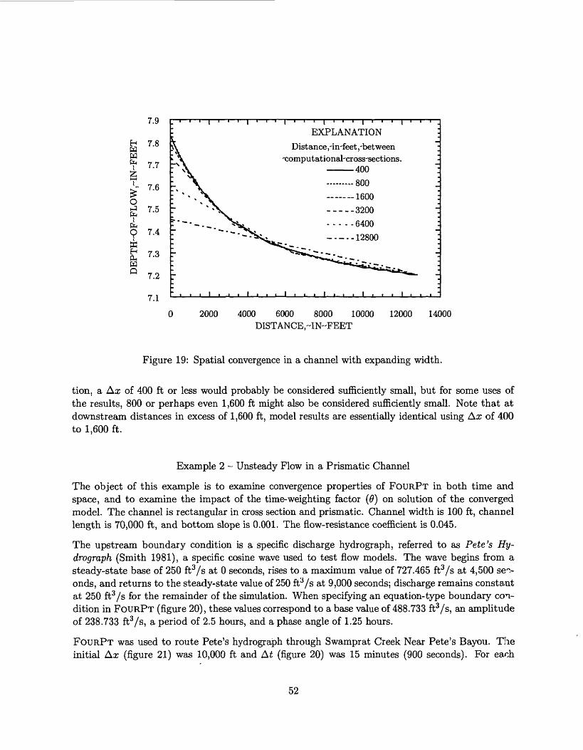
7.9
*? 7.7
- 7.6
7.5
9 7.4
ffi
7.2
7.1
EXPLANATIONDistance ,-in-feet ,-bet ween
-computational'cross-sections. 400
......... 800
.......1600
-----3200
6400
2000 4000 6000 8000 10000 DISTANCE,~IN"FEET
12000 14000
Figure 19: Spatial convergence in a channel with expanding width.
tion, a Ax of 400 ft or less would probably be considered sufficiently small, but for some uses of the results, 800 or perhaps even 1,600 ft might also be considered sufficiently small. Note that at downstream distances in excess of 1,600 ft, model results are essentially identical using Ax of 400 to 1,600 ft.
Example 2 - Unsteady Flow in a Prismatic Channel
The object of this example is to examine convergence properties of FOURPT in both time and space, and to examine the impact of the time-weighting factor (9} on solution of the converged model. The channel is rectangular in cross section and prismatic. Channel width is 100 ft, channel length is 70,000 ft, and bottom slope is 0.001. The flow-resistance coefficient is 0.045.
The upstream boundary condition is a specific discharge hydrograph, referred to as Pete's Hy- drograph (Smith 1981), a specific cosine wave used to test flow models. The wave begins from a steady-state base of 250 ft3 /s at 0 seconds, rises to a maximum value of 727.465 ft3 /s at 4,500 sec onds, and returns to the steady-state value of 250 ft3 /s at 9,000 seconds; discharge remains constant at 250 ft3 /s for the remainder of the simulation. When specifying an equation-type boundary con dition in FOURPT (figure 20), these values correspond to a base value of 488.733 ft3 /s, an amplitude of 238.733 ft3 /s, a period of 2.5 hours, and a phase angle of 1.25 hours.
FOURPT was used to route Pete's hydrograph through Swamprat Creek Near Pete's Bayou. The initial Ax (figure 21) was 10,000 ft and Ai (figure 20) was 15 minutes (900 seconds). For each
52
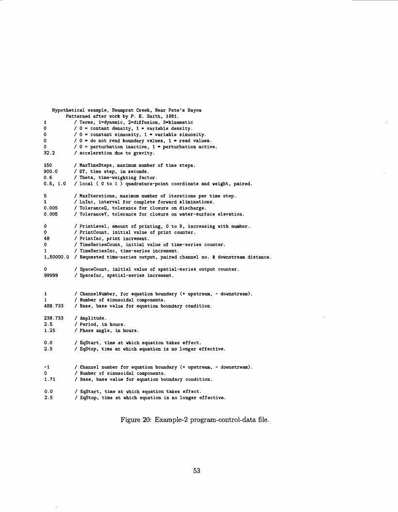
Hypothetical example, Swamprat Creek, Near Pete's BayouPatterned after work by P. E. Smith, 1981.
1 / Terms, l=dynamic, 2=diffusion, 3«kinematic0 / 0 = contant density, 1 - variable density.0 / 0 = constant sinuosity, 1 » variable sinuosity.0 / 0 = do not read boundary values, 1 » read values.0 / 0 = perturbation inactive, 1 » perturbation active.32.2 / acceleration due to gravity.
150 / MaxTimeSteps, maximum number of time steps.900.0 / DT, time step, in seconds.0.6 / Theta, time-weighting factor.0.5, 1.0 / local ( 0 to 1 ) quadrature-point coordinate and weight, paired.
5 / Maxlterations, maximum number of iterations per time step.1 / Lulnc, interval for complete forward eliminations.0.005 / ToleranceQ, tolerance for closure on discharge.0.005 / ToleranceY, tolerance for closure on water-surface elevation.
0 / PrintLevel, amount of printing, 0 to 9, increasing with number.0 / PrintCount, initial value of print counter.48 / Printlnc, print increment.0 / TimeSeriesCount, initial value of time-series counter.1 / TimeSeriesInc, time-series increment.1,50000.0 / Requested time-series output, paired channel no. ft downstream distance.
0 / SpaceCount, initial value of spatial-series output counter.99999 / Spacelnc, spatial-series increment.
1 / ChannelNumber, for equation boundary (+ upstream, - downstream).1 / Number of sinusoidal components.488.733 / Base, base value for equation boundary condition.
238.733 / Amplitude.2.5 / Period, in hours.1.25 / Phase angle, in hours.
0.0 / EqStart, time at which equation takes effect.2.5 / EqStop, time at which equation is no longer effective.
-1 / Channel number for equation boundary (+ upstream, - downstream)0 / Number of sinusoidal components.1.71 / Base, base value for equation boundary condition.
0.0 / EqStart, time at which equation takes effect.2.5 / EqStop, time at which equation is no longer effective.
Figure 20: Example-2 program-control-data file.
53
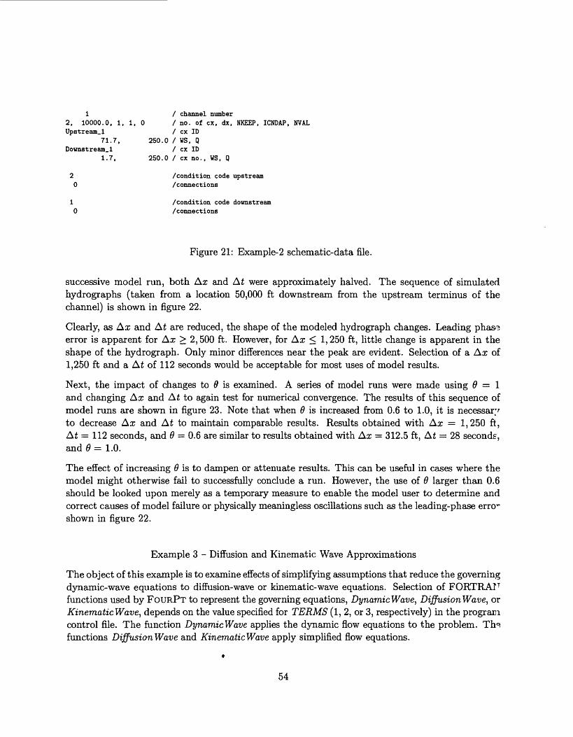
1 / channel number2, 10000.0, 1, 1, 0 / no. of ex, dx, NKEEP, ICNDAP, NVALUpstream.1 / ex ID
71.7, 250.0 / WS, QDownstream.! / ex ID
1.7, 250.0 / ex no., WS, Q
2 /condition code upstream0 /connections
1 /condition code downstream0 /connections
Figure 21: Example-2 schematic-data file.
successive model run, both Ax and At were approximately halved. The sequence of simulated hydrographs (taken from a location 50,000 ft downstream from the upstream terminus of the channel) is shown in figure 22.
Clearly, as Ax and At are reduced, the shape of the modeled hydrograph changes. Leading phas<? error is apparent for Ax > 2,500 ft. However, for Ax < 1,250 ft, little change is apparent in the shape of the hydrograph. Only minor differences near the peak are evident. Selection of a Ax of 1,250 ft and a At of 112 seconds would be acceptable for most uses of model results.
Next, the impact of changes to 9 is examined. A series of model runs were made using 0 = 1 and changing Ax and At to again test for numerical convergence. The results of this sequence of model runs are shown in figure 23. Note that when 0 is increased from 0.6 to 1.0, it is necessary to decrease Ax and At to maintain comparable results. Results obtained with Ax = 1,250 ft, At = 112 seconds, and 9 = 0.6 are similar to results obtained with Ax = 312.5 ft, At = 28 seconds, and 6 = 1.0.
The effect of increasing 0 is to dampen or attenuate results. This can be useful in cases where the model might otherwise fail to successfully conclude a run. However, the use of 0 larger than 0.6 should be looked upon merely as a temporary measure to enable the model user to determine and correct causes of model failure or physically meaningless oscillations such as the leading-phase erro^ shown in figure 22.
Example 3 - Diffusion and Kinematic Wave Approximations
The object of this example is to examine effects of simplifying assumptions that reduce the governing dynamic-wave equations to diffusion-wave or kinematic-wave equations. Selection of FORTRAN functions used by FouRPT to represent the governing equations, Dynamic Wave, DiffusionWave, or Kinematic Wave, depends on the value specified for TERMS (1, 2, or 3, respectively) in the program control file. The function DynamicWave applies the dynamic flow equations to the problem. Th^ functions DiffusionWave and KinematicWave apply simplified flow equations.
54
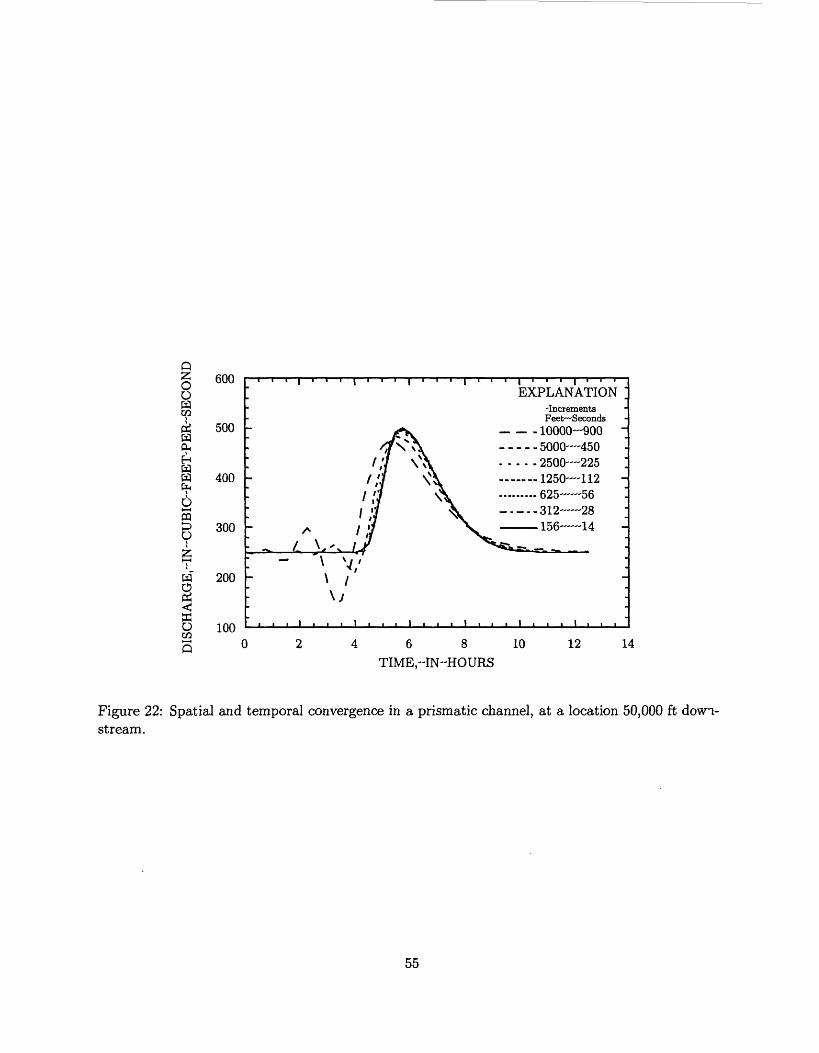
O OHCO
a
H
65D O
2 H-i
H
oCO
600
500 -
400 -
300 -
200 -
100
EXPLANATION-Increments Feet Seconds
- -10000 900- - - 5000 450- - . 2500 225- 1250 112 ..... 625 56---312 28
156 14
6 8 TIME,--IN~HOURS
10 12 14
Figure 22: Spatial and temporal convergence in a prismatic channel, at a location stream.
50,000 ft dovn-
55
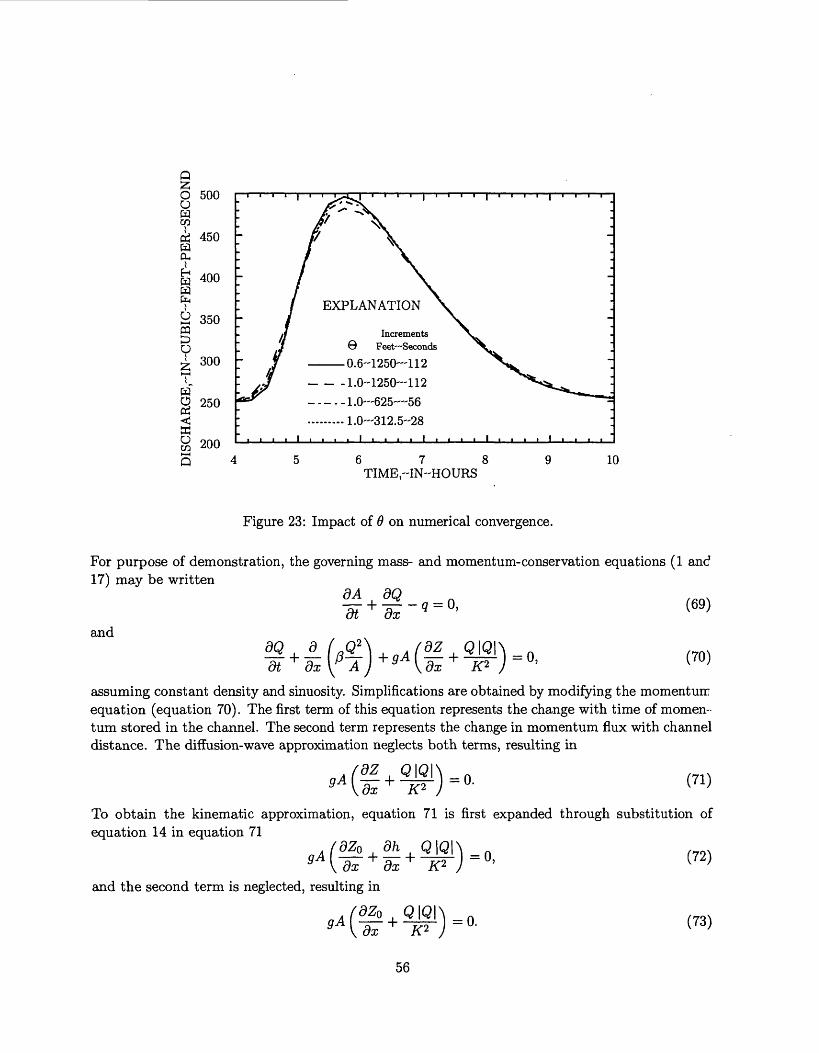
Q
O 500uH c
HPH
a
O
ffi
450
400
350PQ
300
250
200
Increments 0 Feet Seconds
0.6"1250~'112 1.0-1250 112 1.0 625 -56
1.0-312.5-28
678 TIME,'-IN-HOURS
10
Figure 23: Impact of 9 on numerical convergence.
For purpose of demonstration, the governing mass- and momentum-conservation equations (1 anc1 17) may be written
and
(70)
assuming constant density and sinuosity. Simplifications are obtained by modifying the momentum equation (equation 70). The first term of this equation represents the change with time of momen tum stored in the channel. The second term represents the change in momentum flux with channel distance. The diffusion-wave approximation neglects both terms, resulting in
' 9Z ^)=0. (71)
To obtain the kinematic approximation, equation 71 is first expanded through substitution ofequation 14 in equation 71
/ K7.n Ah n\n\\(72)
dx dx and the second term is neglected, resulting in
)
Q\Q\ (73)
56
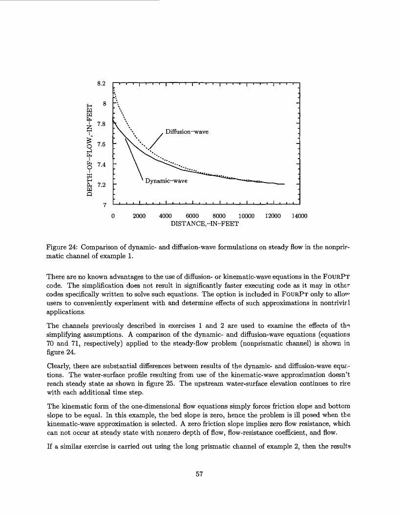
8.2
H
I T.8
7.6
§ 7.4
K
£ 7.2W Q
Diffusion wave
Dynamic-wave
0 2000 4000 6000 8000 10000 12000 14000 DISTANCE,-IN-FEET
Figure 24: Comparison of dynamic- and diffusion-wave formulations on steady flow in the nonprir- matic channel of example 1.
There are no known advantages to the use of diffusion- or kinematic-wave equations in the FOURPT code. The simplification does not result in significantly faster executing code as it may in other codes specifically written to solve such equations. The option is included in FOURPT only to allow users to conveniently experiment with and determine effects of such approximations in nontrivirl applications.
The channels previously described in exercises 1 and 2 are used to examine the effects of th^ simplifying assumptions. A comparison of the dynamic- and diffusion-wave equations (equations 70 and 71, respectively) applied to the steady-flow problem (nonprismatic channel) is shown in figure 24.
Clearly, there are substantial differences between results of the dynamic- and diffusion-wave equr- tions. The water-surface profile resulting from use of the kinematic-wave approximation doesn't reach steady state as shown in figure 25. The upstream water-surface elevation continues to rise with each additional time step.
The kinematic form of the one-dimensional flow equations simply forces friction slope and bottom slope to be equal. In this example, the bed slope is zero, hence the problem is ill posed when the kinematic-wave approximation is selected. A zero friction slope implies zero flow resistance, which can not occur at steady state with nonzero depth of flow, flow-resistance coefficient, and flow.
If a similar exercise is carried out using the long prismatic channel of example 2, then the results
57
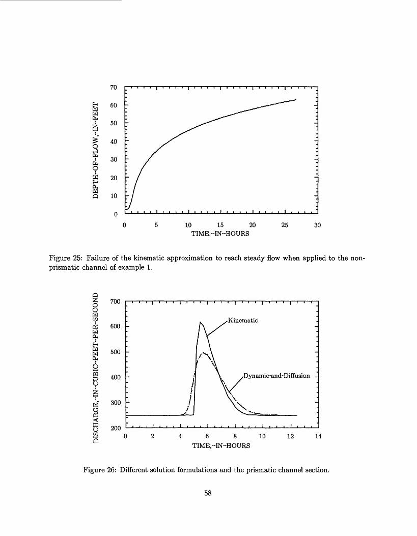
fa &
o.J fafa 9aE-i ou wQ
70
60
50
40
30
20
10
0
10 15 20 TIME,"IN-HOURS
25 30
Figure 25: Failure of the kinematic approximation to reach steady flow when applied to the non- prismatic channel of example 1.
O Owc
HOH
Ha w fa6HH
PQ ^o £HH
H
ffi oCOH I
Q
700
600
500
400
300
200
Kinematic
Dynamic-and-Diffusion -
4 6 8 10
TIME,~IN~HOURS12 14
Figure 26: Different solution formulations and the prismatic channel section.
58

Channel number and positive-flow direction
Figure 27: Schematic representation of a simple six-channel network.
shown in figure 26 are generated. For this channel, the dynamic and diffusion forms of the one- dimensional flow equations yield nearly the same results. However, the kinematic approximation yields a hydrograph with a significantly greater and sharper peak than the other forms of the equa tions. Clearly, the kinematic approximation is inappropriate for this particular problem. In fact, a 9 of one was required to reach a solution for this problem.
Example 4 - Unsteady Flow in a Simple Network of Channels
The object of this example is to demonstrate flow simulation in a small (six-channel) network (figure 27). Input files for this example can be used as a guide for construction of more complex networks. This example is derived from work by Jobson and Schoellhamer (Jobson and Schoellhamer 1992).
FouaPT was operated and time series output were taken from channel 3, distance 41,012 ft and channel 4, distance 29,529 ft. These results are shown in figure 28. The example schematic-data file (figure 29) can be used as a template for creation of more complex channel networks. Note that each channel has both an upstream and a downstream boundary-condition code.
Example 5 - Applying User-Programmed Constraints
This example demonstrates the application of two of the three user-programmed constraints that have been provided with the source code as examples of user-programmed constraints (see section Constraint Properties under INPUT). Two channels, rectangular in cross section, are simulated. The upstream channel is 1,000-feet wide and 10,000-feet long with a bed slope of 0.01 and flow-
59
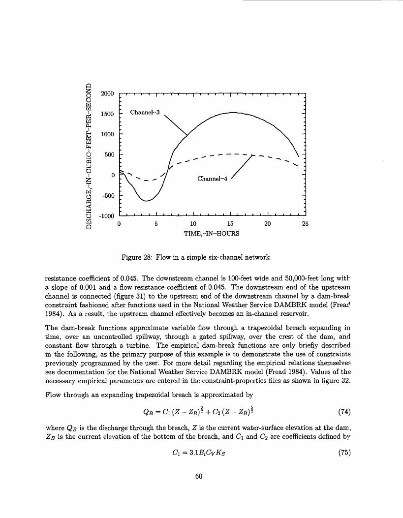
Q 55 O O WCO
WO,
W fa6HH
CQ £3 O
W
§<J ffl O en
2000
1500
1000
500
0
-500
-100010 15
TIME,"IN"HOURS
20 25
Figure 28: Flow in a simple six-channel network.
resistance coefficient of 0.045. The downstream channel is 100-feet wide and 50,000-feet long with a slope of 0.001 and a flow-resistance coefficient of 0.045. The downstream end of the upstream channel is connected (figure 31) to the upstream end of the downstream channel by a dam-breal- constraint fashioned after functions used in the National Weather Service DAMBRK model (Freac* 1984). As a result, the upstream channel effectively becomes an in-channel reservoir.
The dam-break functions approximate variable flow through a trapezoidal breach expanding in time, over an uncontrolled spillway, through a gated spillway, over the crest of the dam, and constant flow through a turbine. The empirical dam-break functions are only briefly described in the following, as the primary purpose of this example is to demonstrate the use of constraints previously programmed by the user. For more detail regarding the empirical relations themselves see documentation for the National Weather Service DAMBRK model (Fread 1984). Values of the necessary empirical parameters are entered in the constraint-properties files as shown in figure 32.
Flow through an expanding trapezoidal breach is approximated by
QB (74)
where QB is the discharge through the breach, Z is the current water-surface elevation at the dam, ZB is the current elevation of the bottom of the breach, and C\ and C? are coefficients defined by
(75)
60
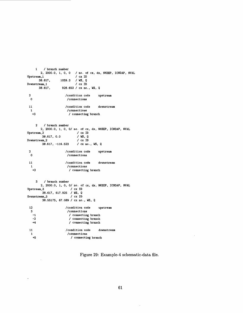
1 / branch number2, 2000.0, 1, 0, 0 / no. of ex, dx, NKEEP, ICNDAP, NVAL
Upstream.1 / ex ID38.617, 1059.3 / WS, Q
Downstream.1 / ex ID38.617, 928.653 / ex no., WS, Q
2 /condition code upstream0 /connections
11 /condition code downstream1 /connections+3 / connecting branch
2 / branch number2, 2000.0, 1, 0, O/ no. of ex, dx, NKEEP, ICNDAP, NVAL
Upstream_2 / ex ID 38.617, 0.0 / WS, Q
Downstream_2 / ex ID38.617, -116.523 / ex no., WS, Q
2 /condition code upstream 0 /connections
11 /condition code downstream1 /connections+3 / connecting branch
3 / branch number2, 2000.0, 1, 0, O/ no. of ex, dx, NKEEP, ICNDAP, NVAL
Upstream.3 / ex ID 38.617, 617.925 / WS, Q
Downstream_3 / ex ID38.55175, 67.089 / ex no., WS, Q
12 /condition code upstream3 /connections-1 / connecting branch-2 / connecting branch+4 / connecting branch
11 /condition code downstream1 /connections+5 / connecting branch
Figure 29: Example-4 schematic-data file.
61
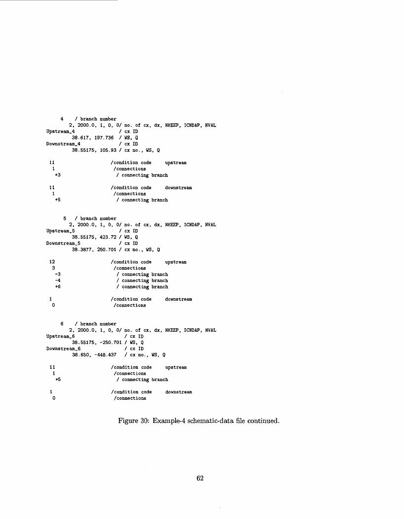
4 / branch number2, 2000.0, 1, 0, O/ no. of ex, dx, NKEEP, ICNDAP, NVAL
Upstream_4 / ex ID 38.617, 197.736 / WS, Q
Downstream_4 / ex ID38.55175, 105.93 / ex no., WS, Q
11 /condition code upstream1 /connections+3 I connecting branch
11 /condition code downstream1 /connections+5 / connecting branch
5 / branch number2, 2000.0, 1, 0, O/ no. of ex, dx, NKEEP, ICNDAP, NVAL
Upstream_5 / ex ID38.55175, 423.72 / WS, Q
Downstream_5 / ex ID38.3877, 250.701 / ex no., WS, Q
12 /condition code upstream3 /connections-3 / connecting branch-4 / connecting branch+6 / connecting branch
1 /condition code downstream0 /connections
6 / branch number2, 2000.0, 1, 0, O/ no. of ex, dx, NKEEP, ICNDAP, NVAL
Upstream_6 / ex ID 38.55175, -250.701 / WS, Q
Downstream_6 / ex ID38.650, -448.437 / ex no., WS, Q
11 /condition code upstream1 /connections+5 / connecting branch
1 /condition code downstream 0 /connections
Figure 30: Example-4 schematic-data file continued.
62
andC2 = ZMIssCvKs. (76)
Here BI is the current breach bottom width, Iss is inverse side slope of the breach, Cy is the velocity-correction coefficient defined by
r - 1 n i °-023Q2 Cv - W+
where Q is the total outflow from the reservoir, ZBM is the final breach bottom elevation, and is the width of the reservoir at the dam. KS in equations 75 and 76 is a submergence-correction coefficient defined by
#5 = 1.0, for Z ~ B <0.67 (78)
or 3
= 1.0- 27.8 - 0.67 , for - > 0.67, (79)\ 6 AB J 6 &B
where Z? is the tailwater elevation.
Flow over an uncontrolled spillway is approximated by
, (8o)
where Qs is flow over the spillway, Cs is the spillway coefficient, LS is the spillway width, and Zs is the spillway crest elevation.
Flow over the dam crest is approximated by
(81)
where QD is flow over the crest of the dam, CD is an empirical coefficient, LD is the width of the dam less the width of the uncontrolled spillway, and Zp is the dam-crest elevation.
Flow through a gated spillway is approximated by
= CGLG (Z-ZG ) l>, (82)
where QG is flow through the gate, CG is an empirical coefficient, LG is the gate flow area, and ZG is the center-line elevation of the gated spillway. The gated spillway function is not active in thb example; as shown in figure 32, the gated-spillway coefficient is zero.
Total discharge at the dam is the sum of the component discharges
Q = Qb + Qs + QD + QG . (83)
A second user-programmed constraint, a logarithmic relation between water-surface elevation and discharge, is applied as the boundary condition at the downstream end of the downstream channel. This relation takes the form
Z = Z0 + aQ\ (84)
63
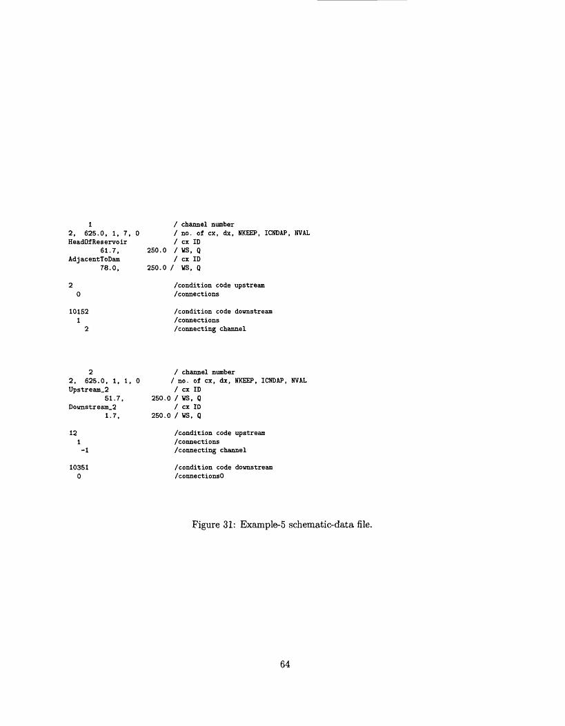
12, 625.0. 1, 7, HeadOfReservoir
61.7, AdjacentToDam
78.0,
/ channel number/no. of ex, dx, NKEEP, ICNDAP, NVAL/ ex ID
250.0 / MS, Q/ ex ID
250.0 / WS, Q
/condition code upstream /connections
101521
2
/condition code downstream /connections /connecting channel
22, 625.0, 1, Upstream_2
51.7, Downstream_2
1.7,
12 1 -1
103510
/ channel number 1,0 / no. of ex, dx, NKEEP, ICNDAP, NVAL
/ ex ID 250.0 / WS, Q
/ ex ID 250.0 / WS, Q
/condition code upstream /connections /connecting channel
/condition code downstream /connectionsO
Figure 31: Example-5 schematic-data file.
64
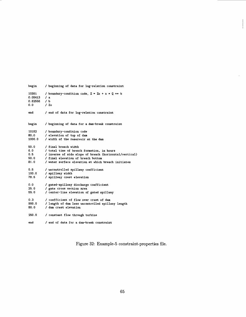
begin / beginning of data for log-relation constraint
10351 / boundary-condition code, Z-Zo+a*Q**b0.05413 / a0.62556 / b0.0 / Zo
end / end of data for log-relation constraint
begin / beginning of data for a dam-break constraint
10152 / boundary-condition code80.0 / elevation of top of dam1000.0 / width of the reservoir at the dam
50.0 / final breach width6.0 / total time of breach formation, in hours0.5 / inverse of side slope of breach (horizontal/vertical)50.0 / final elevation of breach bottom81.0 / water surface elevation at which breach initiates
0.5 / uncontrolled spillway coefficient100.0 / spillway width78.5 / spillway crest elevation
0.0 / gated-spillway discharge coefficient25.0 / gate cross section area55.0 / center-line elevation of gated spillway
0.3 / coefficient of flow over crest of dam900.0 / length of dam less uncontrolled spillway length80.0 / dam crest elevation
250.0 / constant flow through turbine
end / end of data for a dam-break constraint
Figure 32: Example-5 constraint-properties file.
65
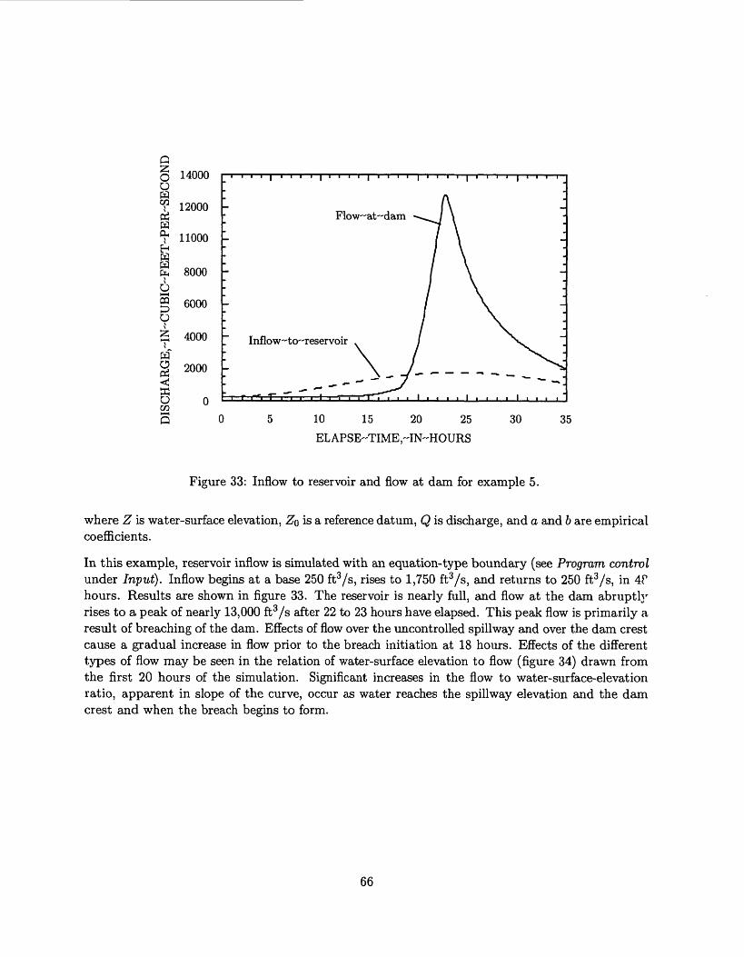
Qiz; OoH
1Ha,HHH fa
6so
T
1 rfffioCO
Q
14000
12000
11000
8000
6000
4000
2000
0
10 15 20 25
ELAPSE"TIME,~IN"HOURS
30 35
Figure 33: Inflow to reservoir and flow at dam for example 5.
where Z is water-surface elevation, ZQ is a reference datum, Q is discharge, and a and b are empirical coefficients.
In this example, reservoir inflow is simulated with an equation-type boundary (see Program control under Input). Inflow begins at a base 250 ft3 /s, rises to 1,750 ft3 /s, and returns to 250 ft3 /s, in 4P hours. Results are shown in figure 33. The reservoir is nearly full, and flow at the dam abruptly rises to a peak of nearly 13,000 ft3 /s after 22 to 23 hours have elapsed. This peak flow is primarily a result of breaching of the dam. Effects of flow over the uncontrolled spillway and over the dam crest cause a gradual increase in flow prior to the breach initiation at 18 hours. Effects of the different types of flow may be seen in the relation of water-surface elevation to flow (figure 34) drawn from the first 20 hours of the simulation. Significant increases in the flow to water-surface-elevation ratio, apparent in slope of the curve, occur as water reaches the spillway elevation and the dam crest and when the breach begins to form.
66
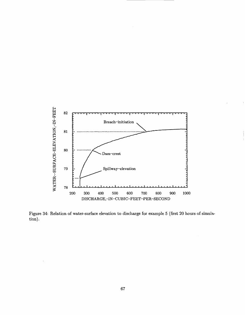
H 82
ao
O
£rt pCO
81
80
79
78
200 300 400 500 600 700 800 900 1000
DISCHARGE,~IN"CUBIC~FEET~PER~SECOND
Figure 34: Relation of water-surface elevation to discharge for example 5 (first 20 hours of simula tion) .
67
References
American National Standards Institute (1978). American National Standard Programming Lan guage FORTRAN. New York, N. Y.: American National Standards Institute.
Carnahan, B., H. A. Luther, and J. O. Wilkes (1969). Applied numerical methods. New York, New York: John Wiley and Sons, Inc.
Cunge, J. A., F. M. Holly. Jr., and A. Verwey (1980). Practical aspects of computational river hydraulics. Marshfield, MA: Pitman Publishing Inc.
DeLong, L. L. (1986). Extension of the unsteady one-dimensional open-channel flow equations for flow simulation in meandering channels with flood plains. In S. Subitzky (Ed.), Selected papers in the hydrol sci., pp. 101-105. U.S. Geolog. Water-Supply Paper 2290.
DeLong, L. L. (1989). Mass conservation: 1-d open channel flow equations. J. Hydr. Div., ASCE 115(2), 263-269.
DeLong, L. L. and J. M. Fulford (1993, JuL). General implicit representation of hydraulic struc tures in numerical flow models. In Proc. 1993 Nat. Conf. on Hydr. Engrg., pp. 1143-1148. ASCE.
DeLong, L. L. and D. H. Schoellhamer (1989). Computer program HYDRAUX - a model for sim ulating one-dimensional, unsteady, open-channel flow. U.S. Geolog. Survey Water Resources Investigations Report 88-4226.
DeLong, L. L., D. B. Thompson, and J. M. Fulford (1992). Data encapsulation using fortran 77 modules. Fortran Forum Jf^(3), 11-19.
Flanders, H., R. R. Korfhage, and J. J. Price (1974). A Second Course in Calculus. New York, NY: Academic Press.
Fread, D. L. (1984). DAMBRK: The NWS dam break forecasting model Silver Spring, Md.: Ofc. of Hydrol., National Weather Service.
Froehlich, D. C. (1990, Jul.). Hermite-Galerkin model for dam-break floods. In Proc. 1990 Nat. Conf. on Hydr. Engrg., pp. 557-562. ASCE.
Fulford, J. M. (1993). User's guide to hydraulic information exchange program: A computer program for hydraulic properties computations. On file with U.S. Geolog. Survey, at Stennis Space Center, MS 39529.
Jobson, H. E. and D. H. Schoellhamer (1992). User's manual for a branched Lagrangian transport model. U.S. Geolog. Survey Water Resources Investigations Report 87-4163.
Kirby, W. H. (1983). Computer routines for probability distributions, random numbers, and re lated functions. U.S. Geolog. Survey Water Resources Investigations Report 83-4257.
Preissmann, A. (1961, Sep.). Propagation des intumescences dans les canaux et rivieres. In 1st Congress de I' Assoc Francaise de Calcul, Grenoble, pp. 433-42.
Smith, P. E. (1981). Numerical experiments on three unsteady flow models. On file with U.S. Geolog. Survey, at Stennis Space Center, MS 39529.
68
Stroustrup, B. (1988, May). What is object-oriented programming? Software Magazine, IEEE, 10-20.
Thompson, D. B., L. L. DeLong, and J. M. Fulford (1992). Data Encapsulation Using Fortran-77 Modules a First Step Toward Object-Oriented Programming. U.S. Geolog. Survey Wate~ Resources Investigations Report 92-4123.
69


![F.95.01.T B - zentrum.virtuos.uni-osnabrueck.de · 1 F.95.01.T 1 zid B hinzufüg:IPT.SM (Red ) weiter! (B fragt einen Arbeiter [A] nach der Arbeit eines anderen, der daneben an einer](https://img.pdfslide.net/doc/110x75/5e02faa6d9e2ea2f2041304b/f9501t-b-1-f9501t-1-zid-b-hinzufgiptsm-red-weiter-b-fragt-einen.jpg)