The connection between Labrador Sea buoyancy loss, deep

Ocean Modelling 30 (2009) 207–224

Contents lists available at ScienceDirect

Ocean Modelling

journal homepage: www.elsevier .com/locate /ocemod

The connection between Labrador Sea buoyancy loss, deep western boundarycurrent strength, and Gulf Stream path in an ocean circulation model

Stephen G. Yeager *, Markus JochumNational Center for Atmospheric Research, Boulder, CO, USA

a r t i c l e i n f o a b s t r a c t

Article history:Received 30 October 2008Received in revised form 24 June 2009Accepted 29 June 2009Available online 10 July 2009

Keywords:Gulf StreamDeep western boundary currentMixed thermohaline boundary conditionsWater mass transformationNorth Atlantic

1463-5003/$ - see front matter � 2009 Elsevier Ltd. Adoi:10.1016/j.ocemod.2009.06.014

* Corresponding author. Address: Climate andNational Center for Atmospheric Research, Boulder, C303 497 17 21.

E-mail address: [email protected] (S.G. Yeager).

The sensitivity of the North Atlantic gyre circulation to high latitude buoyancy forcing is explored in aglobal, non-eddy resolving ocean general circulation model. Increased buoyancy forcing strengthensthe deep western boundary current, the northern recirculation gyre, and the North Atlantic Current,which leads to a more realistic Gulf Stream path. High latitude density fluxes and surface water masstransformation are strongly dependent on the choice of sea ice and salinity restoring boundary condi-tions. Coupling the ocean model to a prognostic sea ice model results in much greater buoyancy lossin the Labrador Sea compared to simulations in which the ocean is forced by prescribed sea ice boundaryconditions. A comparison of bulk flux forced hindcast simulations which differ only in their sea ice andsalinity restoring forcings reveals the effects of a mixed thermohaline boundary condition transport feed-back whereby small, positive temperature and salinity anomalies in subpolar regions are amplified whenthe gyre spins up as a result of increased buoyancy loss and convection. The primary buoyancy fluxeffects of the sea ice which cause the simulations to diverge are ice melt, which is less physical in thediagnostic sea ice model, and insulation of the ocean, which is less physical with the prognostic seaice model. Increased salinity restoring ensures a more realistic net winter buoyancy loss in the LabradorSea, but it is found that improvements in the Gulf Stream simulation can only be achieved with the exces-sive buoyancy loss associated with weak salinity restoring.

� 2009 Elsevier Ltd. All rights reserved.

1. Introduction

Simulations of the North Atlantic in non-eddy resolving oceangeneral circulation models (OGCMs) have historically suffered frompoor representation of the strength and path of the Gulf Stream(Dengg et al., 1996). The resulting large biases in the high-latitudetemperature and salinity fields seriously undermine the utility ofthese models for investigating oceanic and coupled climate pro-cesses in the North Atlantic. For instance, negative sea surface tem-perature (SST) biases east of the Grand Banks exceed 9 �C in onewidely used coupled climate model (Large and Danabasoglu, 2006).

Numerous studies have demonstrated that a marked improve-ment in the realism of the modeled North Atlantic circulation isobtainable at so-called eddy-resolving resolutions (horizontal res-olution 0.1�) in which the first mode baroclinic Rossby radius is re-solved and the mesoscale energy spectrum approaches observedlevels (e.g., Bryan et al., 2007; Smith et al., 2000; Hurlburt and Ho-gan, 2000; Oschlies, 2002; Brachet et al., 2004). However, the com-

ll rights reserved.

Global Dynamics Division,O 80307-3000, USA. Tel.: +1

putational expense of such high horizontal resolution precludesthe use of eddy-resolving models for long simulations or as theocean component in coupled climate models.

A remedy for the Gulf Stream (GS) problem for non-eddy resolv-ing (coarse) resolutions has been elusive, but important sensitivitieshave been identified. A stronger deep western boundary current(DWBC) pushes the latitude of the GS separation point to the south(Tansley and Marshall, 2000; Thompson and Schmitz, 1989; Ezerand Mellor, 1992; Dai et al., 2005). The DWBC is coupled to the GSthrough entrainment of upper DWBC water under the GS at thecrossover point (Spall, 1996), and bottom-vortex stretching inducedby a strong downslope DWBC south of the Grand Banks enhancesthe strengths of the northern recirculation gyre (NRG) and the NorthAtlantic Current (NAC) (Zhang and Vallis, 2007, hereafter referred toas ZV07). Since the DWBC is related to the strength of deep convec-tion and thermohaline forcing at high latitudes, perturbing the sur-face density in deep-water formation regions can have pronouncedeffects on GS circulation (Gerdes and Koberle, 1995).

Coarse resolution OGCMs are by necessity too viscous, becausethey must satisfy numerical constraints associated with the largegrid spacing (Large et al., 2001). However, a significantly improvedLabrador current and sea ice distribution can be obtained by lower-ing horizontal viscosity at the expense of increased grid-scale noise

http://dx.doi.org/10.1016/j.ocemod.2009.06.014

mailto:[email protected]

http://www.sciencedirect.com/science/journal/14635003

http://www.elsevier.com/locate/ocemod

208 S.G. Yeager, M. Jochum / Ocean Modelling 30 (2009) 207–224

(Jochum et al., 2008). Less momentum diffusion has been linked to astrengthening of the subpolar and northern recirculation gyres, andimproved GS separation in 1� OGCMs (ZV07; Doney et al., 2003).

Several studies have demonstrated that the GS system is sensi-tive to the details of how sub-gridscale mixing is parameterized.Danabasoglu et al. (2008) find that deep convection in the Labra-dor, Greenland, Irminger, and Norwegian Seas is considerably en-hanced with a parameterization for near surface mesoscale eddyfluxes (Ferrari et al., 2008). Allowing spatial and temporal varia-tions in the thickness diffusivity (Gent and McWilliams, 1990) gen-erates deeper Labrador Sea convection and reduces the negativetemperature biases east of the Grand Banks (Eden et al., 2009).When physically-based latitudinal structure is added to the back-ground vertical diffusivity such that diapycnal mixing is enhancedin the subtropics, deep convection is more robust, the DWBCstrengthens, and the GS shifts southward (Jochum, 2008).

The origins of systematic errors in OGCMs are generally ex-plored in uncoupled configurations in which the ocean surfaceboundary conditions are strongly constrained by observations.While this approach can generate quite realistic ocean simulationsin the Tropics, the North Atlantic is a particularly challenging re-gion to model because of the importance of sea-ice thermodynam-ics, buoyancy flux and bottom pressure torque. In the presentwork, we investigate the sensitivity of the North Atlantic circula-tion in a coarse resolution OGCM to surface forcing. We focus onthe model response to different forcing choices which are com-monplace in ocean model development, an activity which placesa premium on the realism of the ocean boundary conditions. Theeffects of the following are compared in configurations which useprescribed atmospheric forcing: (1) use of a prognostic versus adiagnostic sea ice model, (2) the use of interannual versus repeat-ing annual atmospheric conditions, and (3) the strength of surfacesalinity restoring. Configurations which maximize DWBC transportshow dramatic and unprecedented improvement in NAC strengthand GS path for the 1� version of the ocean component of CCSM;however, this is achieved only when the surface water mass forma-tion of Atlantic deep water exceeds reasonable rates. Excessive sur-

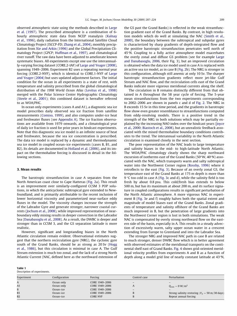
Fig. 1. Ocean bathymetry (km) from the POP 1� model

face transformation is shown to be an artifact of the circulationfeedbacks arising from mixed thermohaline boundary conditions.

2. Description of the model and experiments

The ocean and sea ice models used for all experiments aredevelopment versions of the component models of the CommunityClimate System Model (CCSM). The suite of models corresponds toCCSM 3.5, which is an interim version preceding the future releaseof CCSM 4. The ocean model is a z-coordinate, primitive equationglobal ocean model based on the Parallel Ocean Program (POP)developed at the Los Alamos National Laboratory (Smith et al.,1992; Dukowicz and Smith, 1994). The curvilinear horizontal meshis nominally 1� with 320 zonal and 384 meridional grid points andhas its northern grid pole displaced into Greenland. The oceanmodel differs from the CCSM 3 version described at length in Dana-basoglu et al. (2006) as follows:

� The vertical grid resolution is increased from 40 to 60 levelswith a layer of constant cell thickness of 10 m extending to160 m depth.

� The Ferrari et al. (2008) near-surface eddy flux parameterizationis implemented (Danabasoglu et al., 2008) with stratification-dependent enhancement of the isopycnal thickness diffusivity(Danabasoglu and Marshall, 2007).

� The anisotropic horizontal viscosity is reduced by one to twoorders of magnitude (Jochum et al., 2008).

� A parameterization for tidally-driven vertical diffusivity isimplemented (Jayne, 2009).

The North Atlantic bathymetry of the model shown in Fig. 1 high-lights some of the geographic features salient to the simulation ofthe Atlantic circulation and gives a sense of the enhanced resolu-tion in the vicinity of Greenland associated with the convergingmeridional lines of the 1� POP grid.

In each experiment (see Table 1), surface fluxes are computedfrom bulk formulae using the prognostic ocean model SST and an

with geographical features mentioned in the text.

S.G. Yeager, M. Jochum / Ocean Modelling 30 (2009) 207–224 209

observed atmospheric state using the methods described in Largeet al. (1997). The prescribed atmosphere is a combination of 6-hourly atmospheric state data from NCEP reanalysis (Kalnayet al., 1996), daily radiation from the International Satellite CloudClimatology Project (ISCCP-FD; Zhang et al., 2004), monthly precip-itation from Xie and Arkin (1996) and the Global Precipitation Cli-matology Project (GPCP; Huffman et al., 1997), and climatologicalriver runoff. The raw data have been adjusted to ameliorate knownsystematic biases. All experiments except one use the interannual-ly-varying forcing dataset (CORE.2-IAF) of Large and Yeager (2008),spanning 1949–2006. Experiment B2 uses a repeating normal yearforcing (CORE.2-NYF), which is identical to CORE.1-NYF of Largeand Yeager (2004) but uses updated adjustment factors. The initialcondition for the ocean in all experiments is a state of rest, withtemperature and salinity prescribed from the global climatologicaldistribution of the 1998 World Ocean Atlas (Levitus et al., 1998)merged with the Polar Science Center Hydrographic Climatology(Steele et al., 2001); this combined dataset is hereafter referredto as WOA/PHC.

In ocean only experiments (cases A and A1), a diagnostic sea icemodel prescribes daily observed sea ice fraction from satellitemeasurements (Comiso, 1999), and also computes under-ice heatand freshwater fluxes (see Appendix A). The ice fraction observa-tions are available from 1979 onwards, and a climatological yearof daily ice fraction is used for prior years in hindcast experiments.Note that this diagnostic sea ice model is an infinite source of heatand freshwater, because the sea ice concentration is prescribed.The data ice model is replaced by a dynamic and thermodynamicsea ice model in coupled ocean–ice experiments (cases B, B1, andB2). Its details are documented in Holland et al. (2006), and its im-pact on the thermohaline forcing is discussed in detail in the fol-lowing sections.

3. Mean results

The barotropic streamfunction in case A separates from theNorth American coast close to Cape Hatteras (Fig. 2a). This resultis an improvement over similarly-configured CCSM 3 POP solu-tions, in which the anticyclonic subtropical gyre extended to New-foundland, and is primarily attributable to the recent inclusion oflower horizontal viscosity and parameterized near-surface eddyfluxes in the model. The viscosity changes increase the strengthof the Labrador Gyre and generate stronger, narrower coastal cur-rents (Jochum et al., 2008), while improved representation of near-boundary eddy mixing results in deeper convection in the LabradorSea (Danabasoglu et al., 2008). As a result, the DWBC is deeper andstronger than in CCSM 3, and the GS separation latitude is morerealistic.

However, significant and longstanding biases in the NorthAtlantic circulation remain evident. Observational estimates sug-gest that the northern recirculation gyre (NRG), the cyclonic gyresouth of the Grand Banks, should be as strong as 20 Sv (Hogget al., 1986), but this circulation is minimal in case A. The GulfStream extension is much too zonal, and the lack of a strong NorthAtlantic Current (NAC, defined here as the northward extension of

Table 1Description of experiments.

Experiment Configuration Forcing

A Ocean only CORE 1949–2006A1 Ocean only CORE 1949–2006B Ocean–ice CORE 1949–2006B1 Ocean–ice CORE 1949–2006B2 Ocean–ice CORE NYF

the GS past the Grand Banks) is reflected in the weak streamfunc-tion gradient east of the Grand Banks. By contrast, in high resolu-tion models which do well at simulating the NAC (Smith et al.,2000), the boundary between the subtropical and subpolar gyresis characterized by sharp gradients of depth-integrated flow andthe positive barotropic streamfunction penetrates well north of45�N. Coupling to a fully active atmosphere model exacerbatesthe overly zonal and diffuse GS problem (see for example Largeand Danabasoglu, 2006, their Fig. 3), but an improved circulationis obtained when the data ice model used in case A is replaced withan active sea ice model, as in case B (Fig. 2b). The NRG is stronger inthis configuration, although still anemic at only 10 Sv. The sharperbarotropic streamfunction gradients reflect more jet-like GulfStream and NAC flow, and the recirculation cells east of the GrandBanks indicate more vigorous meridional currents along the shelf.

The circulation in B remains distinctly different from that ob-tained in A throughout the 58 year cycle of forcing. The 5-yearmean streamfunctions from the two experiments correspondingto 2002–2006 are shown in panels c and d of Fig. 2. The NRG inB exceeds 15 Sv in this time period, and the gradients in barotropicflow show even greater resemblance to streamfunctions computedfrom eddy-resolving models. There is a positive trend in thestrength of the NRG in both solutions which may be partially ex-plained by the increasing NAO index over the hindcast years (Joyceet al., 2000; Biastoch et al., 2008), but an unrealistic feedback asso-ciated with the mixed thermohaline boundary conditions contrib-utes to the trend. The interannual variability in the North Atlanticcirculation is examined closely in the next section.

The poor representation of the NAC leads to large temperatureand salinity biases in the mid- to high-latitude North Atlantic.The WOA/PHC climatology clearly shows the sharp northwardexcursion of isotherms east of the Grand Banks (50�W, 40�N) asso-ciated with the NAC, which transports warm and salty subtropicalwater into the Northwest Corner region (Rossby, 1996) where itretroflects to the east (Fig. 3). Because of an overly zonal GS, thetemperature east of the Grand Banks at 175 m depth is more than9 �C too cold in case A (Fig. 3c and d), while the salinity field is toofresh by about 0.8 psu. This cold/fresh bias extends to below500 m, but has its maximum at about 200 m, and its surface signa-ture in coupled configurations results in significant perturbation ofthe North Atlantic atmosphere. A more vigorous NAC in experi-ment B (Fig. 3e and f) roughly halves both the spatial extent andmagnitude of model biases east of the Grand Banks. Zonal gradi-ents of temperature and salinity offshore of the Grand Banks aremuch improved in B, but the penetration of large gradients intothe Northwest Corner region is lost in both simulations. The weakNAC is compensated by overly strong northward flow on the east-ern side of the basin, especially in A. This results in a steady advec-tion of excessively warm, salty upper ocean water in a crescentextending from Europe to Greenland and into the Labrador Sea.

The stronger NRG and improved NAC path in case B are relatedto much stronger, denser DWBC flow which is in better agreementwith observed estimates of the meridional transports on the conti-nental shelf east of Grand Banks. Fig. 4 shows grid-oriented merid-ional velocity profiles from experiments A and B as a function ofdepth along a model grid line of nearly constant latitude at 43�N,

Control case Perturbation

– –A Qmin ¼ 0 W=m2

– –B Strong salinity restoring ðVp ¼ 50 m=30 daysÞB Repeat annual forcing

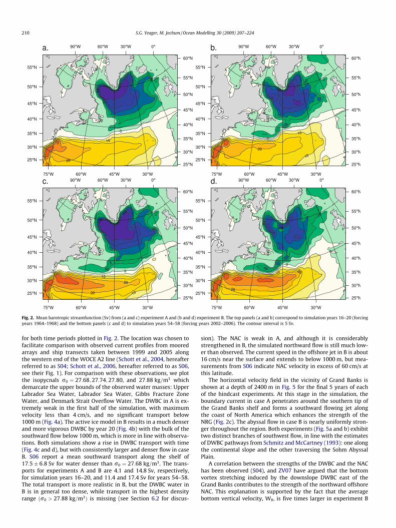
Fig. 2. Mean barotropic streamfunction (Sv) from (a and c) experiment A and (b and d) experiment B. The top panels (a and b) correspond to simulation years 16–20 (forcingyears 1964–1968) and the bottom panels (c and d) to simulation years 54–58 (forcing years 2002–2006). The contour interval is 5 Sv.


for both time periods plotted in Fig. 2. The location was chosen tofacilitate comparison with observed current profiles from mooredarrays and ship transects taken between 1999 and 2005 alongthe western end of the WOCE A2 line (Schott et al., 2004, hereafterreferred to as S04; Schott et al., 2006, hereafter referred to as S06,see their Fig. 1). For comparison with these observations, we plotthe isopycnals r0 ¼ 27:68;27:74;27:80, and 27:88 kg=m3 whichdemarcate the upper bounds of the observed water masses: UpperLabrador Sea Water, Labrador Sea Water, Gibbs Fracture ZoneWater, and Denmark Strait Overflow Water. The DWBC in A is ex-tremely weak in the first half of the simulation, with maximumvelocity less than 4 cm/s, and no significant transport below1000 m (Fig. 4a). The active ice model in B results in a much denserand more vigorous DWBC by year 20 (Fig. 4b) with the bulk of thesouthward flow below 1000 m, which is more in line with observa-tions. Both simulations show a rise in DWBC transport with time(Fig. 4c and d), but with consistently larger and denser flow in caseB. S06 report a mean southward transport along the shelf of17:5� 6:8 Sv for water denser than r0 ¼ 27:68 kg=m3. The trans-ports for experiments A and B are 4.1 and 14.8 Sv, respectively,for simulation years 16–20, and 11.4 and 17.4 Sv for years 54–58.The total transport is more realistic in B, but the DWBC water inB is in general too dense, while transport in the highest densityrange ðr0 > 27:88 kg=m3Þ is missing (see Section 6.2 for discus-

sion). The NAC is weak in A, and although it is considerablystrengthened in B, the simulated northward flow is still much low-er than observed. The current speed in the offshore jet in B is about16 cm/s near the surface and extends to below 1000 m, but mea-surements from S06 indicate NAC velocity in excess of 60 cm/s atthis latitude.

The horizontal velocity field in the vicinity of Grand Banks isshown at a depth of 2400 m in Fig. 5 for the final 5 years of eachof the hindcast experiments. At this stage in the simulation, theboundary current in case A penetrates around the southern tip ofthe Grand Banks shelf and forms a southward flowing jet alongthe coast of North America which enhances the strength of theNRG (Fig. 2c). The abyssal flow in case B is nearly uniformly stron-ger throughout the region. Both experiments (Fig. 5a and b) exhibittwo distinct branches of southwest flow, in line with the estimatesof DWBC pathways from Schmitz and McCartney (1993): one alongthe continental slope and the other traversing the Sohm AbyssalPlain.

A correlation between the strengths of the DWBC and the NAChas been observed (S04), and ZV07 have argued that the bottomvortex stretching induced by the downslope DWBC east of theGrand Banks contributes to the strength of the northward offshoreNAC. This explanation is supported by the fact that the averagebottom vertical velocity, WB, is five times larger in experiment B

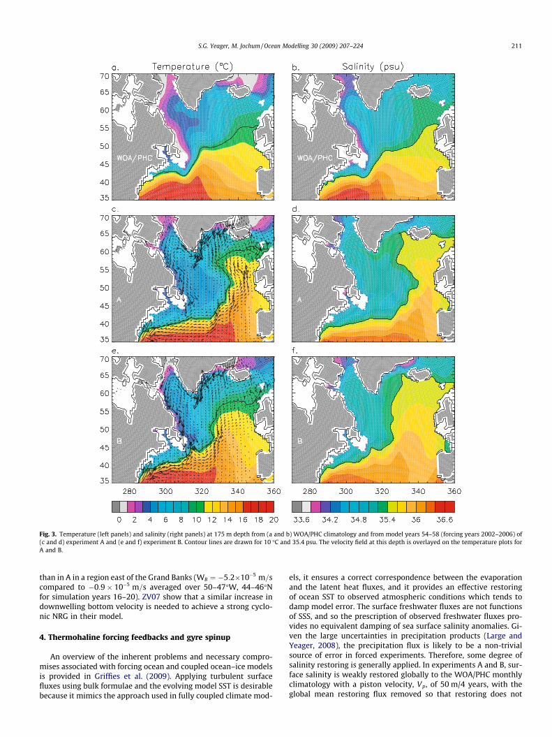
Fig. 3. Temperature (left panels) and salinity (right panels) at 175 m depth from (a and b) WOA/PHC climatology and from model years 54–58 (forcing years 2002–2006) of(c and d) experiment A and (e and f) experiment B. Contour lines are drawn for 10 �C and 35.4 psu. The velocity field at this depth is overlayed on the temperature plots forA and B.


than in A in a region east of the Grand Banks (WB ¼ �5:2�10�5 m=scompared to �0:9� 10�5 m=s averaged over 50–47�W, 44–46�Nfor simulation years 16–20). ZV07 show that a similar increase indownwelling bottom velocity is needed to achieve a strong cyclo-nic NRG in their model.

4. Thermohaline forcing feedbacks and gyre spinup

An overview of the inherent problems and necessary compro-mises associated with forcing ocean and coupled ocean–ice modelsis provided in Griffies et al. (2009). Applying turbulent surfacefluxes using bulk formulae and the evolving model SST is desirablebecause it mimics the approach used in fully coupled climate mod-

els, it ensures a correct correspondence between the evaporationand the latent heat fluxes, and it provides an effective restoringof ocean SST to observed atmospheric conditions which tends todamp model error. The surface freshwater fluxes are not functionsof SSS, and so the prescription of observed freshwater fluxes pro-vides no equivalent damping of sea surface salinity anomalies. Gi-ven the large uncertainties in precipitation products (Large andYeager, 2008), the precipitation flux is likely to be a non-trivialsource of error in forced experiments. Therefore, some degree ofsalinity restoring is generally applied. In experiments A and B, sur-face salinity is weakly restored globally to the WOA/PHC monthlyclimatology with a piston velocity, Vp, of 50 m/4 years, with theglobal mean restoring flux removed so that restoring does not

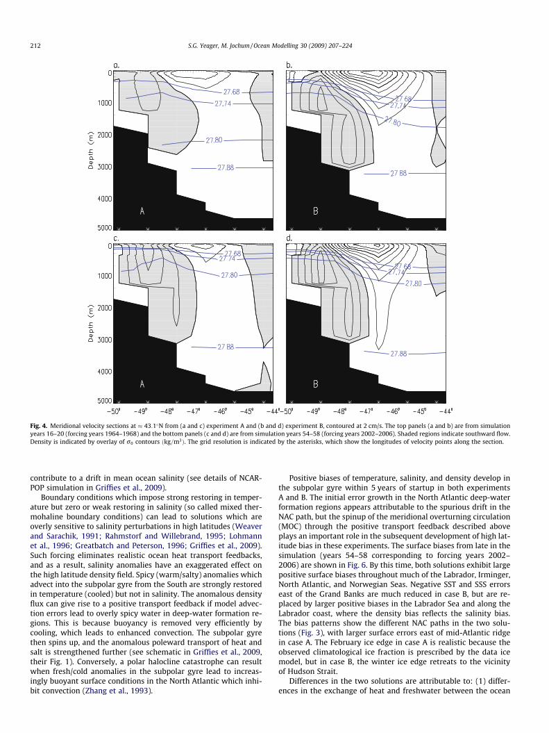
Fig. 4. Meridional velocity sections at � 43:1�N from (a and c) experiment A and (b and d) experiment B, contoured at 2 cm/s. The top panels (a and b) are from simulationyears 16–20 (forcing years 1964–1968) and the bottom panels (c and d) are from simulation years 54–58 (forcing years 2002–2006). Shaded regions indicate southward flow.Density is indicated by overlay of r0 contours ðkg=m3Þ. The grid resolution is indicated by the asterisks, which show the longitudes of velocity points along the section.


contribute to a drift in mean ocean salinity (see details of NCAR-POP simulation in Griffies et al., 2009).

Boundary conditions which impose strong restoring in temper-ature but zero or weak restoring in salinity (so called mixed ther-mohaline boundary conditions) can lead to solutions which areoverly sensitive to salinity perturbations in high latitudes (Weaverand Sarachik, 1991; Rahmstorf and Willebrand, 1995; Lohmannet al., 1996; Greatbatch and Peterson, 1996; Griffies et al., 2009).Such forcing eliminates realistic ocean heat transport feedbacks,and as a result, salinity anomalies have an exaggerated effect onthe high latitude density field. Spicy (warm/salty) anomalies whichadvect into the subpolar gyre from the South are strongly restoredin temperature (cooled) but not in salinity. The anomalous densityflux can give rise to a positive transport feedback if model advec-tion errors lead to overly spicy water in deep-water formation re-gions. This is because buoyancy is removed very efficiently bycooling, which leads to enhanced convection. The subpolar gyrethen spins up, and the anomalous poleward transport of heat andsalt is strengthened further (see schematic in Griffies et al., 2009,their Fig. 1). Conversely, a polar halocline catastrophe can resultwhen fresh/cold anomalies in the subpolar gyre lead to increas-ingly buoyant surface conditions in the North Atlantic which inhi-bit convection (Zhang et al., 1993).

Positive biases of temperature, salinity, and density develop inthe subpolar gyre within 5 years of startup in both experimentsA and B. The initial error growth in the North Atlantic deep-waterformation regions appears attributable to the spurious drift in theNAC path, but the spinup of the meridional overturning circulation(MOC) through the positive transport feedback described aboveplays an important role in the subsequent development of high lat-itude bias in these experiments. The surface biases from late in thesimulation (years 54–58 corresponding to forcing years 2002–2006) are shown in Fig. 6. By this time, both solutions exhibit largepositive surface biases throughout much of the Labrador, Irminger,North Atlantic, and Norwegian Seas. Negative SST and SSS errorseast of the Grand Banks are much reduced in case B, but are re-placed by larger positive biases in the Labrador Sea and along theLabrador coast, where the density bias reflects the salinity bias.The bias patterns show the different NAC paths in the two solu-tions (Fig. 3), with larger surface errors east of mid-Atlantic ridgein case A. The February ice edge in case A is realistic because theobserved climatological ice fraction is prescribed by the data icemodel, but in case B, the winter ice edge retreats to the vicinityof Hudson Strait.

Differences in the two solutions are attributable to: (1) differ-ences in the exchange of heat and freshwater between the ocean

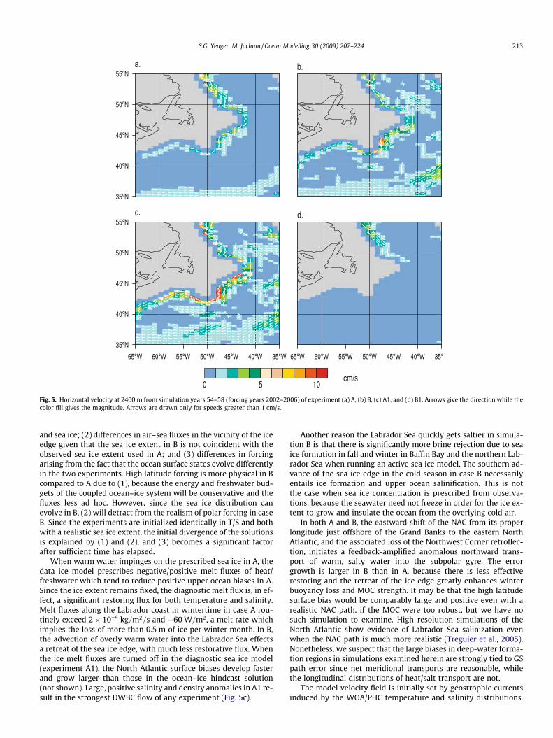
Fig. 5. Horizontal velocity at 2400 m from simulation years 54–58 (forcing years 2002–2006) of experiment (a) A, (b) B, (c) A1, and (d) B1. Arrows give the direction while thecolor fill gives the magnitude. Arrows are drawn only for speeds greater than 1 cm/s.


and sea ice; (2) differences in air–sea fluxes in the vicinity of the iceedge given that the sea ice extent in B is not coincident with theobserved sea ice extent used in A; and (3) differences in forcingarising from the fact that the ocean surface states evolve differentlyin the two experiments. High latitude forcing is more physical in Bcompared to A due to (1), because the energy and freshwater bud-gets of the coupled ocean–ice system will be conservative and thefluxes less ad hoc. However, since the sea ice distribution canevolve in B, (2) will detract from the realism of polar forcing in caseB. Since the experiments are initialized identically in T/S and bothwith a realistic sea ice extent, the initial divergence of the solutionsis explained by (1) and (2), and (3) becomes a significant factorafter sufficient time has elapsed.

When warm water impinges on the prescribed sea ice in A, thedata ice model prescribes negative/positive melt fluxes of heat/freshwater which tend to reduce positive upper ocean biases in A.Since the ice extent remains fixed, the diagnostic melt flux is, in ef-fect, a significant restoring flux for both temperature and salinity.Melt fluxes along the Labrador coast in wintertime in case A rou-tinely exceed 2� 10�4 kg=m2=s and �60 W=m2, a melt rate whichimplies the loss of more than 0.5 m of ice per winter month. In B,the advection of overly warm water into the Labrador Sea effectsa retreat of the sea ice edge, with much less restorative flux. Whenthe ice melt fluxes are turned off in the diagnostic sea ice model(experiment A1), the North Atlantic surface biases develop fasterand grow larger than those in the ocean–ice hindcast solution(not shown). Large, positive salinity and density anomalies in A1 re-sult in the strongest DWBC flow of any experiment (Fig. 5c).

Another reason the Labrador Sea quickly gets saltier in simula-tion B is that there is significantly more brine rejection due to seaice formation in fall and winter in Baffin Bay and the northern Lab-rador Sea when running an active sea ice model. The southern ad-vance of the sea ice edge in the cold season in case B necessarilyentails ice formation and upper ocean salinification. This is notthe case when sea ice concentration is prescribed from observa-tions, because the seawater need not freeze in order for the ice ex-tent to grow and insulate the ocean from the overlying cold air.

In both A and B, the eastward shift of the NAC from its properlongitude just offshore of the Grand Banks to the eastern NorthAtlantic, and the associated loss of the Northwest Corner retroflec-tion, initiates a feedback-amplified anomalous northward trans-port of warm, salty water into the subpolar gyre. The errorgrowth is larger in B than in A, because there is less effectiverestoring and the retreat of the ice edge greatly enhances winterbuoyancy loss and MOC strength. It may be that the high latitudesurface bias would be comparably large and positive even with arealistic NAC path, if the MOC were too robust, but we have nosuch simulation to examine. High resolution simulations of theNorth Atlantic show evidence of Labrador Sea salinization evenwhen the NAC path is much more realistic (Treguier et al., 2005).Nonetheless, we suspect that the large biases in deep-water forma-tion regions in simulations examined herein are strongly tied to GSpath error since net meridional transports are reasonable, whilethe longitudinal distributions of heat/salt transport are not.

The model velocity field is initially set by geostrophic currentsinduced by the WOA/PHC temperature and salinity distributions.

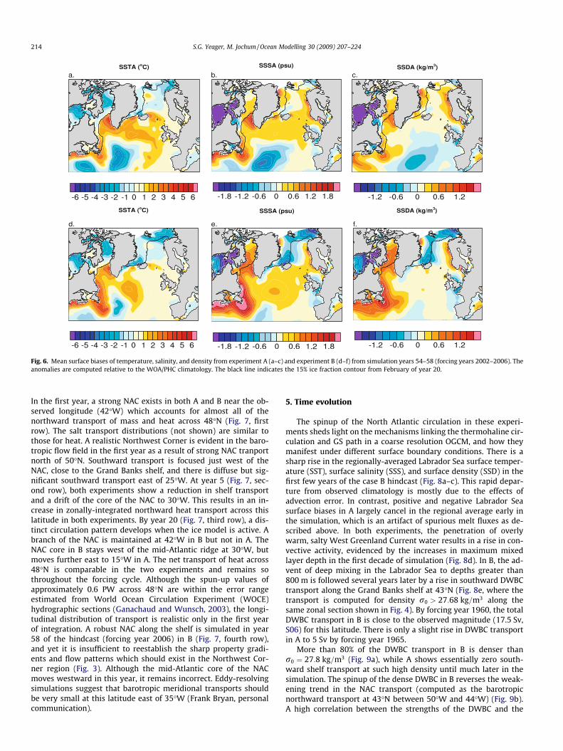
Fig. 6. Mean surface biases of temperature, salinity, and density from experiment A (a–c) and experiment B (d–f) from simulation years 54–58 (forcing years 2002–2006). Theanomalies are computed relative to the WOA/PHC climatology. The black line indicates the 15% ice fraction contour from February of year 20.


In the first year, a strong NAC exists in both A and B near the ob-served longitude (42�W) which accounts for almost all of thenorthward transport of mass and heat across 48�N (Fig. 7, firstrow). The salt transport distributions (not shown) are similar tothose for heat. A realistic Northwest Corner is evident in the baro-tropic flow field in the first year as a result of strong NAC tranportnorth of 50�N. Southward transport is focused just west of theNAC, close to the Grand Banks shelf, and there is diffuse but sig-nificant southward transport east of 25�W. At year 5 (Fig. 7, sec-ond row), both experiments show a reduction in shelf transportand a drift of the core of the NAC to 30�W. This results in an in-crease in zonally-integrated northward heat transport across thislatitude in both experiments. By year 20 (Fig. 7, third row), a dis-tinct circulation pattern develops when the ice model is active. Abranch of the NAC is maintained at 42�W in B but not in A. TheNAC core in B stays west of the mid-Atlantic ridge at 30�W, butmoves further east to 15�W in A. The net transport of heat across48�N is comparable in the two experiments and remains sothroughout the forcing cycle. Although the spun-up values ofapproximately 0.6 PW across 48�N are within the error rangeestimated from World Ocean Circulation Experiment (WOCE)hydrographic sections (Ganachaud and Wunsch, 2003), the longi-tudinal distribution of transport is realistic only in the first yearof integration. A robust NAC along the shelf is simulated in year58 of the hindcast (forcing year 2006) in B (Fig. 7, fourth row),and yet it is insufficient to reestablish the sharp property gradi-ents and flow patterns which should exist in the Northwest Cor-ner region (Fig. 3). Although the mid-Atlantic core of the NACmoves westward in this year, it remains incorrect. Eddy-resolvingsimulations suggest that barotropic meridional transports shouldbe very small at this latitude east of 35�W (Frank Bryan, personalcommunication).

5. Time evolution

The spinup of the North Atlantic circulation in these experi-ments sheds light on the mechanisms linking the thermohaline cir-culation and GS path in a coarse resolution OGCM, and how theymanifest under different surface boundary conditions. There is asharp rise in the regionally-averaged Labrador Sea surface temper-ature (SST), surface salinity (SSS), and surface density (SSD) in thefirst few years of the case B hindcast (Fig. 8a–c). This rapid depar-ture from observed climatology is mostly due to the effects ofadvection error. In contrast, positive and negative Labrador Seasurface biases in A largely cancel in the regional average early inthe simulation, which is an artifact of spurious melt fluxes as de-scribed above. In both experiments, the penetration of overlywarm, salty West Greenland Current water results in a rise in con-vective activity, evidenced by the increases in maximum mixedlayer depth in the first decade of simulation (Fig. 8d). In B, the ad-vent of deep mixing in the Labrador Sea to depths greater than800 m is followed several years later by a rise in southward DWBCtransport along the Grand Banks shelf at 43�N (Fig. 8e, where thetransport is computed for density r0 > 27:68 kg=m3 along thesame zonal section shown in Fig. 4). By forcing year 1960, the totalDWBC transport in B is close to the observed magnitude (17.5 Sv,S06) for this latitude. There is only a slight rise in DWBC transportin A to 5 Sv by forcing year 1965.

More than 80% of the DWBC transport in B is denser thanr0 ¼ 27:8 kg=m3 (Fig. 9a), while A shows essentially zero south-ward shelf transport at such high density until much later in thesimulation. The spinup of the dense DWBC in B reverses the weak-ening trend in the NAC transport (computed as the barotropicnorthward transport at 43�N between 50�W and 44�W) (Fig. 9b).A high correlation between the strengths of the DWBC and the

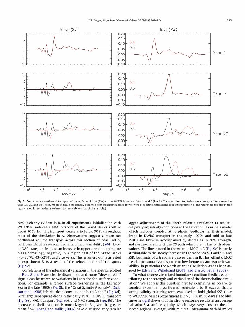
Fig. 7. Annual mean northward transport of mass (Sv) and heat (PW) across 48.3�N from case A (red) and B (black). The rows from top to bottom correspond to simulationyear 1, 5, 20, and 58. The numbers indicate the zonally-summed heat transports across 48�N for the respective simulations. (For interpretation of the references to color in thisfigure legend, the reader is referred to the web version of this article.)


NAC is clearly evident in B. In all experiments, initialization withWOA/PHC induces a NAC offshore of the Grand Banks shelf ofabout 50 Sv, but this transport weakens to below 30 Sv throughoutmost of the simulation in A. Observations suggest a mean netnorthward volume transport across this section of near 140 Sv,with considerable seasonal and interannual variability (S04). Low-er NAC transport leads to an increase in upper ocean temperaturebias (increasingly negative) in a region east of the Grand Banks(45–30�W, 43–52�N), and vice versa. This error growth is arrestedin experiment B as a result of the rejuvenated shelf transports(Fig. 9c).

Correlations of the interannual variations in the metrics plottedin Figs. 8 and 9 are clearly discernible, and some ‘‘downstream”signals can be traced to variations in Labrador Sea surface condi-tions. For example, a forced surface freshening in the LabradorSea in the late 1960s (Fig. 8b, the ‘‘Great Salinity Anomaly”; Dick-son et al., 1988) inhibits deep convection in both A and B (Fig. 8d),with large subsequent drops in the early 1970s in DWBC transport(Fig. 8e), NAC transport (Fig. 9b), and NRG strength (Fig. 9d). Thedecrease in shelf transport is much larger in B, given the greatermean flow. Zhang and Vallis (2006) have discussed very similar

lagged adjustments of the North Atlantic circulation to realisti-cally-varying salinity conditions in the Labrador Sea using a modelwhich includes coupled atmospheric feedbacks. In their model,drops in DWBC transport in the early 1970s and mid to late1980s are likewise accompanied by decreases in NRG strength,and northward shifts of the GS path which are in line with obser-vations. The linear trend in the Atlantic MOC in A (Fig. 9e) is partlyattributable to the steady increase in Labrador Sea SST and SSS andSSD, but hints of a trend are also evident in B. This Atlantic MOCtrend is presumably a response to low frequency atmospheric var-iability, in particular the North Atlantic Oscillation, as has been ar-gued by Eden and Willebrand (2001) and Biastoch et al. (2008).

To what degree are mixed boundary condition feedbacks con-tributing to the strength and variability of the thermohaline circu-lation? We address this question first by examining an ocean–icecoupled experiment configured equivalent to B except that astrong salinity restoring term was used to hold global SSS closeto WOA/PHC values (experiment B1; Vp ¼ 50 m/30 days). The bluecurve in Fig. 8 shows that the strong restoring results in an averageLabrador Sea surface salinity which stays very close to the ob-served regional average, with minimal interannual variability. As

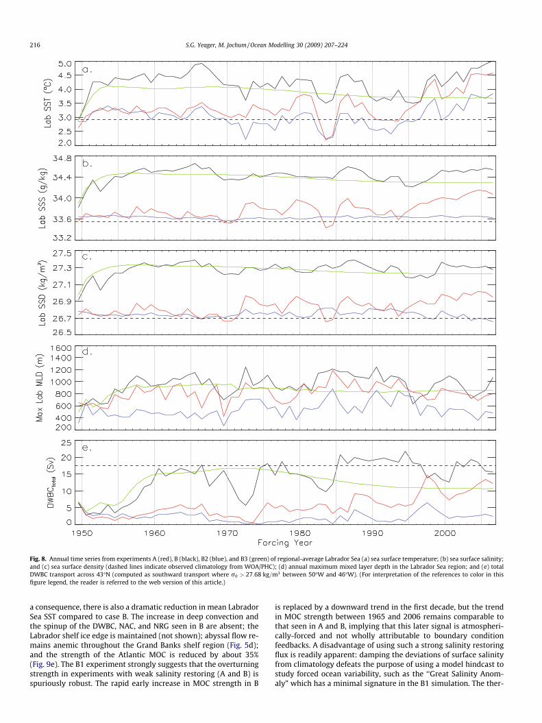
Fig. 8. Annual time series from experiments A (red), B (black), B2 (blue), and B3 (green) of regional-average Labrador Sea (a) sea surface temperature; (b) sea surface salinity;and (c) sea surface density (dashed lines indicate observed climatology from WOA/PHC); (d) annual maximum mixed layer depth in the Labrador Sea region; and (e) totalDWBC transport across 43�N (computed as southward transport where r0 > 27:68 kg=m3 between 50�W and 46�W). (For interpretation of the references to color in thisfigure legend, the reader is referred to the web version of this article.)


a consequence, there is also a dramatic reduction in mean LabradorSea SST compared to case B. The increase in deep convection andthe spinup of the DWBC, NAC, and NRG seen in B are absent; theLabrador shelf ice edge is maintained (not shown); abyssal flow re-mains anemic throughout the Grand Banks shelf region (Fig. 5d);and the strength of the Atlantic MOC is reduced by about 35%(Fig. 9e). The B1 experiment strongly suggests that the overturningstrength in experiments with weak salinity restoring (A and B) isspuriously robust. The rapid early increase in MOC strength in B

is replaced by a downward trend in the first decade, but the trendin MOC strength between 1965 and 2006 remains comparable tothat seen in A and B, implying that this later signal is atmospheri-cally-forced and not wholly attributable to boundary conditionfeedbacks. A disadvantage of using such a strong salinity restoringflux is readily apparent: damping the deviations of surface salinityfrom climatology defeats the purpose of using a model hindcast tostudy forced ocean variability, such as the ‘‘Great Salinity Anom-aly” which has a minimal signature in the B1 simulation. The ther-

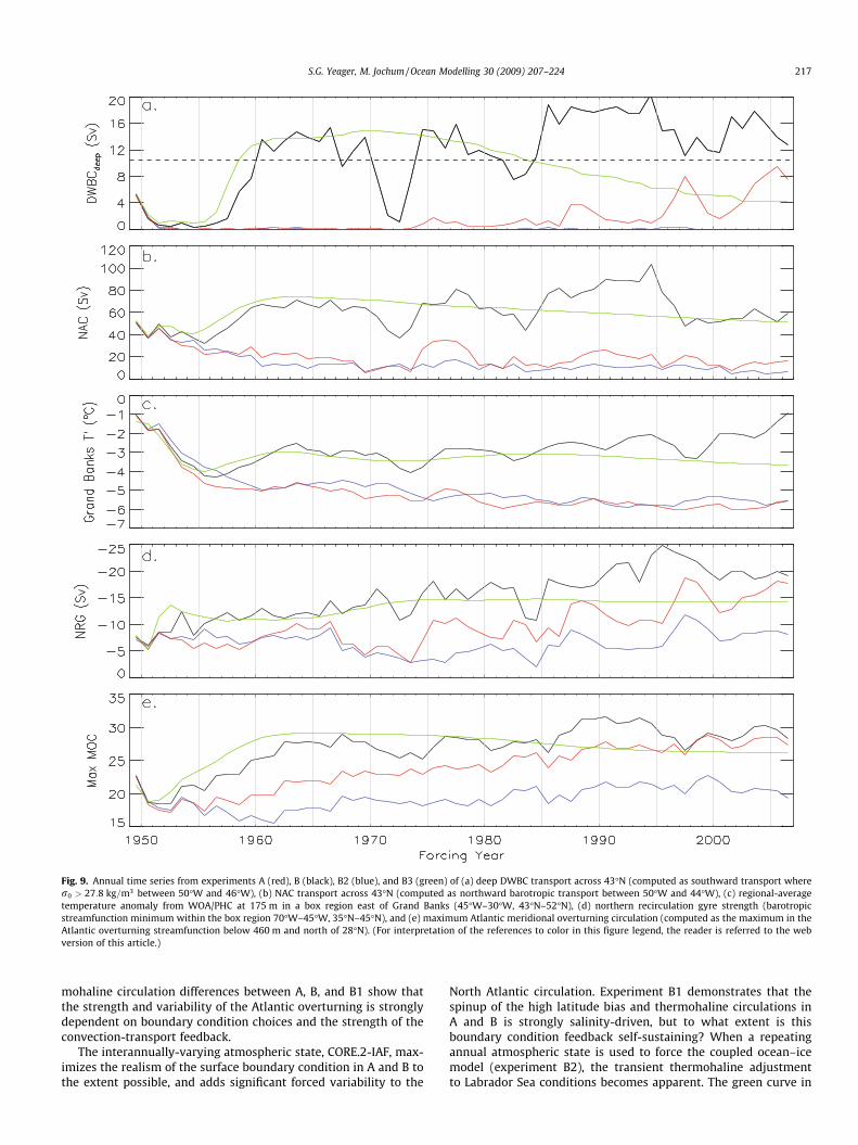
Fig. 9. Annual time series from experiments A (red), B (black), B2 (blue), and B3 (green) of (a) deep DWBC transport across 43�N (computed as southward transport wherer0 > 27:8 kg=m3 between 50�W and 46�W), (b) NAC transport across 43�N (computed as northward barotropic transport between 50�W and 44�W), (c) regional-averagetemperature anomaly from WOA/PHC at 175 m in a box region east of Grand Banks (45�W–30�W, 43�N–52�N), (d) northern recirculation gyre strength (barotropicstreamfunction minimum within the box region 70�W–45�W, 35�N–45�N), and (e) maximum Atlantic meridional overturning circulation (computed as the maximum in theAtlantic overturning streamfunction below 460 m and north of 28�N). (For interpretation of the references to color in this figure legend, the reader is referred to the webversion of this article.)


mohaline circulation differences between A, B, and B1 show thatthe strength and variability of the Atlantic overturning is stronglydependent on boundary condition choices and the strength of theconvection-transport feedback.

The interannually-varying atmospheric state, CORE.2-IAF, max-imizes the realism of the surface boundary condition in A and B tothe extent possible, and adds significant forced variability to the

North Atlantic circulation. Experiment B1 demonstrates that thespinup of the high latitude bias and thermohaline circulations inA and B is strongly salinity-driven, but to what extent is thisboundary condition feedback self-sustaining? When a repeatingannual atmospheric state is used to force the coupled ocean–icemodel (experiment B2), the transient thermohaline adjustmentto Labrador Sea conditions becomes apparent. The green curve in


Fig. 8 shows that the rapid rise in Labrador Sea SSS, SST, and SSDoccurs regardless of the atmospheric boundary conditions whenthe sea ice is prognostic, because inherent ocean model errordrives the initial changes. The spinup of B2 is very comparable toB through simulation year 35, in terms of Labrador Sea surface con-ditions, meridional shelf transports, and gyre strength. After that,the DWBC and MOC in B2 weakens as Labrador Sea surface salinitytrends lower. We conclude that the positive convection feedbackaccounts for most of the variability in the first decades of the Band B2 simulations, but it does not explain the steady increase inDWBC, NRG, and MOC strength seen later in the integration of B(Fig. 9a, d and e). A steady thermohaline circulation is achievedafter roughly 50 years in B2 in which the high latitude salinityand density biases, the DWBC transport, and the gyre strengthare maintained at levels below the early peak.

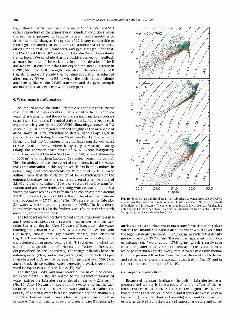
Fig. 10. Temperature-salinity diagram for Labrador Sea water from the WOA/PHCclimatology (top) and from simulation year 50 (historical year 1998) of experimentsA (middle) and B (bottom). The color scheme is as follows (see text for details):entering the Labrador Sea (blue); exiting the Labrador Sea (red); central LabradorSea (green); northern Labrador Sea (black).

6. Water mass transformation

As implied above, the North Atlantic circulation in these coarseresolution OGCM experiments is highly sensitive to Labrador Seawater characteristics and the water mass transformation processesoccurring in this region. The initial state of the Labrador Sea in eachexperiment is given by the WOA/PHC climatology, shown in T-Sspace in Fig. 10. The region is defined roughly as the area west of46�W, north of 50�N, extending to Baffin Island’s Cape Dyer inthe north and excluding Hudson Strait (see Fig. 1). The region isfurther divided into four subregions: entering (along the west coastof Greenland to 65�N, where bathymetry < 3000 m); exiting(along the Labrador coast south of 57�N, where bathymetry< 3000 m); central Labrador Sea (east of 55�W, where bathymetry> 3000 m); and northern Labrador Sea water (remaining points).This climatology reflects the essential characteristics of the watermass transformation in this region which has been examined indetail using float measurements by Palter et al. (2008). Theseauthors show that the distribution of T-S characteristics of theentering boundary current is centered around a temperature of3.8 �C and a salinity value of 34.91. As a result of surface transfor-mation and advective-diffusive mixing with central Labrador Seawater, the water which exits is fresher and cooler, centered around3.4 �C and a salinity value of 34.86. The cluster of exiting water onthe isopycnal r0 ¼ 27:74 kg=m3 (Fig. 10) represents the LabradorSea water which subsequently enters the DWBC. The least denseLabrador Sea water is also the freshest, and is found in the far northand along the Labrador Coast.

The feedback-driven northward heat and salt transport bias in Aand B results in a steady drift in water mass properties in the Lab-rador Sea at all depths. After 50 years of integration, the waterentering the Labrador Sea in case A is almost 2 �C warmer and0.2 saltier, though not significantly denser, than observed(Fig. 10). The exiting water is likewise too warm and salty, and ischaracterized by an unrealistically tight T-S relationship which re-sults from the specification of melt heat and freshwater fluxes un-der prescribed ice (see Appendix A). The change in density betweenentering water (blue) and exiting water (red) is somewhat largerthan observed in A, so that by year 50 (historical year 1998) theanomalously dense exiting water generates a weak deep south-ward transport east of Grand Banks (Fig. 9a).

The stronger DWBC and more realistic NAC in coupled ocean–ice experiments (B, B2) are related to the significant volume ofwater exiting the Labrador Sea at density near r0 ¼ 27:8 kg=m3

(Fig. 10). After 50 years of integration, the water entering the Lab-rador Sea in B is more than 1 �C too warm and 0.2 too saline. Thedensity of entering water is biased positive since the anomalousT and S of the Greenland current is less density-compensating thanin case A. The high density of exiting water in case B is primarily

attributable to a spurious water mass transformation taking placewithin the Labrador Sea. Almost all of the water which advects intothe region at density below r0 ¼ 27:7 kg=m3 advects out at densitygreater than r0 ¼ 27:7 kg=m3. The result is significant productionof Labrador shelf water at r0 ¼ 27:8 kg=m3, which is rarely seenin nature (Palter et al., 2008). The retreat of the Labrador coastice edge contributes to the overly robust water mass transforma-tion in experiment B and explains the prevalence of much denserand saltier water along the Labrador coast (red in Fig. 10) and inthe northern region (black in Fig. 10).

6.1. Surface buoyancy fluxes

Because of transport feedbacks, the drift in Labrador Sea tem-perature and salinity is both a cause of, and an effect of, the re-duced realism of the surface fluxes in this region. Positive SSTbiases in the Labrador Sea in both A and B generate excessive win-ter cooling (primarily latent and sensible) compared to air–sea fluxestimates derived from the observed atmospheric state and corre-


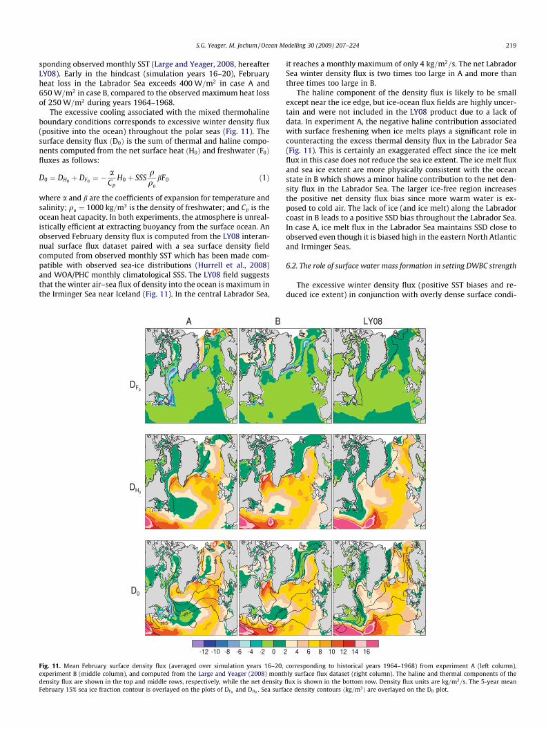
sponding observed monthly SST (Large and Yeager, 2008, hereafterLY08). Early in the hindcast (simulation years 16–20), Februaryheat loss in the Labrador Sea exceeds 400 W=m2 in case A and650 W=m2 in case B, compared to the observed maximum heat lossof 250 W=m2 during years 1964–1968.

The excessive cooling associated with the mixed thermohalineboundary conditions corresponds to excessive winter density flux(positive into the ocean) throughout the polar seas (Fig. 11). Thesurface density flux ðD0Þ is the sum of thermal and haline compo-nents computed from the net surface heat ðH0Þ and freshwater ðF0Þfluxes as follows:

D0 ¼ DH0 þ DF0 ¼ �aCp

H0 þ SSSqqo

bF0 ð1Þ

where a and b are the coefficients of expansion for temperature andsalinity; qo ¼ 1000 kg=m3 is the density of freshwater; and Cp is theocean heat capacity. In both experiments, the atmosphere is unreal-istically efficient at extracting buoyancy from the surface ocean. Anobserved February density flux is computed from the LY08 interan-nual surface flux dataset paired with a sea surface density fieldcomputed from observed monthly SST which has been made com-patible with observed sea-ice distributions (Hurrell et al., 2008)and WOA/PHC monthly climatological SSS. The LY08 field suggeststhat the winter air–sea flux of density into the ocean is maximum inthe Irminger Sea near Iceland (Fig. 11). In the central Labrador Sea,

Fig. 11. Mean February surface density flux (averaged over simulation years 16–20,experiment B (middle column), and computed from the Large and Yeager (2008) montdensity flux are shown in the top and middle rows, respectively, while the net densityFebruary 15% sea ice fraction contour is overlayed on the plots of DF0 and DH0 . Sea surfa

it reaches a monthly maximum of only 4 kg=m2=s. The net LabradorSea winter density flux is two times too large in A and more thanthree times too large in B.

The haline component of the density flux is likely to be smallexcept near the ice edge, but ice-ocean flux fields are highly uncer-tain and were not included in the LY08 product due to a lack ofdata. In experiment A, the negative haline contribution associatedwith surface freshening when ice melts plays a significant role incounteracting the excess thermal density flux in the Labrador Sea(Fig. 11). This is certainly an exaggerated effect since the ice meltflux in this case does not reduce the sea ice extent. The ice melt fluxand sea ice extent are more physically consistent with the oceanstate in B which shows a minor haline contribution to the net den-sity flux in the Labrador Sea. The larger ice-free region increasesthe positive net density flux bias since more warm water is ex-posed to cold air. The lack of ice (and ice melt) along the Labradorcoast in B leads to a positive SSD bias throughout the Labrador Sea.In case A, ice melt flux in the Labrador Sea maintains SSD close toobserved even though it is biased high in the eastern North Atlanticand Irminger Seas.

6.2. The role of surface water mass formation in setting DWBC strength

The excessive winter density flux (positive SST biases and re-duced ice extent) in conjunction with overly dense surface condi-

corresponding to historical years 1964–1968) from experiment A (left column),hly surface flux dataset (right column). The haline and thermal components of theflux is shown in the bottom row. Density flux units are kg=m2=s. The 5-year meance density contours ðkg=m3Þ are overlayed on the D0 plot.


tions (positive SSS biases) leads to overproduction of overly densewater masses in these prescribed atmosphere experiments. Watermass formation driven by air–sea fluxes is determined from thesurface density transformation rate, which is the surface integralof the density influx per unit of density (Speer and Tziperman,1992; Large and Nurser, 2001):

FðqÞ ¼ 1Dq

Zoutcrop

D0dA ð2Þ

The integral is performed over the region bounded by the surfaceoutcrops of q� Dq

2 and qþ Dq2 with Dq ¼ 0:1 kg=m3. The units of

FðqÞ are Sverdrups (Sv). The accumulation of water mass in the den-sity range dq resulting from surface transformation of density isthen given by � @F

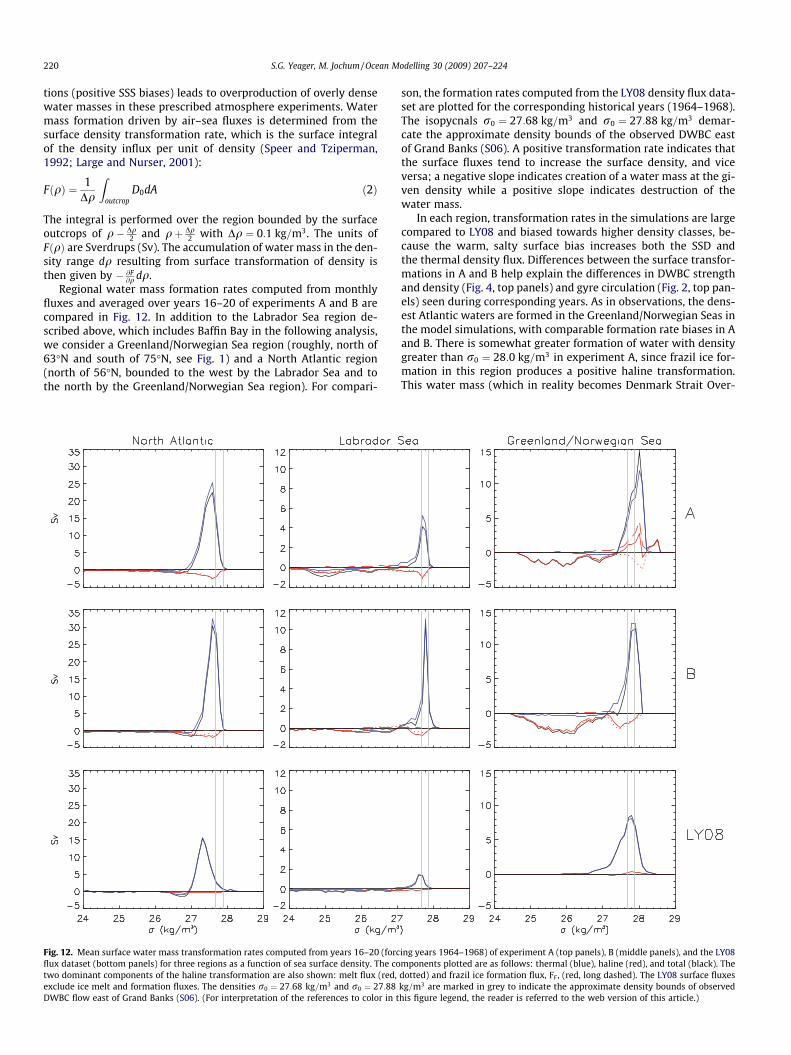
@q dq.Regional water mass formation rates computed from monthly

fluxes and averaged over years 16–20 of experiments A and B arecompared in Fig. 12. In addition to the Labrador Sea region de-scribed above, which includes Baffin Bay in the following analysis,we consider a Greenland/Norwegian Sea region (roughly, north of63�N and south of 75�N, see Fig. 1) and a North Atlantic region(north of 56�N, bounded to the west by the Labrador Sea and tothe north by the Greenland/Norwegian Sea region). For compari-

Fig. 12. Mean surface water mass transformation rates computed from years 16–20 (forcflux dataset (bottom panels) for three regions as a function of sea surface density. The cotwo dominant components of the haline transformation are also shown: melt flux (red,exclude ice melt and formation fluxes. The densities r0 ¼ 27:68 kg=m3 and r0 ¼ 27:88DWBC flow east of Grand Banks (S06). (For interpretation of the references to color in t

son, the formation rates computed from the LY08 density flux data-set are plotted for the corresponding historical years (1964–1968).The isopycnals r0 ¼ 27:68 kg=m3 and r0 ¼ 27:88 kg=m3 demar-cate the approximate density bounds of the observed DWBC eastof Grand Banks (S06). A positive transformation rate indicates thatthe surface fluxes tend to increase the surface density, and viceversa; a negative slope indicates creation of a water mass at the gi-ven density while a positive slope indicates destruction of thewater mass.

In each region, transformation rates in the simulations are largecompared to LY08 and biased towards higher density classes, be-cause the warm, salty surface bias increases both the SSD andthe thermal density flux. Differences between the surface transfor-mations in A and B help explain the differences in DWBC strengthand density (Fig. 4, top panels) and gyre circulation (Fig. 2, top pan-els) seen during corresponding years. As in observations, the dens-est Atlantic waters are formed in the Greenland/Norwegian Seas inthe model simulations, with comparable formation rate biases in Aand B. There is somewhat greater formation of water with densitygreater than r0 ¼ 28:0 kg=m3 in experiment A, since frazil ice for-mation in this region produces a positive haline transformation.This water mass (which in reality becomes Denmark Strait Over-

ing years 1964–1968) of experiment A (top panels), B (middle panels), and the LY08mponents plotted are as follows: thermal (blue), haline (red), and total (black). Thedotted) and frazil ice formation flux, FF , (red, long dashed). The LY08 surface fluxeskg=m3 are marked in grey to indicate the approximate density bounds of observedhis figure legend, the reader is referred to the web version of this article.)


flow Water) may be too dense in the simulations to contribute tothe model DWBC flow east of Grand Banks (Fig. 4). Observations(S06) suggest that there is at least 3.6 Sv of DWBC transport at den-sity greater than r0 ¼ 27:88 kg=m3. This might be better simulatedwith the inclusion of a parameterization for gravity current over-flows, but such a parameterization is lacking in the experimentsexamined here.

Melt fluxes in the Greenland/Norwegian Seas form water in therange from r0 ¼ 25:5 kg=m3 to r0 ¼ 26:0 kg=m3 from denserwater, but this transformation is again comparable in A and Band this density range is too low to contribute to the DWBC. Thepositive thermal density flux biases in the eastern North Atlanticand Irminger Sea region (Fig. 11) are of similar magnitude in bothA and B, and consequently the North Atlantic transformationrates (Fig. 12, left panels) are only slightly different. The largestdifferences in surface water mass transformation rates are in theLabrador Sea (Fig. 12, center panels), where the maximum trans-formation rate is approximately 3 times too large in case A and 7times too large in case B. High thermal density flux over a largearea in B generates a peak transformation rate greater than 10 Svat r0 ¼ 27:8 kg=m3, which accounts for the strong DWBC transportin this density class in the prognostic sea ice experiment (Fig. 4). InA, there is much more negative transformation in the Labrador Sea,corresponding to ice-ocean (melt) flux, which produces lighterwater and maintains a wide spread in the sea surface density. Con-sequently, the production of dense Labrador Sea water via air–seaexchange is confined to a much smaller geographic area in A(Fig. 11), and the peak transformation rate is much lower.

The haline component of the subpolar water mass transforma-tion is much smaller than the thermal component when bulk fluxforcing is used with either diagnostic or prognostic sea ice compo-nent. The negative density flux associated with sea ice melt is thedominant direct effect of the cryosphere on North Atlantic watermass properties. However, the indirect effect of the cryosphereon water mass production, namely the change in the area of directair–sea interaction, is much more significant in the mixed bound-ary condition context, and this effect accounts for the large dis-crepancies in surface transformation (and DWBC transport andGS path) between experiments A and B.

6.3. The effect of salinity restoring boundary conditions

More realistic net transformation rates are seen when strongsalinity restoring is used, as in experiment B1, but only throughof the addition of very large and unphysical haline density fluxes.Since the restoring flux damps the mixed boundary conditiontransport feedback, thereby preserving the Labrador shelf ice edgein the ocean–ice coupled configuration, the thermal transforma-tion rates are much lower in B1 compared to B. They are still highcompared to LY08 since there is still some positive temperaturebias at high latitudes. The salinity restoring flux is large and posi-tive (tending to increase salinity and density) in the Greenland/Norwegian Sea region (not shown), where it counteracts largermelt fluxes in this region associated with increased northward heattransport in the far eastern Atlantic (the transports across 48�N inB1 resemble those from case A). In both the North Atlantic and Lab-rador Sea regions, a negative salinity restoring flux is the dominantterm in the haline transformation, tending to maintain surfacewater of the appropriate climatological density despite advectivesalinity error and excess evaporation. Controlling salinity at theselatitudes thus ensures surface water mass production at the correctdensity and near the correct rate. However, subsurface drift in highlatitude water mass properties associated with circulation errorscontinues even in case B1, such that the Labrador Sea temperatureand salinity distribution bears a strong resemblance to that in Aafter 50 years (Fig. 10).

7. Summary and discussion

With the help of an OGCM, we explore the connection betweenLabrador Sea, DWBC, and the Gulf Stream. Like many authors be-fore, we find that increased buoyancy loss in the Labrador Sea leadsto a strengthening of the DWBC. This then leads to a strongernorthern recirculation gyre, and the subsequent reattachment ofthe Gulf Stream to the Grand Banks. The improved Gulf Streampath significantly reduces negative SST biases in the North Atlantic,which carries with it the hope that future climate simulations canprovide a realistic Jet Stream and north European precipitation.

The ultimate source for the improved Gulf Stream path is thestronger buoyancy loss over the Labrador Sea. Because of themixed boundary conditions, accurate buoyancy loss is strongly tiedto an accurate path of the Gulf Stream and the NAC. Fig. 3 illus-trates that, while case B clearly displays a better NAC position inthe western North Atlantic, in all cases there is an eastward driftof the NAC core which results in spurious northward transport ofwarm and salty Gulf Stream water into the Irminger and LabradorSeas. The ultimate cause for these biases is not known, although itprobably relates to the fact that the mechanism which maintainsthe strong near surface property gradients in the vicinity of theNorthwest Corner is either absent or too weak in these simulations,even when the NAC offshore of Grand Banks is reasonably strong.This clearly warrants further investigation, because the eastwarddrift of northward transports results in the polar seas becomingtoo warm and salty, which is then exacerbated by a strengtheningof the MOC.

If the Labrador Sea sea-ice concentration is restored to the ob-served values (case A), the implied melt water fluxes overcompen-sate for the salty bias, creating too light water and reducingconvection. On the other hand, with a prognostic sea-ice model(case B), the salinity is not artificially changed, but now the warmwater leads to a reduced sea-ice cover and excessive heat loss. Thisleads to an increase in deep ocean convection. These inconsistentresponses are typical for any set of boundary conditions; however,in this particular location it leads to feedbacks which make the sys-tem sensitive to small errors in the salinity field.

In principle, this strong sensitivity could be realistic and oneshould really only be worried about the spurious NAC path in theeast. However, a detailed comparison with observations showsthat the new, much improved dynamics of the western boundarycurrent regime is bought with water mass transformations far be-yond the observed magnitude. Thus, there is a trade-off betweendynamic and thermodynamic fidelity and apparently only onecan be achieved. Strong restoring boundary conditions do not offera satisfactory solution, since there is then neither dynamic northermodynamic fidelity, and although surface biases are reduced,the usefulness of the resulting simulation for studying oceanic var-iability is greatly diminished. In case B, physically consistentocean–ice exchange and a more realistic DWBC/Gulf Stream flowis obtained with excessively large buoyancy losses in the LabradorSea; in case A, spurious air–sea exchange is minimized and the dia-pycnal surface fluxes remain closer to observations, but the surfacetransformation degrades with time and the DWBC is too weak. Thefocus of future research should then be on two topics: Firstly, whatcauses the drift in the NAC path in the central to eastern basin?And secondly, why does it take excessively dense water to createa DWBC of realistic strength?

The first question is closely tied to the surface boundary condi-tions, because the subpolar gyre reaches to the ocean bottom andtherefore is driven by buoyancy forcing and pressure torque asmuch as by the wind (Luyten et al., 1985). Thus, a slight bias inthe NAC path may be amplified by the interaction with the bottomtopography and mismatched boundary conditions. Semi-prognos-


tic methods which nudge the pressure field towards climatology inthe Northwest Corner region lead to better NAC simulation in thisclass of model (Greatbatch et al., 2004; Weese and Bryan, 2006),suggesting that a better understanding of the mechanisms whichsustain the pressure gradient would help direct the effort to simu-late it correctly. We postulate that deficient initial conditions mayalso play a role in NAC detachment: since the ocean is initializedfrom rest, a geostrophic NAC is generated from the start, but theDWBC starts out very weak and quickly diminishes (Figs. 8 and9), until a decade of simulation has elapsed in B. Given the dearthof deep velocity observations and the biases inherent in any coarseresolution OGCM velocity field, it is unclear how one could pre-scribe an adequate initial velocity field which might prevent theNAC drift in the first place.

The second question, or the question ‘‘what determines DWBCstrength and position?”, is amply discussed in the literature. Apartfrom Labrador Sea buoyancy fluxes, it depends on abyssal upwell-ing (Stommel and Arons, 1960), strength of Arctic overflows (War-ren, 1981), vertical eddy fluxes (Bryan et al., 2007), and shape ofthe bottom topography (ZV07). However, all of these are highlyresolution dependent and not easily changed in a global OGCM.Increasing the abyssal upwelling and subsequent strengtheningof the DWBC can be achieved by increased diapycnal diffusivity(Jochum, 2008), but its value is strongly constrained by globalconsiderations (Menemenlis et al., 2005). The weakness of themodeled DWBC is probably partly related to insufficiently repre-sented Arctic overflows, but the densest DWBC flow accounts fora relatively small fraction of the total (S06). Preliminary experi-ments with an overflow parameterization included in the most re-cent CCSM ocean model do not show significant enhancement ofDWBC flow to the east and south of the Grand Banks (GokhanDanabasoglu, personal communication). Vertical eddy fluxes asparameterized by Gent and McWilliams (1990) promise some con-trol, but in practice the need to find a parameterization that pro-vides a reasonable ACC transport puts a strong constraint on itsstructure (Eden et al., 2009). Thus, the present study, like many be-fore it, suggests that while it is possible in principle to find physi-cally-based controls for the OGCM representation of Gulf Streamand DWBC, in practice so many different sub-gridscale processeswould have to be parameterized and tuned properly for the NorthAtlantic that the global fidelity of any OGCM is likely to suffer.

Finding a means to control DWBC strength is hindered by thefact that OGCMs with or without sea ice models suffer from themismatch between observed atmospheric forcing and the modeledGulf Stream position. Atmospheric models from coupled GCMs onthe other hand, do not typically have the required resolution tocreate the strong storms with their large buoyancy loss whichwould seem to be necessary for realistic Labrador Sea water pro-duction. Thus, while the present study offers a glimmer of hopethat the Gulf Stream path can be improved upon in climate models,it may well be that we will only be able to choose the nature of ourbiases. For example, for a climate study with less than 100 yearduration, choosing the DWBC density biases over the Gulf Streamseparation biases is an attractive choice because it will improvesurface climate over the North Atlantic. For longer studies, how-ever, it can be anticipated that the DWBC biases affect the densitystructure of the world ocean, and one will want to chose accurateNADW density over good Gulf Stream separation.

In this study, we demonstrate a link between Labrador Sea deepconvection and Gulf Stream path in the non-eddy resolving oceanmodel component of the CCSM. As in the previous work of Zhangand Vallis (2006, 2007), we find that a strong, dense, downslopeDWBC couples the thermohaline circulation to the gyre circulationin the North Atlantic via vortex stretching in the Grand Banks shelfregion. The simulated DWBC is highly sensitive to high latitudesurface boundary conditions, and in particular to salinity condi-

tions in the Labrador Sea, and is generally anemic unless tempera-ture and salinity in the subpolar gyre deviate significantly fromobserved values. The magnitude of high latitude temperature andsalinity biases in the North Atlantic, and consequently the strengthof the DWBC and the NAC path, is shown to be strongly dependenton the choice of sea ice and salinity restoring boundary conditions.The primary conclusions of this study are as follows:

� High surface production of dense water in the Labrador Seaimproves the North Atlantic circulation by generating a stronger,more realistic DWBC on the Grand Banks shelf which maintainsa reasonable offshore NAC. As a result, general improvementsare seen in the barotropic streamfunction and upper ocean tem-perature and salinity.

� Feedbacks associated with mixed surface boundary conditionsresult in unrealistically strong surface production of the densestNorth Atlantic water masses in CCSM 3.5 configurations of the 1�POP ocean model driven by a prescribed atmosphere. The feed-backs linking thermohaline forcing and gyre circulation arestrengthened when a prognostic sea ice model is used, particu-larly when historical forcing is applied, and weakened whenstrong salinity restoring is used.

� There is a strong convolution of model error with diapycnal sur-face flux error in the North Atlantic which implies a low fidelityof hindcast thermohaline circulation variations in the Atlanticbasin.

Acknowledgments

Helpful feedback from Peter Gent and two anonymous review-ers is gratefully acknowledged. We also thank Bill Large for theencouragement to pursue this research. This work was supportedby the National Science Foundation through its sponsorship ofthe National Center for Atmospheric Research.

Appendix A. Data sea ice model

In the data ice model used for ocean only experiments, daily ob-served sea ice fraction obtained from the Special Sensor Micro-wave/Imager (SSM/I) (Comiso, 1999) defines fSSMI at each modelgrid point. This areal coverage represents the only historicalboundary condition in regions of sea ice, since under ice fluxesassociated with sea ice melt (M), frazil ice formation (F), basal iceformation (B), and penetrating solar radiation (PS) are neither wellconstrained by observations nor amenable to specification throughbulk formulae. Therefore, a crude heat budget is used to derivethese fluxes in ocean only experiments. Following Large and Yea-ger (2004), the components of heat and freshwater exchange be-tween the ice and ocean are:

Qio ¼Q M þ QF þ QB þ QPS ð3ÞFio ¼FM þ FF þ FB ð4Þ

When temperatures fall below freezing in the uppermost layerof the ocean model, temperature and salinity are adjusted by frazilice formation fluxes which return the temperature to freezingwithin a timestep Dt, with an associated negative freshwater fluxrepresenting brine rejection:

QF ¼qoCpðhf � h1ÞD1zDt�1 ð5ÞFF ¼� QFK

�1f ð6Þ

In the above, qo ¼ 1026 kg=m3 is the density of sea water,Cp ¼ 3996 J kg�1 K�1 is the heat capacity of sea water, hf ¼ �1:8 �Cis the freezing point of sea water, h1 is the temperature of the first


model layer, D1z ¼ 10 m is the thickness of the first model layer,and Kf ¼ 333;700 J kg�1 is the latent heat of fusion. If the frazilice forms where observed fSSMI ¼ 0, the frozen water content is accu-mulated locally and a fractional ice coverage is prescribed accordingto

W ¼ �FFDt ð7Þffrazil ¼ minð1:0;W=WmaxÞ ð8Þ

where Wmax ð¼ 1000 kg=m2Þ is the water content threshold corre-sponding to complete grid cell coverage assuming an ice thicknessof 1 meter. The air–sea fluxes of heat and freshwater derived frombulk formulae are applied only where ð1� ficeÞ is non-zero, where

fice ¼ fSSMI þ ffrazil ð9Þ

Momentum fluxes pass from air to sea regardless of ice coverage.Whenever QF > 0, frazil ice is formed in the model and melt

fluxes are set to zero ðQ M ¼ FM ¼ 0Þ. When QF < 0, the frazil iceformation terms are replaced by non-zero melt fluxes as long assurface ice exists ðfice > 0Þ. The amount of ice available for meltingis considered infinite when fSSMI > 0, but is limited by W whenfSSMI ¼ 0. The negative heat and positive freshwater melt fluxesare thus

Q M ¼ maxðQ F ;Q minÞ; fSSMI > 0 ð10ÞQ M ¼ maxðQ F ;Q min;�WKf Dt�1Þ; fSSMI ¼ 0 ð11ÞFM ¼ �QMK�1

f ð12Þ

In the above, Qmin specifies a maximum melt rate generally set to�300 W=m2. If melt occurs where fSSMI ¼ 0, the accumulated frazilice content ðWÞ is reduced by FMDt. If frazil ice formation occurswhere fSSMI > 0, any accumulated frazil ice is eliminated ðW ¼ 0Þ.

In the implementation of the data ice model used herein, thepenetrating shortwave, QPS, and basal ice formation, QB, heat fluxesare set to zero, and the freshwater flux associated with basal iceformation, FB, is prescribed from a monthly climatology obtainedfrom a coarse resolution coupled ocean–ice simulation (Danabaso-glu, 2004). This method was simple and deemed preferable toneglecting the basal terms altogether, but alternative treatmentscould be advocated given the large inherent uncertainties in spec-ifying under-ice boundary conditions for uncoupled ocean models.

References

Biastoch, A., Boning, C., Getzlaff, J., Molines, J-M., Madec, G., 2008. Causes ofinterannual-decadal variability in the meridional overturning circulation of themid-latitude North Atlantic Ocean. J. Climate 21, 6599–6615.

Brachet, S., Le Traon, P.Y., Le Provost, C., 2004. Mesoscale variability from a high-resolution model and from altimeter data in the North Atlantic Ocean. J.Geophys. Res. 109. doi:10.1029/2004JC002360.

Bryan, F.O., Hecht, M.W., Smith, R.D., 2007. Resolution convergence and sensitivitystudies with North Atlantic circulation models. Part I: the western boundarycurrent system. Ocean Modell. 16, 141–159.

Comiso, J., 1999. Bootstrap Sea Ice Concentrations for NIMBUS-7 SMMR and DMSPSSM/I. Digital Media, National Snow and Ice Data Center.

Dai, A.G., Hu, A., Meehl, G.A., Washington, W.M., Strand, W.G., 2005. Atlanticthermohaline circulation in a coupled general circulation model: unforcedvariations versus forced changes. J. Climate 18, 2990–3013.

Danabasoglu, G., 2004. A comparison of global ocean general circulation modelsolutions obtained with synchronous and accelerated integration methods.Ocean Modell. 7, 323–341.

Danabasoglu, G., Large, W.G., Tribbia, J.J., Gent, P.R., Briegleb, B.P., 2006. Diurnalcoupling in the Tropical oceans of CCSM3. J. Climate 19, 2347–2365.

Danabasoglu, G., Marshall, J., 2007. Effects of vertical variations of thicknessdiffusivity in an ocean general circulation model. Ocean Modell. 18, 122–141.

Danabasoglu, G., Ferrari, R., McWilliams, J.C., 2008. Sensitivity of an ocean generalcirculation model to a parameterization of near-surface eddy fluxes. J. Climate21, 1192–1208.

Dengg, J., Beckmann, A., Gerdes, R., 1996. The Gulf Stream separation problem. In:Krauss, W. (Ed.), The Warmwatersphere of the North Atlantic Ocean. Gebr.Borntraeger, pp. 253–290.

Dickson, R.R., Meincke, J., Malmberg, S.-A., Lee, A.J., 1988. The great salinity anomalyin the northern North Atlantic 1968–1982. Prog. Oceanogr. 20, 103–151.

Doney, S.C., Yeager, S.G., Danabasoglu, G., Large, W.G., McWilliams, J.C., 2003.Modeling Global Oceanic Inter-annual Variability (1958–1997): SimulationDesign and Model-data Evaluation. Technical Report TN-452+STR, NCAR, pp. 48.

Dukowicz, J.K., Smith, R.D., 1994. Implicit free-surface formulation of the Bryan–Cox–Semtner ocean model. J. Geophys. Res. 99, 7991–8014.

Eden, C., Jochum, M., Danabasoglu, G., 2009. Effects of different closures forthickness diffusivity. Ocean Modell. 26, 47–59.

Eden, C., Willebrand, J., 2001. Mechanism of interannual to decadal variability of theNorth Atlantic circulation. J. Climate 14, 2266–2280.

Ezer, T., Mellor, G.L., 1992. A numerical study of the variability and separation of theGulf Stream, induced by surface atmospheric forcing and lateral boundaryflows. J. Phys. Oceanogr. 22, 660–682.

Ferrari, R., McWilliams, J.C., Canuto, V.M., Dubovikov, M., 2008. Parameterization ofeddy fluxes near oceanic boundaries. J. Climate 21, 2770–2789.

Ganachaud, A., Wunsch, C., 2003. Large-scale ocean heat and freshwater transportsduring the world ocean circulation experiment. J. Climate 16, 696–705.

Gent, P.R., McWilliams, J.C., 1990. Isopycnal mixing in ocean circulation models. J.Phys. Oceanogr. 20, 150–155.

Gerdes, R., Koberle, C., 1995. On the influence of DSOW in a numerical model of theNorth Atlantic General Circulation. J. Phys. Oceanogr. 25, 2624–2642.

Griffies, S.M., Biastoch, A., Boning, C., Bryan, F., Danabasoglu, G., Chassignet, E.P.,England, M.H., Gerdes, R., Haak, H., Hallberg, R.W., Hazeleger, W., Jungclaus, J.,Large, W.G., Madec, G., Pirani, A., Samuels, B.L., Scheinert, M., Gupta, A.S.,Severijns, C.A., Simmons, H.L., Treguier, A.M., Winton, M., Yeager, S.G., Yin, J.,2009. Coordinated ocean–ice reference experiments (COREs). Ocean Modell. 26,1–46.

Greatbatch, R.J., Peterson, K.A., 1996. Interdecadal variability and oceanicthermohaline adjustment. J. Geophys. Res. 101, 20467–20482.

Greatbatch, R.J., Sheng, J., Eden, C., Tang, L., Zhai, X., Zhao, J., 2004. The semi-prognostic method. Cont. Shelf Res. 24, 2149–2165.

Hogg, N.G., Pickart, R.S., Hendry, R.M., Smethie Jr., W.M., 1986. The northernrecirculation gyre of the Gulf Stream. Deep-Sea Res. 33, 1139–1165.

Holland, M.M., Bitz, C.M., Hunke, E.C., Lipscomb, W.H., Schramm, J.L., 2006.Influence of the sea ice thickness distribution on polar climate in CCSM3. J.Climate 19, 2398–2414.

Huffman, G., Adler, R., Arkin, P., Chang, A., Ferraro, R., Gruber, R., Janowiak, J.,McNab, A., Rudolf, B., Schneider, U., 1997. The global precipitation climatologyproject (GPCP) combined precipitation data set. Bull. Am. Meteor. Soc. 78, 5–20.

Hurlburt, H.E., Hogan, P.J., 2000. Impact of 1/8� to 1/64� on Gulf Stream model-datacomparisons in basin-scale subtropical Atlantic Ocean models. Dyn. Atmos.Oceans 32, 283–330.

Hurrell, J., Hack, J., Shea, D., Caron, J., Rosinski, J., 2008. A new sea surfacetemperature and sea ice boundary data set for the Community AtmosphereModel. J. Climate 19, 5145–5153.

Jayne, S.R., 2009. The impact of abyssal mixing parameterizations in an oceangeneral circulation model. J. Phys. Oceanogr. 39, 1756–1775.

Jochum, M., Danabasoglu, G., Holland, M., Kwon, Y.-O., Large, W.G., 2008. Oceanviscosity and climate. J. Geophys. Res. 113. doi:10.1029/2007JC004515.

Jochum, M., 2008. The impact of latitudinal variations in vertical diffusivity onclimate simulations. J. Geophys. Res. 114. doi:10.1029/2008JC005030.

Joyce, T.M., Deser, C., Spall, M.A., 2000. The relation between decadal variability ofsubtropical mode water and North Atlantic oscillation. J. Climate 13, 2550–2569.

Kalnay, E., Kanamitsu, M., Kistler, R., Collins, W., Deaven, D., Gandin, L., Iredell, M.,Saha, S., White, G., Woollen, J., Zhu, Y., Chelliah, M., Ebisuzaki, W., Higgins, W.,Janowiak, J., Mo, K., Ropelewski, C., Leetma, A., Reynolds, R., Jenne, R., 1996. TheNCEP/NCAR 40-year reanalysis project. Bull. Am. Meteor. Soc. 77, 437–471.

Large, W.G., Danabasoglu, G., Doney, S.C., McWilliams, J.C., 1997. Sensitivity tosurface forcing and boundary layer mixing in a global ocean model: annual-mean climatology. J. Phys. Oceanogr. 27, 2418–2447.

Large, W.G., Danabasoglu, G., McWilliams, J.C., Gent, P., Bryan, F.O., 2001. Equatorialcirculation of a global ocean climate model with anisotropic horizontalviscosity. J. Phys. Oceanogr. 31, 518–536.

Large, W.G., Nurser, G., 2001. Ocean Surface Water Mass Transformation. OceanCirculation and Climate. Academic Press. pp. 317–336 (Chapter 5.1).

Large, W.G., Yeager, S.G., 2004. Diurnal to Decadal Global Forcing for Ocean and Sea-ice Models: The Data Sets and Flux Climatologies. Technical Report TN-460+STR. NCAR, pp. 105.

Large, W.G., Danabasoglu, G., 2006. Attribution and impacts of upper-ocean biasesin CCSM3. J. Climate 19, 2325–2346.

Large, W.G., Yeager, S.G., 2008. The global climatology of an interannually varyingair–sea flux dataset. Clim. Dyn. doi:10.1007/s00382-008-0441-3.

Levitus, S., Boyer, T., Conkright, M., Johnson, D., O’Brien, T., Antonov, J., Stephens, C.,Gelfeld, R., 1998. Introduction, vol. 1. World Ocean Database 1998, NOAA AtlasNESDIS 18, pp. 346.

Lohmann, G., Gerdes, R., Chen, D., 1996. Sensitivity of the thermohaline circulationin coupled oceanic GCM – atmospheric EBM experiments. Clim. Dyn. 12, 403–416.

Luyten, J., Stommel, H., Wunsch, C., 1985. A diagnostic study of the northernAtlantic subpolar gyre. J. Phys. Oceanogr. 15, 1344–1348.

Menemenlis, D., Fukumori, I., Lee, T., 2005. Using Green’s functions to calibrate anocean general circulation model. Mon. Wea. Rev. 133, 1224–1240.

Oschlies, A., 2002. Improved representation of upper-ocean dynamics and mixed-layer depths in a model of the North Atlantic on switching from eddy-permitting to eddy resolving grid resolution. J. Phys. Oceanogr. 32, 2277–2298.

http://dx.doi.org/10.1029/2004JC002360

http://dx.doi.org/10.1029/2007JC004515

http://dx.doi.org/10.1029/2008JC005030

http://dx.doi.org/10.1007/s00382-008-0441-3


Palter, J.B., Lozier, M.S., Lavender, K.L., 2008. How does Labrador Sea water enter thedeep western boundary current? J. Phys. Oceanogr. 38, 968–983.

Rahmstorf, S., Willebrand, J., 1995. The role of temperature feedback in stabilizingthe thermohaline circulation. J. Phys. Oceanogr. 25, 787–805.

Rossby, T., 1996. The North Atlantic Current and surrounding waters: at thecrossroads. Rev. Geophys. 34, 463–481.

Schmitz, W.J., McCartney, M.S., 1993. On the North Atlantic Circulation. Rev.Geophys. 31, 29–49.

Schott, F.A., Zantopp, R., Stramma, L., Dengler, M., Fischer, J., Wibaux, M., 2004.Circulation and deep-water export at the western exit of the subpolar NorthAtlantic. J. Phys. Oceanogr. 34, 817–843.

Schott, F.A., Fischer, J., Dengler, M., Zantopp, R., 2006. Variability of the deepwestern boundary current east of the Grand Banks. Geophys. Res. Lett. 33.doi:10.1029/2006GL026563.

Smith, R.D., Dukowicz, J.K., Malone, R.C., 1992. Parallel ocean general circulationmodeling. Physica D 60, 38–61.

Smith, R.D., Maltrud, M.E., Bryan, F.O., Hecht, M.W., 2000. Numerical simulation ofthe North Atlantic Ocean at 1/10�. J. Phys. Oceanogr. 30, 1532–1561.

Spall, M.A., 1996. Dynamics of the Gulf Stream/deep western boundary currentcrossover. Part I: entrainment and recirculation. J. Phys. Oceanogr. 26, 2152–2168.

Speer, K., Tziperman, E., 1992. Rates of water mass formation in the North AtlanticOcean. J. Phys. Oceanogr. 22, 93–104.

Steele, M., Morley, R., Ermold, W., 2001. PHC: a global ocean hydrography with ahigh-quality Arctic Ocean. J. Climate 14, 2079–2087.

Stommel, H., Arons, A.B., 1960. On the abyssal circulation of the world ocean. I.Stationary planetary flow patterns on a sphere. Deep-Sea Res. 6, 140–154.

Tansley, C.E., Marshall, D.P., 2000. On the influence of bottom topography and thedeep western boundary current on Gulf Stream separation. J. Mar. Res. 58, 297–325.

Thompson, J.D., Schmitz, W.J., 1989. A limited area model of the Gulf Stream:design, initial experiments and model data intercomparison. J. Phys. Oceanogr.19, 791–814.

Treguier, A.M., Theetten, S., Chassignet, E.P., Penduff, T., Smith, R., Talley, L.,Beismann, J.O., Boning, C., 2005. The North Atlantic subpolar gyre in four high-resolution models. J. Phys. Oceanogr. 35, 757–774.

Warren, B.A., 1981. Deep Circulation of the World Ocean. Evolution in PhysicalOceanography. MIT Press. pp. 6–41.

Weaver, A.J., Sarachik, E.S., 1991. Evidence for decadal variability in an oceancirculation model: an advective mechanism. Atmos. Ocean 29, 197–231.

Weese, S.R., Bryan, F.O., 2006. Climate impacts of systematic errors in thesimulation of the path of the North Atlantic Current. Geophys. Res. Lett. 33.doi:10.1029/2006GL027669.

Xie, P., Arkin, P.A., 1996. Analyses of global monthly precipitation using gaugeobservations, satellite estimates, and numerical model predictions. J. Climate 9,840–858.

Zhang, S., Greatbatch, R.J., Lin, C.A., 1993. A reexamination of the polar haloclinecatastrophe and its implications for couple ocean–atmosphere modeling. J.Phys. Oceanogr. 23, 287–299.

Zhang, Y., Rossow, W., Lacis, A., Oinas, V., Mishchenko, M., 2004. Calculation ofradiative flux profiles from the surface to top-of-atmosphere based on ISCCPand other global data sets: refinements of the radiative transfer model andinput data. J. Geophys. Res. 109. doi:10.1029/2003JD004457.

Zhang, R., Vallis, G.K., 2006. Impact of great salinity anomalies on the low-frequencyvariability of the North Atlantic Current. J. Climate 19, 470–482.

Zhang, R., Vallis, G.K., 2007. The role of bottom vortex stretching on the path of theNorth Atlantic western boundary current and on the northern recirculationgyre. J. Phys. Oceanogr. 37, 2053–2080.

http://dx.doi.org/10.1029/2006GL026563

http://dx.doi.org/10.1029/2006GL027669

http://dx.doi.org/10.1029/2003JD004457

Documents

The connection between Labrador Sea buoyancy loss, deep