IZA DP No. 1162

The Connexion between Old and NewApproaches to Financial Satisfaction

Bernard M. S. van Praag

DI

SC

US

SI

ON

PA

PE

R S

ER

IE

S

Forschungsinstitutzur Zukunft der ArbeitInstitute for the Studyof Labor

May 2004

The Connexion between Old and New Approaches to Financial Satisfaction

Bernard M. S. van Praag University of Amsterdam, Tinbergen Institute

and IZA Bonn

Discussion Paper No. 1162 May 2004

(revised: August 2006)

IZA

P.O. Box 7240 53072 Bonn

Germany

Phone: +49-228-3894-0 Fax: +49-228-3894-180

Email: iza@iza.org

Any opinions expressed here are those of the author(s) and not those of the institute. Research disseminated by IZA may include views on policy, but the institute itself takes no institutional policy positions. The Institute for the Study of Labor (IZA) in Bonn is a local and virtual international research center and a place of communication between science, politics and business. IZA is an independent nonprofit company supported by Deutsche Post World Net. The center is associated with the University of Bonn and offers a stimulating research environment through its research networks, research support, and visitors and doctoral programs. IZA engages in (i) original and internationally competitive research in all fields of labor economics, (ii) development of policy concepts, and (iii) dissemination of research results and concepts to the interested public. IZA Discussion Papers often represent preliminary work and are circulated to encourage discussion. Citation of such a paper should account for its provisional character. A revised version may be available on the IZA website (www.iza.org) or directly from the author.

IZA Discussion Paper No. 1162 May 2004 (revised: August 2006)

ABSTRACT

The Connexion between Old and New Approaches to Financial Satisfaction∗

In this paper we compare the new satisfaction evaluation approach, developed in the nineties by Oswald, Clark, Blanchflower and others with the older income evaluation (IEQ) approach, developed by Van Praag and Kapteyn in the seventies of the previous century. We find that both approaches yield strikingly similar results with respect to financial satisfaction. The IEQ- approach yields additional insights, but it is not well applicable to other life domains than finance. It is argued that the usual Probit specification implies a specific cardinalization and, consequently, is less ordinal than usually thought. It is shown that the Probit-approach may be replaced by three other equivalent specifications that have some computational and intuitive advantages. JEL Classification: C24, C25, D31, H31, I31, I39 Keywords: financial satisfaction, income evaluation, Probit-models, cardinal utility Bernard M.S. van Praag Faculty of Economics and Econometrics University of Amsterdam Roetersstraat 11 1018 WB Amsterdam The Netherlands Email: B.M.S.vanPraag@uva.nl

∗ This paper is partly based on Chapter 2 of Happiness Quantified: A Satisfaction Calculus Approach (2004) by B.M.S. Van Praag and A. Ferrer-i-Carbonell.

3

THE CONNEXION BETWEEN OLD AND NEW APPROACHES TO FINANCIAL SATISFACTION

by

Bernard M.S.van Praag*

1. Introduction

The subject 'happiness' of this timely book is one of the most pressing ones for the

behavioural sciences in general and for economics in particular. As I am an economist

by upbringing, I will restrict myself mostly to the economic viewpoint, although it is

clearly unavoidable that there will be points of tangency with the other behavioural

sciences, especially with psychology.

Economists agree on the fact that individuals strife for the greatest happiness. Let us

assume two situations x1 and x2 and let us assume that the two situations generate

happiness values W1 and W2 , where W2 > W1 , then the individual will choose x2 , if

that situation is in his choice set. It follows that the function W(x) describes a very

basic aspect of human behaviour. Choice between scarce things is the core subject of

economics.

It is therefore normal that economists developed this choice model, where human

choice behaviour is described as maximizing a function W on a relevant choice set.

One of the first economists who proposed it was Edgeworth in his book Mathematical

Psychics (1881). He thought of W as a cardinal concept. If W(x1)=1 and W(x2)=2, then

the individual derives twice as much utility1 (or happiness) from x2 as from x1.

Pareto(1904) was the first to raise doubts about the practical possibility to observe and

estimate the function W. Moreover, he showed that in the case of static consumer

behaviour we do not need to know the function itself but only its contour lines, the so

– called indifference curves, which are described by the equations:

* The author is university professor at the University of Amsterdam. This paper is partly based on Chapter 2 of Happiness Quantified : A Satisfaction Calculus Approach (2004) by B.M.S. Van Praag and A. Ferrer-i-Carbonell.

4

( )W x C= (1)

where C stands for a constant. The same net of indifference curves is described by

( ( )) ( )W x Cϕ ϕ= (2)

where ϕ (.) stands for an arbitrary monotonously increasing function.

The net of indifference curves defines an equivalence class of functions ( ( ))W xϕ ,

that have the same contour lines.

In the meantime there arose a growing aversion among economists towards

'psychologizing'. The term 'happiness' was abandoned for 'ophelimity ' and later on for

'well –being ', 'welfare ' or for the still less emotionally loaded term 'utility' or

'satisfaction'.

The practical difficulty to estimate the function W was annoying for economists and

it led to the gradual coming –up of the axiom that utility was immeasurable. Notice

that an axiom is not proven but proposed and accepted. The high priest of this dogma

was Lionel Robbins (1932) and it was supported by Hicks (1939), Samuelson (1947)

and Houthakker (1950). We may say that after 1950 an economist was not taken

seriously, if he did not profess his belief in this dogma.

As a consequence, in consumer theory the use of a cardinal utility function was either

completely abandoned or it was used as just a handy instrument in order to describe

the indifference curves. The latter function was called the ordinal utility function. To

one net of indifference curves corresponds a whole equivalence class of ordinal utility

functions , satisfying equation (2).

However, there were some problems left. The first point arose with decisions under

uncertainty. If we accept the von Neumann- Morgenstern model, where we have a

lottery L with outcomes x1 and x2 and corresponding probabilities p and (1-p ) , the

individual is assumed to decide on expected utility

( ) ( )1( ) (1 )E W p W p W= + −x 2x

(3)

1 We shall not differentiate between the terms utility, well-being, and happiness

5

Now it is clear that if we replace W by a non – linear monotonously increasing

transform ( )Wϕ and we have two lotteries L1 and L2, then it may be that L1 is

preferred to L2 when we use W and that L2 is preferred to L1 when we use ( )Wϕ . It

is obvious that in the setting of uncertainty we have to require that W is a cardinal

utility concept. That is, ( )Wϕ is defined up to a positive affine transformation, i.e.,

( ) with W W 0.ϕ α β= + β > Actually, by observing lottery behaviour for various

values of p we can estimate the values W up to a positive linear transform. We notice

however that in the limiting situation where we are back in the situation of

choice under certainty. Hence, if we assume that the certainty – situation is a special

case of the more general uncertainty –situation we see that we cannot simultaneously

maintain the validity of the unmeasurability axiom and VNM – theory.

1p →

Ragnar Frisch stated in 1959:

‘To me the idea that cardinal utility should be avoided in economics is completely

sterile. It is derived from a very special and indeed narrow part of theory, viz., that of

static equilibrium’.

In Van Praag (1968) I added to this quote (p.158): This author agrees completely with

Frisch's value judgment. The above – mentioned controversy seems to me the reason

why there is found nowhere a really synthesizing analysis which brings under one

denominator the theories of consumer behavior in a certain world and in an uncertain

world. A similar story may be told with respect to decisions over time ( e.g. saving,

investment).

It is indeed true that static consumer behaviour may be described by an ordinal utility

concept. It follows that we cannot estimate and identify a cardinal utility function by

observing static consumer behaviour, when prices vary. But this fact does not entail

that cardinal utility would be unmeasurable per se or a ridiculous concept. The

statement only indicates that we should look for another measurement method.

There is still a rather basic observation to be made. When we have two alternative

situations x1 , x2 and x3 , in most cases individuals will not only be able to say that

6

they prefer x2 to x1 and x3 to x2 , that is W x1 2( ) ( ) ( )W x W x3< < , but they are also able

to say whether the improvement going from x1 to x2 is more or less than the

improvement associated with going from x2 to x3 . Individuals are able to compare

utility differences. But this is just what is necessary and sufficient for having a

cardinal utility function (see Suppes and Winet (1954)).

One of the other methods by which we may investigate how individuals evaluate

specific positions is by not observing their choice behavior, but much more simply by

asking them how they evaluate those alternatives, either on a verbal scale ranging

from 'very bad ' to 'very good' or on a discrete (or ideally continuous) numerical finite

scale , for instance from 0 to 10 or from 0 to 1.

In this framework we shall assume that satisfaction will always be measured on a

finite interval scale, preferably [0,10]. That is, however the position will be

described, either by a vector x or by a verbal description or by an image, vignet, etc.,

denoted by x as well, satisfaction will be described by a numerical function S(x),

where worst positions are evaluated by 0 and best positions by 1.

This is the method, developed in the nineties, which employs so – called 'satisfaction

questions'. Subjects are e.g. job satisfaction (Clark and Oswald, 1994), Health

Satisfaction (Ferrer-i-Carbonell and Van Praag, 2002), Financial Satisfaction, or

Satisfaction with 'life as a whole ' (Van Praag et al., 2003).

In this paper we shall focus on Financial Satisfaction (FS). Let us assume that

Financial Satisfaction is a function U( y ; x) of household income y and other personal

characteristics x. Our question is then whether we can derive this function from the FS

– question.

It turns out that there are four ways to derive a meaningful function U(.) from the FS –

question. Their connexion, similarity and differences we will explain in Section 2.

As some readers will be aware of, in the seventies Van Praag (1971) and Van Praag

and Kapteyn (1973) were considering the same problem. They formulated a different

question module, the Income Evaluation Question (IEQ) and attempted to estimate a

cardinal utility function of income U( y; x), which was called the Individual Welfare

Function of Income (WFI).

7

In Section 3 we critically consider this second but earlier WFI -approach in more

detail and we will see that the IEQ yields two utility function estimates, where one

may be identified as a decision utility function and the other as an experienced utility

function in the sense of Kahneman, Wakker and Sarin (1997). The functions, derived

from the FS – approach may be identified as variants of the experienced utility

function. It turns out that the experienced utility functions derived from either of the

two roads are identical up to a positive linear transformation.

In Section 4 we present some empirical evidence.

In Section 5 we conclude that the IEQ stores more information than the FSQ at the

expense of the fact that it requires more information from the respondent and is thus

harder to answer. A second point is that it seems hard (but perhaps not impossible) to

apply the IEQ -approach with respect to other domains than Financial Satisfaction.

Moreover, we make some observations on the state of the art and the embedding of

the happiness results in behavioural sciences in general and in economics in

particular.

2. Four methods of analysis for the satisfaction question The income satisfaction question we are using runs as follows:

How satisfied are you with your household income……………………………………..

(Please answer by using the following scale, in which 0 means totally unhappy and 10 means

totally happy)

This question is posed in the German Socio–Economic Panel (GSOEP). A similar

question is posed in the British Household Panel Survey (BHPS). The only difference

between both modules is that the British survey questionnaire distinguishes between

seven categories, while the German question has eleven response categories. The

question is put in many other surveys as well. We notice that the response categories

are explicitly described in terms of numerical grades,e.g., from 0 to 10. In other

modules the response categories are verbal, ranging from 'very bad' to 'very good'.

The verbal version is somewhat older and preferred by some as being better

8

understandable by respondents, although it is also thought that words may not carry

the same feeling for each respondent, diminishing the validity and the interpersonal

comparability of the question.

The numerical version gives less room for ambiguity. As most individuals are well-

acquainted with numerical evaluations since their school days, it may be surmised that

the evaluations may be interpreted as cardinal evaluations. It is obvious that, although

the satisfaction question requires a categorical answer, the underlying phenomenon is

continuous.

Let us assume that individuals t in the population are ordered on the interval [0,1]

according to their satisfaction, such that in the interval [0,t] is a fraction t of the

population. It is obvious that we may define the satisfaction S(t) of individual t as

S(t)=t . In that case satisfaction is a purely relative phenomenon. For instance, if

t=0.6 it implies that 60% of the population is less satisfied than t and hence t 's

satisfaction is 0.6. However, it is obvious, as we do not know the function S, that any

other increasing function on [0,1] may be just as credible. It is the objective of this

paper to get more clarity on that. The response categories correspond with the

intervals of a partition of the unit interval. We assume a model of the type

S( t g) [ ln( ) ln( ) ]y fsα β γ= + + ε+ (4)

where g(.) is an increasing function, where y stands for household income, fs stands

for family size and ε is a random disturbance term with ( ) 0E ε = , which is

uncorrelated with the structural part. In the sample y and fs are random variables as

well. For convenience we define the variables ln(y) and ln(fs) as deviations from their

means. This may evidently be rewritten as

ln( ) ln( )Z y fsα β γ= + + ε+ (5)

where 1( ( ))Z g S t−= . As this paper does not concentrate on empirical results we take

here only two explanatory variables. We notice that (5) for a constant Z- value

describes an indifference curve in (y,fs) – space. The label of the indifference curve is

the value Z.

9

A .Ordered Probit Let us assume a random sample of size N ,consisting of respondents n. The usual and

first method to estimate this relation is by Ordered Probit, where it is assumed that the

error term ε is N(0,1)- distributed. The relation (5) implies that . The

response categories for Z correspond with intervals ( z

( , )Z ∈ −∞ ∞

i-1, zi ]. In terms of the original t

the response classes are ( ti-1, ti ]. For an individual who evaluates his financial

satisfaction by it implies that ni 1ni nz Z− niz< ≤ . The log-likelihood of the sample is

L(z,α,β) = 11

[ ( ln( ) ln( ) ) ( ln( ) ln( ) )]n n

N

i n n i n nn

N z y fs N z y fsα β γ α β−=

− − − − − − −∏ γ (6)

, where N(.) stands for the standard – normal distribution function, is maximized with

respect to zi,α,β. Generally, we are most interested in the parameters α,β , which

determine the trade –off ratio between y and fs. The parameters zi are called the

nuisance parameters; they are mostly overlooked. Here, we are especially interested

in those zi , because they give insight in the cardinalization, which is implicitly

applied by using the Probit model. It is easy to assess the zi 's. We have for the

conditional probability that individual n's satisfaction will be found in the i th

satisfaction interval

1 1( , ) ( ln( ) ln( ) ) ( ln( ) ln( ) )i n i n n i n n i n nP z Z z y fs N z y fs N y fsα β γ µ α β γ− −< ≤ = − − − − − − − (7)

The marginal probability for an arbitrary individual n to be found in the ith

satisfaction interval is then (see Greene (1991)) the average of those individual

conditional probabilities averaged over the individuals in the sample. We find

1 11

11

1( ) ( , ) (8)

1 [ ( ln( ) ln( ) ) ( ln( ) ln( ) )]

N

i i i i n nN

N

i n n i n nN

P z Z z plim P z Z z y fsN

iplim N z y fs N z y fs pN

α β γ α β γ

− −

−

< ≤ = < ≤

= − − − − − − −

∑

∑ =

(i = 1,…,k-1)

10

where pi stands for the sample fraction of respondents who answered the response

category i.

From these equations we find the zi 's. It follows that the latent variable Z is not

ordinal but cardinal. Although its value cannot be observed exactly, we know that a

response i corresponds to a value 1( ,i i ]Z z z−∈ . The remaining inexactness is only due

to the discrete observation mode. If we would be able to make an infinitely-fine

differentiation of response categories, the cardinalization of Z would be exact. That is,

the Probit- model defines a cardinalization of Z.

B2. Probit OLS.( POLS)

Although Ordered Probit is now included in all relevant software packages, it is still

less easy and significantly less flexible than good old OLS. Equation (10) suggests

that OP might be substituted by an OLS - procedure. We call that procedure Probit

OLS (POLS).

In the POLS- approach we start from the other end so to speak. We assume that the

labels Z of the indifference curves within a population are distributed according to a

continuous distribution function G z , that is, there is no indifference curve with a

discrete mass of observations on it. Then is the fraction of the population that is

situated on or at a lower satisfaction level than the one associated with the

indifference curve z. We repeat that in the ordinal approach there is no cardinal

meaning attached to the values z. This means that we can replace the values z

by

( )

( )G z

( ; )z zϕ ζ= , where the function ϕ is monotonically increasing to preserve the order

and where ζ is a set of ϕ -specific parameters. Notice that if ( ; )z z x β= ,

then ( (z z ; ); )xϕ β ζ= . This implies that both representations z and describe the

same net of indifference curves. Consider now the frequency distribution of labels in

the sample after application of the monotonic trnasformation. The distribution

function of the distribution of is . This shows that the distribution

function of the label distribution depends on the specific labeling system. Inversely, it

z

z 1( ) ( ))z−(G ϕ=H z

2This section is partly revised without changing the gist of the original text. This description of the POLS-method is partly derived from the description in Van Praag, Ferrer-i-Carbonell (2006).

11

follows that the label distribution may be any continuous distribution on the real axis,

depending on the appropriate choice of the re-labeling function ϕ (.).

..., p

) X

It follows that there is a specific labeling system, for which the distribution of Z will

be standard normal, i.e., . We call this labeling system the normal

labeling system. This amounts to another cardinalization than that implicit in Ordered

Probit. We drop the tilde from now on.

( ) ( ;0,1)H z N z=

Let us now assume that we observe satisfaction in terms of a few discrete response

categories, for example ranging from 'very dissatisfied' to 'very satisfied'.

The range of labels is partitioned in response categories that represent k adjacent

intervals , such that a response I=i (i=1,…,k) implies that the latent

variable

1( ,i iz z−

1( ,i

]

]iZ z −∈ z . We define 0 , kz z= −∞ = ∞ . The categorical frequencies (i.e.

the frequency of responses found in each k category) are 1, kp . Now, if we start

off from the normal labeling system the variable Z is N(0,1)-distributed in the

population. Moreover, we assume a model where Z may be decomposed into a

structural part, say f(X) and a residual part ε, such that the two components are

mutually independent. A rather deep theorem in probability theory, first proved by H.

Cramèr in 1937 (see Feller, 1966, Ch. XV, 8, also Rao, 1973, p.525), states that if Z is

normally distributed and if it is the sum of two mutually independent random

variables, say f(X) and a residual part ε, then those two variables have to be normally

distributed as well. It implies that the structural part (f will be normally

distributed as well. This does not imply that all X- variables separately have to be

normal, for they are not assumed to be mutually independent. But it does imply that

( ) f X cannot be restricted to a proper subset of the real axis ( , )−∞ ∞ only. This

excludes specifications where ,for instance, ( ) f X > 0 by definition.

Given the normal distribution of the labels Z over the population we may estimate the

nuisance parameters ’s in a simple manner by solving the equations iz

12

(9) 1( ) ( ) ( 1,..., 1)i i ip N z N z i k−= − = −

(see for similar thoughts also Terza (1987), Stewart (1983), and Ronning and Kukuk

(1996)).

These are (k-1) equations in (k-1) unknowns 1,..., kz z 1− . Notice that this result does not

depend on the x-values, not brought into play yet, but only on the distribution of the

response categories, that is, the unconditional distribution of Z.

We can calculate the conditional expectation iZ , given 1( ,i i ]Z z z−∈ according to a

well – known formula for the normal distribution as

11

1

( ) ( )( )( ) ( )

ii i i

i i

n z n zZ E Z z Z zN z N z

−−

−

i−= < ≤ =

− (10)

Instead of taking a response category in as our observation to be explained, we take

as the variable to be explained. We notice that can assume only k discrete

values, where k is the number of response categories. We observe that this expression

(10)does not depend on the individual characteristics y, fs. This is analogous to the

usual regression situation where the 'left -hand' variable to be explained is directly

observed without ‘correcting’ for additional information about the respondent, as

revealed by explanatory variables.

niz

niz

It follows that we look at the regression model

ln( ) ln( )ni n nz y fs nα β γ= + + ε+ (11)

We notice that the error term is a discrete random variable. However, if the number of

observations is large, we may apply all large- sample results and deal with this OLS –

equation as usual.

More precisely, we may write the model as

13

Z Z η= + (12)

The true latent observation is written as the sum of its conditional expectation plus a

rounding -off error η, caused by the fact that we can only observe the interval in

which the true Z is situated. We may rewrite this regression equation as

ln( ) ln( )iZ y fsα β ε η= + + + (i=1,…,k) (13)

We summarize the POLS-method as follows:

1. Calculate the response fractions ip

2. Calculate the nuisance parameters ,using equation (9) iz

3. Calculate the values iZ according to (10)

4. Perform the regression (13)

We may raise the question whether we can also just as well take the untransformed

response variable i( I = 0,…,10) itself as our dependent variable to be explained. This

would yield the regression equation

εβα ++= )ln()ln( fsyi (14)

This is a generalisation of the Linear Probability model (see Greene, 1991, p.813).

Indeed we might do this but the results are statistically and intuitively not very

attractive, unless we have only two response categories. There are two reasons for its

unattractiveness. First, the range of the variable to be explained is finite instead of the

real axis, which the model specification logically would require. Second, contrary to

the practice in POLS, the values of the variable to be explained are equi-distanced by

definition. In contrast, in POLS they are defined by the overall sample distribution.

This explains as well, why the Linear Probability - model works for a phenomenon,

which is two – valued, but not for multi-valued phenomena. In the two-valued case it

is equivalent to POLS, except for an affine linear transformation.

14

C. Interval Regression(Cardinal Probit(CP))

If we drop our conventional prejudice towards cardinalism, we cannot deny that

respondents who answer a satisfaction question by giving a numerical response are

attempting to make a cardinal evaluation in terms of a finite interval scale. It stands to

reason that responses are not very accurate, but the position that the respondent would

have no intention to evaluate and ,consequently, that his answers do not have any

information value, may be safely discarded.

Now we look at a third method, which makes use of the cardinal information in the

Financial Satisfaction Question as well. It is this cardinal information, which is

neglected by Ordered Probit. If somebody is evaluating his satisfaction level by a

'seven', it does not imply that his satisfaction is exactly equal to 7. For instance, the

exact evaluation might be 6.75 or 7.25, but due to the necessary discreteness of the

responses we have to round it off at 7. However, it would be very improbable when

the exact evaluation would be 7.75, for in that case we would round off to 8. More

precisely, we assume that if somebody responds 7 his true evaluation will be in the

interval (6.5, 7.5]. A similar reasoning holds for all other response values. For the

extremes we use an obvious modification. The observed value 0 corresponds to the

interval [0, 0.5] and the value 10 to (9.5, 10] . If we normalise the scale from [0,10] to

the [0,1] - interval, the intervals will be [0,0.05] ,…, (0.95, 1].

Let us now assume that the satisfaction S may be explained to a certain extent by a

vector of explanatory variables x , including log - income. More precisely, we assume

0( ;S N x 0,1)β β′= + (15)

where N(.) stands for the (standard-) normal distribution function. We stress that (15)

is a non-stochastic specification. For estimation purposes we add a random term and

assume

0( ;S N x 0,1)β β ε′= + + (16)

15

We see that satisfaction is determined by a structural part and a random disturbance

ε . We assume the random disturbance ε to be normally distributed with expectation

equal to zero. Its variance σ2 has to be estimated. As usual, we assume that cov( , )x ε =

0. Notice, that this model, and especially the specification of eqs. (15) and (16), is an

assumption. If another model would fit the data better, we have to replace it.

However, let us assume it holds.

In that case the chance on response 7 is

1 1

0

0.75 0 0.65 0

[0.65 0.75] [ (0.65) (0.75)]

( ) ( )

P U P N x N

N u x N u x

β β ε

β β β β

− −′< ≤ = < + + ≤

′ ′= − − − − − (17)

Comparison with eq.(7) reveals that the likelihood is equal to the

Probit- likelihood except that the unknown µi's are replaced by known normal

quantiles ui. The β 's are estimated by maximizing the log-likelihood.

It follows that it is possible to estimate a cardinal satisfaction function from the same

data by using the additional cardinal information. It is an empirical matter, which

model is chosen.

This Cardinal Probit (CP) -approach is a special case of what is called in the literature

sometimes the Group-wise or Interval Regression Method, where information on the

regressand is only available group-wise. This is frequently the case in public statistics,

eg.. with respect to household income which is only known per income bracket.

D. Cardinal OLS (COLS)

The reader will not be surprised that the trick of eq.(10), which we used in order to

define the POLS – method, can be used in the cardinal setting as well. We define

11

1

( ) ( )( )( ) ( )

i ii i i

i i

n u n uZ E Z u Z uN u N u

−−

−

−= < ≤ =

− (18)

and we formulate the regression equation

16

ln( ) ln( )iZ y fs iα β ε= + + +η (i=1,…,k) (19)

In this section we listed four possible methods to estimate an explanatory model for

satisfaction. The difference between methods A and C is that A does not employ the

cardinal information in the satisfaction question, while C does employ that additional

information. Methods B and D may be viewed as derivatives of A and C, respectively.

The essential difference is between the acceptance or non –acceptance of the cardinal

information. The two variations B and D are of much practical importance, as they

make it possible to replace the non-linear Probit method by more easily applicable

OLS.

The question is now how the different estimates are related. We leave this question

for section 4 and go now to look after a much older competitor.

3. The income evaluation question

It is sometimes forgotten that the present wave of happiness research was preceded in

the seventies by another attempt, which had certainly points in common with the

present literature. This cluster of research is now frequently called the Leyden School

after the Dutch university, where this research started. Van Praag, Kapteyn and

Hagenaars were the main contributors. This line of research was started by Van Praag

(1968, 1971) and it may be seen as a forerunner to present satisfaction question

research.

In the spirit of the economic literature of that time it was assumed that satisfaction

with income was synonymous with welfare or well - being. Although also economists

(including this author) paid lip service to the idea that income was only dimension of

life, this feature of reality was ignored in the practice of developing theory and

applied research, where income was seen as the only determinant of welfare. Now we

would say that the Leyden School was focusing on financial satisfaction. In this sense

the subject of Leyden was narrower than that of present happiness research where

various life domains, like job (Clark and Oswald, 1994), health (Ferrer-i-Carbonell

and Van Praag, 2002) are studied as well. However, we should also realize that in

those days so- called 'subjective' satisfaction questions were not put in surveys to

17

which economists had access. There were some 'soft' surveys organized by

sociologists or psychologists, where such questions could be found, but those surveys

did not contain reliable information about income and other 'economic' variables.

Sociologists and psychologists were not interested in those mundane regions of life

and left it to the 'dismal science' to bother about the effect of income.

The Leyden results are empirically based on the so - called Income Evaluation

Question (IEQ). The IEQ has been posed in various countries. Here we are especially

interested in comparing the outcomes with the previous results, derived from the

Income Satisfaction Questions. Fortunately, the IEQ has been posed in the GSOEP-

data set in the waves 1992 and 1997. This gives us the opportunity for a direct

comparison between the results based on the Financial Satisfaction question with

those derived from the IEQ. We utilise the 1997 wave.

Our first question here is whether the IEQ provides at least the same information as

the Financial Satisfaction Question. Our second question is whether the results

derived from the IEQ are comparable or nearly the same as the results, derived from

the FS-question. Third, we are interested in the question whether the IEQ provides

more information than the Financial Satisfaction Question.

The IEQ runs as follows:

The Income Evaluation Question (IEQ) (mid - interval version).

Whether you feel an income is good or not so good depends on your personal life

circumstances and expectations.

In your case you would call your net household income:

a very low income if it would equal DM __________

a low income if it would equal DM __________

a still insufficient income if it would equal DM __________

a just sufficient income if it would equal DM __________

a good income if it would equal DM __________

a very good income if it would equal DM __________

There are several wordings of this question around. First, the number of levels has

varied between five and nine. When it was first posed in a Belgian survey (Van Praag

(1971)), nine verbally described levels have been used. In Russian surveys (see

18

Ferrer-i-Carbonell and Van Praag (2001)) five levels have been used. Second, in the

earliest versions (1971) the question was formulated as:

The Income evaluation Question (interval - version).

Given my present household circumstances, I would consider a monthly household income

An income below $??? as a very bad income

An income between $ ???? and $??? as a bad income

An income between $ ???? and $??? as an insufficient income

An income between $ ???? and $??? as a sufficient income

An income between $ ???? and $??? as a good income

An income above $ ???? as a very good income

When introducing this type of question, which requires more from a respondent than

the usual financial satisfaction question, survey agencies predicted that the response

ratio would be very bad and that, if there would be any response, the respondents

would not take this question seriously. It appeared in practice that those questions

have a lower response than usual questions but not dramatically so. It may also be that

the response is incomplete, but the question may still be used if at least three levels

are filled in. Moreover, the amounts should be ordered in the sense that a good

income requires a higher amount than a bad income. Finally, the response is

considered to be unrealistic if a very bad income is much higher than the respondent’s

current income or a very good income is much less than current income. Such cases

represent a small percentage of the response and they are usually excluded from

further analysis.

The essential difference between the FS- question and the IEQ is the inversion of

stimulus and response. In the FS-question own current income, say yc , is the stimulus

and the individual's evaluation on a finite interval scale is the response. In the IEQ the

stimuli are evaluations, expressed in terms of verbal labels like 'bad' and 'good'. The

responses are income levels ybad and ygood. As different individuals have a different

idea on what is a 'good' or a 'bad' income, it is obvious that we do not get one financial

satisfaction function, but that each responding individual will have his own FS -

function. Therefore, Van Praag (1971) used the term individual welfare function of

income(WFI).

19

We now analyse the results of the IEQ. Let us denote the answers by of individual n

by c1,… , c6. For analysis we have two possibilities. The first one is an ordinal

analysis, where we consider the separate answers and look for regression equations

ln( ) ln( ) ln( )i i c i ic y fs iα β γ= + + ε+ (i=1,…,6) (20)

The question is then what these coefficients are and whether these coefficients are

equal over the six equations. We leave the empirical results for the next section.

Now we look at the cardinal concept of the Individual Welfare Function of Income

(WFI). In Van Praag (1968) it was argued that individual welfare (read financial

satisfaction in present days' terminology) was measurable as a cardinal concept

between 0 and 1. In 1968 this was evidently an almost heretical idea, not in favour

with mainstream economics (see e.g. Seidl (1994) for a fierce but belated critique).

The approximate relationship was argued to be a lognormal distribution function with

parameters µ and σ. We notice that the specification (16) is also a log - normal

specification if one of the dimensions of the vector x is ln(yc). In later years Van Praag

(1971) and Van Praag and Kapteyn (1973) estimated the µ and σ per individual on the

basis of the response on the IEQ. They assumed for the ' mid -interval ' version of the

IEQ that the answers c1,… , c6 correspond with satisfaction levels 1/12, (2i-1)/12 and

11/12 respectively; this was called the Equal Quantile Assumption (Van Praag

(1991,1994)) provided empirical evidence for this assumption. Moreover, it was

assumed that satisfaction U(c;µ, σ)= Λ(c; µ, σ) where Λ(c; µ, σ)= N(ln(c); µ, σ). The

function Λ(.) stands for the log-normal distribution function. Estimation of µ and σ is

possible per individual. We have six or, more generally, k observations per individual

and we assume that

ln( ) (2 1)( )12

ic iN µσ

− −= (21)

We note that the c-value is comparable to in the Cardinal Probit situation of six

observations per individual by COLS. The only difference is that the c's are equated to

interval medians instead of interval means. We estimate the parameters and for

each individual observation n by

z

20

∑=

=6

1

)ln(61ˆ

iinn cµ and ∑

=

−=6

1

22 )ˆln(51ˆ

ininn c µσ (22)

Then the estimated ˆnµ is explained over the sample of N observations by the equation

,ˆ ln( ) ln( )n c n ny fsµ α β= + γ+ (23)

where yc,n stands for the current income of individual n. Later on we shall consider

those regression results. Here we already notice that both coefficients are always

estimated as significantly positive. The income effect α equals roughly 0.6 and the

family size coefficient β equals 0.10.

Up to now it has proved difficult to explain the - parameter, which was called by

Van Praag (1968,1971) the welfare sensitivity, to an acceptable extent by means of

individual explanatory variables. It seems to vary over individuals in a random

manner. Like in many other studies, also here we assume σ to be constant over

individuals in the same population. We set it equal to the average over individuals.

Hagenaars (1986) found from international comparisons that the parameter σ appears

to be related with the log – standard deviation of the population’s income distribution.

Her result suggests that welfare sensitivity is higher in more unequal societies. In the

present survey (GSOEP 97) we found an average value of σ = 0.453.

We can now find the evaluation of any income y by someone with individual

parameters (µ(yc), σ). It equals

(ln( ) ( )) (ln( ) ln( ) ln( ) )(ln( ); ( ), ) ( ) ( )c cc

y y y y fsN y y N Nµ α βµ σσ σ− − −

= =γ− (24)

or using its ordinal equivalent on the ( , )−∞ ∞ -axis

(ln( ) ln( ) ln( ) )(ln( ) ) cy y fsy α β γµσ σ

− − −−= (25)

21

We notice that the IEQ effectively introduces two concepts of an Individual Welfare

Function. The first concept is generated by keeping µ constant. It gives a schedule of

how individuals evaluate varying (fictitious) income levels from the perspective of

their own income, which is kept unchanged at the present level. We call it the virtual

or short- term welfare function. It can be estimated for a specific individual by posing

the IEQ to that individual.

The second concept is the welfare function according to which individuals with

different incomes evaluate their own income in reality. It is an inter - individual

concept. We call it the true or long – term welfare function. This function has to be

derived by using a sample of different individuals. From (23) it follows that the true

welfare function is

(ln( ) ( )) (ln( ) ln( ) ln( ) )( ) (

ln( )(ln( ); , )1 1

c c c c

c

y y y y fsN N

fsN y

)µ α βσ σ

β γ σα α

γ− − − −=

+=

− −

(26)

Hence, it is also log-normal with parameters

ln ,1 1

fsβ γ σα α

+ − −

∆Y

C

B

A

virtu

tru

income

u

Y

22

Fig.1a. The virtual and true welfare functions.

In fig. 1.a we sketch both functions. We see that the true welfare function has a much

weaker slope than the virtual. It implies that income changes are ex ante heavier

perceived than when they are experienced in reality. Actually, the two concepts

correspond with the two concepts of the decision and the experienced utility function,

distinguished by Kahneman, Wakker and Sarin (1997). The virtual welfare function

describes the way in which a specific individual evaluates different income levels,

irrespective of whether it is his real income or a (remote) prospect. It is the perceived

ex ante relationship between income and welfare on which the individual bases his

decisions. The true welfare function describes how individuals, who experience those

incomes themselves, evaluate incomes in reality.

The welfare function maps incomes on the evaluation range [0,1]. A second (and

easier) way to consider the welfare function is to map the range to the real axis

and to consider the function u(y) ( ,−∞ +∞)

σγβα )/-ln(fs)-ln(y) yu .).1(()( −= (27)

The two representations are ordinally equivalent. We call the latter the linear

transform. The linear transforms of the virtual and the true welfare functions are

sketched in Fig.1.b. The short – term version corresponds to α= 0. It follows again

that the short- term function is much steeper than the long -term function.

23

t

v

Ln(Y)Ln(Income)

u

Fig. 1.b The virtual and true welfare functions (linear transform).

The difference between the short- and long term concepts is best explained by the

following simple thought experiment. Let us assume that somebody with an initial

income y gets an income increase of y, yielding a new income y + y . Initially the

increase will be evaluated by his short – term welfare function yielding an increase

from point A to point B. After a while income norms will adapt to the new situation

and this will be reflected in the parameter µ that will increase by α.y . Hence, after a

first euphoria there will be some disappointment, as the evaluation falls from point B

to point C.

This is the so -called preference drift effect, which was introduced and estimated by

Van Praag (1971). It is only not there when α = 0. If α = 1, in the long term an

income increase will not yield any increase in satisfaction.

We notice that the IEQ effectively introduces two concepts of an Individual Welfare

Function. The virtual welfare function describes the way in which a specific

individual evaluates different income levels. It is the perceived ex ante relationship

between income and welfare on which the individual bases his decisions. The true

welfare function describes how individuals, who experience those incomes

themselves, evaluate incomes in reality.

The most interesting point is that different individuals have a different idea of what

presents a ‘good’ income, a ‘sufficient’ income, etc.. It depends on their own net

24

household income and their household circumstances, in this case characterised by

their household size. It shows that evaluations are relative. In case that =0, the

evaluations would be wholly absolute, that is, independent of current income. In case

that =1 the evaluation is completely relative. We will see from the table that we are

somewhere in between, as α turns out to be about 0.5 or .0.6. The phenomenon that

evaluations are drifting along with rising income has been termed preference drift (see

Van Praag (1971)). It is measured by . This is similar to an effect, independently

discovered by the psychologists Brickman and Campbell (1971). They called it the

hedonic treadmill effect. These authors and also Easterlin (1974,1995,2001) tend to

the hypothesis that adaptation would be complete, i.e. α=1. We were unable to

establish this result empirically.

Obviously this is a puzzling effect. The evaluation of a specific income in

combination with a specific household to support should, ideally and according to

traditional economic models, be independent of the situation of the evaluator.

However, we see that in practice it does depend on the income of the evaluator. It

shows most clearly that the notion of 'a good income' is partly relative and

psychologically determined. This holds as well for the situation of 'poverty' (see

Goedhart et al.1977).

4. Empirical evidence

Let us now go to the empirical analysis. We consider the GSOEP – data set and more

precisely the 1997 wave3, where we restrict ourselves to the subset of West- German

workers. The data set is so interesting because it contains the Financial Satisfaction

Question and the IEQ simultaneously. We shall now compare the empirical outcomes

of the approaches described before.

In Table 1 we tabulate the response fractions for the eleven categories.

Table 1. Response frequencies for Income Satisfaction for West–German workers, 19974

Satisfaction categories

Relative frequencies in %

3 We use here a preliminary unauthorised release of the 1997-wave, which slightly differs from the final authorised version. In the final version there are found a few observations in category 0 as well. See also Plug et al. (1997). 4 See footnote 1.

25

0 0.00% 1 0.30% 2 1.05% 3 2.74% 4 5.34% 5 12.31% 6 13.60% 7 24.46% 8 25.62% 9 10.03% 10 4.55% Number of observations 4964

In Table 2 we present the Ordered Probit - estimates of the unknown parameter

values.

26

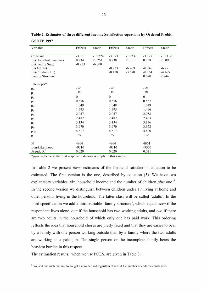
Table 2. Estimates of three different Income Satisfaction equations by Ordered Probit,

GSOEP 1997

Variable Effects t-ratio Effects t-ratio

Effects t-ratio

Constant -3.061 -10.224 -3.093 -10.232 -3.128 -10.319 Ln(Household income) 0.734 20.251 0.738 20.113 0.738 20.093 Ln(Family Size) -0.223 -6.800 Ln(Adults) -0.223 -6.269 -0.246 -6.751 Ln(Children + 1) -0.128 -3.680 -0.164 -4.465 Family Structure 0.070 2.844 Intercepts* µ0 - ∞ - ∞ - ∞ µ1 - ∞ - ∞ - ∞ µ2 0 0 0 µ3 0.556 0.556 0.557 µ4 1.049 1.048 1.049 µ5 1.495 1.495 1.496 µ6 2.057 2.057 2.058 µ7 2.482 2.482 2.483 µ8 3.134 3.134 3.136 µ9 3.970 3.970 3.972 µ10 4.617 4.617 4.620 µ11 + ∞ + ∞ + ∞ N 4964 4964 4964 Log-Likelihood -9310 -9310 -9306 Pseudo R2 0.020 0.020 0.021 *µ1=- ∞, because the first response category is empty in this sample.

In Table 2 we present three estimates of the financial satisfaction equation to be

estimated. The first version is the one, described by equation (5). We have two

explanatory variables, viz. household income and the number of children plus one 5.

In the second version we distinguish between children under 17 living at home and

other persons living in the household. The latter class will be called ‘adults’. In the

third specification we add a third variable ‘family structure’, which equals zero if the

respondent lives alone, one if the household has two working adults, and two if there

are two adults in the household of which only one has paid work. This ordering

reflects the idea that household chores are pretty fixed and that they are easier to bear

by a family with one person working outside than by a family where the two adults

are working in a paid job. The single person or the incomplete family bears the

heaviest burden in this respect.

The estimation results, when we use POLS, are given in Table 3.

5 We add one such that we do not get a non- defined logarithm of zero if the number of children equals zero.

27

Table 3. POLS results for the income satisfaction equations, GSOEP Variable Effects t-ratio effects t-ratio

Effects t-ratio

Constant -5.475 -19.849 -5.504 -19.663 -5.534 -19.770 Ln(Household income) 0.678 19.829 0.681 19.581 0.681 19.584 Ln(Family Size) -0.206 -6.624 Ln(Adults) -0.205 -6.122 -0.227 -6.597 Ln(Children + 1) -0.118 -3.645 -0.152 -4.407 Family Structure 0.065 2.842 N 4964 4964 4964 Adjusted R2 0.073 0.073 0.075

We see that the corresponding t- values are almost the same. The coefficients look

multiples of each other except for the constant.

The cardinal CP- or interval- regression approach yields the following estimates and

again we see that the ratios of coefficients are almost the same while the t-ratios

hardly differ.

Table 4. The Financial Satisfaction Question estimated by Cardinal Probit.

Variable Effects t-ratio effects t-ratio effects t-ratio

Constant -2.524 -18.236 -2.536 -18.055 -2.550 -18.159Ln(Household income) 0.342 19.923 0.343 19.652 0.343 19.657 Ln(Family Size) -0.102 -6.568 Ln(Adults) -0.101 -6.019 -0.112 -6.480 Ln(Children + 1) -0.060 -3.697 -0.076 -4.430 Family Structure 0.032 2.765

Sigma 0.466 94.190 0.466 94.190 0.465 94.184

N 4964 4964 4964 Log-Likelihood -9500 -9500 -9496 Pseudo R2 0.0198 0.0199 0.0202

28

Finally we use the COLS – approach with yields table (2.11) and again we see that the

ratios of coefficients and the t-ratios are almost the same.

Table 5. The Financial Satisfaction Question estimated by COLS Variable effects t-ratio effects t-ratio Effects t-ratio

Constant -2.464 -16.738 -2.477 -16.575 -2.492 -16.678 Ln(Household income) 0.354 19.388 0.355 19.123 0.355 19.126 Ln(Family Size) -0.108 -6.515 Ln(Adults) -0.107 -5.966 -0.118 -6.427 Ln(Children + 1) -0.063 -3.669 -0.081 -4.403 Family Structure 0.034 2.766

N 4964 4964 4964 Adjusted R2 0.070 0.070 0.072

The four methods used have the same objective, that is, the estimation of the equation

ln( ) ln( )Z y fsα β γ= + + ε+ (28)

where Z stands for a satisfaction index. The equation may be used for the derivation

of family equivalence scales6. If ln(fs) increases to ln(fs) + fs∆ , the question arises by

how much the individual has to be compensated in his income ln(y). We find

ln( ) ln( )y fsβα

∆ = − ∆ (29)

It follows that the indifference curves between income and family size are described by

0 0( / )y y fs fsβα

−= (30)

where and 0y 0fs stand for the reference income and reference family size,

respectively. Now it is interesting to see whether the ratio βα

is the same, irrespective

of the four methods used. We give the different values in Table 6.

6 See also Van Praag(1971),Van Praag and Kapteyn(1973).

29

Table 6. Equivalence scale parameter calculated via different methods.

method OP POLS CP COLS IEQ β/α 0.32 0.30 0.30 0.30 0.26

We see that the values of the ratio, estimated via four different methods, are virtually

identical. Actually, this is less surprising than it looks like, if we realize that this

equivalence scale describes an indifference curve, which is defined by the Financial

Satisfaction - question. Everybody who evaluates his income by the same number is

on the same indifference curve. The four methods yield different monotonic

transforms of satisfaction, but their ordinal information is the same. The fifth column,

derived from the IEQ, will be considered in a moment.

Let us now consider what is the relation between POLS and COLS - estimates.We

denote as before the ordinal variable, belonging to a specific response category, by

ln( ) and the corresponding cardinal value by ln( ). We assume ln( ) =f(ln( )).

As the categories are ordered , we may assume that f(.) is a monotonically increasing

function. Let us assume for a moment that both variables would be exactly measured

on a continuous scale instead of on a discrete scale, then the marginal distributions of

both variables would be normally distributed with parameters (

z z z

)

z

,µ σ and ( ),µ σ ,

respectively.

We may express a fraction of respondents to a specific category either with respect to

or with respect to . We have z z

(ln( ); , ) ( (ln( ); , )N z N f zµ σ µ σ≡ (31)

which implies

ln( ) (ln( ))z f zµ µσ σ

− −≡ (32)

It follows that the function f(.) is a linear affine transformation. We have

30

ln( ) ln( )z z Dσσ

= + (34)

where D is a constant which can be easily calculated. Indeed if we apply this

regression (on k observations) we find for the German data the regression result

ln( ) 0.5359ln( ) 0.1965Z Z= + .

with an R2 of 0.99.

It follows that, if l is a linear combination of variables x , then the same will

hold for l , where the trade - off ratios will be the same.

n( )z

n( )z

It follows that OP, POLS ,CP and COLS are for practical purposes equivalent for the

computations of trade - off ratios. The C- versions employ the cardinal part of the

information as well.

The implicit cardinalisation on which Probit and POLS are based will be called from

now on the frequentist cardinalisation because it is based on the frequency distribution

of satisfaction levels. The cardinalisation on which CP and COLS are based will be

called the satisfaction cardinalisation from now on. We notice that one is a linear

transformation of the other.

It is evident that we may also derive family equivalence scales from the IEQ. The

estimates of equation (23) are presented in Table 7.

Table 7. The IEQ – estimates for µ .

Variable Effects t-ratio Effects t-ratio effects t-ratio Constant 3.611 54.308 3.572 52.302 3.574 52.309 Ln(Household income) 0.527 61.964 0.533 60.667 0.533 60.644 Ln(Family Size) 0.121 14.819 Ln(Adults) 0.090 8.093 0.089 7.958 Ln(Children + 1) 0.096 11.976 0.083 5.355 Family Structure 0.011 0.963 σ 0.453 0.453 0.453 N 3962 3962 3962 Adjusted R2 0.631 0.632 0.632 It is obvious that we may derive for the individual welfare function household

equivalence scales by requiring that households with different family sizes fs0 and fs 1

31

enjoy an equal welfare level according to the true welfare function. This implies that

the indifference curve is described by

0.1210.473

0 0( / )y y fs fs= (35)

where the ratio β/α is replaced by β/(1-α). We notice that this power is 0.26. This

value is evidently very well in line with the other values in Table 6. Hence our

conclusion is that the ordinal information, which can be extracted from the true

welfare function is the same as that which is provided by the FS- question.

Obviously, we may also try to explain the six separate responses on the IEQ, that is

the household cost levels ln(ci). The resulting regression equations are given in table

8.

Table 8. Ordinal analysis of the six level equations of the IEQ.

C1 C2 C3 C4 C5 C6 Effect

s t-ratio Effect

s t-ratio Effect

s t-ratio Effect

s t-ratio Effect

s t-ratio effects t-ratio

i 3.499 33.653 3.422 42.488 3.447 46.647 3.558 51.176 3.788 51.033 3.961 41.326 i 0.468 35.134 0.507 49.193 0.527 55.774 0.539 60.572 0.550 57.904 0.571 46.534 βi 0.165 12.870 0.149 14.996 0.141 15.490 0.130 15.144 0.089 9.706 0.056 4.715 System Weighted R-Square: 0.2318 The errors are strongly correlated as we see from Table 9.

Table 9. The cross-model error correlation matrix.

C1 C2 C3 C4 C5 C6 C1 1 0.906 0.836 0.744 0.611 0.467 C2 0.906 1 0.963 0.887 0.784 0.630 C3 0.836 0.963 1 0.951 0.856 0.706 C4 0.744 0.887 0.951 1 0.917 0.772 C5 0.611 0.784 0.856 0.917 1 0.899 C6 0.467 0.630 0.706 0.772 0.899 1

For a more extensive ordinal analysis see Van Praag and Van der Sar (1988), where

similar results for other data sets were found. Our conclusion is that the coefficients

for the separate levels are not equal, but that they follow exactly the same pattern as in

Van Praag and Van der Sar. At a low level of satisfaction the dependency on own

32

income is considerable at 0.442, but it increases as the level of satisfaction increases

up to 0.593 at the highest level of satisfaction.

The family size effect β behaves just in the opposite way. It falls with rising levels of

satisfaction (see also (Van Praag, Flik (1992)) for a comparison with other European

data sets). We may stamp the effect of family size as reflecting real needs, while the

dependency on own income stands for a psychological reference effect. Our findings

may then be summarized as: when individuals become richer, their real needs become

less pressing and their norms become more determined by reference effects.

We may calculate for each verbal level i the income amount yi , which is evaluated by

i. For that level there holds

iiiii fsyy γβα ++= )ln()ln()ln( (i=1,…,6) (36)

which yields

i

iii

fsyα

γβ−

+=

1)ln()ln( (i=1,…,6) (37)

We notice that the resulting family size elasticity is βi /(1-i ). We notice that the

elasticities and the corresponding household equivalence scales hardly vary between

the satisfaction levels i.

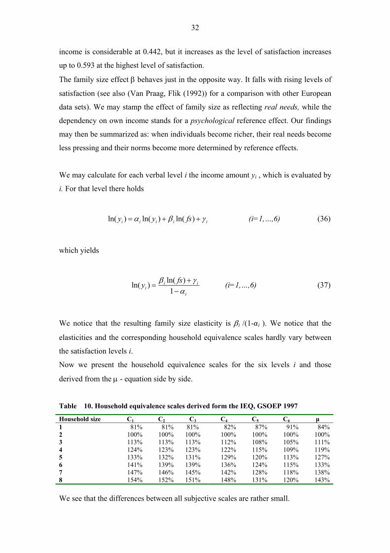
Now we present the household equivalence scales for the six levels i and those

derived from the µ - equation side by side.

Table 10. Household equivalence scales derived form the IEQ, GSOEP 1997

Household size C1 C2 C3 C4 C5 C6 µ 1 81% 81% 81% 82% 87% 91% 84% 2 100% 100% 100% 100% 100% 100% 100% 3 113% 113% 113% 112% 108% 105% 111% 4 124% 123% 123% 122% 115% 109% 119% 5 133% 132% 131% 129% 120% 113% 127% 6 141% 139% 139% 136% 124% 115% 133% 7 147% 146% 145% 142% 128% 118% 138% 8 154% 152% 151% 148% 131% 120% 143% We see that the differences between all subjective scales are rather small.

33

Van Praag and Flik (1992) derived equivalence scales for various European countries

by the same IEQ- method. They noticed that the scales in various countries are not the

same, reflecting cultural differences and differences in social systems. See also

Hagenaars (1986) and Goedhart et al. (1977).

Finally, it is interesting to compare the results derived from the IEQ- responses with

our results, based on Financial Satisfaction -responses. The resulting trade- offs,

derived from the true WFI, and the ratios found earlier are very similar. The

additional result that we can derive from the IEQ and which we cannot find from

financial satisfaction questions, because they only refer to current income, is the

virtual WFI. As said before the true WFI corresponds to the experienced utility

function and the virtual WFI to the decision utility function.

5. Conclusion Let us now summarise the conclusions of this paper.

• We found that income satisfaction can be explained by objective factors. This

yields trade - off coefficients between family size and income and trade- off

coefficients between adults and children.

• We found that the Ordered Probit - method is based on an implicit frequentist

utility assumption, which may be interpreted as a cardinalist approach as well.

• We saw that we may replace the O. Probit method by the method of Probit-

Adjusted Ordinary Least Squares (POLS) and that the results do not vary except for a

multiplication factor.

• We found that we can use the cardinal information in Financial Satisfaction

Questions leading to a Cardinal Probit - and a Cardinal OLS - approach.

• The frequentist and the cardinalist approach imply two different

cardinalisations of satisfaction, which are related by an affine linear transformation.

34

• The empirical estimates according to those four estimation methods are

strongly related and yield (almost) the same trade - off - ratios.

• The POLS - and COLS methods are computationally easier.

• An earlier way to study income satisfaction in a quantitative way has been

developed by Van Praag and Kapteyn ('Leyden School'). In this chapter we compare

their results derived from the Income Evaluation Question with results derived from

the Financial Satisfaction Question (FSQ). We found that both methods yield

approximately the same trade - off coefficients.

• The FSQ yields an experienced utility function in the terms of Kahneman et al.

The IEQ yields a virtual and a true individual welfare function, which concepts

coincide with Kahneman et al.'s decision utility and experienced utility functions,

respectively. The result of this comparison is that most results derived by WFI-

analysis by or in the spirit of the 'Leyden School' could have been derived by analysis

of the FSQ as well.

• The FSQ is easier to answer for to respondents than the IEQ. Moreover, the

IEQ - format does not seem applicable when we ask for Health Satisfaction, Housing

Satisfaction, etc., while the FSQ can be used. However, the IEQ yields information on

the decision utility function, which the FSQ cannot provide.

References

Brickman, P. and Campbell, D.T., 1971. Hedonic relativism and planning the good

society. In: Apley, M.H., (Ed.), Adaptation-level theory: A symposium, Academic

Press: NY. pp. 287-302.

Clark, A. E. and Oswald, A. J., 1994. 'Unhappiness and unemployment'. Economic

Journal, 104: 648-659.

Cramèr, H., 1937, Random Variables and Probability Distributions, Cambridge tracts

in Mathematics and Math. Physics 36, Cambridge University Press,

Cambridge(U.K.).

Edgeworth, F.Y., [1881], 1961, Mathematical Psychics, A.M. Kelley, N.Y.

Easterlin, R. A. (1974). ‘Does Economic growth improve the human lot? Some

empirical evidence’. In P.A. David and M.W. Reder (eds.), Nations and

35

Households in Economic Growth. Essays in Honor of Moses Abramowitz. New

York, Academic Press, 89-125.

Easterlin, R. A. (1995). ‘Will Raising the Incomes of All Increase the Happiness of

All?’ Journal of Economic Behavior and Organization, 27 (1): 35-47.

Easterlin, R.A. (2001). ‘Income and Happiness: Towards a unified Theory’. Economic

Journal, 111: 465-84.

Feller ,W. 1971, An Introduction to Probability Theory and Its Applications, Volume

2, Wiley & Son, New York

Ferrer-i-Carbonell, A. and Van Praag, B.M.S., 2001. Poverty in Russia. Journal of

Happiness Studies, 2: 147-172.

Ferrer-i-Carbonell, A. and B.M.S. van Praag, 2002. The subjective costs of health

losses due to chronic diseases. An alternative model for monetary appraisal. Health

Economics, 11: 709-722.

Frisch, R. 1959.Dynamic Utility. Econometrica,32,p.418-29.

Goedhart, Th., Halberstadt, V., Kapteyn, A. and van Praag, B.M.S., 1977. The

poverty line: concept and measurement. Journal of Human Resources, 12: 503-

520.

Greene, W.H., 1991. Econometric Analysis. MacMillan Publishing Company, New

York.

Greene, W., 2005. 'Censored Data and Truncated Distributions', forthcoming in The

Handbook of Econometrics:Vol.1, ed. T.Mills and K.Patterson, Palgrave, London.

Hagenaars, A.J.M., 1986. The perception of poverty. North-Holland Publish

Company, Amsterdam.

Hicks, J.R., 1939. The foundations of welfare economics. Economic Journal, 49:

696-712.

Houthakker,H.S.,1950. Revealed preference and the utility function'.

Economica,17,p.159-74.

Kahneman, D., P.P. Wakker and R. Sarin, 1997. Back to Bentham? Explorations of

experienced utility. Quarterly Journal of Economics, 2: 375-405.

Pareto,V.,1909. Manuel d’économie politique.Paris, Giard et Brière.

Plug ,E.J.S., P. Krause, B.M.S. van Praag, G.G. Wagner Measurement of

Poverty:Examplified by the German Case. In: Income Inequality and Poverty in

Eastern and Western Europe.1997 .Heidelberg, Phusica-Verlag, pp. 69-89

36

Rao,C.R.,1973, Linear Statistical Inference and Its Applications, Wiley &Sons, New

York.

Robbins, L., 1932. An Essay on the Nature and Significance of Economic Science.

MacMillan, London.Rowntree, B.S., 1941. Poverty and progress, Longmans ,

Green and Co, London.

Ronning, G; M Kukuk (1996), 'Efficient Estimation of Ordered Probit Models'.

Journal of the American Statistical Association, Vol. 91, No. 435., pp. 1120-

1129.

Stewart, M. (1983). ‘On least squares estimation when the dependent variable is

grouped’. Review of Economic Studies, 50: 141-49.

Terza, J. V. (1987) ‘Estimating linear models with ordinal qualitative regressors’.

Journal of Econometrics, 34(3): 275-91.

Samuelson, P.A., 1947. Foundations of Economic Analysis. Harvard U.P.,

Cambridge, Massachusetts.

Seidl, C., 1994. How Sensible is the Leyden Individual Welfare Function of Income?

in: European Economic Review, Vol. 38/8: 1633 - 1659.

Suppes, P. and M. Winet, 1954. An Axiomatization of Utility Based on the Notion of

Utility Differences. Management Science, 1: 259-70.

Van Praag, B.M.S., 1968. Individual welfare functions and consumer behavior. A

theory of rational irrationality. Ph.D. Thesis, North Holland Publishing Company,

Amsterdam.

Van Praag, Bernard M.S. and Kapteyn, A., 1973. Further evidence on the individual

welfare function of income: an empirical investigation in the Netherlands.

European Economic Review. 4:33-62.

Van Praag B.M.S., 1971. The welfare function of income in Belgium: an empirical

investigation. European Economic Review, 2: 337-369

Van Praag, B.M.S. and van der Sar, N.L., 1988. Household cost functions and

equivalence scales. Journal of Human Resources. 23: 193-210.

Praag, van B.M.S., 1991. Ordinal and cardinal utility: an integration of the two

dimensions of the welfare concept. Journal of Econometrics, 50: 69-89.

Praag, van B.M.S., 1994. Ordinal and cardinal utility: an integration of the two

dimensions of the welfare concept. Revision of (1991) in R.F.Blundell,

37

I.Preston,I.Walker (eds.) The measurement of household welfare, Cambridge

University Press.

Van Praag, B.M.S. and Flik, R.J.,1992. Poverty lines and equivalence scales. A

theoretical and empirical investigation. In Poverty Measurement for Economies

in Transition in Eastern Europe, International Scientific Conference, Warsaw,

7-9 October, Polish Statistical Association, Central Statistical Office.

van Praag, B.M.S., Frijters, P., and Ferrer-i-Carbonell, A., 2003. 'The anatomy of

subjective well-being', Journal of Economic Behavior and Organization, 51(1): 29-

49.

Van Praag,B.M.S. and A. Ferrer-i-Carbonell (2004), Happiness Quantified, A

Satisfaction Calculus Approach. Oxford University Press.

Van Praag, B.M.S. and A. Ferrer-i-Carbonell (2006), 'An Almost Integration-free

Approach to Ordered Response Models', working paper, Tinbergen Institute.