The Consecutive Multiprocessor Job Scheduling Problem

Yossi Bukchin1

Department of Industrial Engineering,

Tel-Aviv University, Ramat Aviv 6997801, Tel Aviv, Israel

Email: bukchin@tau.ac.il

Tal Raviv

Department of Industrial Engineering,

Tel-Aviv University, Ramat Aviv 6997801, Tel Aviv, Israel

Email: talraviv@eng.tau.ac.il

Ilya Zaides

Department of Industrial Engineering,

Tel-Aviv University, Ramat Aviv 6997801, Tel Aviv, Israel

Email: ilyazaides@mail.tau.ac.il

Submitted: September 2018

Revised: May 2019

1 Corresponding author

2

The Consecutive Multiprocessor Job Scheduling Problem

Abstract

We study a variant of the multiprocessor job scheduling problem, where jobs are

processed by several identical machines. The machines are ordered in a sequence,

and each job is processed by several consecutive machines simultaneously. The

jobs are characterized by their processing time, the number of required consecutive

machines, and their ready time. The objective function is to minimize the sum of

general functions defined over the completion time of each job. This study is

motivated by a real problem in the semiconductor industry. We present a time-

indexed integer programming and a constraint programming formulations for the

problem and demonstrate their applicability through an extensive numerical study

and an industrial case study.

Keywords: multiprocessor job scheduling, integer programming, constraint

programming

1. Introduction and preliminaries

We study a scheduling problem that can be stated as follows: A system with an

ordered set of 𝑚 identical machines, located one next to the other, is used to process a

set of 𝑛 jobs. The processing of each job occupies a set of several consecutive machines

simultaneously, while each machine can process at most one job at a time. Each job is

characterized by its processing time, number of required consecutive machines, ready

time, and, possibly, due date. For example, a job that requires three machines, with a

time duration of five hours, may be processed simultaneously on machines 2, 3 and 4,

starting at 𝑡 = 7 and ending at 𝑡 = 12. The objective function is to minimize the sum

of general functions defined over the completion time of each job. This includes

minimizing the number of tardy jobs, and minimizing the total tardiness, as special

cases. The problem is named the Consecutive Multiprocessor Job Scheduling Problem.

It is a generalization of some known NP-hard and inapproximable scheduling problems,

including minimizing the number of tardy jobs on parallel machines, see for example

(Pinedo, 2012).

This study is motivated by a real-world application of allocating computing

resources during the development of new integrated circuits in the semiconductors

industry. The computing resources are hardware emulators that are being used to save

3

time and costs associated with the verification of new designs before beginning the

manufacturing process. Each verification job needs to be processed by several

consecutive emulators in the array for a given time. The developers in the various

departments specify in advance the time by which each design will be ready for

verification. The due dates are dictated by the production plans of the FABs and other

managerial considerations. The emulators are expensive and scarce. Thus, it is

important to utilize them efficiently. Similar problems arise in different applications,

such as allocating berth space and cranes in a seaport.

In this study, we present two formulations for the consecutive multiprocessor job

scheduling problem: a time-indexed integer programming (IP) model and a constraint

programming (CP) model. In an extensive numerical study, we compare these

formulations with state-of-the-art formulations from the literature and demonstrate their

effectiveness. Our time-indexed formulation can be viewed as a generalization of

previous similar formulations for classic parallel machine scheduling problems, see for

example (Sevaux & Thomin, 2001). In addition, we apply our method in a rolling

horizon scheme for an Industrial case study and compare its performance with the

current practice.

The rest of this paper is organized as follows. In Section 2, we review the current

literature and identify the gaps that need to be addressed. In Section 3, we the

formulations for the consecutive multiprocessor job scheduling problem. The

performance of these formulations are tested with commercial solvers in Section 4, and

are compared with a previous formulation that is capable of solving some special cases

of the problem. In Section 5, we present the results of an industrial case study where

our algorithm is applied in a dynamic setting. Concluding remarks are given in Section

6.

2. Literature review

The problem of scheduling jobs on multiple processors shares similar properties to

well-studied problems such as scheduling jobs on parallel machines, the multiprocessor

scheduling problem, strip packing and cutting problems, the berth allocation problem

(BAP); however, the studied problem differs from the ones discussed in the literature

either by the scheduling environment or by the objective function.

4

(Leonardi & Raz, 2007) studied the parallel processors for minimizing total flow

time problem (known as 𝑃/𝑟𝑖/∑ 𝑐𝑖). They proved that the problem is not approximable

within 𝑂 (𝑛1

3−𝜖) for any 𝜖 > 0. This problem is a special case of our problem since we

consider jobs that require more than one machine at a time. We conclude that the

Consecutive Multiprocessor Job Scheduling Problem is strongly NP-hard and is not

approximable within a constant. Hence, the motivation for the solution methods

presented in this paper.

The general multiprocessor job scheduling has been studied in (Bianco,

Blazewicz, Dell'Olmo, & Drozdowski, 1995) and (Chen & Lee, 1999). In the

generalized problem, each job can be processed by multiple alternative sets of

machines, not necessarily with identical cardinality. For example, job 𝑖 can be

processed either by machines {2, 4} or by machines {3, 4, 5}. Hence, all alternatives

have to be explicitly presented. In (Chen & Lee, 1999), a two phase heuristic is

proposed for solving the problem of a general multiprocessor with the objective of

minimizing the makespan, as follows: an assignment phase, in which alternatives are

being chosen for each job, and a scheduling phase, in which the job ordering is being

determined. (Baptiste, 2003) addresses a special case of the general multiprocessors

scheduling problem, when all jobs have the same processing time and each job has its

own ready time and size (required number of machines). He shows that both completion

time and makespan minimization problems can be solved in polynomial time using a

dynamic programming algorithm. (Huang, Chen, & Wang, 2007) present a linear time

1.5 approximation algorithm for minimizing the makespan on four machines.

Note that in our model, each job has its own size, which is the required number

of consecutive machines, and hence, the problem can be expressed in a more concise

manner. Cutting rectangular elements and strip packing problems, see for example,

(Martello, Monaci, & Vigo, 2003) have similar structure to our problem but differ in

their objective function, constraints and in the fact that the size of each job is not

necessarily discrete.

Some variations of the berth allocation problem (BAP) are highly related to the

general multiprocessor scheduling problems. This problem deals with allocating berth

space and cranes in seaports to arriving vessels that have to be loaded and unloaded. As

5

described in (Bierwirth & Meisel, 2010), there are three variations of this problem, as

follows:

1. Discrete case (BAP-D). The quay is divided into separate sections, where each

section (berth) can serve one vessel at a time (Imai, Chia, Etsuko, & Papadimitriou,

2008), (Imai, Nishimura, & Papadimitriou, 2001).

2. Continuous case (BAP-C). In this case, a vessel can berth anywhere along the quay.

Consequently, the quay can serve a number of vessels simultaneously (Park & Kim,

2005) (Imai, Sun, Nishimura, & Papadimitriou, 2005).

3. Hybrid case (BAP-H). The quay is divided into separate sections, as each section is

continuous and may serve several vessels, and each vessel may occupy several

sections (Umang, Bierlaire, & Vacca, 2013).

The first case (BAP-D) is analogous to the classic parallel machine problem, as

each vessel\job can be served by a single section (machine). The second case, (BAP-C)

is analogous to our problem, if the size of the vessels (jobs) and the length of the quay

(sequence of machines) are integers. Our problem is also a special case of the third case

(BAP-H), where no two vessels are small enough to fit into one quay section.

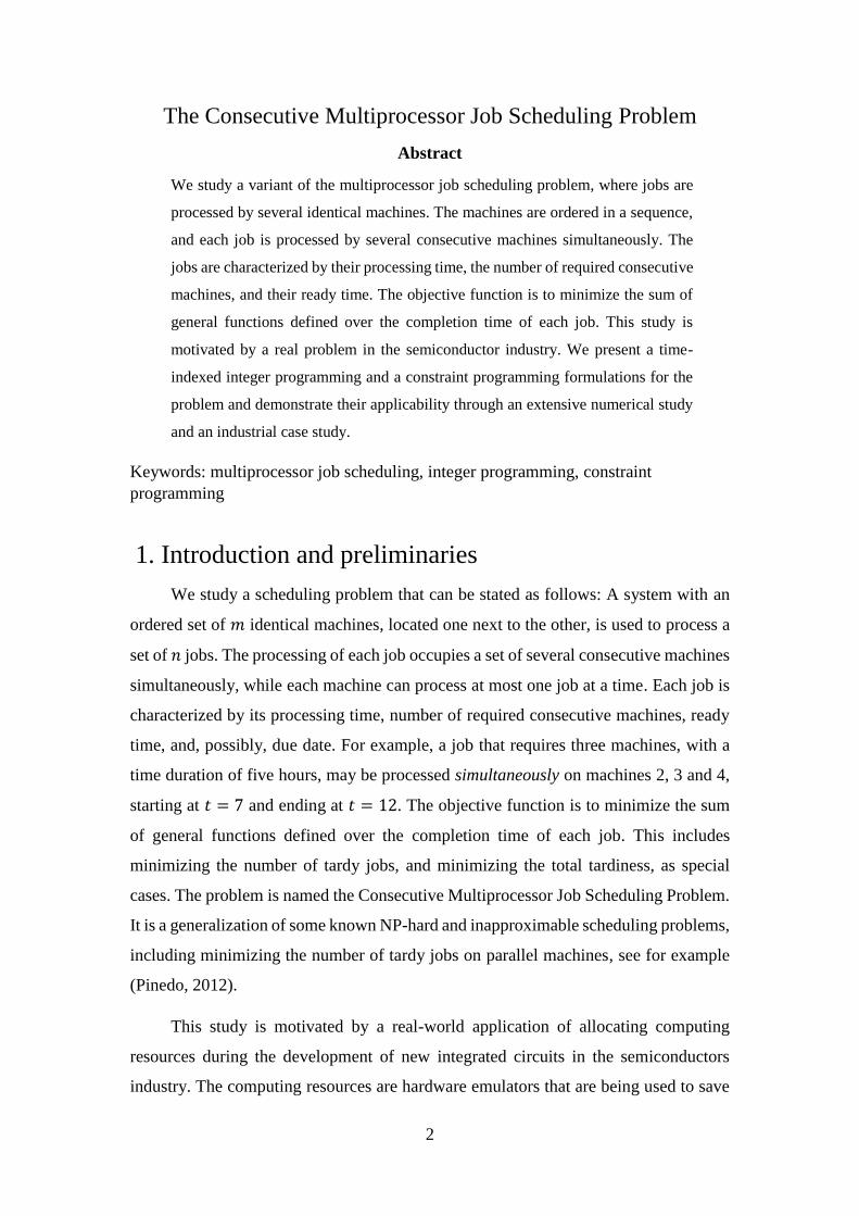
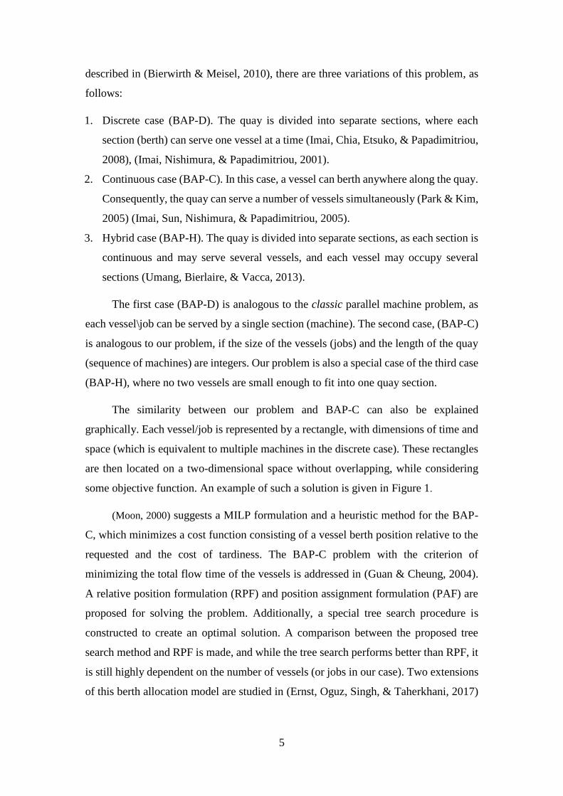
The similarity between our problem and BAP-C can also be explained

graphically. Each vessel/job is represented by a rectangle, with dimensions of time and

space (which is equivalent to multiple machines in the discrete case). These rectangles

are then located on a two-dimensional space without overlapping, while considering

some objective function. An example of such a solution is given in Figure 1.

(Moon, 2000) suggests a MILP formulation and a heuristic method for the BAP-

C, which minimizes a cost function consisting of a vessel berth position relative to the

requested and the cost of tardiness. The BAP-C problem with the criterion of

minimizing the total flow time of the vessels is addressed in (Guan & Cheung, 2004).

A relative position formulation (RPF) and position assignment formulation (PAF) are

proposed for solving the problem. Additionally, a special tree search procedure is

constructed to create an optimal solution. A comparison between the proposed tree

search method and RPF is made, and while the tree search performs better than RPF, it

is still highly dependent on the number of vessels (or jobs in our case). Two extensions

of this berth allocation model are studied in (Ernst, Oguz, Singh, & Taherkhani, 2017)

6

and (Agra & Oliveira, 2018). The former considers high tide and the latter combines

the crane assignment to vessels.

5

4

3 Vessel\Job 3

2

1

1 2 3 4 5 6 7 8 9 10 11

Ber

th /

Mac

hin

e

Time

Vessel\Job 2

Vessel\Job 1

Vessel\Job 5

Vessel\Job 4

Figure 1. Schedule example

The contribution of our study with respect to the state of the art of the equivalent

BAP-C problem is as follows. First, we present new integer programming (IP) and

constraint programming (CP) models, which perform well compared to the current

existing formulation of (Guan & Cheung, 2004), when solved with a commercial solver

(CPLEX in our case). Second, our model is more general in the objective function, as

it is capable of optimizing any objective function that is separable in the completion

time of the jobs, including nonlinear functions. Such objective functions may be found

in various applications in both the contexts of machine and berth scheduling. For

example, when the processing costs vary over the hours of the day due to time-of-use

electricity tariffs or different labor costs at various hours of the day/week. Finally, we

implement our model in a rolling horizon setting to simulate scheduling of test jobs on

hardware emulators. Our simulation is based on real-life datasets obtained from a major

semiconductor company. We show that our algorithm performs well for this real-world

problem, and significantly outperforms the current policy.

3. Mathematical formulations

In this section, we present a time-indexed integer programming formulation and a

constraint programming formulation for the consecutive multiprocessor job scheduling

problem. In addition, a benchmark mixed integer formulation, inspired by the model of

(Guan & Cheung, 2004), was developed and is presented in Appendix A. For each of

7

our modeling techniques, we start with an important special case, which is the

minimization of the number of tardy jobs and continue to the general objective function

that captures many well-studied scheduling problems with general ready times and due

dates. Both objectives were inspired by the real-world case study, mentioned above.

Let us first introduce some notation for the parameters of the problem.

𝑛 number of jobs

𝑚 number of machines

𝑝𝑖 processing time of job 𝑖 = 1,… , 𝑛

𝑠𝑖 number of consecutive machines required for the processing of job 𝑖 (aka

size of job 𝑖) 𝑟𝑖 ready time of job 𝑖, note that since the time periods are discrete and

indexed from 1, 𝑟𝑖 = 𝑡 implies that the earliest period on which the jobs

can start is 𝑡 + 1.

𝑑𝑖 due date of job 𝑖 𝑇 the length of the planning horizon.

Throughout the paper, we assume that all the numerical parameters are integers. Based

on this assumption, one can assume, without loss of generality, that the starting and

completion times of the job are all integers. The planning horizon is divided into 𝑇

discrete periods where Job 𝑖 becomes available at the end of period 𝑟𝑖 and is due by the

end of period 𝑑𝑖.

3.1. Time-indexed integer programming formulation

We first introduce a time-indexed integer programming formulation, which minimizes

the number of tardy jobs. To this end, we define the following decision variable:

𝑥𝑖𝑗𝑡 A binary decision variable that equals one if job 𝑖 is scheduled to start on

machines 𝑗, … , 𝑗 + 𝑠1 − 1 at time 𝑡. Both the periods and the machines are

indexed from one.

For the sake of compact presentation of the model we define the following parameters:

𝛼𝑖𝑗 The lowest starting machine index possible for job 𝑖 given it occupies

machine 𝑗. 𝛼𝑖𝑗 = 𝑚𝑎𝑥{1, 𝑗 − 𝑠𝑖 + 1}.

𝛽𝑖𝑡 The earliest starting period for job 𝑖 given it is still being processed at

period 𝑡. 𝛽𝑖𝑡 = 𝑚𝑎𝑥{𝑟𝑖 + 1, 𝑡 − 𝑝𝑖+ 1}

𝛾𝑖𝑡 The latest starting period for job 𝑖 given that it is still being processed at

period 𝑡. 𝛾𝑖𝑡 = min{𝑑𝑖 − 𝑝𝑖+ 1, 𝑡}

8

Model IP-U

max {∑ ∑ ∑ 𝑥𝑖𝑗𝑡

𝑑𝑖−𝑝𝑖+1

𝑡=𝑟𝑖+1

𝑚−𝑠𝑖+1

𝑗=1

𝑛

𝑖=1

}

(1)

Subject to:

∑ ∑ 𝑥𝑖𝑗𝑡 ≤ 1

𝑑𝑖−𝑝𝑖+1

𝑡=𝑟𝑖+1

𝑚−𝑠𝑖+1

𝑗=1

𝑖 = 1, . . . , 𝑛

(2)

∑ ∑ ∑ 𝑥𝑖𝑗′𝑡′ ≤ 1

𝛾𝑖𝑡

𝑡′=𝛽𝑖𝑡

𝑗

𝑗′=𝛼𝑖𝑗

𝑛

𝑖=1

𝑗 = 1, . . . , 𝑚

𝑡 = 1,… ,max𝑖

𝑑𝑖 (3)

𝑥𝑖𝑗𝑡 ∈ {0,1} 𝑖 = 1, . . . , 𝑛

𝑗 = 1, . . . , 𝑚 − 𝑠𝑖 + 1, 𝑡 = 𝑟𝑖 + 1,… , 𝑑𝑖 − 𝑝𝑖 + 1

(4)

The objective function (1) maximizes the total number of jobs that were completed

before their due date. This objective is equivalent to minimizing the number of tardy

jobs. Constraint (2) assures that each job is processed at most once; no scheduling

decisions are made for jobs that cannot meet their due date. Constraint (3) is a non-

overlapping constraint, which eliminates the possibility of scheduling multiple jobs on

the same machine at the same time. Note that only assignments of jobs to feasible

machines and starting times that cover machine 𝑗 at times 𝑡 are summed at the left-hand

side. Indeed, if 𝑡 > 𝑑𝑖 or 𝑡 < 𝑟𝑖 then 𝛽𝑖𝑡 > 𝛾𝑖𝑡. In such case the summation is empty.

In (4), the binary decision variables are defined for all possible starting periods of jobs

within their allowed period.

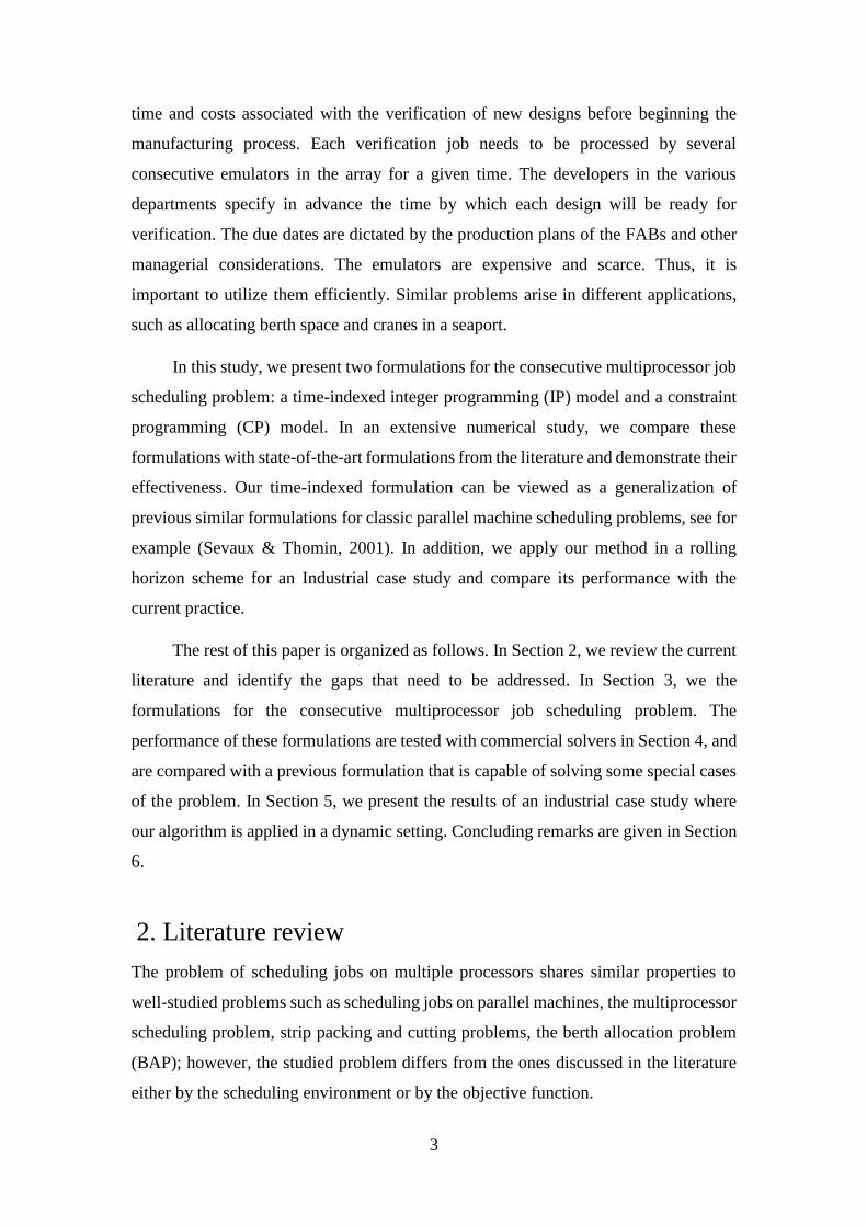
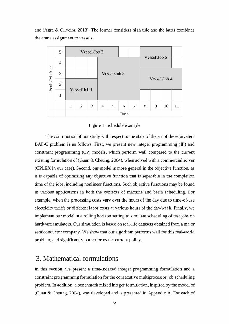
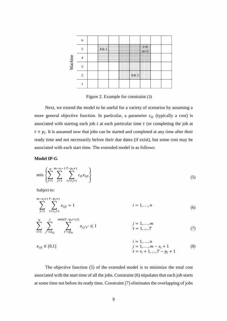
A toy example, to demonstrate the non-overlapping constraint (3), is given in

Figure 2. Assume that only two jobs are considered, job 1, with 𝑝1 = 5, and 𝑠1 = 2,

and job 2, with 𝑝2 = 3, and 𝑠2 = 4. Let us consider the overlapping avoidance at 𝑡 =

6, 𝑗 = 5. In this case, job 1 will use machine 5 in time 6 only when 𝑥1𝑗𝑡 = 1 for any

combination of 𝑗 ∈ {4, 5}, and 𝑡 ∈ {2,… ,6}. Similarly, job 2 will use the same slot

(machine 5 in time 6) only when 𝑥2𝑗𝑡 = 1 for any combination of 𝑗 ∈ {2, … ,5}, and 𝑡 ∈

{4,… ,6}. Constraint (3) then sums over these ranges for the 𝑥 variables of the two jobs,

bounding the summation by 1, i.e., ∑ ∑ 𝑥1𝑘𝑡′6𝑡′=2

5𝑘=4 + ∑ ∑ 𝑥2𝑘𝑡′

6𝑡′=4

5𝑘=2 ≤ 1.

9

6

5 Job 1t=6

m=5

4

3

2 Job 2

1

Mac

hin

e

Figure 2. Example for constraint (3)

Next, we extend the model to be useful for a variety of scenarios by assuming a

more general objective function. In particular, a parameter 𝑐𝑖𝑡 (typically a cost) is

associated with starting each job 𝑖 at each particular time 𝑡 (or completing the job at

𝑡 + 𝑝𝑖. It is assumed now that jobs can be started and completed at any time after their

ready time and not necessarily before their due dates (if exist), but some cost may be

associated with each start time. The extended model is as follows:

Model IP-G

min {∑ ∑ ∑ 𝑐𝑖𝑡𝑥𝑖𝑗𝑡

𝑇−𝑝𝑖+1

𝑡=𝑟𝑖+1

𝑚−𝑠𝑖−1

𝑗=1

𝑛

𝑖=1

}

(5)

Subject to:

∑ ∑ 𝑥𝑖𝑗𝑡 = 1

𝑇−𝑝𝑖+1

𝑡=𝑟𝑖+1

𝑚−𝑠𝑖+1

𝑗=1

𝑖 = 1, . . . , 𝑛

(6)

∑ ∑ ∑ 𝑥𝑖𝑗′𝑡′ ≤ 1

min{𝑇−𝑝𝑖+1,𝑡}

𝑡′=𝛽𝑖𝑡

𝑗

𝑗′=𝛼𝑖𝑗

𝑛

𝑖=1

𝑗 = 1, . . . , 𝑚

𝑡 = 1,… , 𝑇

(7)

𝑥𝑖𝑗𝑡 ∈ {0,1} 𝑖 = 1, . . . , 𝑛

𝑗 = 1, . . . , 𝑚 − 𝑠𝑖 + 1

𝑡 = 𝑟𝑖 + 1,… , 𝑇 − 𝑝𝑖 + 1

(8)

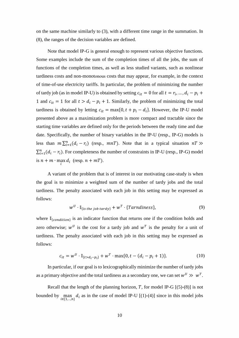
The objective function (5) of the extended model is to minimize the total cost

associated with the start time of all the jobs. Constraint (6) stipulates that each job starts

at some time not before its ready time. Constraint (7) eliminates the overlapping of jobs

10

on the same machine similarly to (3), with a different time range in the summation. In

(8), the ranges of the decision variables are defined.

Note that model IP-G is general enough to represent various objective functions.

Some examples include the sum of the completion times of all the jobs, the sum of

functions of the completion times, as well as less studied variants, such as nonlinear

tardiness costs and non-monotonous costs that may appear, for example, in the context

of time-of-use electricity tariffs. In particular, the problem of minimizing the number

of tardy job (as in model IP-U) is obtained by setting 𝑐𝑖𝑡 = 0 for all 𝑡 = 𝑟𝑖, … , 𝑑𝑖 − 𝑝𝑖 +

1 and 𝑐𝑖𝑡 = 1 for all 𝑡 > 𝑑𝑖 − 𝑝𝑖 + 1. Similarly, the problem of minimizing the total

tardiness is obtained by letting 𝑐𝑖𝑡 = max{0, 𝑡 + 𝑝𝑖 − 𝑑𝑖}. However, the IP-U model

presented above as a maximization problem is more compact and tractable since the

starting time variables are defined only for the periods between the ready time and due

date. Specifically, the number of binary variables in the IP-U (resp., IP-G) models is

less than 𝑚∑ (𝑑𝑖 − 𝑟𝑖)𝑛𝑖=1 (resp., 𝑚𝑛𝑇). Note that in a typical situation 𝑛𝑇 ≫

∑ (𝑑𝑖 − 𝑟𝑖)𝑛𝑖=1 . For completeness the number of constraints in IP-U (resp., IP-G) model

is 𝑛 +𝑚 ∙ max𝑖

𝑑𝑖 (resp. 𝑛 +𝑚𝑇).

A variant of the problem that is of interest in our motivating case-study is when

the goal is to minimize a weighted sum of the number of tardy jobs and the total

tardiness. The penalty associated with each job in this setting may be expressed as

follows:

𝑤𝑈 ⋅ 𝕀{𝑖𝑠𝑡ℎ𝑒𝑗𝑜𝑏𝑡𝑎𝑟𝑑𝑦} + 𝑤𝑇 ⋅ {𝑇𝑎𝑟𝑛𝑑𝑖𝑛𝑒𝑠𝑠}, (9)

where 𝕀{𝑐𝑜𝑛𝑑𝑖𝑡𝑖𝑜𝑛} is an indicator function that returns one if the condition holds and

zero otherwise; 𝑤𝑈 is the cost for a tardy job and 𝑤𝑇 is the penalty for a unit of

tardiness. The penalty associated with each job in this setting may be expressed as

follows:

𝑐𝑖𝑡 = 𝑤𝑈 ⋅ 𝕀{𝑡>𝑑𝑖−𝑝𝑖} + 𝑤𝑇 ⋅ max{0, 𝑡 − (𝑑𝑖 − 𝑝𝑖 + 1)}. (10)

In particular, if our goal is to lexicographically minimize the number of tardy jobs

as a primary objective and the total tardiness as a secondary one, we can set 𝑤𝑈 ≫𝑤𝑇.

Recall that the length of the planning horizon, 𝑇, for model IP-G [(5)-(8)] is not

bounded by max𝑖∈{1,…,𝑛}

𝑑𝑖 as in the case of model IP-U [(1)-(4)] since in this model jobs

11

can be scheduled to be completed after their due date. The value of 𝑇 dictates the

number of decision variables and hence the tractability of the model. If 𝑇 is externally

given, the model does not necessarily admit a feasible solution. In case 𝑇 is to be

determined internally, and the cost associated with the completion time is non-

decreasing over time, an upper bound of 𝑇 in an optimal solution is given by the

following:

𝑇′ = max𝑖∈{1,…,𝑛}

𝑟𝑖 +∑𝑝𝑖

𝑛

𝑖=1

. (11)

The upper bound, 𝑇′, is valid because any schedule that is ended after it must

contain periods in which all the machine are idle and all the remaining jobs are ready.

If the objective function is non-decreasing in the completion time of all the jobs, it is

always possible to shift the jobs that are scheduled after the idle period to an earlier

time without increasing the value of the objective function.

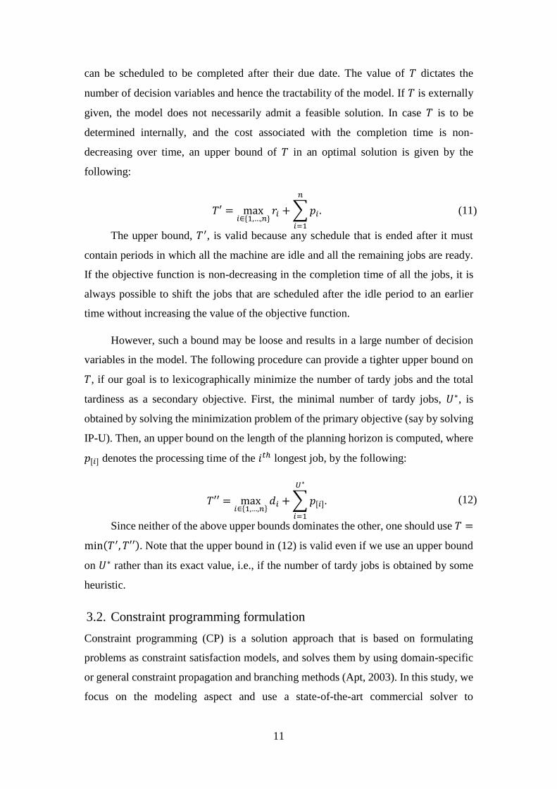
However, such a bound may be loose and results in a large number of decision

variables in the model. The following procedure can provide a tighter upper bound on

𝑇, if our goal is to lexicographically minimize the number of tardy jobs and the total

tardiness as a secondary objective. First, the minimal number of tardy jobs, 𝑈∗, is

obtained by solving the minimization problem of the primary objective (say by solving

IP-U). Then, an upper bound on the length of the planning horizon is computed, where

𝑝[𝑖] denotes the processing time of the 𝑖𝑡ℎ longest job, by the following:

𝑇′′ = max𝑖∈{1,…,𝑛}

𝑑𝑖 +∑𝑝[𝑖]

𝑈∗

𝑖=1

. (12)

Since neither of the above upper bounds dominates the other, one should use 𝑇 =

min(𝑇′, 𝑇′′). Note that the upper bound in (12) is valid even if we use an upper bound

on 𝑈∗ rather than its exact value, i.e., if the number of tardy jobs is obtained by some

heuristic.

3.2. Constraint programming formulation

Constraint programming (CP) is a solution approach that is based on formulating

problems as constraint satisfaction models, and solves them by using domain-specific

or general constraint propagation and branching methods (Apt, 2003). In this study, we

focus on the modeling aspect and use a state-of-the-art commercial solver to

12

demonstrate the effectiveness of our formulation. Using a general solver (either

commercial or open source) is a practical and attractive option because it enables very

rapid implementation of solution methods for a diverse set of optimization problems.

CP has been successfully used to solve a variety of problems in the domains of

vehicle routing, scheduling, timetabling and others. See, for example, (Shaw, 1998),

(Baptiste, 2003) and (Bukchin & Raviv, 2018). A CP model resembles an IP model in

terms of syntax. It contains a declaration of decision variables with their domains, a set

of constraints, and possibly an objective function. However, the CP modeling paradigm

is much more expressive. In fact, the language is a superset of the integer linear

programming modeling language. In addition to equality and inequality constraints

between linear mathematical expressions, a CP model can contain nonlinear

expressions, logical expressions, use decision variables as indices to other vectors of

decision variables, and can include global constraints that capture a relationship

between large sets of decision variables. There is no agreeable syntax for describing a

CP model, and each solver implements a different modeling language that is suitable to

express the type of constraint that it can propagate. Here, we are using the syntax

inspired by the OPL language used by the ILOG CP Solver, a commercial package that

we used for our numerical experiments. Some CP modeling constructs, used in our CP

formulations below, are demonstrated in Appendix B.

Next, we present our CP model. As with the IP formulation, we will start with a

model that minimizes the number of tardy jobs, which is equivalent to IP-U, and

continue with a more general model that can optimize an arbitrary function over the

completion times of the jobs. To this end, we introduce two sets of interval decision

variables.

𝐽𝑖 Represents the scheduled time of job 𝑖 - this is an optional interval with a

predefined duration, minimal start time and maximal end time.

𝐴𝑖𝑗 An auxiliary optional interval variable that is used to prevent jobs from

overlapping on machines.

13

Model CP-U

max∑presenceOf(𝐽𝑖)

𝑛

𝑖=1

(13)

Subject to:

altenative(𝐽𝑖, {𝐴𝑖1, … , 𝐴𝑖,𝑚−𝑠𝑖+1}) 𝑖 = 1, … , 𝑛 (14)

∑ ∑ pulse(𝐴𝑖𝑘, 1)𝑗𝑘=max(1,𝑗−𝑠𝑖+1)

𝑛𝑖=1 ≤ 1 𝑗 = 1,… ,𝑚 (15)

𝐽𝑖 interval, optional, length 𝑝𝑖 in 𝑟𝑖, …𝑑𝑖 𝑖 = 1, … , 𝑛 (16)

𝐴𝑖𝑗 interval, optional 𝑖 = 1, … , 𝑛,

𝑗 = 1,… ,𝑚 (17)

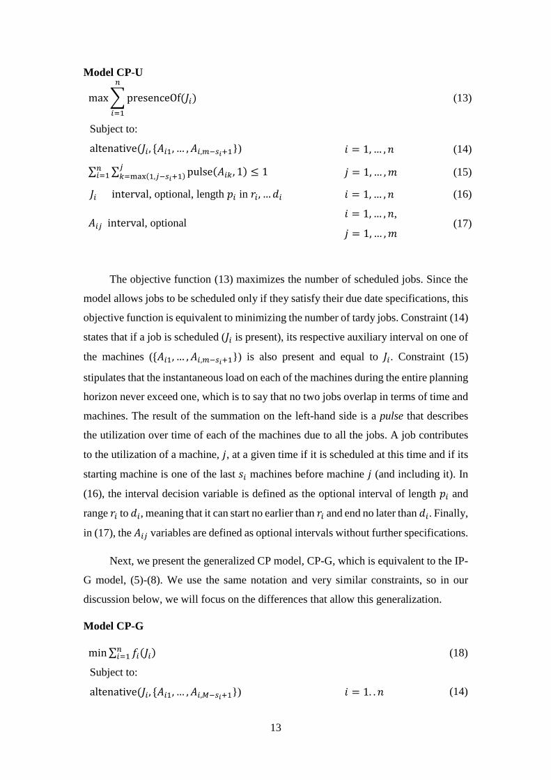
The objective function (13) maximizes the number of scheduled jobs. Since the

model allows jobs to be scheduled only if they satisfy their due date specifications, this

objective function is equivalent to minimizing the number of tardy jobs. Constraint (14)

states that if a job is scheduled (𝐽𝑖 is present), its respective auxiliary interval on one of

the machines ({𝐴𝑖1, … , 𝐴𝑖,𝑚−𝑠𝑖+1}) is also present and equal to 𝐽𝑖. Constraint (15)

stipulates that the instantaneous load on each of the machines during the entire planning

horizon never exceed one, which is to say that no two jobs overlap in terms of time and

machines. The result of the summation on the left-hand side is a pulse that describes

the utilization over time of each of the machines due to all the jobs. A job contributes

to the utilization of a machine, 𝑗, at a given time if it is scheduled at this time and if its

starting machine is one of the last 𝑠𝑖 machines before machine 𝑗 (and including it). In

(16), the interval decision variable is defined as the optional interval of length 𝑝𝑖 and

range 𝑟𝑖 to 𝑑𝑖, meaning that it can start no earlier than 𝑟𝑖 and end no later than 𝑑𝑖. Finally,

in (17), the 𝐴𝑖𝑗 variables are defined as optional intervals without further specifications.

Next, we present the generalized CP model, CP-G, which is equivalent to the IP-

G model, (5)-(8). We use the same notation and very similar constraints, so in our

discussion below, we will focus on the differences that allow this generalization.

Model CP-G

min∑ 𝑓𝑖(𝐽𝑖)𝑛𝑖=1 (18)

Subject to:

altenative(𝐽𝑖, {𝐴𝑖1, … , 𝐴𝑖,𝑀−𝑠𝑖+1}) 𝑖 = 1. . 𝑛 (14)

14

∑ ∑ pulse(𝐴𝑖𝑘, 1)𝑗𝑘=max(1,𝑗−𝑠𝑖+1)

𝑛𝑖=1 ≤ 1 𝑗 = 1. . 𝑚, (15)

𝐽𝑖, Interval, length 𝑝𝑖 in 𝑟𝑖, … 𝑇 𝑖 = 1. . 𝑛 (19)

𝐴𝑖𝑗, Interval, optional 𝑖 = 1. . 𝑛, 𝑗 = 1. . 𝑚 (17)

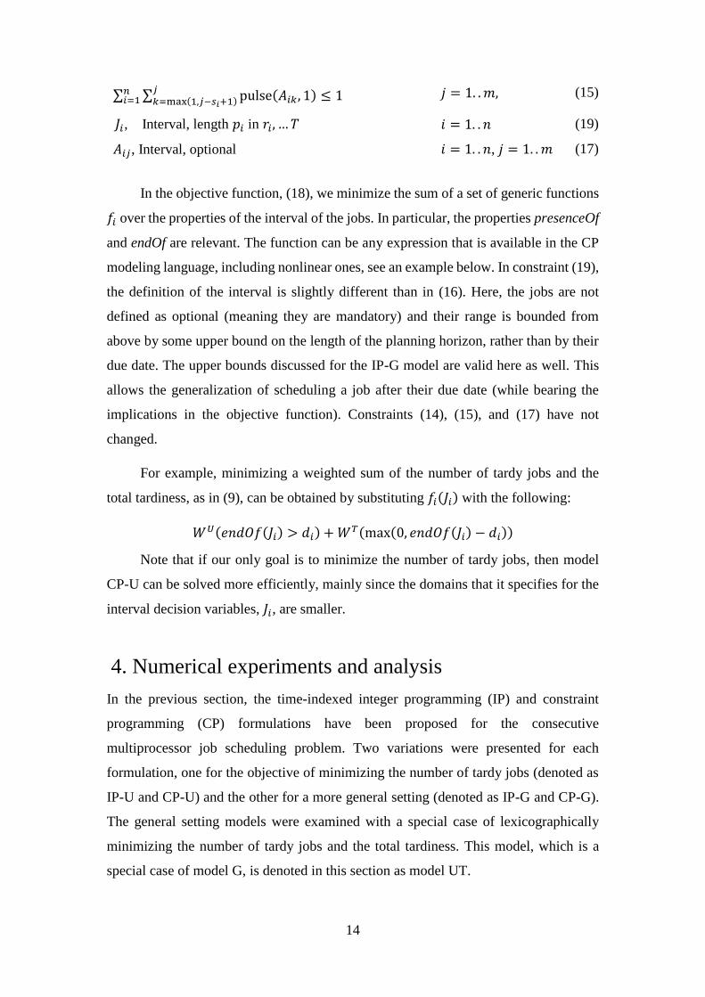
In the objective function, (18), we minimize the sum of a set of generic functions

𝑓𝑖 over the properties of the interval of the jobs. In particular, the properties presenceOf

and endOf are relevant. The function can be any expression that is available in the CP

modeling language, including nonlinear ones, see an example below. In constraint (19),

the definition of the interval is slightly different than in (16). Here, the jobs are not

defined as optional (meaning they are mandatory) and their range is bounded from

above by some upper bound on the length of the planning horizon, rather than by their

due date. The upper bounds discussed for the IP-G model are valid here as well. This

allows the generalization of scheduling a job after their due date (while bearing the

implications in the objective function). Constraints (14), (15), and (17) have not

changed.

For example, minimizing a weighted sum of the number of tardy jobs and the

total tardiness, as in (9), can be obtained by substituting 𝑓𝑖(𝐽𝑖) with the following:

𝑊𝑈(𝑒𝑛𝑑𝑂𝑓(𝐽𝑖) > 𝑑𝑖) +𝑊𝑇(max(0, 𝑒𝑛𝑑𝑂𝑓(𝐽𝑖) − 𝑑𝑖))

Note that if our only goal is to minimize the number of tardy jobs, then model

CP-U can be solved more efficiently, mainly since the domains that it specifies for the

interval decision variables, 𝐽𝑖, are smaller.

4. Numerical experiments and analysis

In the previous section, the time-indexed integer programming (IP) and constraint

programming (CP) formulations have been proposed for the consecutive

multiprocessor job scheduling problem. Two variations were presented for each

formulation, one for the objective of minimizing the number of tardy jobs (denoted as

IP-U and CP-U) and the other for a more general setting (denoted as IP-G and CP-G).

The general setting models were examined with a special case of lexicographically

minimizing the number of tardy jobs and the total tardiness. This model, which is a

special case of model G, is denoted in this section as model UT.

15

In addition to the IP and CP formulation, we examine, as a benchmark, a

modified version of the mixed integer programming formulation originally presented

in (Guan & Cheung, 2004), denoted as GC. Since, to the best of our knowledge, the

model proposed here has not been studied in the literature, we adapt the (Guan &

Cheung, 2004) formulation, which is based on continuous variables for the position of

the jobs and integer variables for non-overlapping constraints. Then, we modify the

objective of the original formulation, first for minimizing the number of tardy jobs

(denoted CG-U) and then for the lexicographic problem (denote as CG-UT). Note that

this formulation is also similar to other formulations suggested for the facility layout

problems, see (Heragu, 2008). Our adaptation is presented in Appendix A.

Next, we compare the performance of the three formulations, for each of the

problem types, presented above. Other than the general relative performance of the

formulations, we study the effect of the problem parameters on the performance and

identify the classes in which each formulation performs best.

4.1. Experimental design

A full factorial design experimentation was conducted. The instances for each of the

two problems (denoted as U and G) were solved using the three formulations (GC, IP,

and CP). The factors in our design are as follows:

1. The number of machines, 𝑚, with two levels of 15 and 25;

2. The number of jobs, 𝑛, with five levels of 10, 20, 30, 40, and 50;

3. The time granulation of the job’s processing time. For each job 𝑖, a process time,𝑝𝑖,

is drawn from a discrete uniform distribution 𝑈(𝑝𝑚𝑎𝑥

5, 𝑝𝑚𝑎𝑥), where 𝑝𝑚𝑎𝑥 is a

parameter responsible for the time granulation. Five levels were given to this

parameter: 5, 10, 20, 40 and 80. For example, 𝑝𝑚𝑎𝑥 = 5 indicates that the

processing time is taken from a discrete distribution with possible discrete values

of 1 to 5. When 𝑝𝑚𝑎𝑥 = 40, for example, a higher granulation processing time is

considered, which is taken from a discrete distribution with possible discrete values

of 8 to 40.

4. The job size, namely, the number of consecutive machines it requires. The size of

job 𝑖, 𝑠𝑖, is drawn from discrete uniform distribution 𝑈(1, ⌊𝑠 ⋅ 𝑚⌋), where ⌊𝑥⌋ is the

largest integer that is smaller than or equal to 𝑥, and the factor 𝑠 has two levels of

0.3 and 0.5.

16

5. Two tightness levels of the window between the ready time and the due dates as

described below.

The factors and their levels are depicted in Table 1. In summary, the full factorial

experiment results in 2 × 5 × 5 × 2 × 2 = 200 instances for each of the six models,

1200 runs in total. The solvers’ running time was limited to 10 minutes but in most of

the instances the solution process was terminated with a provably optimal solution

earlier.

The ready times and due dates of the jobs were set to maintain two structures of the

problems, with different levels of tightness. The values of the tightness parameters were

determined via preliminary experiments, to avoid extreme cases of none or too many

tardy jobs; cases that were found to be very easy to solve. Consequently, the structure

with the high tightness resulted in an average of around 25% tardy jobs, while the

structure with the low tightness resulted in an average of around 5% tardy jobs. The

procedure of setting the corresponding parameters was done as follows. The ready time

of each job 𝑖, 𝑟𝑖, was randomly drawn from the set {0,1, … , Δ𝑚𝑎𝑥} and the due date was

taken from the set {𝑟𝑖 + 𝑝𝑖, 𝑟𝑖 + 𝑝𝑖 + 1,… , 𝑟𝑖 + 𝑝𝑖 + Δ𝑚𝑎𝑥}, while keeping the value of

Δ𝑚𝑎𝑥 proportional to the capacity required by the scheduled jobs. Specifically, we set

Δ𝑚𝑎𝑥 = 𝜁�̅� ∙ �̅� ∙ 𝑛/𝑚, where �̅� is the average processing time and �̅� is the average job

size. The parameter 𝜁 represents the level of tightness, with values of 0.3 for the tight

instances, and 0.6 for the loose ones.

The length of the planning horizon in the UT problem was set based on the upper

bound obtained from (11) and (12), using the best solution obtained for the equivalent

U model.

Table 1: Factors summary

Factor Set of possible values

𝑚 Number of machines {15, 25} 𝑛 Number of jobs {10, 20, 30, 40, 50}

𝑝𝑚𝑎𝑥 Max. process time (resolution) {5, 10, 20, 40, 80} 𝑠 Job size factor {0.3, 0.5} 𝜁 Tightness level of the instance {0.3, 0.6}

The experiments were conducted on an Intel i7-6700K desktop with 64 GB Ram

running under Windows 10. We use Cplex Studio 12.8 to formulate and solve all the

17

six models. The input files, the Python code that was used to generate it, and the OPL

models are available upon request from the second author.

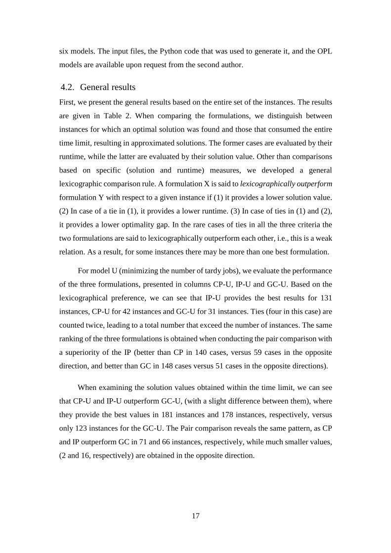
4.2. General results

First, we present the general results based on the entire set of the instances. The results

are given in Table 2. When comparing the formulations, we distinguish between

instances for which an optimal solution was found and those that consumed the entire

time limit, resulting in approximated solutions. The former cases are evaluated by their

runtime, while the latter are evaluated by their solution value. Other than comparisons

based on specific (solution and runtime) measures, we developed a general

lexicographic comparison rule. A formulation X is said to lexicographically outperform

formulation Y with respect to a given instance if (1) it provides a lower solution value.

(2) In case of a tie in (1), it provides a lower runtime. (3) In case of ties in (1) and (2),

it provides a lower optimality gap. In the rare cases of ties in all the three criteria the

two formulations are said to lexicographically outperform each other, i.e., this is a weak

relation. As a result, for some instances there may be more than one best formulation.

For model U (minimizing the number of tardy jobs), we evaluate the performance

of the three formulations, presented in columns CP-U, IP-U and GC-U. Based on the

lexicographical preference, we can see that IP-U provides the best results for 131

instances, CP-U for 42 instances and GC-U for 31 instances. Ties (four in this case) are

counted twice, leading to a total number that exceed the number of instances. The same

ranking of the three formulations is obtained when conducting the pair comparison with

a superiority of the IP (better than CP in 140 cases, versus 59 cases in the opposite

direction, and better than GC in 148 cases versus 51 cases in the opposite directions).

When examining the solution values obtained within the time limit, we can see

that CP-U and IP-U outperform GC-U, (with a slight difference between them), where

they provide the best values in 181 instances and 178 instances, respectively, versus

only 123 instances for the GC-U. The Pair comparison reveals the same pattern, as CP

and IP outperform GC in 71 and 66 instances, respectively, while much smaller values,

(2 and 16, respectively) are obtained in the opposite direction.

18

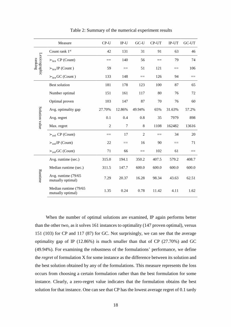
Table 2: Summary of the numerical experiment results

Measure CP-U IP-U GC-U CP-UT IP-UT GC-UT

Lex

icog

raph

ic

rank

ing

Count rank 1st 42 131 31 91 63 46

≻𝑙𝑒𝑥 CP (Count) == 140 56 == 79 74

≻𝑙𝑒𝑥IP (Count ) 59 == 51 121 == 106

≻𝑙𝑒𝑥GC (Count ) 133 148 == 126 94 ==

So

lutio

n v

alue

Best solution 181 178 123 100 87 65

Number optimal 151 161 117 80 76 72

Optimal proven 103 147 87 70 76 60

Avg. optimality gap 27.70% 12.86% 49.94% 65% 31.63% 57.2%

Avg. regret 0.1 0.4 0.8 35 7979 898

Max. regret 2 7 8 1108 162482 13616

≻𝑠𝑜𝑙 CP (Count) == 17 2 == 34 20

≻𝑠𝑜𝑙IP (Count) 22 == 16 90 == 71

≻𝑠𝑜𝑙GC (Count) 71 66 == 102 61 ==

Ru

ntim

e

Avg. runtime (sec.) 315.0 194.1 350.2 407.5 579.2 408.7

Median runtime (sec.) 311.5 147.7 600.0 600.0 600.0 600.0

Avg. runtime (79/65

mutually optimal) 7.29 20.37 16.28 98.34 43.63 62.51

Median runtime (79/65

mutually optimal) 1.35 0.24 0.78 11.42 4.11 1.62

When the number of optimal solutions are examined, IP again performs better

than the other two, as it solves 161 instances to optimality (147 proven optimal), versus

151 (103) for CP and 117 (87) for GC. Not surprisingly, we can see that the average

optimality gap of IP (12.86%) is much smaller than that of CP (27.70%) and GC

(49.94%). For examining the robustness of the formulations’ performance, we define

the regret of formulation X for some instance as the difference between its solution and

the best solution obtained by any of the formulations. This measure represents the loss

occurs from choosing a certain formulation rather than the best formulation for some

instance. Clearly, a zero-regret value indicates that the formulation obtains the best

solution for that instance. One can see that CP has the lowest average regret of 0.1 tardy

19

jobs, with a maximal value of 2. Namely, for all cases where CP trailed other

formulations, the difference was at most two tardy jobs. IP and GC, on the other hand,

have an average regret value of 0.4 and 0.8 tardy jobs, with a maximal value of 7 and

8, respectively.

To complete the analysis, we examine the runtime performance, where we

distinguish between the runtime of all instances and the runtime of instances that were

solved to optimality by all formulations (mutually optimal). For the U problem, 79

mutually optimal instances were identified. When all instances are considered, one can

see that IP-U outperforms the other two formulations providing a much smaller average

runtime of 194.1 seconds, versus 315.0 for CP-U and 350.2 for GC-U. Same ranking is

obtained for the median, however, where the median is smaller than the average for IP

and CP, it is not the case for the GC, which provides a median of 600 second. This

indicates that more than half of the problems solved by the GC used all the allotted

runtime.

When the lexicographic objective is considered (minimizing the number of tardy

jobs and the total tardiness, as a primary and a secondary objective, respectively – see

columns CP-UT, IP-UT, and GC-UT in the table), the CP performs much better, and

outperforms IP and GC in most performance measures. Considering the lexicographic

preference, the CP is counted first in 91 instances, versus 63 for the IP and 46 for the

GC. In the pair comparison, the CP is much better than the other two formulations,

while the GC is slightly better than the IP.

When the solution value is examined, the same ranking is obtained, both for the

number of best solution obtained in each formulation (100 for the CP, 87 for the IP and

65 for the GC), and for the number of optimal solutions obtained for each formulation

(80 for the CP, 76 for the IP and 72 for the GC). When only proven optimal solutions

are considered, the IP performs better than the other two formulations, as all 76 optimal

solutions are proven, versus 70 out of 80 for the CP and 60 out of 72 for the GC. This

is probably since the IP provides better bounds than the other formulations, with an

average optimality gap of 31.16% versus 57.2% for the GC and 65% for the CP. The

last performance measure associated with the solution value is the average and max

regret, explained above. As for the U formulations, the CP is significantly outperforms

the other formulations also in UT, both for the average and maximal regret. This

20

measure is highly important, because it indicates that even when the CP does not

provide the best solution, the amount of loss versus the best formulation for that

instance is relatively low.

When considering the runtime, we distinguish again between the whole set of

instances and the set of mutually optimal instances. One can see that in the first case,

the CP and GC outperforms IP with respect to the average runtime, however, all the

formulation provide a median value of 600 second. This is because the UT problem is

harder to solve than the U problem, and in many of the instances require the maximal

runtime in all formulations. Interestingly, when the mutually optimal instances are

considered (65 out of 200), the IP provides the lowest average runtime, while the GC

has the lowest average median. This is probably because the CP requires in general

large runtime when providing an optimal solution, due to the large optimality gap,

versus the other formulations.

To conclude the general results, we can see that the IP performs best when the U

problems are considered. Still, when considering the robust performance, the CP is

recommended, with a much smaller average and maximal regret. When considering the

UT problems, the CP provides the best performance, both when the solution value,

runtime and robustness measures are considered.

4.3. The effect of the problem parameters on the performance

In this section, we examine the effect of the problem parameters on the relative

performance of the three formulations to design a recommended scheme for choosing

the best formulation(s) to use for each combination of parameters. This problem is

actually a classification problem, where the aim is to provide a prediction model to

suggest the best formulation to use for each given instance. To this end, we have chosen

to adopt a decision tree approach solve by CHAID (Chi-square automatic interaction

detection) algorithm (Kass, 1980). The algorithm was executed on SPSS software.

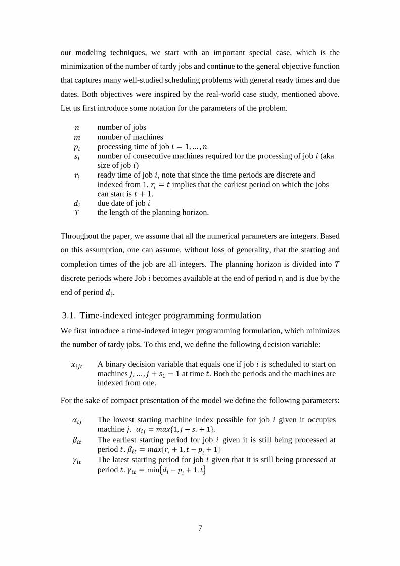
First, a decision tree was constructed to compare each formulation with the others.

Hence, when examining a particular formulation, the purpose is to predict whether this

formulation will provide the best solution (among the three formulations) for a given

parameter combination, or not. The runtime limit was set to 10 minutes in this

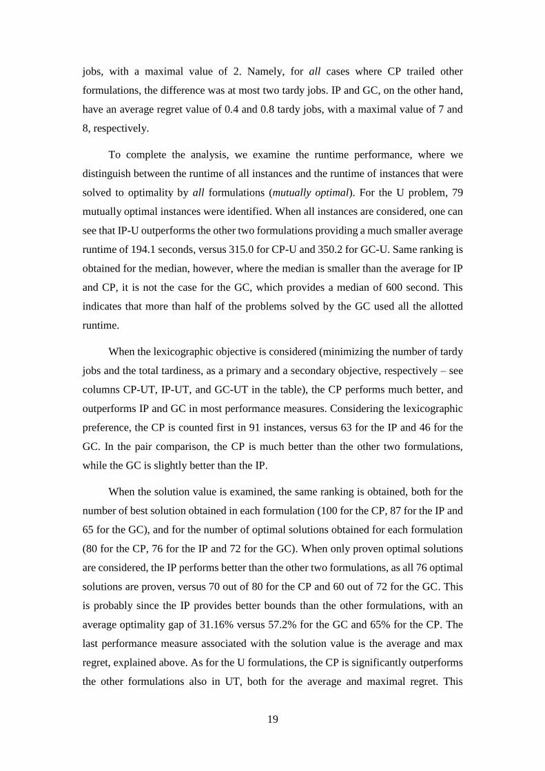
experiment. The results are shown in Figure 3, where the tree on the left refers to the

IP model and the tree on the right to the GC model. Each inner node in the tree indicates

21

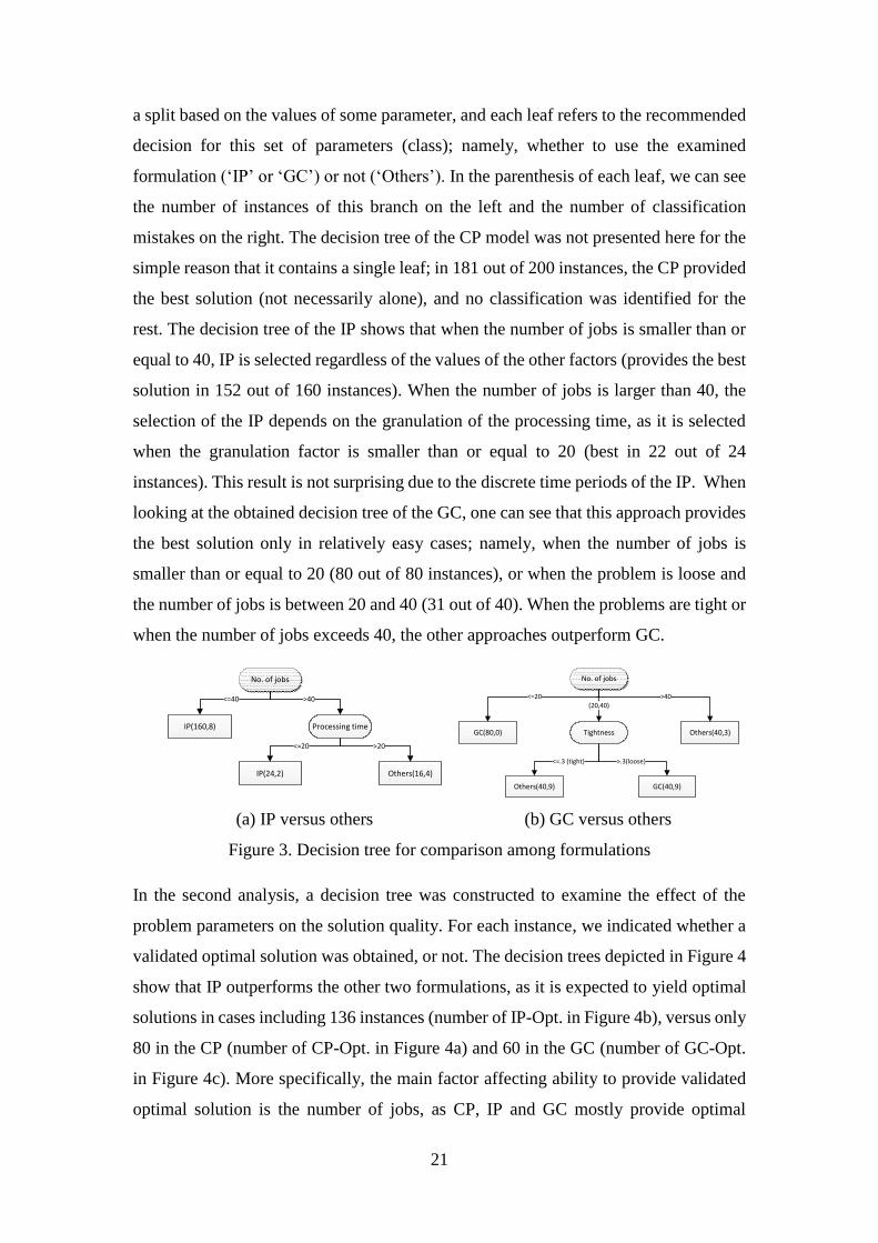
a split based on the values of some parameter, and each leaf refers to the recommended

decision for this set of parameters (class); namely, whether to use the examined

formulation (‘IP’ or ‘GC’) or not (‘Others’). In the parenthesis of each leaf, we can see

the number of instances of this branch on the left and the number of classification

mistakes on the right. The decision tree of the CP model was not presented here for the

simple reason that it contains a single leaf; in 181 out of 200 instances, the CP provided

the best solution (not necessarily alone), and no classification was identified for the

rest. The decision tree of the IP shows that when the number of jobs is smaller than or

equal to 40, IP is selected regardless of the values of the other factors (provides the best

solution in 152 out of 160 instances). When the number of jobs is larger than 40, the

selection of the IP depends on the granulation of the processing time, as it is selected

when the granulation factor is smaller than or equal to 20 (best in 22 out of 24

instances). This result is not surprising due to the discrete time periods of the IP. When

looking at the obtained decision tree of the GC, one can see that this approach provides

the best solution only in relatively easy cases; namely, when the number of jobs is

smaller than or equal to 20 (80 out of 80 instances), or when the problem is loose and

the number of jobs is between 20 and 40 (31 out of 40). When the problems are tight or

when the number of jobs exceeds 40, the other approaches outperform GC.

(a) IP versus others (b) GC versus others

Figure 3. Decision tree for comparison among formulations

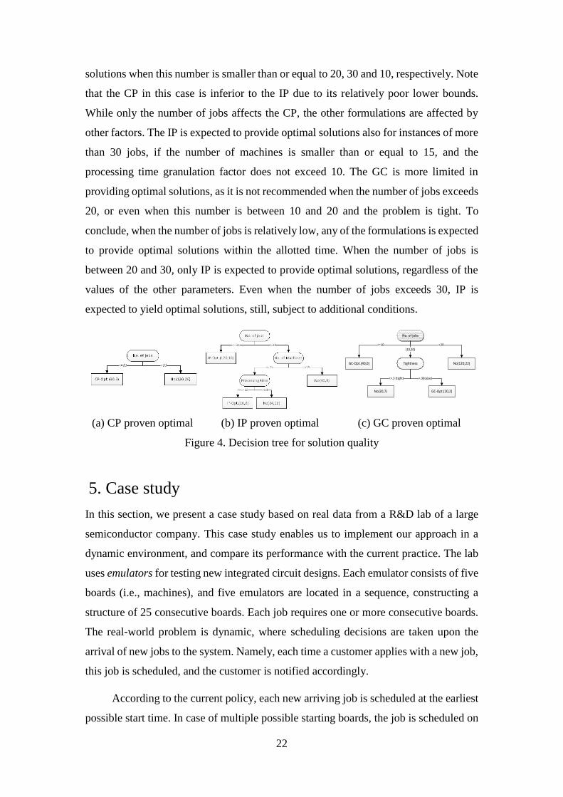
In the second analysis, a decision tree was constructed to examine the effect of the

problem parameters on the solution quality. For each instance, we indicated whether a

validated optimal solution was obtained, or not. The decision trees depicted in Figure 4

show that IP outperforms the other two formulations, as it is expected to yield optimal

solutions in cases including 136 instances (number of IP-Opt. in Figure 4b), versus only

80 in the CP (number of CP-Opt. in Figure 4a) and 60 in the GC (number of GC-Opt.

in Figure 4c). More specifically, the main factor affecting ability to provide validated

optimal solution is the number of jobs, as CP, IP and GC mostly provide optimal

No. of jobs

IP(160,8)

IP(24,2)

<=40 >40

<=20 >20

Others(16,4)

Processing time

No. of jobs

GC(80,0)

Others(40,9)

<=20(20,40)

GC(40,9)

Tightness Others(40,3)

>40

<=.3 (tight) >.3(loose)

22

solutions when this number is smaller than or equal to 20, 30 and 10, respectively. Note

that the CP in this case is inferior to the IP due to its relatively poor lower bounds.

While only the number of jobs affects the CP, the other formulations are affected by

other factors. The IP is expected to provide optimal solutions also for instances of more

than 30 jobs, if the number of machines is smaller than or equal to 15, and the

processing time granulation factor does not exceed 10. The GC is more limited in

providing optimal solutions, as it is not recommended when the number of jobs exceeds

20, or even when this number is between 10 and 20 and the problem is tight. To

conclude, when the number of jobs is relatively low, any of the formulations is expected

to provide optimal solutions within the allotted time. When the number of jobs is

between 20 and 30, only IP is expected to provide optimal solutions, regardless of the

values of the other parameters. Even when the number of jobs exceeds 30, IP is

expected to yield optimal solutions, still, subject to additional conditions.

(a) CP proven optimal (b) IP proven optimal (c) GC proven optimal

Figure 4. Decision tree for solution quality

5. Case study

In this section, we present a case study based on real data from a R&D lab of a large

semiconductor company. This case study enables us to implement our approach in a

dynamic environment, and compare its performance with the current practice. The lab

uses emulators for testing new integrated circuit designs. Each emulator consists of five

boards (i.e., machines), and five emulators are located in a sequence, constructing a

structure of 25 consecutive boards. Each job requires one or more consecutive boards.

The real-world problem is dynamic, where scheduling decisions are taken upon the

arrival of new jobs to the system. Namely, each time a customer applies with a new job,

this job is scheduled, and the customer is notified accordingly.

According to the current policy, each new arriving job is scheduled at the earliest

possible start time. In case of multiple possible starting boards, the job is scheduled on

No. of jobs

GC-Opt.(40,0)

No(20,7)

<=10(10,20)

GC-Opt.(20,2)

Tightness No(120,22)

>20

<=.3 (tight) >.3(loose)

23

the smallest indexed board. Once a schedule of a job is determined, this scheduled is

final, and no rescheduling of this job is considered later on.

We propose integrating our IP and CP formulations in this dynamic environment,

using a rolling horizon scheme. Namely, each time a customer applies to the system

with a new job(s), the scheduling problem is solved by using one of our mathematical

formulations, subject to the current state of the system, and commitments already made

to previous customers. The formulation is solved each time with a lexicographic multi-

objective function, with the number of tardy jobs as the primary objective and the total

tardiness as the secondary one. In cases of ties, jobs are scheduled at the earliest possible

time.

Once the model is solved, a commitment to the customer is made regarding the

completion time. Two types of commitments are considered: (1) exact completion time

of the newly scheduled job(s), as obtained by the model solution; and (2) satisfying the

requested due date, if possible, or the completion time obtained from the model,

otherwise. The former type is denoted by exact commitment (EC), and the latter by due-

date commitment (DC). Note that the due-date commitment is looser than the exact

commitment since some slack may occur in this case between the obtained completion

time and the requested due-date. This slack may be used later on in rescheduling the

existing jobs upon the arrival of new jobs. Rescheduling is also possible in the exact

commitment; however, it is limited to the identity of the machines assigned to the job.

Our CP and IP models were modified to capture the nature of the dynamic

environment. To this end, three types of jobs are defined upon the arrival of new jobs

at the system, as follows: (1) jobs in progress (running jobs); (2) already scheduled jobs

– not yet running; and (3) newly arriving job(s). The models are solved, starting from

the current time with additional constraints that stipulate the schedule of the type 1 jobs

and impose hard due-dates upon type 2 jobs, based on the commitment type (EC or

DC). The type 3 jobs are freely scheduled. The two modified models are presented in

Appendix C.

Our case study was based on historical data obtained from the R&D lab. We

created a simulation environment that allows for the examination of the current

scheduling policy and the rolling horizon policy using our formulations. The numerical

study was performed using three log files of customers’ requests. The log files contain

24

information on the arrival time, the requested processing time and the number of boards

required by each job. The ready times were taken as the arrival times of the jobs. The

due date property of the jobs was missing, so it was randomly generated in between the

minimal possible completion time (𝑟𝑖 + 𝑝𝑖) and the end the current week. According to

the lab manager, these assumptions are in line with the current practice in the lab. The

processing times and due dates in the log file are specified in units of half hours and

there are cases where several jobs became available simultaneously. Each log file

contains 171-288 jobs to be processed within a horizon of 37-60 days (1776-2880 time

units). The characteristics of the datasets are given in Table 3.

Two runtime limits of 30 and 600 seconds were decided for each run. Each value

may correspond to a different real-world situation, which is based on the urgency of the

feedback to the customer. Note that applying the formulation in a rolling horizon

scheme results in a myopic heuristic procedure, so their performance is not necessarily

better than the existing greedy policy. Moreover, while increasing the runtime improves

the accuracy of the obtained solution at each run, it does not necessarily improve the

schedule.

Table 3. Characteristics of the datasets.

No. of

jobs

Planning

horizon

Avg. (STD)

process time

(hours)

Min (Max)

process time

(hours)

Avg. (STD)

job size

(boards)

Min (Max)

job size

(boards)

Dataset 1 288 60 days 4.5 (9.9) 0.5 (168) 12 (4.6) 1 (25)

Dataset 2 196 37 days 6.7 (5.2) 0.5 (24) 12 (5.5) 1 (25)

Dataset 3 171 53 days 14.8 (5.2) 0.5 (72) 13 (5.3) 1 (25)

Table 4 presents the number of tardy jobs and the total tardiness of the three

datasets for the current policy as well as for the two formulation based algorithm (CP

and IP) under the two commitment types (EC, DC). In general, one can see that even

for the lower time limit of 30 seconds, the procedure using the CP formulation

outperformed the current policy in all cases. Although a significant improvement was

obtained for the cases of the EC commitment type, a much larger improvement was

achieved when the DC commitment type was considered, due to the further flexibility

in the rescheduling process. For example, the number of tardy jobs was reduced from

22 to 8 in dataset 1, from 24 to 1 in dataset 2, and from 27 to 11 in dataset 3. When the

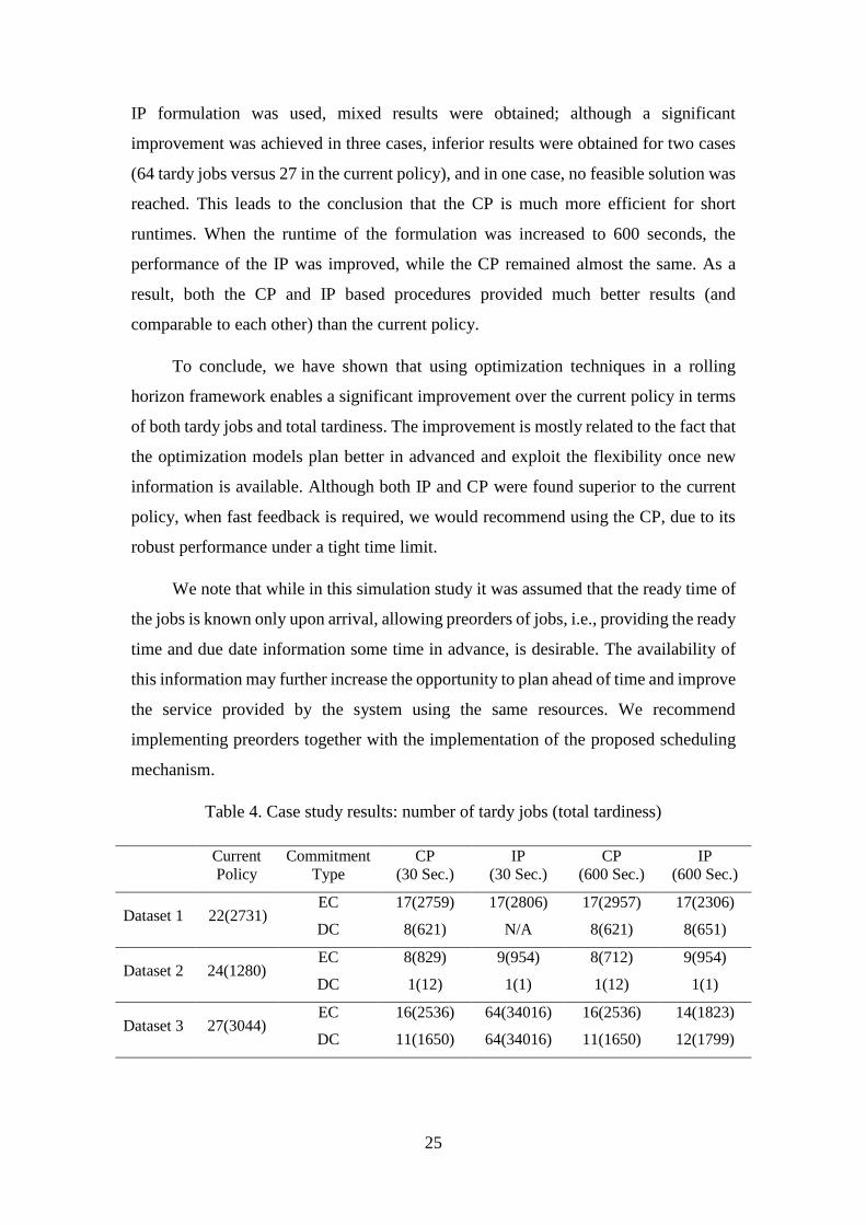
25

IP formulation was used, mixed results were obtained; although a significant

improvement was achieved in three cases, inferior results were obtained for two cases

(64 tardy jobs versus 27 in the current policy), and in one case, no feasible solution was

reached. This leads to the conclusion that the CP is much more efficient for short

runtimes. When the runtime of the formulation was increased to 600 seconds, the

performance of the IP was improved, while the CP remained almost the same. As a

result, both the CP and IP based procedures provided much better results (and

comparable to each other) than the current policy.

To conclude, we have shown that using optimization techniques in a rolling

horizon framework enables a significant improvement over the current policy in terms

of both tardy jobs and total tardiness. The improvement is mostly related to the fact that

the optimization models plan better in advanced and exploit the flexibility once new

information is available. Although both IP and CP were found superior to the current

policy, when fast feedback is required, we would recommend using the CP, due to its

robust performance under a tight time limit.

We note that while in this simulation study it was assumed that the ready time of

the jobs is known only upon arrival, allowing preorders of jobs, i.e., providing the ready

time and due date information some time in advance, is desirable. The availability of

this information may further increase the opportunity to plan ahead of time and improve

the service provided by the system using the same resources. We recommend

implementing preorders together with the implementation of the proposed scheduling

mechanism.

Table 4. Case study results: number of tardy jobs (total tardiness)

Current

Policy

Commitment

Type

CP

(30 Sec.)

IP

(30 Sec.)

CP

(600 Sec.)

IP

(600 Sec.)

Dataset 1 22(2731) EC 17(2759) 17(2806) 17(2957) 17(2306)

DC 8(621) N/A 8(621) 8(651)

Dataset 2 24(1280) EC 8(829) 9(954) 8(712) 9(954)

DC 1(12) 1(1) 1(12) 1(1)

Dataset 3 27(3044) EC 16(2536) 64(34016) 16(2536) 14(1823)

DC 11(1650) 64(34016) 11(1650) 12(1799)

26

6. Conclusion

In this study, we introduced two effective optimization models for the consecutive

multiprocessor job scheduling problem. We studied the objective function of

minimizing the number of tardy jobs as well as minimizing a weighted sum of the

number of tardy jobs and total tardiness. However, our model is amenable to a rich set

of objective functions, including nonlinear and non-convex ones.

The effectiveness of our model was demonstrated by an extensive numerical

study, and its applicability to real-life problems was demonstrated by embedding a

rolling horizon version of the algorithm in a simulation of an actual on-line production

environment. We showed that both the number of tardy jobs and the total tardiness

could be reduced significantly.

While both our time-indexed IP and CP models were shown to be more effective

on average than our adaptation of the GC formulations known from the literature, none

of the three tested methods completely dominates the others. The IP model is good for

obtaining optimal solutions quickly when the time granularity is rough, which we

believe is the case in many actual manufacturing environments. It also provides a strong

lower bound for the solutions, which is a nice theoretical trait that is not necessarily

important for practitioners. The CP models delivered the best solutions in most of our

experiments and was found the most robust approach, while lags behind the other

methods by a tiny gap in the few cases when it did not find the best solution. The GC

models are insensitive to the time granularity and thus can be useful when the accuracy

of the time input is high. However, the lower bounds established by the GC model are

very weak.

There are several interesting directions for future research based on the results of

this study. In particular, the effectiveness of time-indexed integer formulations and

constraint programming formulations as practical solution methods for other variants

of the multiprocessor job scheduling problem should be verified. Since time-indexed

formulations are especially effective when the time granulation is low, this naturally

leads to two step heuristic methods in which the sequence of the jobs is decided based

on a model with a rough time granulation, after rounding the original input, and the

schedule is then fine-tuned to respect the accurate times. The effect of rough time

27

granulation is of particular interest in an online situation when tentative decisions about

the future need to be made quickly.

References

Agra, A., & Oliveira, M. (2018). MIP approaches for the integrated berth allocation

and quay crane assignment and scheduling problem. European Journal of

Operational Research, 264, 138-148.

Apt, K. Y. (2003). Principles of Constraint Programming (1 ed.). Amsterdam:

Cambridge University Press.

Baptiste, P. (2003). A note on scheduling multiprocessor tasks with identical

processing times. Computers & Operations Research, 30, 2071-2078.

Bianco, L., Blazewicz, J., Dell'Olmo, P., & Drozdowski, M. (1995). Scheduling

multiprocessor tasks on a dynamic configuration of dedicated processors.

Annals of Operations Research, 58, 493-517.

Bierwirth, C., & Meisel, F. (2010). A survey of berth allocation and quay crane

scheduling problems in container terminals. European Journal of Operational

Research, 202, 615-627.

Bukchin, Y., & Raviv, T. (2018). Constraint programming for solving various

assembly line balancing problems. Omega, 78, 57-68.

Chen, J., & Lee, C. Y. (1999). General multiprocessor task scheduling. Naval

Research Logistics, 46, 57-74.

Ernst, A. T., Oguz, C., Singh, G., & Taherkhani, G. (2017). Mathematical models for

the berth allocation problem in dry bulk terminals. Journal of Scheduling, 20,

459-473.

Guan, Y., & Cheung, K. R. (2004). The berth allocation problem models and solution

methods. OR Spectrum, 75-92.

Heragu, S. (2008). Facilities Design. CRC Press.

Huang, J., Chen, J. C., & Wang, J. (2007). A simple linear time approximation

algorithm for multiprocessor job scheduling on four processors. Journal of

Combinatorial Optimization, 13, 33-45.

IBM. (2009). Detailed Scheduling in IBM ILOG OPL with IBM ILOG CP Optimizer -

Tutorial. IBM Corp.

Imai, A., Chia, C. H., Etsuko, N., & Papadimitriou, S. (2008). The simultaneous berth

and quay crane allocation problem. Transportation Research Part E, 900-920.

28

Imai, A., Nishimura, E., & Papadimitriou, S. (2001). The dynamic berth allocation

problem for a container port. Transportation Research Part B:

Methodological, 35, 401-417.

Imai, A., Sun, X., Nishimura, E., & Papadimitriou, S. (2005). Berth allocation in a

container port using a continuous location space approach. Transportation

Research Part B, 39, 199-221.

Kass, G. (1980). An exploratory technique for investigating large quantities of

categorical data. Journal of the Royal Statistical Society: Series C (Applied

Statistics), 29(2), 119-127.

Leonardi, S., & Raz, D. (2007). Approximating total flow time on parallel machines.

Journal of Computer and System Sciences, 73, 875–891.

Martello, S., Monaci, M., & Vigo, D. (2003). An exact approach to the strip-packing

problem. INFORMS Journal on Computing, 15(3), 310-319.

Moon, K. (2000). A Mathematical Model and a Heuristic Algorithm for Berth

Planning. Ph.D. Thesis, Pusan National University, Pusan.

Park, Y. M., & Kim, K. H. (2005). A scheduling method for berth and quay cranes.

Container Terminals and Automated Transport Systems, 159-181.

Pinedo, M. L. (2012). Scheduling: Theory, Algorithms, and Systems, Fourth Edition.

New York: Springer.

Sevaux, M., & Thomin, P. (2001). Heuristics and metaheuristics for a parallel

machine schedulign problem: a computational evaluation. Proceedings of the

4th Metaheuristics International Conference, (pp. 411-415).

Shaw, P. (1998). Using constraint programming and local search methods to solve

vehicle routing problems. International Conference on Principles and

Practice of Constraint Programming. (pp. 417-431). Berlin Heidelberg:

Springer.

Umang, N., Bierlaire, M., & Vacca, I. (2013). Exact and heuristic method to solve

berth allocation problem in bulk ports. Transportation Research Part E, 54,

14-31.

Appendix A - Relative position MILP formulation

In this appendix, we present a relative position MILP formulation to our problem

adopted from (Guan & Cheung, 2004) with minor modifications to reflect our objective

function. The original formulation minimizes the weighted flow time. Similar relative

position formulations were presented in (Moon, 2000) and (Imai, Sun, Nishimura, &

Papadimitriou, 2005) for the berth allocation problem and in (Heragu, 2008) for the

29

facilities layout problem. It is presented here since we used it to benchmark our integer

programming and CP formulation.

We use the same notation for the model parameters as presented in Section 3 and

introduce the following decision variables:

𝑥𝑖 start time of job 𝑖

𝑦𝑖 first machine occupied by job 𝑖

𝜎𝑖𝑗 = {1, if job 𝑖 ends before job 𝑗 starts0, otherwise

𝛿𝑖𝑗 = {1, if job 𝑖 ends on amachine withsmaller indexthan thefirst machineof job 𝑗0, otherwise

𝑈𝑖 = {1, if job 𝑖 istardy0, otherwise

𝑇𝑖 The tardiness of job 𝑖

The model presented below implements a special case of our general IP and CP

models, where the objective is to minimize a weighted sum of the number of tardy jobs

and the total tardiness. The model presented below captures the case of minimizing the

number of tardy jobs. Note, however, that other interesting objective functions, such as

a nonlinear penalty for tardiness, are not directly represented by this model.

min {𝑊𝑈∑𝑈𝑖

𝑛

𝑖=1

+𝑊𝑇∑𝑇𝑖

𝑛

𝑖=1

}

(20)

Subject to:

𝑈𝑖 × 𝑇 ≥ 𝑐𝑖 − 𝑑𝑖 ∀𝑖 = 1, … , 𝑛 (21)

𝑥𝑗 ≥ 𝑐𝑖 − (1 − 𝜎𝑖𝑗)𝑇 ∀𝑖, 𝑗 = 1,… , 𝑛 (22)

𝑦𝑗 ≥ 𝑦𝑖 + 𝑠𝑖 − (1 − 𝛿𝑖𝑗)𝑚 ∀𝑖, 𝑗 = 1,… , 𝑛 (23)

𝜎𝑖𝑗 + 𝜎𝑗𝑖 + 𝛿𝑖𝑗 + 𝛿𝑗𝑖 ≥ 1 ∀𝑖, 𝑗 = 1,… , 𝑛 (24)

𝜎𝑖𝑗 + 𝜎𝑗𝑖 ≤ 1 ∀𝑖, 𝑗 = 1,… , 𝑛 (25)

𝛿𝑖𝑗 + 𝛿𝑗𝑖 ≤ 1 ∀𝑖, 𝑗 = 1,… , 𝑛 (26)

𝑐𝑖 = 𝑝𝑖 + 𝑥𝑖 ∀𝑖 = 1,… , 𝑛 (27)

𝑥𝑖 ≥ 𝑟𝑖 ∀𝑖 = 1, … , 𝑛 (28)

𝑐𝑖 ≤ 𝑇 ∀𝑖 = 1, … , 𝑛 (29)

𝑦𝑖 ≤ 𝑚 − 𝑠𝑖 ∀𝑖 = 1, … , 𝑛 (30)

𝑇𝑖 ≥ 𝑐𝑖 − 𝑑𝑖 ∀𝑖 = 1, … , 𝑛 (31)

30

𝑇𝑖 ≥ 0 ∀𝑖 = 1, … , 𝑛 (32)

𝑥𝑖 ≥ 0 ∀𝑖 = 1, … , 𝑛 (33)

𝑦𝑖 ≥ 0, 𝑖𝑛𝑡𝑒𝑔𝑒𝑟 ∀𝑖 = 1, … , 𝑛 (34)

𝜎𝑖𝑗 ∈ {0,1}, 𝛿𝑖𝑗 ∈ {0,1} ∀𝑖, 𝑗 = 1,… , 𝑛 (35)

𝑈𝑖 ∈ {0,1} ∀𝑖 = 1, … , 𝑛 (36)

The objective function (20) minimizes the number of tardy jobs and the total

tardiness. Constraint (21) enforces a value of one in the binary variable 𝑈𝑖 if job 𝑖 is

tardy. Constraint (22) allows a value of one in 𝜎𝑖𝑗 only if job 𝑖 is completed before the

beginning of job 𝑗. Similarly, Constraint (23) allows one in 𝛿𝑖𝑗 only if the index of the

first machine of job 𝑖 is greater than the index of the last machine of job 𝑗. Constraint

(24) eliminates overlapping of the processing of jobs on the machines. Constraints (25)

and (26) state that jobs can either precede or succeed each other. These are valid

inequalities that are not required for the definition of the feasible set of solutions but

may tighten the formulation. Equality (27) is used to assign a value to the completion

time. We could save both this constraint and variable by replacing 𝑐𝑖 with 𝑝𝑖 + 𝑥𝑖 but

we kept it here to remain compatible with (Guan & Cheung, 2004). Equation (28)

requires that the starting time of a job is not earlier than it ready time. Constraint (29)

states that a job cannot be completed before the end of the predefined planning horizon

(again presented here only for computability with the original formulation). Constraint

(30) states that the index of the first machine of a job is such that the job can fit within

the number of machines in the system. Constraints (31) and (32) enforce the correct

value of tardiness for each job. The domains of the rest of the decision variables are

specified in (33)-(36). In particular, the integrality of the first machine of a job is

stipulated in (34), but we note that, even if this integrality requirement is omitted, the

resulted solutions are integral. This is probably because, given the integral values of the

parameters and the rest of the decision variables, the basic solutions of the relaxed

model are all integers.

31

Appendix B – CP modeling constructs examples

Here, we describe several CP modeling constructs that we use in our CP models.

Reification – any valid logical expression including an equality or inequality may be

used as an argument of an indicator function that returns a value of one if the expression

is true and zero otherwise. For example, consider a vector of integer decision variables

𝑥𝑖, 𝑖 = 1. . 𝑛. The requirement that at least two 𝑥′𝑠 equal 23, can be expressed by the

following constraint.

∑(𝑥𝑖 = 23) ≥ 2

𝑛

𝑖=1

Interval variable – an object that describes a continuous period in which a job of a

given length is processed. It is useful for representing a solution to scheduling problems.

An interval is characterized by its range and the length of the job to be scheduled in it.

The solver assigns the start time of the job. An interval can be mandatory, meaning that

the solver must assign a job to it, or optional. Several functions are defined to query

information and to impose constraints on intervals. For example, given an interval

variable 𝑎, the functions startOf(a) and endOf(a) return the start and end times of the

job scheduled in interval 𝑎, respectively. The function presenceOf(a) returns one if a

job is scheduled in the solution and zero otherwise. When defining an interval variable,

it is possible to specify its domain.

Pulse - The function 𝑝𝑢𝑙𝑠𝑒(𝑎, ℎ) obtains an interval 𝑎 and an integer ℎ as arguments.

It returns a step function defined over the planning horizon (time). The value of the

returned function is ℎ between the start and the end of the interval and zero otherwise.

The language also defines the summation of pulse functions and it is possible to set a

bound on the maximal level of the pulse. For example,

pulse(𝑎, 1) + pulse(𝑏, 1) ≤ 1

is a constraint that eliminates the possibility that the two intervals, 𝑎 and 𝑏, will overlap.

Alternative - To instruct the solver to select one of several mutually exclusive optional

intervals, {𝑎1, … , 𝑎𝑛}, as present and to set its start and end time to be identical to a

mandatory interval, 𝑎, we can use the following statement.

alternative(𝑎, {𝑎1,… , 𝑎𝑛}).

32

For additional information about the OPL language and its usage for the

formulation of CP models, see (IBM, 2009). Note that while OPL and CPLEX CP

solver are the propriety of IBM ILOG, other constraint programming packages support

similar modeling tools.

Appendix C – The mathematical models for the rolling

horizon framework

In this appendix, we present the models used in our case study to solve the problem in

dynamic settings. These are adaptions of the IP-G and CP-G models. The models are

repeatedly solved whenever new job(s) arrive at the system. In this version of the

model, the beginning of the planning horizon is the current time, newly arrived jobs can

be scheduled freely, and jobs that were previously scheduled but not started yet can be

rescheduled subject to their due-date commitment. Jobs already in process are not

considered directly, but their machine occupancy is represented by a ready-time

parameter for each of the machines.

The cost parameter 𝑐𝑖𝑡 was set such that the following objectives will be minimized

lexicographically: (1) The number of tardy jobs; (2) Total tardiness; (3) Jobs start time;

(4) Index of the first machine processing the job.

The purpose of the last two components (with the smallest weight) is to schedule the

jobs close to each other in time and space (machines) to make room for future jobs to

arrive.

The parameter 𝑑𝑖 has a slightly different meaning in the models presented here. For

previously scheduled jobs, it represents the time already committed to the customer. Its

value depends on the commitment type, i.e., typically smaller for the EC commitment

type and larger for the DC commitment type.

Next, we introduce some new notation to be used by the models:

𝑁 Set of all the jobs that have not started yet, including the new ones.

𝜌𝑗 Ready time of machine 𝑗, based on the schedules of jobs that have already

started.

33

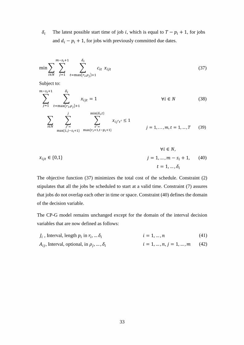
𝛿𝑖 The latest possible start time of job 𝑖, which is equal to 𝑇 − 𝑝𝑖 + 1, for jobs

and 𝑑𝑖 − 𝑝𝑖 + 1, for jobs with previously committed due dates.

min∑ ∑ ∑ 𝑐𝑖𝑡

𝛿𝑖

𝑡=max(𝑟𝑖,𝜌𝑗)+1

𝑥𝑖𝑗𝑡

𝑚−𝑠𝑖+1

𝑗=1𝑖∈𝑁

(37)

Subject to:

∑ ∑ 𝑥𝑖𝑗𝑡

𝛿𝑖

𝑡=max(𝑟𝑖,𝜌𝑗)+1

𝑚−𝑠𝑖+1

𝑗=1

= 1 ∀𝑖 ∈ 𝑁 (38)

∑ ∑ ∑ 𝑥𝑖𝑗′𝑡′ ≤ 1

min{𝛿𝑖,𝑡}

𝑡′=max{𝑟𝑖+1,𝑡−𝑝𝑖+1}

𝑗

𝑗′=max{1,𝑗−𝑠𝑖+1}

𝑖∈𝑁

𝑗 = 1, . . . , 𝑚, 𝑡 = 1,… , 𝑇 (39)

𝑥𝑖𝑗𝑡 ∈ {0,1}

∀𝑖 ∈ 𝑁,

𝑗 = 1,… ,𝑚 − 𝑠𝑖 + 1,

𝑡 = 1,… , 𝛿𝑖

(40)

The objective function (37) minimizes the total cost of the schedule. Constraint (2)

stipulates that all the jobs be scheduled to start at a valid time. Constraint (7) assures

that jobs do not overlap each other in time or space. Constraint (40) defines the domain

of the decision variable.

The CP-G model remains unchanged except for the domain of the interval decision

variables that are now defined as follows:

𝐽𝑖 , Interval, length 𝑝𝑖 in 𝑟𝑖, … 𝛿𝑖 𝑖 = 1, … , 𝑛 (41)

𝐴𝑖𝑗, Interval, optional, in 𝜌𝑗 , … , 𝛿𝑖 𝑖 = 1, … , 𝑛, 𝑗 = 1,… ,𝑚 (42)