Embed Size (px)
Citation preview
THE CONSTRUCTIVE SYSTEMS ENGINEERING COST MODEL (COSYSMO)
by
Ricardo Valerdi
A Dissertation Presented to the FACULTY OF THE GRADUATE SCHOOL
UNIVERSITY OF SOUTHERN CALIFORNIA In Partial Fulfillment of the
Requirements for the Degree DOCTOR OF PHILOSOPHY
(INDUSTRIAL AND SYSTEMS ENGINEERING)
August 2005
Copyright 2005 Ricardo Valerdi

ii
DEDICATION
This dissertation is dedicated to my mother and father, Lucía and Jorge.
iii
ACKNOWLEDGEMENTS
If I have been able to see further than others, it is because I have stood on the
shoulders of giants.
Sir Isaac Newton
No intellectual achievement occurs in a vacuum. All new creativity builds on the
efforts that have gone before. Like Newton, I have been able to stand on the shoulders of
extremely talented people. I am forever in debt to these giants which have contributed
intellectual ingredients to this work. First, my family for providing a strong foundation.
Second, my academic advisors and colleagues for exposing me to the world of
engineering. And third, the organizations that supported this research through funding,
expertise, and data.
My mother, Lucia, for teaching me values that have helped me become a member
of society and my father for teaching me how to use those values to make a contribution.
To my fiancée Briana for her unconditional support and unending patience.
The ideas presented here exist as a result of the trailblazing vision and persistence
of my advisor, Dr. Barry W. Boehm. Unconditional intellectual support was provided by
Dr. Stan Settles, Dr. George Friedman, Dr. Ann Majchrzak, Dr. Elliot Axelband, Dr. Bert
Steece and Don Reifer.
iv
The realization of this model exists because of the tremendous support of the
Center for Software Engineering corporate affiliates. Specifically, Gary Thomas from
Raytheon whose development of myCOSYSMO served as a catalyst for the acceptance of
the model among practitioner circles. Special thanks to Merrill Palmer, John Gaffney,
and Dan Ligett for thoroughly reviewing this manuscript. Others providing intellectual
support are listed in Appendix C.
I am grateful for the support of Marilee Wheaton and Pat Maloney from The
Aerospace Corporation. Additional support was provided by the Air Force Space and
Missile Systems Center, Office of the Chief Engineer. This research has also received
visibility and endorsement from: the International Council on Systems Engineering
(Corporate Advisory Board, Measurement Working Group, and Systems Engineering
Center of Excellence); Southern California Chapter of the International Society of
Parametric Analysts; Practical Software & Systems Measurement; and the Space Systems
Cost Analysis Group.
v
TABLE OF CONTENTS
DEDICATION.................................................................................................................... ii ACKNOWLEDGEMENTS............................................................................................... iii LIST OF TABLES............................................................................................................ vii LIST OF FIGURES ............................................................................................................ x ABREVIATIONS.............................................................................................................. xi ABSTRACT..................................................................................................................... xiii 1. Introduction................................................................................................................. 1
1.1. Motivation for a Systems Engineering Cost Model............................................ 1 1.1.1. Fundamentals of Systems Engineering........................................................... 2
1.1.2. Comparison Between COCOMO II and COSYSMO................................. 5 1.1.3. COSYSMO Objectives ............................................................................... 7
1.2. Systems Engineering and Industry Standards..................................................... 9 1.3. Proposition and Hypotheses.............................................................................. 14
2. Background and Related Work................................................................................. 17
2.1. State of the Practice .......................................................................................... 17 2.2. COSYSMO Lineage ......................................................................................... 22 2.3. Overview of Systems Engineering Estimation Methods .................................. 23
3. Model Definition....................................................................................................... 28
3.1. COSYSMO Derivation ..................................................................................... 28 3.1.1. Evolution................................................................................................... 28 3.1.2. Model Form .............................................................................................. 31
3.2. Systems Engineering Size Drivers.................................................................... 38 3.2.1. Number of System Requirements ............................................................. 42 3.2.2. Number of System Interfaces.................................................................... 48 3.2.3. Number of Algorithms.............................................................................. 50 3.2.4. Number of Operational Scenarios............................................................. 54
3.3. Systems Engineering Cost Drivers ................................................................... 56 3.3.1. Understanding Factors .............................................................................. 58 3.3.2. Complexity Factors................................................................................... 61 3.3.3. Operations Factors .................................................................................... 65 3.3.4. People Factors........................................................................................... 67 3.3.5. Environment Factors................................................................................. 69
vi
4. Methodology............................................................................................................. 72 4.1. Research Design & Data Collection ................................................................. 72 4.2. Threats to Validity & Limitations..................................................................... 82
5. Results and Next Steps.............................................................................................. 91 5.1. Delphi Results....................................................................................................... 91
5.2. Model Verification............................................................................................ 96 5.2.1. Statistical Tests ......................................................................................... 97 5.2.2. Model Parsimony .................................................................................... 101 5.2.3. Bayesian Approximation ........................................................................ 108 5.2.4. Stratification by Organization................................................................. 110
5.3. Conclusion ...................................................................................................... 112 5.3.1. Contributions to the Field of Systems Engineering ................................ 113 5.3.2. Areas for Future Work ............................................................................ 115
Appendix A: ANSI/EIA 632 Activities .......................................................................... 126 Appendix B: Systems Engineering Effort Profile........................................................... 127 Appendix C: List of Industry participants ...................................................................... 128 Appendix D: List of Data Sources .................................................................................. 129 Appendix E: Example Estimate Using COSYSMO ....................................................... 130 Appendix F: Cost Driver Correlation Matrix.................................................................. 131 Appendix G: Cost Driver Distributions .......................................................................... 132 Appendix H: Regression Results for Final Model.......................................................... 137
vii
LIST OF TABLES
Table 1 Collection of Definitions of Systems Engineering ................................................ 3 Table 2 Differences between COCOMO II and COSYSMO ............................................. 6 Table 3 Notable Systems Engineering Standards ............................................................... 9 Table 4 Cost Models With Systems Engineering Components ........................................ 19 Table 5 Size Drivers and Corresponding Data Items........................................................ 39 Table 6 Adjustment Factors for Size Drivers ................................................................... 42 Table 7 Number of System Requirements Definition....................................................... 43 Table 8 Number of System Requirements Rating Scale................................................... 43 Table 9 Number of System Interfaces Definition ............................................................. 48 Table 10 Number of System Interfaces Rating Scale ....................................................... 49 Table 11 Number of System-Specific Algorithms Definition .......................................... 50 Table 12 Number of System-Specific Algorithms Rating Scale ...................................... 50 Table 13 Candidate Entities and Attributes for Algorithms ............................................. 51 Table 14 Number of Operational Scenarios Definition .................................................... 54 Table 15 Number of Operational Scenarios Rating Scale ................................................ 54 Table 16 Cost Drivers and Corresponding Data Items ..................................................... 56 Table 17 Requirements Understanding Definition ........................................................... 59 Table 18 Requirements Understanding Rating Scale ....................................................... 59 Table 19 Architecture Understanding Definition ............................................................. 59 Table 20 Architecture Understanding Rating Scale.......................................................... 59 Table 21 Stakeholder Team Cohesion Definition............................................................. 60
viii
Table 22 Stakeholder Team Cohesion Rating Scale......................................................... 60 Table 23 Personnel Experience/Continuity Definition ..................................................... 61 Table 24 Personnel Experience/Continuity Rating Scale ................................................. 61 Table 25 Level of Service Requirements Definitions....................................................... 61 Table 26 Level of Service Requirements Rating Scale .................................................... 62 Table 27 Technology Risk Definition............................................................................... 62 Table 28 Technology Risk Rating Scale........................................................................... 63 Table 29 Number of Recursive Levels in the Design Definition...................................... 63 Table 30 Number of Recursive Levels in the Design Rating Scale.................................. 64 Table 31 Documentation Match to Life Cycle Needs Definition ..................................... 64 Table 32 Documentation Match to Life Cycle Needs Rating Scale ................................. 64 Table 33 Number and Diversity of Installations/Platforms Definition............................. 66 Table 34 Number and Diversity of Installations/Platforms Rating Scale......................... 66 Table 35 Migration Complexity Definition ...................................................................... 67 Table 36 Migration Complexity Rating Scale .................................................................. 67 Table 37 Personnel/Team Capability Definition .............................................................. 67 Table 38 Personnel/Team Capability Rating Scale .......................................................... 67 Table 39 Process Capability Definition ............................................................................ 68 Table 40 Process Capability Rating Scale ........................................................................ 68 Table 41 Multisite Coordination Definition ..................................................................... 69 Table 42 Multisite Coordination Rating Scale.................................................................. 70 Table 43 Tool Support Definition..................................................................................... 70

ix
Table 44 Tool Support Rating Scale................................................................................. 70 Table 45 Research Designs and Approaches Used........................................................... 77 Table 46 Consolidation of Aerospace Companies............................................................ 85 Table 47 COCOMO II and COSYSMO Overlaps............................................................ 90 Table 48 Relative Weights for Size Drivers from Delphi Round 3.................................. 92 Table 49 Rating Scale Values for Cost Drivers from Delphi Round 3............................. 93 Table 50 COSYSMO Predictor Descriptions ................................................................... 99 Table 51 Systems Engineering Effort Distribution % Across ISO/IEC 15288 Phases .. 103 Table 52 Comparison of Model Performance................................................................. 107 Table 53 Model Accuracy of Delphi Based Model ........................................................ 108 Table 54 Relative Weights for Size Drivers for Bayesian Calibrated Model................. 109 Table 55 Bayesian Calibrated Rating Scale Multipliers ................................................. 109 Table 56 Model Accuracy of Bayesian Calibrated Model.............................................. 110 Table 57 Model Accuracy by Organization.................................................................... 110
x
LIST OF FIGURES Figure 1 COSYSMO System Life Cycle Phases .............................................................. 11 Figure 2 Model Life Cycle Phases Compared .................................................................. 21 Figure 3 Notional Relationships Between Operational Scenarios.................................... 35 Figure 4 Examples of Diseconomies of Scale .................................................................. 37 Figure 5 Notional Example of Requirements Translation from Customer to Contractor. 44 Figure 6 Cockburn’s Hierarchy as Related to COSYSMO Use Case Levels................... 48 Figure 7 Effort Decomposition Associated With an Algorithm ....................................... 52 Figure 8 Operational Scenario Example ........................................................................... 55 Figure 9 Cost Driver Clustering........................................................................................ 58 Figure 10 Seven Step Modeling Methodology ................................................................. 76 Figure 11 Data Handshaking ............................................................................................ 82 Figure 12 Application Domains of Delphi Participants.................................................... 89 Figure 13 Relative Weights for Size Drivers from Delphi Round 3................................. 92 Figure 14 Cost Driver EMRs in Order of Influence from Delphi Round 3...................... 95 Figure 15 Size Versus Adjusted Systems Engineering Hours ........................................ 104 Figure 16 Productivity Histogram for 42 projects .......................................................... 105
xi
ABREVIATIONS
ANSI American National Standards Institute C4ISR Command Control Communications Computer Intelligence
Surveillance Reconnaissance CER Cost Estimation Relationship CM Configuration Management CMM Capability Maturity Model CMMI Capability Maturity Model Integration COCOMO II Constructive Cost Model version II COCOTS Constructive Commercial-off-the-shelf Model COPROMO Constructive Productivity Model COPSEMO Constructive Phased Schedule Estimation Model COQUALMO Constructive Quality Model CORADMO Constructive Rapid Application Development Model COSOSIMO Constructive System-of-systems Cost Model COSYSMO Constructive Systems Engineering Cost Model CSE Center for Software Engineering CSER Conference on Systems Engineering Research DCAA Defense Contract Audit Agency DF Degrees of Freedom DoD Department of Defense EIA Electronic Industries Alliance EM Effort Multiplier EMR Effort Multiplier Ratio GAO Government Accountability Office GUTSE Grand Unified Theory of Systems Engineering IEC International Electrotechnical Commission IEEE Institute of Electrical and Electronics Engineers IKIWISI I’ll Know It When I See It INCOSE International Council on Systems Engineering IP Information Processing ISO International Organization for Standardization KPA Key Process Area KPP Key Performance Parameter KSLOC Thousands of Software Lines of Code MBASE Model Based System Architecting and Software Engineering MIL-STD Military Standard MITRE MIT Research Corporation MMRE Mean Magnitude of Relative Error MSE Mean Square Error OLS Ordinary Least Squares OTS Off The Shelf PM Person Month
xii
PRED Prediction level PRICE Parametric Review of Information for Costing and Evaluation RSERFT Raytheon Systems Engineering Resource Forecasting Tool RSS Residual Sum of Squares RUP Rational Unified Process SE Systems Engineering SEER System Evaluation and Estimation of Resources SEMP Systems Engineering Management Plan SMC Space and Missile Systems Center SoS System-of-systems SSCM Small Satellite Cost Model SW Software TPM Technical Performance Measure TRL Technology Readiness Level USCM Unmanned Satellite Cost Model WBS Work Breakdown Structure
xiii
ABSTRACT
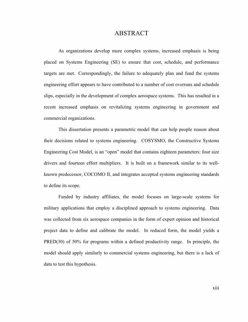
As organizations develop more complex systems, increased emphasis is being
placed on Systems Engineering (SE) to ensure that cost, schedule, and performance
targets are met. Correspondingly, the failure to adequately plan and fund the systems
engineering effort appears to have contributed to a number of cost overruns and schedule
slips, especially in the development of complex aerospace systems. This has resulted in a
recent increased emphasis on revitalizing systems engineering in government and
commercial organizations.
This dissertation presents a parametric model that can help people reason about
their decisions related to systems engineering. COSYSMO, the Constructive Systems
Engineering Cost Model, is an “open” model that contains eighteen parameters: four size
drivers and fourteen effort multipliers. It is built on a framework similar to its well-
known predecessor, COCOMO II, and integrates accepted systems engineering standards
to define its scope.
Funded by industry affiliates, the model focuses on large-scale systems for
military applications that employ a disciplined approach to systems engineering. Data
was collected from six aerospace companies in the form of expert opinion and historical
project data to define and calibrate the model. In reduced form, the model yields a
PRED(30) of 50% for programs within a defined productivity range. In principle, the
model should apply similarly to commercial systems engineering, but there is a lack of
data to test this hypothesis.
xiv
The ultimate contributions of this dissertation can be found in at least two major
areas: (a) in the theoretical and methodological domain of systems modeling in the quest
of a more quantitative cost estimation framework, and (b) in advancing the state of
practice in the assessment and tracking of systems engineering in the development of
large aerospace systems.
1
1. Introduction
1.1. Motivation for a Systems Engineering Cost Model
It is clear that we have been living in the Systems Age for some time as
evidenced by the role of technologically enabled systems in our every day lives.
Most of our every day functions are dependent on, or enabled by, large scale man
made systems that provide useful technological capabilities. The advent of these
systems has created the need for systems thinking and ultimately systems
engineering.
The function of systems engineering – coupled with the other traditional
disciplines such as electrical engineering, mechanical engineering, or civil
engineering – enables the creation and implementation of systems of unprecedented
size and complexity. However, these disciplines differ in the way they create value.
Traditional engineering disciplines are value-neutral; the laws of physics control the
outcome of electronics, mechanics, and structures. Tangible products serve as
evidence of the contribution that is easily quantifiable. Systems engineering has a
different paradigm in that its intellectual output is often intangible and more difficult
to quantify. Common work artifacts such as requirements, architecting, design,
verification, and validation are not readily noticed. For this reason, systems
engineering is better suited for value-based approach artifacts where value
considerations are integrated with systems engineering principles and practices. The
link between systems engineering artifacts to cost and schedule is recognized but
2
currently not well understood. This leads to the principal research question
addressed in this dissertation:
How much systems engineering effort, in terms of person months, should be
allocated for the successful conceptualization, development, and testing of
large-scale systems?
The model presented in this dissertation, COSYSMO, helps address this issue using
a value-based approach.
1.1.1. Fundamentals of Systems Engineering
Systems engineering is concerned with creating and executing an
interdisciplinary process to ensure that the customer and stakeholder needs are
satisfied in a high quality, trustworthy, cost efficient and schedule compliant manner
throughout a system's entire life cycle. Part of the complexity in understanding the
cost involved with systems engineering is due to the diversity of definitions used by
different systems engineers and the unique ways in which systems engineering is
used in practice. The premier systems engineering society, INCOSE, has long
debated the definition of systems engineering and only recently converged on the
following:
Systems Engineering is an interdisciplinary approach and means to enable the realization of successful systems. It focuses on defining customer needs and required functionality early in the development cycle, documenting requirements, then proceeding with design synthesis and system validation while considering the complete problem.
Experts have provided their own definitions of systems engineering as shown
in Table 1.
3
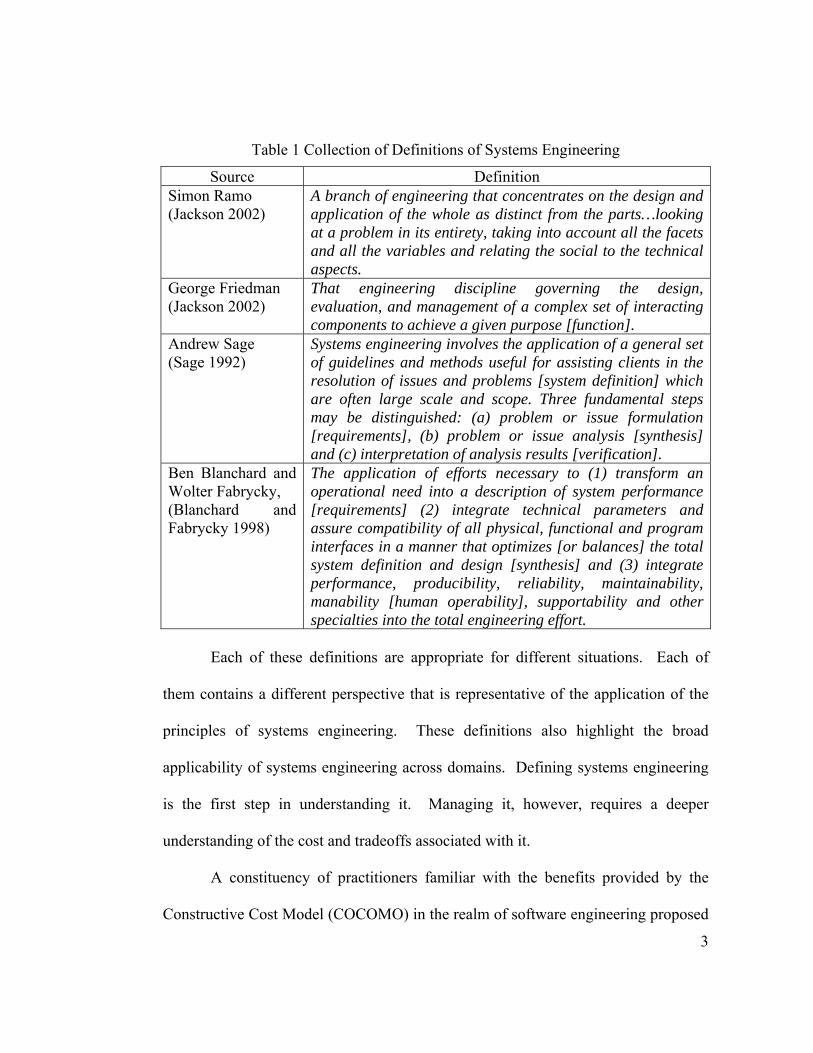
Table 1 Collection of Definitions of Systems Engineering
Source Definition Simon Ramo (Jackson 2002)
A branch of engineering that concentrates on the design and application of the whole as distinct from the parts…looking at a problem in its entirety, taking into account all the facets and all the variables and relating the social to the technical aspects.
George Friedman (Jackson 2002)
That engineering discipline governing the design, evaluation, and management of a complex set of interacting components to achieve a given purpose [function].
Andrew Sage (Sage 1992)
Systems engineering involves the application of a general set of guidelines and methods useful for assisting clients in the resolution of issues and problems [system definition] which are often large scale and scope. Three fundamental steps may be distinguished: (a) problem or issue formulation [requirements], (b) problem or issue analysis [synthesis] and (c) interpretation of analysis results [verification].
Ben Blanchard and Wolter Fabrycky, (Blanchard and Fabrycky 1998)
The application of efforts necessary to (1) transform an operational need into a description of system performance [requirements] (2) integrate technical parameters and assure compatibility of all physical, functional and program interfaces in a manner that optimizes [or balances] the total system definition and design [synthesis] and (3) integrate performance, producibility, reliability, maintainability, manability [human operability], supportability and other specialties into the total engineering effort.
Each of these definitions are appropriate for different situations. Each of
them contains a different perspective that is representative of the application of the
principles of systems engineering. These definitions also highlight the broad
applicability of systems engineering across domains. Defining systems engineering
is the first step in understanding it. Managing it, however, requires a deeper
understanding of the cost and tradeoffs associated with it.
A constituency of practitioners familiar with the benefits provided by the
Constructive Cost Model (COCOMO) in the realm of software engineering proposed
4
the development of a similar model to focus on systems engineering (Boehm, Egyed
et al. 1998). No formal approach to estimating systems engineering existed at the
time, partially because of the immaturity of systems engineering as a formal
discipline and the lack of mature metrics. The beginnings of systems engineering
can be traced back to the Bell Telephone Laboratories in the 1940s (Auyang 2004).
However, it was not until almost thirty years later that the first U.S. military standard
was published (MIL-STD-499A 1969). The first professional systems engineering
society, INCOSE, was not organized until the early 1990s and the first commercial
U.S. systems engineering standards, ANSI/EIA 632 and IEEE 1220, followed shortly
thereafter. Even with the different approaches of defining systems engineering, the
capability to estimate it is desperately needed by organizations. Several heuristics
are available but they do not provide the necessary level of detail that is required to
understand the most influential factors and their sensitivity to cost.
Fueled by industry support and the US Air Force’s systems engineering
revitalization initiative (Humel 2003), interest in COSYSMO has grown. Defense
contractors as well as the federal government are in need of a model that will help
them better control and prevent future shortfalls in the $18 billion federal space
acquisition process (GAO 2003). COSYSMO is also positioned to make immediate
impact on the way organizations – and other engineering disciplines – view systems
engineering.
Based on the previous support for COCOMO II, COSYSMO is positioned to
leverage off the existing body of knowledge developed by the software community.
The synergy between software engineering and systems engineering is intuitive
5
because of the strong linkages in their products and processes. Researchers
identified strong relationships between the two disciplines (Boehm, 1994),
opportunities for harmonization (Faisandier & Lake, 2004), and lessons learned
(Honour, 2004). There have also been strong movements towards convergence
between software and systems as reflected in two influential standards: ISO 15504
Information technology - Process assessment and the CMMI1. Organizations are
going as far as changing their names to reflect their commitment and interest in this
convergence. Some examples include the Software Productivity Consortium
becoming the Systems & Software Consortium and the Software Technology
Conference becoming the Software & Systems Technology Conference. Despite the
strong coupling between software and systems they remain very different activities
in terms of maturity, intellectual advancement, and influences regarding cost.
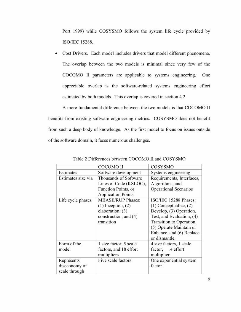
1.1.2. Comparison Between COCOMO II and COSYSMO
On the surface, COCOMO II and COSYSMO appear to be similar. However,
there are fundamental differences between them that should be highlighted. These
are obvious when the main assumptions of the model are considered:
• Sizing. COCOMO II uses software size metrics while COSYSMO uses
metrics at a level of the system that incorporates both hardware and software.
• Life cycle. COCOMO II, based on a software tradition, focuses exclusively
on software development life cycle phases defined by MBASE2 (Boehm and
1 Capability Maturity Model Integration 2 Model Based System Architecting and Software Engineering
6
Port 1999) while COSYSMO follows the system life cycle provided by
ISO/IEC 15288.
• Cost Drivers. Each model includes drivers that model different phenomena.
The overlap between the two models is minimal since very few of the
COCOMO II parameters are applicable to systems engineering. One
appreciable overlap is the software-related systems engineering effort
estimated by both models. This overlap is covered in section 4.2
A more fundamental difference between the two models is that COCOMO II
benefits from existing software engineering metrics. COSYSMO does not benefit
from such a deep body of knowledge. As the first model to focus on issues outside
of the software domain, it faces numerous challenges.
Table 2 Differences between COCOMO II and COSYSMO
COCOMO II COSYSMO Estimates Software development Systems engineering Estimates size via Thousands of Software
Lines of Code (KSLOC), Function Points, or Application Points
Requirements, Interfaces, Algorithms, and Operational Scenarios
Life cycle phases MBASE/RUP Phases: (1) Inception, (2) elaboration, (3) construction, and (4) transition
ISO/IEC 15288 Phases: (1) Conceptualize, (2) Develop, (3) Operation, Test, and Evaluation, (4) Transition to Operation, (5) Operate Maintain or Enhance, and (6) Replace or dismantle.
Form of the model
1 size factor, 5 scale factors, and 18 effort multipliers
4 size factors, 1 scale factor, 14 effort multiplier
Represents diseconomy of scale through
Five scale factors One exponential system factor
7
COCOMO II was a natural starting point which provided a useful and mature
framework. The scope of this dissertation is to identify the relevant parameters in
systems engineering while building from the lessons learned in software cost
estimation. As much synergy as exists, software engineering and systems
engineering must be treated as independent activities. This involves measuring them
independently and identifying metrics that best capture the size and cost factors for
each.
1.1.3. COSYSMO Objectives
COSYSMO is a model that can help people reason about the cost
implications of systems engineering. User objectives include the ability to make the
following:
• Investment decisions. A return-on-investment analysis involving a systems
engineering effort needs an estimate of the systems engineering cost or a life
cycle effort expenditure profile.
• Budget planning. Managers need tools to help them allocate project
resources.
• Tradeoffs. Decisions often need to be made between cost, schedule, and
performance.
• Risk management. Unavoidable uncertainties exist for many of the factors
that influence systems engineering.
8
• Strategy planning. Setting mixed investment strategies to improve an
organization’s systems engineering capability via reuse, tools, process
maturity, or other initiatives.
• Process improvement measurement. Investment in training and initiatives
often need to be measured. Quantitative management of these programs can
help monitor progress.
To enable these user objectives the model has been developed to provide
certain features to allow for decision support capabilities. Among these is to provide
a model that is:
• Accurate. Where estimates are close to the actual costs expended on the
project. See section 5.2.1.
• Tailorable. To enable ways for individual organizations to adjust the model
so that it reflects their business practices. See section 5.2.4.
• Simple. Understandable counting rules for the drivers and rating scales. See
section 3.2.
• Well-defined. Scope of included and excluded activities is clear. See
sections 3.2 and 3.3.
• Constructive. To a point that users can tell why the model gives the result it
does and helps them understand the systems engineering job to be done.
• Parsimonious. To avoid use of highly redundant factors or factors which
make no appreciable contribution to the results. See section 5.2.2.
• Pragmatic. Where inputs to the model correspond to the information
available early on in the project life cycle.
9
This research puts these objectives into context with the exploration of what
systems engineering means in practice. Industry standards are representative of
collective experiences that help shape the field as well as the scope of COSYSMO.
1.2. Systems Engineering and Industry Standards
The synergy between software engineering and systems engineering is
evident by the integration of the methods and processes developed by one discipline
into the culture of the other. Researchers from software engineering (Boehm 1994)
and systems engineering (Rechtin 1998) have extensively promoted the integration
of both disciplines but have faced roadblocks that result from the fundamental
difference between the two disciplines (Pandikow and Törne 2001).
The development of systems engineering standards has helped the
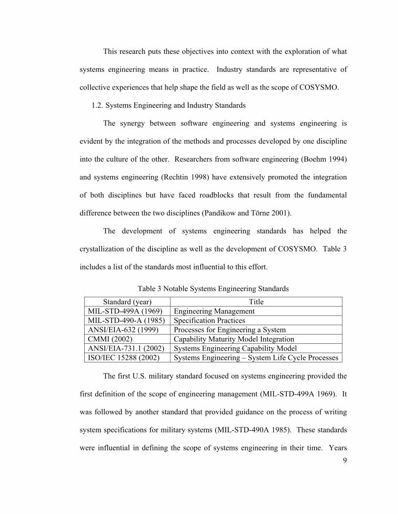
crystallization of the discipline as well as the development of COSYSMO. Table 3
includes a list of the standards most influential to this effort.
Table 3 Notable Systems Engineering Standards
Standard (year) Title MIL-STD-499A (1969) Engineering Management MIL-STD-490-A (1985) Specification Practices ANSI/EIA-632 (1999) Processes for Engineering a System CMMI (2002) Capability Maturity Model Integration ANSI/EIA-731.1 (2002) Systems Engineering Capability Model ISO/IEC 15288 (2002) Systems Engineering – System Life Cycle Processes
The first U.S. military standard focused on systems engineering provided the
first definition of the scope of engineering management (MIL-STD-499A 1969). It
was followed by another standard that provided guidance on the process of writing
system specifications for military systems (MIL-STD-490A 1985). These standards
were influential in defining the scope of systems engineering in their time. Years
10
later the standard ANSI/EIA 632 Processes for Engineering a System (ANSI/EIA
1999) provided a typical systems engineering WBS3. This list of activities was
selected as the baseline for defining systems engineering in COSYSMO. The
standard contains five fundamental processes and 13 high level process categories
that are representative of systems engineering organizations. The process categories
are further divided into 33 activities shown in Appendix A. These activities help
answer the what of systems engineering and helped characterize the first significant
deviation from the software domain covered by COCOMO II. The five fundamental
processes are (1) Acquisition and Supply, (2) Technical Management, (3) System
Design, (4) Product Realization, and (5) Technical Evaluation. These processes are
the basis of the systems engineering effort profile developed for COSYSMO. The
effort profile is provided in Appendix B.
This standard provides a generic industry list which may not be applicable to
every situation. Other types of systems engineering WBS lists exist such as the one
developed by Raytheon Space & Airborne Systems (Ernstoff and Vincenzini 1999).
Lists such as this one provide, in much finer detail, the common activities that are
likely to be performed by systems engineers in those organizations, but are generally
not applicable outside of the companies or application domains in which they are
created.
Under the integrated software engineering and systems engineering paradigm,
or Capability Maturity Model Integration® (CMMI 2002), software and systems are
intertwined. A project’s requirements, architecture, and process are collaboratively
3 Work Breakdown Structure
11
developed by integrated teams based on shared vision and negotiated stakeholder
concurrence. A close examination of CMMI process areas – particularly the staged
representation – strongly suggests the need for the systems engineering function to
estimate systems engineering effort and cost as early as CMMI Maturity Level 2.
Estimates can be based upon a consistently provided organizational approach from
past project performance measures related to size, effort and complexity. While it
might be possible to achieve high CMMI levels without a parametric model, an
organization should consider the effectiveness and cost of achieving them using
other methods that may not provide the same level of stakeholder confidence and
predictability. The more mature an organization, the more benefits in productivity
they experience (ANSI/EIA 2002).
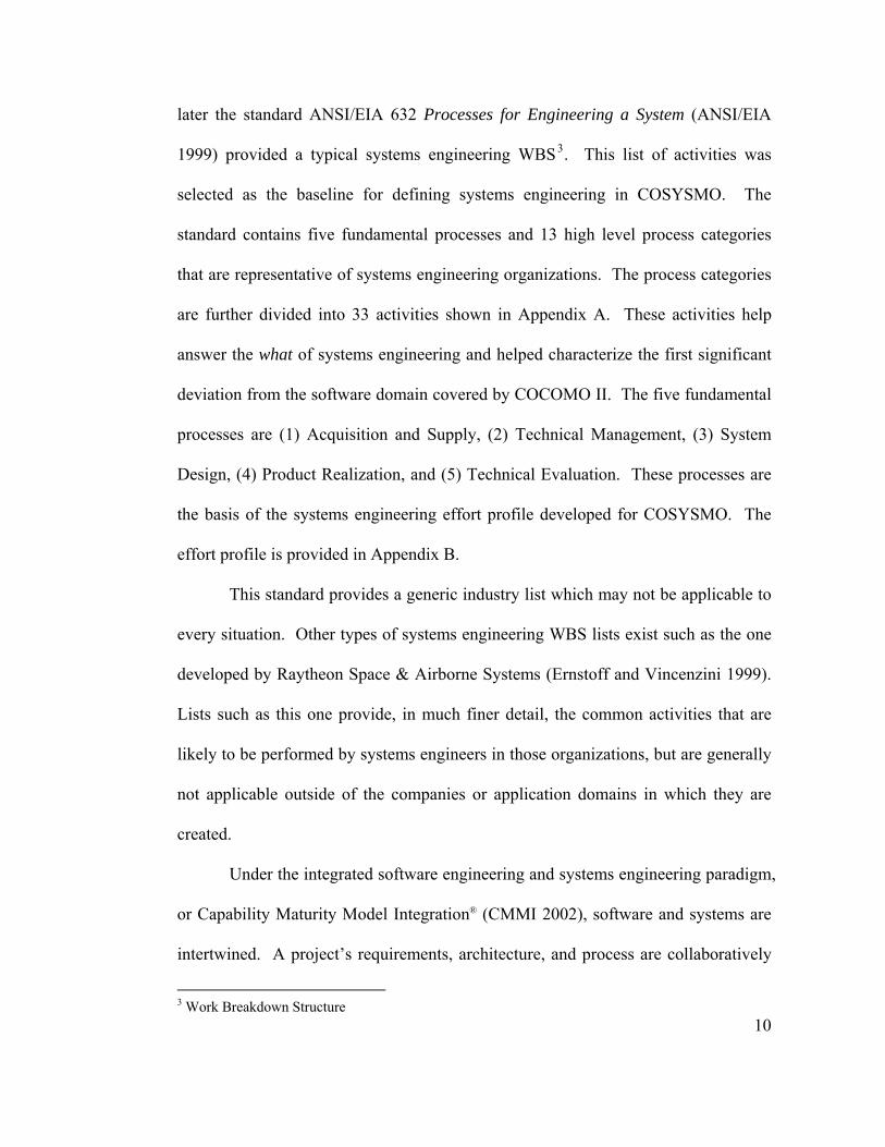
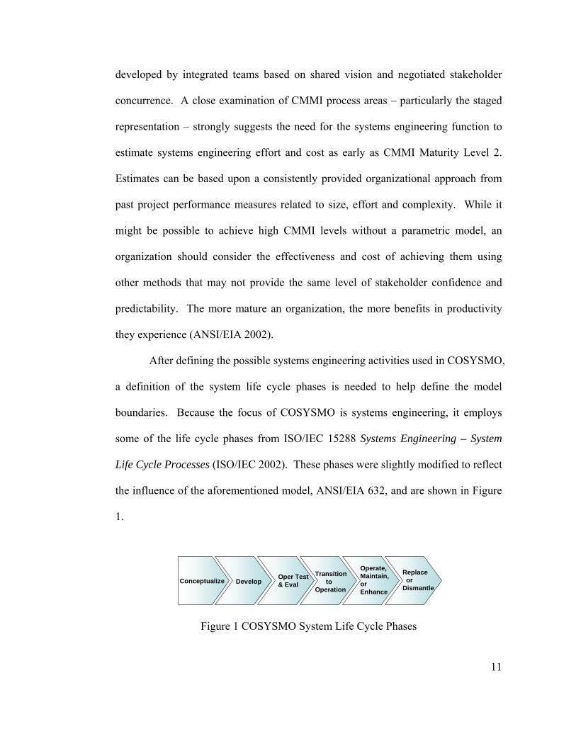
After defining the possible systems engineering activities used in COSYSMO,
a definition of the system life cycle phases is needed to help define the model
boundaries. Because the focus of COSYSMO is systems engineering, it employs
some of the life cycle phases from ISO/IEC 15288 Systems Engineering – System
Life Cycle Processes (ISO/IEC 2002). These phases were slightly modified to reflect
the influence of the aforementioned model, ANSI/EIA 632, and are shown in Figure
1.
Conceptualize DevelopOper Test & Eval
Transition to
Operation
Operate, Maintain, or Enhance
Replace or
Dismantle
Figure 1 COSYSMO System Life Cycle Phases
12
Life cycle models vary according to the nature, purpose, use and prevailing
circumstances of the system. Despite an infinite variety in system life cycle models,
there is an essential set of characteristic life cycle phases that exists for use in the
systems engineering domain. For example, the Conceptualize stage focuses on
identifying stakeholder needs, exploring different solution concepts, and proposing
candidate solutions. The Development stage involves refining the system
requirements, creating a solution description, and building a system. The
Operational Test & Evaluation stage involves verifying/validating the system and
performing the appropriate inspections before it is delivered to the user. The
Transition to Operation stage involves the transition to utilization of the system to
satisfy the users’ needs. These four life cycle phases are within the scope of
COSYSMO. The final two were included in the data collection effort but did not
yield enough data to perform a calibration. These phases are: Operate, Maintain, or
Enhance which involves the actual operation and maintenance of the system required
to sustain system capability, and Replace or Dismantle which involves the retirement,
storage, or disposal of the system.
Each stage has a distinct purpose and contribution to the whole life cycle and
represents the major life cycle periods associated with a system. The stages also
describe the major progress and achievement milestones of the system through its
life cycle. These life cycle stages help answer the when of systems engineering and
COSYSMO. Understanding when systems engineering is performed relative to the
system life cycle helps define anchor points for the model.
13
System-of-Interest. The ISO/IEC 15288 standard also provides a structure
that helps define the system hierarchy. Systems can be characterized by their
architectural structure or levels of responsibility. Each project has the responsibility
for using levels of system composition beneath it and creating an aggregate system
that meets the customer’s requirements. Each particular subproject views its system
as a system-of-interest within the grand scheme. The subproject’s only task may be
to deliver their system-of-interest to a higher level in the hierarchy. The top level of
the hierarchy is then responsible for integrating the subcomponents that are delivered
and providing a functional system. Essential services or functionalities are required
from the systems that make up the system hierarchy. These systems, called enabling
systems, can be made by the organization itself or purchased from other
organizations.
The system-of-interest framework helps answer the where of systems
engineering for use in COSYSMO. In the case where systems engineering takes
place at different levels of the hierarchy, organizations should focus on the portion of
the system which they are responsible for testing. Identifying system test
responsibility helps crystallize the scope of the systems engineering estimate at a
specific level of the system hierarchy.
The diversity of systems engineering standards can be quite complex (Sheard
1997), therefore only the applicable standards have been mentioned here. With the
need and general context for the model defined, the central proposition and
hypotheses for this research are proposed.
14
1.3. Proposition and Hypotheses
Clear definitions of the what, when, and where of systems engineering sets
the stage for the statement of purpose for COSYSMO. The central proposition at the
core of this research is:
There exists a subset of systems engineering projects for which it is possible
to create a parametric model that will estimate systems engineering effort
(a) for specific life cycle phases
(b) at a certain level of system decomposition
(c) with the same statistical criteria as the COCOMO suite of models at a
comparable stage of maturity in time and effort
This statement provides the underlying goal of the model by clarifying its
solution space. The selection of the subset of systems engineering projects attempts
to provide a homogenous group of projects from which the model can be based. For
the COSYSMO data set, useful discriminators included: systems engineering
productivity, systems engineering domain, and organization providing the data. The
term parametric implies that a given equation represents a mean function that is
characteristic of Cost Estimating Relationships in systems engineering. Specific life
cycle phases are selected based on the data provided by industry participants.
Counting rules are provided for a level of system decomposition to ensure uniform
counting rules across organizations that use the model. Similar statistical criteria are
used to evaluate COSYSMO for comparison with other cost estimation models.
The central proposition was validated through the use of the scientific method
(Isaac and Michael 1997) and analysis of data (Cook and Weisberg 1999) with the
15
aim of developing a meaningful solution. In terms of scientific inquiry, the model
was validated through the following hypotheses:
H#1: A combination of the four elements of functional size in COSYSMO
contributes significantly to the accurate estimation of systems engineering
effort.
The criteria used was a significance level less than or equal to 0.10 which
translates to a 90% confidence level that these elements are significant.
H#2: An ensemble of COSYSMO effort multipliers contribute significantly to
the accurate estimation of systems engineering.
The same significance level of 0.10 was used to test this hypothesis.
H#3: The value of the COSYSMO exponent, E, which can represent
economies/diseconomies of scale is greater than 1.0.
To test this hypothesis, different values for E were calculated and their effects
were tested on model accuracy.
H#4: There exists a subset of systems engineering projects for which it is
possible to create a parametric model that will estimate systems engineering effort at
a PRED(30) accuracy of 50%.
Various approaches were used to fine tune the model and bring to a point
where it was possible to test this hypothesis.
Each hypothesis is designed to test key assumptions of the model. These
assumptions, as well as the structure of the model, are discussed in more detail in the
next section. In addition to the four quantitative hypotheses, a qualitative hypothesis
was developed to test the impact of the model on organizations.
16
H#5: COSYSMO makes organizations think differently about Systems
Engineering cost.
The hypothesis was validated through interviews with engineers from the
participating companies that provided historical data and expert opinion in the
Delphi survey.
17
2. Background and Related Work
2.1. State of the Practice
The origins of parametric cost estimating date back to World War II (NASA
2002). The war caused a demand for military aircraft in numbers and models that far
exceeded anything the aircraft industry had manufactured before. While there had
been some rudimentary work to develop parametric techniques for predicting cost,
there was no widespread use of any cost estimating technique beyond a bottoms-up
buildup of labor-hours and materials. A type of statistical estimating was suggested
in 1936 by T. P. Wright in the Journal of Aeronautical Science. Wright provided
equations which could be used to predict the cost of airplanes over long production
runs, a theory which came to be called the learning curve. By the time the demand
for airplanes had exploded in the early years of World War II, industrial engineers
were using Wright's learning curve to predict the unit cost of airplanes. Today,
parametric cost models are used for estimating software development (Boehm, Abts
et al. 2000), unmanned satellites (USCM 2002), and hardware development (PRICE-
H 2002).
A parametric cost model is defined as: a group of cost estimating
relationships used together to estimate entire cost proposals or significant portions
thereof. These models are often computerized and may include many interrelated
Cost Estimation Relationships (CERs), both cost-to-cost and cost-to-non-cost. The
use of parametric models in engineering management serves as valuable tools for
engineers and project managers to estimate engineering effort. Developing these
18
estimates requires a strong understanding of the factors that affect, in this case,
systems engineering effort.
An important part of developing a model such as COSYSMO is recognizing
previous work in related areas. This process often provides a stronger case for the
existence of the model and ensures that its capabilities and limitations are clearly
defined. This section provides an overview of an analysis done on eight existing cost
models - three of which focus on software and five on hardware (Valerdi, Ernstoff et
al. 2003). These models include SE components and each employs its own unique
approaches to sizing systems. An overview of the genesis and assumptions of each
model sheds light on their individual applicability. While it has been shown that the
appropriate level of SE effort leads to better control of project costs (Honour 2002),
identifying the necessary level of SE effort is not yet a mature process. Some
projects use the traditional 15% of the prime mission product or prime mission
equipment to estimate systems engineering, while other projects tend to use informal
rules of thumb. These simplified and inaccurate methods can lead to excessively
high bids by allocating too many hours on SE or, even worse, may underestimate the
amount of SE needed.
One significant finding during the review was that SE costs were extremely
sensitive to the sizing rules that formed the basis of these models. These rules help
estimators determine the functional size of systems and, by association, the size of
the job. Similar comparative analysis of cost models has been completed (Kemerer
1987), which focused exclusively on models for software development. Going one
19
step further, both software and hardware cost models are considered since they are
both tightly coupled with SE.
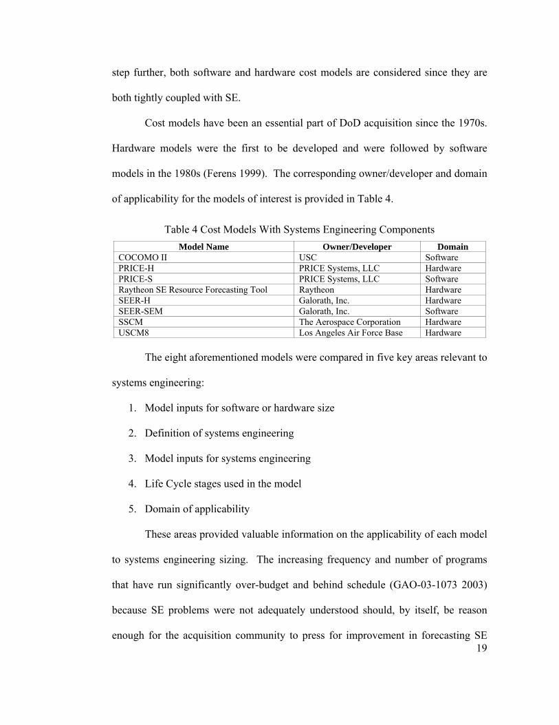
Cost models have been an essential part of DoD acquisition since the 1970s.
Hardware models were the first to be developed and were followed by software
models in the 1980s (Ferens 1999). The corresponding owner/developer and domain
of applicability for the models of interest is provided in Table 4.
Table 4 Cost Models With Systems Engineering Components
Model Name Owner/Developer Domain COCOMO II USC Software PRICE-H PRICE Systems, LLC Hardware PRICE-S PRICE Systems, LLC Software Raytheon SE Resource Forecasting Tool Raytheon Hardware SEER-H Galorath, Inc. Hardware SEER-SEM Galorath, Inc. Software SSCM The Aerospace Corporation Hardware USCM8 Los Angeles Air Force Base Hardware
The eight aforementioned models were compared in five key areas relevant to
systems engineering:
1. Model inputs for software or hardware size
2. Definition of systems engineering
3. Model inputs for systems engineering
4. Life Cycle stages used in the model
5. Domain of applicability
These areas provided valuable information on the applicability of each model
to systems engineering sizing. The increasing frequency and number of programs
that have run significantly over-budget and behind schedule (GAO-03-1073 2003)
because SE problems were not adequately understood should, by itself, be reason
enough for the acquisition community to press for improvement in forecasting SE
20
resource needs. However, even if the history of SE problems is ignored, the future
paints an even more demanding picture. The undeniable trend is toward increasingly
complex systems dependent on the coordination of interdisciplinary developments
where effective system engineering is no longer just another technology, but the key
to getting the pieces to fit together. It is known that increasing front-end analysis
reduces the probability of problems later on, but excessive front-end analysis may
not pay the anticipated dividends. The key is to accurately estimate early in a
program the appropriate level of SE in order to ensure system success within cost
and schedule budgets.
Most widely used estimation tools, shown in Table 4, treat SE as a subset of a
software or a hardware effort. Since complex systems are not dominated by either
hardware or software, SE ought not to be viewed as a subset of hardware or software.
Rather, because many functions can be implemented using either hardware or
software, SE is becoming the discipline for selecting, specifying and coordinating the
various hardware and software designs. Given that role, the correct path is to
forecast SE resource needs based on the tasks that systems engineering must perform
and not as an arbitrary percentage of another effort. Hence, SE estimation tools must
provide for aligning the definition of tasks that SE is expected to do on a given
project with the program management's vision of economic and schedule cost,
performance, and risk.
Tools that forecast SE resources largely ignore factors that reflect the scope
of the SE effort, as insufficient historical data exists from which statistically
significant algorithms can be derived. To derive cost-estimating relationships from
21
historical data using regression analysis, one must have considerably more data
points than variables; such as a ratio of 5 to 1. It is difficult to obtain actual data on
systems engineering costs and on factors that impact those costs. For example, a
typical factor may be an aggressive schedule, which will increase the demand for SE
resources. The result is a tool set that inadequately characterizes the proposed
program and therefore inaccurately forecasts SE resource needs. Moreover, the tools
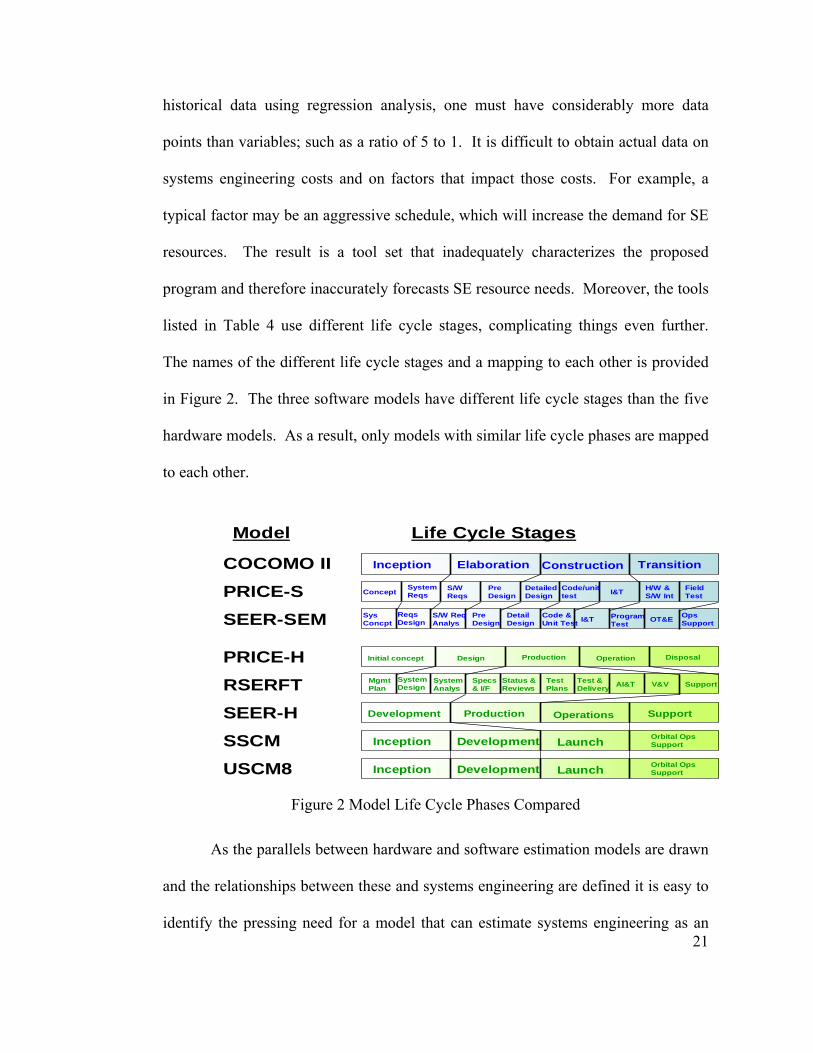
listed in Table 4 use different life cycle stages, complicating things even further.
The names of the different life cycle stages and a mapping to each other is provided
in Figure 2. The three software models have different life cycle stages than the five
hardware models. As a result, only models with similar life cycle phases are mapped
to each other.
Figure 2 Model Life Cycle Phases Compared
As the parallels between hardware and software estimation models are drawn
and the relationships between these and systems engineering are defined it is easy to
identify the pressing need for a model that can estimate systems engineering as an
Model Life Cycle Stages
COCOMO II
PRICE-S
SEER-SEM
PRICE-H
RSERFT
SEER-H
SSCM
USCM8
Inception Elaboration Construction Transition
Initial concept Design Production Operation
Development Production Operations Support
Inception Development Launch
Disposal
ConceptSystem Reqs
S/W Reqs
Pre Design
Detailed Design
Code/unittest I&T H/W &
S/W IntFieldTest
MgmtPlan
System Design
Specs& I/F
Status &Reviews
TestPlans AI&T V&V SupportSystem
AnalysTest &Delivery
SysConcpt
ReqsDesign
PreDesign
DetailDesign I&T Program
TestOT&ES/W Req
AnalysCode &Unit Test
OpsSupport
Orbital Ops Support
Inception Development Launch Orbital Ops Support
22
independent function. The fundamental approach for developing a model that meets
this demand relates back to the area of software cost estimation from which the
theoretical underpinnings of COSYSMO are derived. This area of research is
described in the next section.
2.2. COSYSMO Lineage
In order to place COSYSMO in the right context it must be linked to the
work that has preceded it. A wealth of models and processes exist in the area of
software engineering, from which this work is derived. Particularly the Model-
Based System Architecting and Software Engineering (MBASE) framework (Boehm
and Port 1999) developed for the purposes of tailoring a software project’s balance
of discipline and flexibility via risk considerations. As an elaboration of the spiral
model (Boehm and Hansen 2001), MBASE provides a framework for projects to use
various process, product, property, and success models. Process models include the
waterfall model, evolutionary development, incremental development, spiral
development, rapid application development, and many others. Product models
include various ways of specifying operational concepts, requirements, architectures,
designs, and code, along with their interrelationships. Property models include
models for cost, schedule, performance, reliability, security, portability, etc., and
their tradeoffs. Success models include organization and project goals, stakeholder
win-win, business-case, or IKIWISI (I’ll know it when I see it). COSYSMO is
considered a property model because it focuses on the effort and cost associated with
systems engineering and the tradeoffs between decisions that affect systems
engineering. Awareness of COSYSMO’s model category can help prevent clashes
23
between other models within or outside of the model category (Boehm and Port
1999). Equally important as COSYSMO’s lineage is its link to existing systems
engineering estimation methods. It provides valuable context of the state of the
practice surrounding it while informing users of the available alternatives.
2.3. Overview of Systems Engineering Estimation Methods
A number of useful systems engineering estimation techniques are currently
in use by practitioners. They vary in both maturity and sophistication. Subsequently,
some are more easily adaptable to the changing environment and others take more
time to develop. The logic behind these approaches is fundamentally different,
leaving only their results as measures of merit. It is believed that a hybrid approach
that borrows from each method is the best way to capture systems engineering
phenomena that a single approach may miss. Six estimation techniques are
presented here in order of sophistication.
Heuristics & rules of thumb. Heuristic reasoning has been commonly used
by engineers to arrive at quick answers to their questions. Practicing engineers,
through education, experience, and examples, accumulate a considerable body of
contextual intuition. These experiences evolve into instinct or common sense that
are seldom recorded. These can be considered insights, lessons learned, and rules of
thumb, among other names, that are brought to bear on certain situations. Ultimately,
this knowledge is based on experience and often provides valuable results. Systems
engineering cost estimation heuristics and rules of thumb have been developed by
researchers and practitioners (Boehm, Abts et al. 2000; Honour 2002; Rechtin 1991).
One such rule of thumb, provided by Barry Horowitz, retired CEO of MITRE
24
Corporation, adopts the following logic for estimating systems engineering effort
(Horowitz 2004):
If it is a custom developed system (mostly) or an Off-the-Shelf (OTS)
integration (mostly)
Then the former gets 6-15% of the total budget for SE, the later gets
15-25% of budget (where selection of OTS products as well as
standards is considered SE).
The following additional rules apply:
If the system unprecedented
Then raise the budget from minimum level to 50% more
If the system faces an extreme requirement (safety, performance, etc)
Then raise the budget by 25% of minimum
If the system involves a large number of distinct technologies, and
therefore a diversity of engineering disciplines and specialties
Then raise the budget by 25% of minimum
If the priority for the system is very high compared to other systems also
competing for resources
Then add 50% to the base
Note that the % of SE is larger for OTS, but since the budgets for these
projects are much lower, so are the numbers for SE.
Expert opinion. This is the most informal of the approaches because it
simply involves querying the experts in a specific domain and taking their subjective
25
opinion as an input. This approach is useful in the absence of empirical data and is
very simple. The obvious drawback is that an estimate is only as good as the
expert’s opinion, which can vary greatly from person to person. However, many
years of experience is not a guarantee of future expertise due to new requirements,
business processes, and added complexity. Moreover, this technique relies on
experts and even the most highly competent experts can be wrong. A common
technique for capturing expert opinion is the Delphi (Dalkey 1969) method which
was improved and renamed Wideband Delphi (Boehm 1981). This dissertation
employs the Wideband Delphi method which is elaborated in section 5.1.
Case studies and analogy. Recognizing that companies do not constantly
reinvent the wheel every time a new project comes along, there is an approach that
capitalizes on the institutional memory of an organization to develop its estimates.
Case studies represent an inductive process, whereby estimators and planners try to
learn useful general lessons by extrapolation from specific examples. They examine
in detail elaborate studies describing the environmental conditions and constraints
that were present during the development of previous projects, the technical and
managerial decisions that were made, and the final successes or failures that resulted.
They then determine the underlying links between cause and effect that can be
applied in other contexts. Ideally, they look for cases describing projects similar to
the project for which they will be attempting to develop estimates and apply the rule
of analogy that assumes previous performance is an indicator of future performance.
The sources of case studies may be either internal or external to the estimator’s own
organization. Homegrown cases are likely to be more useful for the purposes of
26
estimation because they reflect the specific engineering and business practices likely
to be applied to an organization’s projects in the future. Well-documented cases
studies from other organizations doing similar kinds of work can also prove very
useful so long as their differences are identified.
Top Down & Design To Cost. This technique aims for an aggregate
estimate for the cost of the project based upon the overall features of the system.
Once a total cost is estimated, each subcomponent is assigned a percentage of that
cost. The main advantage of this approach is the ability to capture system level
effort such as component integration and configuration management. It can also be
useful when a certain cost target must be reached regardless of the technical features.
The top down approach can often miss the low level nuances that can emerge in
large systems. It also lacks detailed breakdown of the subcomponents that make up
the system.
Bottom Up & Activity Based. Opposite the top-down approach, bottom-up
begins with the lowest level cost component and rolls it up to the highest level for its
estimate. The main advantage is that the lower level estimates are typically provided
by the people who will be responsible for doing the work. This work is typically
represented in the form of a Work Breakdown Structure (WBS), which makes this
estimate easily justifiable because of its close relationship to the activities required
by the project elements. This can translate to a fairly accurate estimate at the lower
level. The disadvantages are that this process is labor intensive and is typically not
uniform across entities. In addition, every level folds in another layer of
conservative management reserve which can result in an over estimate at the end.
27
Parametric cost estimation models. This method is the most sophisticated
and most difficult to develop. Parametric models generate cost estimates based on
mathematical relationships between independent variables (i.e., requirements) and
dependent variables (i.e., effort). The inputs characterize the nature of the work to
be done, plus the environmental conditions under which the work will be performed
and delivered. The definition of the mathematical relationships between the
independent and dependent variables is the heart of parametric modeling. These
relationships are commonly referred to Cost Estimating Relationships (CERs) and
are usually based upon statistical analyses of large amounts of data. Regression
models are used to validate the CERs and operationalize them in linear or nonlinear
equations. The main advantage of using parametric models is that, once validated,
they are fast and easy to use. They do not require a lot of information and can
provide fairly accurate estimates. Parametric models can also be tailored to a
specific organization’s CERs. The major disadvantage of parametric models is that
they are difficult and time consuming to develop and require a lot of clean, complete,
and uncorrelated data to be properly validated.
As a parametric model, COSYSMO contains its own CERs and is structured
in a way to accommodate the current systems engineering standards and processes.
Its structure is described in detail in the next section.
28
3. Model Definition
3.1. COSYSMO Derivation
Since its inception, COSYSMO has gone through three major iterations. This
section describes each of these spirals and the properties of the model at those points
in time culminating with the final form of the model represented in Equation 6.
3.1.1. Evolution
Spiral #1: Strawman COSYSMO. The first version of COSYSMO
contained a list of 16 systems engineering cost drivers. This representation of the
model was referred to as the “strawman” version because it provided a skeleton for
the model with limited content. The factors identified were ranked by relative
importance by a group of experts. Half of the factors were labeled application
factors and the other half were labeled team factors. Each parameter was determined
to have a high, medium, or low influence level on systems engineering cost. The
most influential application factor was requirements understanding and the most
influential team factor was personnel experience.
Function points and use cases were identified as possible measures of
systems engineering functional size. Factors for volatility and reuse were also
identified as relevant. At one point the initial list of parameters grew to as many as
24 during one of the brain storming sessions. For reasons related to model
parsimony, the number of parameters in the model was eventually reduced from 24
to 18.
29
Spiral #2: COSYSMO-IP. The second major version of COSYSMO
included refined definitions and a revised set of cost drivers. Most importantly, it
included measures for functional size that were independent of the software size
measures used in COCOMO II. This version had the letters “IP” attached to the end
to reflect the emphasis on software “Information Processing” systems as the initial
scope. Rooted from interest from industry stakeholders, the focus at the time was to
estimate systems engineering effort for software intensive systems. Moreover, this
version only covered the early phases of the life cycle: Conceptualize, Develop, and
Operational Test & Evaluation. Recognizing that the model had to evolve out of the
software intensive arena and on to a broader category of systems, a model evolution
plan was developed to characterize the different types of systems that could
eventually be estimated with COSYSMO and their corresponding life cycle stages
(Boehm, Reifer et al. 2003).
The important distinction between size drivers and cost drivers was also
clarified. At this stage, a general form for the model was proposed containing three
different types of parameters: additive, multiplicative, and exponential.
30
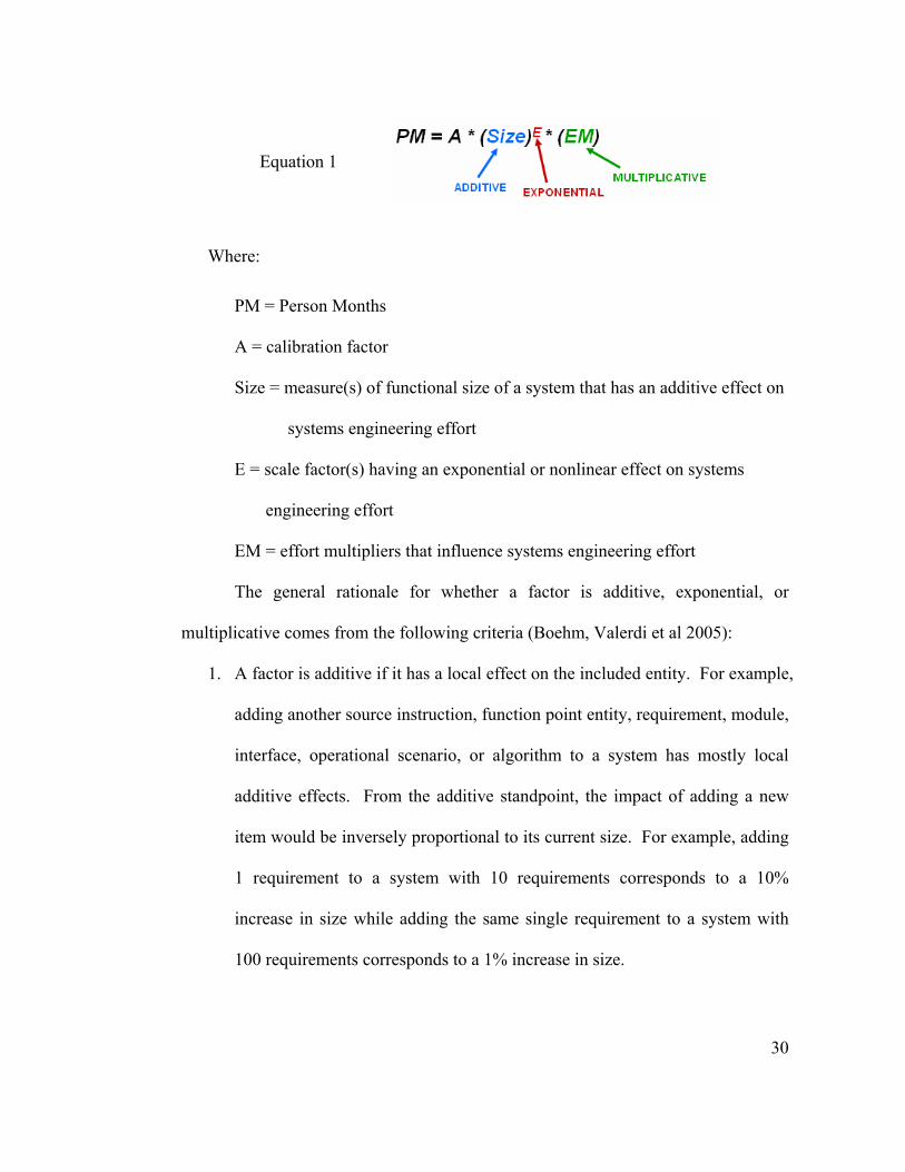
Equation 1
Where:
PM = Person Months
A = calibration factor
Size = measure(s) of functional size of a system that has an additive effect on
systems engineering effort
E = scale factor(s) having an exponential or nonlinear effect on systems
engineering effort
EM = effort multipliers that influence systems engineering effort
The general rationale for whether a factor is additive, exponential, or
multiplicative comes from the following criteria (Boehm, Valerdi et al 2005):
1. A factor is additive if it has a local effect on the included entity. For example,
adding another source instruction, function point entity, requirement, module,
interface, operational scenario, or algorithm to a system has mostly local
additive effects. From the additive standpoint, the impact of adding a new
item would be inversely proportional to its current size. For example, adding
1 requirement to a system with 10 requirements corresponds to a 10%
increase in size while adding the same single requirement to a system with
100 requirements corresponds to a 1% increase in size.
31
2. A factor is multiplicative if it has a global effect across the overall system.
For example, adding another level of service requirement, development site,
or incompatible customer has mostly global multiplicative effects. Consider
the effect of the factor on the effort associated with the product being
developed. If the size of the product is doubled and the proportional effect of
that factor is also doubled, then it is a multiplicative factor. For example,
introducing a high security requirement to a system with 10 requirements
would translate to a 40% increase in effort. Similarly, a high security
requirement for a system with 100 requirements would also increase by 40%.
3. A factor that is exponential has both a global effect and an emergent effect
for larger systems. If the effect of the factor is more influential as a function
of size because of the amount of rework due to architecture, risk resolution,
team compatibility, or readiness for SoS integration, then it is treated as an
exponential factor.
These statements are pivotal to the hypotheses stated in section 1.3. The next
section describes the form of the model and how the hypotheses are tested.
3.1.2. Model Form
Spiral #3: COSYSMO. Substantial insight was obtained from the
development of the first two iterations of the model. The current version, referred to
simply as COSYSMO, has a broader scope representative of the extensive
participation from industrial affiliates and INCOSE. Limiting the boundaries and
scope of the model has been one of the most challenging tasks to date, partially
32
because of the features desired by the large number of stakeholders involved in the
model development process.
The current operational form of the COSYSMO model is shown in Equation
2. As previously noted, the size drivers and cost drivers were determined via a
Delphi exercise by a group of experts in the fields of systems engineering, software
engineering, and cost estimation. The definitions for each of the drivers, while not
final, attempt to cover those activities that have the greatest impact on estimated
systems engineering effort and duration.
33
Equation 2 i
n
i
ENS EMSizeAPM
1)(
=Π⋅⋅=
Where:
PMNS = effort in Person Months (Nominal Schedule)
A = calibration constant derived from historical project data
Size = determined by computing the weighted sum of the four size drivers
E = represents economy/diseconomy of scale; default is 1.0
n = number of cost drivers (14)
EMi = effort multiplier for the ith cost driver. Nominal is 1.0. Adjacent
multipliers have constant ratios (geometric progression). Within their
respective rating scale, the calibrated sensitivity range of a multiplier is the
ratio of highest to lowest value.
Each parameter in the equation represents the Cost Estimating Relationships
(CERs) that were defined by systems engineering experts. The Size factor represents
the additive part of the model while the EM factor represents the multiplicative part
of the model. Specific definitions for these parameters are provided in the following
sections.
A detailed derivation of the terms in Equation 2 and motivation for the model
is provided here. The dependent variable is the number of systems engineering
person months of effort required under the assumption of a nominal schedule, or
PMNS. COSYSMO is designed to estimate the number of person months as a
function of a system’s functional size with considerations of diseconomies of scale.
34
Namely, larger systems will require proportionally more systems engineering effort
than smaller systems. That is, larger systems require a larger number of systems
engineering person months to complete. The four metrics selected as reliable
systems engineering size drivers are: Number of System Requirements, Number of
Major Interfaces, Number of Critical Algorithms, and Number of Operational
Scenarios. The weighted sum of these drivers represents a system’s functional size
from the systems engineering standpoint and is represented in the following CER:
Equation 3 ∑ Φ+Φ+Φ=k
ddnneeNS wwwPM
Where:
k = REQ, INTF, ALG, OPSC
w = weight
e = easy
n = nominal
d = difficult
Φ = driver count
Equation 3 is an operationalization of the four size drivers and includes
twelve possible combinations of weights combined with size metrics. Discrete
weights for the size drivers, w , can take on the values of “easy”, “nominal”, and
“difficult”; and quantities ,Φ , can take on any continuous integer value depending
on the number of requirements, interfaces, algorithms, and operational scenarios in
the system of interest. All twelve possible combinations may not apply to all
35
systems. This approach of using weighted sums of factors is similar to the software
function approach used in other cost models (Albrecht and Gaffney 1983).
The CER shown in Equation 3 is a representation of the relationship between
functional size and systems engineering effort. The effect of each size driver on the
number of systems engineering person months is determined by its corresponding
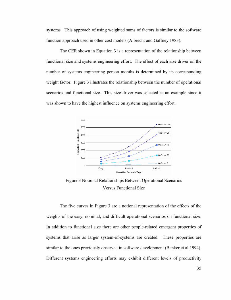
weight factor. Figure 3 illustrates the relationship between the number of operational
scenarios and functional size. This size driver was selected as an example since it
was shown to have the highest influence on systems engineering effort.
Figure 3 Notional Relationships Between Operational Scenarios
Versus Functional Size
The five curves in Figure 3 are a notional representation of the effects of the
weights of the easy, nominal, and difficult operational scenarios on functional size.
In addition to functional size there are other people-related emergent properties of
systems that arise as larger system-of-systems are created. These properties are
similar to the ones previously observed in software development (Banker et al 1994).
Different systems engineering efforts may exhibit different levels of productivity
36
which must be represented in COSYSMO. An exponential factor, E, is added to the
CER and is represented in Equation 4:
Equation 4 E
kddnneeNS wwwPM ⎟⎟⎠
⎞⎜⎜⎝
⎛Φ+Φ+Φ= ∑
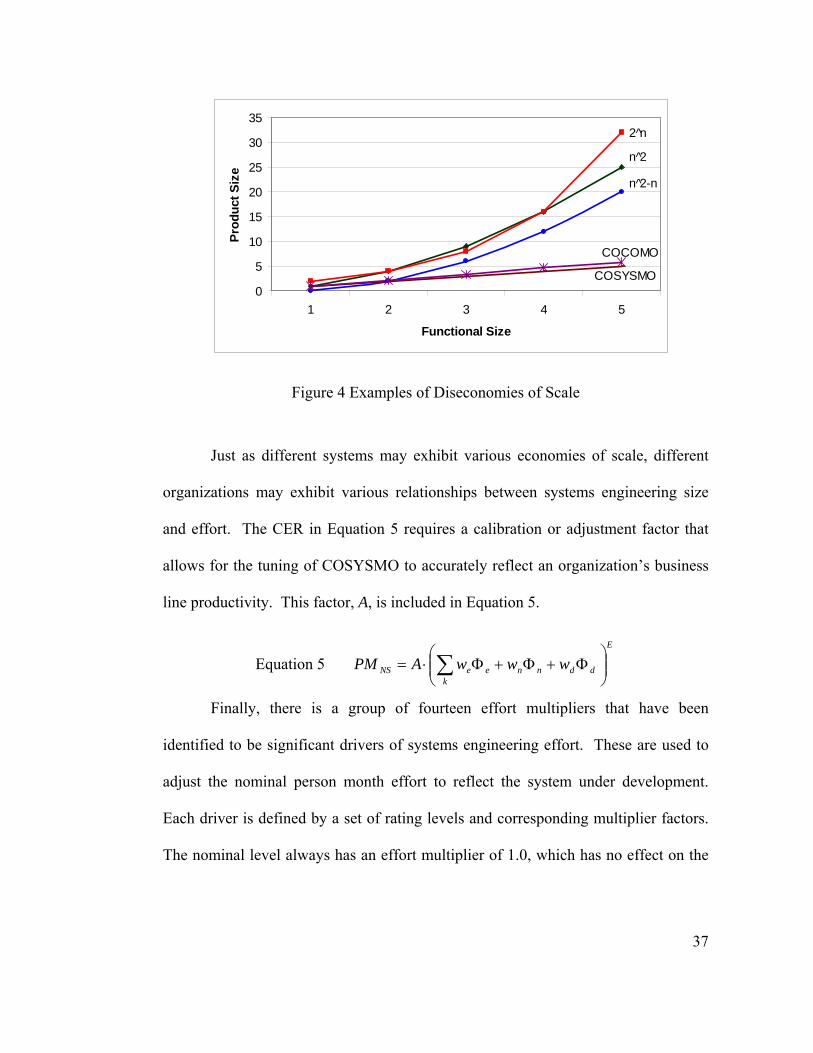
This factor relates to hypothesis #3. In the case of small projects the
exponent, E, could be equal to or less than 1.0. This would represent an economy of
scale which is generally very difficult to achieve in large people-intensive projects.
Most large projects would exhibit diseconomies of scale and as such would employ a
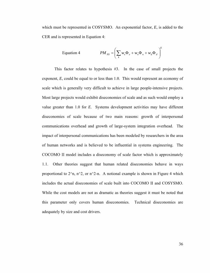
value greater than 1.0 for E. Systems development activities may have different
diseconomies of scale because of two main reasons: growth of interpersonal
communications overhead and growth of large-system integration overhead. The
impact of interpersonal communications has been modeled by researchers in the area
of human networks and is believed to be influential in systems engineering. The
COCOMO II model includes a diseconomy of scale factor which is approximately
1.1. Other theories suggest that human related diseconomies behave in ways
proportional to 2^n, n^2, or n^2-n. A notional example is shown in Figure 4 which
includes the actual diseconomies of scale built into COCOMO II and COSYSMO.
While the cost models are not as dramatic as theories suggest it must be noted that
this parameter only covers human diseconomies. Technical diseconomies are
adequately by size and cost drivers.
37
2 n̂
n 2̂
n 2̂-n
COSYSMO
COCOMO
0
5
10
15
20
25
30
35
1 2 3 4 5
Functional Size
Prod
uct S
ize
Figure 4 Examples of Diseconomies of Scale
Just as different systems may exhibit various economies of scale, different
organizations may exhibit various relationships between systems engineering size
and effort. The CER in Equation 5 requires a calibration or adjustment factor that
allows for the tuning of COSYSMO to accurately reflect an organization’s business
line productivity. This factor, A, is included in Equation 5.
Equation 5 E
kddnneeNS wwwAPM ⎟⎟⎠
⎞⎜⎜⎝
⎛Φ+Φ+Φ⋅= ∑
Finally, there is a group of fourteen effort multipliers that have been
identified to be significant drivers of systems engineering effort. These are used to
adjust the nominal person month effort to reflect the system under development.
Each driver is defined by a set of rating levels and corresponding multiplier factors.
The nominal level always has an effort multiplier of 1.0, which has no effect on the
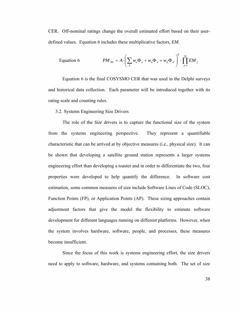
38
CER. Off-nominal ratings change the overall estimated effort based on their user-
defined values. Equation 6 includes these multiplicative factors, EM.
Equation 6 ∏∑=
⋅⎟⎟⎠
⎞⎜⎜⎝
⎛Φ+Φ+Φ⋅=
14
1jj
E
kddnneeNS EMwwwAPM
Equation 6 is the final COSYSMO CER that was used in the Delphi surveys
and historical data collection. Each parameter will be introduced together with its
rating scale and counting rules.
3.2. Systems Engineering Size Drivers
The role of the Size drivers is to capture the functional size of the system
from the systems engineering perspective. They represent a quantifiable
characteristic that can be arrived at by objective measures (i.e., physical size). It can
be shown that developing a satellite ground station represents a larger systems
engineering effort than developing a toaster and in order to differentiate the two, four
properties were developed to help quantify the difference. In software cost
estimation, some common measures of size include Software Lines of Code (SLOC),
Function Points (FP), or Application Points (AP). These sizing approaches contain
adjustment factors that give the model the flexibility to estimate software
development for different languages running on different platforms. However, when
the system involves hardware, software, people, and processes, these measures
become insufficient.
Since the focus of this work is systems engineering effort, the size drivers
need to apply to software, hardware, and systems containing both. The set of size
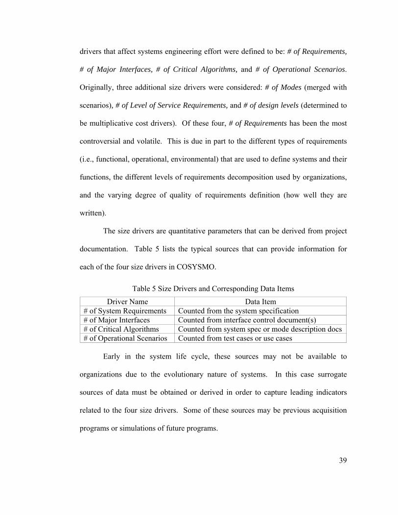
39
drivers that affect systems engineering effort were defined to be: # of Requirements,
# of Major Interfaces, # of Critical Algorithms, and # of Operational Scenarios.
Originally, three additional size drivers were considered: # of Modes (merged with
scenarios), # of Level of Service Requirements, and # of design levels (determined to
be multiplicative cost drivers). Of these four, # of Requirements has been the most
controversial and volatile. This is due in part to the different types of requirements
(i.e., functional, operational, environmental) that are used to define systems and their
functions, the different levels of requirements decomposition used by organizations,
and the varying degree of quality of requirements definition (how well they are
written).
The size drivers are quantitative parameters that can be derived from project
documentation. Table 5 lists the typical sources that can provide information for
each of the four size drivers in COSYSMO.
Table 5 Size Drivers and Corresponding Data Items
Driver Name Data Item # of System Requirements Counted from the system specification # of Major Interfaces Counted from interface control document(s) # of Critical Algorithms Counted from system spec or mode description docs # of Operational Scenarios Counted from test cases or use cases
Early in the system life cycle, these sources may not be available to
organizations due to the evolutionary nature of systems. In this case surrogate
sources of data must be obtained or derived in order to capture leading indicators
related to the four size drivers. Some of these sources may be previous acquisition
programs or simulations of future programs.
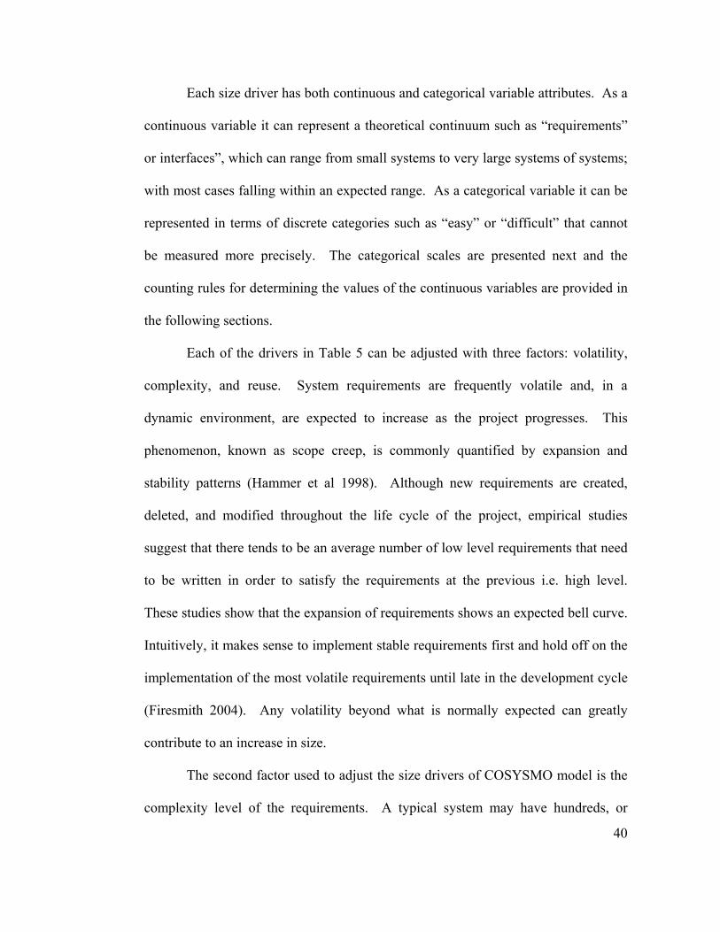
40
Each size driver has both continuous and categorical variable attributes. As a
continuous variable it can represent a theoretical continuum such as “requirements”
or interfaces”, which can range from small systems to very large systems of systems;
with most cases falling within an expected range. As a categorical variable it can be
represented in terms of discrete categories such as “easy” or “difficult” that cannot
be measured more precisely. The categorical scales are presented next and the
counting rules for determining the values of the continuous variables are provided in
the following sections.
Each of the drivers in Table 5 can be adjusted with three factors: volatility,
complexity, and reuse. System requirements are frequently volatile and, in a
dynamic environment, are expected to increase as the project progresses. This
phenomenon, known as scope creep, is commonly quantified by expansion and
stability patterns (Hammer et al 1998). Although new requirements are created,
deleted, and modified throughout the life cycle of the project, empirical studies
suggest that there tends to be an average number of low level requirements that need
to be written in order to satisfy the requirements at the previous i.e. high level.
These studies show that the expansion of requirements shows an expected bell curve.
Intuitively, it makes sense to implement stable requirements first and hold off on the
implementation of the most volatile requirements until late in the development cycle
(Firesmith 2004). Any volatility beyond what is normally expected can greatly
contribute to an increase in size.
The second factor used to adjust the size drivers of COSYSMO model is the
complexity level of the requirements. A typical system may have hundreds, or
41
potentially thousands, of requirements that are decomposed further into requirements
pertaining to the next subsystem. Naturally, not all requirements have the same level
of complexity. Some may be more complex than others based on how well they are
specified, how easily they are traceable to their source, and how much they overlap
with other requirements. It has been determined that a simple sum of the total
number of requirements is not a reliable indicator of functional size. Instead, the
sum of the requirements requires a complexity weight to reflect the corresponding
complexity of each requirement. Logically, the more complex a requirement the
greater the weight that is assigned to it. It is up to the individual organization to
make an assessment of the complexity of the size drivers associated with their
systems. Guidance on how to accomplish this for each size driver is provided in the
next sections.
Reuse is the third important factor used to adjust the number of requirements.
As reuse facilitates the usage of certain components in the system it tends to bring
down the efforts involved in the system development. The sum of requirements is
adjusted downwards when there are a significant number of reused requirements.
This is meant to capture an organization’s familiarity with the development,
management, and testing of requirements. However, reused requirements are not
free from systems engineering effort. There are three components of reuse each of
which has a cost: redesign, reimplementation, and retest. Redesign is necessary
when the existing functionality may not be exactly suited to the new task. When this
is so, the application to be reused will likely require some rework to support new
functions, and it may require reverse engineering to understand its current operation.
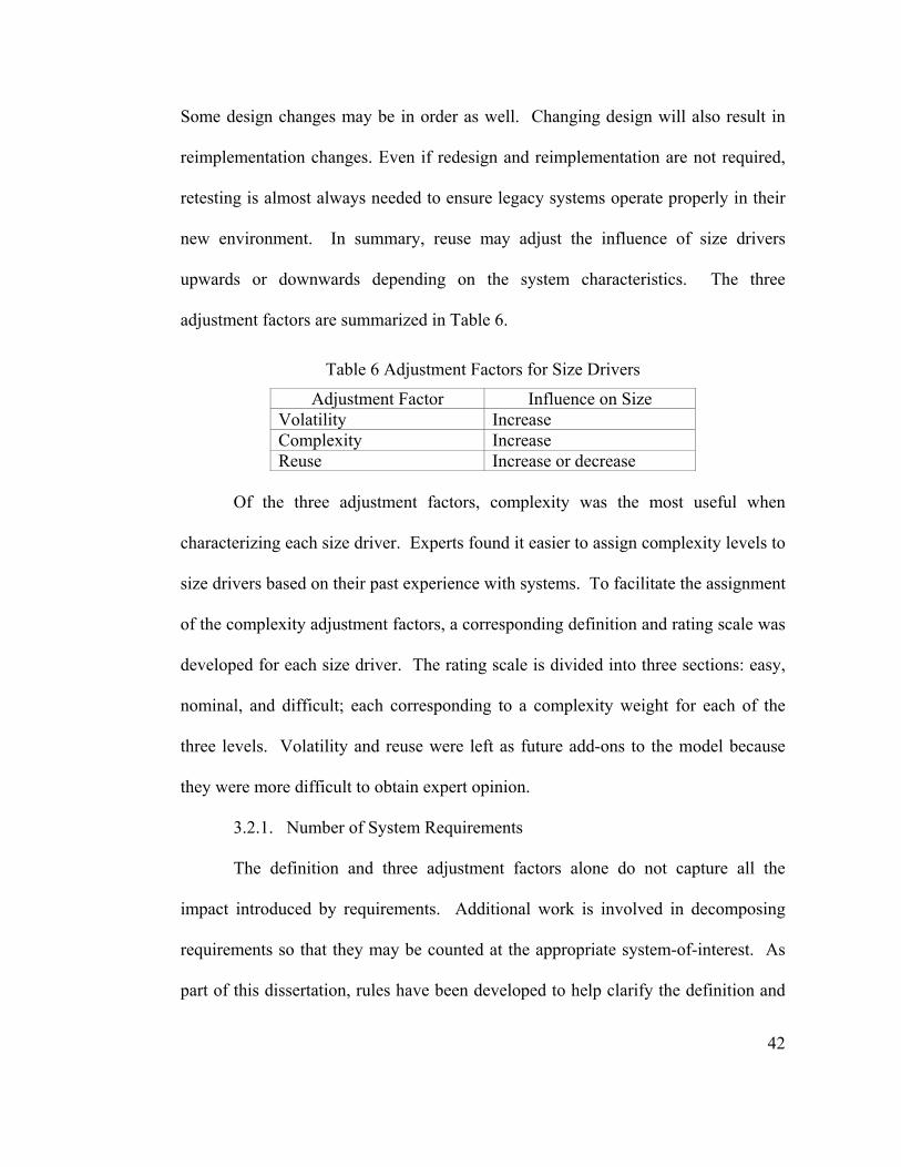
42
Some design changes may be in order as well. Changing design will also result in
reimplementation changes. Even if redesign and reimplementation are not required,
retesting is almost always needed to ensure legacy systems operate properly in their
new environment. In summary, reuse may adjust the influence of size drivers
upwards or downwards depending on the system characteristics. The three
adjustment factors are summarized in Table 6.
Table 6 Adjustment Factors for Size Drivers
Adjustment Factor Influence on Size Volatility Increase Complexity Increase Reuse Increase or decrease
Of the three adjustment factors, complexity was the most useful when
characterizing each size driver. Experts found it easier to assign complexity levels to
size drivers based on their past experience with systems. To facilitate the assignment
of the complexity adjustment factors, a corresponding definition and rating scale was
developed for each size driver. The rating scale is divided into three sections: easy,
nominal, and difficult; each corresponding to a complexity weight for each of the
three levels. Volatility and reuse were left as future add-ons to the model because
they were more difficult to obtain expert opinion.
3.2.1. Number of System Requirements
The definition and three adjustment factors alone do not capture all the
impact introduced by requirements. Additional work is involved in decomposing
requirements so that they may be counted at the appropriate system-of-interest. As
part of this dissertation, rules have been developed to help clarify the definition and
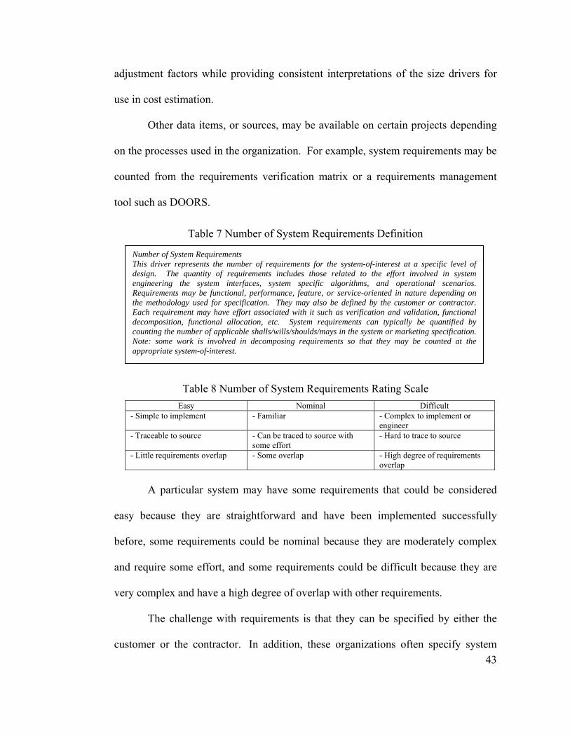
43
adjustment factors while providing consistent interpretations of the size drivers for
use in cost estimation.
Other data items, or sources, may be available on certain projects depending
on the processes used in the organization. For example, system requirements may be
counted from the requirements verification matrix or a requirements management
tool such as DOORS.
Table 7 Number of System Requirements Definition
Table 8 Number of System Requirements Rating Scale Easy Nominal Difficult
- Simple to implement - Familiar - Complex to implement or engineer
- Traceable to source - Can be traced to source with some effort
- Hard to trace to source
- Little requirements overlap - Some overlap - High degree of requirements overlap
A particular system may have some requirements that could be considered
easy because they are straightforward and have been implemented successfully
before, some requirements could be nominal because they are moderately complex
and require some effort, and some requirements could be difficult because they are
very complex and have a high degree of overlap with other requirements.
The challenge with requirements is that they can be specified by either the
customer or the contractor. In addition, these organizations often specify system
Number of System Requirements This driver represents the number of requirements for the system-of-interest at a specific level of design. The quantity of requirements includes those related to the effort involved in system engineering the system interfaces, system specific algorithms, and operational scenarios. Requirements may be functional, performance, feature, or service-oriented in nature depending on the methodology used for specification. They may also be defined by the customer or contractor. Each requirement may have effort associated with it such as verification and validation, functional decomposition, functional allocation, etc. System requirements can typically be quantified by counting the number of applicable shalls/wills/shoulds/mays in the system or marketing specification. Note: some work is involved in decomposing requirements so that they may be counted at the appropriate system-of-interest.
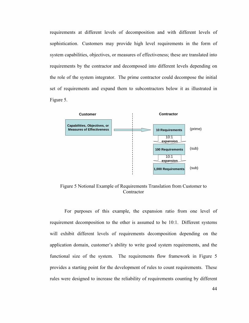
44
requirements at different levels of decomposition and with different levels of
sophistication. Customers may provide high level requirements in the form of
system capabilities, objectives, or measures of effectiveness; these are translated into
requirements by the contractor and decomposed into different levels depending on
the role of the system integrator. The prime contractor could decompose the initial
set of requirements and expand them to subcontractors below it as illustrated in
Figure 5.
Customer Contractor
Capabilities, Objectives, or Measures of Effectiveness 10 Requirements (prime)
100 Requirements (sub)
10:1 expansion
1,000 Requirements (sub)
10:1 expansion
Figure 5 Notional Example of Requirements Translation from Customer to Contractor
For purposes of this example, the expansion ratio from one level of
requirement decomposition to the other is assumed to be 10:1. Different systems
will exhibit different levels of requirements decomposition depending on the
application domain, customer’s ability to write good system requirements, and the
functional size of the system. The requirements flow framework in Figure 5
provides a starting point for the development of rules to count requirements. These
rules were designed to increase the reliability of requirements counting by different
45
organizations on different systems regardless of their application domain. The five
rules are as follows:
1. Determine the system of interest. For an airplane, the system of interest
may be the avionics subsystem or the entire airplane depending on the
perspective of the organization interested in estimating systems
engineering. This key decision needs to be made early on to determine the
scope of the COSYSMO estimate and identify the requirements that are
applicable for the chosen system.
2. Decompose system objectives, capabilities, or measures of effectiveness
into requirements that can be tested, verified, or designed. The
decomposition of requirements must be performed by the organization using
COSYSMO. The level of decomposition of interest for COSYSMO is the
level in which the system will be designed and tested; which is equivalent to
the TYPE A, System/Segment Specification (MIL-STD 490-A 1985).
3. Provide a graphical or narrative representation of the system of interest
and how it relates to the rest of the system. This step focuses on the
hierarchical relationship between the system elements. This information can
help describe the size of the system and its levels of design. It serves as a
sanity check for the previous two steps.
4. Count the number of requirements in the system/marketing specification
or the verification test matrix for the level of design in which systems
engineering is taking place in the desired system of interest. The focus of
the counted requirements needs to be for systems engineering. Lower level
46
requirements may not be applicable if they have no effect on systems
engineering. Requirements may be counted from the Requirements
Verification Trace Matrix (RVTM) that is used for testing system
requirements. The same rules apply as before: all counted requirements must
be at the same design or bid level and lower level requirements must be
disregarded if they do not influence systems engineering effort.
5. Determine the volatility, complexity, and reuse of requirements. Once
the quantity of requirements has been determined, the three adjustment
factors can be applied. Currently three complexity factors have been
determined: easy, nominal, and difficult. These weights for these factors
were determined using expert opinion through the use of a Delphi survey
(Valerdi et al 2003). The volatility and reuse factors are optional and depend
on the version of COSYSMO implementation being used.
The objective of the five steps is to lead users down a consistent path of
similar logic when determining the number of system requirements for the purposes
of estimating systems engineering effort in COSYSMO. It has been found that the
level of decomposition described in step #2 may be the most volatile step as
indicated by the data collected thus far. To alleviate this, a framework of software
use case decomposition was adopted (Cockburn 2001). The basic premise behind
the framework is that different levels exist for specific system functions. Choosing
the appropriate level can provide a focused basis for describing the customer and
developer needs. A metaphor is used to describe four levels: sky level, kite level, sea
level, and underwater level. The development of COSYSMO can be used to further
47
illustrate the sea level metaphor. The summary level, or sky level, represents the
highest level that describes either a strategic or system scope.
For example, a sky level goal for COSYSMO is to “build a systems
engineering cost model.” The stakeholders of the model stated this as their basic
need that in turn drives a collection of user level goals. A kite level goal provides
more detailed information as to “how” the sky level goal will be satisfied.
Continuing the example, it includes the standards that will drive the definition of
systems engineering and system life cycle phases. The sea level goals represent a
user level task that is the target level for counting requirements in COSYSMO. It
involves utilizing size and cost drivers, definitions, and counting rules that will
enable the accurate estimation of systems engineering effort, also providing more
information on how the higher goals at the kite level will be satisfied. The sea level
is also important because it describes the environment in which the model developers
interact with the users and stakeholders. A step below is the underwater level which
is of more concern to the developer. In this example, it involves the selection of
implementation and analysis tools required to meet the user goals. The examples are
mapped to Cockburn’s hierarchy in Figure 6.
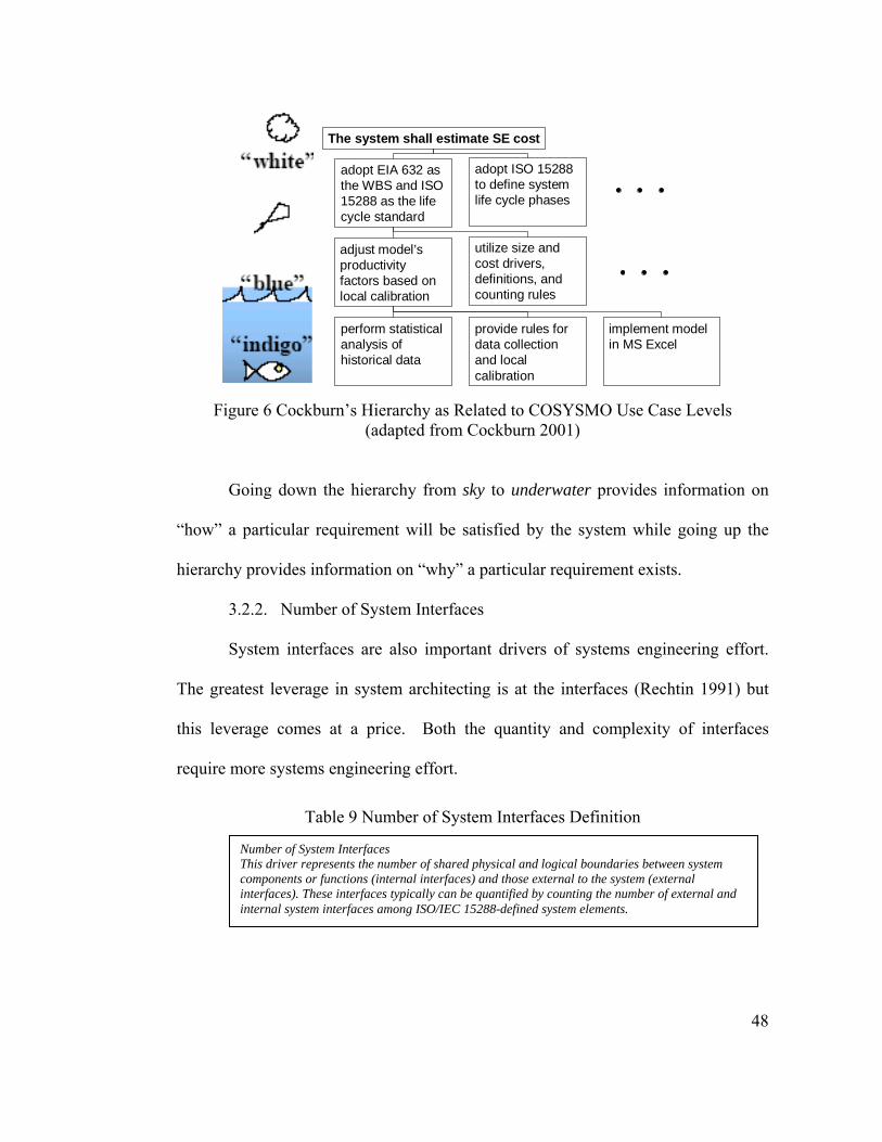
48
perform statistical analysis of historical data
The system shall estimate SE cost
adopt EIA 632 as the WBS and ISO 15288 as the life cycle standard
adjust model’s productivity factors based on local calibration
utilize size and cost drivers, definitions, and counting rules
provide rules for data collection and local calibration
implement model in MS Excel
adopt ISO 15288 to define system life cycle phases
Figure 6 Cockburn’s Hierarchy as Related to COSYSMO Use Case Levels
(adapted from Cockburn 2001)
Going down the hierarchy from sky to underwater provides information on
“how” a particular requirement will be satisfied by the system while going up the
hierarchy provides information on “why” a particular requirement exists.
3.2.2. Number of System Interfaces
System interfaces are also important drivers of systems engineering effort.
The greatest leverage in system architecting is at the interfaces (Rechtin 1991) but
this leverage comes at a price. Both the quantity and complexity of interfaces
require more systems engineering effort.
Table 9 Number of System Interfaces Definition
Number of System Interfaces This driver represents the number of shared physical and logical boundaries between system components or functions (internal interfaces) and those external to the system (external interfaces). These interfaces typically can be quantified by counting the number of external and internal system interfaces among ISO/IEC 15288-defined system elements.
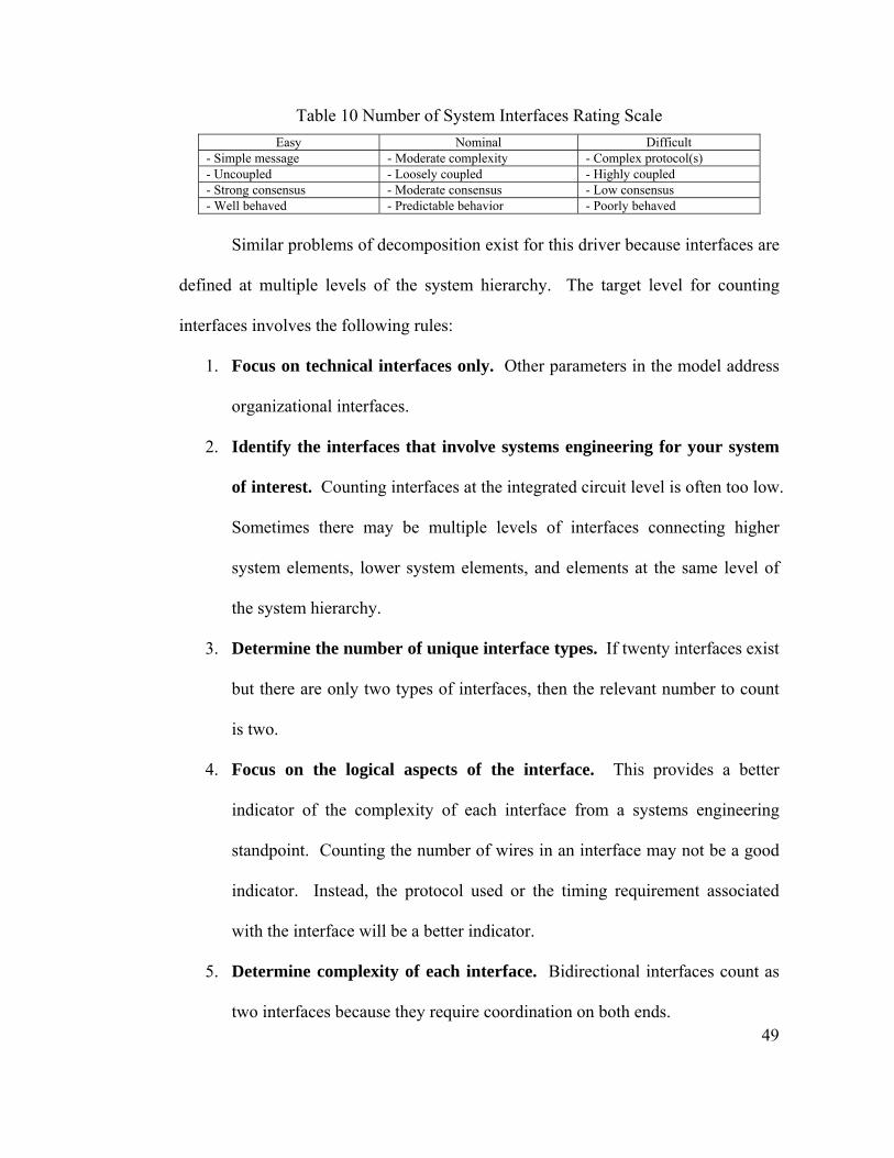
49
Table 10 Number of System Interfaces Rating Scale Easy Nominal Difficult
- Simple message - Moderate complexity - Complex protocol(s) - Uncoupled - Loosely coupled - Highly coupled - Strong consensus - Moderate consensus - Low consensus - Well behaved - Predictable behavior - Poorly behaved
Similar problems of decomposition exist for this driver because interfaces are
defined at multiple levels of the system hierarchy. The target level for counting
interfaces involves the following rules:
1. Focus on technical interfaces only. Other parameters in the model address
organizational interfaces.
2. Identify the interfaces that involve systems engineering for your system
of interest. Counting interfaces at the integrated circuit level is often too low.
Sometimes there may be multiple levels of interfaces connecting higher
system elements, lower system elements, and elements at the same level of
the system hierarchy.
3. Determine the number of unique interface types. If twenty interfaces exist
but there are only two types of interfaces, then the relevant number to count
is two.
4. Focus on the logical aspects of the interface. This provides a better
indicator of the complexity of each interface from a systems engineering
standpoint. Counting the number of wires in an interface may not be a good
indicator. Instead, the protocol used or the timing requirement associated
with the interface will be a better indicator.
5. Determine complexity of each interface. Bidirectional interfaces count as
two interfaces because they require coordination on both ends.
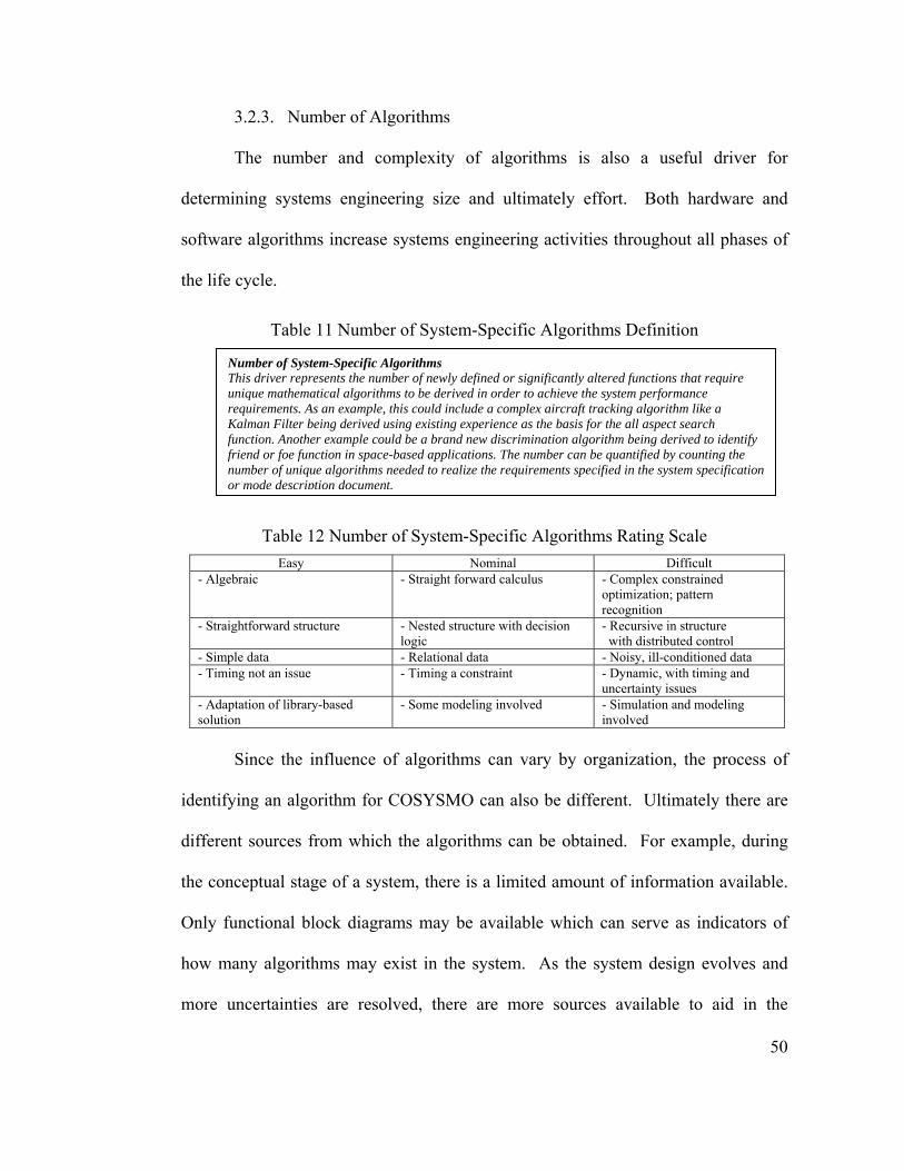
50
3.2.3. Number of Algorithms
The number and complexity of algorithms is also a useful driver for
determining systems engineering size and ultimately effort. Both hardware and
software algorithms increase systems engineering activities throughout all phases of
the life cycle.
Table 11 Number of System-Specific Algorithms Definition
Table 12 Number of System-Specific Algorithms Rating Scale Easy Nominal Difficult
- Algebraic - Straight forward calculus - Complex constrained optimization; pattern recognition
- Straightforward structure - Nested structure with decision logic
- Recursive in structure with distributed control
- Simple data - Relational data - Noisy, ill-conditioned data - Timing not an issue - Timing a constraint - Dynamic, with timing and
uncertainty issues - Adaptation of library-based solution
- Some modeling involved - Simulation and modeling involved
Since the influence of algorithms can vary by organization, the process of
identifying an algorithm for COSYSMO can also be different. Ultimately there are
different sources from which the algorithms can be obtained. For example, during
the conceptual stage of a system, there is a limited amount of information available.
Only functional block diagrams may be available which can serve as indicators of
how many algorithms may exist in the system. As the system design evolves and
more uncertainties are resolved, there are more sources available to aid in the
Number of System-Specific Algorithms This driver represents the number of newly defined or significantly altered functions that require unique mathematical algorithms to be derived in order to achieve the system performance requirements. As an example, this could include a complex aircraft tracking algorithm like a Kalman Filter being derived using existing experience as the basis for the all aspect search function. Another example could be a brand new discrimination algorithm being derived to identify friend or foe function in space-based applications. The number can be quantified by counting the number of unique algorithms needed to realize the requirements specified in the system specification or mode description document.
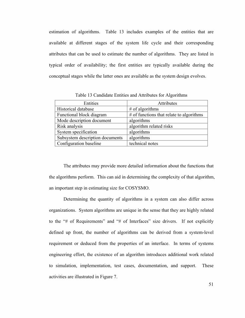
51
estimation of algorithms. Table 13 includes examples of the entities that are
available at different stages of the system life cycle and their corresponding
attributes that can be used to estimate the number of algorithms. They are listed in
typical order of availability; the first entities are typically available during the
conceptual stages while the latter ones are available as the system design evolves.
Table 13 Candidate Entities and Attributes for Algorithms
Entities Attributes Historical database # of algorithms Functional block diagram # of functions that relate to algorithms Mode description document algorithms Risk analysis algorithm related risks System specification algorithms Subsystem description documents algorithms Configuration baseline technical notes
The attributes may provide more detailed information about the functions that
the algorithms perform. This can aid in determining the complexity of that algorithm,
an important step in estimating size for COSYSMO.
Determining the quantity of algorithms in a system can also differ across
organizations. System algorithms are unique in the sense that they are highly related
to the “# of Requirements” and “# of Interfaces” size drivers. If not explicitly
defined up front, the number of algorithms can be derived from a system-level
requirement or deduced from the properties of an interface. In terms of systems
engineering effort, the existence of an algorithm introduces additional work related
to simulation, implementation, test cases, documentation, and support. These
activities are illustrated in Figure 7.
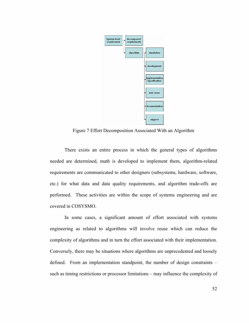
52
Figure 7 Effort Decomposition Associated With an Algorithm
There exists an entire process in which the general types of algorithms
needed are determined, math is developed to implement them, algorithm-related
requirements are communicated to other designers (subsystems, hardware, software,
etc.) for what data and data quality requirements, and algorithm trade-offs are
performed. These activities are within the scope of systems engineering and are
covered in COSYSMO.
In some cases, a significant amount of effort associated with systems
engineering as related to algorithms will involve reuse which can reduce the
complexity of algorithms and in turn the effort associated with their implementation.
Conversely, there may be situations where algorithms are unprecedented and loosely
defined. From an implementation standpoint, the number of design constraints –
such as timing restrictions or processor limitations – may influence the complexity of
53
software algorithms when compared to hardware algorithms. In either case, both
types of algorithms should be counted and assigned a level of complexity for input
into COSYSMO.
To demonstrate the process of identifying and counting an algorithm an
example is provided from the field of signal compression. For purposes of this
example it is assumed that a system specification has been developed. From this
specification, the following system level requirement is obtained: All images
captured by the sensor shall be compressed in compliance with MPEG-4 coding
standard. This requirement triggers several possible solutions that meet the required
standard. A developer may decide to implement the requirement with a well-known
algorithm used for compressing visual images: MPEG-4 Visual Texture Coding
(VTC). As illustrated in Figure 7 this algorithm generates products associated with it
which lead to increased systems engineering effort that is estimated by COSYSMO.
Other effort generated by the implementation specification, such as software
engineering, is not estimated by COSYSMO. Models such as COCOMO II should
be used to estimate the software development effort. For purposes of COSYSMO,
the MPEG-4 VTC algorithm counts as one distinct algorithm even if it is used
multiple times in the same system. Since this is a well known algorithm with
predictable behavior it qualifies as an “easy” algorithm.
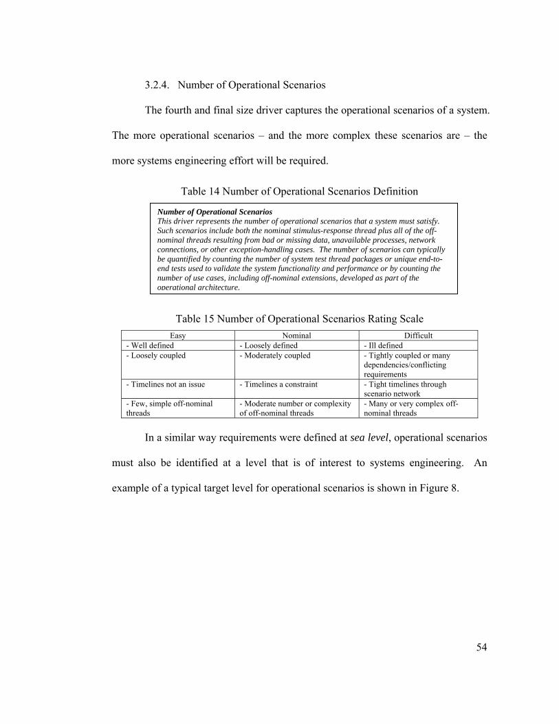
54
3.2.4. Number of Operational Scenarios
The fourth and final size driver captures the operational scenarios of a system.
The more operational scenarios – and the more complex these scenarios are – the
more systems engineering effort will be required.
Table 14 Number of Operational Scenarios Definition
Table 15 Number of Operational Scenarios Rating Scale Easy Nominal Difficult
- Well defined - Loosely defined - Ill defined - Loosely coupled - Moderately coupled - Tightly coupled or many
dependencies/conflicting requirements
- Timelines not an issue - Timelines a constraint - Tight timelines through scenario network
- Few, simple off-nominal threads
- Moderate number or complexity of off-nominal threads
- Many or very complex off-nominal threads
In a similar way requirements were defined at sea level, operational scenarios
must also be identified at a level that is of interest to systems engineering. An
example of a typical target level for operational scenarios is shown in Figure 8.
Number of Operational Scenarios This driver represents the number of operational scenarios that a system must satisfy. Such scenarios include both the nominal stimulus-response thread plus all of the off-nominal threads resulting from bad or missing data, unavailable processes, network connections, or other exception-handling cases. The number of scenarios can typically be quantified by counting the number of system test thread packages or unique end-to-end tests used to validate the system functionality and performance or by counting the number of use cases, including off-nominal extensions, developed as part of the operational architecture.
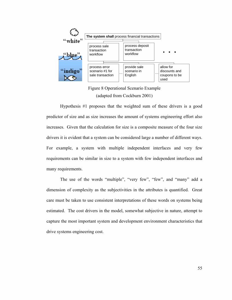
55
process error scenario #1 for sale transaction
The system shall process financial transactions
process sale transaction workflow
process deposit transaction workflow
provide sale scenario in English
allow for discounts and coupons to be used
… …
Figure 8 Operational Scenario Example
(adapted from Cockburn 2001)
Hypothesis #1 proposes that the weighted sum of these drivers is a good
predictor of size and as size increases the amount of systems engineering effort also
increases. Given that the calculation for size is a composite measure of the four size
drivers it is evident that a system can be considered large a number of different ways.
For example, a system with multiple independent interfaces and very few
requirements can be similar in size to a system with few independent interfaces and
many requirements.
The use of the words “multiple”, “very few”, “few”, and “many” add a
dimension of complexity as the subjectivities in the attributes is quantified. Great
care must be taken to use consistent interpretations of these words on systems being
estimated. The cost drivers in the model, somewhat subjective in nature, attempt to
capture the most important system and development environment characteristics that
drive systems engineering cost.
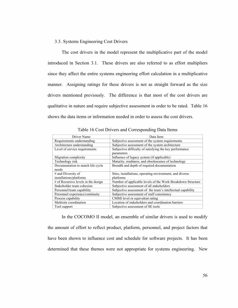
56
3.3. Systems Engineering Cost Drivers
The cost drivers in the model represent the multiplicative part of the model
introduced in Section 3.1. These drivers are also referred to as effort multipliers
since they affect the entire systems engineering effort calculation in a multiplicative
manner. Assigning ratings for these drivers is not as straight forward as the size
drivers mentioned previously. The difference is that most of the cost drivers are
qualitative in nature and require subjective assessment in order to be rated. Table 16
shows the data items or information needed in order to assess the cost drivers.
Table 16 Cost Drivers and Corresponding Data Items Driver Name Data Item
Requirements understanding Subjective assessment of the system requirements Architecture understanding Subjective assessment of the system architecture Level of service requirements Subjective difficulty of satisfying the key performance
parameters Migration complexity Influence of legacy system (if applicable) Technology risk Maturity, readiness, and obsolescence of technology Documentation to match life cycle needs
Breadth and depth of required documentation
# and Diversity of installations/platforms
Sites, installations, operating environment, and diverse platforms
# of Recursive levels in the design Number of applicable levels of the Work Breakdown Structure Stakeholder team cohesion Subjective assessment of all stakeholders Personnel/team capability Subjective assessment of the team’s intellectual capability Personnel experience/continuity Subjective assessment of staff consistency Process capability CMMI level or equivalent rating Multisite coordination Location of stakeholders and coordination barriers Tool support Subjective assessment of SE tools
In the COCOMO II model, an ensemble of similar drivers is used to modify
the amount of effort to reflect product, platform, personnel, and project factors that
have been shown to influence cost and schedule for software projects. It has been
determined that these themes were not appropriate for systems engineering. New
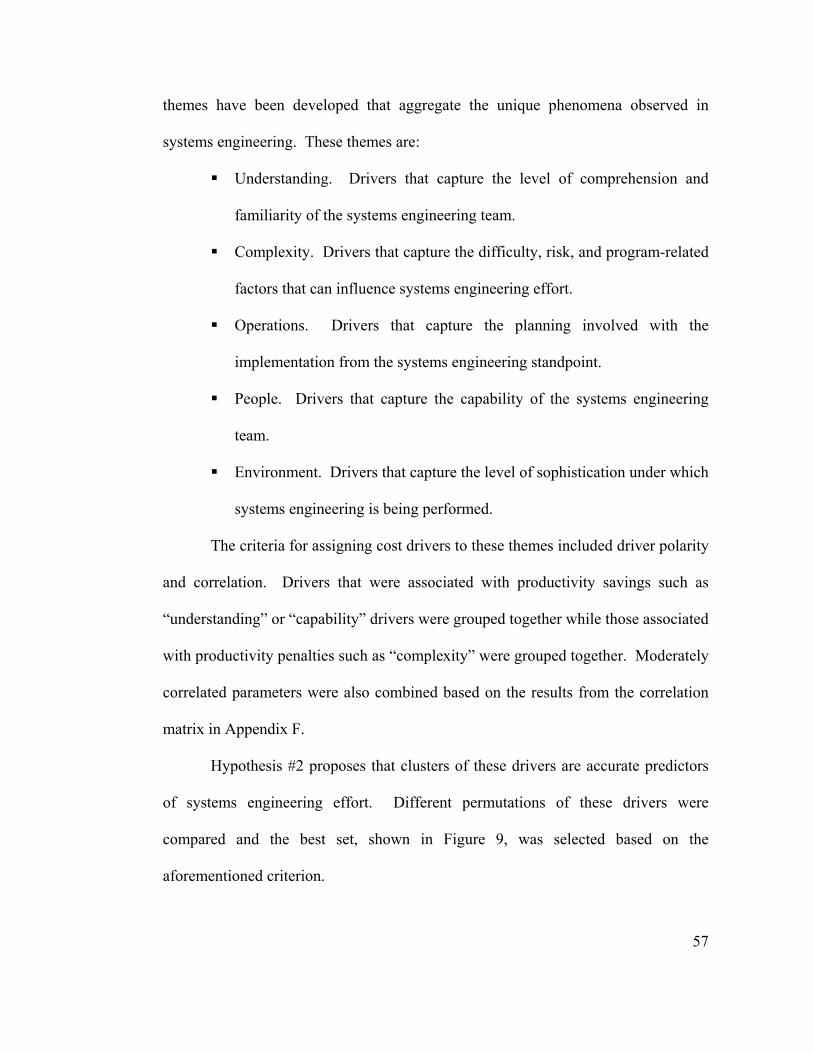
57
themes have been developed that aggregate the unique phenomena observed in
systems engineering. These themes are:
Understanding. Drivers that capture the level of comprehension and
familiarity of the systems engineering team.
Complexity. Drivers that capture the difficulty, risk, and program-related
factors that can influence systems engineering effort.
Operations. Drivers that capture the planning involved with the
implementation from the systems engineering standpoint.
People. Drivers that capture the capability of the systems engineering
team.
Environment. Drivers that capture the level of sophistication under which
systems engineering is being performed.
The criteria for assigning cost drivers to these themes included driver polarity
and correlation. Drivers that were associated with productivity savings such as
“understanding” or “capability” drivers were grouped together while those associated
with productivity penalties such as “complexity” were grouped together. Moderately
correlated parameters were also combined based on the results from the correlation
matrix in Appendix F.
Hypothesis #2 proposes that clusters of these drivers are accurate predictors
of systems engineering effort. Different permutations of these drivers were
compared and the best set, shown in Figure 9, was selected based on the
aforementioned criterion.
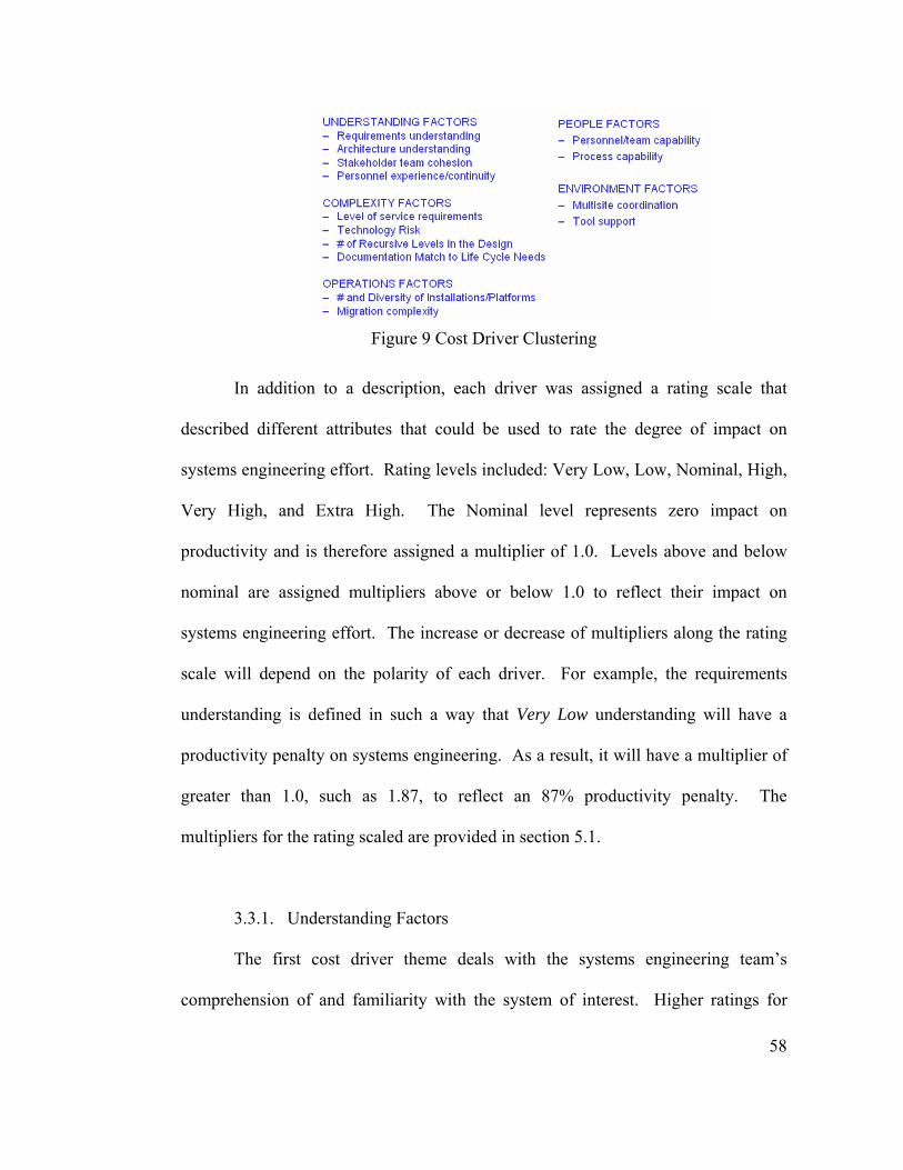
58
Figure 9 Cost Driver Clustering
In addition to a description, each driver was assigned a rating scale that
described different attributes that could be used to rate the degree of impact on
systems engineering effort. Rating levels included: Very Low, Low, Nominal, High,
Very High, and Extra High. The Nominal level represents zero impact on
productivity and is therefore assigned a multiplier of 1.0. Levels above and below
nominal are assigned multipliers above or below 1.0 to reflect their impact on
systems engineering effort. The increase or decrease of multipliers along the rating
scale will depend on the polarity of each driver. For example, the requirements
understanding is defined in such a way that Very Low understanding will have a
productivity penalty on systems engineering. As a result, it will have a multiplier of
greater than 1.0, such as 1.87, to reflect an 87% productivity penalty. The
multipliers for the rating scaled are provided in section 5.1.
3.3.1. Understanding Factors
The first cost driver theme deals with the systems engineering team’s
comprehension of and familiarity with the system of interest. Higher ratings for
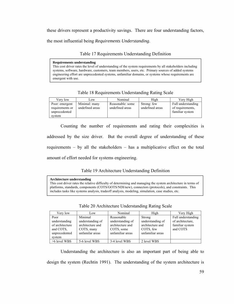
59
these drivers represent a productivity savings. There are four understanding factors,
the most influential being Requirements Understanding.
Table 17 Requirements Understanding Definition
Table 18 Requirements Understanding Rating Scale Very low Low Nominal High Very High
Poor: emergent requirements or unprecedented system
Minimal: many undefined areas
Reasonable: some undefined areas
Strong: few undefined areas
Full understanding of requirements, familiar system
Counting the number of requirements and rating their complexities is
addressed by the size driver. But the overall degree of understanding of these
requirements – by all the stakeholders – has a multiplicative effect on the total
amount of effort needed for systems engineering.
Table 19 Architecture Understanding Definition
Table 20 Architecture Understanding Rating Scale Very low Low Nominal High Very High
Poor understanding of architecture and COTS, unprecedented system
Minimal understanding of architecture and COTS, many unfamilar areas
Reasonable understanding of architecture and COTS, some unfamiliar areas
Strong understanding of architecture and COTS, few unfamiliar areas
Full understanding of architecture, familiar system and COTS
>6 level WBS 5-6 level WBS 3-4 level WBS 2 level WBS Understanding the architecture is also an important part of being able to
design the system (Rechtin 1991). The understanding of the system architecture is
Architecture understanding This cost driver rates the relative difficulty of determining and managing the system architecture in terms of platforms, standards, components (COTS/GOTS/NDI/new), connectors (protocols), and constraints. This includes tasks like systems analysis, tradeoff analysis, modeling, simulation, case studies, etc.
Requirements understanding This cost driver rates the level of understanding of the system requirements by all stakeholders including systems, software, hardware, customers, team members, users, etc. Primary sources of added systems engineering effort are unprecedented systems, unfamiliar domains, or systems whose requirements are emergent with use.
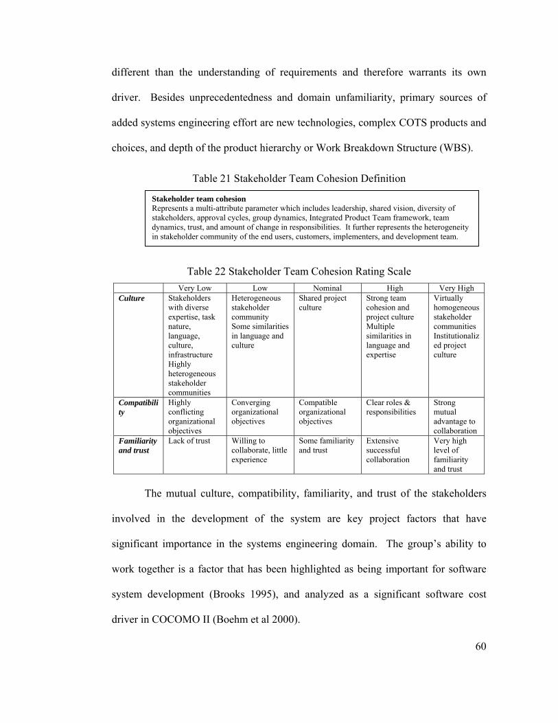
60
different than the understanding of requirements and therefore warrants its own
driver. Besides unprecedentedness and domain unfamiliarity, primary sources of
added systems engineering effort are new technologies, complex COTS products and
choices, and depth of the product hierarchy or Work Breakdown Structure (WBS).
Table 21 Stakeholder Team Cohesion Definition
Table 22 Stakeholder Team Cohesion Rating Scale Very Low Low Nominal High Very High Culture Stakeholders
with diverse expertise, task nature, language, culture, infrastructure Highly heterogeneous stakeholder communities
Heterogeneous stakeholder community Some similarities in language and culture
Shared project culture
Strong team cohesion and project culture Multiple similarities in language and expertise
Virtually homogeneous stakeholder communities Institutionalized project culture
Compatibility
Highly conflicting organizational objectives
Converging organizational objectives
Compatible organizational objectives
Clear roles & responsibilities
Strong mutual advantage to collaboration
Familiarity and trust
Lack of trust Willing to collaborate, little experience
Some familiarity and trust
Extensive successful collaboration
Very high level of familiarity and trust
The mutual culture, compatibility, familiarity, and trust of the stakeholders
involved in the development of the system are key project factors that have
significant importance in the systems engineering domain. The group’s ability to
work together is a factor that has been highlighted as being important for software
system development (Brooks 1995), and analyzed as a significant software cost
driver in COCOMO II (Boehm et al 2000).
Stakeholder team cohesion Represents a multi-attribute parameter which includes leadership, shared vision, diversity of stakeholders, approval cycles, group dynamics, Integrated Product Team framework, team dynamics, trust, and amount of change in responsibilities. It further represents the heterogeneity in stakeholder community of the end users, customers, implementers, and development team.
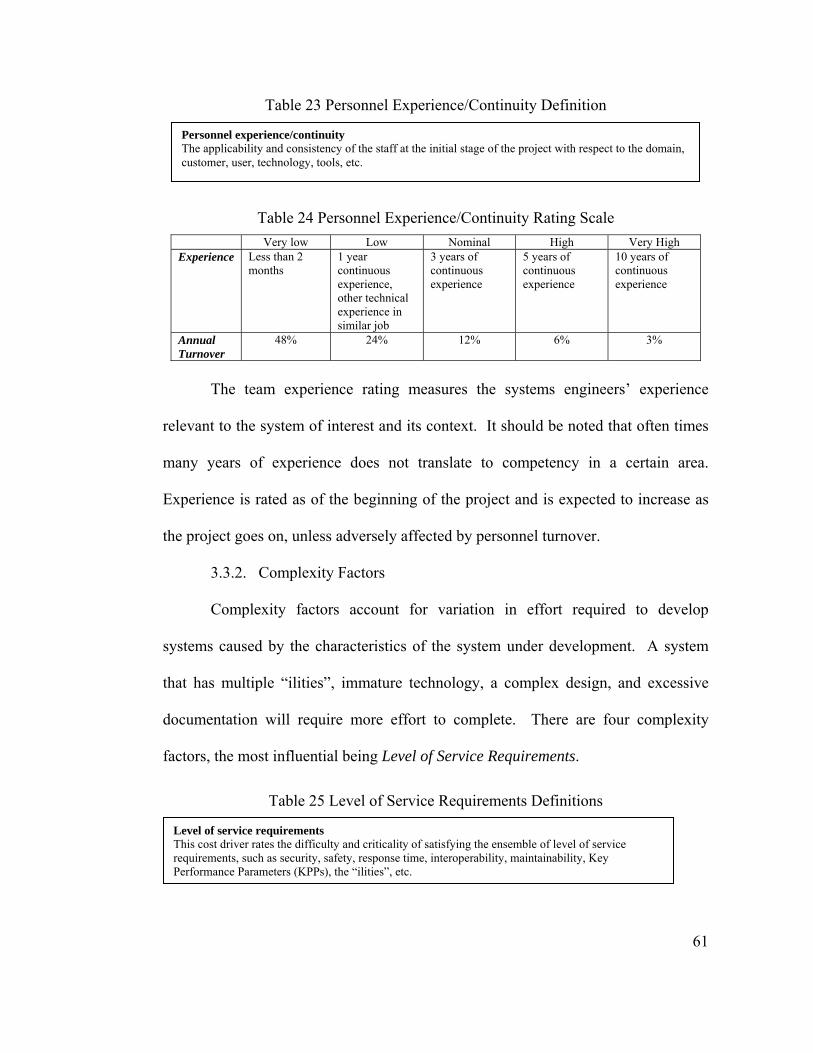
61
Table 23 Personnel Experience/Continuity Definition
Table 24 Personnel Experience/Continuity Rating Scale Very low Low Nominal High Very High Experience Less than 2
months 1 year continuous experience, other technical experience in similar job
3 years of continuous experience
5 years of continuous experience
10 years of continuous experience
Annual Turnover
48% 24% 12% 6% 3%
The team experience rating measures the systems engineers’ experience
relevant to the system of interest and its context. It should be noted that often times
many years of experience does not translate to competency in a certain area.
Experience is rated as of the beginning of the project and is expected to increase as
the project goes on, unless adversely affected by personnel turnover.
3.3.2. Complexity Factors
Complexity factors account for variation in effort required to develop
systems caused by the characteristics of the system under development. A system
that has multiple “ilities”, immature technology, a complex design, and excessive
documentation will require more effort to complete. There are four complexity
factors, the most influential being Level of Service Requirements.
Table 25 Level of Service Requirements Definitions
Level of service requirements This cost driver rates the difficulty and criticality of satisfying the ensemble of level of service requirements, such as security, safety, response time, interoperability, maintainability, Key Performance Parameters (KPPs), the “ilities”, etc.
Personnel experience/continuity The applicability and consistency of the staff at the initial stage of the project with respect to the domain, customer, user, technology, tools, etc.
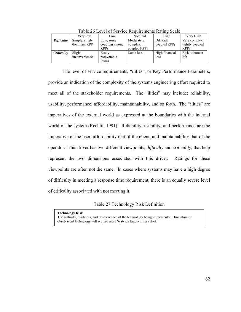
62
Table 26 Level of Service Requirements Rating Scale Very low Low Nominal High Very High
Difficulty Simple; single dominant KPP
Low, some coupling among KPPs
Moderately complex, coupled KPPs
Difficult, coupled KPPs
Very complex, tightly coupled KPPs
Criticality Slight inconvenience
Easily recoverable losses
Some loss High financial loss
Risk to human life
The level of service requirements, “ilities”, or Key Performance Parameters,
provide an indication of the complexity of the systems engineering effort required to
meet all of the stakeholder requirements. The “ilities” may include: reliability,
usability, performance, affordability, maintainability, and so forth. The “ilities” are
imperatives of the external world as expressed at the boundaries with the internal
world of the system (Rechtin 1991). Reliability, usability, and performance are the
imperative of the user, affordability that of the client, and maintainability that of the
operator. This driver has two different viewpoints, difficulty and criticality, that help
represent the two dimensions associated with this driver. Ratings for these
viewpoints are often not the same. In cases where systems may have a high degree
of difficulty in meeting a response time requirement, there is an equally severe level
of criticality associated with not meeting it.
Table 27 Technology Risk Definition
Technology Risk The maturity, readiness, and obsolescence of the technology being implemented. Immature or obsolescent technology will require more Systems Engineering effort.
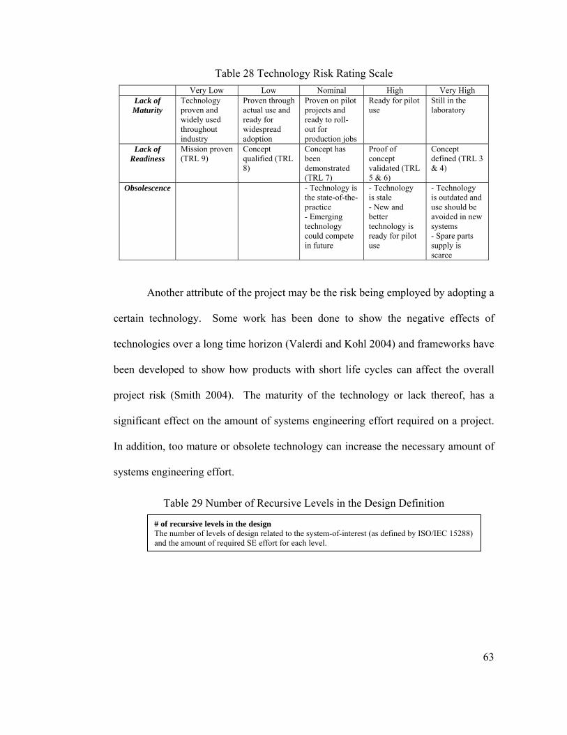
63
Table 28 Technology Risk Rating Scale Very Low Low Nominal High Very High
Lack of Maturity
Technology proven and widely used throughout industry
Proven through actual use and ready for widespread adoption
Proven on pilot projects and ready to roll-out for production jobs
Ready for pilot use
Still in the laboratory
Lack of Readiness
Mission proven (TRL 9)
Concept qualified (TRL 8)
Concept has been demonstrated (TRL 7)
Proof of concept validated (TRL 5 & 6)
Concept defined (TRL 3 & 4)
Obsolescence - Technology is the state-of-the-practice - Emerging technology could compete in future
- Technology is stale - New and better technology is ready for pilot use
- Technology is outdated and use should be avoided in new systems - Spare parts supply is scarce
Another attribute of the project may be the risk being employed by adopting a
certain technology. Some work has been done to show the negative effects of
technologies over a long time horizon (Valerdi and Kohl 2004) and frameworks have
been developed to show how products with short life cycles can affect the overall
project risk (Smith 2004). The maturity of the technology or lack thereof, has a
significant effect on the amount of systems engineering effort required on a project.
In addition, too mature or obsolete technology can increase the necessary amount of
systems engineering effort.
Table 29 Number of Recursive Levels in the Design Definition
# of recursive levels in the design The number of levels of design related to the system-of-interest (as defined by ISO/IEC 15288) and the amount of required SE effort for each level.
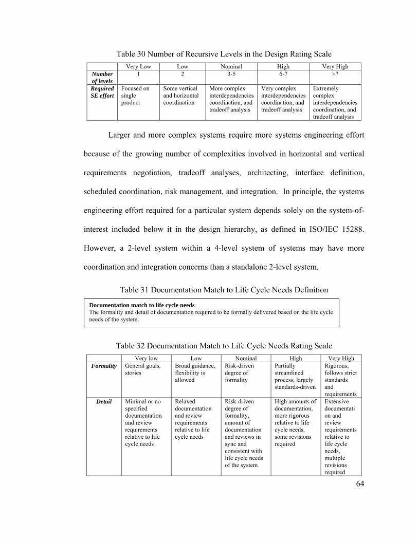
64
Table 30 Number of Recursive Levels in the Design Rating Scale Very Low Low Nominal High Very High
Number of levels
1 2 3-5 6-7 >7
Required SE effort
Focused on single product
Some vertical and horizontal coordination
More complex interdependencies coordination, and tradeoff analysis
Very complex interdependencies coordination, and tradeoff analysis
Extremely complex interdependencies coordination, and tradeoff analysis
Larger and more complex systems require more systems engineering effort
because of the growing number of complexities involved in horizontal and vertical
requirements negotiation, tradeoff analyses, architecting, interface definition,
scheduled coordination, risk management, and integration. In principle, the systems
engineering effort required for a particular system depends solely on the system-of-
interest included below it in the design hierarchy, as defined in ISO/IEC 15288.
However, a 2-level system within a 4-level system of systems may have more
coordination and integration concerns than a standalone 2-level system.
Table 31 Documentation Match to Life Cycle Needs Definition
Table 32 Documentation Match to Life Cycle Needs Rating Scale Very low Low Nominal High Very High
Formality General goals, stories
Broad guidance, flexibility is allowed
Risk-driven degree of formality
Partially streamlined process, largely standards-driven
Rigorous, follows strict standards and requirements
Detail Minimal or no specified documentation and review requirements relative to life cycle needs
Relaxed documentation and review requirements relative to life cycle needs
Risk-driven degree of formality, amount of documentation and reviews in sync and consistent with life cycle needs of the system
High amounts of documentation, more rigorous relative to life cycle needs, some revisions required
Extensive documentation and review requirements relative to life cycle needs, multiple revisions required
Documentation match to life cycle needs The formality and detail of documentation required to be formally delivered based on the life cycle needs of the system.
65
Some system products require large amounts of documentation. The
importance and enforcement of this requirement is often related to the type of system
being developed and the nature of the system’s users, operators, and maintainers.
Less documentation is needed when the users and operators are expert and stable,
and the developers become the maintainers. The importance of this factor, then, is
based on the match or mismatch of documentation requirements to the life cycle
needs of the system. Attempting to save costs via very low or low documentation
levels will generally incur extra costs during the maintenance portion of the life cycle.
Poor or missing documentation can also cause additional problems in other stages of
the life cycle. This driver includes two dimensions, formality and detail, to represent
the different aspects of documentation that need to be considered. A nominal rating
involves documentation consistent with life cycle needs. Its degree of formality and
detail are risk-driven; if it is low risk not to include something, it is not included.
3.3.3. Operations Factors
The operations factors refer to the hardware and software environments that a
system will operate within. Depending on the system of interest, the platform might
be an aircraft carrier; an aircraft; an airborne missile; a navigation, guidance, and
control system; or a level of the computer system’s software infrastructure. The
existence of legacy issues may also impact the amount of systems engineering effort
required to incorporate the new system with existing technologies and cultures.
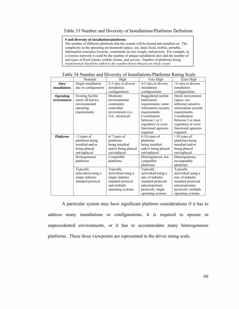
66
Table 33 Number and Diversity of Installations/Platforms Definition
Table 34 Number and Diversity of Installations/Platforms Rating Scale Nominal High Very High Extra High
Sites/ installations
Single installation site or configuration
2-3 sites or diverse installation configurations
4-5 sites or diverse installation configurations
>6 sites or diverse installation configurations
Operating environment
Existing facility meets all known environmental operating requirements
Moderate environmental constraints; controlled environment (i.e., A/C, electrical)
Ruggedized mobile land-based requirements; some information security requirements. Coordination between 1 or 2 regulatory or cross functional agencies required.
Harsh environment (space, sea airborne) sensitive information security requirements. Coordination between 3 or more regulatory or cross functional agencies required.
<3 types of platforms being installed and/or being phased out/replaced
4-7 types of platforms being installed and/or being phased out/replaced
8-10 types of platforms being installed and/or being phased out/replaced
>10 types of platforms being installed and/or being phased out/replaced
Homogeneous platforms
Compatible platforms
Heterogeneous, but compatible platforms
Heterogeneous, incompatible platforms
Platforms
Typically networked using a single industry standard protocol
Typically networked using a single industry standard protocol and multiple operating systems
Typically networked using a mix of industry standard protocols and proprietary protocols; single operating systems
Typically networked using a mix of industry standard protocols and proprietary protocols; multiple operating systems
A particular system may have significant platform considerations if it has to
address many installations or configurations, it is required to operate in
unprecedented environments, or it has to accommodate many heterogeneous
platforms. These three viewpoints are represented in the driver rating scale.
# and diversity of installations/platforms The number of different platforms that the system will be hosted and installed on. The complexity in the operating environment (space, sea, land, fixed, mobile, portable, information assurance/security, constraints on size weight, and power). For example, in a wireless network it could be the number of unique installation sites and the number of and types of fixed clients, mobile clients, and servers. Number of platforms being implemented should be added to the number being phased out (dual count).
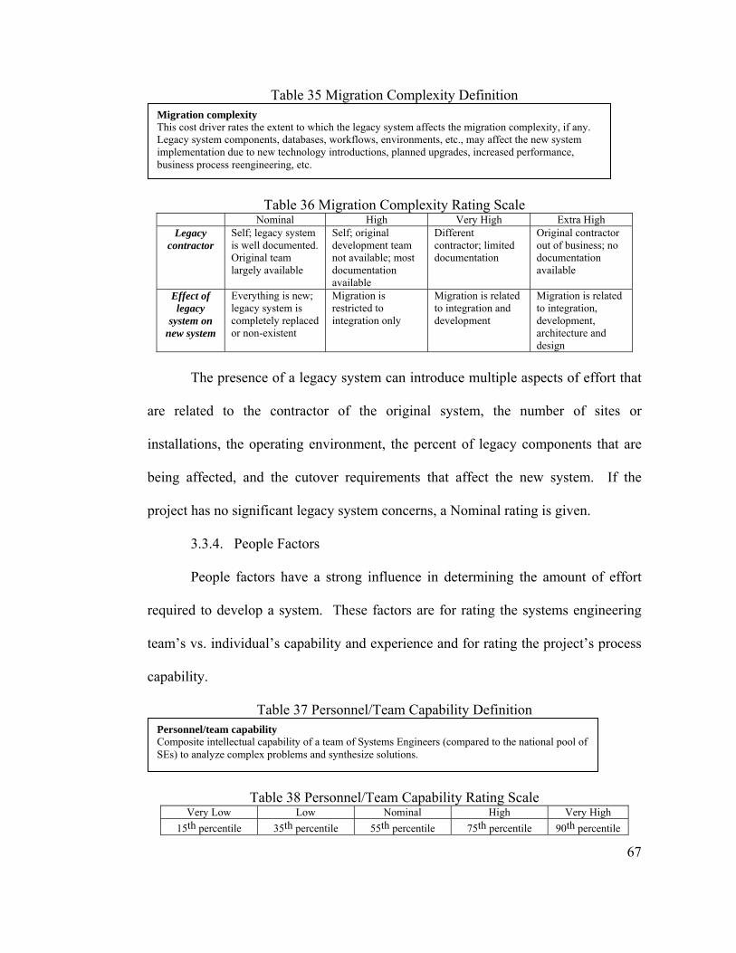
67
Table 35 Migration Complexity Definition
Table 36 Migration Complexity Rating Scale Nominal High Very High Extra High
Legacy contractor
Self; legacy system is well documented. Original team largely available
Self; original development team not available; most documentation available
Different contractor; limited documentation
Original contractor out of business; no documentation available
Effect of legacy
system on new system
Everything is new; legacy system is completely replaced or non-existent
Migration is restricted to integration only
Migration is related to integration and development
Migration is related to integration, development, architecture and design
The presence of a legacy system can introduce multiple aspects of effort that
are related to the contractor of the original system, the number of sites or
installations, the operating environment, the percent of legacy components that are
being affected, and the cutover requirements that affect the new system. If the
project has no significant legacy system concerns, a Nominal rating is given.
3.3.4. People Factors
People factors have a strong influence in determining the amount of effort
required to develop a system. These factors are for rating the systems engineering
team’s vs. individual’s capability and experience and for rating the project’s process
capability.
Table 37 Personnel/Team Capability Definition
Table 38 Personnel/Team Capability Rating Scale Very Low Low Nominal High Very High
15th percentile 35th percentile 55th percentile 75th percentile 90th percentile
Personnel/team capability Composite intellectual capability of a team of Systems Engineers (compared to the national pool of SEs) to analyze complex problems and synthesize solutions.
Migration complexity This cost driver rates the extent to which the legacy system affects the migration complexity, if any. Legacy system components, databases, workflows, environments, etc., may affect the new system implementation due to new technology introductions, planned upgrades, increased performance, business process reengineering, etc.
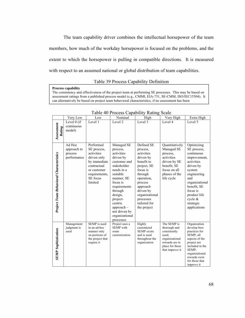
68
The team capability driver combines the intellectual horsepower of the team
members, how much of the workday horsepower is focused on the problems, and the
extent to which the horsepower is pulling in compatible directions. It is measured
with respect to an assumed national or global distribution of team capabilities.
Table 39 Process Capability Definition
Table 40 Process Capability Rating Scale Very Low Low Nominal High Very High Extra High
Ass
essm
ent
Rat
ing
Level 0 (if continuous model)
Level 1 Level 2 Level 3 Level 4 Level 5
Proj
ect T
eam
Beh
avio
ral C
hara
cter
istic
s
Ad Hoc approach to process performance
Performed SE process, activities driven only by immediate contractual or customer requirements, SE focus limited
Managed SE process, activities driven by customer and stakeholder needs in a suitable manner, SE focus is requirements through design, project-centric approach – not driven by organizational processes
Defined SE process, activities driven by benefit to project, SE focus is through operation, process approach driven by organizational processes tailored for the project
Quantitatively Managed SE process, activities driven by SE benefit, SE focus on all phases of the life cycle
Optimizing SE process, continuous improvement, activities driven by system engineering and organizational benefit, SE focus is product life cycle & strategic applications
SEM
P So
phis
ticat
ion
Management judgment is used
SEMP is used in an ad-hoc manner only on portions of the project that require it
Project uses a SEMP with some customization
Highly customized SEMP exists and is used throughout the organization
The SEMP is thorough and consistently used; organizational rewards are in place for those that improve it
Organization develop best practices for SEMP; all aspects of the project are included in the SEMP; organizational rewards exist for those that improve it
Process capability The consistency and effectiveness of the project team at performing SE processes. This may be based on assessment ratings from a published process model (e.g., CMMI, EIA-731, SE-CMM, ISO/IEC15504). It can alternatively be based on project team behavioral characteristics, if no assessment has been
69
The procedure for determining a project’s systems engineering process
capability is organized around the Software Engineering Institute’s Capability
Maturity Model Integration® (CMMI). The time period for rating process capability
is the time the project starts, and should be a reflection of the project only – not of
the total organization’s maturity level. There are two methods of rating process
capability. The first captures the CMMI® continuous model (CMMI 2002; Shrum
2000) and the systems engineering maturity model EIA 731 (ANSI/EIA 2002). The
second combines the degrees of mastery of each process area as done for the
software CMM in COCOMO II (Clark 1997; Boehm et al 2000). Only the first
method is employed here. The project team behavioral characteristics are somewhat
analogous to the CMMI levels and can be used by organizations that do not use
CMMI ratings. The final viewpoint captures levels of sophistication of the Systems
Engineering Management Plan. The higher the sophistication of this document, the
higher the systems engineering effort savings because the level of planning
associated with a SEMP is indicative of well-managed systems engineering
processes.
3.3.5. Environment Factors
The environment factors capture the sophistication of the systems
engineering environment in a project. Coordination and support are the two drivers
that make up this theme.
Table 41 Multisite Coordination Definition
Multisite coordination Location of stakeholders, team members, resources, corporate collaboration barriers.
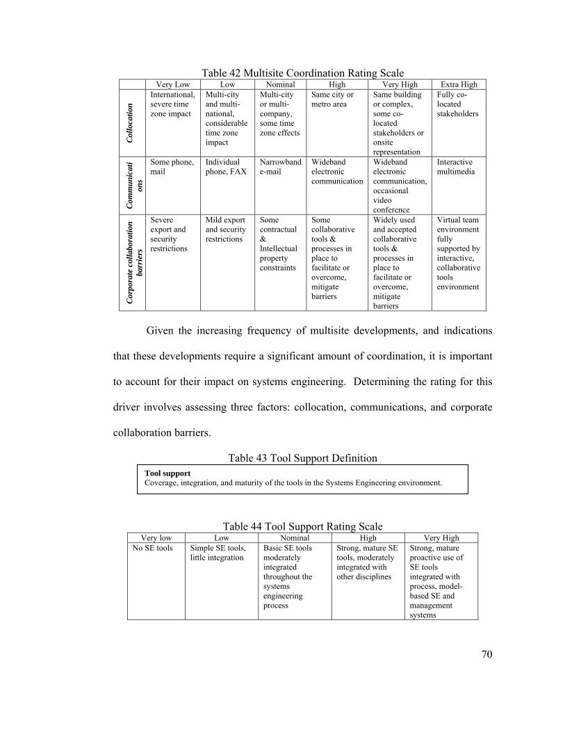
70
Table 42 Multisite Coordination Rating Scale Very Low Low Nominal High Very High Extra High
Col
loca
tion
International, severe time zone impact
Multi-city and multi-national, considerable time zone impact
Multi-city or multi-company, some time zone effects
Same city or metro area
Same building or complex, some co-located stakeholders or onsite representation
Fully co-located stakeholders
Com
mun
icat
ion
s
Some phone, mail
Individual phone, FAX
Narrowband e-mail
Wideband electronic communication
Wideband electronic communication, occasional video conference
Interactive multimedia
Cor
pora
te c
olla
bora
tion
barr
iers
Severe export and security restrictions
Mild export and security restrictions
Some contractual & Intellectual property constraints
Some collaborative tools & processes in place to facilitate or overcome, mitigate barriers
Widely used and accepted collaborative tools & processes in place to facilitate or overcome, mitigate barriers
Virtual team environment fully supported by interactive, collaborative tools environment
Given the increasing frequency of multisite developments, and indications
that these developments require a significant amount of coordination, it is important
to account for their impact on systems engineering. Determining the rating for this
driver involves assessing three factors: collocation, communications, and corporate
collaboration barriers.
Table 43 Tool Support Definition
Table 44 Tool Support Rating Scale Very low Low Nominal High Very High
No SE tools Simple SE tools, little integration
Basic SE tools moderately integrated throughout the systems engineering process
Strong, mature SE tools, moderately integrated with other disciplines
Strong, mature proactive use of SE tools integrated with process, model-based SE and management systems
Tool support Coverage, integration, and maturity of the tools in the Systems Engineering environment.
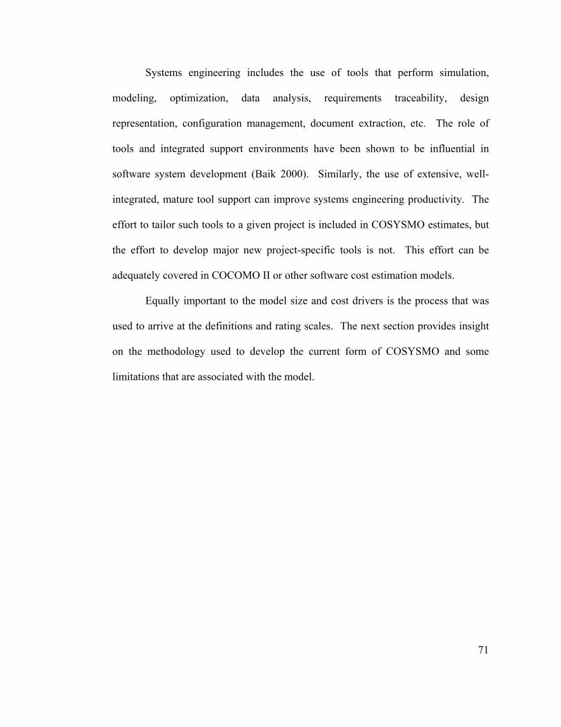
71
Systems engineering includes the use of tools that perform simulation,
modeling, optimization, data analysis, requirements traceability, design
representation, configuration management, document extraction, etc. The role of
tools and integrated support environments have been shown to be influential in
software system development (Baik 2000). Similarly, the use of extensive, well-
integrated, mature tool support can improve systems engineering productivity. The
effort to tailor such tools to a given project is included in COSYSMO estimates, but
the effort to develop major new project-specific tools is not. This effort can be
adequately covered in COCOMO II or other software cost estimation models.
Equally important to the model size and cost drivers is the process that was
used to arrive at the definitions and rating scales. The next section provides insight
on the methodology used to develop the current form of COSYSMO and some
limitations that are associated with the model.
72
4. Methodology
4.1. Research Design & Data Collection
The previous sections outlined the need for COSYSMO and outlined the
details of the individual drivers that affect systems engineering. The next steps in
developing a useful model involve (1) the identification of the appropriate research
designs and approaches; and (2) the correct application of these methods to the
research question.
Historically, research in the behavioral sciences goes back to the emergence
of psychology as a scientific discipline in the 1800’s. As psychology matured, it
evolved into a collection of methodologies which included scientific inquiry,
measurement, and data analysis (Freud 1924). Branches of psychology emerged and
provided different analytical techniques which incorporated statistical models and
experimental techniques (Berne 1964). Other behavior-oriented fields such as
sociology have contributed much in the sense of formal research methods and
research design (Babbie 2004). The field of education has provided frameworks for
categorizing different types of research designs, methods, and strategies (Isaac and
Michael 1997). In this light, the research approach adopted for this work is a
combination of field research and quasi-experimental research. The nature of the
research question – how to estimate systems engineering – played the major role in
determining the selection of these approaches.
Research Design. The purpose of field research design is to study the
background, current status, and environmental interactions of a given social unit.
73
The social units of interest are organizations that develop large-scale technology
enabled systems and the systems engineers that work on them. The expert data that
has been collected through the Delphi survey attempts to capture project phenomena
to help understand the role of systems engineering in an organization. The strengths
of this method are that it provides:
• an in-depth investigation of systems engineering organizations
• useful anecdotes or examples to illustrate more generalized statistical
findings
• observations of real world phenomena and opportunities to incorporate
them into theory
The purpose of quasi-experimental research design is to approximate the
conditions of the true experiment in a setting that does not allow control or
manipulation of all relevant variables. The multiple factors that affect the conditions
can compromise the validity of the design. Since the desired social unit – the
systems engineering organization – is influenced by multiple outside forces such as
corporate culture, customer pressures, financial priorities, employment challenges,
and technical obstacles, it is nearly impossible to control all of the conditions.
However, this method is useful because it allows for:
• investigation of cause-and-effect relationships
• variance of different type of projects operating under different conditions
• opportunity to test specific hypotheses
Combining the strengths of field research and quasi-experimental research
provides significant benefits because they use different perspectives in the data
74
collection process. Having the right frame of mind while defining the hypotheses
and then testing them is also extremely important. During the development of
COSYSMO, two different research approaches were adopted: interpretivist and
positivist. These two techniques provide fundamentally different approaches at
gathering data and validating it, but using them at different stages of the research
process can enable a more complete study (Klein and Myers 1999).
Research Approach. The interpretivist approach focuses on the complexity
of human sense making as the situation emerges. It enables researchers to learn as
much as possible about the phenomena being studied and arrive at qualitative
conclusions as to the most important factors. The interpretivist approach was used
when developing the size and cost driver definitions with USC corporate affiliates.
Through a series of interviews, surveys, and working group meetings the
identification and definition of the most significant size and cost drivers was
accomplished. The three criteria for the interpretivist approach are:
• Credibility – establishing a match between the constructed realities of
systems engineering and the respondents or stakeholders
• Transferability – presenting sufficiently detailed systems engineering cost
drivers as to enable judgment that these findings can be transferred to
other contexts
• Confirmability – Ensuring that the size and cost drivers are grounded in
systems engineering theory and not just a result of the researcher’s
imagination
75
Once the systems engineering drivers were defined, there was a shift in the
research strategy to a positivist approach. The positivist approach focuses on making
formal propositions, quantifiable measures of variables, hypothesis testing, and the
drawing of inferences about a phenomenon from a representative sample to a stated
population. The criteria associated with this approach are:
• Construct validity – establishing the right operational measures for
systems engineering size and cost
• Internal validity – establishing causal relationships between the drivers
and systems engineering effort
• External validity – establishing the domain to which the systems
engineering drivers can be generalized
• Reliability – ensuring that the relationships between the size and cost
drivers can be repeated with the same results
These are discussed in more detail in Chapter 5. The shift from interpretivist
to positivist is analogous to a qualitative to quantitative shift in research. While the
beginning of the model building process required an open mind about the
relationships between the size and cost drivers to effort, the latter part of the process
involved testing the hypotheses previously defined and determining their suitability
to the research questions. Using both of these approaches increases the chances of
obtaining interesting findings.
The two research approaches and two strategies were applied to the same
methodology used to develop the COCOMO model. This proven model
development process is outlined in the book Software Cost Estimation With
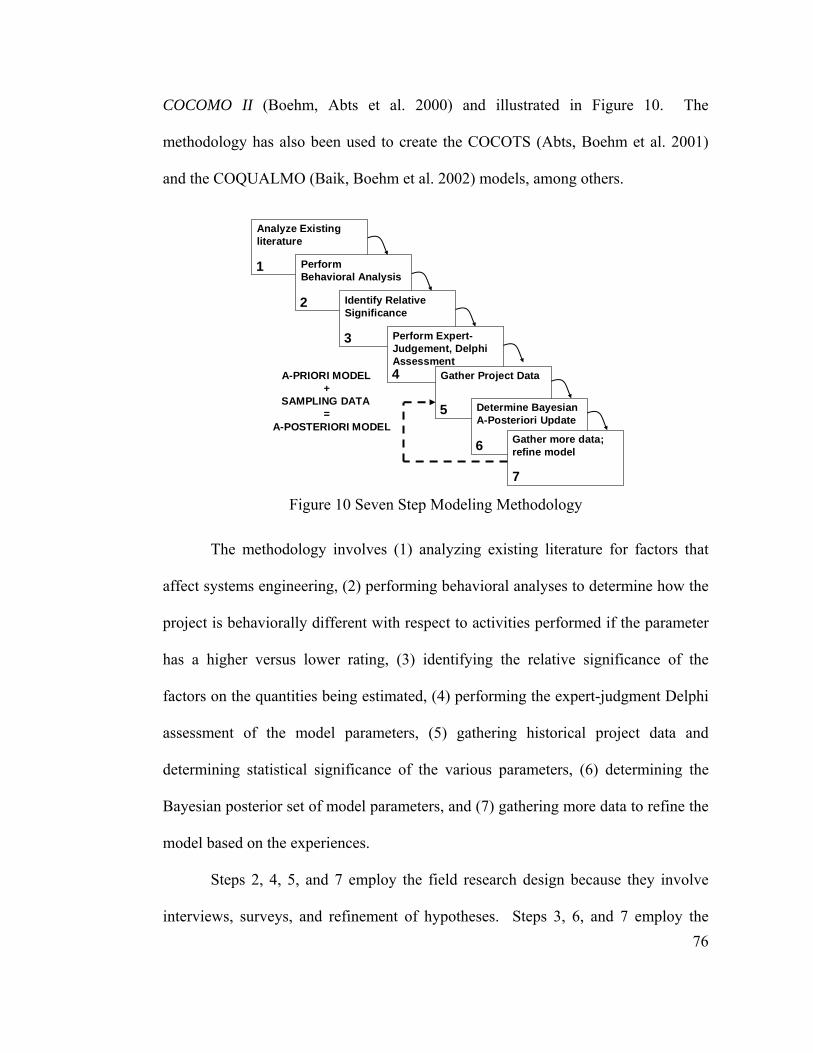
76
COCOMO II (Boehm, Abts et al. 2000) and illustrated in Figure 10. The
methodology has also been used to create the COCOTS (Abts, Boehm et al. 2001)
and the COQUALMO (Baik, Boehm et al. 2002) models, among others.
Analyze Existingliterature
1
2
3
4
5
6
7
PerformBehavioral Analysis
Identify RelativeSignificance
Perform Expert-Judgement, DelphiAssessment
Gather Project Data
Determine BayesianA-Posteriori Update
Gather more data;refine model
A-PRIORI MODEL+
SAMPLING DATA=
A-POSTERIORI MODEL
Figure 10 Seven Step Modeling Methodology
The methodology involves (1) analyzing existing literature for factors that
affect systems engineering, (2) performing behavioral analyses to determine how the
project is behaviorally different with respect to activities performed if the parameter
has a higher versus lower rating, (3) identifying the relative significance of the
factors on the quantities being estimated, (4) performing the expert-judgment Delphi
assessment of the model parameters, (5) gathering historical project data and
determining statistical significance of the various parameters, (6) determining the
Bayesian posterior set of model parameters, and (7) gathering more data to refine the
model based on the experiences.
Steps 2, 4, 5, and 7 employ the field research design because they involve
interviews, surveys, and refinement of hypotheses. Steps 3, 6, and 7 employ the
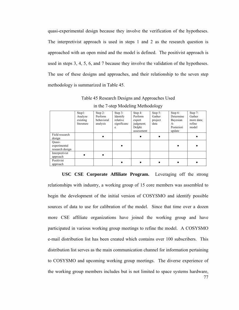
77
quasi-experimental design because they involve the verification of the hypotheses.
The interpretivist approach is used in steps 1 and 2 as the research question is
approached with an open mind and the model is defined. The positivist approach is
used in steps 3, 4, 5, 6, and 7 because they involve the validation of the hypotheses.
The use of these designs and approaches, and their relationship to the seven step
methodology is summarized in Table 45.
Table 45 Research Designs and Approaches Used
in the 7-step Modeling Methodology Step1:
Analyze existing literature
Step 2: Perform behavioral analysis
Step 3: Identify relative significance
Step 4: Perform expert judgment; Delphi assessment
Step 5: Gather project data
Step 6: Determine Bayesian A-Posteriori update
Step 7: Gather more data; refine model
Field research design ● ● ● ●
Quasi-experimental research design
● ● ●
Interpretivist approach ● ●
Positivist approach ● ● ● ● ●
USC CSE Corporate Affiliate Program. Leveraging off the strong
relationships with industry, a working group of 15 core members was assembled to
begin the development of the initial version of COSYSMO and identify possible
sources of data to use for calibration of the model. Since that time over a dozen
more CSE affiliate organizations have joined the working group and have
participated in various working group meetings to refine the model. A COSYSMO
e-mail distribution list has been created which contains over 100 subscribers. This
distribution list serves as the main communication channel for information pertaining
to COSYSMO and upcoming working group meetings. The diverse experience of
the working group members includes but is not limited to space systems hardware,
78
information technology, radars, satellite ground stations, and military aircraft. This
broad scope helps ensure that the model is robust enough to address multiple areas.
The typical involvement of affiliate companies is twofold. First, each
company provides a group of systems engineering experts to rate the model drivers
through the use of a wideband Delphi survey. This exercise allows for expert
judgement to be captured and included in the model. An additional source of
expertise has been the members of INCOSE who have provided extensive valuable
feedback that has greatly improved the model. Second, the Affiliate companies
provide historical project data for the COSYSMO calibration to validate the model
parameters. This ensures that the Cost Estimating Relationships (CERs) in the
model are appropriately weighed according to the data received from completed
projects.
Need for industry data to calibrate COSYSMO. Industrial participation in
the development of COSYSMO is key to the usefulness and relevance of the model.
Each driver has a corresponding item that can provide the necessary data for the
calibration. The initial industry calibration is essential to understanding the model’s
robustness, establishing initial relationships between parameters and outcomes, and
determining the validity of drivers. However, each organization using COSYSMO
will need to perform a local calibration. Through the industry calibration, the
working group can establish the values for various scale factors for each driver. This
might not be possible or feasible from a local calibration due to the size of the
calibration data set and the narrow scope of a single organization’s project database.
The industry data can also identify elements or features of the model that need
79
refinement. Obtaining data from multiple sources may also identify new drivers that
need to be included in future revisions of the model.
An additional important reason for an industry-level calibration is the
acceptance of the model for cost estimation by the Defense Contract Audit Agency
(DCAA). Even though each organization needs to prove the local calibration
matches the local organization's productivity and trends, the industry calibration
shows DCAA the model meets the expectations and standards of the Systems
Engineering industry. Ensuring that COSYSMO is compatible with these standards
plays an important role in its widespread acceptance and generalizability.
Data Collection. The collection of data itself, steps 4, 5, and 7, can be
divided into two unique efforts: one focusing on expert data and the other on
historical project data. The process used for collecting expert data, the Delphi
technique (Dalkey 1969) is performed in Step 4. Developed at The RAND
Corporation in the late 1940s, it serves as a way of making predictions about future
events - thus its name, recalling the divinations of the Greek oracle of antiquity,
located on the southern flank of Mt. Parnassus at Delphi (Ahern, Clouse et al. 2004).
More recently, the technique has been used as a means of guiding a group of
informed individuals to a consensus of opinion on some issue.
Participants are asked to make an assessment regarding the ratings of size and
cost drivers, individually in a preliminary round, without consulting the other
participants in the exercise. The first round results are then collected, tabulated, and
returned to each participant for a second round, during which the participants are
again asked to make an assessment regarding the same issue. The second time
80
around the participants had the knowledge of what the other participants responded
in the first round. The second round usually results in a narrowing of the range in
assessments by the group, pointing to some reasonable middle ground regarding the
issue of concern. The original Delphi technique avoided group discussion; but the
Wideband Delphi technique (Boehm 1981) accommodated group discussion between
assessment rounds. Two rounds of the Wideband Delphi survey for COSYSMO
have been completed. The results are shown in the next section.
The second data collection effort involves steps 5 and 7. One completed
project with an accurate count of systems engineering hours is considered one data
point. These projects have been contributed by CSE Affiliates that wish to have their
application domains considered in the model. To date, eleven projects have been
submitted to the COSYSMO repository for analysis.
Measurement reliability. An important experimental issue in field and
quasi-experimental research designs is that of measurement reliability (Jarvenpaa,
Dickson et al. 1985). This refers to the possible errors in measurement due to the
accuracy of the measurement instrument. Surveys were used for both the Delphi and
historical project data. Careful steps were taken to ensure that the design of the
survey instrument followed the best practices in questionnaire design (Sudman and
Bradburn 1982). Some of these are:
• Use of closed and open ended questions
• Knowledge questions to screen out respondents who lack sufficient
information
• Consistent measurement scales for all questions of the same type
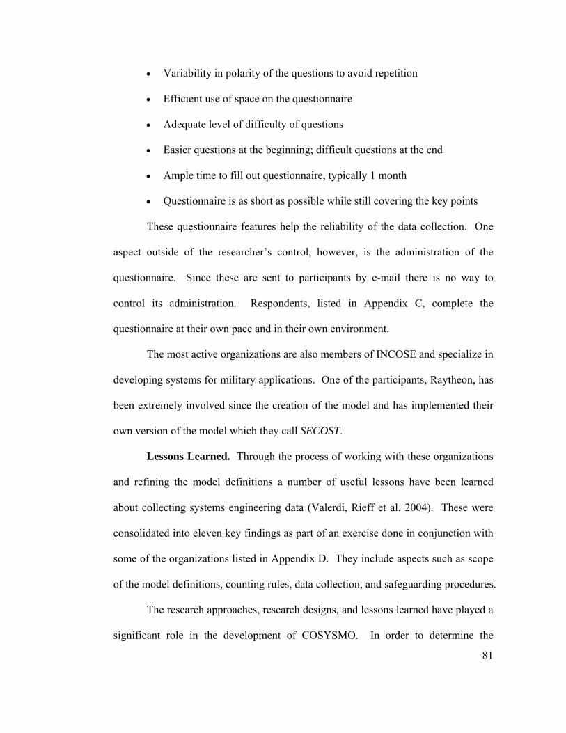
81
• Variability in polarity of the questions to avoid repetition
• Efficient use of space on the questionnaire
• Adequate level of difficulty of questions
• Easier questions at the beginning; difficult questions at the end
• Ample time to fill out questionnaire, typically 1 month
• Questionnaire is as short as possible while still covering the key points
These questionnaire features help the reliability of the data collection. One
aspect outside of the researcher’s control, however, is the administration of the
questionnaire. Since these are sent to participants by e-mail there is no way to
control its administration. Respondents, listed in Appendix C, complete the
questionnaire at their own pace and in their own environment.
The most active organizations are also members of INCOSE and specialize in
developing systems for military applications. One of the participants, Raytheon, has
been extremely involved since the creation of the model and has implemented their
own version of the model which they call SECOST.
Lessons Learned. Through the process of working with these organizations
and refining the model definitions a number of useful lessons have been learned
about collecting systems engineering data (Valerdi, Rieff et al. 2004). These were
consolidated into eleven key findings as part of an exercise done in conjunction with
some of the organizations listed in Appendix D. They include aspects such as scope
of the model definitions, counting rules, data collection, and safeguarding procedures.
The research approaches, research designs, and lessons learned have played a
significant role in the development of COSYSMO. In order to determine the
82
predictive power of the model it has been validated through the use of statistical
techniques. This effort represents step 5 of the seven step modeling methodology
and is discussed in detail in the next section. One of the most human-intensive
portions of this work was obtaining data from aerospace companies. The principal
activities associated with the process of obtaining data from companies are illustrated
in Figure 11.
Figure 11 Data Handshaking
4.2. Threats to Validity & Limitations
Two types of threats to validity exist: controllable and uncontrollable. Great
care has been taken to make sure COSYSMO is a useful model for systems
engineering effort. Experimental design, however, is not perfect. Many external
factors can affect the experiment and influence the overall result. This section
attempts to identify the most significant threats to the validity of COSYSMO and
outlines ways in which they were reduced. Most of these relate to external validity;
the ability to generalize findings to other settings. Consequently, a COSYSMO user
83
may ask: To what size or type of systems engineering projects can the model be
generalized? The external validity of an experiment can be strengthened by
describing the population to which the results will apply before the model is used. If
a random systems engineering project is selected from a predetermined population
(i.e, satellite ground stations) and COSYSMO yields an accurate estimate for
systems engineering then the generalization can be made that systems engineering
can be estimated with a certain degree of accuracy for satellite ground stations.
The data variability that is obtained from the data collection will determine
how extensively the findings can be applied. If the model is calibrated from projects
for military or defense applications, it cannot be claimed that the systems
engineering CERs will hold true for other types of projects. The controllable threats
to validity are:
1. Construct validity. The ensemble of size and cost drivers was carefully
selected and tested to ensure that they were indeed adequate measures of
systems engineering. They were also verified with heuristics, previous
studies, and expert opinion.
2. Construct reliability. Counting rules and definitions were developed, with
industry feedback, to guard against possible multiple interpretations and
ensure consistent use of the drivers throughout different systems engineering
domains.
3. Divergent definitions of Systems Engineering. An industry-accepted
standard was adopted (EIA/ANSI 632) to aid in the identification of systems
engineering activities through a baseline Work Breakdown Structure.
84
4. Experts. Expert sampling involves the assembling of a sample of persons
with known or demonstrable experience and expertise in some area. Often,
we convene such a sample under the auspices of a "panel of experts." There
are actually two reasons one might do expert sampling. First, because it
would be the best way to elicit the views of persons who have specific
expertise. Second, because the expert sampling might be used to provide
evidence for the validity of another sampling approach. For instance, the
systems engineering drivers defined in COSYSMO need to be field tested by
future users of the model. A panel of experts with experience and insight into
systems engineering can examine the definitions and determine their
appropriateness and validity. The advantage of doing this is that the drivers
have significant practical relevance. The disadvantage is that even the
experts can be, and often are, wrong. The responses in the Delphi survey
came from “experts” in the field of systems engineering but the method used
to administer the survey (e-mail) did not allow for screening of the survey
respondents. To control for this, a set of questions was included at the
beginning of the survey that asked respondents for their years of experience
in systems engineering and/or cost estimation. The purpose of the question
was to allow for the respondents to self select if they did not feel their
experience was adequate to respond to the survey.
Other threats to validity exist which were identified but uncontrollable
because they are often outside the range of control of the researcher. They may be
the main source of error in the model since their impact is difficult to quantify:
85
1. Noisy data. Significant effort reporting differences and partial size
information (i.e., size factor volatility and reuse) introduced some error in the
data.
2. Nonresponse bias. Case study research is limited in its representativeness.
The sample that is currently being used to calibrate COSYSMO is limited to
the companies that have shown interest and made it possible to contribute
systems engineering data or have been able to respond to the Delphi surveys.
Because of the narrow focus on only a few projects, there is a limitation to
the model’s generalizability because it only represents the CERs that are
confirmed by the data set in use. Attempts have been made to include
INCOSE and non-INCOSE companies that use systems engineering but only
aerospace and defense companies affiliated with INCOSE were responsive.
Moreover, these companies often exhibited a CMMI rating of 3 or higher;
biasing the results towards high maturity organizations.
3. Sample Self-selection. This dissertation involved the collection of data from
six defense companies and the solicitation of inputs from experts employed at
these companies which, in some cases, represent heterogeneous cultures due
to the consolidation of the aerospace industry. Some of these companies
have acquired portions of each other. As a result, a single aerospace
company may reflect diverse cultural, productivity, and process standards
inherited from all or portions of heritage companies it has acquired or merged
with as shown in Table 46.
Table 46 Consolidation of Aerospace Companies
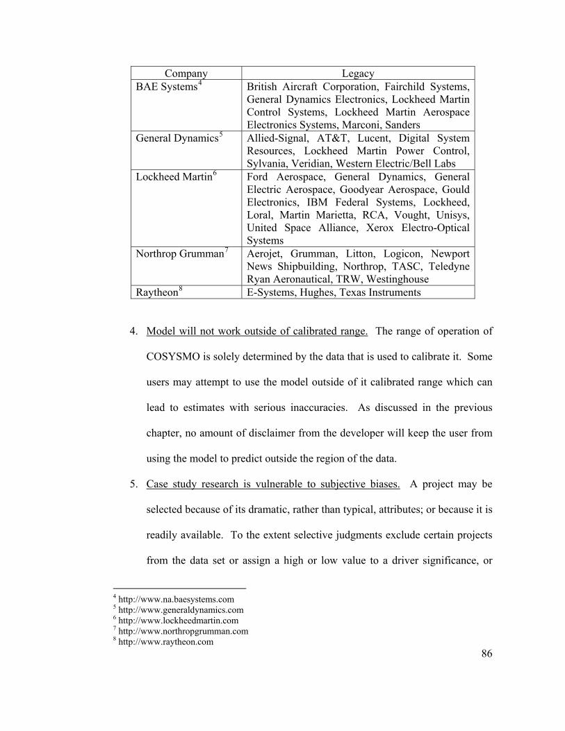
86
Company Legacy BAE Systems4 British Aircraft Corporation, Fairchild Systems,
General Dynamics Electronics, Lockheed Martin Control Systems, Lockheed Martin Aerospace Electronics Systems, Marconi, Sanders
General Dynamics5 Allied-Signal, AT&T, Lucent, Digital System Resources, Lockheed Martin Power Control, Sylvania, Veridian, Western Electric/Bell Labs
Lockheed Martin6 Ford Aerospace, General Dynamics, General Electric Aerospace, Goodyear Aerospace, Gould Electronics, IBM Federal Systems, Lockheed, Loral, Martin Marietta, RCA, Vought, Unisys, United Space Alliance, Xerox Electro-Optical Systems
Northrop Grumman7 Aerojet, Grumman, Litton, Logicon, Newport News Shipbuilding, Northrop, TASC, Teledyne Ryan Aeronautical, TRW, Westinghouse
Raytheon8 E-Systems, Hughes, Texas Instruments
4. Model will not work outside of calibrated range. The range of operation of
COSYSMO is solely determined by the data that is used to calibrate it. Some
users may attempt to use the model outside of it calibrated range which can
lead to estimates with serious inaccuracies. As discussed in the previous
chapter, no amount of disclaimer from the developer will keep the user from
using the model to predict outside the region of the data.
5. Case study research is vulnerable to subjective biases. A project may be
selected because of its dramatic, rather than typical, attributes; or because it is
readily available. To the extent selective judgments exclude certain projects
from the data set or assign a high or low value to a driver significance, or
4 http://www.na.baesystems.com 5 http://www.generaldynamics.com 6 http://www.lockheedmartin.com 7 http://www.northropgrumman.com 8 http://www.raytheon.com
87
place them in one context rather than another, subjective interpretation is
influencing the outcome. Moreover, only successful projects are reported for
inclusion in COSYSMO. This makes the model biased towards successful
projects because the unsuccessful projects do not collect or share data and are
not included in the calibration.
6. Difficult to identify external variables. In quasi-experimental research it is
difficult to identify all non-experimental project variables (i.e., competitive
pressures, market trends, strategic advantages, etc.) and determine how to
control or account for them.
7. Telescoping. The historical project data collection survey requires the
respondent to go back in time and investigate the qualitative and quantitative
parameters of the project. The quantitative parameters may be found in
project documentation, if available. But the qualitative parameters will
require a systems engineer or program manager to recollect a time frame in
the past, referred to as telescoping. This technique has obvious drawbacks
because individuals may not remember everything that happened in the past
or they may be formulating their responses from secondary references. To
overcome this, the focus is on obtaining historical project data on recently
completed projects to increase the probability of accurate information and
knowledgeable personnel with first hand experience.
8. Group Conformity. Solomon Asch's most famous experiments set a contest
between physical and social reality. His subjects judged unambiguous stimuli
– lines of different lengths – after hearing other opinions offering incorrect
88
estimates. Subjects were very upset by the discrepancy between their
perceptions and those of others and most caved under the pressure to
conform: only 29% of his subjects refused to join the bogus majority. In a
similar way, systems engineers could fall into the same trap and agree with
incorrect estimates based on what the group thinks is the correct choice.
With these threats in mind, a number of limitations also exist. The
application domain profile of the application domain of Delphi survey respondents is
shown in Figure 12. Nine out of forty (22%) participants who participated in Round
1 also took part in Round 2. To control for unfamiliarity of parametric models,
follow up interviews were held with experts whose responses were outliers to get
clarification on their answers. The average years of experience in software or
systems engineering of survey participants was 18 years and the average years of
experience in cost modeling was 6 years. Employees from fourteen different
organizations participated in the survey but the majority (55%) of the participants
were employees of Raytheon, Lockheed Martin, and Northrop Grumman. Proceed
with caution if either (1) you are not one of the six companies that provided data, (2)
your systems are outside of the size range for which the model is calibrated, and (3)
your definition of systems engineering is not compatible with ANSI/EIA 632.
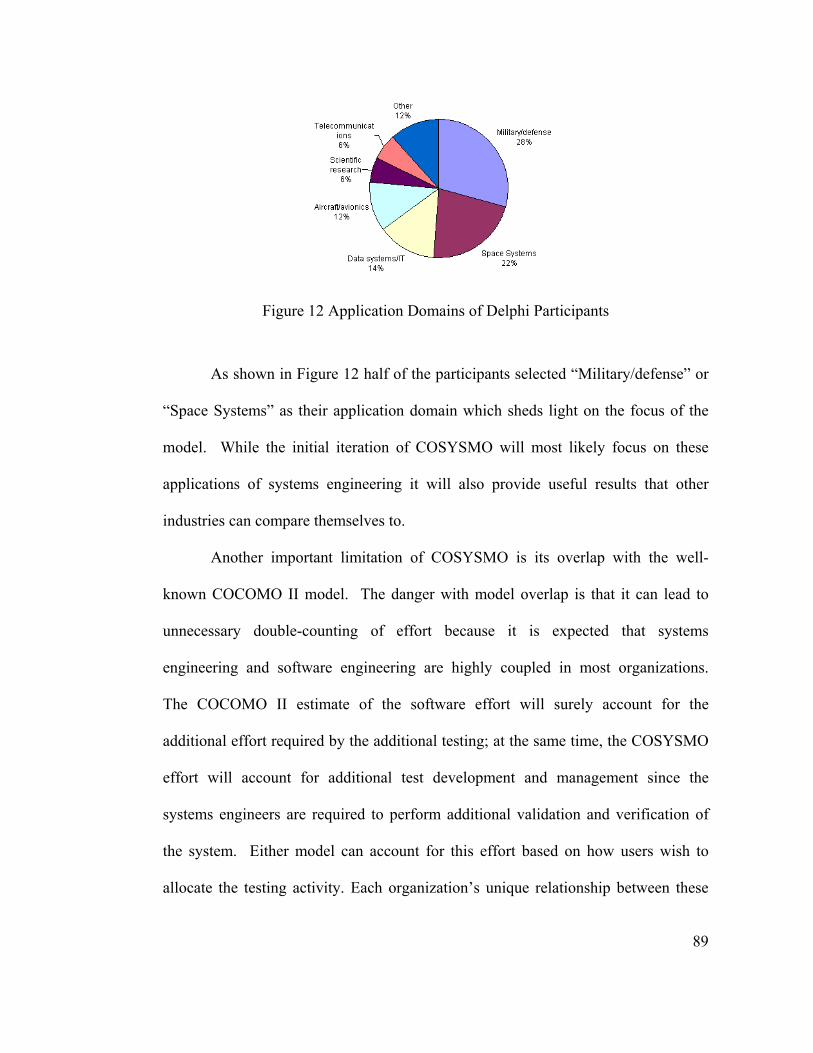
89
Figure 12 Application Domains of Delphi Participants
As shown in Figure 12 half of the participants selected “Military/defense” or
“Space Systems” as their application domain which sheds light on the focus of the
model. While the initial iteration of COSYSMO will most likely focus on these
applications of systems engineering it will also provide useful results that other
industries can compare themselves to.
Another important limitation of COSYSMO is its overlap with the well-
known COCOMO II model. The danger with model overlap is that it can lead to
unnecessary double-counting of effort because it is expected that systems
engineering and software engineering are highly coupled in most organizations.
The COCOMO II estimate of the software effort will surely account for the
additional effort required by the additional testing; at the same time, the COSYSMO
effort will account for additional test development and management since the
systems engineers are required to perform additional validation and verification of
the system. Either model can account for this effort based on how users wish to
allocate the testing activity. Each organization’s unique relationship between these
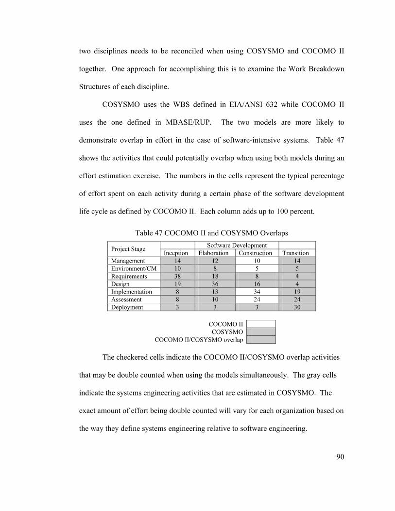
90
two disciplines needs to be reconciled when using COSYSMO and COCOMO II
together. One approach for accomplishing this is to examine the Work Breakdown
Structures of each discipline.
COSYSMO uses the WBS defined in EIA/ANSI 632 while COCOMO II
uses the one defined in MBASE/RUP. The two models are more likely to
demonstrate overlap in effort in the case of software-intensive systems. Table 47
shows the activities that could potentially overlap when using both models during an
effort estimation exercise. The numbers in the cells represent the typical percentage
of effort spent on each activity during a certain phase of the software development
life cycle as defined by COCOMO II. Each column adds up to 100 percent.
Table 47 COCOMO II and COSYSMO Overlaps Software Development Project Stage Inception Elaboration Construction Transition
Management 14 12 10 14 Environment/CM 10 8 5 5 Requirements 38 18 8 4 Design 19 36 16 4 Implementation 8 13 34 19 Assessment 8 10 24 24 Deployment 3 3 3 30
COCOMO II COSYSMO
COCOMO II/COSYSMO overlap The checkered cells indicate the COCOMO II/COSYSMO overlap activities
that may be double counted when using the models simultaneously. The gray cells
indicate the systems engineering activities that are estimated in COSYSMO. The
exact amount of effort being double counted will vary for each organization based on
the way they define systems engineering relative to software engineering.
91
5. Results and Next Steps
5.1. Delphi Results
A Delphi exercise was conducted to reach group consensus and validate
initial findings. The Wideband Delphi technique has been identified as being a
powerful tool for achieving group consensus on decisions involving unquantifiable
criteria (Boehm 1981). It was used it to circulate the initial findings and reach
consensus on the parametric ratings provided by experts. The cumulative experience
of the experts in the second round includes over 200 years of cost estimation and 600
years of systems engineering. Part of the Wideband Delphi technique involves face-
to-face meetings to review the results of the previous round and discuss any possible
changes. Eleven COSYSMO Wideband Delphi meetings took place between March
2002 and March 2004.
Part of the Delphi process involved multiple distributions of the surveys to
arrive at the values that experts could converge on. The purpose of the survey was to
(1) reach consensus from a sample of systems engineering experts, (2) determine the
distribution of effort across effort categories, (3) validate the drivers of systems
engineering size, (4) identify the cost drivers which have the most influence on effort,
and (5) help the refinement of the scope of the model elements.
Each size driver reflects the range of impact and variation assigned by the
experts during the refinement exercises. The group of size drivers includes a
volatility factor that accounts for the amount of change that is involved in the four
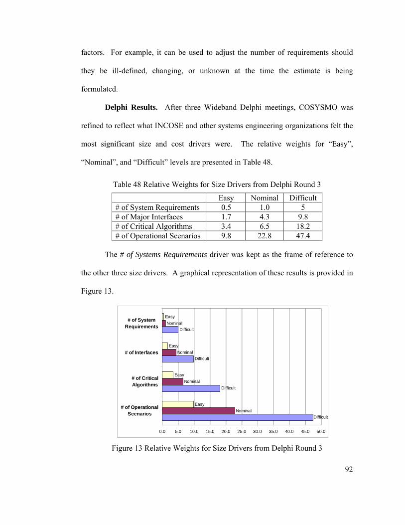
92
factors. For example, it can be used to adjust the number of requirements should
they be ill-defined, changing, or unknown at the time the estimate is being
formulated.
Delphi Results. After three Wideband Delphi meetings, COSYSMO was
refined to reflect what INCOSE and other systems engineering organizations felt the
most significant size and cost drivers were. The relative weights for “Easy”,
“Nominal”, and “Difficult” levels are presented in Table 48.
Table 48 Relative Weights for Size Drivers from Delphi Round 3
Easy Nominal Difficult # of System Requirements 0.5 1.0 5 # of Major Interfaces 1.7 4.3 9.8 # of Critical Algorithms 3.4 6.5 18.2 # of Operational Scenarios 9.8 22.8 47.4
The # of Systems Requirements driver was kept as the frame of reference to
the other three size drivers. A graphical representation of these results is provided in
Figure 13.
Difficult
Difficult
Difficult
Difficult
Nominal
Nominal
Nominal
Nominal
Easy
Easy
Easy
Easy
0.0 5.0 10.0 15.0 20.0 25.0 30.0 35.0 40.0 45.0 50.0
# of OperationalScenarios
# of CriticalAlgorithms
# of Interfaces
# of SystemRequirements
Figure 13 Relative Weights for Size Drivers from Delphi Round 3
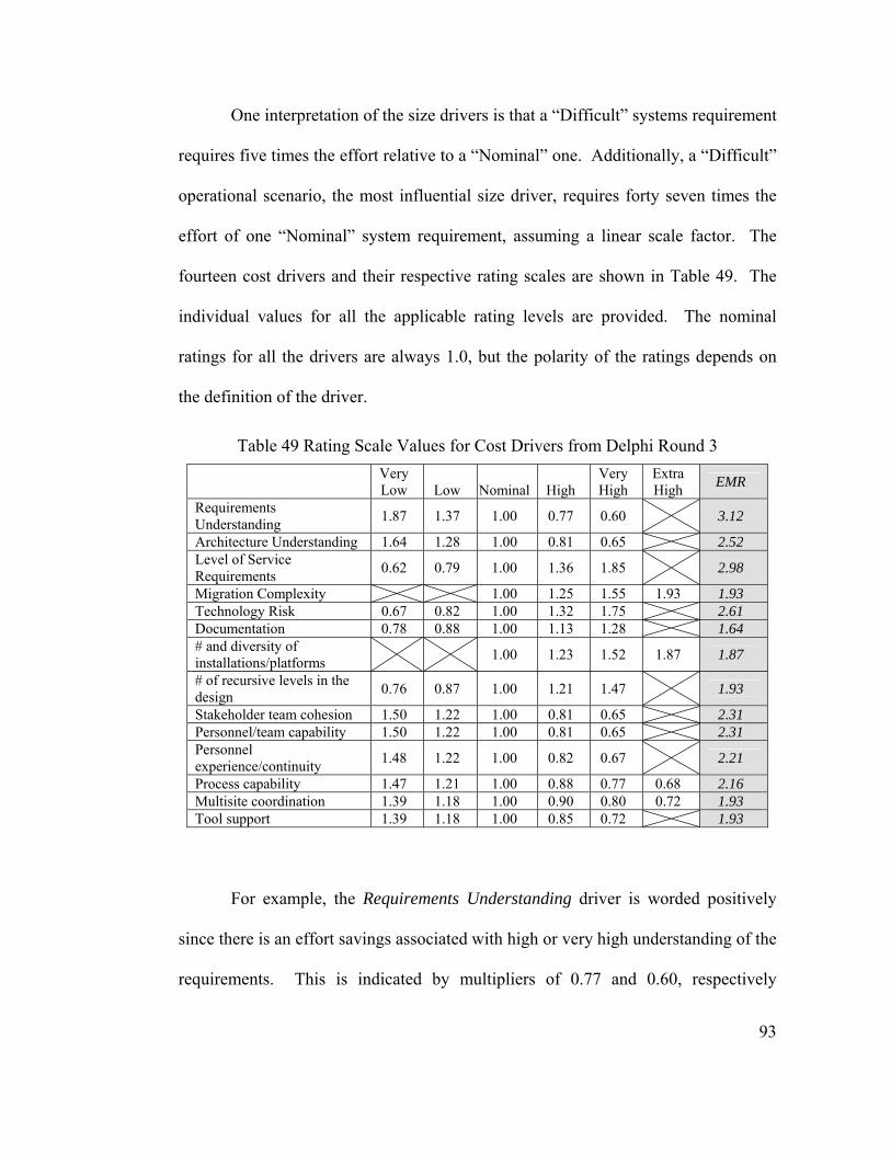
93
One interpretation of the size drivers is that a “Difficult” systems requirement
requires five times the effort relative to a “Nominal” one. Additionally, a “Difficult”
operational scenario, the most influential size driver, requires forty seven times the
effort of one “Nominal” system requirement, assuming a linear scale factor. The
fourteen cost drivers and their respective rating scales are shown in Table 49. The
individual values for all the applicable rating levels are provided. The nominal
ratings for all the drivers are always 1.0, but the polarity of the ratings depends on
the definition of the driver.
Table 49 Rating Scale Values for Cost Drivers from Delphi Round 3 Very
Low Low Nominal High Very High
Extra High EMR
Requirements Understanding 1.87 1.37 1.00 0.77 0.60 3.12
Architecture Understanding 1.64 1.28 1.00 0.81 0.65 2.52 Level of Service Requirements 0.62 0.79 1.00 1.36 1.85 2.98
Migration Complexity 1.00 1.25 1.55 1.93 1.93 Technology Risk 0.67 0.82 1.00 1.32 1.75 2.61 Documentation 0.78 0.88 1.00 1.13 1.28 1.64 # and diversity of installations/platforms 1.00 1.23 1.52 1.87 1.87
# of recursive levels in the design 0.76 0.87 1.00 1.21 1.47 1.93
Stakeholder team cohesion 1.50 1.22 1.00 0.81 0.65 2.31 Personnel/team capability 1.50 1.22 1.00 0.81 0.65 2.31 Personnel experience/continuity 1.48 1.22 1.00 0.82 0.67 2.21
Process capability 1.47 1.21 1.00 0.88 0.77 0.68 2.16 Multisite coordination 1.39 1.18 1.00 0.90 0.80 0.72 1.93 Tool support 1.39 1.18 1.00 0.85 0.72 1.93
For example, the Requirements Understanding driver is worded positively
since there is an effort savings associated with high or very high understanding of the
requirements. This is indicated by multipliers of 0.77 and 0.60, respectively
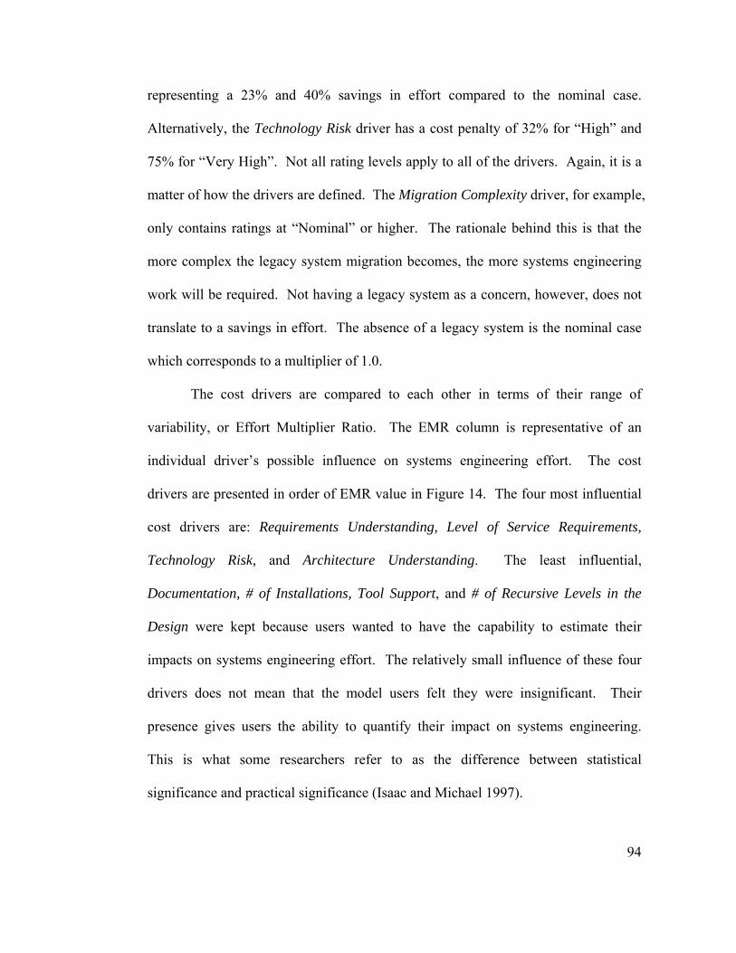
94
representing a 23% and 40% savings in effort compared to the nominal case.
Alternatively, the Technology Risk driver has a cost penalty of 32% for “High” and
75% for “Very High”. Not all rating levels apply to all of the drivers. Again, it is a
matter of how the drivers are defined. The Migration Complexity driver, for example,
only contains ratings at “Nominal” or higher. The rationale behind this is that the
more complex the legacy system migration becomes, the more systems engineering
work will be required. Not having a legacy system as a concern, however, does not
translate to a savings in effort. The absence of a legacy system is the nominal case
which corresponds to a multiplier of 1.0.
The cost drivers are compared to each other in terms of their range of
variability, or Effort Multiplier Ratio. The EMR column is representative of an
individual driver’s possible influence on systems engineering effort. The cost
drivers are presented in order of EMR value in Figure 14. The four most influential
cost drivers are: Requirements Understanding, Level of Service Requirements,
Technology Risk, and Architecture Understanding. The least influential,
Documentation, # of Installations, Tool Support, and # of Recursive Levels in the
Design were kept because users wanted to have the capability to estimate their
impacts on systems engineering effort. The relatively small influence of these four
drivers does not mean that the model users felt they were insignificant. Their
presence gives users the ability to quantify their impact on systems engineering.
This is what some researchers refer to as the difference between statistical
significance and practical significance (Isaac and Michael 1997).
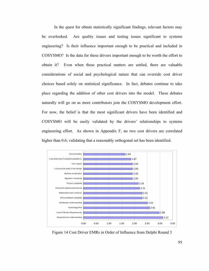
95
In the quest for obtain statistically significant findings, relevant factors may
be overlooked. Are quality issues and testing issues significant to systems
engineering? Is their influence important enough to be practical and included in
COSYSMO? Is the data for these drivers important enough to be worth the effort to
obtain it? Even when these practical matters are settled, there are valuable
considerations of social and psychological nature that can override cost driver
choices based solely on statistical significance. In fact, debates continue to take
place regarding the addition of other cost drivers into the model. These debates
naturally will go on as more contributors join the COSYSMO development effort.
For now, the belief is that the most significant drivers have been identified and
COSYSMO will be easily validated by the drivers’ relationships to systems
engineering effort. As shown in Appendix F, no two cost drivers are correlated
higher than 0.6; validating that a reasonably orthogonal set has been identified.
3.12
2.98
2.61
2.52
2.31
2.31
2.21
2.16
1.93
1.93
1.93
1.93
1.87
1.64
0.00 0.50 1.00 1.50 2.00 2.50 3.00 3.50
Requirements Understanding
Level of Service Requirements
Technology Risk
Architecture Understanding
Personnel/team capability
Stakeholder team cohesion
Personnel experience/continuity
Process capability
Migration Complexity
Multisite coordination
# of recursive levels in the design
Tool support
# and diversity of installations/platforms
Documentation
Figure 14 Cost Driver EMRs in Order of Influence from Delphi Round 3
96
5.2. Model Verification
Much energy has been spent on defining the inputs, outputs, counting rules,
definitions, and level of detail required for this model. The adage “A problem well
defined is a problem half solved” reiterates the importance of clear definitions and
model scope. In a general sense, this model has been developed in the same way as
deliverable and complex systems are, following an iterative systems engineering
approach.
The preceding chapters provided a description of the problem and an
approach. The next logical step is to shift the focus to model verification. The
process of model verification is twofold: first, a series of statistical tests are
performed. Second, feedback is obtained from end users to determine the impact of
the model. Specifically, step 5 of the model development methodology was
performed as described in (Baik, Boehm et al. 2002) using the procedure outlined in
(Chulani, Boehm et al. 1999) on the COSYSMO datapoints. This section provides
only the steps that were performed to analyze the data, not the data itself since the
source data provided by organizations is protected for reasons of industrial security.
Once data is obtained and a regression model is defined, a number of useful
diagnostics tests are helpful in validating the regression model (Snee 1977). These
include:
• Comparison of model predictors and coefficients with physical theory
• Data splitting to obtain an independent measure of the model prediction
accuracy
• Outlier/residual analysis
97
The form of the model follows the Ordinary Least Squared (OLS) criterion
because it seeks to find a simple linear regression mean function to represent the
relationship between the 18 systems engineering drivers, the independent variables,
and systems engineering effort, the dependent variable. The OLS approach has four
inherent assumptions (Griffiths, Hill et al. 1993): (1) there is a lot of data available,
(2) no outliers exist, (3) predictor variables are not correlated, and (4) predictors are
either all continuous or all discrete. In an ideal case all of these assumptions would
be true, but in reality it is difficult to find a dataset with one or more of these
characteristics. Steps have been taken to meet these assumptions as much as
possible without interfering with the systems being studied. The first assumption
was addressed by collecting data from 42 projects and 70 experts. The second
assumption was not realistic because some projects were indeed outliers and had to
be removed from the dataset due to the fact that they addressed systems engineering
size differently than other programs. The third assumption was reasonably addressed
which can be seen in Appendix F. The fourth assumption was met by making all
predictors continuous.
5.2.1. Statistical Tests
COSYSMO can be characterized by a multiple regression model where the
response is Person Months (PM) and the predictors are the 18 drivers that have an
influence on systems engineering effort. This linear function is estimated from the
data using the ordinary least squares (OLS) approach as defined by (Cook and
Weisberg 1999). The multiple regression model can be written in the form:
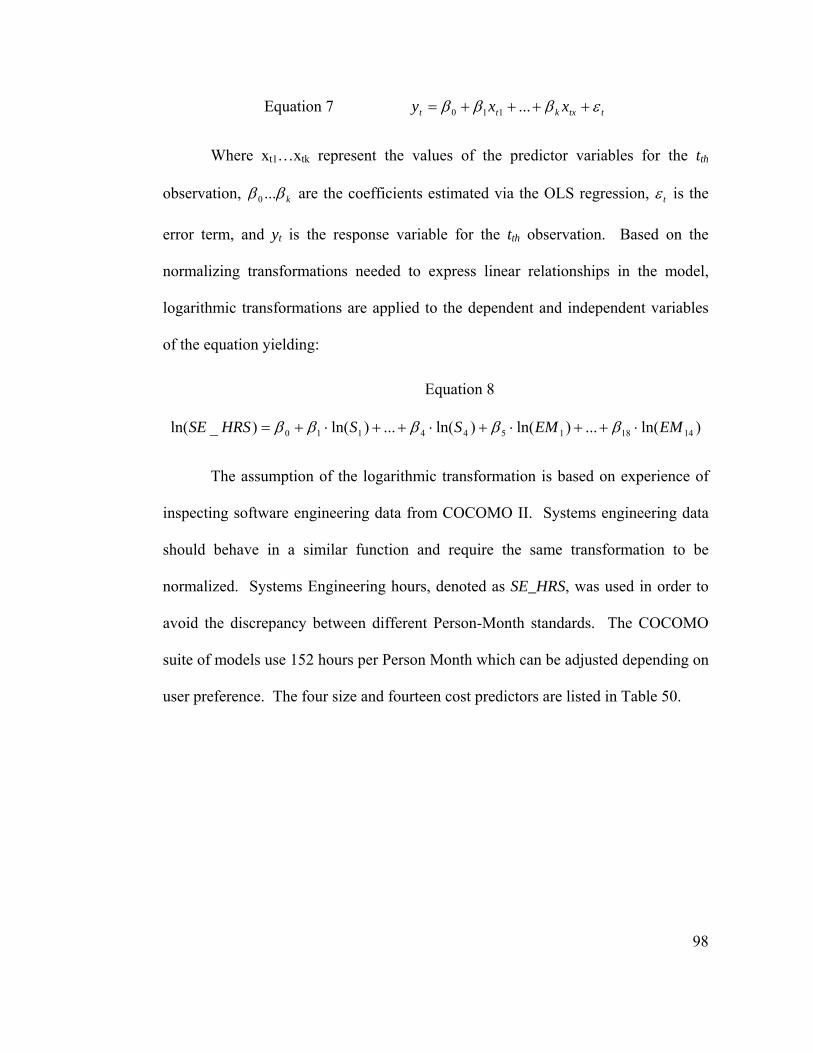
98
Equation 7 ttxktt xxy εβββ ++++= ...110
Where xt1…xtk represent the values of the predictor variables for the tth
observation, kββ ...0 are the coefficients estimated via the OLS regression, tε is the
error term, and yt is the response variable for the tth observation. Based on the
normalizing transformations needed to express linear relationships in the model,
logarithmic transformations are applied to the dependent and independent variables
of the equation yielding:
Equation 8
)ln(...)ln()ln(...)ln()_ln( 14181544110 EMEMSSHRSSE ⋅++⋅+⋅++⋅+= βββββ
The assumption of the logarithmic transformation is based on experience of
inspecting software engineering data from COCOMO II. Systems engineering data
should behave in a similar function and require the same transformation to be
normalized. Systems Engineering hours, denoted as SE_HRS, was used in order to
avoid the discrepancy between different Person-Month standards. The COCOMO
suite of models use 152 hours per Person Month which can be adjusted depending on
user preference. The four size and fourteen cost predictors are listed in Table 50.
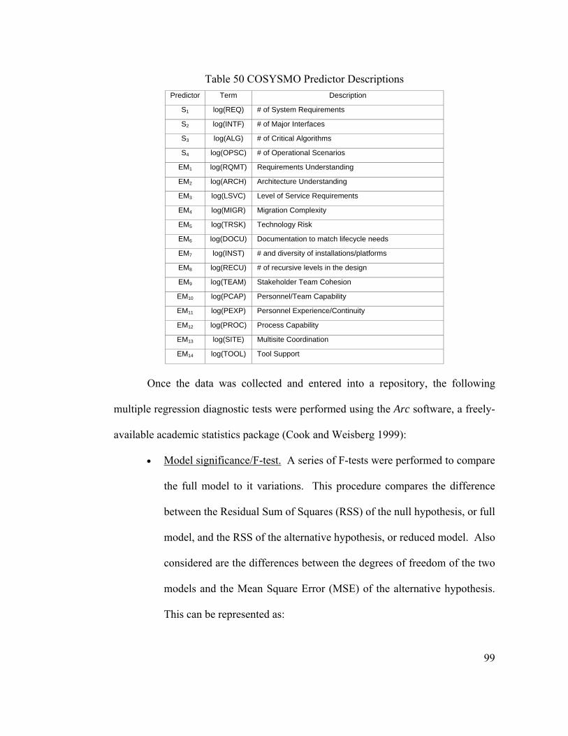
99
Table 50 COSYSMO Predictor Descriptions Predictor Term Description
S1 log(REQ) # of System Requirements
S2 log(INTF) # of Major Interfaces
S3 log(ALG) # of Critical Algorithms
S4 log(OPSC) # of Operational Scenarios
EM1 log(RQMT) Requirements Understanding
EM2 log(ARCH) Architecture Understanding
EM3 log(LSVC) Level of Service Requirements
EM4 log(MIGR) Migration Complexity
EM5 log(TRSK) Technology Risk
EM6 log(DOCU) Documentation to match lifecycle needs
EM7 log(INST) # and diversity of installations/platforms
EM8 log(RECU) # of recursive levels in the design
EM9 log(TEAM) Stakeholder Team Cohesion
EM10 log(PCAP) Personnel/Team Capability
EM11 log(PEXP) Personnel Experience/Continuity
EM12 log(PROC) Process Capability
EM13 log(SITE) Multisite Coordination
EM14 log(TOOL) Tool Support
Once the data was collected and entered into a repository, the following
multiple regression diagnostic tests were performed using the Arc software, a freely-
available academic statistics package (Cook and Weisberg 1999):
• Model significance/F-test. A series of F-tests were performed to compare
the full model to it variations. This procedure compares the difference
between the Residual Sum of Squares (RSS) of the null hypothesis, or full
model, and the RSS of the alternative hypothesis, or reduced model. Also
considered are the differences between the degrees of freedom of the two
models and the Mean Square Error (MSE) of the alternative hypothesis.
This can be represented as:
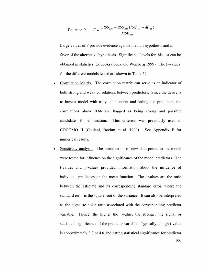
100
Equation 9 AH
AHNHAHNH
MSEdfdfRSSRSS
F)/()( −−
=
Large values of F provide evidence against the null hypothesis and in
favor of the alternative hypothesis. Significance levels for this test can be
obtained in statistics textbooks (Cook and Weisberg 1999). The F-values
for the different models tested are shown in Table 52.
• Correlation Matrix. The correlation matrix can serve as an indicator of
both strong and weak correlations between predictors. Since the desire is
to have a model with truly independent and orthogonal predictors, the
correlations above 0.66 are flagged as being strong and possible
candidates for elimination. This criterion was previously used in
COCOMO II (Chulani, Boehm et al. 1999). See Appendix F for
numerical results.
• Sensitivity analysis. The introduction of new data points to the model
were tested for influence on the significance of the model predictors. The
t-values and p-values provided information about the influence of
individual predictors on the mean function. The t-values are the ratio
between the estimate and its corresponding standard error, where the
standard error is the square root of the variance. It can also be interpreted
as the signal-to-noise ratio associated with the corresponding predictor
variable. Hence, the higher the t-value, the stronger the signal or
statistical significance of the predictor variable. Typically, a high t-value
is approximately 3.0 or 4.0, indicating statistical significance for predictor
101
variables. The p-values are an indication of evidence that the probability
of observing a value of the statistic is high or low. Values less then 0.1
are an indication of strong predictive influence on the mean function.
The t-values and p-values for the final model are shown in Appendix H.
• Stepwise Regression. Two algorithms widely available in most statistics
packages, and in this case implemented in Arc, are backward elimination
and forward elimination. These are useful in evaluating submodels by
sequentially adding or removing predictor terms and comparing the
results. Stepwise regression algorithms do not guarantee finding optimal
submodels, although the results obtained in this approach are useful in
determining candidates for elimination. This approach was previously
used in COCOMO II (Baik 2000) and for this data set helped arrive at the
reduced form of the model. Forward selection was a better indicator of
the best arrangement of predictors for COSYSMO because of the
particular behavior of the data set and small number of degrees of
freedom.
5.2.2. Model Parsimony
As stated earlier, one of the key objectives for COSYSMO is to avoid the use
of highly redundant parameters as well as factors which make no appreciable
contribution to the results. In order to achieve this, four variations of the full model
were tested to arrive at the final model that met all of the accuracy, parsimony,
constructiveness, and simplicity objectives previously defined.
102
Full model. The complete set of parameters described in sections 3.2 and 3.3
serve as the baseline model. They are listed again in Table 50 in logarithmic scale.
Equation 8 can be rewritten as:
Equation 10
log[SE_HRS] = log[REQ] + log[INTF] + log[ALG] + log[OPSC] + log[RQMT] + log[ARCH] + …+ log[TOOL]
The advantage of starting with a baseline model that contains all of the model
parameters is that tests for pair wise orthogonality can be performed. The results of
this analysis, found in Appendix F, show that no two cost drivers are correlated more
than 0.66, indicating that they represent a parsimonious set. Some of the four size
drivers are correlated as high as 0.64 which was expected since system requirements
are often related to interfaces, algorithms, and operational scenarios.
Reduced model. To address the issue of correlated size drivers and reduce
the number of predictors in the model, the four size drivers were combined into a
single predictor called Size. Equation 10 can be written as:
Equation 11
log[SE_HRS] = log[SIZE] + log[RQMT] + log[ARCH] + … + log[TOOL]
It was found that the reduced model containing the Size parameter had a
higher accuracy than the full model. In other words, the combination of the size
drivers had a higher explanatory power together rather than individually. Combining
the four size driver into one parameter also increased the degrees of freedom.
Adjusted model. The systems engineering hours for the projects reported by
participants were not provided uniformly. Only 13 of the 42 projects provided effort
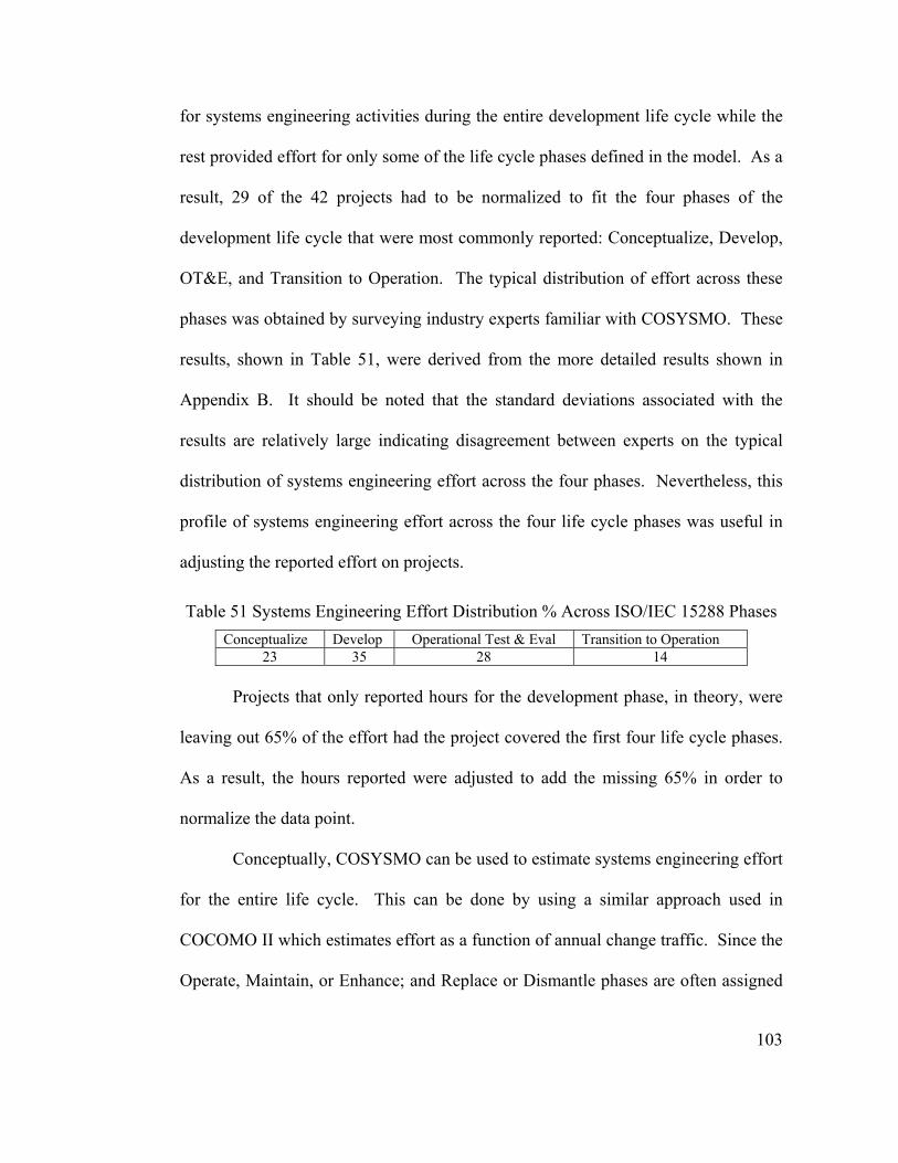
103
for systems engineering activities during the entire development life cycle while the
rest provided effort for only some of the life cycle phases defined in the model. As a
result, 29 of the 42 projects had to be normalized to fit the four phases of the
development life cycle that were most commonly reported: Conceptualize, Develop,
OT&E, and Transition to Operation. The typical distribution of effort across these
phases was obtained by surveying industry experts familiar with COSYSMO. These
results, shown in Table 51, were derived from the more detailed results shown in
Appendix B. It should be noted that the standard deviations associated with the
results are relatively large indicating disagreement between experts on the typical
distribution of systems engineering effort across the four phases. Nevertheless, this
profile of systems engineering effort across the four life cycle phases was useful in
adjusting the reported effort on projects.
Table 51 Systems Engineering Effort Distribution % Across ISO/IEC 15288 Phases Conceptualize Develop Operational Test & Eval Transition to Operation
23 35 28 14 Projects that only reported hours for the development phase, in theory, were
leaving out 65% of the effort had the project covered the first four life cycle phases.
As a result, the hours reported were adjusted to add the missing 65% in order to
normalize the data point.
Conceptually, COSYSMO can be used to estimate systems engineering effort
for the entire life cycle. This can be done by using a similar approach used in
COCOMO II which estimates effort as a function of annual change traffic. Since the
Operate, Maintain, or Enhance; and Replace or Dismantle phases are often assigned
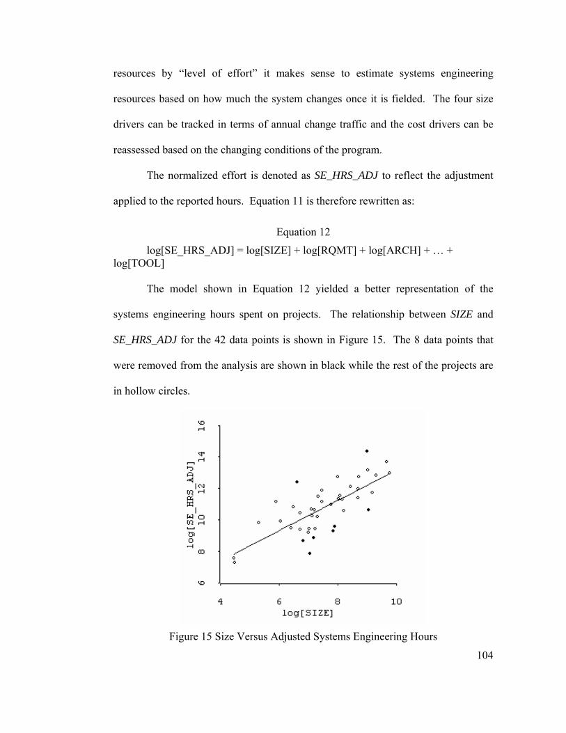
104
resources by “level of effort” it makes sense to estimate systems engineering
resources based on how much the system changes once it is fielded. The four size
drivers can be tracked in terms of annual change traffic and the cost drivers can be
reassessed based on the changing conditions of the program.
The normalized effort is denoted as SE_HRS_ADJ to reflect the adjustment
applied to the reported hours. Equation 11 is therefore rewritten as:
Equation 12
log[SE_HRS_ADJ] = log[SIZE] + log[RQMT] + log[ARCH] + … + log[TOOL]
The model shown in Equation 12 yielded a better representation of the
systems engineering hours spent on projects. The relationship between SIZE and
SE_HRS_ADJ for the 42 data points is shown in Figure 15. The 8 data points that
were removed from the analysis are shown in black while the rest of the projects are
in hollow circles.
Figure 15 Size Versus Adjusted Systems Engineering Hours
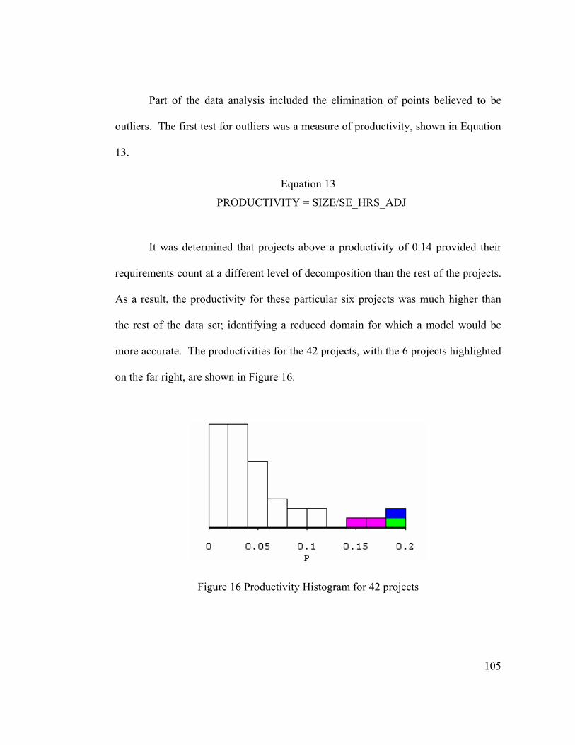
105
Part of the data analysis included the elimination of points believed to be
outliers. The first test for outliers was a measure of productivity, shown in Equation
13.
Equation 13
PRODUCTIVITY = SIZE/SE_HRS_ADJ
It was determined that projects above a productivity of 0.14 provided their
requirements count at a different level of decomposition than the rest of the projects.
As a result, the productivity for these particular six projects was much higher than
the rest of the data set; identifying a reduced domain for which a model would be
more accurate. The productivities for the 42 projects, with the 6 projects highlighted
on the far right, are shown in Figure 16.
Figure 16 Productivity Histogram for 42 projects
106
In addition to the 6 projects eliminated due to extremely high productivity, 2
projects were also removed from the calibration domain due to a high degree of
adjusted effort (more than 30%) across the systems engineering life cycle.
Final Model. With a smaller number of data points, a smaller number of
aggregated parameters was considered. The cost drivers were clustered into groups
in section 3.3 based on common themes. These five groups were determined to be
logical groupings of cost drivers that addressed similar issues dealing with systems
engineering. This resulted in the model shown in Equation 14.
Equation 14
log[SE_HRS_ADJ] = log[SIZE] + log[UNDERSTANDING] + log[COMPLEXITY] + log[OPERATIONS] + log[PEOPLE] + log[ENVIRONMENT] Where UNDERSTANDING = REQU * ARCH * TEAM * PEXP COMPLEXITY = LSVC * TRSK * RECU * DOCU OPERATIONS = INST * MIGR PEOPLE = PCAP * PROC ENVIRONMENT = SITE * TOOL The model in Equation 14 provided additional degrees of freedom and a
higher F-value. However, not all six predictors met the p-value criterion of 0.1. See
regression results for this model in Appendix H. Nevertheless, this model was used
as the final calibrated version because it contained all of the parameters in the model
in aggregated form.
Reduced model. A reduced form of the model was developed which
includes predictors whose p-values were less than 0.1. These are shown in Equation
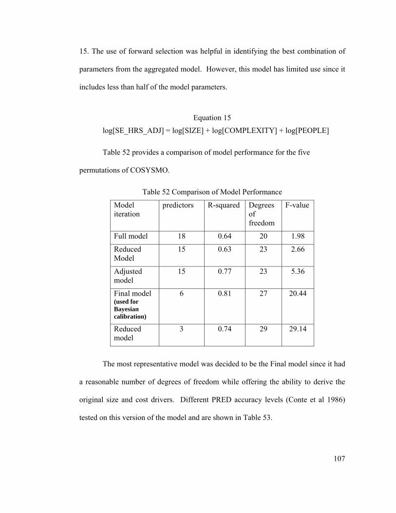
107
15. The use of forward selection was helpful in identifying the best combination of
parameters from the aggregated model. However, this model has limited use since it
includes less than half of the model parameters.
Equation 15
log[SE_HRS_ADJ] = log[SIZE] + log[COMPLEXITY] + log[PEOPLE]
Table 52 provides a comparison of model performance for the five
permutations of COSYSMO.
Table 52 Comparison of Model Performance
Model iteration
predictors R-squared Degrees of freedom
F-value
Full model 18 0.64 20 1.98
Reduced Model
15 0.63 23 2.66
Adjusted model
15 0.77 23 5.36
Final model (used for Bayesian calibration)
6 0.81 27 20.44
Reduced model
3 0.74 29 29.14
The most representative model was decided to be the Final model since it had
a reasonable number of degrees of freedom while offering the ability to derive the
original size and cost drivers. Different PRED accuracy levels (Conte et al 1986)
tested on this version of the model and are shown in Table 53.
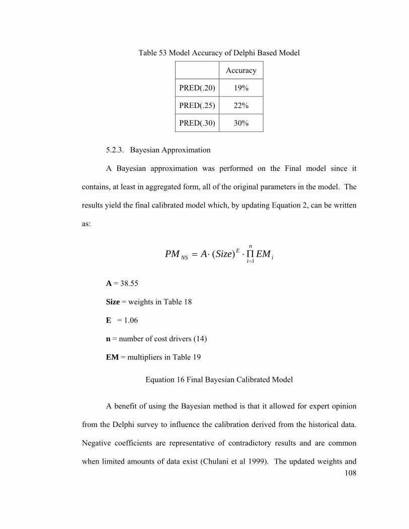
108
Table 53 Model Accuracy of Delphi Based Model
Accuracy
PRED(.20) 19%
PRED(.25) 22%
PRED(.30) 30%
5.2.3. Bayesian Approximation
A Bayesian approximation was performed on the Final model since it
contains, at least in aggregated form, all of the original parameters in the model. The
results yield the final calibrated model which, by updating Equation 2, can be written
as:
i
n
i
ENS EMSizeAPM
1)(
=Π⋅⋅=
A = 38.55
Size = weights in Table 18
E = 1.06
n = number of cost drivers (14)
EM = multipliers in Table 19
Equation 16 Final Bayesian Calibrated Model
A benefit of using the Bayesian method is that it allowed for expert opinion
from the Delphi survey to influence the calibration derived from the historical data.
Negative coefficients are representative of contradictory results and are common
when limited amounts of data exist (Chulani et al 1999). The updated weights and
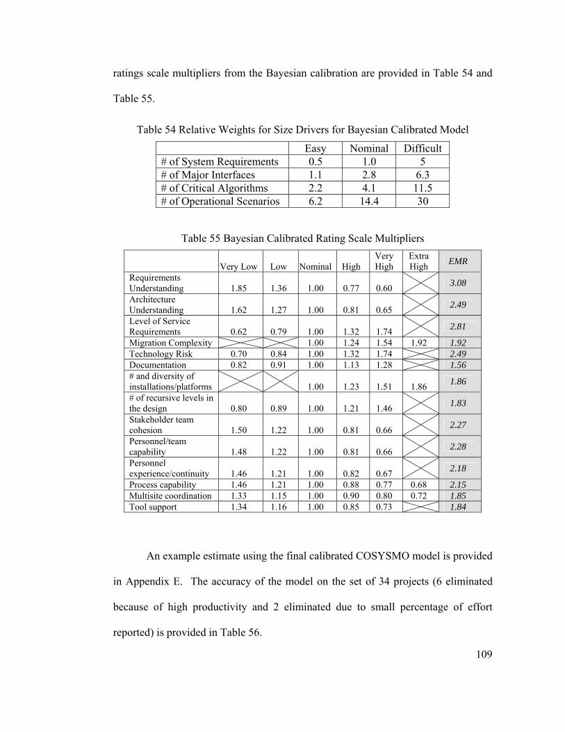
109
ratings scale multipliers from the Bayesian calibration are provided in Table 54 and
Table 55.
Table 54 Relative Weights for Size Drivers for Bayesian Calibrated Model
Easy Nominal Difficult # of System Requirements 0.5 1.0 5 # of Major Interfaces 1.1 2.8 6.3 # of Critical Algorithms 2.2 4.1 11.5 # of Operational Scenarios 6.2 14.4 30
Table 55 Bayesian Calibrated Rating Scale Multipliers
Very Low Low Nominal High Very High
Extra High EMR
Requirements Understanding 1.85 1.36 1.00 0.77 0.60 3.08
Architecture Understanding 1.62 1.27 1.00 0.81 0.65 2.49
Level of Service Requirements 0.62 0.79 1.00 1.32 1.74 2.81
Migration Complexity 1.00 1.24 1.54 1.92 1.92 Technology Risk 0.70 0.84 1.00 1.32 1.74 2.49 Documentation 0.82 0.91 1.00 1.13 1.28 1.56 # and diversity of installations/platforms 1.00 1.23 1.51 1.86 1.86
# of recursive levels in the design 0.80 0.89 1.00 1.21 1.46 1.83
Stakeholder team cohesion 1.50 1.22 1.00 0.81 0.66 2.27
Personnel/team capability 1.48 1.22 1.00 0.81 0.66 2.28
Personnel experience/continuity 1.46 1.21 1.00 0.82 0.67 2.18
Process capability 1.46 1.21 1.00 0.88 0.77 0.68 2.15 Multisite coordination 1.33 1.15 1.00 0.90 0.80 0.72 1.85 Tool support 1.34 1.16 1.00 0.85 0.73 1.84
An example estimate using the final calibrated COSYSMO model is provided
in Appendix E. The accuracy of the model on the set of 34 projects (6 eliminated
because of high productivity and 2 eliminated due to small percentage of effort
reported) is provided in Table 56.
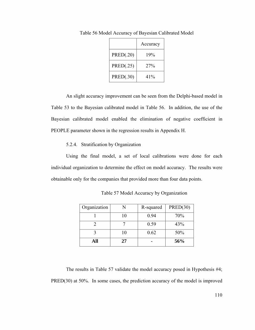
110
Table 56 Model Accuracy of Bayesian Calibrated Model
Accuracy
PRED(.20) 19%
PRED(.25) 27%
PRED(.30) 41%
An slight accuracy improvement can be seen from the Delphi-based model in
Table 53 to the Bayesian calibrated model in Table 56. In addition, the use of the
Bayesian calibrated model enabled the elimination of negative coefficient in
PEOPLE parameter shown in the regression results in Appendix H.
5.2.4. Stratification by Organization
Using the final model, a set of local calibrations were done for each
individual organization to determine the effect on model accuracy. The results were
obtainable only for the companies that provided more than four data points.
Table 57 Model Accuracy by Organization
Organization N R-squared PRED(30)
1 10 0.94 70%
2 7 0.59 43%
3 10 0.62 50%
All 27 - 56%
The results in Table 57 validate the model accuracy posed in Hypothesis #4;
PRED(30) at 50%. In some cases, the prediction accuracy of the model is improved
111
even further when the organization’s disciplined data collection has uniform
counting rules that can ensure consistency across programs. Regardless of the results
provided by the statistical validation, limitations of the model should be considered
when the prediction accuracy of the model is determined. Limitations were provided
in previous sections as were their implications on model validity.
In addition to the rigorous quantitative analysis of the model, a qualitative
analysis was performed to determine the impact of the model on each organization
that provided data. COSYSMO supporters were enthusiastic about the model’s
influence in the way their organizations thought about systems engineering cost. Out
of 8 participants queried, 7 of them responded that COSYSMO greatly improved
their ability to reason about systems engineering cost. Example testimonials include:
• Model helps answer the call for improvement on systems engineering
revitalization and ensuring adequate SE resources identified in the Young
Panel report for DoD Space Systems
• The size and effort drivers will allow the user of the model to best describe
the project and to perform sensitivity analysis to try to optimize the SE
application and team aspects of the project
• COSYSMO answers the ‘CMMI mail’ regarding a key requirement for
Maturity Level 2: Costing by Attributes ---- specifically, counts of System
Requirements, System Interfaces, Critical Algorithms, and Operational
Scenarios as scaled by the environmental (team and application) cost drivers.
112
5.3. Conclusion
A new type of systems engineering cost model was presented and validated
through industry data. An objectively reduced subset of 42 industry projects from 6
companies was used to calibrate the model in reduced form which produced a
PRED(30) accuracy of 50%. Together with counting rules and driver definitions, the
model provides a way for systems engineers to reason about their cost decisions and
presents a new vehicle for managers to approach systems engineering strategy via
size and cost metrics.
Restatement of hypotheses. The five hypotheses stated in Section 1.3 were
tested to determine their validity.
H#1: A combination of the four elements of functional size in COSYSMO
contributes significantly to the accurate estimation of systems engineering
effort.
The criterion used was a significance level less than or equal to 0.10 which
translates to a 90% confidence level that these elements are significant. This
hypothesis was supported with the reduced form of the model.
H#2: An ensemble of COSYSMO effort multipliers contribute significantly to
the accurate estimation of systems engineering.
The same significance level of 0.10 was used to test this hypothesis which
was supported with the reduced form of the model.
H#3: The value of the COSYSMO exponent, E, which can represent
economies/diseconomies of scale is greater than 1.0.
113
For some organizations, the exponent was as low as 0.83 and as high as 1.31,
as a result this hypothesis was partially supported. The average value for E was 1.06.
H#4: There exists a subset of systems engineering projects for which it is
possible to create a parametric model that will estimate systems engineering effort at
a PRED(30) accuracy of 50%.
This hypothesis was supported with the subset of projects defined as the
projects from organizations with more than 4 solid data points with systems
engineering productivity below 0.14 size units per adjusted SE hours.
H#5: COSYSMO makes organizations think differently about Systems
Engineering cost.
This hypothesis was strongly supported. Seven out of eight responded with
resounding support within the COSYSMO pioneer community as evidenced by the
testimonials in section 5.2.4; insufficient data elsewhere.
5.3.1. Contributions to the Field of Systems Engineering
This work has a number of significant contributions to the field of systems
engineering. These contributions have implications for researchers, practitioners,
and educators.
1. Development of a parametric Systems Engineering cost model. Practitioners
will benefit from the creation of COSYSMO because it is the first cost
estimation model that provides systems engineering effort estimation. The
identification of significant size and cost drivers for systems engineering can
also serve as a risk management list for projects.
114
2. Systems Engineering Sizing. The development of counting rules for systems
engineering using non-software metrics such as lines of code or function
points is a significant contribution to the field of parametric cost modeling.
3. Operationalization of cost drivers and rating scales. The list of 14 cost
drivers, their definitions, and their Cost Estimating Relationships provide
useful teaching tools for systems engineering educators. Results show that
these cost drivers are independent of each other and are good indicators of
systems engineering complexity. A list of the cost drivers in order of
influence was also generated to help people identify the factors that have the
largest influence on cost.
4. SE as an independent discipline. Organizations such as INCOSE will benefit
from COSYSMO because it helps justify the value of systems engineering in
organizations. Researchers in the area of parametrics can also build from this
work to develop additional CERs that are independent of software or
hardware development.
5. Development of the first systems engineering focused model. COSYSMO
can also help efforts currently underway to develop frameworks and theories
related to systems engineering. One such example is the Grand Unified
Theory of Systems Engineering (GUTSE) developed by George Friedman
(Friedman 2003) which implies the future existence of a reliable cost model
but currently does not include such a model.
6. Institutional memory. The development of COSYSMO has captured over
500 person years of experience in systems engineering experience from over
115
a dozen heterogeneous organizations. This baseline model can help
researchers and educators develop case studies that can further the
understanding of systems engineering.
7. Convergence. Industry experts were orchestrated to determine Delphi
weights, driver definitions, counting rules, model form, and model scope.
Convergence on these values demonstrates industry collaboration through the
facilitation of academic researchers.
8. Evidence of diseconomy of scale. Empirical evidence verifies the hypothesis
that systems engineering effort exhibits a diseconomy of scale.
9. Systems engineering effort profile. Through expert opinion, an effort profile
was developed using the fundamental processes in ANSI/EIA 632 to define
the model scope and distribute effort estimates across activities.
In addition to the practitioners that have benefited from COSYSMO, the
following educational institutions have incorporated it into their systems engineering
syllabus: University of California San Diego, George Mason University, Defense
Acquisition University, and Southern Methodist University.
5.3.2. Areas for Future Work
The estimation of systems engineering cost is a complex but much needed
process. The acquisition community continues to demand more accurate
quantification of the SE work that is performed on hardware and software systems.
In order to realize more sophisticated methods for estimating SE effort, the models
should be based on empirical data. Rather than using rules of thumb, models should
be data-driven. Instead of having limited relevance only to standard life cycles, they
116
should be more flexible. Further work is required to make the task of managing SE
more quantitative.
This section is divided into two parts to reflect the areas for future work that
are needed in the short term and the long term. The short term areas are ones that
will need to be addressed as extensions of this dissertation work while the long term
are ones that can provide future opportunities for research in this area.
The process of developing COSYSMO has produced a number of useful Cost
Estimating Relationships (CERs) that aid in estimating systems engineering effort.
These CERs are accompanied by a set of rules that help guide the user in defining
the scope of COSYSMO and how it relates to their organization. One of the
challenges of creating a generalizable model is that it has to be flexible enough to
work in different application domains. These domains operate differently by the
nature of the customers they serve, the systems they build, and the environment in
which their systems must operate. COSYSMO constituents represent a diverse set of
users that represent an additional level of complexity because of their heterogeneous
nature. This diversity has introduced the following challenges that need to be
resolved:
1. Effects of volatility and reuse. These effects were deferred because of the
difficulty in gathering data to calibrate them. Future work should
incorporate these relevant parameters into the model.
2. Requirements counting. The different levels of requirements decomposition
that are used by organizations was previously presented. More specific
counting rules need to be developed to ensure consistency in this area.
117
3. The SEMP. Effects of the Systems Engineering Management Plan (SEMP)
is currently not included in COSYSMO, however, it plays a significant role
in the effectiveness of systems engineering organizations. For the time being,
it has been included as part of the Process Capability cost driver. Future
exploration is required to define the best rating scale that captures its
influence on systems engineering effort.
4. Drivers with multiple viewpoints. The consolidation of the model discussed
in Chapter 8 brought about an overloading of some cost drivers. This was
caused by the merging of two or more drivers into one resulting in the
introduction of multiple viewpoints for some drivers. Drivers such as
Technology Risk, Multisite Coordination, Migration Complexity, and # and
Diversity of Installations & Platforms have two or more aspects of systems
engineering embedded in their definitions. These need to be simplified or
rolled into separate cost drivers.
5. CMMI & Key Process Areas. The influence of CMMI as a cornerstone of
this model was highlighted in section 3. However, not every organization
has adopted the CMMI framework in its processes. As a result, an
alternative method for measuring the process capability of an organization
needs to be developed through the use of Key Process Areas (KPAs).
Moreover, some confusion exists in situations where multiple organizations
with different levels of maturity are operating under the same contract. This
situation is difficult to quantify from the COSYSMO standpoint and needs to
be resolved.
118
6. Technology Readiness Levels. Another difficulty in quantifying a cost
driver occurs when multiple technologies with different maturity levels and
different time horizons have an effect on the systems engineering
organization(s).
7. EIA/ANSI 632 activities. The menu of EIA/ANSI 632 activities listed in
Chapter 3 represents an industry standard which is not entirely applicable in
practice. Further investigation is needed to determine which systems
engineering activities in EIA/ANSI 632 are more likely to be performed by
organizations using COSYSMO.
8. Compatibility with other models. The MBASE framework presented
includes several other product models that are closely related to systems
engineering. Software engineering activities estimated by COCOMO and
system of system software integration activities estimated by COSOSIMO
need to be clearly delineated to ensure minimal overlap or ways to account
for their overlap with COSYSMO.
9. Need more data. The list of organizations that have contributed data
provided enough data to calibrate an initial model, but more data is needed in
order to perform more tests of significance on all the model parameters.
10. Need more commercial company involvement. The same list of
aforementioned organizations indicates a heavy bias toward aerospace and
military projects. More commercial companies’ data needs to be obtained
and incorporated into the model calibration.
119
Long Term Areas. In order for COSYSMO to be a useful tool for the
systems engineering community it must be adaptable to a situation of interest. The
initial release of the model will have an industry baseline calibration that is
representative of the CERs and driver definitions at the industry level. The model
will be much more useful to individual organizations if it is calibrated for their use.
This and other adaptations to the model are long term opportunities for future
research.
1. COSYSMO Tailoring. Customizing the model to meet the needs of
organizations is necessary to maximize the model’s predictive ability. Local
calibrations should be done and, if possible, product line calibrations for a
specific family of products and customer calibrations for particular
operational environments.
2. Additional driver definitions. Part of the customization process may involve
the development of additional cost or size drivers. This alternative should
especially be investigated by commercial companies that participated in the
initial calibration.
3. Maintenance model. The CERs for systems engineering may behave
differently in the maintenance phase of the project life cycle. This could
serve as an opportunity to develop a COSYSMO maintenance model.
4. Tool comparison matrix. The development of a tool comparison matrix
would be of value to enable the selection of the most appropriate cost
estimating tool for a particular project. Such a comparison would establish
uniform definitions and factors that would encompass the breadth of how
120
COCOMO, COSYSMO, and COSOSIMO assess systems engineering. Such
a comparison would facilitate identification of areas lacking sufficient detail
and establish understanding to appropriately quantify systems engineering.
These findings would suggest common areas of enhancement and
development for additional research.
5. Risk Analyzer. Since COSYSMO provides a single point estimate, it would
benefit from a risk analysis tool that determines the amount of risk associated
with a given estimate.
6. Additional behavioral implications. The process of effort estimation involves
unique skills and knowledge about how people work together and how
organizations interact with each other. It would be interesting to investigate
how other types of knowledge can affect the process of cost estimation.
Some possible areas of investigation are: codified knowledge, Herbert
Simon’s bounded rationality (what is in and what is out), Eric von Hippel’s
sticky information (people’s ability to remember things), Eugene Ferguson’s
idea of the mind’s eye (aesthetic knowledge), and group think.
As industry and academia collaborate to develop and validate a tool to more
accurately forecast SE resources, more opportunities for research are created. These
areas could potentially change the way cost estimation models are developed and
used.
121
References Abts, C., Boehm, B. W. and Bailey-Clark, E. (2001). COCOTS : A Software COTS-
Based System (CBS) Cost Model - Evolving Towards Maintenance Phase Modeling. Proceedings of the Twelfth Software Control and Metrics Conference, London, England.
Ahern, D. M., Clouse, A. and Turner, R. (2004). CMMI Distilled - A Practical Guide
to Integrated Process Improvement, Addison-Wesley. Albrecht, A. J., Gaffney, J., (1983), “Software function, source lines of code, and
development effort prediction: A software Science validation,” IEEE Transactions on Software Engineering, Vol. SE-9, pp. 639-648.
ANSI/EIA (1999). ANSI/EIA-632-1988 Processes for Engineering a System. ANSI/EIA (2002). EIA-731.1 Systems Engineering Capability Model. Auyang, S. Y. (2004). Engineering – An Endless Frontier. Cambridge, MA, Harvard
University Press. Babbie, E. (2004). The Practice of Social Research, Wadsworth. Baik, J. (2000). The Effect of CASE Tools on Software Development Effort.
Unpublished Dissertation, USC Computer Science Department. Baik, J., Boehm, B. W. and Steece, B. (2002). "Disaggregating and Calibrating the
CASE Tool Variable in COCOMO II." IEEE Transactions on Software Engineering Vol. 28(No. 11).
Berne, E. (1964). Games People Play: The Psychology of Human Relationships.
New York, Grove Press, Inc. Blanchard, B. S. and Fabrycky, W. J. (1998). Systems Engineering and Analysis,
Prentice Hall. Boehm, B. W. (1981). Software Engineering Economics, Prentice-Hall. Boehm, B. W. (1994). "Integrating Software Engineering and Systems Engineering."
The Journal of NCOSE Vol. 1 (No. 1): pp. 147-151. Boehm, B. W., Egyed, A. and Abts, C. (1998). Proceedings Focused Workshop #10:
Software Engineering and System Engineering, Center for Software Engineering.
122
Boehm, B. W. and Port, D. (1999). "Escaping the Software Tar Pit: Model Clashes and How to Avoid Them." ACM Software Engineering Notes.
Boehm, B. W., Abts, C., Brown, A. W., Chulani, S., Clark, B., Horowitz, E.,
Madachy, R., Reifer, D. J. and Steece, B. (2000). Software Cost Estimation With COCOMO II, Prentice Hall.
Boehm, B. W. and Hansen, W. (2001). "The Spiral Model as a Tool for Evolutionary
Acquisition." CrossTalk: pp. 4-9. Boehm, B. W., Reifer, D. J. and Valerdi, R. (2003). COSYSMO-IP: A Systems
Engineering Cost Model. 1st Annual Conference on Systems Integration, Hoboken, NJ.
Boehm, B. W., (2003) "Value-Based Software Engineering." ACM Software
Engineering Notes. Boehm, B., Valerdi, R., Lane, J., Brown, A. W., (2005) “COCOMO Suite
Methodology and Evolution,” CrossTalk - The Journal of Defense Software Engineering.
Brooks, F. P. (1995). The Mythical Man-Month: Essays on Software Engineering,
Addison-Wesley. Chulani, S., Boehm, B. W. and Steece, B. (1999). "Bayesian Analysis of Empirical
Software Engineering Cost Models." IEEE Transactions on Software Engineering: pp. 513-583.
Clark, B. K. (1997). The Effects of Software Process Maturity on Software
Development Effort. Unpublished Dissertation, USC Computer Science Department.
CMMI (2002). Capability Maturity Model Integration - CMMI-SE/SW/IPPD/SS,
V1.1. Pittsburg, PA, Carnegie Mellon - Software Engineering Institute. Conte, S. D., Dunsmore, H. E., Shen, V. Y., (1986) Software Engineering Metrics
and Models, Benjamin/Cummings Publishing Company. Cook, D. and Weisberg, S. (1999). Applied Regression Including Computing and
Graphics, John Wiley & Sons. Dalkey, N. (1969). The Delphi Method: An Experimental Study of Group Opinion,
RAND Corporation.

123
Ernstoff, M. and Vincenzini, I. (1999). Guide to Products of System Engineering. International Council on Systems Engineering, Las Vegas, NV.
Faisandier, A, Lake, J., Harmonization of Systems and Software Engineering,
INCOSE INSIGHT, Vol. 7, Issue 3., October 2004. Ferens, D. (1999). Parametric Estimating - Past, Present, and Future. 19th PRICE
European Symposium. Freud, S. (1924). A General Introduction to Psycho-Analysis. New York,
Washington Square Press, Inc. Friedman, G. (2003). ISE541 Lecture Notes. USC Industrial & Systems Engineering. GAO-03-1073 (2003). Defense Acquisitions Improvements Needed in Space
Systems Acquisition Management Policy. Griffiths, W. E., Hill, R. C. and Judge, G. G. (1993). Learning and Practicing
Econometrics, John Wiley & Sons, Inc. Honour, E. C. (2002). Toward an Understanding of the Value of Systems
Engineering. First Annual Conference on Systems Integration, Hoboken, NJ. Horowitz, B. (2004). Systems Engineering Estimation Rules of Thumb. R. Valerdi.
Charlottesville, VA: Personal communication. Humel, P. (2003). Systems Engineering Revitalization at Space and Missile Systems
Center. INCOSE Los Angeles Chapter Meeting, The Aerospace Corporation. Isaac, S. and Michael, W. B. (1997). Handbook in Research and Evaluation. San
Diego, CA, EdITS. ISO/IEC (2002). ISO/IEC 15288:2002(E) Systems Engineering - System Life Cycle
Processes. Jackson, S. (2002). ISE541 Lecture Notes. USC Industrial & Systems Engineering. Jarvenpaa, S. L., G. W. Dickson, G. W. and DeSanctis, G. (1985). "Methodological
Issues in Experimental IS Research: Experiences and Recommendations." MIS Quarterly Vol. 9(No. 2).
Kemerer, C. (1987). "An Empirical Validation of Software Cost Estimation Models."
Communications of the ACM Vol. 30(No. 5): pp. 416-429.
124
Klein, H. K. and Myers, M. D. (1999). "A Set of Principles for Conducting and Evaluating Interpretive Field Studies in Information Systems." MIS Quarterly Vol. 23 (No. 1).
MIL-STD 490-A (1985) Specification Practices. MIL-STD-499A (1969). Engineering Management. NASA (2002). Cost Estimating Handbook. Pandikow, A. and Törne, A. (2001). Integrating Modern Software Engineering and
Systems Engineering Specification Techniques. 14th International Conference on Software & Systems Engineering and their Applications.
PRICE-H (2002). Your Guide to PRICE-H: Estimating Cost and Schedule of
Hardware Development and Production. Mt. Laurel, NJ, PRICE Systems, LLC.
Rechtin, E. (1991). Systems Architecting: Creating & Building Complex Systems,
Prentice Hall. Rechtin, E. (1998). System and Software Architecture. Proceedings Focused
Workshop #10: Software Engineering and System Engineering. Sage, A. P. (1992). Systems Engineering, John Wiley & Sons, Inc. Sheard, S. (1997). The Frameworks Quagmire, A Brief Look. Proceedings for the
Seventh Annual Symposium of the International Council on Systems Engineering, Los Angeles, CA.
Shrum, S. (2000). "Choosing a CMMI Model Representation." CrossTalk. Smith, J. (2004). An Alternative to Technology Readiness Levels for Non-
Developmental Item (NDI) Software - CMU/SEI-2004-TR-013. Pittsburg, PA, Carnegie Mellon - Software Engineering Institute.
Snee, R. (1977). "Validation of Regression Models: Methods and Examples."
Technometrics Vol. 19 (No. 4). Sudman, S. and Bradburn, N. M. (1982). Asking Questions: A Practical Guide to
Questionnaire Design. San Francisco, CA, Jossey-Bass. USCM (2002). USCM8 Knowledge Management System, Tecolote Research, Inc.
125
Valerdi, R., Ernstoff, M., Mohlman, P., Reifer, D. and Stump, E. (2003). Systems Engineering Sizing in the Age of Acquisition Reform. 18th Annual Forum on COCOMO and Software Cost Modeling, Los Angeles, CA.
Valerdi, R. and Kohl, R. (2004). An Approach to Technology Risk Management. 1st
Annual MIT Engineering Systems Division Symposium, Cambridge, MA. Valerdi, R., Rieff, J. E., Roedler, G. J. and Wheaton, M. J. (2004). Lessons Learned
From Collecting Systems Engineering Data. Ground Systems Architecture Workshop, El Segundo, CA.
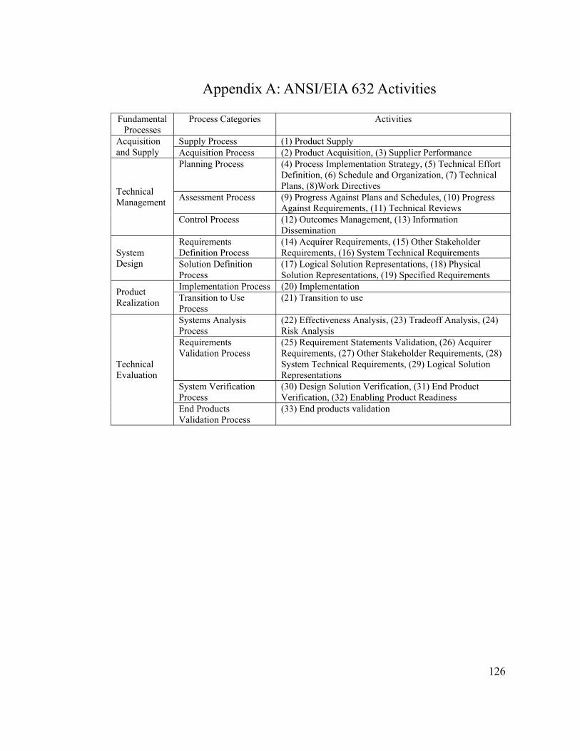
126
Appendix A: ANSI/EIA 632 Activities Fundamental
Processes Process Categories Activities
Supply Process (1) Product Supply Acquisition and Supply Acquisition Process (2) Product Acquisition, (3) Supplier Performance
Planning Process (4) Process Implementation Strategy, (5) Technical Effort Definition, (6) Schedule and Organization, (7) Technical Plans, (8)Work Directives
Assessment Process (9) Progress Against Plans and Schedules, (10) Progress Against Requirements, (11) Technical Reviews
Technical Management
Control Process (12) Outcomes Management, (13) Information Dissemination
Requirements Definition Process
(14) Acquirer Requirements, (15) Other Stakeholder Requirements, (16) System Technical Requirements System
Design Solution Definition Process
(17) Logical Solution Representations, (18) Physical Solution Representations, (19) Specified Requirements
Implementation Process (20) Implementation Product Realization Transition to Use
Process (21) Transition to use
Systems Analysis Process
(22) Effectiveness Analysis, (23) Tradeoff Analysis, (24) Risk Analysis
Requirements Validation Process
(25) Requirement Statements Validation, (26) Acquirer Requirements, (27) Other Stakeholder Requirements, (28) System Technical Requirements, (29) Logical Solution Representations
System Verification Process
(30) Design Solution Verification, (31) End Product Verification, (32) Enabling Product Readiness
Technical Evaluation
End Products Validation Process
(33) End products validation
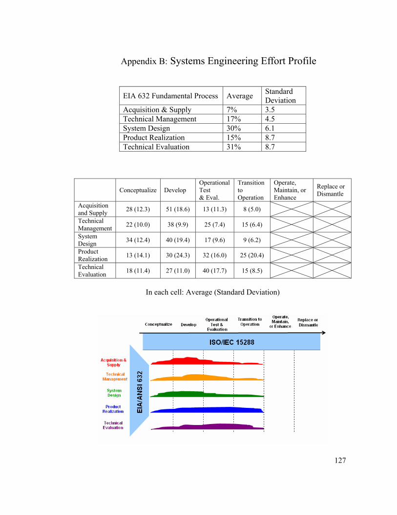
127
Appendix B: Systems Engineering Effort Profile
EIA 632 Fundamental Process Average Standard Deviation
Acquisition & Supply 7% 3.5 Technical Management 17% 4.5 System Design 30% 6.1 Product Realization 15% 8.7 Technical Evaluation 31% 8.7
Conceptualize Develop Operational Test & Eval.
Transition to Operation
Operate, Maintain, or Enhance
Replace or Dismantle
Acquisition and Supply 28 (12.3) 51 (18.6) 13 (11.3) 8 (5.0)
Technical Management 22 (10.0) 38 (9.9) 25 (7.4) 15 (6.4)
System Design 34 (12.4) 40 (19.4) 17 (9.6) 9 (6.2)
Product Realization 13 (14.1) 30 (24.3) 32 (16.0) 25 (20.4)
Technical Evaluation 18 (11.4) 27 (11.0) 40 (17.7) 15 (8.5)
In each cell: Average (Standard Deviation)

128
Appendix C: List of Industry participants Aerospace Corporation Lockheed Martin SAIC Abe Santiago James Evans Michael McBride Marilee Wheaton Carl Newman Tony Jordano Paul Mohlman Rocky Hudson Don Greenlee Anh Tu Garry Roedler Robert Kaufman Susan Ruth Gary Hafen Ali Nikolai Paul Stelling David Lindstrom Phill Rowell Darryl Webb Jeffrey Shupp Charles Zumba Pat Maloney Craig Hayenga Dick Stutzke Karen Owens Greg Kaszuba James Horejsi Keith Young Softstar Systems Harlan Bittner Rick Edison Dan Ligett Paul Robitaille BAE Systems George Walther SSCI Jim Cain Trish Persson Chris Miller Donovan Dockery Bob Beckley Sarah Sheard Merrill Palmer John Gaffney Jim Armstrong Gan Wang Northrop Grumman UC Irvine Boeing Linda Brooks Arnie Goodman Maurie Hartman Steven Wong Scott Jackson Albert Cox US ARMY Gregory DiBenedetto Cheryl Jones Galorath Jim VanGaasbeek Denton Tarbet Evin Stump Raytheon Gary Thomas General Dynamics John Rieff Paul Frenz Deke Dunlap Fran Marzotto Randy Case Sheri Molineaux John McDonald Bob Vojtech Honourcode Larry Kleckner Eric Honour Greg Cahill Deke Dunlap Ron Townsend Stan Parson Michael Ernstoff
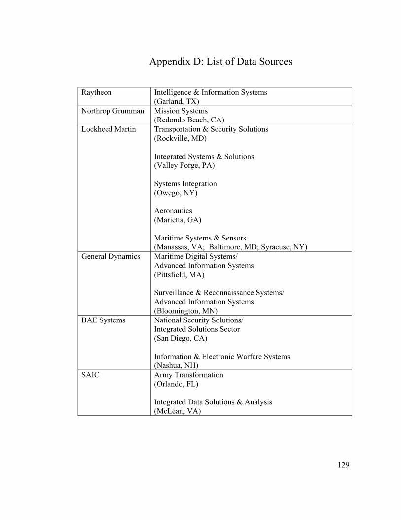
129
Appendix D: List of Data Sources Raytheon Intelligence & Information Systems
(Garland, TX) Northrop Grumman Mission Systems
(Redondo Beach, CA) Lockheed Martin Transportation & Security Solutions
(Rockville, MD) Integrated Systems & Solutions (Valley Forge, PA) Systems Integration (Owego, NY) Aeronautics (Marietta, GA) Maritime Systems & Sensors (Manassas, VA; Baltimore, MD; Syracuse, NY)
General Dynamics Maritime Digital Systems/ Advanced Information Systems (Pittsfield, MA) Surveillance & Reconnaissance Systems/ Advanced Information Systems (Bloomington, MN)
BAE Systems National Security Solutions/ Integrated Solutions Sector (San Diego, CA) Information & Electronic Warfare Systems (Nashua, NH)
SAIC Army Transformation (Orlando, FL) Integrated Data Solutions & Analysis (McLean, VA)
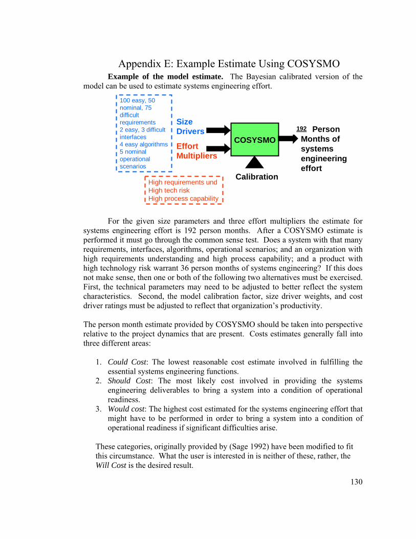
130
Appendix E: Example Estimate Using COSYSMO Example of the model estimate. The Bayesian calibrated version of the model can be used to estimate systems engineering effort.
COSYSMO
SizeDrivers
EffortMultipliers
36 Person Months of systemsengineeringeffort
Calibration
100 easy, 50 nominal, 75 difficult requirements2 easy, 3 difficult interfaces4 easy algorithms5 nominal operational scenarios
High requirements undHigh tech riskHigh process capability
For the given size parameters and three effort multipliers the estimate for systems engineering effort is 192 person months. After a COSYSMO estimate is performed it must go through the common sense test. Does a system with that many requirements, interfaces, algorithms, operational scenarios; and an organization with high requirements understanding and high process capability; and a product with high technology risk warrant 36 person months of systems engineering? If this does not make sense, then one or both of the following two alternatives must be exercised. First, the technical parameters may need to be adjusted to better reflect the system characteristics. Second, the model calibration factor, size driver weights, and cost driver ratings must be adjusted to reflect that organization’s productivity. The person month estimate provided by COSYSMO should be taken into perspective relative to the project dynamics that are present. Costs estimates generally fall into three different areas:
1. Could Cost: The lowest reasonable cost estimate involved in fulfilling the essential systems engineering functions.
2. Should Cost: The most likely cost involved in providing the systems engineering deliverables to bring a system into a condition of operational readiness.
3. Would cost: The highest cost estimated for the systems engineering effort that might have to be performed in order to bring a system into a condition of operational readiness if significant difficulties arise.
These categories, originally provided by (Sage 1992) have been modified to fit this circumstance. What the user is interested in is neither of these, rather, the Will Cost is the desired result.
192
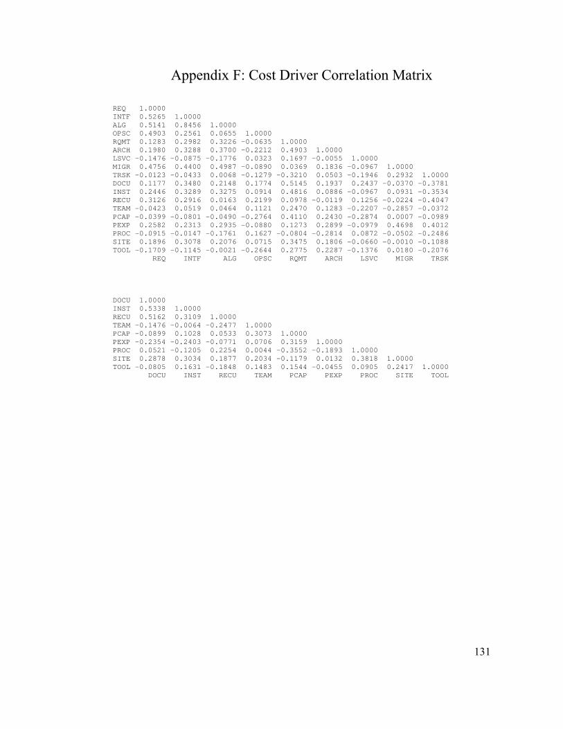
131
Appendix F: Cost Driver Correlation Matrix REQ 1.0000 INTF 0.5265 1.0000 ALG 0.5141 0.8456 1.0000 OPSC 0.4903 0.2561 0.0655 1.0000 RQMT 0.1283 0.2982 0.3226 -0.0635 1.0000 ARCH 0.1980 0.3288 0.3700 -0.2212 0.4903 1.0000 LSVC -0.1476 -0.0875 -0.1776 0.0323 0.1697 -0.0055 1.0000 MIGR 0.4756 0.4400 0.4987 -0.0890 0.0369 0.1836 -0.0967 1.0000 TRSK -0.0123 -0.0433 0.0068 -0.1279 -0.3210 0.0503 -0.1946 0.2932 1.0000 DOCU 0.1177 0.3480 0.2148 0.1774 0.5145 0.1937 0.2437 -0.0370 -0.3781 INST 0.2446 0.3289 0.3275 0.0914 0.4816 0.0886 -0.0967 0.0931 -0.3534 RECU 0.3126 0.2916 0.0163 0.2199 0.0978 -0.0119 0.1256 -0.0224 -0.4047 TEAM -0.0423 0.0519 0.0464 0.1121 0.2470 0.1283 -0.2207 -0.2857 -0.0372 PCAP -0.0399 -0.0801 -0.0490 -0.2764 0.4110 0.2430 -0.2874 0.0007 -0.0989 PEXP 0.2582 0.2313 0.2935 -0.0880 0.1273 0.2899 -0.0979 0.4698 0.4012 PROC -0.0915 -0.0147 -0.1761 0.1627 -0.0804 -0.2814 0.0872 -0.0502 -0.2486 SITE 0.1896 0.3078 0.2076 0.0715 0.3475 0.1806 -0.0660 -0.0010 -0.1088 TOOL -0.1709 -0.1145 -0.0021 -0.2644 0.2775 0.2287 -0.1376 0.0180 -0.2076 REQ INTF ALG OPSC RQMT ARCH LSVC MIGR TRSK DOCU 1.0000 INST 0.5338 1.0000 RECU 0.5162 0.3109 1.0000 TEAM -0.1476 -0.0064 -0.2477 1.0000 PCAP -0.0899 0.1028 0.0533 0.3073 1.0000 PEXP -0.2354 -0.2403 -0.0771 0.0706 0.3159 1.0000 PROC 0.0521 -0.1205 0.2254 0.0044 -0.3552 -0.1893 1.0000 SITE 0.2878 0.3034 0.1877 0.2034 -0.1179 0.0132 0.3818 1.0000 TOOL -0.0805 0.1631 -0.1848 0.1483 0.1544 -0.0455 0.0905 0.2417 1.0000 DOCU INST RECU TEAM PCAP PEXP PROC SITE TOOL
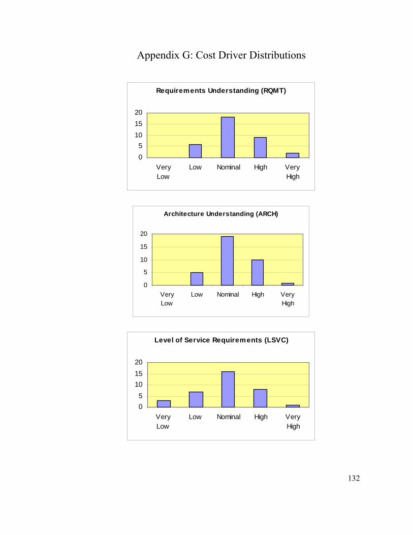
132
Appendix G: Cost Driver Distributions
Requirements Understanding (RQMT)
05
101520
VeryLow
Low Nominal High VeryHigh
Level of Service Requirements (LSVC)
05
101520
VeryLow
Low Nominal High VeryHigh
Architecture Understanding (ARCH)
0
5
10
15
20
VeryLow
Low Nominal High VeryHigh
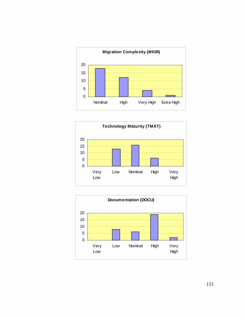
133
Migration Complexity (MIGR)
0
5
10
15
20
Nominal High Very High Extra High
Technology Maturity (TMAT)
05
101520
VeryLow
Low Nominal High VeryHigh
Documentation (DOCU)
05
101520
VeryLow
Low Nominal High VeryHigh
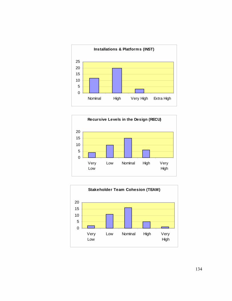
134
Installations & Platforms (INST)
05
10152025
Nominal High Very High Extra High
Recursive Levels in the Design (RECU)
05
10
1520
VeryLow
Low Nominal High VeryHigh
Stakeholder Team Cohesion (TEAM)
05
101520
VeryLow
Low Nominal High VeryHigh
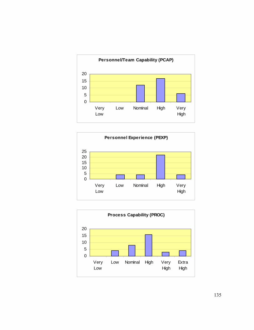
135
Personnel/Team Capability (PCAP)
05
101520
VeryLow
Low Nominal High VeryHigh
Personnel Experience (PEXP)
05
10152025
VeryLow
Low Nominal High VeryHigh
Process Capability (PROC)
05
101520
VeryLow
Low Nominal High VeryHigh
ExtraHigh
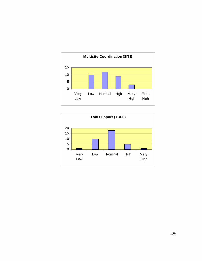
136
Multisite Coordination (SITE)
0
5
10
15
VeryLow
Low Nominal High VeryHigh
ExtraHigh
Tool Support (TOOL)
05
101520
VeryLow
Low Nominal High VeryHigh
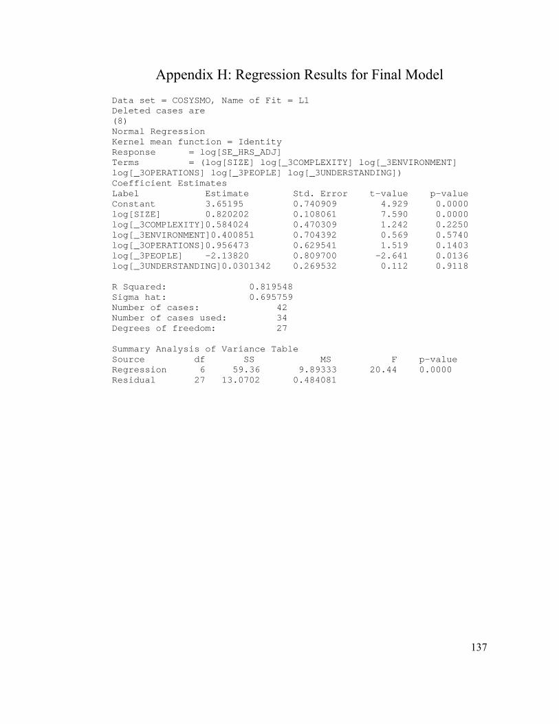
137
Appendix H: Regression Results for Final Model Data set = COSYSMO, Name of Fit = L1 Deleted cases are (8) Normal Regression Kernel mean function = Identity Response = log[SE_HRS_ADJ] Terms = (log[SIZE] log[_3COMPLEXITY] log[_3ENVIRONMENT] log[_3OPERATIONS] log[_3PEOPLE] log[_3UNDERSTANDING]) Coefficient Estimates Label Estimate Std. Error t-value p-value Constant 3.65195 0.740909 4.929 0.0000 log[SIZE] 0.820202 0.108061 7.590 0.0000 log[_3COMPLEXITY]0.584024 0.470309 1.242 0.2250 log[_3ENVIRONMENT]0.400851 0.704392 0.569 0.5740 log[_3OPERATIONS]0.956473 0.629541 1.519 0.1403 log[_3PEOPLE] -2.13820 0.809700 -2.641 0.0136 log[_3UNDERSTANDING]0.0301342 0.269532 0.112 0.9118 R Squared: 0.819548 Sigma hat: 0.695759 Number of cases: 42 Number of cases used: 34 Degrees of freedom: 27 Summary Analysis of Variance Table Source df SS MS F p-value Regression 6 59.36 9.89333 20.44 0.0000 Residual 27 13.0702 0.484081