Chapter 2

The continuous latent variablemodelling formalism

This chapter gives the theoretical basis for continuous latent variable models. Section 2.1 defines intuitivelythe concept of latent variable models and gives a brief historical introduction to them. Section 2.2 uses a simpleexample, inspired by the mechanics of a mobile point, to justify and explain latent variables. Section 2.3 givesa more rigorous definition, which we will use throughout this thesis. Section 2.6 describes the most importantspecific continuous latent variable models and section 2.7 defines mixtures of continuous latent variable models.The chapter discusses other important topics, including parameter estimation, identifiability, interpretabilityand marginalisation in high dimensions. Section 2.9 on dimensionality reduction will be the basis for part IIof the thesis. Section 2.10 very briefly mentions some applications of continuous latent variable models fordimensionality reduction. Section 2.11 shows a worked example of a simple continuous latent variable model.Section 2.12 give some complementary mathematical results, in particular the derivation of a diagonal noiseGTM model and of its EM algorithm.

2.1 Introduction and historical overview of latent variable models

Latent variable models are probabilistic models that try to explain a (relatively) high-dimensional process interms of a few degrees of freedom. Historically, the idea of latent variables arose primarily from psychometrics,beginning with the g factor of Spearman (1904) and continuing with other psychologists such as Thomson,Thurstone and Burt, who were investigating the mental ability of children as suggested by the correlation andcovariance matrices from cognitive tests variables. This eventually led to the development of factor analysis.Principal component analysis, traditionally not considered a latent variable model, was first thought of byPearson (1901) and developed as a multivariate technique by Hotelling (1933). Latent structure analysis,corresponding to models where the latent variables are categorical, originated with Lazarsfeld and Henry(1968) as a tool for sociological analysis and had a separate development from factor analysis until recently.Bartholomew (1987) gives more historical details and references.

The statistics literature classifies latent variable models according to the metric (continuous) or categorical(discrete) character of the variables involved, as table 2.1 shows. Also, in a broad sense many probabilisticmodels commonly used in machine learning can be considered as latent variable models inasmuch as theyinclude probability distributions for variables which are not observed: mixture models (where the variablewhich indexes the components is a latent variable), hidden Markov models (the state sequence is unobserved),

This chapter is an extended version of references Carreira-Perpinan (1996, 1997).

Observed variablesMetrical Categorical

Metrical Factor analysis Latent trait analysisLatent

variables CategoricalLatent profile analysis Latent class analysis

Analysis of mixtures

Table 2.1: Classification of latent variable models (adapted from Bartholomew, 1987).

5

Helmholtz machines (Dayan et al., 1995) (the activations of each unit), elastic nets (Durbin et al., 1989) (thetour knots), etc. In this chapter we will concentrate exclusively on latent variable models where both thelatent and the observed variables are continuous (although much of the general treatment applies to discretevariables too), going much further than the linear-normal model of factor analysis. In some points discretevariables will appear as a result of a Monte Carlo discretisation. The latent class model where the observedvariables are binary and there is a single discrete latent variable corresponds to the mixture of multivariateBernoulli distributions, which is discussed in chapter 3 and used in chapter 5.

In this work, we follow (with minor variations) the theoretical framework currently accepted in statistics forlatent variable models, for which two good references are Everitt (1984) and Bartholomew (1987). However,these works do not include any of the more recent latent variable models such as GTM, ICA or IFA, and theydo not discuss issues of importance in machine learning, such as the continuity of the dimensionality reductionmapping or the mixtures of continuous latent variable models. The work of MacKay (1995a) on densitynetworks, which is the name he uses for nonlinear latent variable models, was pioneering in the introduction ofthe latent variable model framework to the machine learning community (in spite of an odd choice of journal).

The traditional treatment of latent variable models in the statistics literature is (Krzanowski, 1988):

1. formulate model (independence and distributional assumptions)

2. estimate parameters (by maximum likelihood)

3. test hypotheses about the parameters

which perhaps explains why most of the statistical research on latent variables has remained in the linear-normal model of factor analysis (with a few exceptions, e.g. the use of polynomial rather than linear functions;Etezadi-Amoli and McDonald, 1983; McDonald, 1985): rigorous analysis of nonlinear models is very difficult.Interesting developments concerning new models and learning algorithms have appeared in the literature ofstatistical pattern recognition in the 1990s, as the rest of this chapter will show.

Traditionally, most applications of latent variables have been in psychology and the social sciences, wherehypothesised latent variables such as intelligence, verbal ability or social class are believed to exist; they havebeen less used in the natural sciences, where often most variables are measurable (Krzanowski, 1988, p. 502).This latter statement is not admissible under the generative point of view exposed in sections 2.2 and 2.3,whereby the processes of measurement and stochastic variation (noise) can make a physical system appearmore high-dimensional than it really is. In fact, factor analysis has been applied to a number of “naturalscience” problems (e.g. in botany, biology, geology or engineering) as well as other kinds of latent variablemodels recently developed, such as the application of GTM to dimensionality reduction of electropalatographicdata (Carreira-Perpinan and Renals, 1998a) or of ICA to the removal of artifacts in electroencephalographicrecordings (Makeig et al., 1997). Besides that, the most popular technique for dimensionality reduction,principal component analysis, has recently been recast in the form of a particular kind of factor analysis—thusas a latent variable model.

Whether the latent variables revealed can or cannot be interpreted (a delicate issue discussed in sec-tion 2.8.1), latent variable models are a powerful tool for data analysis when the intrinsic dimensionality ofthe problem is smaller than the apparent one and they are specially suited for dimensionality reduction andmissing data reconstruction—as this thesis will try to demonstrate.

2.2 Physical interpretation of the latent variable model formalism

In this section we give a physical flavour to the generative view of latent variables. This generative view willbe properly defined in section 2.3 and should be compared to the physical interpretation given below.

2.2.1 An example: eclipsing spectroscopic binary star

We will introduce the idea of latent variables through an example from astronomy, that of eclipsing spectroscopicbinary stars (Roy, 1978). A binary system is a pair of stars that describe orbits about their common centre ofmass, the two components being gravitationally bound together. An eclipsing spectroscopic binary is viewedas a single star because the components are so close that they cannot be resolved in a telescope, but its doublenature can be revealed in several ways:

• If the orbit plane contains or is close to the line of sight, the components will totally or partially eclipseeach other, which results in regular diminutions in the binary star’s brightness.

6

• The Doppler effect1 of the orbital velocities of the components produces shifts to red and blue on thespectral lines of the binary star.

A well-known example of this kind of star system is Algol (β Per), which is actually a ternary system.We will consider a simplified model of eclipsing spectroscopic binary star, in which one star (the primary

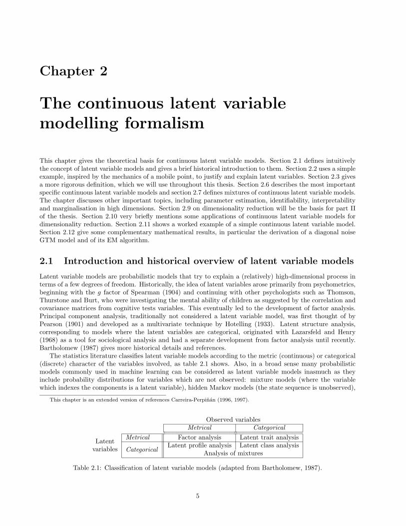
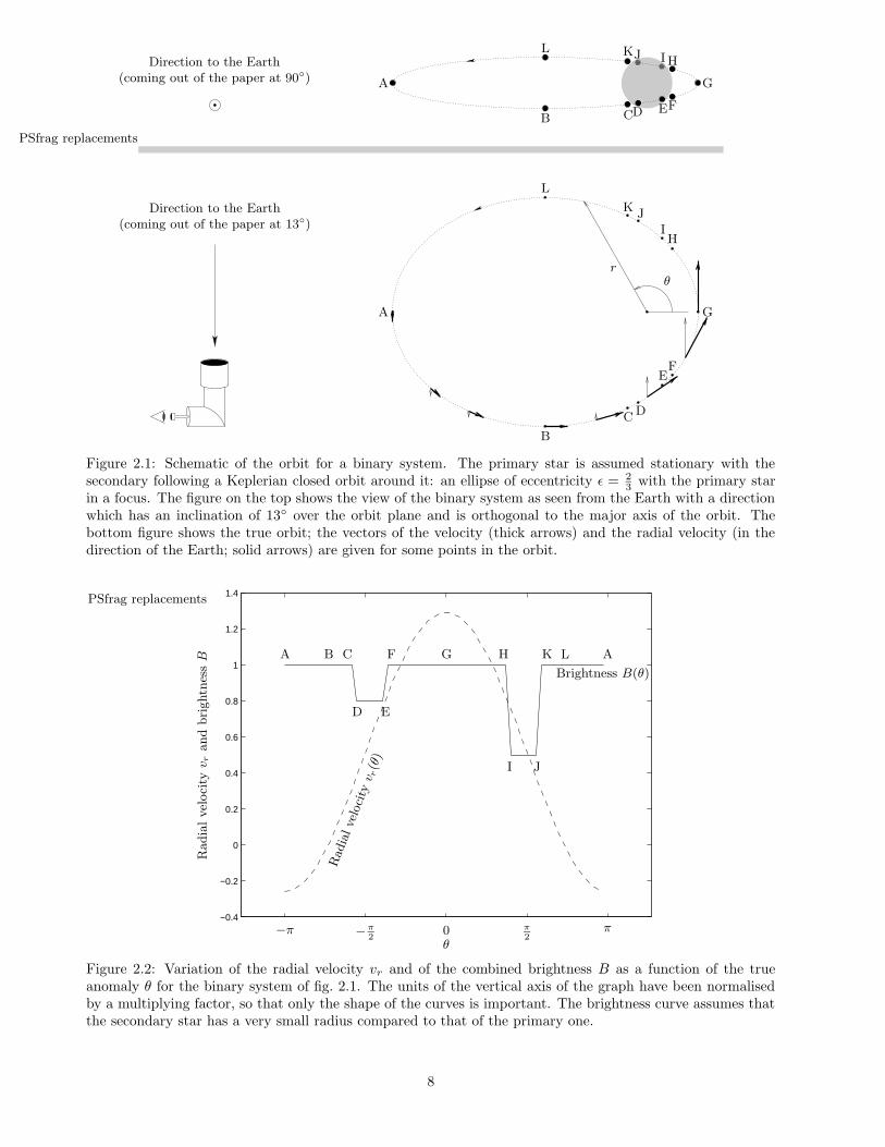
star) is much more massive than the other, thus remaining practically stationary in the centre-of-mass system.The secondary star follows an elliptical orbit around the primary one, which is located at one of the foci.Figures 2.1 and 2.2 show the trajectory of the secondary star and the basic form of the variation with thepolar angle θ (true anomaly) of:

• The radial velocity vr of the secondary star (i.e., the projection of the velocity vector along the lineof sight from the Earth), to which the spectrum shift is proportional. We are assuming a stationaryobserver in Earth, so that the measured radial velocity must be corrected for the Earth’s orbital motionabout the Sun.

• The combined brightness B.

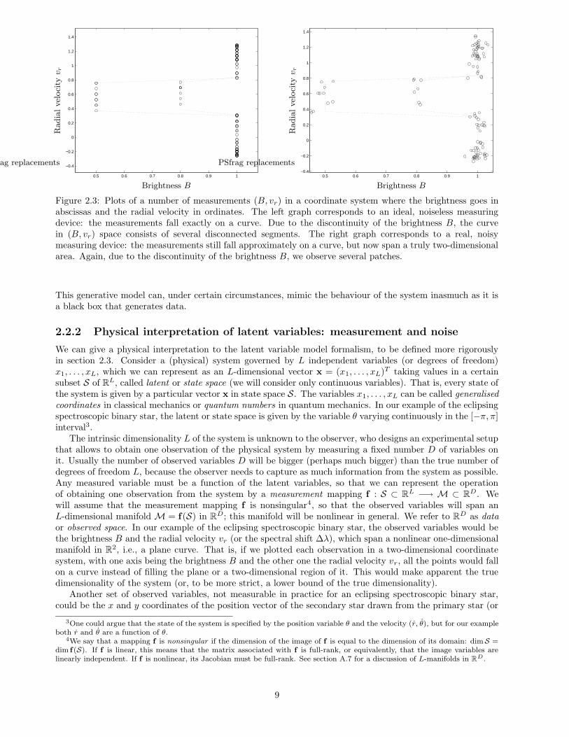
We would like to provide a scenario which, though idealised, is very close to an experimental situation thatan astronomer could find. Thus, we are ignoring complicated effects, such as the facts that: the shape of bothstars can be far from spherical, as they can fill their lobes (bounded by the Roche limit); the stars do nothave uniform brightness across their discs, but decreasing towards the limb (limb darkening); the relativisticadvance of the periastron with time; the perturbation due to third bodies; etc. Thus, the true theoreticalcurve for the brightness will not be piecewise linear and the actual curve will vary from one binary system toanother, but it will always conserve the form indicated in fig. 2.2: a periodic curve with two falls correspondingto the eclipses. Similarly, the spectral shift will be a periodic oscillating function.

Now, an astronomer could collect a number of paired measurements (B, vr) and construct with thembrightness and radial velocity (or spectrum) curves such as those of fig. 2.2 (although perhaps replacingthe true anomaly θ by a more natural variable in this case, such as the time t at which the measurementwas collected). Detailed analysis of the brightness and spectrum curves under the laws of Kepler can provideknowledge of the eccentricity and inclination of the orbit, the major semiaxis, the radii, masses and luminositiesof the stars, etc.

The knowledge of the astronomer that all measured variables (B and vr) depend on a single variable, thetrue anomaly θ, is implicit. That is, given θ, the configuration of the binary system is completely defined andso are the values of all the variables we could measure: B, vr, even r, etc.

Now let us suppose that we have such a collection of measurements but that we do not know anything aboutthe underlying model that generated them, i.e., we do not know that the observed brightness and spectral shiftsare (indirectly) governed by Kepler’s law. Let us consider the following question: could it be possible that,although we are measuring two variables each time we observe the system, just one variable (not necessarily Bor vr) would be enough to determine the configuration of the system completely?2 More concisely: could thenumber of degrees of freedom of the binary system be smaller than the number of variables that we measurefrom it?

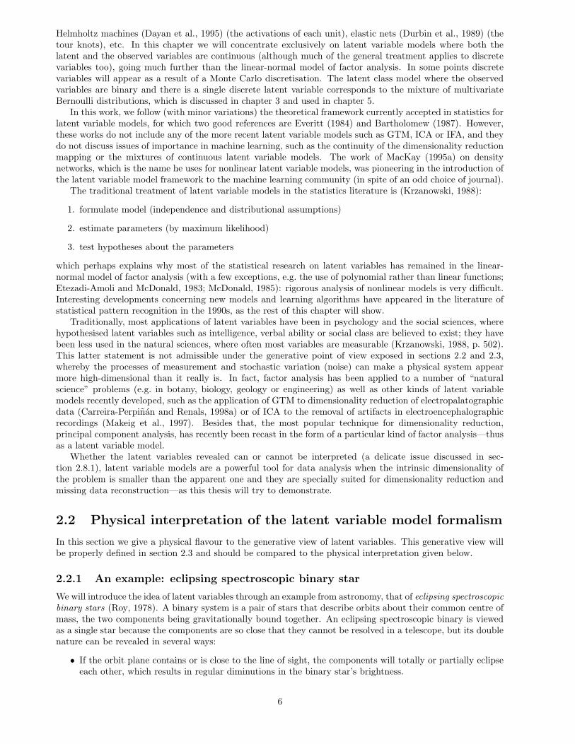
As we discuss in section 4.4, this is a very difficult question to answer if the measurements are corrupted bynoise or if each measurement consists of more than about 3 variables. But if we plotted the collection of pairs(B, vr) in a plane coordinate system, with each variable being associated with one axis, we would observe thefollowing fact (fig. 2.3 left): the points do not fall all over the plane, spanning an extensional (two-dimensional)area, but fall on a curve (dotted in the figure). If we accept that our instruments are imperfect, so that eachpoint is slightly off the position where it should be, we would observe a situation like that of fig. 2.3 right: thepoints now occupy an extensional area (several oval patches), but it is apparent that the region over which themeasurements fall is still a curve. This gives away the fact that the system has only one degree of freedom,however many different, apparently unrelated variables we want to measure from it. In this example, theintrinsic dimensionality of the binary system is one but we measure two variables.

Accepting that the intrinsic dimensionality of a system is smaller than the number of variables that wemeasure from it, the latent variable framework allows the construction of a generative model for the system.

1If a source emitting radiation has a velocity v relative to the observer, the received radiation that normally has a wavelength

λ when the velocity relative to the observer is 0 will have a measured wavelength λ′ with λ′−λλ

= vc, where c is the speed of light

and the source is approaching for v < 0 and receding for v > 0. Thus, the Doppler shift is defined as ∆λλ

= vc, being positive for

red shift and negative for blue shift.2Of course we could argue that two variables could not be enough to determine the system configuration completely, but we

will suppose that this is not the case.

7

PSfrag replacements

A

A

B

B

C

C

D

D

E

E

F

F

G

G

H

H

I

I

J

J

K

K

L

LDirection to the Earth

(coming out of the paper at 90◦)

Direction to the Earth(coming out of the paper at 13◦)

rθ

Figure 2.1: Schematic of the orbit for a binary system. The primary star is assumed stationary with thesecondary following a Keplerian closed orbit around it: an ellipse of eccentricity ε = 2

3 with the primary starin a focus. The figure on the top shows the view of the binary system as seen from the Earth with a directionwhich has an inclination of 13◦ over the orbit plane and is orthogonal to the major axis of the orbit. Thebottom figure shows the true orbit; the vectors of the velocity (thick arrows) and the radial velocity (in thedirection of the Earth; solid arrows) are given for some points in the orbit.

−0.4

−0.2

0

0.2

0.4

0.6

0.8

1

1.2

1.4PSfrag replacements

AA B C

D E

F G H

I J

K L

−π −π2

0 π2

π

θ

Radia

lvel

oci

tyv

rand

bri

ghtn

ess

B

Rad

ialve

loci

tyv r

(θ)

Brightness B(θ)

Figure 2.2: Variation of the radial velocity vr and of the combined brightness B as a function of the trueanomaly θ for the binary system of fig. 2.1. The units of the vertical axis of the graph have been normalisedby a multiplying factor, so that only the shape of the curves is important. The brightness curve assumes thatthe secondary star has a very small radius compared to that of the primary one.

8

0.5 0.6 0.7 0.8 0.9 1

−0.4

−0.2

0

0.2

0.4

0.6

0.8

1

1.2

1.4

PSfrag replacements

Brightness B

Radia

lvel

oci

tyv

r

0.5 0.6 0.7 0.8 0.9 1−0.4

−0.2

0

0.2

0.4

0.6

0.8

1

1.2

1.4

PSfrag replacements

Brightness B

Radia

lvel

oci

tyv

r

Figure 2.3: Plots of a number of measurements (B, vr) in a coordinate system where the brightness goes inabscissas and the radial velocity in ordinates. The left graph corresponds to an ideal, noiseless measuringdevice: the measurements fall exactly on a curve. Due to the discontinuity of the brightness B, the curvein (B, vr) space consists of several disconnected segments. The right graph corresponds to a real, noisymeasuring device: the measurements still fall approximately on a curve, but now span a truly two-dimensionalarea. Again, due to the discontinuity of the brightness B, we observe several patches.

This generative model can, under certain circumstances, mimic the behaviour of the system inasmuch as it isa black box that generates data.

2.2.2 Physical interpretation of latent variables: measurement and noise

We can give a physical interpretation to the latent variable model formalism, to be defined more rigorouslyin section 2.3. Consider a (physical) system governed by L independent variables (or degrees of freedom)x1, . . . , xL, which we can represent as an L-dimensional vector x = (x1, . . . , xL)T taking values in a certainsubset S of RL, called latent or state space (we will consider only continuous variables). That is, every state ofthe system is given by a particular vector x in state space S. The variables x1, . . . , xL can be called generalisedcoordinates in classical mechanics or quantum numbers in quantum mechanics. In our example of the eclipsingspectroscopic binary star, the latent or state space is given by the variable θ varying continuously in the [−π, π]interval3.

The intrinsic dimensionality L of the system is unknown to the observer, who designs an experimental setupthat allows to obtain one observation of the physical system by measuring a fixed number D of variables onit. Usually the number of observed variables D will be bigger (perhaps much bigger) than the true number ofdegrees of freedom L, because the observer needs to capture as much information from the system as possible.Any measured variable must be a function of the latent variables, so that we can represent the operationof obtaining one observation from the system by a measurement mapping f : S ⊂ RL −→ M ⊂ RD. Wewill assume that the measurement mapping f is nonsingular4, so that the observed variables will span anL-dimensional manifold M = f(S) in RD; this manifold will be nonlinear in general. We refer to RD as dataor observed space. In our example of the eclipsing spectroscopic binary star, the observed variables would bethe brightness B and the radial velocity vr (or the spectral shift ∆λ), which span a nonlinear one-dimensionalmanifold in R2, i.e., a plane curve. That is, if we plotted each observation in a two-dimensional coordinatesystem, with one axis being the brightness B and the other one the radial velocity vr, all the points would fallon a curve instead of filling the plane or a two-dimensional region of it. This would make apparent the truedimensionality of the system (or, to be more strict, a lower bound of the true dimensionality).

Another set of observed variables, not measurable in practice for an eclipsing spectroscopic binary star,could be the x and y coordinates of the position vector of the secondary star drawn from the primary star (or

3One could argue that the state of the system is specified by the position variable θ and the velocity (r, θ), but for our exampleboth r and θ are a function of θ.

4We say that a mapping f is nonsingular if the dimension of the image of f is equal to the dimension of its domain: dimS =dim f(S). If f is linear, this means that the matrix associated with f is full-rank, or equivalently, that the image variables arelinearly independent. If f is nonlinear, its Jacobian must be full-rank. See section A.7 for a discussion of L-manifolds in RD.

9

PSfrag replacements

O

PQ

r

r + dr

dθ

r dθ uθ

dr urdr

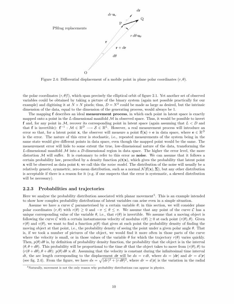
Figure 2.4: Differential displacement of a mobile point in plane polar coordinates (r, θ).

the polar coordinates (r, θ)!), which span precisely the elliptical orbit of figure 2.1. Yet another set of observedvariables could be obtained by taking a picture of the binary system (again not possible practically for ourexample) and digitising it at N ×N pixels; thus, D = N 2 could be made as large as desired, but the intrinsicdimension of the data, equal to the dimension of the generating process, would always be 1.

The mapping f describes an ideal measurement process, in which each point in latent space is exactlymapped onto a point in the L-dimensional manifoldM in observed space. Thus, it would be possible to invertf and, for any point in M, recover its corresponding point in latent space (again assuming that L < D andthat f is invertible): f−1 : M ∈ RD −→ S ∈ RL. However, a real measurement process will introduce anerror so that, for a latent point x, the observer will measure a point f(x) + e in data space, where e ∈ RD

is the error. The nature of this error is stochastic, i.e., repeated measurements of the system being in thesame state would give different points in data space, even though the mapped point would be the same. Themeasurement error will hide to some extent the true, low-dimensional nature of the data, transforming theL-dimensional manifold M into a D-dimensional region in data space. The higher the error level, the moredistortion M will suffer. It is customary to refer to this error as noise. We can assume that it follows acertain probability law, prescribed by a density function p(t|x), which gives the probability that latent pointx will be observed as data point t; we call this the noise model. The distribution of the noise will usually be arelatively generic, symmetric, zero-mean distribution, such as a normal N (f(x),Σ), but any other distributionis acceptable if there is a reason for it (e.g. if one suspects that the error is systematic, a skewed distributionwill be necessary).

2.2.3 Probabilities and trajectories

Here we analyse the probability distribution associated with planar movement5. This is an example intendedto show how complex probability distributions of latent variables can arise even in a simple situation.

Assume we have a curve C parameterised by a certain variable θ; in this section, we will consider planepolar coordinates (r, θ) with r(θ) ≥ 0 and −π ≤ θ ≤ π. We assume that any point of the curve C has aunique corresponding value of the variable θ, i.e., that r(θ) is invertible. We assume that a moving object isfollowing the curve C with a certain instantaneous velocity of modulus v(θ) ≥ 0 at each point (r(θ), θ). Givenr(θ) and v(θ), we want to find a function p(θ) that gives at each point the probability density of finding themoving object at that point, i.e., the probability density of seeing the point under a given polar angle θ. Thatis, if we took a number of pictures of the object, we would find it more often in those parts of the curvewhere the velocity is small, or in those values of the variable θ for which the trajectory r(θ) varies quickly.Then, p(θ) dθ is, by definition of probability density function, the probability that the object is in the interval(θ, θ+ dθ). This probability will be proportional to the time dt that the object takes to move from (r(θ), θ) to(r(θ + dθ), θ + dθ): p(θ) dθ ∝ dt. Assuming that the velocity is constant during the infinitesimal time intervaldt, the arc length corresponding to the displacement dr will be ds = v dt, where ds = |dr| and dr = d |r|(see fig. 2.4). From the figure, we have ds =

√

(dr)2 + (r dθ)2, where dr = d |r| is the variation in the radial

5Naturally, movement is not the only reason why probability distributions can appear in physics.

10

0.53333

1.0667

1.6

30

210

60

240

90

270

120

300

150

330

180 0

PSfrag replacements−π−π

20π2πθ

r(θ), v(θ), p(θ)

PSfrag replacements

−π −π2

0 π2

π

θ

r(θ

),v(θ

),p(θ

)

0.53333

1.0667

1.6

30

210

60

240

90

270

120

300

150

330

180 0

PSfrag replacements−π−π

20π2πθ

r(θ), v(θ), p(θ)

PSfrag replacements

−π −π2

0 π2

π

θ

r(θ

),v(θ

),p(θ

)

0.53333

1.0667

1.6

30

210

60

240

90

270

120

300

150

330

180 0

PSfrag replacements−π−π

20π2πθ

r(θ), v(θ), p(θ)

PSfrag replacements

−π −π2

0 π2

π

θ

r(θ

),v(θ

),p(θ

)

0.53333

1.0667

1.6

30

210

60

240

90

270

120

300

150

330

180 0

PSfrag replacements−π−π

20π2πθ

r(θ), v(θ), p(θ)

PSfrag replacements

−π −π2

0 π2

π

θ

r(θ

),v(θ

),p(θ

)

0.53333

1.0667

1.6

30

210

60

240

90

270

120

300

150

330

180 0

PSfrag replacements−π−π

20π2πθ

r(θ), v(θ), p(θ)

PSfrag replacements

−π −π2

0 π2

π

θ

r(θ

),v(θ

),p(θ

)

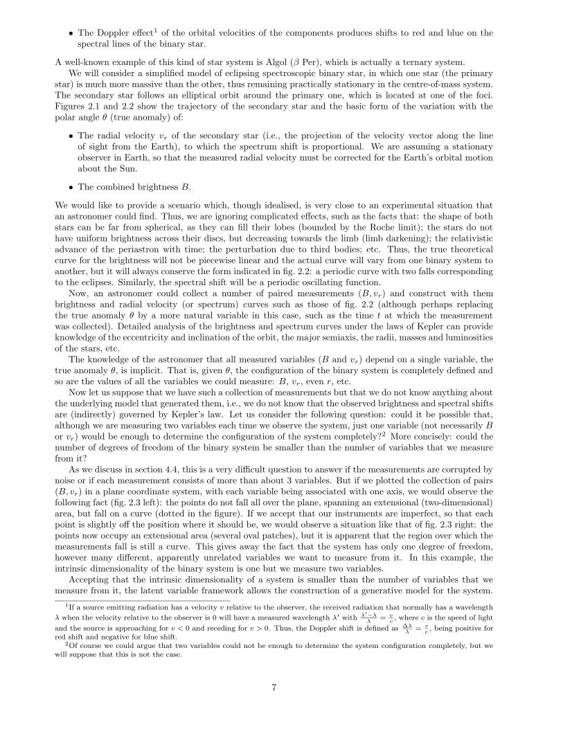
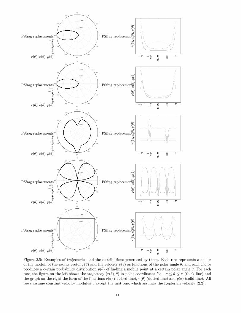
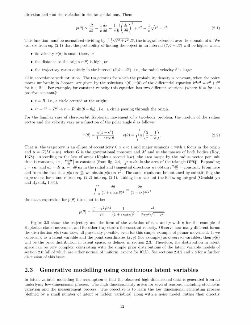
Figure 2.5: Examples of trajectories and the distributions generated by them. Each row represents a choiceof the moduli of the radius vector r(θ) and the velocity v(θ) as functions of the polar angle θ, and each choiceproduces a certain probability distribution p(θ) of finding a mobile point at a certain polar angle θ. For eachrow, the figure on the left shows the trajectory (r(θ), θ) in polar coordinates for −π ≤ θ ≤ π (thick line) andthe graph on the right the form of the functions r(θ) (dashed line), v(θ) (dotted line) and p(θ) (solid line). Allrows assume constant velocity modulus v except the first one, which assumes the Keplerian velocity (2.2).

11

direction and r dθ the variation in the tangential one. Then:

p(θ) ∝ dt

dθ=

1

v

ds

dθ=

1

v

√(dr

dθ

)2

+ r2 =1

v

√

r2 + r2. (2.1)

This function must be normalised dividing by∫

1v

√r2 + r2 dθ, the integral extended over the domain of θ. We

can see from eq. (2.1) that the probability of finding the object in an interval (θ, θ + dθ) will be higher when:

• its velocity v(θ) is small there, or

• the distance to the origin r(θ) is high, or

• the trajectory varies quickly in the interval (θ, θ + dθ), i.e., the radial velocity r is large;

all in accordance with intuition. The trajectories for which the probability density is constant, when the pointmoves uniformly in θ-space, are given by the solutions r(θ), v(θ) of the differential equation k2v2 = r2 + r2

for k ∈ R+. For example, for constant velocity this equation has two different solutions (where R = kv is apositive constant):

• r = R, i.e., a circle centred at the origin;

• r2 + r2 = R2 ⇒ r = R |sin(θ − θ0)|, i.e., a circle passing through the origin.

For the familiar case of closed-orbit Keplerian movement of a two-body problem, the moduli of the radiusvector and the velocity vary as a function of the polar angle θ as follows:

r(θ) =a(1− ε2)1 + ε cos θ

v(θ) =

√

µ

(2

r− 1

a

)

. (2.2)

That is, the trajectory is an ellipse of eccentricity 0 ≤ ε < 1 and major semiaxis a with a focus in the originand µ = G(M + m), where G is the gravitational constant and M and m the masses of both bodies (Roy,1978). According to the law of areas (Kepler’s second law), the area swept by the radius vector per unittime is constant, i.e.,

∣∣ r×drdt

∣∣ = constant (from fig. 2.4,

∣∣ 12r× dr

∣∣ is the area of the triangle OPQ). Expanding

r = rur and dr = dr ur + r dθ uθ in the radial and tangential directions we obtain r2 dθdt = constant. From here

and from the fact that p(θ) ∝ dtdθ we obtain p(θ) ∝ r2. The same result can be obtained by substituting the

expressions for v and r from eq. (2.2) into eq. (2.1). Taking into account the following integral (Gradshteynand Ryzhik, 1994):

∫ π

−π

dθ

(1 + ε cos θ)2=

2π

(1− ε2)3/2 ,

the exact expression for p(θ) turns out to be:

p(θ) =(1− ε2)3/2

2π

1

(1 + ε cos θ)2=

r2

2πa2√

1− ε2.

Figure 2.5 shows the trajectory and the form of the variation of r, v and p with θ for the example ofKeplerian closed movement and for other trajectories for constant velocity. Observe how many different formsthe distribution p(θ) can take, all physically possible, even for this simple example of planar movement. If weconsider θ as a latent variable and the point coordinates (x, y) (for example) as observed variables, then p(θ)will be the prior distribution in latent space, as defined in section 2.3. Therefore, the distribution in latentspace can be very complex, contrasting with the simple prior distributions of the latent variable models ofsection 2.6 (all of which are either normal of uniform, except for ICA). See sections 2.3.2 and 2.8 for a furtherdiscussion of this issue.

2.3 Generative modelling using continuous latent variables

In latent variable modelling the assumption is that the observed high-dimensional data is generated from anunderlying low-dimensional process. The high dimensionality arises for several reasons, including stochasticvariation and the measurement process. The objective is to learn the low dimensional generating process(defined by a small number of latent or hidden variables) along with a noise model, rather than directly

12

PSfrag replacements

x1

x2 x

Latent space X of dimension L = 2

Prior p(x)

f

Induced p(t)

t1

t2

t3

t

f(x)

Data space T of dimension D = 3

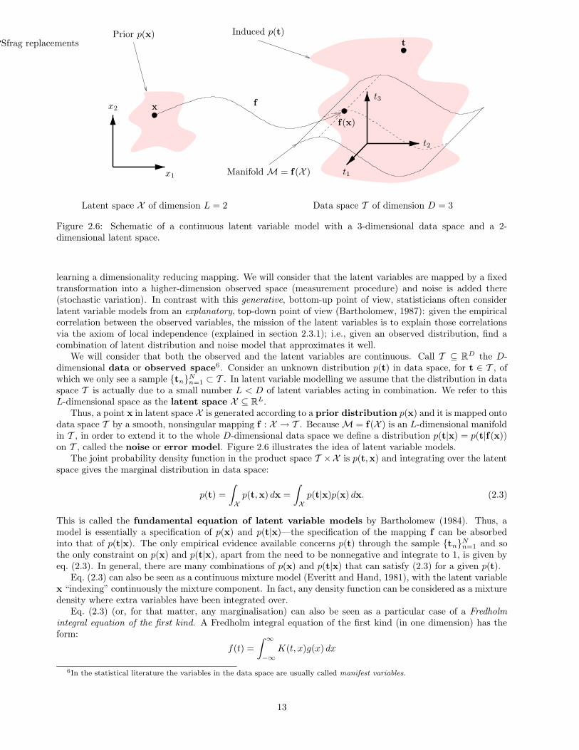
Manifold M = f(X )

Figure 2.6: Schematic of a continuous latent variable model with a 3-dimensional data space and a 2-dimensional latent space.

learning a dimensionality reducing mapping. We will consider that the latent variables are mapped by a fixedtransformation into a higher-dimension observed space (measurement procedure) and noise is added there(stochastic variation). In contrast with this generative, bottom-up point of view, statisticians often considerlatent variable models from an explanatory, top-down point of view (Bartholomew, 1987): given the empiricalcorrelation between the observed variables, the mission of the latent variables is to explain those correlationsvia the axiom of local independence (explained in section 2.3.1); i.e., given an observed distribution, find acombination of latent distribution and noise model that approximates it well.

We will consider that both the observed and the latent variables are continuous. Call T ⊆ RD the D-dimensional data or observed space6. Consider an unknown distribution p(t) in data space, for t ∈ T , ofwhich we only see a sample {tn}Nn=1 ⊂ T . In latent variable modelling we assume that the distribution in dataspace T is actually due to a small number L < D of latent variables acting in combination. We refer to thisL-dimensional space as the latent space X ⊆ RL.

Thus, a point x in latent space X is generated according to a prior distribution p(x) and it is mapped ontodata space T by a smooth, nonsingular mapping f : X → T . BecauseM = f(X ) is an L-dimensional manifoldin T , in order to extend it to the whole D-dimensional data space we define a distribution p(t|x) = p(t|f(x))on T , called the noise or error model. Figure 2.6 illustrates the idea of latent variable models.

The joint probability density function in the product space T ×X is p(t,x) and integrating over the latentspace gives the marginal distribution in data space:

p(t) =

∫

Xp(t,x) dx =

∫

Xp(t|x)p(x) dx. (2.3)

This is called the fundamental equation of latent variable models by Bartholomew (1984). Thus, amodel is essentially a specification of p(x) and p(t|x)—the specification of the mapping f can be absorbedinto that of p(t|x). The only empirical evidence available concerns p(t) through the sample {tn}Nn=1 and sothe only constraint on p(x) and p(t|x), apart from the need to be nonnegative and integrate to 1, is given byeq. (2.3). In general, there are many combinations of p(x) and p(t|x) that can satisfy (2.3) for a given p(t).

Eq. (2.3) can also be seen as a continuous mixture model (Everitt and Hand, 1981), with the latent variablex “indexing” continuously the mixture component. In fact, any density function can be considered as a mixturedensity where extra variables have been integrated over.

Eq. (2.3) (or, for that matter, any marginalisation) can also be seen as a particular case of a Fredholmintegral equation of the first kind. A Fredholm integral equation of the first kind (in one dimension) has theform:

f(t) =

∫ ∞

−∞K(t, x)g(x) dx

6In the statistical literature the variables in the data space are usually called manifest variables.

13

PSfrag replacements

x x1 x2

td te t1 t2 t3 t4 t5

latent variables

observed variables

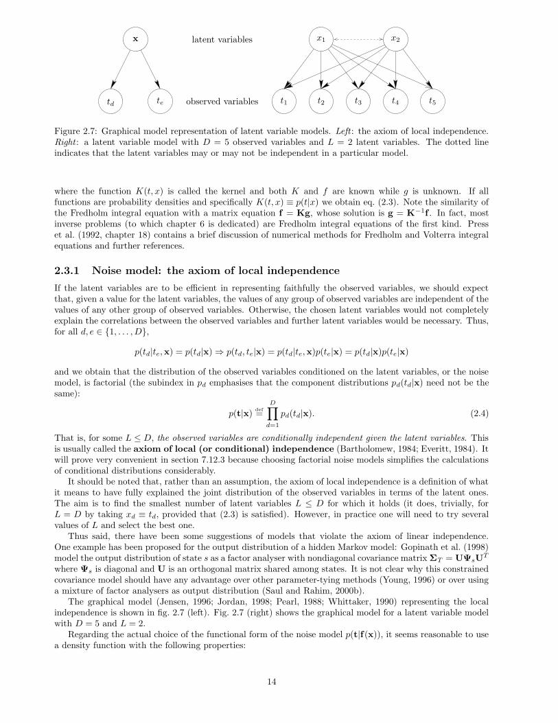
Figure 2.7: Graphical model representation of latent variable models. Left : the axiom of local independence.Right : a latent variable model with D = 5 observed variables and L = 2 latent variables. The dotted lineindicates that the latent variables may or may not be independent in a particular model.

where the function K(t, x) is called the kernel and both K and f are known while g is unknown. If allfunctions are probability densities and specifically K(t, x) ≡ p(t|x) we obtain eq. (2.3). Note the similarity ofthe Fredholm integral equation with a matrix equation f = Kg, whose solution is g = K−1f . In fact, mostinverse problems (to which chapter 6 is dedicated) are Fredholm integral equations of the first kind. Presset al. (1992, chapter 18) contains a brief discussion of numerical methods for Fredholm and Volterra integralequations and further references.

2.3.1 Noise model: the axiom of local independence

If the latent variables are to be efficient in representing faithfully the observed variables, we should expectthat, given a value for the latent variables, the values of any group of observed variables are independent of thevalues of any other group of observed variables. Otherwise, the chosen latent variables would not completelyexplain the correlations between the observed variables and further latent variables would be necessary. Thus,for all d, e ∈ {1, . . . , D},

p(td|te,x) = p(td|x)⇒ p(td, te|x) = p(td|te,x)p(te|x) = p(td|x)p(te|x)

and we obtain that the distribution of the observed variables conditioned on the latent variables, or the noisemodel, is factorial (the subindex in pd emphasises that the component distributions pd(td|x) need not be thesame):

p(t|x)def=

D∏

d=1

pd(td|x). (2.4)

That is, for some L ≤ D, the observed variables are conditionally independent given the latent variables. Thisis usually called the axiom of local (or conditional) independence (Bartholomew, 1984; Everitt, 1984). Itwill prove very convenient in section 7.12.3 because choosing factorial noise models simplifies the calculationsof conditional distributions considerably.

It should be noted that, rather than an assumption, the axiom of local independence is a definition of whatit means to have fully explained the joint distribution of the observed variables in terms of the latent ones.The aim is to find the smallest number of latent variables L ≤ D for which it holds (it does, trivially, forL = D by taking xd ≡ td, provided that (2.3) is satisfied). However, in practice one will need to try severalvalues of L and select the best one.

Thus said, there have been some suggestions of models that violate the axiom of linear independence.One example has been proposed for the output distribution of a hidden Markov model: Gopinath et al. (1998)model the output distribution of state s as a factor analyser with nondiagonal covariance matrix ΣT = UΨsU

T

where Ψs is diagonal and U is an orthogonal matrix shared among states. It is not clear why this constrainedcovariance model should have any advantage over other parameter-tying methods (Young, 1996) or over usinga mixture of factor analysers as output distribution (Saul and Rahim, 2000b).

The graphical model (Jensen, 1996; Jordan, 1998; Pearl, 1988; Whittaker, 1990) representing the localindependence is shown in fig. 2.7 (left). Fig. 2.7 (right) shows the graphical model for a latent variable modelwith D = 5 and L = 2.

Regarding the actual choice of the functional form of the noise model p(t|f(x)), it seems reasonable to usea density function with the following properties:

14

PSfrag replacements

−1

−1−1

−1−1

−1 −2−3

1

1

1

11

1

2 3t1 t′1 t′′1

t2 t′2 t′′22σ

tdef∼ 1

2N((

−10

),(

σ2 00 1

))

+ 12N

((10

),(

σ2 00 1

))

µ = 0, Σ =(

σ2+1 00 1

)

Sphering t′def= Σ−1/2(t − µ)

t′ ∼ 12N

((

−(σ2+1)−1/2

0

)

,(

σ2(σ2+1)−1 00 1

))

+ 12N

((

(σ2+1)−1/2

0

)

,(

σ2(σ2+1)−1 00 1

))

µ′ = 0, Σ′ = I

Transformation t′′def=(

σ−1 00 1

)

(t − µ)

t′′ ∼ 12N

((

−σ−1

0

)

, I)

+ 12N

((

σ−1

0

)

, I)

µ′′ = 0, Σ′′ =(

σ−2(σ2+1) 00 1

)

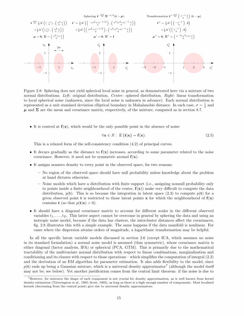
Figure 2.8: Sphering does not yield spherical local noise in general, as demonstrated here via a mixture of twonormal distributions. Left : original distribution. Centre: sphered distribution. Right : linear transformationto local spherical noise (unknown, since the local noise is unknown in advance). Each normal distribution isrepresented as a unit standard deviation elliptical boundary in Mahalanobis distance. In each case, σ = 1

2 andµ and Σ are the mean and covariance matrix, respectively, of the mixture, computed as in section 8.7.

• It is centred at f(x), which would be the only possible point in the absence of noise:

∀x ∈ X : E {t|x} = f(x). (2.5)

This is a relaxed form of the self-consistency condition (4.2) of principal curves.

• It decays gradually as the distance to f(x) increases, according to some parameter related to the noisecovariance. However, it need not be symmetric around f(x).

• It assigns nonzero density to every point in the observed space, for two reasons:

– No region of the observed space should have null probability unless knowledge about the problemat hand dictates otherwise.

– Noise models which have a distribution with finite support (i.e., assigning nonnull probability onlyto points inside a finite neighbourhood of the centre, f(x)) make very difficult to compute the datadistribution, p(t). This is so because the integration in latent space (2.3) to compute p(t) for agiven observed point t is restricted to those latent points x for which the neighbourhood of f(x)contains t (so that p(t|x) > 0).

• It should have a diagonal covariance matrix to account for different scales in the different observedvariables t1, . . . , tD. This latter aspect cannot be overcome in general by sphering the data and using anisotropic noise model, because if the data has clusters, the intercluster distances affect the covariances;fig. 2.8 illustrates this with a simple example. The same happens if the data manifold is nonlinear. Forcases where the dispersion attains orders of magnitude, a logarithmic transformation may be helpful.

In all the specific latent variable models discussed in section 2.6 (except ICA, which assumes no noisein its standard formulation) a normal noise model is assumed (thus symmetric), whose covariance matrix iseither diagonal (factor analysis, IFA) or spherical (PCA, GTM). This is primarily due to the mathematicaltractability of the multivariate normal distribution with respect to linear combinations, marginalisation andconditioning and its closure with respect to those operations—which simplifies the computation of integral (2.3)and the derivation of an EM algorithm for parameter estimation. It also adds flexibility to the model, sincep(t) ends up being a Gaussian mixture, which is a universal density approximator7 (although the model itselfmay not be; see below). Yet another justification comes from the central limit theorem: if the noise is due to

7However, for mixtures the shape of each component is not crucial for density approximation, as is well known from kerneldensity estimation (Titterington et al., 1985; Scott, 1992), as long as there is a high enough number of components. Most localisedkernels (decreasing from the central point) give rise to universal density approximators.

15

the combined additive action of a number of uncontrolled variables of finite variance, then its distribution willbe asymptotically normal.

However, one disadvantage of the normal distribution is that its tails decay very rapidly, which reducesrobustness against outliers: the presence of a small percentage of outliers in the training set can lead tosignificantly poor parameter estimates (Huber, 1981). Besides, many natural distributions have been provento have long tails and would be better modelled by, say, a Student-t distribution or by infinite-variance membersof the Levy family8, such as the Cauchy (or Lorentzian) distribution (Casti, 1997; Shlesinger et al., 1995).Another potential disadvantage of the normal distribution is its symmetry around the mean, when the noise isskewed. Skewed multivariate distributions may be obtained as normal mixtures or as multivariate extensionsof univariate skewed distributions9, but in both cases the analytical treatment may become very complicated—even if the axiom of local independence is followed, in which case a product of univariate skewed distributionsmay be used.

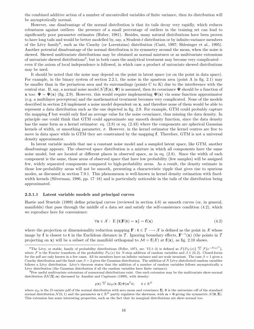
It should be noted that the noise may depend on the point in latent space (or on the point in data space).For example, in the binary system of section 2.2.1, the noise in the apastron area (point A in fig. 2.1) maybe smaller than in the periastron area and its surroundings (points C to K) due to the interference with thecentral star. If, say, a normal noise model N (f(x),Ψ) is assumed, then its covariance Ψ should be a function ofx too: Ψ = Ψ(x) (fig. 2.9). However, this would require implementing Ψ(x) via some function approximator(e.g. a multilayer perceptron) and the mathematical treatment becomes very complicated. None of the modelsdescribed in section 2.6 implement a noise model dependent on x, and therefore none of them would be able torepresent a data distribution such as the one depicted in fig. 2.9. For example, GTM could probably capturethe mapping f but would only find an average value for the noise covariance, thus missing the data density. Inprinciple one could think that GTM could approximate any smooth density function, since the data densityhas the same form as a kernel estimator: eq. (2.8) or eq. (2.43) where the components are spherical Gaussiankernels of width, or smoothing parameter, σ. However, in the kernel estimator the kernel centres are free tomove in data space while in GTM they are constrained by the mapping f . Therefore, GTM is not a universaldensity approximator.

In latent variable models that use a constant noise model and a sampled latent space, like GTM, anotherdisadvantage appears. The observed space distribution is a mixture in which all components have the samenoise model, but are located at different places in observed space, as in eq. (2.8). Since the width of eachcomponent is the same, those areas of observed space that have low probability (few samples) will be assignedfew, widely separated components compared to high-probability areas. As a result, the density estimate inthose low-probability areas will not be smooth, presenting a characteristic ripple that gives rise to spuriousmodes, as discussed in section 7.9.1. This phenomenon is well-known in kernel density estimation with fixed-width kernels (Silverman, 1986, pp. 17–18) and is particularly noticeable in the tails of the distribution beingapproximated.

2.3.1.1 Latent variable models and principal curves

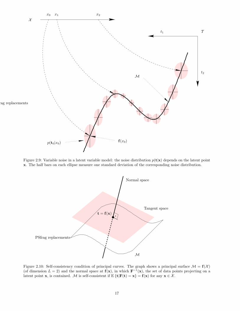
Hastie and Stuetzle (1989) define principal curves (reviewed in section 4.8) as smooth curves (or, in general,manifolds) that pass through the middle of a data set and satisfy the self-consistence condition (4.2), whichwe reproduce here for convenience:

∀x ∈ X : E {t|F(t) = x} = f(x) (4.2)

where the projection or dimensionality reduction mapping F : t ∈ T −→ X is defined as the point in X whoseimage by f is closest to t in the Euclidean distance in T . Ignoring boundary effects, F−1(x) (the points in Tprojecting on x) will be a subset of the manifold orthogonal to M = f(X ) at f(x), as fig. 2.10 shows.

8The Levy, or stable, family of probability distributions (Feller, 1971, sec. VI.1–3) is defined as F{PN (x)} def= F{e−N|x|β},

where F is the Fourier transform of the probability PN (x) for N-step addition of random variables and β ∈ (0, 2). Closed-formsfor the pdf are only known in a few cases. All its members have an infinite variance and are scale invariant. The case β = 1 gives aCauchy distribution and the limit case β = 2 gives the Gaussian distribution. The addition of N Levy-distributed random variablesfollows a Levy distribution. Levy’s theorem states that the addition of a number of random variables follows asymptotically aLevy distribution (the Gaussian distribution if all the random variables have finite variance).

9Few useful multivariate extensions of nonnormal distributions exist. One such extension may be the multivariate skew-normaldistribution SN (Σ, α) discussed by Azzalini and Capitanio (1999), with density:

p(t)def= 2φD(t;Σ)Φ(αT t) t ∈ R

D

where φD is the D-variate pdf of the normal distribution with zero mean and covariance Σ, Φ is the univariate cdf of the standardnormal distribution N (0, 1) and the parameter α ∈ RD partly regulates the skewness, with α = 0 giving the symmetric N (0,Σ).This extension has some interesting properties, such as the fact that its marginal distributions are skew-normal too.

16

PSfrag replacements

t1

t2

T

f(x0)p(t0|x0)

M

Xx0 x1 x2

Figure 2.9: Variable noise in a latent variable model: the noise distribution p(t|x) depends on the latent pointx. The half bars on each ellipse measure one standard deviation of the corresponding noise distribution.

PSfrag replacements

t = f(x)

M

Normal space

Tangent space

Figure 2.10: Self-consistency condition of principal curves. The graph shows a principal surface M = f(X )(of dimension L = 2) and the normal space at f(x), in which F−1(x), the set of data points projecting on alatent point x, is contained. M is self-consistent if E {t|F(t) = x} = f(x) for any x ∈ X .

17

We can see that the principal curve self-consistency condition (4.2) is more restrictive than condition (2.5)(verified by unbiased latent variable models) in that the expectation is restricted to the set F−1(x) rather thanto the whole data space T . In other words, the (unbiased) latent variable model condition (2.5) means thatp(t|x) is centred at f(x) for any x ∈ X , whereas the principal curves self-consistency condition (4.2) meansthat p(t|x) restricted to the points in T projecting onto x (which is a subset of the normal hyperplane to Mat f(x)) is centred at f(x) for any x ∈ X .

Clearly then, redefining self-consistency as condition (2.5) and considering both t and x as random variablesturns the principal curve into a latent variable model. This is what Tibshirani (1992) did, seeking to eliminatethe bias intrinsic to the standard definition of principal curves. He then approached the estimation problemas nonparametric estimation of a continuous mixture (section 2.5.2) and, by assuming a diagonal normaldistribution for p(t|f(x)), reduced it to EM estimation of a Gaussian mixture. As mentioned in section 2.5.2,this has the disadvantage of defining the principal curve f only through a finite collection of points in X ratherthan as a smooth function defined for all points in X .

Under a generative view, such as that adopted for latent variable models (section 2.3), the self-consistencycondition (4.2) is unnatural, since it means that for a point that has been generated in latent space and mappedonto a data space point t, the error added to t must be “clever” enough to perturb the point t in a directionorthogonal to the manifold M at t and do so with mean zero! This only seems possible in the trivial casewhere the tangent manifold is constant in direction, i.e., the principal curve has curvature zero. This is thecase of the principal component subspaces and normal distributions, in which case latent variable models andprincipal curves coincide.

2.3.2 Prior distribution in latent space: interpretability

Given any prior distribution px(x) of the L latent variables x, it is always possible to find an invertibletransformation g to an alternative set of L latent variables y = (y1, . . . , yL) = g(x) having another desireddistribution py(y):

X g−→ Y f ′−→ Tf

The mapping from the new latent space onto the data space becomes f ′ = f ◦g−1, i.e., t = f(x) = f(g−1(y)) =

f ′(y) and the new prior distribution of the y variables becomes py = px |Jg|−1, where Jg

def=(∂gl

∂xk

)

is the

Jacobian of the transformation g. That is, given a space X with a distribution px, to transform it into a spaceY with a distribution py we apply10 an invertible mapping g : X → Y of Jacobian |Jg| = px

py. For example, if

x are independently and normally distributed, transforming yl = exl for l = 1, . . . , L means that yl follow alog-normal distribution.

Thus, fixing the functional form of the prior distribution in latent space is a convention rather than anassumption11. However, doing so requires being able to select f and pd(t|x) from a broad class of functions sothat eq. (2.3) still holds. GTM (section 2.6.5) is a good example: while it keeps the prior p(x) simple (discreteuniform), its mapping f is a generalised linear model (which has universal approximation capabilities).

In particular, we can choose the latent variables to be independent12 and identically distributed, px(x)def=

∏Ll=1 p(xl). Unfortunately, while this is a particularly simple and symmetric choice for prior distribution in

latent space, it does not necessarily simplify the calculation of the difficult L-dimensional integral (2.3), whichis a major shortcoming of the latent variable modelling framework (see section 2.4).

We coincide with Bartholomew (1985) that the latent variables must be seen as constructs designed tosimplify and summarise the observed variables, without having to look for an interpretation for them (whichmay exist in some cases anyway): all possible combinations of p(x) and p(t|x) are equally valid as long as theysatisfy eq. (2.3). Thus, we do not need to go into the issue of the interpretation of the latent variables, whichhas plagued the statistical literature for a very long time without reaching a general consensus.

Another issue is the topology of the true data manifold. For the one-dimensional example of figure 2.13,the data manifold is a closed curve (an ellipse). Thus, modelling it with a latent space that has the topologyof an open curve (e.g. an interval of the Cartesian coordinate x) will lead to a discontinuity where both ends of

10Unfortunately, this is terribly complicated in practice, since solving the nonlinear system of partial differential equations∣∣∣

∂y

∂x

∣∣∣ = px

pyto obtain y = g(x) will be impossible except in very simple cases.

11The choice of a prior distribution in the latent space is completely different from, and much simpler than, the well-knownproblem of Bayesian analysis of choosing a noninformative prior distribution for the parameters of a model (mentioned in sec-tion 6.2.3.2)

12When g is linear and y1, . . . , yL are independent, this is exactly the objective of independent component analysis (section 2.6.3).

18

the curve join: it is impossible to have a continuous mapping between spaces with different topological charac-teristics without having singularities, e.g. mapping a circle onto a line. A representation using a periodic latentvariable is required13 (e.g. the polar angle θ). Although some techniques exist for Gaussian mixture modellingof periodic variables (Bishop and Nabney, 1996), all the latent variable models considered in section 2.6 assumenon-periodic latent variables.

A flexible and powerful representation of the prior distribution can be obtained with a mixture:

p(x)def=

M∑

m=1

p(m)p(x|m)

which keeps the marginalisation in data space (2.3) analytically tractable (if the component marginals are):

p(t) =

∫

Xp(t|x)p(x) dx =

M∑

m=1

p(m)

∫

Xp(t|x)p(x|m) dx. (2.6)

By making the latent space distribution more complex we can have a simpler mapping f . The independentfactor analysis model of Attias (1999), discussed in section 2.6.4, uses this idea, where p(x) is a product ofGaussian mixtures, the mapping is linear and the noise model is normal.

2.3.3 Smooth mapping from latent onto data space: preservation of topographicstructure

In section 2.3 we required the mapping f : X → T to be smooth, that is, continuous and differentiable. Thereare two reasons for this:

• Continuity: this, by definition, will guarantee that points which lie close to each other in the latentspace will be mapped onto points which will be close to each other in data space. In the context ofKohonen maps and similar algorithms for dimensionality reduction this is called topology or topographypreservation (although quantifying this topography preservation is difficult; Bauer and Pawelzik, 1992;Martinetz and Schulten, 1994; Kohonen, 1995; Bezdek and Pal, 1995; Goodhill and Sejnowski, 1997;Villmann et al., 1997; Bauer et al., 1999). It expresses the essential requirement that a continuoustrajectory followed by a point in latent space will generate a continuous trajectory in data space (withoutabrupt jumps). The question of whether the dimensionality reduction mapping from data space ontolatent space is continuous will be dealt with in section 2.9.2.

• (Piecewise) differentiability: this is more of a practical requirement in order to be able to use derivative-based optimisation methods, such as gradient descent.

The more general the class of functions from which we can pick f is (expressed through its parameters), themore flexible the latent variable model is (in that more data space distributions p(t) can be constructed fora given prior p(x), eq. (2.3)), but also the more complex the mathematical treatment becomes and the morelocal optima appear. The quality of the local optima found for models which are very flexible can be dreadful,as that shown in fig. 2.13 for GTM. The problem of local optima is very serious since it affects all localoptimisation methods, i.e., methods that start somewhere in parameter space and move towards a nearbyoptimum, such as the EM algorithm and gradient or Newton methods. The only way for such methods to finda good optimum is to start them from many different locations, but this really does not guarantee any goodresults.

In section 2.3 we also required the mapping f to be nonsingular (as defined in section 2.2.2). This is toensure that the manifold M = f(X ) has the same dimension as the latent space X ; otherwise we would bewasting latent variables.

2.4 The problem of the marginalisation in high dimensions

The latent variable framework is very general, accomodating arbitrary mappings and probability distributions.However, this presents insurmountable mathematical and computational difficulties—particularly in the ana-lytical evaluation of integral (2.3) but also when maximising the log-likelihood (2.9)—so that the actual choice

13It is not enough that a curve self-intersects, as it nearly happens in plot A of fig. 2.13: the almost coincident end points f(x1)and f(xK) of the model manifold correspond to the widely separated end latent grid points x1 and xK .

19

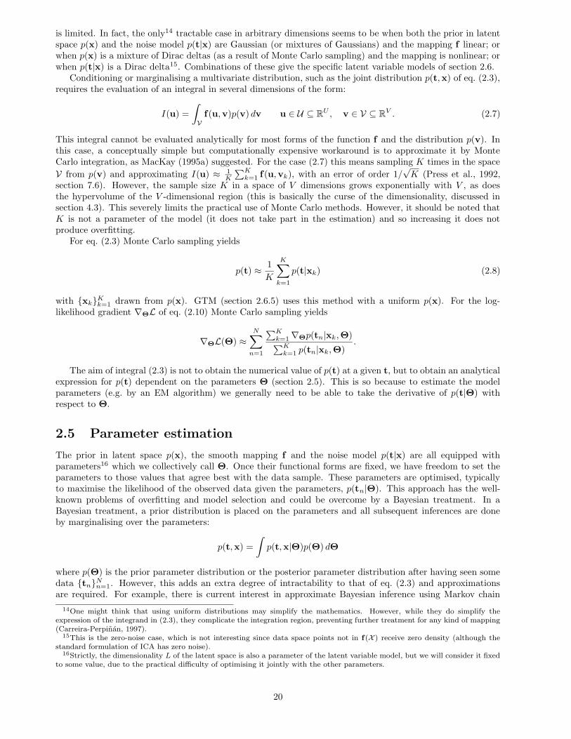
is limited. In fact, the only14 tractable case in arbitrary dimensions seems to be when both the prior in latentspace p(x) and the noise model p(t|x) are Gaussian (or mixtures of Gaussians) and the mapping f linear; orwhen p(x) is a mixture of Dirac deltas (as a result of Monte Carlo sampling) and the mapping is nonlinear; orwhen p(t|x) is a Dirac delta15. Combinations of these give the specific latent variable models of section 2.6.

Conditioning or marginalising a multivariate distribution, such as the joint distribution p(t,x) of eq. (2.3),requires the evaluation of an integral in several dimensions of the form:

I(u) =

∫

Vf(u,v)p(v) dv u ∈ U ⊆ RU , v ∈ V ⊆ RV . (2.7)

This integral cannot be evaluated analytically for most forms of the function f and the distribution p(v). Inthis case, a conceptually simple but computationally expensive workaround is to approximate it by MonteCarlo integration, as MacKay (1995a) suggested. For the case (2.7) this means sampling K times in the space

V from p(v) and approximating I(u) ≈ 1K

∑Kk=1 f(u,vk), with an error of order 1/

√K (Press et al., 1992,

section 7.6). However, the sample size K in a space of V dimensions grows exponentially with V , as doesthe hypervolume of the V -dimensional region (this is basically the curse of the dimensionality, discussed insection 4.3). This severely limits the practical use of Monte Carlo methods. However, it should be noted thatK is not a parameter of the model (it does not take part in the estimation) and so increasing it does notproduce overfitting.

For eq. (2.3) Monte Carlo sampling yields

p(t) ≈ 1

K

K∑

k=1

p(t|xk) (2.8)

with {xk}Kk=1 drawn from p(x). GTM (section 2.6.5) uses this method with a uniform p(x). For the log-likelihood gradient ∇ΘL of eq. (2.10) Monte Carlo sampling yields

∇ΘL(Θ) ≈N∑

n=1

∑Kk=1∇Θp(tn|xk,Θ)∑Kk=1 p(tn|xk,Θ)

.

The aim of integral (2.3) is not to obtain the numerical value of p(t) at a given t, but to obtain an analyticalexpression for p(t) dependent on the parameters Θ (section 2.5). This is so because to estimate the modelparameters (e.g. by an EM algorithm) we generally need to be able to take the derivative of p(t|Θ) withrespect to Θ.

2.5 Parameter estimation

The prior in latent space p(x), the smooth mapping f and the noise model p(t|x) are all equipped withparameters16 which we collectively call Θ. Once their functional forms are fixed, we have freedom to set theparameters to those values that agree best with the data sample. These parameters are optimised, typicallyto maximise the likelihood of the observed data given the parameters, p(tn|Θ). This approach has the well-known problems of overfitting and model selection and could be overcome by a Bayesian treatment. In aBayesian treatment, a prior distribution is placed on the parameters and all subsequent inferences are doneby marginalising over the parameters:

p(t,x) =

∫

p(t,x|Θ)p(Θ) dΘ

where p(Θ) is the prior parameter distribution or the posterior parameter distribution after having seen somedata {tn}Nn=1. However, this adds an extra degree of intractability to that of eq. (2.3) and approximationsare required. For example, there is current interest in approximate Bayesian inference using Markov chain

14One might think that using uniform distributions may simplify the mathematics. However, while they do simplify theexpression of the integrand in (2.3), they complicate the integration region, preventing further treatment for any kind of mapping(Carreira-Perpinan, 1997).

15This is the zero-noise case, which is not interesting since data space points not in f(X ) receive zero density (although thestandard formulation of ICA has zero noise).

16Strictly, the dimensionality L of the latent space is also a parameter of the latent variable model, but we will consider it fixedto some value, due to the practical difficulty of optimising it jointly with the other parameters.

20

Monte Carlo methods (Besag and Green, 1993; Brooks, 1998; Gilks et al., 1996; Neal, 1993) and variationalmethods (Jordan et al., 1999), and this has been applied to some latent variable models, such as principalcomponent analysis (Bishop, 1999) and mixtures of factor analysers (Ghahramani and Beal, 2000; Utsugi andKumagai, 2001). However, these are still preliminary results and the potential gain of using the Bayesiantreatment (notably the autodetection of the optimal number of latent variables and mixture components) maynot warrant the enormous complication of the computations, at least in high dimensions. In this thesis we willonly consider maximum likelihood estimation unless indicated otherwise.

The log-likelihood of the parameters given the sample {tn}Nn=1 is (assuming t1, . . . , tN independent andidentically distributed random variables):

L(Θ)def= ln p(t1, . . . , tN |Θ) = ln

N∏

n=1

p(tn|Θ) =

N∑

n=1

ln p(tn|Θ) (2.9)

which is to be maximised under the maximum likelihood criterion for parameter estimation. This will providewith a set of values for the parameters, Θ∗ = arg maxΘ L(Θ), corresponding to a (local) maximum of thelog-likelihood. The log-likelihood value L(Θ∗) allows the comparison of any two latent variable models (or,in general, any two probability models), however different these may be (although from a Bayesian point ofview, in addition to their likelihood, one should take into account a prior distribution for the parameters andthe evidence for the model; MacKay, 1995b).

One maximisation strategy is to find the stationary points of the log-likelihood (2.9):

∇ΘL(Θ) =N∑

n=1

1

p(tn|Θ)∇Θp(tn|Θ) = 0 (2.10)

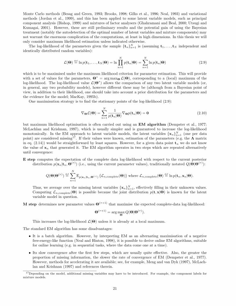
but maximum likelihood optimisation is often carried out using an EM algorithm (Dempster et al., 1977;McLachlan and Krishnan, 1997), which is usually simpler and is guaranteed to increase the log-likelihoodmonotonically. In the EM approach to latent variable models, the latent variables {xn}Nn=1 (one per datapoint) are considered missing17. If their values were known, estimation of the parameters (e.g. the Λ matrixin eq. (2.14)) would be straightforward by least squares. However, for a given data point tn we do not knowthe value of xn that generated it. The EM algorithm operates in two steps which are repeated alternativelyuntil convergence:

E step computes the expectation of the complete data log-likelihood with respect to the current posteriordistribution p(xn|tn,Θ(τ)) (i.e., using the current parameter values), traditionally notated Q(Θ|Θ(τ)):

Q(Θ|Θ(τ))def=

N∑

n=1

Ep(xn|tn,Θ(τ)) {Ln,complete(Θ)} where Ln,complete(Θ)def= ln p(tn,xn|Θ).

Thus, we average over the missing latent variables {xn}Nn=1, effectively filling in their unknown values.Computing Ln,complete(Θ) is possible because the joint distribution p(t,x|Θ) is known for the latentvariable model in question.

M step determines new parameter values Θ(τ+1) that maximise the expected complete-data log-likelihood:

Θ(τ+1) = arg maxΘ

Q(Θ|Θ(τ)).

This increases the log-likelihood L(Θ) unless it is already at a local maximum.

The standard EM algorithm has some disadvantages:

• It is a batch algorithm. However, by interpreting EM as an alternating maximisation of a negativefree-energy-like function (Neal and Hinton, 1998), it is possible to derive online EM algorithms, suitablefor online learning (e.g. in sequential tasks, where the data come one at a time).

• Its slow convergence after the first few steps, which are usually quite effective. Also, the greater theproportion of missing information, the slower the rate of convergence of EM (Dempster et al., 1977).However, methods for accelerating it are available; see, for example, Meng and van Dyk (1997), McLach-lan and Krishnan (1997) and references therein.

17Depending on the model, additional missing variables may have to be introduced. For example, the component labels formixture models.

21

Despite these shortcomings, EM usually remains the best choice for parameter estimation thanks to its relia-bility.

For a general choice of prior in latent space, mapping between latent and data space and noise model thelog-likelihood surface can have many local maxima of varying height. In some cases, some or all of thosemaxima are equivalent, in the sense that the model produces the same distribution (and therefore the samelog-likelihood value at all the maxima), i.e., the model is not identifiable (section 2.8). This is often due tosymmetries of the parameter space, such as permutations (e.g. PCA) or general rotations of the parameters(e.g. factor analysis). In those cases, the procedure to follow is to find a first maximum likelihood estimate ofthe parameters (in general, by some suitable optimisation method, e.g. EM, although sometimes an analyticalsolution is available, as for PCA) and then possibly apply a transformation to them to take them to a canonicalform satisfying a certain criterion (e.g. varimax rotation in factor analysis).

2.5.1 Relation of maximum likelihood with other estimation criteria

Least squares Using the least-squares reconstruction error as objective function for parameter estimationgives in general different estimates as the maximum likelihood criterion, although the latter usually resultsin a low reconstruction error. If we consider the unobserved values {xn}Nn=1 as fixed parameters rather thanrandom variables and assume that the noise model is normal with isotropic known variance, then a penalisedmaximum likelihood criterion results in

N∑

n=1

‖tn − f(xn)‖2 + penalty term on f

which coincides with the spline-related definition of principal curves given by Hastie and Stuetzle (1989),mentioned in section 4.8.

Kullback-Leibler distance For N →∞, the normalised log-likelihood of Θ converges in probability to itsexpectation by the law of large numbers:

LN (Θ)def=

1

N

N∑

n=1

ln p(tn|Θ)P−→ L∞(Θ)

def= Ept {ln p(t|Θ)}

=

∫

Tpt(t) ln p(t|Θ) dt = −h(pt)−D(pt‖p(·|Θ))

(2.11)

for any Θ. Since the entropy of the data distribution h(pt) does not depend on the parameters Θ, maximisingthe log-likelihood is asymptotically equivalent to minimising the Kullback-Leibler distance to the data density.

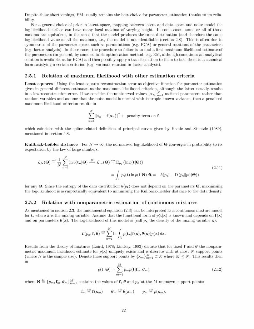
2.5.2 Relation with nonparametric estimation of continuous mixtures

As mentioned in section 2.3, the fundamental equation (2.3) can be interpreted as a continuous mixture modelfor t, where x is the mixing variable. Assume that the functional form of p(t|x) is known and depends on f(x)and on parameters θ(x). The log-likelihood of this model is (call px the density of the mixing variable x):

L(px, f ,θ)def=

N∑

n=1

ln

∫

Xp(tn|f(x),θ(x))p(x) dx.

Results from the theory of mixtures (Laird, 1978; Lindsay, 1983) dictate that for fixed f and θ the nonpara-metric maximum likelihood estimate for p(x) uniquely exists and is discrete with at most N support points(where N is the sample size). Denote these support points by {xm}Mm=1 ⊂ X where M ≤ N . This results thenin

p(t;Θ) =M∑

m=1

pmp(t|fm,θm) (2.12)

where Θdef= {pm, fm,θm}Mm=1 contains the values of f , θ and px at the M unknown support points:

fmdef= f(xm) θm

def= θ(xm) pm

def= p(xm).

22

ModelPrior in latent

space p(x)Mapping f

x→ tNoise model

p(t|x)Density in observed

space p(t)

Factor analysis (FA) N (0, I) lineardiagonalnormal

constrainedGaussian

Principal componentanalysis (PCA)

N (0, I) linearsphericalnormal

constrainedGaussian

Independent componentanalysis (ICA)

unknownbut factorised

linear Dirac delta depends

Independent factoranalysis (IFA)

product of 1DGaussian mixtures

linear normalconstrained

Gaussian mixtureGenerative topographicmapping (GTM)

discreteuniform

generalisedlinear model

sphericalnormal

constrainedGaussian mixture

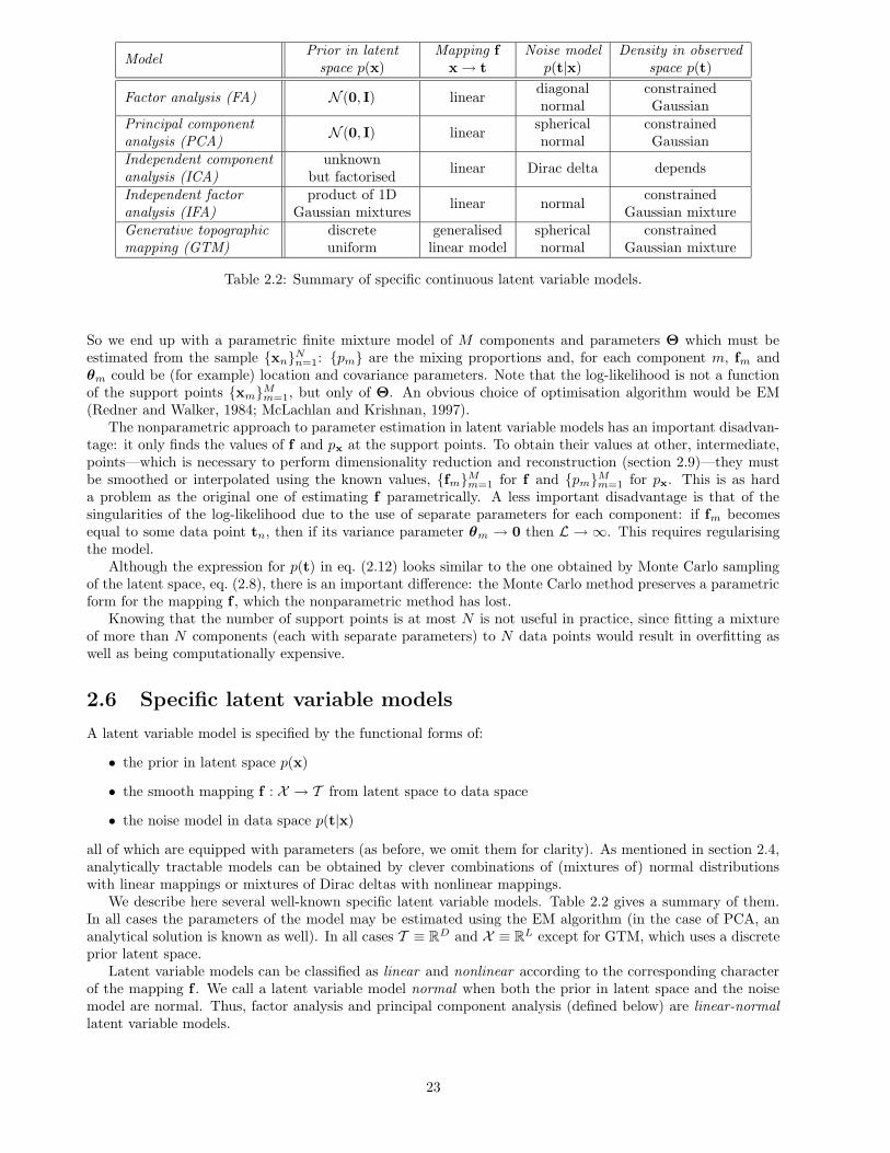
Table 2.2: Summary of specific continuous latent variable models.

So we end up with a parametric finite mixture model of M components and parameters Θ which must beestimated from the sample {xn}Nn=1: {pm} are the mixing proportions and, for each component m, fm andθm could be (for example) location and covariance parameters. Note that the log-likelihood is not a functionof the support points {xm}Mm=1, but only of Θ. An obvious choice of optimisation algorithm would be EM(Redner and Walker, 1984; McLachlan and Krishnan, 1997).

The nonparametric approach to parameter estimation in latent variable models has an important disadvan-tage: it only finds the values of f and px at the support points. To obtain their values at other, intermediate,points—which is necessary to perform dimensionality reduction and reconstruction (section 2.9)—they mustbe smoothed or interpolated using the known values, {fm}Mm=1 for f and {pm}Mm=1 for px. This is as harda problem as the original one of estimating f parametrically. A less important disadvantage is that of thesingularities of the log-likelihood due to the use of separate parameters for each component: if fm becomesequal to some data point tn, then if its variance parameter θm → 0 then L → ∞. This requires regularisingthe model.

Although the expression for p(t) in eq. (2.12) looks similar to the one obtained by Monte Carlo samplingof the latent space, eq. (2.8), there is an important difference: the Monte Carlo method preserves a parametricform for the mapping f , which the nonparametric method has lost.

Knowing that the number of support points is at most N is not useful in practice, since fitting a mixtureof more than N components (each with separate parameters) to N data points would result in overfitting aswell as being computationally expensive.

2.6 Specific latent variable models

A latent variable model is specified by the functional forms of:

• the prior in latent space p(x)

• the smooth mapping f : X → T from latent space to data space

• the noise model in data space p(t|x)

all of which are equipped with parameters (as before, we omit them for clarity). As mentioned in section 2.4,analytically tractable models can be obtained by clever combinations of (mixtures of) normal distributionswith linear mappings or mixtures of Dirac deltas with nonlinear mappings.

We describe here several well-known specific latent variable models. Table 2.2 gives a summary of them.In all cases the parameters of the model may be estimated using the EM algorithm (in the case of PCA, ananalytical solution is known as well). In all cases T ≡ RD and X ≡ RL except for GTM, which uses a discreteprior latent space.

Latent variable models can be classified as linear and nonlinear according to the corresponding characterof the mapping f . We call a latent variable model normal when both the prior in latent space and the noisemodel are normal. Thus, factor analysis and principal component analysis (defined below) are linear-normallatent variable models.

23

2.6.1 Factor analysis (FA)

Factor analysis18 (Bartholomew, 1987; Everitt, 1984) uses a Gaussian distributed prior and noise model, anda linear mapping from data space to latent space. Specifically:

• The latent space prior p(x) is unit normal:

xdef∼ N (0, I) (2.13)

although there exist varieties of factor analysis where these factors are correlated. The latent variablesx are often referred to as the factors.

• The mapping f is linear:

f(x)def= Λx + µ. (2.14)

The columns of the D×L matrix Λ are referred to as the factor loadings. We assume rank (Λ) = L, i.e.,linearly independent factors.

• The data space noise model is normal centred at f(x) with diagonal covariance matrix Ψ:

t|x def∼ N (f(x),Ψ). (2.15)

The D diagonal elements of Ψ are referred to as the uniquenesses.

The marginal distribution in data space can be computed analytically and it turns out to be normal with aconstrained covariance matrix (theorems 2.12.1 and A.3.1(iv)):

t ∼ N (µ,ΛΛT + Ψ). (2.16)

The posterior in latent space is also normal:

x|t ∼ N(

A(t− µ), (I + ΛTΨ−1Λ)−1)

(2.17)

A = ΛT (ΛΛT + Ψ)−1 = (I + ΛTΨ−1Λ)−1ΛTΨ−1. (2.18)

The reduced-dimension representative (defined in section 2.9.1) is taken as the posterior mean (coinciding withthe mode) and is usually referred to as the Thomson scores:

F(t)def= E {x|t} = A(t− µ). (2.19)

The dimensionality reduction mapping F is linear and therefore smooth. As discussed in section 2.9.1.1, factoranalysis with Thomson scores does not satisfy the condition that F◦ f be the identity, because AΛ 6= I, exceptin the zero-noise limit.

If we apply an invertible linear transformation g with matrix R to the factors x to obtain a new set offactors y = Rx, the prior distribution p(y) is still normal (theorem A.3.1(i)), y ∼ N (0,RRT ), and the newmapping becomes t = f ′(y) = f(g−1(y)) = ΛR−1y + µ (section 2.3.2). That is, the new factor loadingsbecome Λ′ = ΛR−1. If R is an orthogonal matrix, i.e., R−1 = RT , the new factors y will still be independentand Ψ′ = Ψ diagonal; this is called an orthogonal rotation of the factors in the literature of factor analysis.If R is an arbitrary nonsingular matrix, the new factors y will not be independent anymore; this is calledan oblique rotation of the factors. Thus, from all the factor loadings matrices Λ, we are free to choose thatwhich is easiest to interpret according to some criterion, e.g. by varimax rotation19. However, we insist that,provided that the model p(t) remains the same, all transformations—orthogonal or oblique—are equally valid.Section 2.8.1 further discusses this issue.

The log-likelihood of the parameters20 Θ = {Λ,Ψ,µ} is obtained as the log-likelihood of a normal distri-bution N (µ,Σ) of covariance Σ = ΛΛT + Ψ:

L(Λ,Ψ) = −N2

(D ln 2π + ln |Σ|+ tr

(SΣ−1

))(2.20)

18Our Matlab implementation of factor analysis (EM algorithm, Rao’s algorithm, scores, χ2-test, etc.) and varimax rotation isfreely available in the Internet (see appendix C).

19Varimax rotation (Kaiser, 1958) finds an orthogonal rotation of the factors such that, for each new factor, the loadings areeither very large or very small (in absolute value). The resulting rotated matrix Λ′ has many values clamped to (almost) 0, thatis, each factor involves only a few of the original variables. This simplifies factor interpretation.

20The maximum likelihood estimate of the location parameter µ is the sample mean t. If the covariance matrix of p(t) ineq. (2.16) was unconstrained, the problem would be that of fitting a normal distribution N (µ,Σ) to the sample {tn}N

n=1. In thiscase, the maximum likelihood estimates for µ and Σ would be the natural ones: the sample mean t and the sample covariancematrix S, respectively (Mardia et al., 1979).

24

where Sdef= 1

N

∑Nn=1 (tn − t)(tn − t)T is the sample covariance matrix and t

def= 1

N

∑Nn=1 tn the sample mean.

The log-likelihood gradient is:

∂L∂Λ

= −N(Σ−1(I− SΣ−1)Λ)∂L∂Ψ

= −N2

diag(Σ−1(I− SΣ−1)

).

The log-likelihood has infinite equivalent maxima resulting from orthogonal rotation of the factors. Apartfrom these, it is not clear whether the log-likelihood has a unique global maximum or there exist suboptimalones. In theory, different local maxima are possible and should be due to an underconstrained model (e.g. asmall sample), but there does not seem to be any evidence in the factor analysis literature about the frequencyof multiple local maxima with actual data. Rubin and Thayer (1982), Bentler and Tanaka (1983) and Rubinand Thayer (1983) give an interesting discussion about this21.

The parameters of a factor analysis model may be estimated using an EM algorithm (Rubin and Thayer,1982):

E step: This requires computing the moments:

E {x|tn} = A(τ)(tn − µ)

E{xxT |tn

}= I−A(τ)Λ(τ) + A(τ)(tn − µ)(tn − µ)T (A(τ))T

for each data point tn given the current parameter values Λ(τ) and Ψ(τ).

M step: This results in the following update equations for the factor loadings Λ and uniquenesses Ψ:

Λ(τ+1) =

(N∑

n=1

tn E {x|tn}T)(

N∑

n=1

E{xxT |tn

}T

)−1

Ψ(τ+1) =1

Ndiag

(N∑

n=1

tn tTn −Λ(τ+1) E{x|tn

}tTn

)

where the updated moments are used and the “diag” operator sets all the off-diagonal elements of amatrix to zero.

The location parameter µ is estimated by the sample mean, and does not need to take part in the EMalgorithm.

Apart from EM, there are a number of other methods for maximum likelihood parameter estimation forfactor analysis, such as the methods of Joreskog (1967)22 or Rao (Morrison, 1990, pp. 357–362). Also, incommon with other probabilistic models, factor analysis may be implemented using an autoencoder network,with weights implementing a recognition and a generative model: a special case of the Helmholtz machinehaving two layers of linear units with Gaussian noise, and trained with the wake-sleep algorithm23 (Neal andDayan, 1997).

There are also estimation criteria for factor analysis other than maximum likelihood, e.g. principal factors(Harman, 1967) or minimum trace factor analysis (Jamshidian and Bentler, 1998).

2.6.2 Principal component analysis (PCA)

Principal component analysis24 (PCA) can be seen as a maximum likelihood factor analysis in which theuniquenesses are constrained to be equal, that is, Ψ = σ2I is isotropic. This simple fact, already reportedin the early factor analysis literature, seems to have gone unnoticed until Tipping and Bishop (1999b) andRoweis (1998) recently rediscovered it. Indeed, a number of textbooks and papers (e.g. Krzanowski, 1988,

21Rubin and Thayer (1982), reanalysing an example with 9 observed variables, 4 factors and around 36 free parameters in whichJoreskog had found a single maximum with the LISREL method, claimed to find several additional maxima of the log-likelihoodusing their EM algorithm. By carefully checking the gradient and the Hessian of the log-likelihood at those points, Bentlerand Tanaka (1983) showed that none except Joreskog’s were really maxima. This is disquieting in view of the large number ofparameters used in pattern recognition applications.

22The method of Joreskog (1967) is a second-order Fletcher-Powell method. It is also applicable to confirmatory factor analysis,where some of the loadings have been set to fixed values (usually zero) according to the judgement of the user (Joreskog, 1969).

23Strictly speaking, Neal and Dayan (1997) give no proof that wake-sleep learning works for factor analysis, only empiricalsupport that it usually does in some simulations.

24Our Matlab implementation of principal component analysis is freely available in the Internet (see appendix C).

25

p. 502 or Hinton et al., 1997, beginning of section III) wrongly quote that “PCA does not propose a model forthe data” as a disadvantage when compared with factor analysis.

The approach of considering an isotropic noise model in factor analysis had already been adopted inthe Young-Whittle factor analysis model (Young, 1940; Whittle, 1952) and its maximum likelihood solutionassuming σ known found analytically (Anderson, 1963; Basilevsky, 1994, pp. 361–363). Lawley (1953) andAnderson and Rubin (1956) showed that stationary points of the log-likelihood as a function of the loadingsΛ and uniqueness σ2 occur at the value of eq. (2.28), although they did not prove it to be global maximum,which Tipping and Bishop (1999b) did. In addition to this direct solution, Roweis (1998) and Tipping andBishop (1999b) give an EM algorithm for estimating Λ and σ2.

Consider then the factor analysis model of the previous section with an isotropic error model. There existsa unique (although possibly degenerate, if some eigenvalues are equal) maximum likelihood estimate closelyrelated to the L principal components of the data25. If the sample covariance matrix is decomposed as S =UVUT , with V = diag (v1, . . . , vD) containing the eigenvalues (ordered decreasingly) and U = (u1, . . . ,uD)the associated eigenvectors, then Λ = UL(VL − σ2I)1/2 with UL = (u1, . . . ,uL), VL = diag (v1, . . . , vL) and

σ2 = 1D−L

∑Dj=L+1 vj . Therefore eqs. (2.13)–(2.19) become:

xdef∼ N (0, I) (2.21)

f(x)def= Λx + µ (2.22)

t|x def∼ N (f(x), σ2I) (2.23)

t ∼ N (µ,ΛΛT + σ2I) (2.24)

x|t ∼ N(A(t− µ), σ2V−1

L

)(2.25)

A = V−1L (VL − σ2I)1/2UT

L (2.26)

F(t)def= E {x|t} = A(t− µ) (2.27)

with maximum likelihood estimates:

Λ = UL(VL − σ2I)1/2 σ2 =1

D − LD∑

j=L+1

vj . (2.28)

The Thomson scores give F(t) = E {x|t} = A(t− µ), which still does not satisfy the condition that F ◦ f bethe identity, except in the zero-noise limit (σ → 0), as discussed in section 2.9.1.1.

Thus, in the latent variable model scenario PCA does define a probability model. Still, PCA is not usuallyconstructed as a probability model but as a reconstruction and dimensionality reduction technique, since itsmost attractive property is that it is the linear mapping that minimises the least squares reconstruction errorof a sample. We describe this aspect of PCA in section 4.5.

Since the noise model variance σ2 is the same for all observed variables, the directions of the columns ofΛ will be more influenced by the variables that have higher noise—unlike with factor analysis, which shouldbe able to separate the linear correlations from the noise. The PCA model is then more restricted than thefactor analysis one. However, in many practical situations the directions Λ found by factor analysis and PCAdo not differ much.

The log-likelihood of the estimate (2.28) is26

L(Λ, σ2) = −N2

(

D(1 + ln 2π) + ln |S|+ (D − L) lna

g

)

(2.29)

where a and g are the arithmetic and geometric means of the D − L smallest eigenvalues of the samplecovariance matrix S. Although there is an EM algorithm that finds the L principal components by maximisingthe log-likelihood (Tipping and Bishop, 1999b; Roweis, 1998), the fastest way to perform PCA is via numericalsingular value decomposition (Golub and van Loan, 1996; Press et al., 1992).

Again, as in factor analysis, it is possible to orthogonally rotate the latent variables keeping the samedistribution.

25To differentiate it from conventional PCA, where no probabilistic model is explicitly defined and only a linear orthogonalprojection is considered (section 4.5), this latent variable model is called probabilistic PCA by Tipping and Bishop (1999b) andsensible PCA by Roweis (1998). We do not deem necessary to use and additional, different name for what is essentially the samething, so in this thesis we will only use the name PCA and the context will make clear what aspect we mean—probability modelor linear mapping.

26As with factor analysis, the maximum likelihood estimate of the location parameter µ is the sample mean t.

26

For a fixed data set, PCA has the property of additivity, insofar that the principal components obtainedusing a latent space of dimension L are exactly the same as the ones obtained using a latent space of dimensionL− 1 plus a new, additional principal component. However, this additivity property does not necessarily holdfor either PCA followed by (varimax) rotation or for factor analysis. That is, the factors found by a factoranalysis of order L are, in general, all different from those found by a factor analysis of order L − 1. Thatmeans that one can only talk about the joint collection of L factors (or the linear subspace spanned by them).

2.6.3 Independent component analysis (ICA)

Independent component analysis (ICA) or blind source separation consists of recovering independent sourcesgiven only sensor observations that are unknown linear mixtures of the sources (Comon, 1994; Cardoso, 1998;Hyvarinen, 1999b; Hyvarinen et al., 2001). Its basic formulation is as follows. Denote the time variable byτ (continuous or discrete). Call x(τ) ∈ RL the L time-varying source signals27, assumed independent andzero-mean. Call t(τ) ∈ RD the D data signals, measured without noise and with instantaneous mixing28 (that

is, there is no time delay between source l mixing into channel d). Then t(τ)def= Λx(τ), where ΛD×L is the

mixing matrix and D ≥ L (although we will assume D = L in most of this section29). The goal of ICA is,given a sample {tn}Nn=1 of the sensor outputs, to find a linear transformation AL×D (separating matrix ) of thesensor signals t that makes the outputs u(τ) = At(τ) = AΛx(τ) as independent as possible. If Λ was known,A = Λ+ = (ΛTΛ)−1ΛT (assuming rank (Λ) = L) would recover the sources exactly, but Λ is unknown; allwe have is a finite set of realisations of the sensor outputs {tn}Nn=1.

If we take the sources x = (x1, . . . , xL)T as the latent variables and the sensor outputs t = (t1, . . . , tD)T asthe observed variables, ICA can be seen as a latent variable model with the following elements (the dependenceon the time τ is omitted for clarity):

• The prior distribution in latent space X = RL is factorised but unknown: p(x) =∏Ll=1 pl(xl).

• The mapping between latent and observed space is linear: t = Λx.

• The noise model is a Dirac delta, i.e., the observed variables are generated without noise: p(t|x) =

δ(t−Λx) =∏Dd=1 δ(td −

∑Ll=1 adlxl). However, we can imagine that noise is an independent source and

segregate it from the other sources.

Therefore, the only free parameter in the latent variable model is the matrix ΛD×L = (λdl) (or AL×D = Λ+ =(ald)), but it is also necessary to determine the unknown functions {pl(xl)}Ll=1. How to deal with this unknownprior distribution is what makes ICA different from the other latent variable models discussed here. Ideally onewould learn the functions {pl}Ll=1 nonparametrically, but this is difficult. For practical estimation, all currentmethods use a fixed functional form for the latent space prior distribution with or without parameters. Aflexible parametric model of the prior distribution is a Gaussian mixture and this gives rise to the IFA modelof section 2.6.4.

The very effective infomax learning rule of Bell and Sejnowski (1995) is the following online iterativealgorithm:

A(τ+1) = A(τ) + ∆A(τ+1) (2.30)

∆A(τ+1) ∝ ((A(τ))T )−1 + g(u)tT (2.31)

where t is a sensor output, udef= A(τ)t, g(u)

def= (g(u1), . . . , g(uL))T and g(u)

def=

∂ ln |f ′(u)|∂u . The choice of the

nonlinear function f : R→ R is critical since it can be proven (see below and Bell and Sejnowski, 1995) thatp(xl) ∝ |f ′(xl)|. That is, f is the one-dimensional cumulative distribution function in latent space and fixingits form is equivalent to assuming a prior distribution p(xl) for the latent variables (the sources). Takingg(u) = −2u (or equivalently f = erf) means assuming normally distributed sources, x ∼ N (0, I) (althoughwith a Dirac-delta noise model), which gives second-order decorrelation only—in which case using factoranalysis would have been enough. The use of a nonlinear function, whose Taylor series expansion has terms ofmany orders, may be more sensitive to the right higher-order statistics of the inputs. In practice, a sigmoidalfunction is chosen, such as the logistic function. Several forms of the nonlinearity f are summarised in table 2.3.The computationally simpler nonlinearities, such as the logistic function or the hyperbolic tangent, assume

27Instead of time-varying sources x(τ) one can consider space-varying sources x(x, y), such as images.28If time delays are considered, the problem is called blind deconvolution rather than blind separation.29The case D < L (more sources than sensors) is called overcomplete representation and has been advocated because of its

greater robustness to noise, sparsity and flexibility in matching structure in the data (Amari, 1999; Lewicki and Sejnowski, 2000).

27

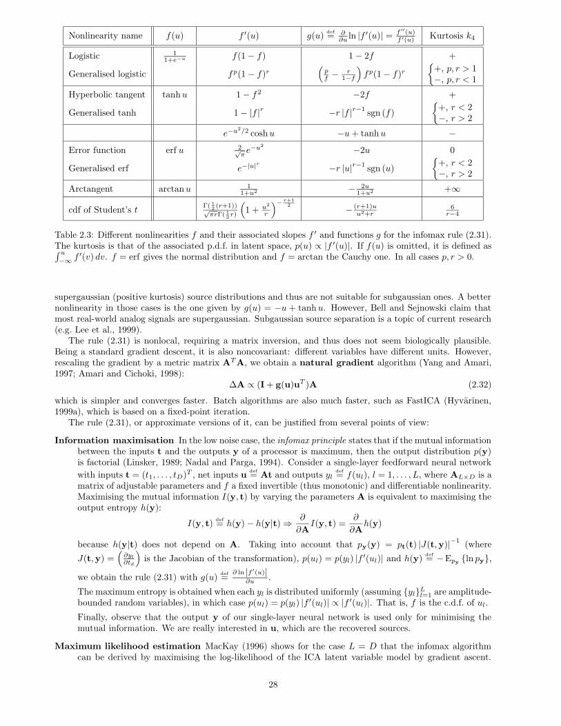
Nonlinearity name f(u) f ′(u) g(u)def= ∂

∂u ln |f ′(u)| = f ′′(u)f ′(u) Kurtosis k4

Logistic 11+e−u f(1− f) 1− 2f +

Generalised logistic fp(1− f)r(pf − r

1−f

)

fp(1− f)r{

+, p, r > 1−, p, r < 1

Hyperbolic tangent tanhu 1− f 2 −2f +

Generalised tanh 1− |f |r −r |f |r−1sgn (f)

{+, r < 2−, r > 2

e−u2/2 coshu −u+ tanhu −

Error function erf u 2√πe−u

2 −2u 0

Generalised erf e−|u|r −r |u|r−1sgn (u)

{+, r < 2−, r > 2

Arctangent arctanu 11+u2 − 2u

1+u2 +∞

cdf of Student’s tΓ( 1

2 (r+1))√πrΓ( 1

2 r)

(

1 + u2

r

)− r+12 − (r+1)u

u2+r6r−4

Table 2.3: Different nonlinearities f and their associated slopes f ′ and functions g for the infomax rule (2.31).The kurtosis is that of the associated p.d.f. in latent space, p(u) ∝ |f ′(u)|. If f(u) is omitted, it is defined as∫ u

−∞ f ′(v) dv. f = erf gives the normal distribution and f = arctan the Cauchy one. In all cases p, r > 0.

supergaussian (positive kurtosis) source distributions and thus are not suitable for subgaussian ones. A betternonlinearity in those cases is the one given by g(u) = −u + tanhu. However, Bell and Sejnowski claim thatmost real-world analog signals are supergaussian. Subgaussian source separation is a topic of current research(e.g. Lee et al., 1999).

The rule (2.31) is nonlocal, requiring a matrix inversion, and thus does not seem biologically plausible.Being a standard gradient descent, it is also noncovariant: different variables have different units. However,rescaling the gradient by a metric matrix ATA, we obtain a natural gradient algorithm (Yang and Amari,1997; Amari and Cichoki, 1998):

∆A ∝ (I + g(u)uT )A (2.32)

which is simpler and converges faster. Batch algorithms are also much faster, such as FastICA (Hyvarinen,1999a), which is based on a fixed-point iteration.

The rule (2.31), or approximate versions of it, can be justified from several points of view:

Information maximisation In the low noise case, the infomax principle states that if the mutual informationbetween the inputs t and the outputs y of a processor is maximum, then the output distribution p(y)is factorial (Linsker, 1989; Nadal and Parga, 1994). Consider a single-layer feedforward neural network

with inputs t = (t1, . . . , tD)T , net inputs udef= At and outputs yl

def= f(ul), l = 1, . . . , L, where AL×D is a

matrix of adjustable parameters and f a fixed invertible (thus monotonic) and differentiable nonlinearity.Maximising the mutual information I(y, t) by varying the parameters A is equivalent to maximising theoutput entropy h(y):

I(y, t)def= h(y)− h(y|t)⇒ ∂

∂AI(y, t) =

∂

∂Ah(y)

because h(y|t) does not depend on A. Taking into account that py(y) = pt(t) |J(t,y)|−1(where

J(t,y) =(∂yl

∂td

)

is the Jacobian of the transformation), p(ul) = p(yl) |f ′(ul)| and h(y)def= −Epy {ln py},

we obtain the rule (2.31) with g(u)def=

∂ ln |f ′(u)|∂u .

The maximum entropy is obtained when each yl is distributed uniformly (assuming {yl}Ll=1 are amplitude-bounded random variables), in which case p(ul) = p(yl) |f ′(ul)| ∝ |f ′(ul)|. That is, f is the c.d.f. of ul.

Finally, observe that the output y of our single-layer neural network is used only for minimising themutual information. We are really interested in u, which are the recovered sources.

Maximum likelihood estimation MacKay (1996) shows for the case L = D that the infomax algorithmcan be derived by maximising the log-likelihood of the ICA latent variable model by gradient ascent.

28

Let us compute the probability distribution induced in the observed space for the particular case L = Dby marginalising the joint distribution as in eq. (2.3):

p(t) =

∫

Xp(t|x)p(x) dx =

∫

Xδ(t−Λx)p(x) dx = |Λ|−1

p(Λ−1t) = |Λ|−1L∏

l=1

pl

(D∑

d=1

λ−1ld td

)

.

So we get:

as a function of Λ: ln p(t|Λ) = − ln |Λ|+L∑

l=1

ln pl

(D∑

d=1

λ−1ld td

)

as a function of A = Λ−1: ln p(t|A) = ln |A|+L∑

l=1

ln pl

(D∑

d=1

aldtd

)

.

Calling udef= At and g(u)

def=(d ln p1(u1)

du1, . . . , d ln pL(uL)

duL

)T

and using the matrix differentiation identi-

ties (A.4) we obtain the gradient of the log-likelihood:

∂

∂λdlln p(t|Λ) = −ald − ul

L∑

l′=1

al′dgl′(ul′)

∂

∂aldln p(t|Λ) = λdl + gl(ul)td

which coincides with the infomax one, eq. (2.31).

An alternative derivation from a maximum likelihood estimation point of view has been given by Pearl-mutter and Parra (1996) and Cardoso (1997). Consider a parametric model pΘ(t) for the true sensordistribution pt(t). Eq. (2.11) shows that maximising the log-likelihood of Θ is equivalent to minimis-ing the Kullback-Leibler distance to the data density pt(t). Assuming A and Λ invertible, and (a)since H(pt) is independent of A and (b) the Kullback-Leibler divergence is invariant under invertibletransformations (t = Λx and u = At), maximum likelihood estimation produces:

∆A ∝ ∂L(Θ)

∂A

(a)= − ∂

∂AD (pt(t)‖pΘ(t))

(b)= − ∂

∂AD(p(x)‖pΘ(u))

which coincides with the infomax rule of eq. (2.31).

Negentropy maximisation and projection pursuit From a projection pursuit point of view (section 4.6),ICA looks for linear projections where the data become independent. Girolami et al. (1998) show thatnegentropy maximisation projection pursuit performs ICA on sub- or supergaussian sources and leadsexactly to the infomax rule (2.31). Negentropy of a distribution of density p is defined as the Kullback-Leibler divergence between p and the Gaussian distribution pN with the same mean and covariance asp: D (p‖pN ). It is zero if p is normal and positive otherwise.

Cumulant expansion If u and x are symmetrically distributed and approximately normal, their mutualinformation can be approximated using a Gram-Charlier or Edgeworth polynomial expansion (Kendalland Stuart, 1977) of fourth order in terms of the cumulants (Comon, 1994) and used as objective functionfor gradient ascent. However, this method requires more computations than the infomax algorithm andgives worse separation—an order higher than 4 is necessary to improve separation.

Nonlinear PCA Karhunen and Joutsensalo (1994) show that a neural network trained by least squares tocompute the function Af(At) on prewhitened data can separate signals. Girolami and Fyfe (1999) showthat its cost function is approximately equivalent to that of the cumulants method.

2.6.4 Independent factor analysis (IFA)

Independent factor analysis (Attias, 1998, 1999) uses a factorial Gaussian mixture prior, a linear mappingfrom data space to latent space and a normal noise model30. Specifically:

30Similar approaches have also been proposed that use mixture models for the source density: Pearlmutter and Parra (1996)(mixture of logistic densities, gradient descent) and Moulines et al. (1997) and Xu et al. (1998) (Gaussian mixture, EM algorithm).

29

• Each latent variable is modelled independently of the others as a mixture of Ml one-dimensional Gaus-sians:

p(x)def=

L∏

l=1

pl(xl) pl(xl)def=

Ml∑

ml=1

p(ml)p(xl|ml) xl|mldef∼ N (µl,ml

, vl,ml). (2.33)

Thus the latent space prior p(x) is a product of one-dimensional Gaussian mixtures, which results in amixture of L-dimensional diagonal Gaussians but with constrained means and covariance matrices (sincea general mixture of diagonal Gaussians need not be factorised):

p(x) =∑

m

p(m)p(x|m)

mdef= (m1, . . . ,mL)

p(m) =∏Ll=1 p(ml)

x|m def∼ N (µm,Vm) with

{

µm

def= (µ1,m1

, . . . , µL,mL)T

Vmdef= diag (v1,m1

, . . . , vL,mL) .

(2.34)

The summation over m includes all combinations of tuples m = (m1, . . . ,mL) where ml = 1, . . . ,Ml foreach l = 1, . . . , L.

• The mapping f is linear (the data space distribution is assumed zero-mean, which can be obtained bycentring the data sample before fitting the model):

f(x)def= Λx. (2.35)

We assume rank (Λ) = L.

• The data space noise model is normal centred at f(x) with covariance matrix Φ:

t|x def∼ N (f(x),Φ). (2.36)

Thus, factor analysis (and PCA) is a particular case of IFA where Φ is diagonal and each pl(xl) is N (0, 1).The marginal distribution in data space can be computed analytically and turns out to be a constrained

mixture of Gaussians (eq. (2.6) and theorems 2.12.1 and A.3.1(iv)):

p(t) =∑

m

p(m)p(t|m) t|m def∼ N (Λµm,ΛVmΛT + Φ). (2.37)

The posterior in latent space is also a mixture of Gaussians:

p(x|t) =∑

m

p(m|t)p(x|m, t)

p(m|t) = p(t|m)p(m)∑

m′ p(t|m′)p(m′)

(x|m, t)def∼ N (νm,t,Σm)

{

Σmdef= (ΛTΦ−1Λ + V−1

m )−1

νm,tdef= Σm(ΛTΦ−1t + V−1

m µm).

(2.38)

The reduced-dimension representative can be taken as the posterior mean, which is simple to compute (and itneed be computed in each iteration of the EM algorithm):

F(t)def= E {x|t} =

∑

m

p(m|t)νm,t. (2.39)

Since the posterior (2.38) can be asymmetric or multimodal, one could take its mode instead (which couldbe computed iteratively with the algorithms of chapter 8). In the limit of zero noise, the reduced-dimensionrepresentative can be taken as the projection via the pseudoinverse Λ+ = (ΛTΛ)−1ΛT , as in ICA.

Attias (1999) gives an EM algorithm for IFA. Taking the limit Φ→ 0 in it results in an EM algorithm forPCA, as presented by Tipping and Bishop (1999b) and Roweis (1998). Attias (1999) also gives an EM and ageneralised EM algorithm for noiseless IFA (Φ = 0). The latter results in a combination of a rule similar tothe infomax rule (2.31) for updating the mixing matrix and update rules for the Gaussian mixture parameterssimilar to those of the standard EM algorithm for a Gaussian mixture. That is, it combines separating thesources x1, . . . , xL with learning their densities.

Again, a major disadvantage of the IFA model is that the number of parameters grows exponentially withthe dimensionality of the latent space: the prior distribution for the latent variables includes

∏Ll=1 (2Ml − 1)

parameters, which is O(eL). Attias (1999) proposes a variational approximation of the EM algorithm thatreduces the number of operations—but the number of parameters remains O(eL).

30

2.6.5 The generative topographic mapping (GTM)

The generative topographic mapping (GTM) (Bishop, Svensen, and Williams, 1998b) is a nonlinear latentvariable model which has been proposed as a principled alternative to self-organising feature maps (Kohonen,1995). Specifically:

• The L-dimensional latent space X is discrete31. The prior in latent space, p(x), is discrete uniform,assigning nonzero probability only to the points {xk}Kk=1 ⊂ RL, usually arranged in a regular grid (forvisualisation purposes):

p(x)def=

1

K

K∑

k=1

δ(x− xk). (2.40)

This discrete prior can be seen as a fixed approximation of a continuous, uniform distribution in ahyperrectagle of RL (see section 2.4 on Monte Carlo sampling).

• The mapping f is a generalised linear model:

f(x)def= Wφ(x), (2.41)

where W is a D × F matrix and φ an F × 1 vector of fixed basis functions.

• The noise model p(t|x) is an isotropic normal centred at f(x):

t|x def∼ N (f(x), σ2I). (2.42)

The marginal distribution in data space is a constrained mixture of Gaussians (in the sense that the Gaussiancentres cannot move independently, but only by changing the mapping f through W):

p(t) =1

K

K∑

k=1

p(t|xk), (2.43)

and the posterior in latent space is discrete:

p(xk|t) =p(t|xk)

∑Ki=1 p(t|xi)

. (2.44)

The reduced-dimension representative can be taken as the posterior mean or the posterior mode, both ofwhich can be easily computed since the posterior distribution is discrete. The mean and the mode can bequite different from each other if the posterior distribution is multimodal. The dimensionality reductionmapping F for the posterior mode is not continuous in general, although it will be approximately continuous ifthe posterior distribution (2.44) is unimodal and sharply peaked for most points in data space (section 2.9.2).

The log-likelihood of the parameters Θ = {W, σ2} is

L(W, σ2) =

N∑

n=1

ln1

K

K∑

k=1

p(tn|xk;W, σ2) =

N∑

n=1

ln1

K(2πσ2)D2

K∑

k=1

e−1

2σ2 ‖tn−Wφ(xk)‖2

and is known to contain a number of suboptimal maxima (see fig. 2.13 for some examples).The parameters of a GTM model may be estimated using the EM algorithm:

E step This requires computing the responsibility Rnk = p(xk|tn) of each latent space point xk havinggenerated point tn using eqs. (2.40)-(2.44) with the current parameter values W(τ) and σ(τ).

M step This results in the following update equations for the parameters W and σ, respectively:

ΦTG(τ)Φ(W(τ+1))T = ΦT (R(τ))TT (2.45a)

(σ(τ+1))2 =1

ND

K∑

k=1

N∑

n=1

R(τ)nk ‖tn − f(xk)‖2 (2.45b)

where Φdef= (φ1, . . . ,φK)T , T

def= (t1, . . . , tN )T , R is an N × K matrix with elements Rnk and G is a

K ×K diagonal matrix with elements gkk =∑Nn=1Rnk. Solving for W requires (pseudo-)inverting the

matrix ΦTGΦ at each iteration.31Strictly, the latent space is continuous and p(x) is a density, but we will call it “discrete uniform” for short (see also sections 2.4

and 2.9.2).

31

A simple regularised version of GTM to control the mapping f is obtained by placing an isotropic Gaussian

prior distribution of variance λ−1 on the mapping weights W = (wdf ), W|λ def∼ N (0, λ−1I). This leads to amaximum a posteriori (MAP) estimator:

LMAP(W, σ2) = L(W, σ2)− Nλ

2‖W‖2 (2.46)

where λ is the regularisation coefficient, ‖W‖2 =∑Dd=1

∑Ff=1 w

2df and an additive term independent of W

and σ2 has been omitted. This results in a modified M step of the EM algorithm:

(ΦTG(τ)Φ + λσ2I)(W(τ+1))T = ΦT (R(τ))TT.

An approximate Bayesian treatment of the hyperparameter λ is given by Bishop et al. (1998a) and Utsugi(2000).

The major shortcoming of GTM is that, being based on (fixed) Monte Carlo sampling of the latent spacementioned in section 2.4, both the number of latent grid points K and the number of basis functions F requiredfor the generalised linear model (2.41) grow exponentially with the dimension of the latent space, L. This limitsthe practical applicability of GTM to about 2 latent variables. Another shortcoming, shared by most globalmethods (i.e., that find an estimate for the whole data space) that are very flexible parameterised models, isthe fact that the EM estimate very often converges to very bad local maxima, as those shown in the lower halfof fig. 2.13; for twisted manifolds, a good maximum can only be reached it starting EM from a small region ofthe parameter space.

The density networks of MacKay (1995a) are a model similar to GTM: the mapping f is implementedby a multilayer perceptron, all the distributions are assumed isotropic Gaussian and a Monte Carlo fixedsampling is necessary to obtain p(t). The log-likelihood is maximised with a conjugate gradients method. LikeGTM, this approach suffers from the exponential complexity of the Monte Carlo sampling. MacKay appliesdensity networks to a discrete problem, modelling a protein family. The insight of (Bishop et al., 1998b) isto implement the mapping f with a generalised linear model, which results in a tractable M step of the EMalgorithm, since only the weights of the linear layer have to be estimated.

GTM pursues a similar goal as Kohonen’s self-organising maps (to adapt a topographical arrangement ofknots to a data distribution) but with the important advantage that it defines a probabilistic model for thedata and dimensionality reduction and reconstruction mappings. Table 4.4 compares succintly both models.

2.6.5.1 Extensions to GTM

Bishop et al. (1998a) propose several extensions to the GTM model:

• A manifold-aligned noise model, where the covariance matrix of the noise model (2.42) is not isotropicanymore but approximately aligned (depending on the value of η below) with the manifold M = f(X )locally at each mapped point f(x):

t|x def∼ N (f(x),Σ(x)) Σ(x)def= σ2I + η

L∑

l=1

∂f

∂xl

(∂f

∂xl

)T

where the new hyperparameter η must be adjusted manually and Σ(x) is computed only at the points{xk}Kk=1. The goal is to ensure that the variance of the noise distribution in directions tangential tothe manifold is never significantly less than the square of the typical distance between neighbouringpoints f(xk), so that there is a smooth distribution along the manifold even when the noise varianceperpendicular to the manifold becomes small.

It would seem that this model violates the axiom of local independence (section 2.3.1), since Σ(x) isnot diagonal and so the noise model would not be factorised anymore. However, the model can bederived from taking the model with factorised axis-aligned noise, but approximating the uniform densityby a grid of Gaussians (rather than deltas) and then linearising the manifold about the centre of eachGaussian (Chris Williams, pers. comm.).

It remains to be seen whether this approach has any advantages over using a mixture of linear-normallatent variable models (since each GTM mixture component represents now a local linear subspace).

• Modelling of discrete observed variables by defining a Bernoulli or multinomial noise model dependingon f(x) via a logistic or softmax function, respectively. However, estimation of the parameters via theEM algorithm is much more difficult, requiring nonlinear optimisation in the M step.

32

• A semilinear model where some of the latent variables are discretised and mapped with the generalisedlinear model (2.41) as in the standard GTM model and the rest are continuous and mapped linearly.

• An incremental EM algorithm based on the approach of Neal and Hinton (1998).

• Approximate Bayesian inference for the regularisation parameter λ of eq. (2.46), using the Laplaceapproximation (MacKay, 1992a), i.e., a local Gaussian approximation at the mode of the posteriordistribution of the parameters W. The Laplace approximation breaks down when the posterior parameterdistribution is multimodal or skewed—a likely situation when training data is scarce (Richardson andGreen, 1997). Utsugi (2000) uses a Gibbs sampler and an ensemble learning method to approximateBayesian inference.

• A Gaussian process formulation.

Further extensions by other authors include:

• Marrs and Webb (1999) propose an average generalised unit-speed constraint on f to preserve geodeticdistances in data space (outlined in section 2.8.3).

• We propose a diagonal noise GTM model (dGTM), where the noise model covariance is diagonal ratherthan spherical: t|x ∼ N (f(x),Ψ) with Ψ = diag (ψ1, . . . , ψD). In section 2.12.4 we show that the EMalgorithm remains the same except for eq. (2.45b), which becomes D equations:

ψ(τ+1)d =

1

N

K∑

k=1

N∑

n=1

R(τ)nk (tnd − fd(xk))2 d = 1, . . . , D (2.45b’)

and the responsibilities Rnk depend on Ψ rather than on σ2.

A diagonal noise model is necessary to account for different scales and noise levels in the different datavariables t1, . . . , tD (which in general cannot be overcome by presphering the data, as fig. 2.8 shows).

2.7 Finite mixtures of latent variable models

Finite mixtures (Everitt and Hand, 1981) of latent variable models can be constructed in the usual way as32

p(t)def=

M∑

m=1

p(m)p(t|m) (2.47)

where:

• p(t|m), m = 1, . . . ,M are latent variable models based on latent spaces Xm of dimension Lm (notnecessarily equal), i.e.,

p(t|m) =

∫

Xm

p(t,x|m) dx =

∫

Xm

p(t|x,m)p(x|m) dx

where p(x|m) is the prior distribution in the latent space of the mth component, p(t|x,m) its noisemodel and fm : Xm → T its mapping from latent space into data space.

• p(m) are the mixing proportions.

The joint density is p(t,x,m) = p(t|x,m)p(x|m)p(m) and the finite mixture distribution can be expressed asthe marginalisation of p(t,x,m) over x and m:

p(t) =

M∑

m=1

∫

Xm

p(t,x,m) dx =

M∑

m=1

p(m)

∫

Xm

p(t|x,m)p(x|m) dx =

M∑

m=1

p(m)p(t|m).

The advantage of finite mixtures of latent variable models is that they can place different latent variablemodels in different regions of data space, where each latent variable model models locally the data. Thisallows the use of simple local models (e.g. linear-normal, like factor analysis or principal component analysis)that build a complex global model (piecewise linear-normal). In other words, finite mixtures of latent variablemodels combine clustering with dimensionality reduction.

32The IFA model results in a data space distribution (2.37) with the same form as eq. (2.47). But in the IFA model the mixturetakes place in the latent space while here it takes place in the data space.

33

2.7.1 Parameter estimation

Once the model is formulated and the functional forms of each latent variable model are fixed, estimation ofthe parameters can be done by maximum likelihood. As usual with mixture models, the mixing proportionsare taken as parameters p(m) = πm and included in the estimation process; one parameter πm is not free due

to the constraint∑Mm=1 πm = 1.

Maximum likelihood estimation can be conveniently accomplished with an EM algorithm, where for eachdata point tn the missing information is not only the values of the latent variables xn (as in section 2.5), butalso the index of the mixture component that generated tn:

E step This requires computation of the responsibility Rnm = p(m|tn) of each component m having generatedpoint tn using Bayes’ theorem:

Rnm =p(tn|m)p(m)

p(tn)=

πmp(tn|m)∑Mm=1 πmp(tn|m)

where p(t|m) is given by the latent variable model with the parameter values of the current iteration.

M step This results in several update equations for the parameters. The update equations for the mixingproportions are independent of the type of latent variable model used:

π(τ+1)m =

1

N

N∑

n=1

R(τ)nmπ

(τ)m .

The equations for the rest of the parameters (from the individual latent variable models) depend on the specificfunctional form of p(t|x,m) and p(x|m), but often they are averages of the usual statistics weighted by theresponsibilities and computed in a specific order.

2.7.2 Examples

Ghahramani and Hinton (1996) construct a mixture of factor analysers where each factor analyser, of Lmfactors, is characterised by two kinds of parameters: the mean vector µm ∈ RLm and the loadings matrix Λm

(containing Lm loading vectors), in addition to the mixing proportion πm. All analysers share a common noisemodel diagonal covariance matrix Ψ for simplicity (although this implies a loss of generality). They give an EMalgorithm for estimating the parameters {{πm,µm,Λm}Mm=1,Ψ} by maximum likelihood from a sample. Aswith many other mixture models, the log-likelihood surface contains singularities (where the covariance matrixof a component model tends to zero and the lilkelihood tends to infinity) to which the EM algorithm can beattracted (see sections 3.2.2 and 5.4.4.1). Hinton et al. (1997) also used a mixture of factor analysers to modelhandwritten characters, where each factor analyser was implemented via an autoencoder. McLachlan and Peel(2000, chapter 8) give an AECM algorithm33 for a mixture of factor analysers where each component has adifferent, diagonal covariance matrix Ψm. Utsugi and Kumagai (2001) derive Bayesian estimation algorithmsusing a Gibbs sampler and its deterministic approximation for this same model. Ghahramani and Beal (2000)apply a variational approximation of Bayesian inference to the model of Ghahramani and Hinton (1996) toautomatically determine the optimal number of components M and the local dimensionality of each componentLm.

Tipping and Bishop (1999a) define mixtures of principal component analysers and give for theman EM algorithm and a simpler and faster generalised EM algorithm. They show good results in imagecompression and handwritten digit recognition applications, although the reconstruction error attained is ingeneral larger than that attained by a nonprobabilistic mixture of PCAs trained to minimise the reconstructionerror (the VQPCA algorithm of Kambhatla and Leen, 1997, discussed in section 4.7). This is reasonablesince the probabilistic mixture of PCAs is trained to maximise the log-likelihood rather than minimise thereconstruction error.

A mixture of diagonal Gaussians and a mixture of spherical Gaussians can be seen, as limit cases, asa mixture of factor analysers with zero factors per component model and a mixture of principal componentanalysers with zero principal components per component model, respectively. Thus, Gaussian mixtures explainthe data by assuming that it its exclusively due to noise—without any underlying (linear) structure.

33The alternating expectation conditional-maximisation (AECM) algorithm (Meng and van Dyk, 1997) replaces the M-step ofthe EM algorithm by a number of computationally simpler conditional maximisation steps and allows the specification of thecomplete data to be different on each such step.

34

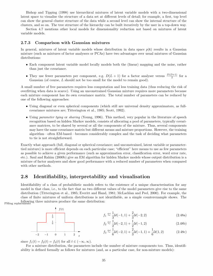
Bishop and Tipping (1998) use hierarchical mixtures of latent variable models with a two-dimensionallatent space to visualise the structure of a data set at different levels of detail; for example, a first, top levelcan show the general cluster structure of the data while a second level can show the internal structure of theclusters, and so on. The tree structure of the hierarchy can be built iteratively by the user in a top-down way.

Section 4.7 mentions other local models for dimensionality reduction not based on mixtures of latentvariable models.

2.7.3 Comparison with Gaussian mixtures

In general, mixtures of latent variable models whose distribution in data space p(t) results in a Gaussianmixture (such as mixtures of factor analysers or PCAs) have two advantages over usual mixtures of Gaussiandistributions:

• Each component latent variable model locally models both the (linear) mapping and the noise, ratherthan just the covariance.

• They use fewer parameters per component, e.g. D(L + 1) for a factor analyser versus D(D+1)2 for a

Gaussian (of course, L should not be too small for the model to remain good).

A small number of free parameters requires less computation and less training data (thus reducing the risk ofoverfitting when data is scarce). Using an unconstrained Gaussian mixture requires more parameters becauseeach mixture component has its own covariance matrix. The total number of parameters can be reduced byone of the following approaches:

• Using diagonal or even spherical components (which still are universal density approximators, as full-covariance mixtures are; Titterington et al., 1985; Scott, 1992).

• Using parameter tying or sharing (Young, 1996). This method, very popular in the literature of speechrecognition based on hidden Markov models, consists of allocating a pool of parameters, typically covari-ance matrices, to be shared by several or all the components of the mixture. Thus, several componentsmay have the same covariance matrix but different means and mixture proportions. However, the trainingalgorithm—often EM-based—becomes considerably complex and the task of deciding what parametersto tie is not straightforward.

Exactly what approach (full, diagonal or spherical covariance; and unconstrained, latent variable or parameter-tied mixture) is more efficient depends on each particular case; “efficient” here means to use as few parametersas possible to achieve a given performance (such as approximation error, classification error, word error rate,etc.). Saul and Rahim (2000b) give an EM algorithm for hidden Markov models whose output distribution is amixture of factor analysers and show good performance with a reduced number of parameters when comparedwith other methods.

2.8 Identifiability, interpretability and visualisation

Identifiability of a class of probabilistic models refers to the existence of a unique characterisation for anymodel in that class, i.e., to the fact that no two different values of the model parameters give rise to the samedistribution (Titterington et al., 1985; Everitt and Hand, 1981; McLachlan and Peel, 2000). For example, theclass of finite mixtures of uniform distributions is not identifiable, as a simple counterexample shows. Thefollowing three mixtures produce the same distribution:

PSfrag replacements

t

f(t)

16

13

−2 −1 0 1 2

f1def∼ 1

3U(−1, 1) +

2

3U(−2, 2) (2.48a)

f2def∼ 1

2U(−2, 1) +

1

2U(−1, 2) (2.48b)

f3def∼ 1

6U(−2, 1) +

2

3U(−1, 1) +

1

6U(1, 2) (2.48c)

since f1(t) = f2(t) = f3(t) for all t ∈ (−∞,∞).For a mixture distribution, the parameters include the number of mixture components too. Thus, identifi-

ability is defined formally as follows for mixtures (and, as a particular case, for non-mixture models):

35

Definition 2.8.1. A class of finite mixtures parameterised by Θ is said to be identifiable if for any twomembers

p(t;Θ)def=

M∑

m=1

πmp(t; θm) p(t;Θ∗)def=

M∗∑

m=1

π∗mp(t; θ

∗m)

then p(t;Θ) = p(t;Θ∗) for all t ∈ T if and only if M = M∗ and πm = π∗m and θm = θ∗m for m = 1, . . . ,M

(perhaps with a reordering of the indices). Trivial cases where πm = 0 or θm = θm′ for some m, m′ aredisregarded, being exactly represented by a mixture with fewer components.

Consider the example of equations (2.48). Given a sample {tn}Nn=1 generated from f1, we cannot tell fromwhich of f1, f2 or f3 it was generated (given the sample alone). Estimating the parameters of a uniformmixture with two components could end up (approximately) in any of f1 or f2 or not work at all, dependingon the algorithm used, the starting point if it is iterative, etc. The sample could be interpreted as coming fromtwo populations (in the case of f1 and f2) or from three (in the case of f3). Thus, if we want (1) to be ableto interpret in a unique way the parameters estimated from a sample, and (2) to avoid that the estimationprocedure may break down in case of ill-posedness, then the model class being considered must be identifiable.

However, theoretical identifiability is not the whole story:

• The existence of local, suboptimal maxima of the log-likelihood (or other objective function) makes verydifficult to obtain the global maximum—for example, when estimating a Gaussian mixture or a GTMmodel (fig. 2.13).

• Theoretical identifiability does not guarantee practical identifiability, as discussed in section 3.3.3.2.

Non-identifiability often arises with discrete distributions, for the following reason: if there are C categorieswe cannot set up more than C − 1 independent equations (because

∑p(c) = 1) and hence can only determine

C−1 parameters at most. Fortunately, with continuous distributions—the case that concerns us—it is usuallynot a problem.

Identifiability is a mathematical property that depends on the choice of model and there are no generalnecessary and sufficient conditions for all models. The identifiability of the latent variable models of section 2.6,if known, is discussed below, while that of finite mixtures of multivariate Bernoulli distributions (which areused in chapter 5) is discussed separately in section 3.3. A further treatment of the identifiability of mixturesis given by Titterington et al. (1985).

2.8.1 Interpretability

The factor analysis literature, especially regarding social science applications, has debated the issue of theinterpretability of factors for decades. The problem arises from the fact that factor analysis is non-identifiablewith respect to orthogonal rotations of the factors.

As noticed in section 2.3.2, in an ideal latent variable model we could adjust freely both the latent spaceprior distribution pl(x) and the mapping f via an invertible transformation g of the latent space, so that wecould have infinitely many equivalent combinations (pl, f), all giving rise to the same data distribution p(t) ineq. (2.3). In other words, we could have infinitely many different coordinate systems, each one with its oneinterpretation, equally able to explain the data. In more practical latent variable models only some restrictedkinds of indeterminacy will exist (such as orthogonal rotations in factor analysis) but the point remains: thereis no empirical ground to prefer one model over another if both give rise to the same p(t).

The key matter is that the only variables with a real existence are the observed variables and that thelatent variables are sheer mathematical constructs subordinated to explaining the observed ones in a compactway (Bartholomew, 1987; Everitt, 1984). Therefore, one should not try to reify the latent variables34 or looktoo hard for an interpretation of the estimated parameters if the model under consideration belongs to annon-identifiable class. Also, one should not attribute a causal nature to the latent variables: the generativeview of section 2.3 is just a convenient conceptualisation of the probabilistic latent variable framework.

In contrast, let us mention the technique of principal variables (McCabe, 1984), related to principalcomponent analysis, whose aim is to select a subset of variables that contain, in some sense, as much informationas possible. The principal variables can be readily interpreted because they are observed variables—unlike theprincipal components, which are linear combinations of the observed variables.

34Although in some particular cases this may be possible. For example, Kvalheim (1992) claims that, in chemistry, latentvariables are often interpretable and independently verifiable.

36

However, what can be interpretable is the manifold in data space spanned by the mapping from latentonto data space, M = f(X ). This manifold is invariant under a coordinate change, while the coordinatesthemselves (the latent variables) are not. As an example, consider PCA: what reason is there to choose aparticular basis of the hyperplane spanned by the principal components? Besides, sample-based estimates of theprincipal components can vary considerably, in particular when the covariance matrix has several eigenvaluesof approximately the same value, since the directions of the associated eigenvectors will be strongly influencedby the noise. But the subspace spanned by those principal components is still unique and thus identifiableand interpretable.

Another issue is that often the model assumptions are wrong for the problem under consideration, due tothe nature of the relationship between variables being unknown or to the mathematical impossibility of usingan appropriate but overly complex model. Consider, for example, fitting a principal component analysis tothe data of figure 2.13. Interpretation of the estimated parameters in such a situation may be completelymisleading. Yet another difficulty lies in whether the number of parameters in the model and the way it isestimated from a data set can lead to overfitting.

Fortunately, in machine learning applications the data is usually of a very high dimensionality and therelationships between variables is nonlinear, so that more often than not the user does not have strong precon-ceptions about what the latent variables should be. Besides, as a consequence of the philosophical approachof statistical machine learning, which pursues to simulate the behaviour of a system, the utility of a modelis related to how well it can extract the structure of a high-dimensional data set—irrespective of whether itactually matches the true underlying system (always an idealisation anyway) or just mimicks it. Of course,overfitting remains a difficult problem.

To summarise:

• In the ideal case where we know the model from which the data comes (i.e., we know the number oflatent variables and the functional forms for the prior distribution in latent space, the mapping and thenoise model) and all is necessary is to fit its parameters, we need to check the issues of identifiabilityand overfitting.

• If we are guessing the model, apart from the identifiability and overfitting we need to assess the model’sgoodness, which is very difficult in high-dimensional cases when there are nonlinear relationships. Forexample, the noise can easily mask nonlinear relationships when using a linear model.

2.8.2 Identifiability of specific latent variable models

2.8.2.1 Factor analysis

From section 2.6.1 we know that:

• If L > 1 then an orthogonal rotation of the factors produces the same data distribution, so that factoranalysis is non-identifiable with respect to orthogonal rotations. If L = 1 then the rotation becomes asign reversal, which is irrelevant.

• If we consider a generalised view of factor analysis where the factors are distributed normally but notnecessarily N (0, I), then factor analysis is non-identifiable with respect to any invertible linear transfor-mation of the factors.

In confirmatory factor analysis, where some elements of the loading matrix Λ are fixed, the rotation indeter-minacy may disappear. In explanatory factor analysis, where all elements of Λ are free, one usually applies arestriction to make it identifiable. The most typical one is to choose the factors so that the first factor makesa maximum contribution to the variance of the observed variables, the second makes a maximum contributionsubject to being uncorrelated with the first one, and so on. This can be shown to be equivalent to choosing Λsuch that ΛTΨ−1Λ is diagonal and has the effect of imposing 1

2L(L− 1) constraints, so that the total numberof free parameters becomes

D︸︷︷︸

Ψ

+ DL︸︷︷︸

Λ

+1

2L(L− 1)︸ ︷︷ ︸

constraints

which for consistency must be smaller or equal than the number of elements in the covariance matrix, 12D(D+

1), i.e., 12 ((D − L)2 − (D + L)) must be positive, which gives an upper bound for the number of factors to be

extracted.

37

Since scale changes of the data (t′ = Dt with D diagonal) result in an irrelevant scale change of the factorsand the uniquenesses, the same results are obtained whether using the covariance matrix or the correlationmatrix.

2.8.2.2 PCA

PCA as defined in section 2.6.2 only differs from factor analysis in the noise model and is constrained to producethe principal components in decreasing order of their associated variance, i.e., ΛT (σ2I)−1Λ is diagonal fromeq. (2.28). Thus, PCA is always identifiable except when several eigenvalues of the sample covariance matrixare equal, in which case the corresponding eigenvectors (columns of UL) can be rotated orthogonally insidetheir own subspace at will.

Unlike with factor analysis, with PCA different results are obtained whether using the covariance matrixor the correlation matrix because there is a single uniqueness parameter shared by all data variables. PCAdoes depend on the scale, so one has to decide whether to sphere the data or not.

2.8.2.3 ICA

Arbitrary scaling, reordering or in general invertible linear mapping of the latent variables (sources) givesrise to the same observed (sensor) distribution: (Λ,x), (ΛV,V−1x), (ΛP,PTx) and (ΛR,R−1x) all producethe same distribution p(t) if V is diagonal nonsingular, P is a permutation matrix and R is nonsingular.However, only scaling and reordering are acceptable indeterminacies, because they do not alter the “waveformof the signals” or their statistical properties (independence in particular). Thus, it can be proven that theidentifiability of the ICA model (up to reordering and rescaling) is guaranteed if (Tong et al., 1991; Comon,1994):

• At most one source is distributed normally (since the sum of two normals is itself normal, it would notpossible to separate the individual components in a unique way).

• There are fewer sources than sensors: L ≤ D.

• The mixing matrix is full-rank: rank (Λ) = L.

2.8.2.4 Other latent variable models

To our knowledge, no identifiability results are known for GTM, IFA or mixtures of factor analysers or principalcomponent analysers—but suboptimal local maxima of the log-likelihood do exist for all of them.

2.8.3 Visualisation

A different matter from interpretability is visualisation of data. While all coordinate systems related by aninvertible map (reparametrisation) are equivalent for dimensionality reduction, some may be more appropriatethan others in that the structure in the data is shown more clearly. Rigid motion transformations (translation,rotation or reflection) have a trivial effect on visualisation, since our visual system can still recognise thestructure in the data, but invertible transformations that alter the distances between points (distortions) canboth make apparent but also completely mask clusters or other accidents in the data.

It is possible to include constraints in the latent variable model being used to ensure that the interpointdistances in data space are approximately preserved in the latent space. These constraints affect exclusivelythe mapping f . However, if the prior distribution in latent space is not flexible enough to represent a largeclass of distributions (and it is not for factor analysis, PCA and GTM, since it is fixed) then by constrainingf we are reducing the class of distributions that the model can approximate.

These distortion constraints are different from the usual smoothness constraints: the latter force the man-ifold M = f(X ) traced by the function f to be smooth but do not care about the coordinate system (theparametrisation); they usually bound (in a soft fashion) the second derivative of f . In contrast, the distortionconstraints do not care whether the manifold M is smooth or rough, but force the distances in data space tobe preserved in latent space. How this is done depends on how the distance between two data space points isdefined: as geodetic distance (i.e., following the shortest path between the two points along the data manifold,

38

in which case it is appropriate to use a unit-speed parametrisation35 that bounds the first derivative of f) oras Euclidean distance (i.e., following the straight line segment joining both points freely in the data space,whether it goes out of the data manifold or not). This consideration enters the realm of distance-preservingmethods and multidimensional scaling, briefly described in section 4.10.

Such distortion constraints can be incorporated as a regularisation term in the log-likelihood or, equiv-alently, viewed as a prior distribution on the parameters of f . In any case they lead to the appearance ofhyperparameters that control the relative importance of the fitting term (log-likelihood) and the regularisa-tion term (distortion constraint). Determining good values for the hyperparameters is a well-known problemthat we will meet several times in this thesis, but on which we shall not dwell.

For example, it has been observed that the estimates found by GTM often give a distorted view of thedata due to the latent space stretching like a rubber sheet (Tenenbaum, 1998; Marrs and Webb, 1999). Thismetric distortion is revealed by high values of an appropriately defined magnification factor. A magnificationfactor M(x) is a scalar function dependent on the latent space point that measures the local distortion atlatent space point x induced by the mapping f : X → T . Bishop et al. (1997b) defined it in the usual sense ofdifferential geometry as the ratio of hypervolumes in the data space and the latent space, equal to the Jacobian

of the mapping f : M(x;W)def= dVT

dVX= Jf =

√

|KTWTWK| where (K)fldef=

∂φf

∂xl. A value of one for this

magnification factor corresponds to no distortion (although Marrs and Webb (1999) have pointed out thatit can also be one for some distortions; their slightly different definition of the magnification factor is givenbelow). Marrs and Webb (1999) implement an average generalised unit-speed constraint in GTM’s function fto preserve geodetic distances:

Ep(t){KTWTWK

}= IL

which for a one-dimensional latent space (L = 1) reduces to E{∥∥ dfdx

∥∥

2}

= 1, i.e., a parametrisation of average

unit squared speed. This constraint results in a modified M step of the EM algorithm for GTM, eq. (2.45a).

The results can be evaluated by checking that the magnification factor M(x;W)def=∥∥KTWTWK− I

∥∥

2(a

zero value of which corresponds to no distortion) is small in all points of the latent space.

2.9 Mapping from data onto latent space

2.9.1 Dimensionality reduction and vector reconstruction

In dimensionality reduction (reviewed in chapter 4) we want, given a data point t, to obtain a representativeof it in latent space, x∗ = F(t), for a certain mapping F : T −→ X . The latent variable modelling frameworkallows the definition of a natural dimensionality reduction mapping. Once the parameters36 Θ are fixed,Bayes’ theorem gives the posterior distribution in latent space given a data vector t, i.e., the distribution ofthe probability that a point x in latent space was responsible for generating t:

p(x|t) =p(t|x)p(x)

p(t)=

p(t|x)p(x)∫

X p(t|x)p(x) dx. (2.49)

The latent variable model gives us all this information about x for fixed t. Summarising this distributionx|t in a single latent space point x∗ results in a reduced-dimension representative37 of t. This definesa corresponding mapping F from data space onto latent space, so that every data point t is assigned arepresentative in latent space, x∗ = F(t). Thus, it can be considered as an inverse mapping of f .

35For a curve f : x ∈ R → RD, a unit-speed parametrisation verifies∥∥∥

dfdx

∥∥∥

2=∑D

d=1

(dfddx

)2= 1. Equivalently, the arc length

between two points f(x1) and f(x2) on the curve is∣∣∣∣∣

∫ x2

x1

√∑D

d=1

(dfddx

)2dx

∣∣∣∣∣= |x2 − x1|

so that this parametrisation is also called arc-length parametrisation. It means that a unit step in latent space produces a unitstep along the curve in data space.

36In what follows, we omit the parameters from the formulae for clarity, i.e., p(x|t) really means p(x|t,Θ), and so on.37Admittedly, reduced-dimension representative of an observed point t is a pedantic denomination, but it points to the two

things we are interested in: that it (1) represents the observed point (2) in latent space. Latent space representative is alsoacceptable, although less general. Other, more compact terms have been proposed but we find them unsatisfactory. For example,cause of an observed point t may attribute to the reduced-dimension representative more than it really is worth (and ring unwantedbells concerning its interpretation). And the term scores, very popular in statistics, sounds too vague.

39

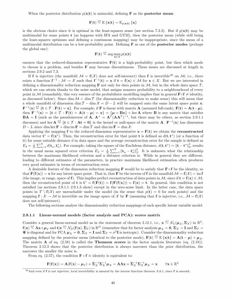
When the posterior distribution p(x|t) is unimodal, defining F as the posterior mean:

F(t)def= E {x|t} = Ep(x|t) {x}

is the obvious choice since it is optimal in the least-squares sense (see section 7.3.3). But if p(x|t) may bemultimodal for some points t (as happens with IFA and GTM), then the posterior mean (while still beingthe least-squares optimum and defining a continuous mapping) may be inappropriate, since the mean of amultimodal distribution can be a low-probability point. Defining F as one of the posterior modes (perhapsthe global one):

F(t)def= arg max

x∈Xp(x|t)

ensures that the reduced-dimension representative F(t) is a high-probability point, but then which modeto choose is a problem, and besides F may become discontinuous. These issues are discussed at length insections 2.9.2 and 7.3.

If f is injective (the manifold M = f(X ) does not self-intersect) then f is invertible38 on M; i.e., thereexists a function f−1 : M → X such that f−1(t) = x if t = f(x) ∈ M for x ∈ X . But we are interested indefining a dimensionality reduction mapping F not only for data points inM, but in the whole data space T ,which we can attain thanks to the noise model, that assigns nonzero probability to a neighbourhood of everypoint inM (remarkably, this very essence of the probabilistic modelling implies that in general F◦f 6= identity,as discussed below). Since dimM < dim T (for dimensionality reduction to make sense) this will mean thata whole manifold of dimension dim T − dimX = D − L will be mapped onto the same latent space point x:

F−1(x)def= {t ∈ T : F(t) = x}. For example, if F is linear with matrix A (assumed full-rank), F(t) = A(t−µ),

then F−1(x) = {t ∈ T : F(t) = A(t − µ) = x} = {µ + Bx} + kerA where B is any matrix that satisfiesBA = I (such as the pseudoinverse of A, A+ = AT (AAT )−1, but there may be others, as section 2.9.1.1

discusses) and kerAdef= {t ∈ T : At = 0} is the kernel or null-space of the matrix A. F−1(x) has dimension

D − L since dim kerF + dim imF = dim T and dim imF = dimX .Applying the mapping f to the reduced-dimension representative x = F(t) we obtain the reconstructed

data vector t∗ = f(x∗). Then, the reconstruction error for that point t is defined as d(t, t∗) (or a function ofit) for some suitable distance d in data space and the average reconstruction error for the sample is defined as

Ed = 1N

∑Nn=1 d(tn, t

∗n). For example, taking the square of the Euclidean distance, d(t, t∗) = ‖t− t∗‖22, results

in the usual mean squared error criterion E2 = 1N

∑Nn=1 ‖tn − t∗n‖22. It is unknown what the relationship

between the maximum likelihood criterion and a distance criterion is. While in general they are different,leading to different estimates of the parameters, in practice maximum likelihood estimation often producesvery good estimates in terms of reconstruction error.

A desirable feature of the dimension reduction mapping F would be to satisfy that F ◦ f be the identity, sothat F(f(x)) = x for any latent space point. That is, that F be the inverse of f in the manifoldM = f(X ) = im f(the image, or range, space of f). This implies perfect reconstruction of data points inM, since if t = f(x) ∈M,then the reconstructed point of t is t∗ = f(F(t)) = f(F(f(x))) = f(x) = t. In general, this condition is notsatisfied (as sections 2.9.1.1–2.9.1.3 show) except in the zero-noise limit. In the latter case, the data spacepoints in T \ f(X ) are unreachable under the model (in the sense that p(t) = 0 for such points) and themapping f : X →M is invertible on the image space of X by F (assuming that f is injective, i.e., M = f(X )does not self-intersect).

The following sections analyse the dimensionality reduction mappings of each specific latent variable model.

2.9.1.1 Linear-normal models (factor analysis and PCA): scores matrix

Consider a general linear-normal model as in the statement of theorem 2.12.1, i.e., xdef∼ NL(µX ,ΣX) in RL,

f(x)def= Λx+µT and t|x def∼ ND(f(x),ΣT ) in RD (remember that for factor analysis µX = 0, ΣX = I and ΣT =

Ψ is diagonal and for PCA µX = 0, ΣX = I and ΣT = σ2I is isotropic). Consider the dimensionality reduction

mapping defined by the posterior mean (identical to the posterior mode), F(t)def= E {x|t} = A(t− µ) + µX .

The matrix A of eq. (2.58) is called the Thomson scores in the factor analysis literature (eq. (2.18)).Theorem 2.12.3 shows that the posterior distribution is always narrower than the prior distribution, thenarrower the smaller the noise is.

From eq. (2.57), the condition F ◦ f ≡ identity is equivalent to:

F(f(x)) = A(f(x)− µT ) + Σ−1X Σ−1

X µX = AΛx + Σ−1X Σ−1

X µX = x ∀x ∈ RL

38And even if f is not injective, local invertibility is assured by the inverse function theorem A.6.1, since f is smooth.

40

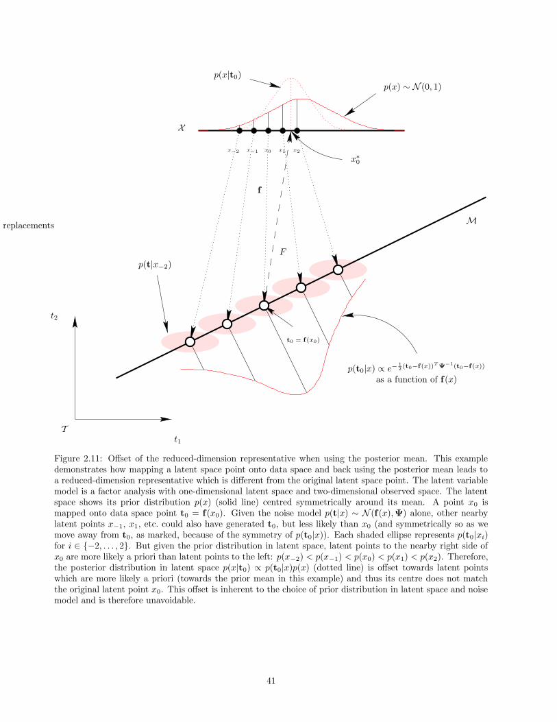
PSfrag replacements

X

M

x−2 x−1 x0 x1 x2

t0 = f(x0)

t1

t2

T

f

F

p(x) ∼ N (0, 1)

p(t0|x) ∝ e−12 (t0−f(x))T Ψ−1(t0−f(x))

as a function of f(x)

p(t|x−2)

p(x|t0)

x∗0

Figure 2.11: Offset of the reduced-dimension representative when using the posterior mean. This exampledemonstrates how mapping a latent space point onto data space and back using the posterior mean leads toa reduced-dimension representative which is different from the original latent space point. The latent variablemodel is a factor analysis with one-dimensional latent space and two-dimensional observed space. The latentspace shows its prior distribution p(x) (solid line) centred symmetrically around its mean. A point x0 ismapped onto data space point t0 = f(x0). Given the noise model p(t|x) ∼ N (f(x),Ψ) alone, other nearbylatent points x−1, x1, etc. could also have generated t0, but less likely than x0 (and symmetrically so as wemove away from t0, as marked, because of the symmetry of p(t0|x)). Each shaded ellipse represents p(t0|xi)for i ∈ {−2, . . . , 2}. But given the prior distribution in latent space, latent points to the nearby right side ofx0 are more likely a priori than latent points to the left: p(x−2) < p(x−1) < p(x0) < p(x1) < p(x2). Therefore,the posterior distribution in latent space p(x|t0) ∝ p(t0|x)p(x) (dotted line) is offset towards latent pointswhich are more likely a priori (towards the prior mean in this example) and thus its centre does not matchthe original latent point x0. This offset is inherent to the choice of prior distribution in latent space and noisemodel and is therefore unavoidable.

41

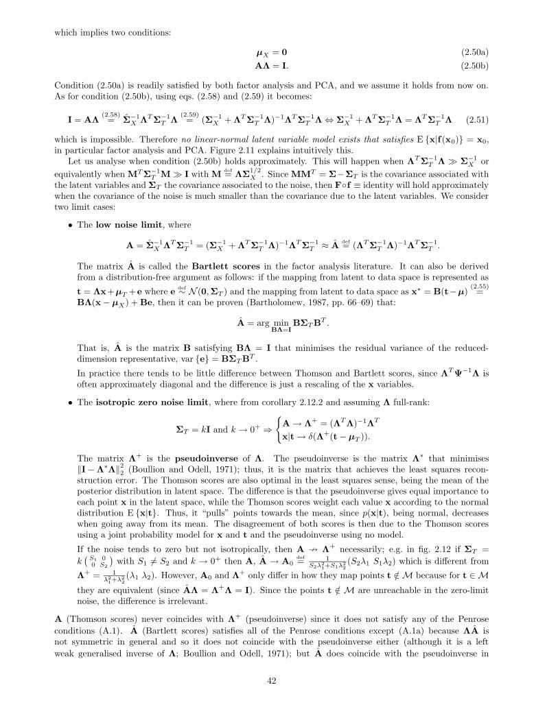
which implies two conditions:

µX = 0 (2.50a)

AΛ = I. (2.50b)

Condition (2.50a) is readily satisfied by both factor analysis and PCA, and we assume it holds from now on.As for condition (2.50b), using eqs. (2.58) and (2.59) it becomes:

I = AΛ(2.58)= Σ−1

X ΛTΣ−1T Λ

(2.59)= (Σ−1

X + ΛTΣ−1T Λ)−1ΛTΣ−1

T Λ⇔ Σ−1X + ΛTΣ−1

T Λ = ΛTΣ−1T Λ (2.51)

which is impossible. Therefore no linear-normal latent variable model exists that satisfies E {x|f(x0)} = x0,in particular factor analysis and PCA. Figure 2.11 explains intuitively this.

Let us analyse when condition (2.50b) holds approximately. This will happen when ΛTΣ−1T Λ � Σ−1

X or

equivalently when MTΣ−1T M� I with M

def= ΛΣ

1/2X . Since MMT = Σ−ΣT is the covariance associated with

the latent variables and ΣT the covariance associated to the noise, then F◦f ≡ identity will hold approximatelywhen the covariance of the noise is much smaller than the covariance due to the latent variables. We considertwo limit cases:

• The low noise limit, where

A = Σ−1X ΛTΣ−1

T = (Σ−1X + ΛTΣ−1

T Λ)−1ΛTΣ−1T ≈ A

def= (ΛTΣ−1

T Λ)−1ΛTΣ−1T .

The matrix A is called the Bartlett scores in the factor analysis literature. It can also be derivedfrom a distribution-free argument as follows: if the mapping from latent to data space is represented as

t = Λx+µT +e where edef∼ N (0,ΣT ) and the mapping from latent to data space as x∗ = B(t−µ)

(2.55)=

BΛ(x− µX) + Be, then it can be proven (Bartholomew, 1987, pp. 66–69) that:

A = arg minBΛ=I

BΣTBT .

That is, A is the matrix B satisfying BΛ = I that minimises the residual variance of the reduced-dimension representative, var {e} = BΣTBT .

In practice there tends to be little difference between Thomson and Bartlett scores, since ΛTΨ−1Λ isoften approximately diagonal and the difference is just a rescaling of the x variables.

• The isotropic zero noise limit, where from corollary 2.12.2 and assuming Λ full-rank:

ΣT = kI and k → 0+ ⇒{

A→ Λ+ = (ΛTΛ)−1ΛT

x|t→ δ(Λ+(t− µT )).

The matrix Λ+ is the pseudoinverse of Λ. The pseudoinverse is the matrix Λ∗ that minimises‖I−Λ∗Λ‖22 (Boullion and Odell, 1971); thus, it is the matrix that achieves the least squares recon-struction error. The Thomson scores are also optimal in the least squares sense, being the mean of theposterior distribution in latent space. The difference is that the pseudoinverse gives equal importance toeach point x in the latent space, while the Thomson scores weight each value x according to the normaldistribution E {x|t}. Thus, it “pulls” points towards the mean, since p(x|t), being normal, decreaseswhen going away from its mean. The disagreement of both scores is then due to the Thomson scoresusing a joint probability model for x and t and the pseudoinverse using no model.

If the noise tends to zero but not isotropically, then A 9 Λ+ necessarily; e.g. in fig. 2.12 if ΣT =

k(S1 00 S2

)with S1 6= S2 and k → 0+ then A, A → A0

def= 1

S2λ21+S1λ2

2(S2λ1 S1λ2) which is different from

Λ+ = 1λ2

1+λ22(λ1 λ2). However, A0 and Λ+ only differ in how they map points t /∈M because for t ∈M

they are equivalent (since AΛ = Λ+Λ = I). Since the points t /∈ M are unreachable in the zero-limitnoise, the difference is irrelevant.

A (Thomson scores) never coincides with Λ+ (pseudoinverse) since it does not satisfy any of the Penrose

conditions (A.1). A (Bartlett scores) satisfies all of the Penrose conditions except (A.1a) because ΛA isnot symmetric in general and so it does not coincide with the pseudoinverse either (although it is a left

weak generalised inverse of Λ; Boullion and Odell, 1971); but A does coincide with the pseudoinverse in

42

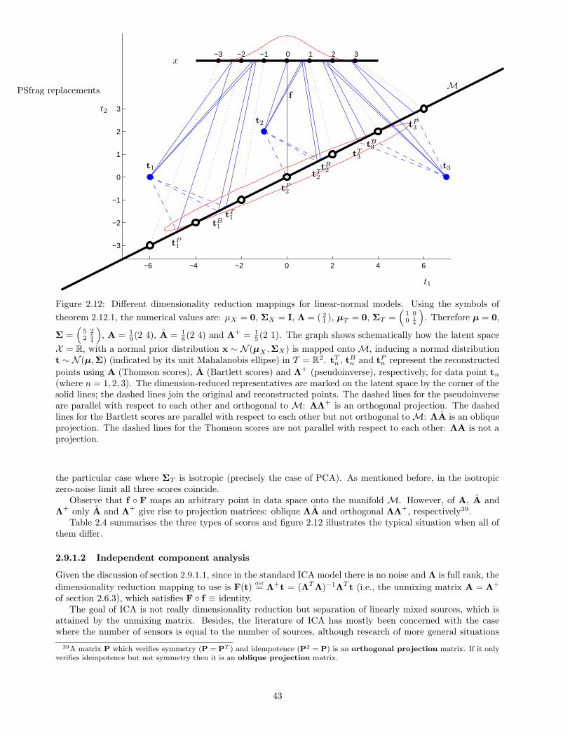
−6 −4 −2 0 2 4 6

−3

−2

−1

0

1

2

3

−3 −2 −1 0 1 2 3

PSfrag replacements

x

M

t1

t2

f

t1

tT1tB1

tP1

t2

tT2tB2

tP2

t3

tT3

tB3

tP3

Figure 2.12: Different dimensionality reduction mappings for linear-normal models. Using the symbols of

theorem 2.12.1, the numerical values are: µX = 0, ΣX = I, Λ = ( 21 ), µT = 0, ΣT =

(1 00 1

4

)

. Therefore µ = 0,

Σ =(

5 22 5

4

)

, A = 19 (2 4), A = 1

8 (2 4) and Λ+ = 15 (2 1). The graph shows schematically how the latent space

X = R, with a normal prior distribution x ∼ N (µX ,ΣX) is mapped onto M, inducing a normal distributiont ∼ N (µ,Σ) (indicated by its unit Mahalanobis ellipse) in T = R2. tTn , tBn and tPn represent the reconstructed

points using A (Thomson scores), A (Bartlett scores) and Λ+ (pseudoinverse), respectively, for data point tn(where n = 1, 2, 3). The dimension-reduced representatives are marked on the latent space by the corner of thesolid lines; the dashed lines join the original and reconstructed points. The dashed lines for the pseudoinverseare parallel with respect to each other and orthogonal to M: ΛΛ+ is an orthogonal projection. The dashedlines for the Bartlett scores are parallel with respect to each other but not orthogonal toM: ΛA is an obliqueprojection. The dashed lines for the Thomson scores are not parallel with respect to each other: ΛA is not aprojection.

the particular case where ΣT is isotropic (precisely the case of PCA). As mentioned before, in the isotropiczero-noise limit all three scores coincide.

Observe that f ◦ F maps an arbitrary point in data space onto the manifold M. However, of A, A andΛ+ only A and Λ+ give rise to projection matrices: oblique ΛA and orthogonal ΛΛ+, respectively39.

Table 2.4 summarises the three types of scores and figure 2.12 illustrates the typical situation when all ofthem differ.

2.9.1.2 Independent component analysis

Given the discussion of section 2.9.1.1, since in the standard ICA model there is no noise and Λ is full rank, the

dimensionality reduction mapping to use is F(t)def= Λ+t = (ΛTΛ)−1ΛT t (i.e., the unmixing matrix A = Λ+

of section 2.6.3), which satisfies F ◦ f ≡ identity.The goal of ICA is not really dimensionality reduction but separation of linearly mixed sources, which is

attained by the unmixing matrix. Besides, the literature of ICA has mostly been concerned with the casewhere the number of sensors is equal to the number of sources, although research of more general situations

39A matrix P which verifies symmetry (P = PT ) and idempotence (P2 = P) is an orthogonal projection matrix. If it onlyverifies idempotence but not symmetry then it is an oblique projection matrix.

43

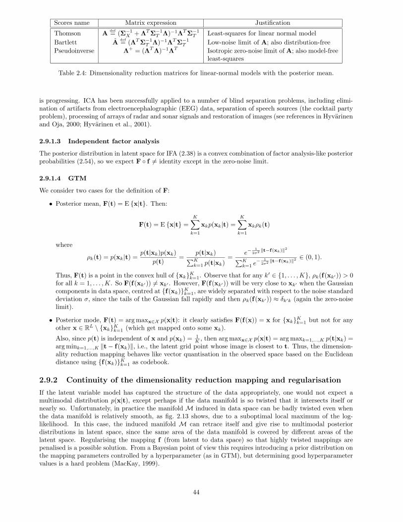
Scores name Matrix expression Justification

Thomson Adef= (Σ−1

X + ΛTΣ−1T Λ)−1ΛTΣ−1

T Least-squares for linear normal model

Bartlett Adef= (ΛTΣ−1

T Λ)−1ΛTΣ−1T Low-noise limit of A; also distribution-free

Pseudoinverse Λ+ = (ΛTΛ)−1ΛT Isotropic zero-noise limit of A; also model-freeleast-squares

Table 2.4: Dimensionality reduction matrices for linear-normal models with the posterior mean.

is progressing. ICA has been successfully applied to a number of blind separation problems, including elimi-nation of artifacts from electroencephalographic (EEG) data, separation of speech sources (the cocktail partyproblem), processing of arrays of radar and sonar signals and restoration of images (see references in Hyvarinenand Oja, 2000; Hyvarinen et al., 2001).

2.9.1.3 Independent factor analysis

The posterior distribution in latent space for IFA (2.38) is a convex combination of factor analysis-like posteriorprobabilities (2.54), so we expect F ◦ f 6= identity except in the zero-noise limit.

2.9.1.4 GTM

We consider two cases for the definition of F:

• Posterior mean, F(t) = E {x|t}. Then:

F(t) = E {x|t} =K∑

k=1

xkp(xk|t) =K∑

k=1

xkρk(t)

where

ρk(t) = p(xk|t) =p(t|xk)p(xk)

p(t)=

p(t|xk)∑Kk=1 p(t|xk)

=e−

12σ2 ‖t−f(xk)‖2

∑Kk=1 e

− 12σ2 ‖t−f(xk)‖2 ∈ (0, 1).

Thus, F(t) is a point in the convex hull of {xk}Kk=1. Observe that for any k′ ∈ {1, . . . ,K}, ρk(f(xk′)) > 0for all k = 1, . . . ,K. So F(f(xk′)) 6= xk′ . However, F(f(xk′)) will be very close to xk′ when the Gaussiancomponents in data space, centred at {f(xk)}Kk=1, are widely separated with respect to the noise standarddeviation σ, since the tails of the Gaussian fall rapidly and then ρk(f(xk′)) ≈ δk′k (again the zero-noiselimit).

• Posterior mode, F(t) = arg maxx∈X p(x|t): it clearly satisfies F(f(x)) = x for {xk}Kk=1 but not for anyother x ∈ RL \ {xk}Kk=1 (which get mapped onto some xk).

Also, since p(t) is independent of x and p(xk) = 1K , then arg maxx∈X p(x|t) = arg maxk=1,...,K p(t|xk) =

arg mink=1,...,K ‖t− f(xk)‖, i.e., the latent grid point whose image is closest to t. Thus, the dimension-ality reduction mapping behaves like vector quantisation in the observed space based on the Euclideandistance using {f(xk)}Kk=1 as codebook.

2.9.2 Continuity of the dimensionality reduction mapping and regularisation

If the latent variable model has captured the structure of the data appropriately, one would not expect amultimodal distribution p(x|t), except perhaps if the data manifold is so twisted that it intersects itself ornearly so. Unfortunately, in practice the manifold M induced in data space can be badly twisted even whenthe data manifold is relatively smooth, as fig. 2.13 shows, due to a suboptimal local maximum of the log-likelihood. In this case, the induced manifold M can retrace itself and give rise to multimodal posteriordistributions in latent space, since the same area of the data manifold is covered by different areas of thelatent space. Regularising the mapping f (from latent to data space) so that highly twisted mappings arepenalised is a possible solution. From a Bayesian point of view this requires introducing a prior distribution onthe mapping parameters controlled by a hyperparameter (as in GTM), but determining good hyperparametervalues is a hard problem (MacKay, 1999).

44

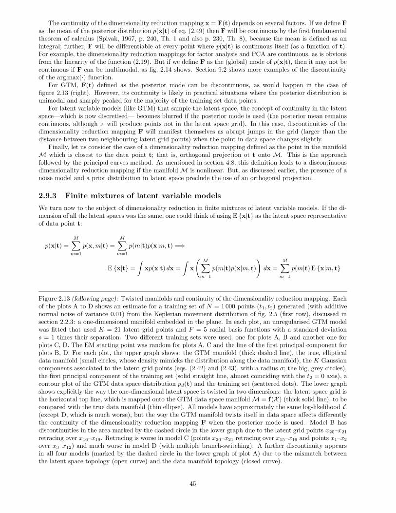
The continuity of the dimensionality reduction mapping x = F(t) depends on several factors. If we define Fas the mean of the posterior distribution p(x|t) of eq. (2.49) then F will be continuous by the first fundamentaltheorem of calculus (Spivak, 1967, p. 240, Th. 1 and also p. 230, Th. 8), because the mean is defined as anintegral; further, F will be differentiable at every point where p(x|t) is continuous itself (as a function of t).For example, the dimensionality reduction mappings for factor analysis and PCA are continuous, as is obviousfrom the linearity of the function (2.19). But if we define F as the (global) mode of p(x|t), then it may not becontinuous if F can be multimodal, as fig. 2.14 shows. Section 9.2 shows more examples of the discontinuityof the arg max(·) function.

For GTM, F(t) defined as the posterior mode can be discontinuous, as would happen in the case offigure 2.13 (right). However, its continuity is likely in practical situations where the posterior distribution isunimodal and sharply peaked for the majority of the training set data points.

For latent variable models (like GTM) that sample the latent space, the concept of continuity in the latentspace—which is now discretised— becomes blurred if the posterior mode is used (the posterior mean remainscontinuous, although it will produce points not in the latent space grid). In this case, discontinuities of thedimensionality reduction mapping F will manifest themselves as abrupt jumps in the grid (larger than thedistance between two neighbouring latent grid points) when the point in data space changes slightly.

Finally, let us consider the case of a dimensionality reduction mapping defined as the point in the manifoldM which is closest to the data point t; that is, orthogonal projection ot t onto M. This is the approachfollowed by the principal curves method. As mentioned in section 4.8, this definition leads to a discontinuousdimensionality reduction mapping if the manifoldM is nonlinear. But, as discussed earlier, the presence of anoise model and a prior distribution in latent space preclude the use of an orthogonal projection.

2.9.3 Finite mixtures of latent variable models

We turn now to the subject of dimensionality reduction in finite mixtures of latent variable models. If the di-mension of all the latent spaces was the same, one could think of using E {x|t} as the latent space representativeof data point t:

p(x|t) =

M∑

m=1

p(x,m|t) =

M∑

m=1

p(m|t)p(x|m, t) =⇒

E {x|t} =

∫

xp(x|t) dx =

∫

x

(M∑

m=1

p(m|t)p(x|m, t))

dx =

M∑

m=1

p(m|t) E {x|m, t}

Figure 2.13 (following page): Twisted manifolds and continuity of the dimensionality reduction mapping. Eachof the plots A to D shows an estimate for a training set of N = 1000 points (t1, t2) generated (with additivenormal noise of variance 0.01) from the Keplerian movement distribution of fig. 2.5 (first row), discussed insection 2.2.3: a one-dimensional manifold embedded in the plane. In each plot, an unregularised GTM modelwas fitted that used K = 21 latent grid points and F = 5 radial basis functions with a standard deviations = 1 times their separation. Two different training sets were used, one for plots A, B and another one forplots C, D. The EM starting point was random for plots A, C and the line of the first principal component forplots B, D. For each plot, the upper graph shows: the GTM manifold (thick dashed line), the true, ellipticaldata manifold (small circles, whose density mimicks the distribution along the data manifold), the K Gaussiancomponents associated to the latent grid points (eqs. (2.42) and (2.43), with a radius σ; the big, grey circles),the first principal component of the training set (solid straight line, almost coinciding with the t2 = 0 axis), acontour plot of the GTM data space distribution pd(t) and the training set (scattered dots). The lower graphshows explicitly the way the one-dimensional latent space is twisted in two dimensions: the latent space grid isthe horizontal top line, which is mapped onto the GTM data space manifoldM = f(X ) (thick solid line), to becompared with the true data manifold (thin ellipse). All models have approximately the same log-likelihood L(except D, which is much worse), but the way the GTM manifold twists itself in data space affects differentlythe continuity of the dimensionality reduction mapping F when the posterior mode is used. Model B hasdiscontinuities in the area marked by the dashed circle in the lower graph due to the latent grid points x20–x21

retracing over x16–x19. Retracing is worse in model C (points x20–x21 retracing over x15–x19 and points x1–x2

over x3–x12) and much worse in model D (with multiple branch-switching). A further discontinuity appearsin all four models (marked by the dashed circle in the lower graph of plot A) due to the mismatch betweenthe latent space topology (open curve) and the data manifold topology (closed curve).

45

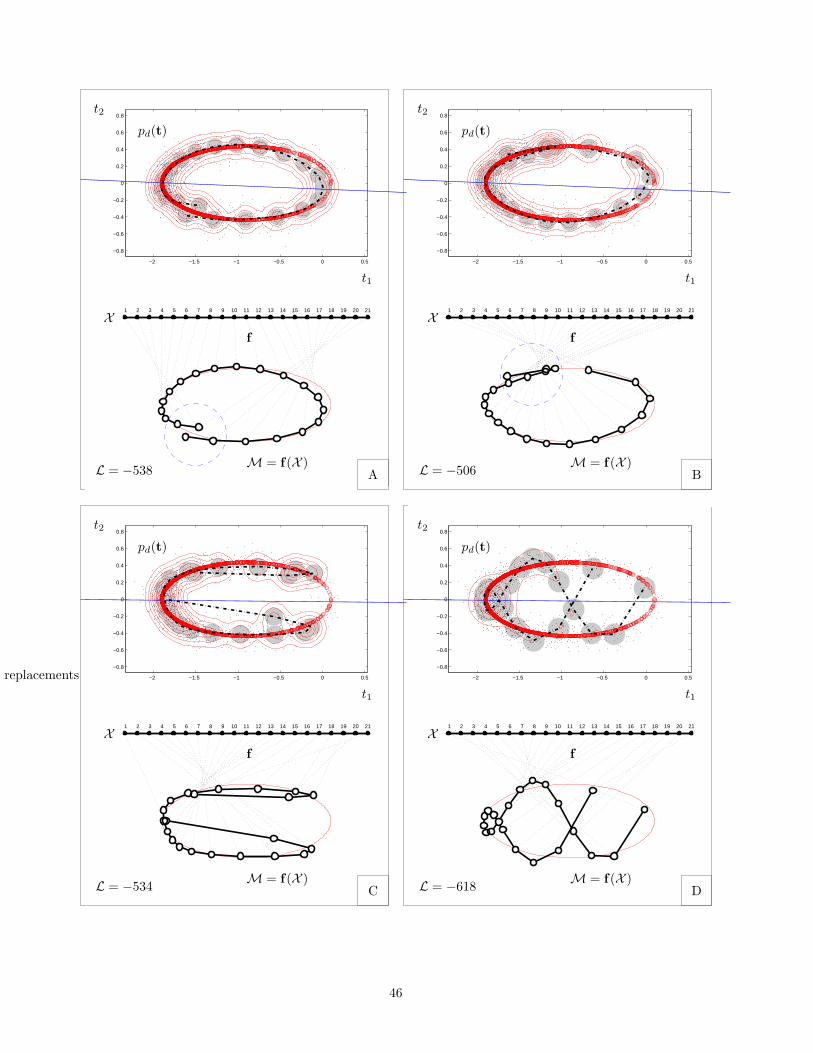
−2 −1.5 −1 −0.5 0 0.5

−0.8

−0.6

−0.4

−0.2

0

0.2

0.4

0.6

0.8

1 2 3 4 5 6 7 8 9 10 11 12 13 14 15 16 17 18 19 20 21

1 2 3 4 5 6 7 8 9 10 11 12 13 14 15 16 17 18 19 20 21

−2 −1.5 −1 −0.5 0 0.5

−0.8

−0.6

−0.4

−0.2

0

0.2

0.4

0.6

0.8

1 2 3 4 5 6 7 8 9 10 11 12 13 14 15 16 17 18 19 20 21

−2 −1.5 −1 −0.5 0 0.5

−0.8

−0.6

−0.4

−0.2

0

0.2

0.4

0.6

0.8

−2 −1.5 −1 −0.5 0 0.5

−0.8

−0.6

−0.4

−0.2

0

0.2

0.4

0.6

0.8

1 2 3 4 5 6 7 8 9 10 11 12 13 14 15 16 17 18 19 20 21

PSfrag replacements

A B

C D

t1

t1t1

t1

t2

t2t2

t2

pd(t)

pd(t)pd(t)

pd(t)

M = f(X )

M = f(X )M = f(X )

M = f(X )

f

ff

f

X

XX

X

L = −538 L = −506

L = −534 L = −618

46

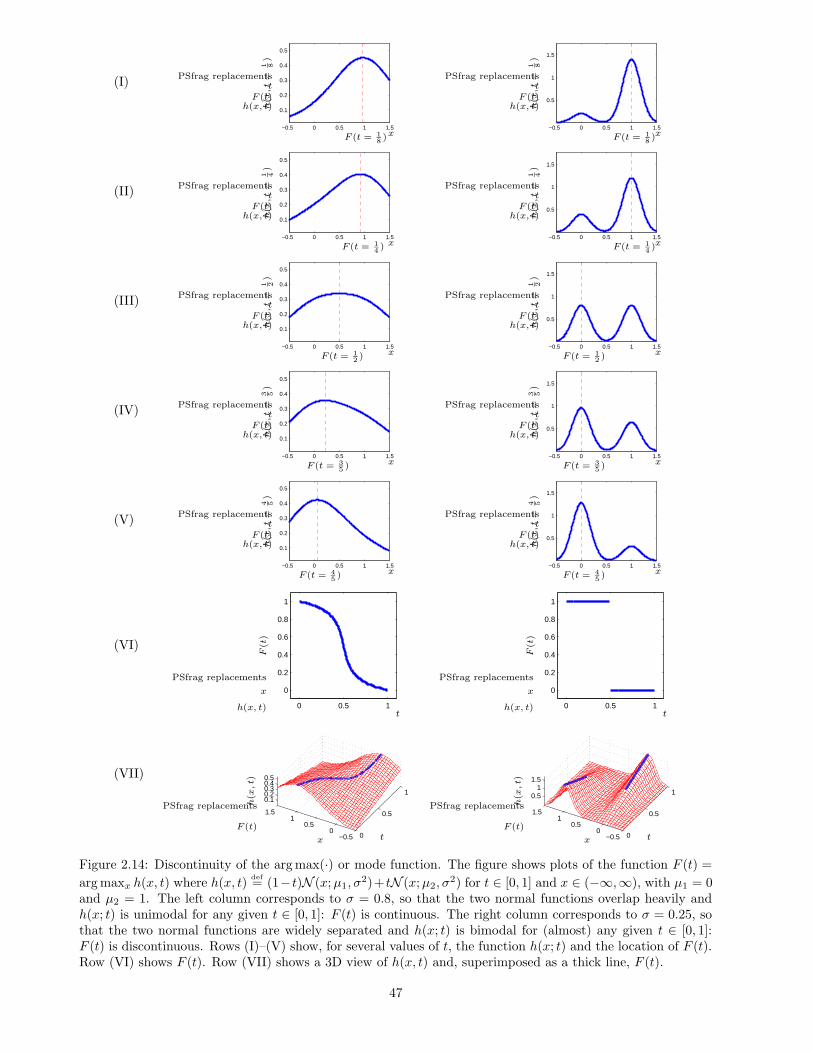
(I)

−0.5 0 0.5 1 1.5

0.1

0.2

0.3

0.4

0.5

PSfrag replacementst

x

F (t)h(x, t)

F (t = 18 )

h(x,t=

1 8)

−0.5 0 0.5 1 1.5

0.5

1

1.5

PSfrag replacementst

x

F (t)h(x, t)

F (t = 18 )

h(x,t=

1 8)

(II)

−0.5 0 0.5 1 1.5

0.1

0.2

0.3

0.4

0.5

PSfrag replacementst

x

F (t)h(x, t)

F (t = 14 )

h(x,t=

1 4)

−0.5 0 0.5 1 1.5

0.5

1

1.5

PSfrag replacementst

x

F (t)h(x, t)

F (t = 14 )

h(x,t=

1 4)

(III)

−0.5 0 0.5 1 1.5

0.1

0.2

0.3

0.4

0.5

PSfrag replacementst

x

F (t)h(x, t)

F (t = 12 )

h(x,t=

1 2)

−0.5 0 0.5 1 1.5

0.5

1

1.5

PSfrag replacementst

x

F (t)h(x, t)

F (t = 12 )

h(x,t=

1 2)

(IV)

−0.5 0 0.5 1 1.5

0.1

0.2

0.3

0.4

0.5

PSfrag replacementst

x

F (t)h(x, t)

F (t = 35 )

h(x,t=

3 5)

−0.5 0 0.5 1 1.5

0.5

1

1.5

PSfrag replacementst

x

F (t)h(x, t)

F (t = 35 )

h(x,t=

3 5)

(V)

−0.5 0 0.5 1 1.5

0.1

0.2

0.3

0.4

0.5

PSfrag replacementst

x

F (t)h(x, t)

F (t = 45 )

h(x,t=

4 5)

−0.5 0 0.5 1 1.5

0.5

1

1.5

PSfrag replacementst

x

F (t)h(x, t)

F (t = 45 )

h(x,t=

4 5)

(VI)

0 0.5 1

0

0.2

0.4

0.6

0.8

1

PSfrag replacements

t

x

F(t

)

h(x, t) 0 0.5 1

0

0.2

0.4

0.6

0.8

1

PSfrag replacements

t

x

F(t

)

h(x, t)

(VII)

0

0.5

1

−0.50

0.51

1.5

0.10.20.30.40.5

PSfrag replacements

tx

F (t)

h(x,t)

0

0.5

1

−0.50

0.51

1.5

0.51

1.5

PSfrag replacements

tx

F (t)

h(x,t)

Figure 2.14: Discontinuity of the arg max(·) or mode function. The figure shows plots of the function F (t) =

arg maxx h(x, t) where h(x, t)def= (1− t)N (x;µ1, σ

2)+ tN (x;µ2, σ2) for t ∈ [0, 1] and x ∈ (−∞,∞), with µ1 = 0

and µ2 = 1. The left column corresponds to σ = 0.8, so that the two normal functions overlap heavily andh(x; t) is unimodal for any given t ∈ [0, 1]: F (t) is continuous. The right column corresponds to σ = 0.25, sothat the two normal functions are widely separated and h(x; t) is bimodal for (almost) any given t ∈ [0, 1]:F (t) is discontinuous. Rows (I)–(V) show, for several values of t, the function h(x; t) and the location of F (t).Row (VI) shows F (t). Row (VII) shows a 3D view of h(x, t) and, superimposed as a thick line, F (t).

47

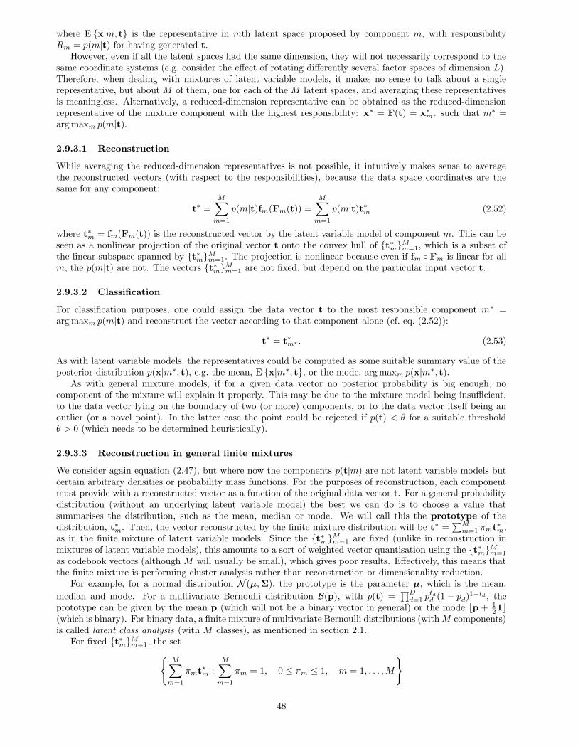
where E {x|m, t} is the representative in mth latent space proposed by component m, with responsibilityRm = p(m|t) for having generated t.

However, even if all the latent spaces had the same dimension, they will not necessarily correspond to thesame coordinate systems (e.g. consider the effect of rotating differently several factor spaces of dimension L).Therefore, when dealing with mixtures of latent variable models, it makes no sense to talk about a singlerepresentative, but about M of them, one for each of the M latent spaces, and averaging these representativesis meaningless. Alternatively, a reduced-dimension representative can be obtained as the reduced-dimensionrepresentative of the mixture component with the highest responsibility: x∗ = F(t) = x∗

m∗ such that m∗ =arg maxm p(m|t).

2.9.3.1 Reconstruction

While averaging the reduced-dimension representatives is not possible, it intuitively makes sense to averagethe reconstructed vectors (with respect to the responsibilities), because the data space coordinates are thesame for any component:

t∗ =M∑

m=1

p(m|t)fm(Fm(t)) =M∑

m=1

p(m|t)t∗m (2.52)

where t∗m = fm(Fm(t)) is the reconstructed vector by the latent variable model of component m. This can beseen as a nonlinear projection of the original vector t onto the convex hull of {t∗m}Mm=1, which is a subset ofthe linear subspace spanned by {t∗m}Mm=1. The projection is nonlinear because even if fm ◦Fm is linear for allm, the p(m|t) are not. The vectors {t∗m}Mm=1 are not fixed, but depend on the particular input vector t.

2.9.3.2 Classification

For classification purposes, one could assign the data vector t to the most responsible component m∗ =arg maxm p(m|t) and reconstruct the vector according to that component alone (cf. eq. (2.52)):

t∗ = t∗m∗ . (2.53)

As with latent variable models, the representatives could be computed as some suitable summary value of theposterior distribution p(x|m∗, t), e.g. the mean, E {x|m∗, t}, or the mode, arg maxm p(x|m∗, t).

As with general mixture models, if for a given data vector no posterior probability is big enough, nocomponent of the mixture will explain it properly. This may be due to the mixture model being insufficient,to the data vector lying on the boundary of two (or more) components, or to the data vector itself being anoutlier (or a novel point). In the latter case the point could be rejected if p(t) < θ for a suitable thresholdθ > 0 (which needs to be determined heuristically).

2.9.3.3 Reconstruction in general finite mixtures

We consider again equation (2.47), but where now the components p(t|m) are not latent variable models butcertain arbitrary densities or probability mass functions. For the purposes of reconstruction, each componentmust provide with a reconstructed vector as a function of the original data vector t. For a general probabilitydistribution (without an underlying latent variable model) the best we can do is to choose a value thatsummarises the distribution, such as the mean, median or mode. We will call this the prototype of thedistribution, t∗m. Then, the vector reconstructed by the finite mixture distribution will be t∗ =

∑Mm=1 πmt∗m,

as in the finite mixture of latent variable models. Since the {t∗m}Mm=1 are fixed (unlike in reconstruction inmixtures of latent variable models), this amounts to a sort of weighted vector quantisation using the {t∗m}Mm=1

as codebook vectors (although M will usually be small), which gives poor results. Effectively, this means thatthe finite mixture is performing cluster analysis rather than reconstruction or dimensionality reduction.

For example, for a normal distribution N (µ,Σ), the prototype is the parameter µ, which is the mean,

median and mode. For a multivariate Bernoulli distribution B(p), with p(t) =∏Dd=1 p

tdd (1− pd)1−td , the

prototype can be given by the mean p (which will not be a binary vector in general) or the mode bp + 121c

(which is binary). For binary data, a finite mixture of multivariate Bernoulli distributions (withM components)is called latent class analysis (with M classes), as mentioned in section 2.1.

For fixed {t∗m}Mm=1, the set

{M∑

m=1

πmt∗m :

M∑

m=1

πm = 1, 0 ≤ πm ≤ 1, m = 1, . . . ,M

}

48

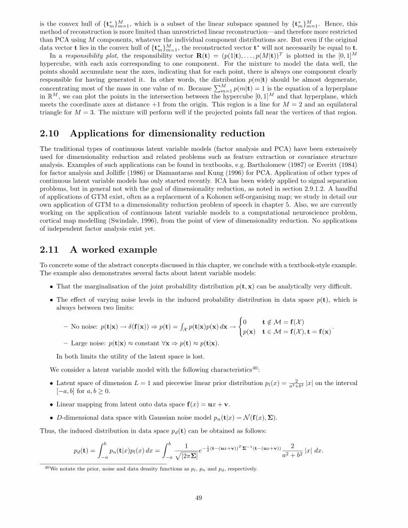
is the convex hull of {t∗m}Mm=1, which is a subset of the linear subspace spanned by {t∗m}Mm=1. Hence, thismethod of reconstruction is more limited than unrestricted linear reconstruction—and therefore more restrictedthan PCA using M components, whatever the individual component distributions are. But even if the originaldata vector t lies in the convex hull of {t∗m}Mm=1, the reconstructed vector t∗ will not necessarily be equal to t.

In a responsibility plot, the responsibility vector R(t) = (p(1|t), . . . , p(M |t))T is plotted in the [0, 1]M

hypercube, with each axis corresponding to one component. For the mixture to model the data well, thepoints should accumulate near the axes, indicating that for each point, there is always one component clearlyresponsible for having generated it. In other words, the distribution p(m|t) should be almost degenerate,

concentrating most of the mass in one value of m. Because∑Mm=1 p(m|t) = 1 is the equation of a hyperplane

in RM , we can plot the points in the intersection between the hypercube [0, 1]M and that hyperplane, whichmeets the coordinate axes at distance +1 from the origin. This region is a line for M = 2 and an equilateraltriangle for M = 3. The mixture will perform well if the projected points fall near the vertices of that region.

2.10 Applications for dimensionality reduction

The traditional types of continuous latent variable models (factor analysis and PCA) have been extensivelyused for dimensionality reduction and related problems such as feature extraction or covariance structureanalysis. Examples of such applications can be found in textbooks, e.g. Bartholomew (1987) or Everitt (1984)for factor analysis and Jolliffe (1986) or Diamantaras and Kung (1996) for PCA. Application of other types ofcontinuous latent variable models has only started recently. ICA has been widely applied to signal separationproblems, but in general not with the goal of dimensionality reduction, as noted in section 2.9.1.2. A handfulof applications of GTM exist, often as a replacement of a Kohonen self-organising map; we study in detail ourown application of GTM to a dimensionality reduction problem of speech in chapter 5. Also, we are currentlyworking on the application of continuous latent variable models to a computational neuroscience problem,cortical map modelling (Swindale, 1996), from the point of view of dimensionality reduction. No applicationsof independent factor analysis exist yet.

2.11 A worked example

To concrete some of the abstract concepts discussed in this chapter, we conclude with a textbook-style example.The example also demonstrates several facts about latent variable models:

• That the marginalisation of the joint probability distribution p(t,x) can be analytically very difficult.

• The effect of varying noise levels in the induced probability distribution in data space p(t), which isalways between two limits:

– No noise: p(t|x)→ δ(f(x))⇒ p(t) =∫

X p(t|x)p(x) dx→{

0 t /∈M = f(X )

p(x) t ∈M = f(X ), t = f(x).

– Large noise: p(t|x) ≈ constant ∀x⇒ p(t) ≈ p(t|x).

In both limits the utility of the latent space is lost.

We consider a latent variable model with the following characteristics40:

• Latent space of dimension L = 1 and piecewise linear prior distribution pl(x) = 2a2+b2 |x| on the interval

[−a, b] for a, b ≥ 0.

• Linear mapping from latent onto data space f(x) = ux+ v.

• D-dimensional data space with Gaussian noise model pn(t|x) = N (f(x),Σ).

Thus, the induced distribution in data space pd(t) can be obtained as follows:

pd(t) =

∫ b

−apn(t|x)pl(x) dx =

∫ b

−a

1√

|2πΣ|e−

12 (t−(ux+v))T Σ−1(t−(ux+v)) 2

a2 + b2|x| dx.

40We notate the prior, noise and data density functions as pl, pn and pd, respectively.

49

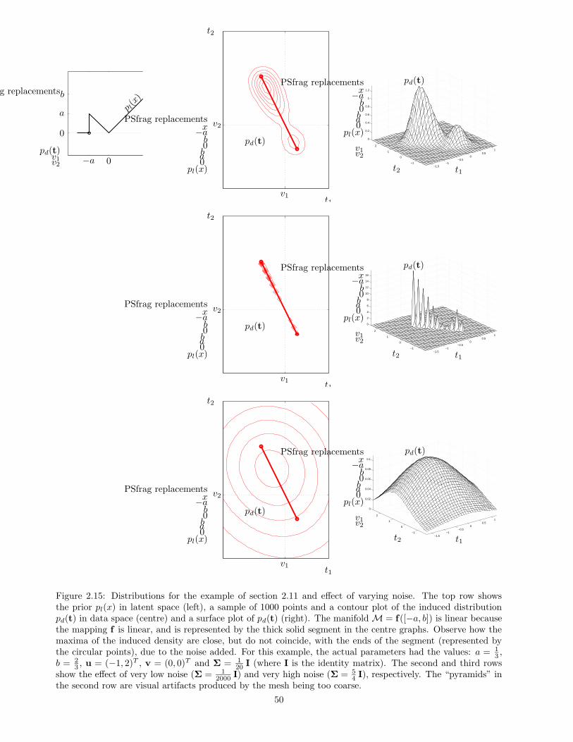
PSfrag replacements

x−a b0

b

a

0

p l(x

)

pd(t)v1v2

PSfrag replacementsx−ab0ba0

pl(x)

pd(t)

v1

v2

t1

t2

−1.5−1

−0.50

0.51

−1

0

1

2

0

0.2

0.4

0.6

0.8

1

1.2

PSfrag replacementsx−ab0ba0

pl(x)

pd(t)

v1v2

t1t2

PSfrag replacementsx−ab0ba0

pl(x)

pd(t)

v1

v2

t1

t2

−1.5−1

−0.50

0.51

−1

0

1

2

0

2

4

6

8

10

12

14

16

PSfrag replacementsx−ab0ba0

pl(x)

pd(t)

v1v2

t1t2

PSfrag replacementsx−ab0ba0

pl(x)

pd(t)

v1

v2

t1

t2

−1.5−1

−0.50

0.51

−1

0

1

2

0

0.02

0.04

0.06

0.08

0.1

PSfrag replacementsx−ab0ba0

pl(x)

pd(t)

v1v2

t1t2

Figure 2.15: Distributions for the example of section 2.11 and effect of varying noise. The top row showsthe prior pl(x) in latent space (left), a sample of 1000 points and a contour plot of the induced distributionpd(t) in data space (centre) and a surface plot of pd(t) (right). The manifoldM = f([−a, b]) is linear becausethe mapping f is linear, and is represented by the thick solid segment in the centre graphs. Observe how themaxima of the induced density are close, but do not coincide, with the ends of the segment (represented bythe circular points), due to the noise added. For this example, the actual parameters had the values: a = 1

3 ,b = 2

3 , u = (−1, 2)T , v = (0, 0)T and Σ = 120 I (where I is the identity matrix). The second and third rows

show the effect of very low noise (Σ = 12000 I) and very high noise (Σ = 5

4 I), respectively. The “pyramids” inthe second row are visual artifacts produced by the mesh being too coarse.

50

PSfrag replacements

t1

t2

pd(t)

v1

v2

PSfrag replacements

t1

t2

pd(t)

v1

v2

PSfrag replacements

t1

t2

pd(t)

v1

v2

Figure 2.16: Models for the example of section 2.11 (from left to right): factor analysis (L = 1 factor),principal component analysis (L = 1 principal component) and GTM (K = 11 latent grid points, F = 5 radialbasis functions with a standard deviation s = 1 times their separation, EM starting point: the line of thefirst principal component). For each model, the thick dashed line corresponds to the manifoldM = f([−a, b])(which in GTM’s case overlaps the true one, represented by the thick solid segment). The grey circles in GTM’sgraph represent the K Gaussian components associated to the latent grid points (eqs. (2.42) and (2.43), witha radius σ). The training set contained N = 10 000 points.

Changing variables to A = uTΣ−1u, B = −2(t−v)TΣ−1u, C = (t−v)TΣ−1(t−v), m = −B2A and σ = A−1/2

we obtain:

pd(t) =2

a2 + b21

√

|2πΣ|

∫ b

−a|x| e− 1

2 (Ax2+Bx+C) dx =2

a2 + b21

√

|2πΣ|

∫ b

−a|x| e−

12

[

( x−mσ )

2+(m

σ )2−C

]

dx

and, changing again to α = a+mσ√

2, β = b−m

σ√

2and γ = m

σ√

2, we finally obtain:

pd(t) =2

a2 + b2σ2

√

|2πΣ|eγ

2−C2

{

−e−α2 − e−β2

+ 2e−γ2

+ γ√π (erf(β)− erf(α) + 2 erf(γ))

}

,

where erf(x) = 2√π

∫ x

0e−t

2

dt is the error function, which does not have a closed-form expression. α, β and γ

are functions of t and σ depends on the noise and mapping but not on t.Figure 2.15 shows the prior in latent space pl(x) and the induced distribution in data space pd(t) for the

true distribution, as well as the effects of low and high noise. Figure 2.16 shows the data space distributionfor factor analysis, principal component analysis and GTM. Figure 2.17 comparatively shows the distributionin data space along the manifold segment.

Even though for this problem the true manifold in data space is linear, the distribution pd(t) in dataspace is not normal because the prior distribution pl(x) in latent space is not normal. Thus, the linear-normalmodels (factor analysis and principal component analysis) produce a bad model while GTM models the truedistribution very well. It is interesting to observe that both factor analysis and PCA produce exactly the samenormal distribution pd(t), but while the PCA manifold MPCA is aligned with the Gaussian’s principal axis,the factor analysis manifold MFA is not. The reasons are:

• In this example, whereD = 2 and L = 1, the number of free parameters for factor analysis is D(L+1) = 4and for principal component analysis DL+1 = 3. Since the covariance matrix of a bidimensional normal

distribution is determined by only D(D+1)2 = 3 parameters, both models will account exactly for (and

coincide with) the sample covariance matrix—which is the best they can do. Furthermore, since thefactor analysis model has more parameters than needed—rotation constraints are not possible becausethe latent space is one-dimensional—it is undertermined (i.e., non-identifiable): there is an infinitenumber of equivalent combinations for the values of Λ and Ψ (one of them being the PCA solution).

• For factor analysis, the uniqueness matrix Ψ is not isotropic in general (except when it coincides with thePCA solution), as happens for the maximum likelihood estimate found in fig. 2.16, where ψ1 < ψ2. Thus

51

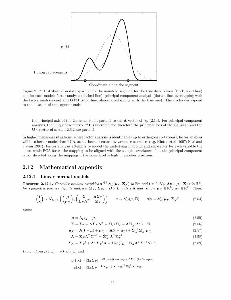
PSfrag replacements

pd(t)

Coordinate along the segment

Figure 2.17: Distribution in data space along the manifold segment for the true distribution (thick, solid line)and for each model: factor analysis (dashed line), principal component analysis (dotted line, overlapping withthe factor analysis one) and GTM (solid line, almost overlapping with the true one). The circles correspondto the location of the segment ends.

the principal axis of the Gaussian is not parallel to the Λ vector of eq. (2.14). For principal componentanalysis, the uniqueness matrix σ2I is isotropic and therefore the principal axis of the Gaussian and theUL vector of section 2.6.2 are parallel.

In high-dimensional situations, where factor analysis is identifiable (up to orthogonal rotations), factor analysiswill be a better model than PCA, as has been discussed by various researchers (e.g. Hinton et al. 1997; Neal andDayan 1997). Factor analysis attempts to model the underlying mapping and separately for each variable thenoise, while PCA forces the mapping to be aligned with the sample covariance—but the principal componentis not directed along the mapping if the noise level is high in another direction.

2.12 Mathematical appendix

2.12.1 Linear-normal models

Theorem 2.12.1. Consider random variables xdef∼ NL(µX ,ΣX) in RL and t|x def∼ ND(Λx + µT ,ΣT ) in RD,

for symmetric positive definite matrices ΣX , ΣT , a D × L matrix Λ and vectors µX ∈ RL, µT ∈ RD. Then:

(tx

)

∼ ND+L

((µ

µX

)

,

(Σ ΛΣX

ΣXΛT ΣX

))

t ∼ ND(µ,Σ) x|t ∼ NL(µX , Σ−1X ) (2.54)

where

µ = ΛµX + µT (2.55)

Σ = ΣT + ΛΣXΛT = ΣT (ΣT −ΛΣ−1X ΛT )−1ΣT (2.56)

µX = A(t− µ) + µX = A(t− µT ) + Σ−1X Σ−1

X µX (2.57)

A = ΣXΛTΣ−1 = Σ−1X ΛTΣ−1

T (2.58)

ΣX = Σ−1X + ΛTΣ−1

T Λ = Σ−1X (IL −ΣXΛTΣ−1Λ)−1. (2.59)

Proof. From p(t,x) = p(t|x)p(x) and

p(t|x) = |2πΣT |−1/2e−

12 (t−Λx−µT )T Σ

−1T (t−Λx−µT )

p(x) = |2πΣX |−1/2e−

12 (x−µX)T Σ

−1X (x−µX)

52

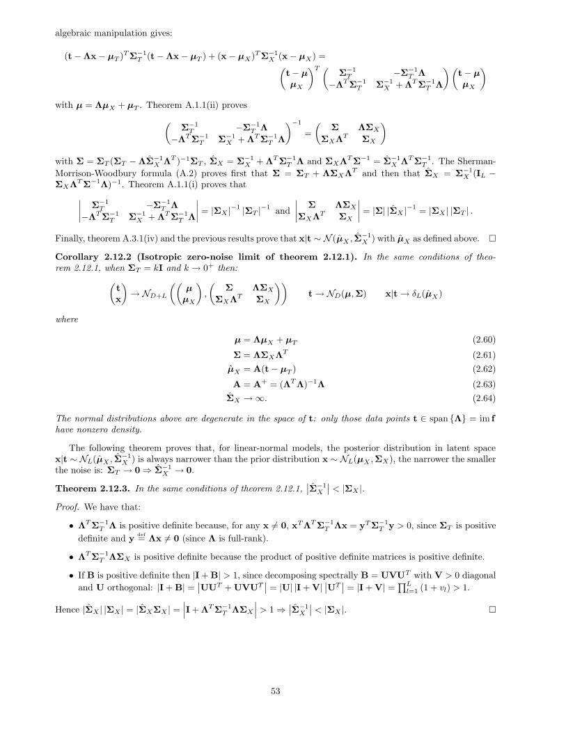
algebraic manipulation gives:

(t−Λx− µT )TΣ−1T (t−Λx− µT ) + (x− µX)TΣ−1

X (x− µX) =(t− µ

µX

)T (Σ−1T −Σ−1

T Λ

−ΛTΣ−1T Σ−1

X + ΛTΣ−1T Λ

)(t− µ

µX

)

with µ = ΛµX + µT . Theorem A.1.1(ii) proves

(Σ−1T −Σ−1

T Λ

−ΛTΣ−1T Σ−1

X + ΛTΣ−1T Λ

)−1

=

(Σ ΛΣX

ΣXΛT ΣX

)

with Σ = ΣT (ΣT −ΛΣ−1X ΛT )−1ΣT , ΣX = Σ−1

X + ΛTΣ−1T Λ and ΣXΛTΣ−1 = Σ−1

X ΛTΣ−1T . The Sherman-

Morrison-Woodbury formula (A.2) proves first that Σ = ΣT + ΛΣXΛT and then that ΣX = Σ−1X (IL −

ΣXΛTΣ−1Λ)−1. Theorem A.1.1(i) proves that

∣∣∣∣

Σ−1T −Σ−1

T Λ

−ΛTΣ−1T Σ−1

X + ΛTΣ−1T Λ

∣∣∣∣= |ΣX |−1 |ΣT |−1

and

∣∣∣∣

Σ ΛΣX

ΣXΛT ΣX

∣∣∣∣= |Σ| |ΣX |−1

= |ΣX | |ΣT | .

Finally, theorem A.3.1(iv) and the previous results prove that x|t ∼ N (µX , Σ−1X ) with µX as defined above.

Corollary 2.12.2 (Isotropic zero-noise limit of theorem 2.12.1). In the same conditions of theo-rem 2.12.1, when ΣT = kI and k → 0+ then:

(tx

)

→ ND+L

((µ

µX

)

,

(Σ ΛΣX

ΣXΛT ΣX

))

t→ ND(µ,Σ) x|t→ δL(µX)

where

µ = ΛµX + µT (2.60)

Σ = ΛΣXΛT (2.61)

µX = A(t− µT ) (2.62)

A = A+ = (ΛTΛ)−1Λ (2.63)

ΣX →∞. (2.64)

The normal distributions above are degenerate in the space of t: only those data points t ∈ span {Λ} = im fhave nonzero density.

The following theorem proves that, for linear-normal models, the posterior distribution in latent spacex|t ∼ NL(µX , Σ

−1X ) is always narrower than the prior distribution x ∼ NL(µX ,ΣX), the narrower the smaller

the noise is: ΣT → 0⇒ Σ−1X → 0.

Theorem 2.12.3. In the same conditions of theorem 2.12.1,∣∣Σ−1

X

∣∣ < |ΣX |.

Proof. We have that:

• ΛTΣ−1T Λ is positive definite because, for any x 6= 0, xTΛTΣ−1

T Λx = yTΣ−1T y > 0, since ΣT is positive

definite and ydef= Λx 6= 0 (since Λ is full-rank).

• ΛTΣ−1T ΛΣX is positive definite because the product of positive definite matrices is positive definite.

• If B is positive definite then |I + B| > 1, since decomposing spectrally B = UVUT with V > 0 diagonal

and U orthogonal: |I + B| =∣∣UUT + UVUT

∣∣ = |U| |I + V|

∣∣UT

∣∣ = |I + V| = ∏L

l=1 (1 + vl) > 1.

Hence |ΣX | |ΣX | = |ΣXΣX | =∣∣∣I + ΛTΣ−1

T ΛΣX

∣∣∣ > 1⇒

∣∣Σ−1

X

∣∣ < |ΣX |.

53

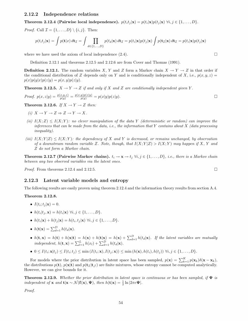
2.12.2 Independence relations

Theorem 2.12.4 (Pairwise local independence). p(titj |x) = p(ti|x)p(tj |x) ∀i, j ∈ {1, . . . , D}.

Proof. Call I = {1, . . . , D} \ {i, j}. Then:

p(titj |x) =

∫

p(t|x) dtI =

∫∏

d∈{1,...,D}p(td|x) dtI = p(ti|x)p(tj |x)

∫

p(tI |x) dtI = p(ti|x)p(tj |x)

where we have used the axiom of local independence (2.4).

Definition 2.12.1 and theorems 2.12.5 and 2.12.6 are from Cover and Thomas (1991).

Definition 2.12.1. The random variables X, Y and Z form a Markov chain X → Y → Z in that order ifthe conditional distribution of Z depends only on Y and is conditionally independent of X, i.e., p(x, y, z) =p(x)p(y|x)p(z|y) = p(x, y)p(z|y).

Theorem 2.12.5. X → Y → Z if and only if X and Z are conditionally independent given Y .

Proof. p(x, z|y) = p(x,y,z)p(y) = p(x,y)p(z|y)

p(y) = p(x|y)p(z|y).

Theorem 2.12.6. If X → Y → Z then:

(i) X → Y → Z ⇒ Z → Y → X.

(ii) I(X;Z) ≤ I(X;Y ): no clever manipulation of the data Y (deterministic or random) can improve theinferences that can be made from the data, i.e., the information that Y contains about X (data processinginequality).

(iii) I(X;Y |Z) ≤ I(X;Y ): the dependency of X and Y is decreased, or remains unchanged, by observationof a downstream random variable Z. Note, though, that I(X;Y |Z) > I(X;Y ) may happen if X, Y andZ do not form a Markov chain.

Theorem 2.12.7 (Pairwise Markov chains). ti → x→ tj ∀i, j ∈ {1, . . . , D}, i.e., there is a Markov chainbetween any two observed variables via the latent ones.

Proof. From theorems 2.12.4 and 2.12.5.

2.12.3 Latent variable models and entropy

The following results are easily proven using theorem 2.12.4 and the information theory results from section A.4.

Theorem 2.12.8.

• I(ti; tj |x) = 0.

• h(ti|tj ,x) = h(ti|x) ∀i, j ∈ {1, . . . , D}.

• h(ti|x) + h(tj |x) = h(ti, tj |x) ∀i, j ∈ {1, . . . , D}.

• h(t|x) =∑Dd=1 h(td|x).

• h(t,x) = h(t) + h(x|t) = h(x) + h(t|x) = h(x) +∑Dd=1 h(td|x). If the latent variables are mutually

independent, h(t,x) =∑Ll=1 h(xl) +

∑Dd=1 h(td|x).

• 0 ≤ I(ti;x|tj) ≤ I(ti; tj) ≤ min (I(ti;x), I(tj ;x)) ≤ min (h(x), h(ti), h(tj)) ∀i, j ∈ {1, . . . , D}.

For models where the prior distribution in latent space has been sampled, p(x) =∑Kk=1 p(xk)δ(x− xk),

the distributions p(t), p(x|t) and p(tI |tJ ) are finite mixtures, whose entropy cannot be computed analytically.However, we can give bounds for it.

Theorem 2.12.9. Whether the prior distribution in latent space is continuous or has been sampled, if Ψ isindependent of x and t|x ∼ N (f(x),Ψ), then h(t|x) = 1

2 ln |2πeΨ|.

Proof.

54

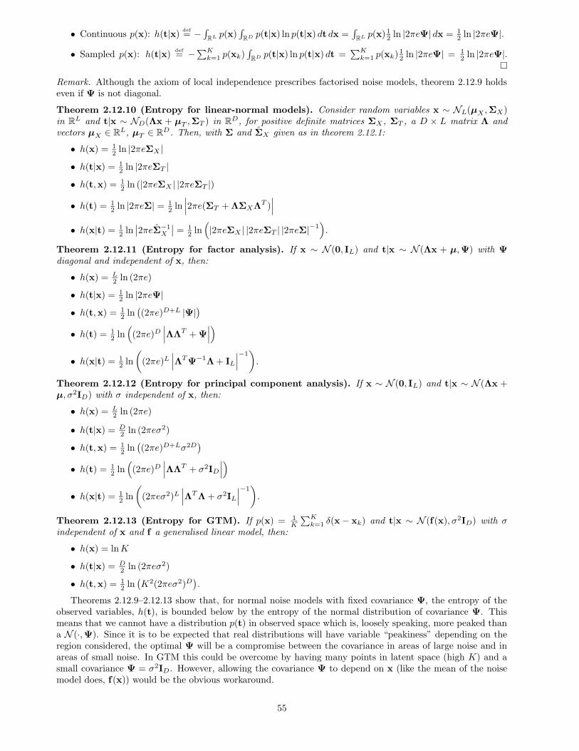
• Continuous p(x): h(t|x)def= −

∫

RL p(x)∫

RD p(t|x) ln p(t|x) dt dx =∫

RL p(x) 12 ln |2πeΨ| dx = 1

2 ln |2πeΨ|.

• Sampled p(x): h(t|x)def= −∑K

k=1 p(xk)∫

RD p(t|x) ln p(t|x) dt =∑Kk=1 p(xk)

12 ln |2πeΨ| = 1

2 ln |2πeΨ|.

Remark. Although the axiom of local independence prescribes factorised noise models, theorem 2.12.9 holdseven if Ψ is not diagonal.

Theorem 2.12.10 (Entropy for linear-normal models). Consider random variables x ∼ NL(µX ,ΣX)in RL and t|x ∼ ND(Λx + µT ,ΣT ) in RD, for positive definite matrices ΣX , ΣT , a D × L matrix Λ andvectors µX ∈ RL, µT ∈ RD. Then, with Σ and ΣX given as in theorem 2.12.1:

• h(x) = 12 ln |2πeΣX |

• h(t|x) = 12 ln |2πeΣT |

• h(t,x) = 12 ln (|2πeΣX | |2πeΣT |)

• h(t) = 12 ln |2πeΣ| = 1

2 ln∣∣∣2πe(ΣT + ΛΣXΛT )

∣∣∣

• h(x|t) = 12 ln

∣∣2πeΣ−1

X

∣∣ = 1

2 ln(

|2πeΣX | |2πeΣT | |2πeΣ|−1)

.

Theorem 2.12.11 (Entropy for factor analysis). If x ∼ N (0, IL) and t|x ∼ N (Λx + µ,Ψ) with Ψdiagonal and independent of x, then:

• h(x) = L2 ln (2πe)

• h(t|x) = 12 ln |2πeΨ|

• h(t,x) = 12 ln

((2πe)D+L |Ψ|

)

• h(t) = 12 ln

(

(2πe)D∣∣∣ΛΛT + Ψ

∣∣∣

)

• h(x|t) = 12 ln

(

(2πe)L∣∣∣ΛTΨ−1Λ + IL

∣∣∣

−1)

.

Theorem 2.12.12 (Entropy for principal component analysis). If x ∼ N (0, IL) and t|x ∼ N (Λx +µ, σ2ID) with σ independent of x, then:

• h(x) = L2 ln (2πe)

• h(t|x) = D2 ln (2πeσ2)

• h(t,x) = 12 ln

((2πe)D+Lσ2D

)

• h(t) = 12 ln

(

(2πe)D∣∣∣ΛΛT + σ2ID

∣∣∣

)

• h(x|t) = 12 ln

(

(2πeσ2)L∣∣∣ΛTΛ + σ2IL

∣∣∣

−1)

.

Theorem 2.12.13 (Entropy for GTM). If p(x) = 1K

∑Kk=1 δ(x− xk) and t|x ∼ N (f(x), σ2ID) with σ

independent of x and f a generalised linear model, then:

• h(x) = lnK

• h(t|x) = D2 ln (2πeσ2)

• h(t,x) = 12 ln

(K2(2πeσ2)D

).

Theorems 2.12.9–2.12.13 show that, for normal noise models with fixed covariance Ψ, the entropy of theobserved variables, h(t), is bounded below by the entropy of the normal distribution of covariance Ψ. Thismeans that we cannot have a distribution p(t) in observed space which is, loosely speaking, more peaked thana N (·,Ψ). Since it is to be expected that real distributions will have variable “peakiness” depending on theregion considered, the optimal Ψ will be a compromise between the covariance in areas of large noise and inareas of small noise. In GTM this could be overcome by having many points in latent space (high K) and asmall covariance Ψ = σ2ID. However, allowing the covariance Ψ to depend on x (like the mean of the noisemodel does, f(x)) would be the obvious workaround.

55

2.12.4 Diagonal GTM (dGTM)

We give here the details for dGTM, the diagonal noise model for GTM that we proposed in section 2.6.5.1.First let us fully generalise GTM so that it has diagonal noise dependent on each latent grid point and boththe values of the noise covariance matrix and the values of the prior distribution in latent space are trainable.Thus

t|x def∼ N (f(x),Ψ(x)) (2.42’)

with Ψ : X → (R+)D and

p(t) =K∑

k=1

πkp(t|xk)

with πkdef= p(xk) and Ψk

def= Ψ(xk) = diag (ψk1, . . . , ψkD). The dependence of p(t|xk) on all the relevant

parameters is not explicitly written for clarity of notation. The EM equations are derived by minimising

N∑

n=1

ln p(tn)− λ(

K∑

k=1

πk − 1

)

where λ is a Lagrange multiplier that ensures that the values of the prior distribution in latent space add toone. This gives

π(τ+1)k =

1

N

N∑

n=1

p(xk|tn) =1

N

N∑

n=1

R(τ)nk

for the prior distribution in latent space, using the responsibilities Rnk = p(xk|tn), and for the rest of theparameters we obtain

N∑

n=1

K∑

k=1

Rnk∂

∂θln p(tn|xk) = 0 (2.65)

where θ represents a parameter wdf or ψkd. Recalling that fd(xk) =∑Ff=1 wdfφkf where φkf = φf (xk) and

plugging

∂

∂wdfln p(tn|xk) =

φkfψkd

tnd −F∑

f ′=1

wdf ′φkf ′

d = 1, . . . , D f = 1, . . . , F

∂

∂ψkdln p(tn|xk) = −1

2

(1

ψkd− (tnd − fd(xk))2

ψ2kd

)

k = 1, . . . ,K d = 1, . . . , D

∂

∂ψkdln p(tn|xk′) = 0 if k 6= k′

into (2.65), we obtain a system of D(F +K) equations that, together with the equations for {πk}Kk=1, definethe M step:

K∑

k=1

φkfψkd

gkk

F∑

f ′=1

φkf ′wdf ′ =N∑

n=1

K∑

k=1

φkfψkd

Rnktnd d = 1, . . . , D f = 1, . . . , F

ψkd =1

gkk

N∑

n=1

Rnk(tnd − fd(xk))2 k = 1, . . . ,K d = 1, . . . , D

where gkkdef=∑Nn=1Rnk as in section 2.6.5. Solving for {wdf}D,Fd,f=1 is cumbersome, since the first group of

equations cannot be put into a nice matrix equation form. The second group of equations shows that Ψk is aweighted average of the squared componentwise deviations of the data points from the “reference point” f(xk),where the weights are given by the responsibilities (normalised over all reference points).

Compared to the standard GTM model, this extended version has K(D+1)−2 more parameters: {πk}K−1k=1

and {Ψk}Kk=1. Thus, we lose the attractive property that using a large number of latent pointsK (exponentiallydependent on the latent space dimension L) does not increase the number of parameters. Even if the EMalgorithm was straightforward, such a model would require a large training set for stable statistical estimation41

41Note, however, that the standard GTM model does depend on F , the number of radial basis functions needed for the mappingf , which also depends exponentially on L (but can be kept quite smaller than K without losing approximation power).

56

and would be prone to singularity problems (Ψk → 0 for some k), as mentioned in section 2.5.2, among otherplaces. Defining Ψ(x) as a generalised linear model (as f is, eq. (2.41), and reusing the φ function) eliminatesthe direct dependence on K and ensures a smooth variability of the noise variance over the data manifold, butthe resulting M step is unsolvable, as can be readily checked. Also, since f is a universal approximator, it isnot really necessary to make the prior distribution in latent space trainable as well.

Taking into account these considerations, for all k = 1, . . . ,K we keep p(xk) = 1K constant as in the

standard GTM model and the noise model covariance matrix Ψk = Ψ diagonal constant too. As can easily beseen by recalculating ∂

∂ψdln p(tn|xk), the M step becomes exactly solvable and leads to the following update

equations for the parameters W and Ψ, respectively:

ΦTG(τ)Φ(W(τ+1))T = ΦT (R(τ))TT (2.45a)

ψ(τ+1)d =

1

N

K∑

k=1

N∑

n=1

R(τ)nk (tnd − fd(xk))2 d = 1, . . . , D (2.45b’)

the first of which is the same one as for the standard GTM model and the second of which has the sameinterpretation as before as weighted average of the squared componentwise deviations of the data points fromf(xk). Further modifications can still be done, such as a Gaussian regularisation term on W, eq. (2.46), or aunit-speed constraint on f , section 2.8.3.

❦

57

Bibliography

S. Amari. Natural gradient learning for over- and under-complete bases in ICA. Neural Computation, 11(8):1875–1883, Nov. 1999.

S. Amari and A. Cichoki. Adaptive blind signal processing—neural network approaches. Proc. IEEE, 86(10):2026–2048, Oct. 1998.

T. W. Anderson. Asymptotic theory for principal component analysis. Annals of Mathematical Statistics, 34(1):122–148, Mar. 1963.

T. W. Anderson and H. Rubin. Statistical inference in factor analysis. In J. Neyman, editor, Proc. 3rdBerkeley Symp. Mathematical Statistics and Probability, volume V, pages 111–150, Berkeley, 1956. Universityof California Press.

S. Arnfield. Artificial EPG palate image. The Reading EPG, 1995. Available online at http://www.

linguistics.reading.ac.uk/research/speechlab/epg/palate.jpg, Feb. 1, 2000.

H. Asada and J.-J. E. Slotine. Robot Analysis and Control. John Wiley & Sons, New York, London, Sydney,1986.

D. Asimov. The grand tour: A tool for viewing multidimensional data. SIAM J. Sci. Stat. Comput., 6:128–143,1985.

B. S. Atal, J. J. Chang, M. V. Mathews, and J. W. Tukey. Inversion of articulatory-to-acoustic transformationin the vocal tract by a computer-sorting technique. J. Acoustic Soc. Amer., 63(5):1535–1555, May 1978.

C. G. Atkeson. Learning arm kinematics and dynamics. Annu. Rev. Neurosci., 12:157–183, 1989.

H. Attias. EM algorithms for independent component analysis. In Niranjan (1998), pages 132–141.

H. Attias. Independent factor analysis. Neural Computation, 11(4):803–851, May 1999.

F. Aurenhammer. Voronoi diagrams—a survey of a fundamental geometric data structure. ACM ComputingSurveys, 23(3):345–405, Sept. 1991.

A. Azzalini and A. Capitanio. Statistical applications of the multivariate skew-normal distribution. Journalof the Royal Statistical Society, B, 61(3):579–602, 1999.

R. J. Baddeley. Searching for filters with “interesting” output distributions: An uninteresting direction toexplore? Network: Computation in Neural Systems, 7(2):409–421, 1996.

R. Bakis. Coarticulation modeling with continuous-state HMMs. In Proc. IEEE Workshop Automatic SpeechRecognition, pages 20–21, Arden House, New York, 1991. Harriman.

R. Bakis. An articulatory-like speech production model with controlled use of prior knowledge. Frontiers inSpeech Processing: Robust Speech Analysis ’93, Workshop CDROM, NIST Speech Disc 15 (also availablefrom the Linguistic Data Consortium), Aug. 6 1993.

P. Baldi and K. Hornik. Neural networks and principal component analysis: Learning from examples withoutlocal minima. Neural Networks, 2(1):53–58, 1989.

J. D. Banfield and A. E. Raftery. Ice floe identification in satellite images using mathematical morphologyand clustering about principal curves. J. Amer. Stat. Assoc., 87(417):7–16, Mar. 1992.

294

J. Barker, L. Josifovski, M. Cooke, and P. Green. Soft decisions in missing data techniques for robust automaticspeech recognition. In Proc. of the International Conference on Spoken Language Processing (ICSLP’00),Beijing, China, Oct. 16–20 2000.

J. P. Barker and F. Berthommier. Evidence of correlation between acoustic and visual features of speech. InOhala et al. (1999), pages 199–202.

M. F. Barnsley. Fractals Everywhere. Academic Press, New York, 1988.

D. J. Bartholomew. The foundations of factor analysis. Biometrika, 71(2):221–232, Aug. 1984.

D. J. Bartholomew. Foundations of factor analysis: Some practical implications. Brit. J. of Mathematical andStatistical Psychology, 38:1–10 (discussion in pp. 127–140), 1985.

D. J. Bartholomew. Latent Variable Models and Factor Analysis. Charles Griffin & Company Ltd., London,1987.

A. Basilevsky. Statistical Factor Analysis and Related Methods. Wiley Series in Probability and MathematicalStatistics. John Wiley & Sons, New York, London, Sydney, 1994.

H.-U. Bauer, M. Herrmann, and T. Villmann. Neural maps and topographic vector quantization. NeuralNetworks, 12(4–5):659–676, June 1999.

H.-U. Bauer and K. R. Pawelzik. Quantifying the neighbourhood preservation of self-organizing feature maps.IEEE Trans. Neural Networks, 3(4):570–579, July 1992.

J. Behboodian. On the modes of a mixture of two normal distributions. Technometrics, 12(1):131–139, Feb.1970.

A. J. Bell and T. J. Sejnowski. An information-maximization approach to blind separation and blind decon-volution. Neural Computation, 7(6):1129–1159, 1995.

A. J. Bell and T. J. Sejnowski. The “independent components” of natural scenes are edge filters. Vision Res.,37(23):3327–3338, Dec. 1997.

R. Bellman. Dynamic Programming. Princeton University Press, Princeton, 1957.

R. Bellman. Adaptive Control Processes: A Guided Tour. Princeton University Press, Princeton, 1961.

Y. Bengio and F. Gingras. Recurrent neural networks for missing or asynchronous data. In D. S. Touretzky,M. C. Mozer, and M. E. Hasselmo, editors, Advances in Neural Information Processing Systems, volume 8,pages 395–401. MIT Press, Cambridge, MA, 1996.

C. Benoıt, M.-T. Lallouache, T. Mohamadi, and C. Abry. A set of French visemes for visual speech synthesis.In G. Bailly and C. Benoıt, editors, Talking Machines: Theories, Models and Designs, pages 485–504. NorthHolland-Elsevier Science Publishers, Amsterdam, New York, Oxford, 1992.

P. M. Bentler and J. S. Tanaka. Problems with EM algorithms for ML factor analysis. Psychometrika, 48(2):247–251, June 1983.

J. O. Berger. Statistical Decision Theory and Bayesian Analysis. Springer Series in Statistics. Springer-Verlag,Berlin, second edition, 1985.

M. Berkane, editor. Latent Variable Modeling and Applications to Causality. Number 120 in Springer Seriesin Statistics. Springer-Verlag, Berlin, 1997.

J. M. Bernardo and A. F. M. Smith. Bayesian Theory. Wiley Series in Probability and Mathematical Statistics.John Wiley & Sons, Chichester, 1994.

N. Bernstein. The Coordination and Regulation of Movements. Pergamon, Oxford, 1967.

D. P. Bertsekas. Dynamic Programming. Deterministic and Stochastic Models. Prentice-Hall, Englewood Cliffs,N.J., 1987.

J. Besag and P. J. Green. Spatial statistics and Bayesian computation. Journal of the Royal Statistical Society,B, 55(1):25–37, 1993.

295

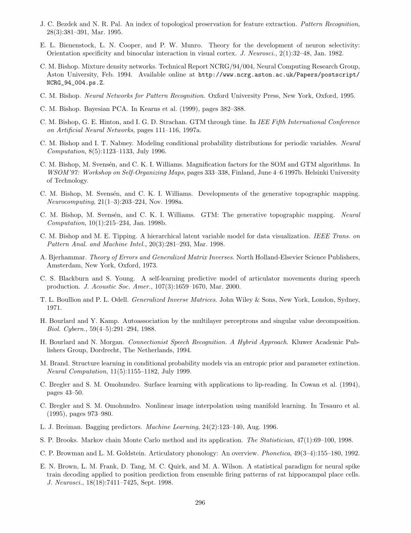
J. C. Bezdek and N. R. Pal. An index of topological preservation for feature extraction. Pattern Recognition,28(3):381–391, Mar. 1995.

E. L. Bienenstock, L. N. Cooper, and P. W. Munro. Theory for the development of neuron selectivity:Orientation specificity and binocular interaction in visual cortex. J. Neurosci., 2(1):32–48, Jan. 1982.

C. M. Bishop. Mixture density networks. Technical Report NCRG/94/004, Neural Computing Research Group,Aston University, Feb. 1994. Available online at http://www.ncrg.aston.ac.uk/Papers/postscript/

NCRG_94_004.ps.Z.

C. M. Bishop. Neural Networks for Pattern Recognition. Oxford University Press, New York, Oxford, 1995.

C. M. Bishop. Bayesian PCA. In Kearns et al. (1999), pages 382–388.

C. M. Bishop, G. E. Hinton, and I. G. D. Strachan. GTM through time. In IEE Fifth International Conferenceon Artificial Neural Networks, pages 111–116, 1997a.

C. M. Bishop and I. T. Nabney. Modeling conditional probability distributions for periodic variables. NeuralComputation, 8(5):1123–1133, July 1996.

C. M. Bishop, M. Svensen, and C. K. I. Williams. Magnification factors for the SOM and GTM algorithms. InWSOM’97: Workshop on Self-Organizing Maps, pages 333–338, Finland, June 4–6 1997b. Helsinki Universityof Technology.

C. M. Bishop, M. Svensen, and C. K. I. Williams. Developments of the generative topographic mapping.Neurocomputing, 21(1–3):203–224, Nov. 1998a.

C. M. Bishop, M. Svensen, and C. K. I. Williams. GTM: The generative topographic mapping. NeuralComputation, 10(1):215–234, Jan. 1998b.

C. M. Bishop and M. E. Tipping. A hierarchical latent variable model for data visualization. IEEE Trans. onPattern Anal. and Machine Intel., 20(3):281–293, Mar. 1998.

A. Bjerhammar. Theory of Errors and Generalized Matrix Inverses. North Holland-Elsevier Science Publishers,Amsterdam, New York, Oxford, 1973.

C. S. Blackburn and S. Young. A self-learning predictive model of articulator movements during speechproduction. J. Acoustic Soc. Amer., 107(3):1659–1670, Mar. 2000.

T. L. Boullion and P. L. Odell. Generalized Inverse Matrices. John Wiley & Sons, New York, London, Sydney,1971.

H. Bourlard and Y. Kamp. Autoassociation by the multilayer perceptrons and singular value decomposition.Biol. Cybern., 59(4–5):291–294, 1988.

H. Bourlard and N. Morgan. Connectionist Speech Recognition. A Hybrid Approach. Kluwer Academic Pub-lishers Group, Dordrecht, The Netherlands, 1994.

M. Brand. Structure learning in conditional probability models via an entropic prior and parameter extinction.Neural Computation, 11(5):1155–1182, July 1999.

C. Bregler and S. M. Omohundro. Surface learning with applications to lip-reading. In Cowan et al. (1994),pages 43–50.

C. Bregler and S. M. Omohundro. Nonlinear image interpolation using manifold learning. In Tesauro et al.(1995), pages 973–980.

L. J. Breiman. Bagging predictors. Machine Learning, 24(2):123–140, Aug. 1996.

S. P. Brooks. Markov chain Monte Carlo method and its application. The Statistician, 47(1):69–100, 1998.

C. P. Browman and L. M. Goldstein. Articulatory phonology: An overview. Phonetica, 49(3–4):155–180, 1992.

E. N. Brown, L. M. Frank, D. Tang, M. C. Quirk, and M. A. Wilson. A statistical paradigm for neural spiketrain decoding applied to position prediction from ensemble firing patterns of rat hippocampal place cells.J. Neurosci., 18(18):7411–7425, Sept. 1998.

296

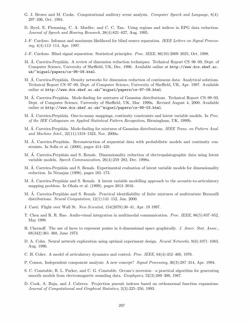
G. J. Brown and M. Cooke. Computational auditory scene analysis. Computer Speech and Language, 8(4):297–336, Oct. 1994.

D. Byrd, E. Flemming, C. A. Mueller, and C. C. Tan. Using regions and indices in EPG data reduction.Journal of Speech and Hearing Research, 38(4):821–827, Aug. 1995.

J.-F. Cardoso. Infomax and maximum likelihood for blind source separation. IEEE Letters on Signal Process-ing, 4(4):112–114, Apr. 1997.

J.-F. Cardoso. Blind signal separation: Statistical principles. Proc. IEEE, 86(10):2009–2025, Oct. 1998.

M. A. Carreira-Perpinan. A review of dimension reduction techniques. Technical Report CS–96–09, Dept. ofComputer Science, University of Sheffield, UK, Dec. 1996. Available online at http://www.dcs.shef.ac.

uk/~miguel/papers/cs-96-09.html.

M. A. Carreira-Perpinan. Density networks for dimension reduction of continuous data: Analytical solutions.Technical Report CS–97–09, Dept. of Computer Science, University of Sheffield, UK, Apr. 1997. Availableonline at http://www.dcs.shef.ac.uk/~miguel/papers/cs-97-09.html.

M. A. Carreira-Perpinan. Mode-finding for mixtures of Gaussian distributions. Technical Report CS–99–03,Dept. of Computer Science, University of Sheffield, UK, Mar. 1999a. Revised August 4, 2000. Availableonline at http://www.dcs.shef.ac.uk/~miguel/papers/cs-99-03.html.

M. A. Carreira-Perpinan. One-to-many mappings, continuity constraints and latent variable models. In Proc.of the IEE Colloquium on Applied Statistical Pattern Recognition, Birmingham, UK, 1999b.

M. A. Carreira-Perpinan. Mode-finding for mixtures of Gaussian distributions. IEEE Trans. on Pattern Anal.and Machine Intel., 22(11):1318–1323, Nov. 2000a.

M. A. Carreira-Perpinan. Reconstruction of sequential data with probabilistic models and continuity con-straints. In Solla et al. (2000), pages 414–420.

M. A. Carreira-Perpinan and S. Renals. Dimensionality reduction of electropalatographic data using latentvariable models. Speech Communication, 26(4):259–282, Dec. 1998a.

M. A. Carreira-Perpinan and S. Renals. Experimental evaluation of latent variable models for dimensionalityreduction. In Niranjan (1998), pages 165–173.

M. A. Carreira-Perpinan and S. Renals. A latent variable modelling approach to the acoustic-to-articulatorymapping problem. In Ohala et al. (1999), pages 2013–2016.

M. A. Carreira-Perpinan and S. Renals. Practical identifiability of finite mixtures of multivariate Bernoullidistributions. Neural Computation, 12(1):141–152, Jan. 2000.

J. Casti. Flight over Wall St. New Scientist, 154(2078):38–41, Apr. 19 1997.

T. Chen and R. R. Rao. Audio-visual integration in multimodal communication. Proc. IEEE, 86(5):837–852,May 1998.

H. Chernoff. The use of faces to represent points in k-dimensional space graphically. J. Amer. Stat. Assoc.,68(342):361–368, June 1973.

D. A. Cohn. Neural network exploration using optimal experiment design. Neural Networks, 9(6):1071–1083,Aug. 1996.

C. H. Coker. A model of articulatory dynamics and control. Proc. IEEE, 64(4):452–460, 1976.

P. Comon. Independent component analysis: A new concept? Signal Processing, 36(3):287–314, Apr. 1994.

S. C. Constable, R. L. Parker, and C. G. Constable. Occam’s inversion—a practical algorithm for generatingsmooth models from electromagnetic sounding data. Geophysics, 52(3):289–300, 1987.

D. Cook, A. Buja, and J. Cabrera. Projection pursuit indexes based on orthonormal function expansions.Journal of Computational and Graphical Statistics, 2(3):225–250, 1993.

297

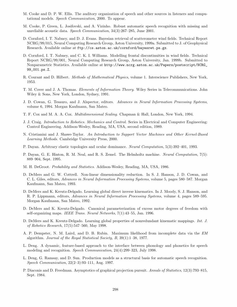
M. Cooke and D. P. W. Ellis. The auditory organization of speech and other sources in listeners and compu-tational models. Speech Communication, 2000. To appear.

M. Cooke, P. Green, L. Josifovski, and A. Vizinho. Robust automatic speech recognition with missing andunreliable acoustic data. Speech Communication, 34(3):267–285, June 2001.

D. Cornford, I. T. Nabney, and D. J. Evans. Bayesian retrieval of scatterometer wind fields. Technical ReportNCRG/99/015, Neural Computing Research Group, Aston University, 1999a. Submitted to J. of GeophysicalResearch. Available online at ftp://cs.aston.ac.uk/cornford/bayesret.ps.gz.

D. Cornford, I. T. Nabney, and C. K. I. Williams. Modelling frontal discontinuities in wind fields. TechnicalReport NCRG/99/001, Neural Computing Research Group, Aston University, Jan. 1999b. Submitted toNonparametric Statistics. Available online at http://www.ncrg.aston.ac.uk/Papers/postscript/NCRG_99_001.ps.Z.

R. Courant and D. Hilbert. Methods of Mathematical Physics, volume 1. Interscience Publishers, New York,1953.

T. M. Cover and J. A. Thomas. Elements of Information Theory. Wiley Series in Telecommunications. JohnWiley & Sons, New York, London, Sydney, 1991.

J. D. Cowan, G. Tesauro, and J. Alspector, editors. Advances in Neural Information Processing Systems,volume 6, 1994. Morgan Kaufmann, San Mateo.

T. F. Cox and M. A. A. Cox. Multidimensional Scaling. Chapman & Hall, London, New York, 1994.

J. J. Craig. Introduction to Robotics. Mechanics and Control. Series in Electrical and Computer Engineering:Control Engineering. Addison-Wesley, Reading, MA, USA, second edition, 1989.

N. Cristianini and J. Shawe-Taylor. An Introduction to Support Vector Machines and Other Kernel-BasedLearning Methods. Cambridge University Press, 2000.

P. Dayan. Arbitrary elastic topologies and ocular dominance. Neural Computation, 5(3):392–401, 1993.

P. Dayan, G. E. Hinton, R. M. Neal, and R. S. Zemel. The Helmholtz machine. Neural Computation, 7(5):889–904, Sept. 1995.

M. H. DeGroot. Probability and Statistics. Addison-Wesley, Reading, MA, USA, 1986.

D. DeMers and G. W. Cottrell. Non-linear dimensionality reduction. In S. J. Hanson, J. D. Cowan, andC. L. Giles, editors, Advances in Neural Information Processing Systems, volume 5, pages 580–587. MorganKaufmann, San Mateo, 1993.

D. DeMers and K. Kreutz-Delgado. Learning global direct inverse kinematics. In J. Moody, S. J. Hanson, andR. P. Lippmann, editors, Advances in Neural Information Processing Systems, volume 4, pages 589–595.Morgan Kaufmann, San Mateo, 1992.

D. DeMers and K. Kreutz-Delgado. Canonical parameterization of excess motor degrees of freedom withself-organizing maps. IEEE Trans. Neural Networks, 7(1):43–55, Jan. 1996.

D. DeMers and K. Kreutz-Delgado. Learning global properties of nonredundant kinematic mappings. Int. J.of Robotics Research, 17(5):547–560, May 1998.

A. P. Dempster, N. M. Laird, and D. B. Rubin. Maximum likelihood from incomplete data via the EMalgorithm. Journal of the Royal Statistical Society, B, 39(1):1–38, 1977.

L. Deng. A dynamic, feature-based approach to the interface between phonology and phonetics for speechmodeling and recognition. Speech Communication, 24(4):299–323, July 1998.

L. Deng, G. Ramsay, and D. Sun. Production models as a structural basis for automatic speech recognition.Speech Communication, 22(2–3):93–111, Aug. 1997.

P. Diaconis and D. Freedman. Asymptotics of graphical projection pursuit. Annals of Statistics, 12(3):793–815,Sept. 1984.

298

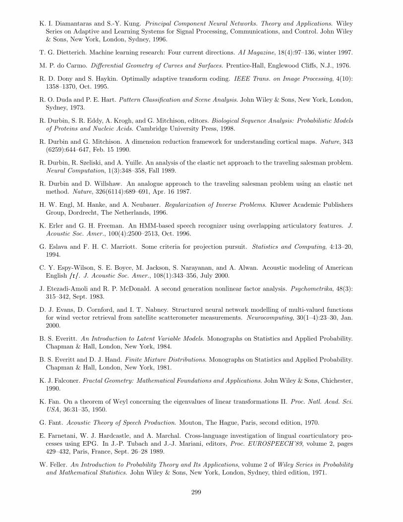
K. I. Diamantaras and S.-Y. Kung. Principal Component Neural Networks. Theory and Applications. WileySeries on Adaptive and Learning Systems for Signal Processing, Communications, and Control. John Wiley& Sons, New York, London, Sydney, 1996.

T. G. Dietterich. Machine learning research: Four current directions. AI Magazine, 18(4):97–136, winter 1997.

M. P. do Carmo. Differential Geometry of Curves and Surfaces. Prentice-Hall, Englewood Cliffs, N.J., 1976.

R. D. Dony and S. Haykin. Optimally adaptive transform coding. IEEE Trans. on Image Processing, 4(10):1358–1370, Oct. 1995.

R. O. Duda and P. E. Hart. Pattern Classification and Scene Analysis. John Wiley & Sons, New York, London,Sydney, 1973.

R. Durbin, S. R. Eddy, A. Krogh, and G. Mitchison, editors. Biological Sequence Analysis: Probabilistic Modelsof Proteins and Nucleic Acids. Cambridge University Press, 1998.

R. Durbin and G. Mitchison. A dimension reduction framework for understanding cortical maps. Nature, 343(6259):644–647, Feb. 15 1990.

R. Durbin, R. Szeliski, and A. Yuille. An analysis of the elastic net approach to the traveling salesman problem.Neural Computation, 1(3):348–358, Fall 1989.

R. Durbin and D. Willshaw. An analogue approach to the traveling salesman problem using an elastic netmethod. Nature, 326(6114):689–691, Apr. 16 1987.

H. W. Engl, M. Hanke, and A. Neubauer. Regularization of Inverse Problems. Kluwer Academic PublishersGroup, Dordrecht, The Netherlands, 1996.

K. Erler and G. H. Freeman. An HMM-based speech recognizer using overlapping articulatory features. J.Acoustic Soc. Amer., 100(4):2500–2513, Oct. 1996.

G. Eslava and F. H. C. Marriott. Some criteria for projection pursuit. Statistics and Computing, 4:13–20,1994.

C. Y. Espy-Wilson, S. E. Boyce, M. Jackson, S. Narayanan, and A. Alwan. Acoustic modeling of AmericanEnglish

�����. J. Acoustic Soc. Amer., 108(1):343–356, July 2000.

J. Etezadi-Amoli and R. P. McDonald. A second generation nonlinear factor analysis. Psychometrika, 48(3):315–342, Sept. 1983.

D. J. Evans, D. Cornford, and I. T. Nabney. Structured neural network modelling of multi-valued functionsfor wind vector retrieval from satellite scatterometer measurements. Neurocomputing, 30(1–4):23–30, Jan.2000.

B. S. Everitt. An Introduction to Latent Variable Models. Monographs on Statistics and Applied Probability.Chapman & Hall, London, New York, 1984.

B. S. Everitt and D. J. Hand. Finite Mixture Distributions. Monographs on Statistics and Applied Probability.Chapman & Hall, London, New York, 1981.

K. J. Falconer. Fractal Geometry: Mathematical Foundations and Applications. John Wiley & Sons, Chichester,1990.

K. Fan. On a theorem of Weyl concerning the eigenvalues of linear transformations II. Proc. Natl. Acad. Sci.USA, 36:31–35, 1950.

G. Fant. Acoustic Theory of Speech Production. Mouton, The Hague, Paris, second edition, 1970.

E. Farnetani, W. J. Hardcastle, and A. Marchal. Cross-language investigation of lingual coarticulatory pro-cesses using EPG. In J.-P. Tubach and J.-J. Mariani, editors, Proc. EUROSPEECH’89, volume 2, pages429–432, Paris, France, Sept. 26–28 1989.

W. Feller. An Introduction to Probability Theory and Its Applications, volume 2 of Wiley Series in Probabilityand Mathematical Statistics. John Wiley & Sons, New York, London, Sydney, third edition, 1971.

299

D. J. Field. What is the goal of sensory coding? Neural Computation, 6(4):559–601, July 1994.

J. L. Flanagan. Speech Analysis, Synthesis and Perception. Number 3 in Kommunication und Kybernetik inEinzeldarstellungen. Springer-Verlag, Berlin, second edition, 1972.

M. K. Fleming and G. W. Cottrell. Categorization of faces using unsupervised feature extraction. In Proc.Int. J. Conf. on Neural Networks (IJCNN90), volume II, pages 65–70, San Diego, CA, June 17–21 1990.

P. Foldiak. Adaptive network for optimal linear feature extraction. In Proc. Int. J. Conf. on Neural Networks(IJCNN89), volume I, pages 401–405, Washington, DC, June 18–22 1989.

D. Fotheringhame and R. Baddeley. Nonlinear principal components analysis of neuronal data. Biol. Cybern.,77(4):283–288, 1997.

I. E. Frank and J. H. Friedman. A statistical view of some chemometrics regression tools. Technometrics, 35(2):109–135 (with comments: pp. 136–148), May 1993.

J. Frankel, K. Richmond, S. King, and P. Taylor. An automatic speech recognition system using neuralnetworks and linear dynamic models to recover and model articulatory traces. In Proc. of the InternationalConference on Spoken Language Processing (ICSLP’00), Beijing, China, Oct. 16–20 2000.

J. H. Friedman. Exploratory projection pursuit. J. Amer. Stat. Assoc., 82(397):249–266, Mar. 1987.

J. H. Friedman. Multivariate adaptive regression splines. Annals of Statistics, 19(1):1–67 (with comments,pp. 67–141), Mar. 1991.

J. H. Friedman and N. I. Fisher. Bump hunting in high-dimensional data. Statistics and Computing, 9(2):123–143 (with discussion, pp. 143–162), Apr. 1999.

J. H. Friedman and W. Stuetzle. Projection pursuit regression. J. Amer. Stat. Assoc., 76(376):817–823, Dec.1981.

J. H. Friedman, W. Stuetzle, and A. Schroeder. Projection pursuit density estimation. J. Amer. Stat. Assoc.,79(387):599–608, Sept. 1984.

J. H. Friedman and J. W. Tukey. A projection pursuit algorithm for exploratory data analysis. IEEE Trans.Computers, C–23:881–889, 1974.

C. Fyfe and R. J. Baddeley. Finding compact and sparse distributed representations of visual images. Network:Computation in Neural Systems, 6(3):333–344, Aug. 1995.

J.-L. Gauvain and C.-H. Lee. Maximum a-posteriori estimation for multivariate Gaussian mixture observationsof Markov chains. IEEE Trans. Speech and Audio Process., 2:1291–1298, 1994.

A. Gelman, J. B. Carlin, H. S. Stern, and D. B. Rubin. Bayesian Data Analysis. Texts in Statistical Science.Chapman & Hall, London, New York, 1995.

C. Genest and J. V. Zidek. Combining probability distributions: A critique and an annotated bibliography.Statistical Science, 1(1):114–135 (with discussion, pp. 135–148), Feb. 1986.

Z. Ghahramani. Solving inverse problems using an EM approach to density estimation. In M. C. Mozer,P. Smolensky, D. S. Touretzky, J. L. Elman, and A. S. Weigend, editors, Proceedings of the 1993 Connec-tionist Models Summer School, pages 316–323, 1994.

Z. Ghahramani and M. J. Beal. Variational inference for Bayesian mixture of factor analysers. In Solla et al.(2000), pages 449–455.

Z. Ghahramani and G. E. Hinton. The EM algorithm for mixtures of factor analyzers. Technical ReportCRG–TR–96–1, University of Toronto, May 21 1996. Available online at ftp://ftp.cs.toronto.edu/

pub/zoubin/tr-96-1.ps.gz.

Z. Ghahramani and M. I. Jordan. Supervised learning from incomplete data via an EM approach. In Cowanet al. (1994), pages 120–127.

300

W. Gilks, S. Richardson, and D. J. Spiegelhalter, editors. Markov Chain Monte Carlo in Practice. Chapman& Hall, London, New York, 1996.

M. Girolami, A. Cichoki, and S. Amari. A common neural network model for exploratory data analysis andindependent component analysis. IEEE Trans. Neural Networks, 9(6):1495–1501, 1998.

M. Girolami and C. Fyfe. Stochastic ICA contrast maximization using Oja’s nonlinear PCA algorithm. Int.J. Neural Syst., 8(5–6):661–678, Oct./Dec. 1999.

F. Girosi, M. Jones, and T. Poggio. Regularization theory and neural networks architectures. Neural Compu-tation, 7(2):219–269, Mar. 1995.

S. J. Godsill and P. J. W. Rayner. Digital Audio Restoration: A Statistical Model-Based Approach. Springer-Verlag, Berlin, 1998a.

S. J. Godsill and P. J. W. Rayner. Robust reconstruction and analysis of autoregressive signals in impulsivenoise using the Gibbs sampler. IEEE Trans. Speech and Audio Process., 6(4):352–372, July 1998b.

B. Gold and N. Morgan. Speech and Audio Signal Processing: Processing and Perception of Speech and Music.John Wiley & Sons, New York, London, Sydney, 2000.

D. E. Goldberg. Genetic Algorithms in Search, Optimization, and Machine Learning. Addison-Wesley, 1989.

G. H. Golub and C. F. van Loan. Matrix Computations. Johns Hopkins Press, Baltimore, third edition, 1996.

G. J. Goodhill and T. J. Sejnowski. A unifying objective function for topographic mappings. Neural Compu-tation, 9(6):1291–1303, Aug. 1997.

R. A. Gopinath, B. Ramabhadran, and S. Dharanipragada. Factor analysis invariant to linear transformationsof data. In Proc. of the International Conference on Spoken Language Processing (ICSLP’98), Sydney,Australia, Nov. 30 – Dec. 4 1998.

W. P. Gouveia and J. A. Scales. Resolution of seismic waveform inversion: Bayes versus Occam. InverseProblems, 13(2):323–349, Apr. 1997.

W. P. Gouveia and J. A. Scales. Bayesian seismic waveform inversion: Parameter estimation and uncertaintyanalysis. J. of Geophysical Research, 130(B2):2759–2779, 1998.

I. S. Gradshteyn and I. M. Ryzhik. Table of Integrals, Series, and Products. Academic Press, San Diego, fifthedition, 1994. Corrected and enlarged edition, edited by Alan Jeffrey.

R. M. Gray. Vector quantization. IEEE ASSP Magazine, pages 4–29, Apr. 1984.

R. M. Gray and D. L. Neuhoff. Quantization. IEEE Trans. Inf. Theory, 44(6):2325–2383, Oct. 1998.

M. Gyllenberg, T. Koski, E. Reilink, and M. Verlaan. Non-uniqueness in probabilistic numerical identificationof bacteria. J. Appl. Prob., 31:542–548, 1994.

P. Hall. On polynomial-based projection indices for exploratory projection pursuit. Annals of Statistics, 17(2):589–605, June 1989.

W. J. Hardcastle, F. E. Gibbon, and W. Jones. Visual display of tongue-palate contact: Electropalatographyin the assessment and remediation of speech disorders. Brit. J. of Disorders of Communication, 26:41–74,1991a.

W. J. Hardcastle, F. E. Gibbon, and K. Nicolaidis. EPG data reduction methods and their implications forstudies of lingual coarticulation. J. of Phonetics, 19:251–266, 1991b.

W. J. Hardcastle and N. Hewlett, editors. Coarticulation: Theory, Data, and Techniques. Cambridge Studiesin Speech Science and Communication. Cambridge University Press, Cambridge, U.K., 1999.

W. J. Hardcastle, W. Jones, C. Knight, A. Trudgeon, and G. Calder. New developments in electropalatography:A state-of-the-art report. J. Clinical Linguistics and Phonetics, 3:1–38, 1989.

H. H. Harman. Modern Factor Analysis. University of Chicago Press, Chicago, second edition, 1967.

301

A. C. Harvey. Forecasting, Structural Time Series Models and the Kalman Filter. Cambridge University Press,1991.

T. J. Hastie and W. Stuetzle. Principal curves. J. Amer. Stat. Assoc., 84(406):502–516, June 1989.

T. J. Hastie and R. J. Tibshirani. Generalized Additive Models. Number 43 in Monographs on Statistics andApplied Probability. Chapman & Hall, London, New York, 1990.

G. T. Herman. Image Reconstruction from Projections. The Fundamentals of Computer Tomography. AcademicPress, New York, 1980.

H. Hermansky. Perceptual linear predictive (PLP) analysis of speech. J. Acoustic Soc. Amer., 87(4):1738–1752,Apr. 1990.

H. Hermansky and N. Morgan. RASTA processing of speech. IEEE Trans. Speech and Audio Process., 2(4):578–589, Oct. 1994.

J. A. Hertz, A. S. Krogh, and R. G. Palmer. Introduction to the Theory of Neural Computation. Number 1in Santa Fe Institute Studies in the Sciences of Complexity Lecture Notes. Addison-Wesley, Reading, MA,USA, 1991.

G. E. Hinton. Products of experts. In D. Wilshaw, editor, Proc. of the Ninth Int. Conf. on Artificial NeuralNetworks (ICANN99), pages 1–6, Edinburgh, UK, Sept. 7–10 1999. The Institution of Electrical Engineers.

G. E. Hinton, P. Dayan, and M. Revow. Modeling the manifolds of images of handwritten digits. IEEE Trans.Neural Networks, 8(1):65–74, Jan. 1997.

T. Holst, P. Warren, and F. Nolan. Categorising � ��� , � ��� and intermediate electropalographic patterns: Neuralnetworks and other approaches. European Journal of Disorders of Communication, 30(2):161–174, 1995.

H. Hotelling. Analysis of a complex of statistical variables into principal components. J. of EducationalPsychology, 24:417–441 and 498–520, 1933.

P. J. Huber. Robust Statistics. Wiley Series in Probability and Mathematical Statistics. John Wiley & Sons,New York, London, Sydney, 1981.

P. J. Huber. Projection pursuit. Annals of Statistics, 13(2):435–475 (with comments, pp. 475–525), June 1985.

D. Husmeier. Neural Networks for Conditional Probability Estimation. Perspectives in Neural Computing.Springer-Verlag, Berlin, 1999.

J.-N. Hwang, S.-R. Lay, M. Maechler, R. D. Martin, and J. Schimert. Regression modeling in back-propagationand projection pursuit learning. IEEE Trans. Neural Networks, 5(3):342–353, May 1994.

A. Hyvarinen. New approximations of differential entropy for independent component analysis and projectionpursuit. In Jordan et al. (1998), pages 273–279.

A. Hyvarinen. Fast and robust fixed-point algorithms for independent component analysis. IEEE Trans.Neural Networks, 10(3):626–634, Oct. 1999a.

A. Hyvarinen. Survey on independent component analysis. Neural Computing Surveys, 2:94–128, 1999b.

A. Hyvarinen, J. Karhunen, and E. Oja. Independent Component Analysis. Wiley Series on Adaptive andLearning Systems for Signal Processing, Communications, and Control. John Wiley & Sons, New York,London, Sydney, 2001.

A. Hyvarinen and E. Oja. Independent component analysis: Algorithms and applications. Neural Networks,13(4–5):411–430, June 2000.

N. Intrator and L. N. Cooper. Objective function formulation of the BCM theory of visual cortical plasticity:Statistical connections, stability conditions. Neural Networks, 5(1):3–17, 1992.

E. Isaacson and H. B. Keller. Analysis of Numerical Methods. John Wiley & Sons, New York, London, Sydney,1966.

302

M. Isard and A. Blake. CONDENSATION — conditional density propagation for visual tracking. Int. J.Computer Vision, 29(1):5–28, 1998.

J. E. Jackson. A User’s Guide to Principal Components. Wiley Series in Probability and MathematicalStatistics. John Wiley & Sons, New York, London, Sydney, 1991.

R. A. Jacobs, M. I. Jordan, S. J. Nowlan, and G. E. Hinton. Adaptive mixtures of local experts. NeuralComputation, 3(1):79–87, 1991.

M. Jamshidian and P. M. Bentler. A quasi-Newton method for minimum trace factor analysis. J. of StatisticalComputation and Simulation, 62(1–2):73–89, 1998.

N. Japkowicz, S. J. Hanson, and M. A. Gluck. Nonlinear autoassociation is not equivalent to PCA. NeuralComputation, 12(3):531–545, Mar. 2000.

E. T. Jaynes. Prior probabilities. IEEE Trans. Systems, Science, and Cybernetics, SSC-4(3):227–241, 1968.

F. V. Jensen. An Introduction to Bayesian Networks. UCL Press, London, 1996.

I. T. Jolliffe. Principal Component Analysis. Springer Series in Statistics. Springer-Verlag, Berlin, 1986.

M. C. Jones. The Projection Pursuit Algorithm for Exploratory Data Analysis. PhD thesis, University of Bath,1983.

M. C. Jones and R. Sibson. What is projection pursuit? Journal of the Royal Statistical Society, A, 150(1):1–18 (with comments, pp. 19–36), 1987.

W. Jones and W. J. Hardcastle. New developments in EPG3 software. European Journal of Disorders ofCommunication, 30(2):183–192, 1995.

M. I. Jordan. Motor learning and the degrees of freedom problem. In M. Jeannerod, editor, Attention andPerformance XIII, pages 796–836. Lawrence Erlbaum Associates, Hillsdale, New Jersey and London, 1990.

M. I. Jordan, editor. Learning in Graphical Models, Adaptive Computation and Machine Learning series, 1998.MIT Press. Proceedings of the NATO Advanced Study Institute on Learning in Graphical Models, held inErice, Italy, September 27 – October 7, 1996.

M. I. Jordan, Z. Ghahramani, T. S. Jaakkola, and L. K. Saul. An introduction to variational methods forgraphical models. Machine Learning, 37(2):183–233, Nov. 1999.

M. I. Jordan and R. A. Jacobs. Hierarchical mixtures of experts and the EM algorithm. Neural Computation,6(2):181–214, Mar. 1994.

M. I. Jordan, M. J. Kearns, and S. A. Solla, editors. Advances in Neural Information Processing Systems,volume 10, 1998. MIT Press, Cambridge, MA.

M. I. Jordan and D. E. Rumelhart. Forward models: Supervised learning with a distal teacher. CognitiveScience, 16(3):307–354, July–Sept. 1992.

K. G. Joreskog. Some contributions to maximum likelihood factor analysis. Psychometrika, 32(4):443–482,Dec. 1967.

K. G. Joreskog. A general approach to confirmatory maximum likelihood factor analysis. Psychometrika, 34(2):183–202, June 1969.

H. F. Kaiser. The varimax criterion for analytic rotation in factor analysis. Psychometrika, 23(3):187–200,Sept. 1958.

N. Kambhatla and T. K. Leen. Dimension reduction by local principal component analysis. Neural Computa-tion, 9(7):1493–1516, Oct. 1997.

G. K. Kanji. 100 Statistical Tests. Sage Publications, London, 1993.

J. N. Kapur. Maximum-Entropy Models in Science and Engineering. John Wiley & Sons, New York, London,Sydney, 1989.

303

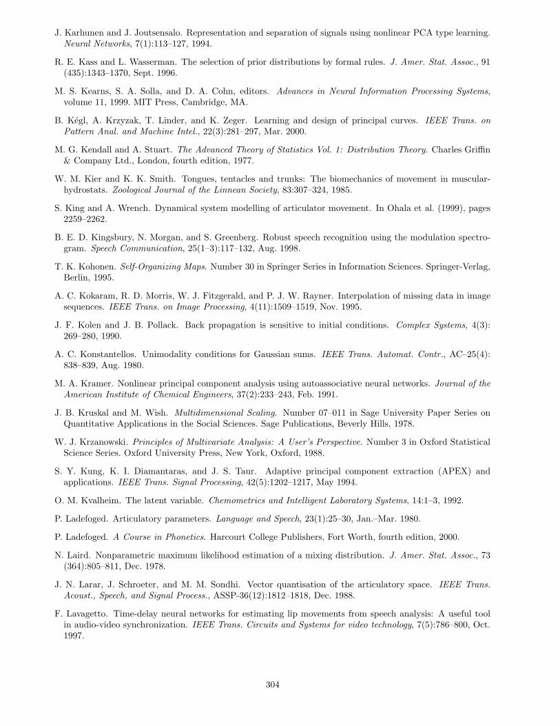
J. Karhunen and J. Joutsensalo. Representation and separation of signals using nonlinear PCA type learning.Neural Networks, 7(1):113–127, 1994.

R. E. Kass and L. Wasserman. The selection of prior distributions by formal rules. J. Amer. Stat. Assoc., 91(435):1343–1370, Sept. 1996.

M. S. Kearns, S. A. Solla, and D. A. Cohn, editors. Advances in Neural Information Processing Systems,volume 11, 1999. MIT Press, Cambridge, MA.

B. Kegl, A. Krzyzak, T. Linder, and K. Zeger. Learning and design of principal curves. IEEE Trans. onPattern Anal. and Machine Intel., 22(3):281–297, Mar. 2000.

M. G. Kendall and A. Stuart. The Advanced Theory of Statistics Vol. 1: Distribution Theory. Charles Griffin& Company Ltd., London, fourth edition, 1977.

W. M. Kier and K. K. Smith. Tongues, tentacles and trunks: The biomechanics of movement in muscular-hydrostats. Zoological Journal of the Linnean Society, 83:307–324, 1985.

S. King and A. Wrench. Dynamical system modelling of articulator movement. In Ohala et al. (1999), pages2259–2262.

B. E. D. Kingsbury, N. Morgan, and S. Greenberg. Robust speech recognition using the modulation spectro-gram. Speech Communication, 25(1–3):117–132, Aug. 1998.

T. K. Kohonen. Self-Organizing Maps. Number 30 in Springer Series in Information Sciences. Springer-Verlag,Berlin, 1995.

A. C. Kokaram, R. D. Morris, W. J. Fitzgerald, and P. J. W. Rayner. Interpolation of missing data in imagesequences. IEEE Trans. on Image Processing, 4(11):1509–1519, Nov. 1995.

J. F. Kolen and J. B. Pollack. Back propagation is sensitive to initial conditions. Complex Systems, 4(3):269–280, 1990.

A. C. Konstantellos. Unimodality conditions for Gaussian sums. IEEE Trans. Automat. Contr., AC–25(4):838–839, Aug. 1980.

M. A. Kramer. Nonlinear principal component analysis using autoassociative neural networks. Journal of theAmerican Institute of Chemical Engineers, 37(2):233–243, Feb. 1991.

J. B. Kruskal and M. Wish. Multidimensional Scaling. Number 07–011 in Sage University Paper Series onQuantitative Applications in the Social Sciences. Sage Publications, Beverly Hills, 1978.

W. J. Krzanowski. Principles of Multivariate Analysis: A User’s Perspective. Number 3 in Oxford StatisticalScience Series. Oxford University Press, New York, Oxford, 1988.

S. Y. Kung, K. I. Diamantaras, and J. S. Taur. Adaptive principal component extraction (APEX) andapplications. IEEE Trans. Signal Processing, 42(5):1202–1217, May 1994.

O. M. Kvalheim. The latent variable. Chemometrics and Intelligent Laboratory Systems, 14:1–3, 1992.

P. Ladefoged. Articulatory parameters. Language and Speech, 23(1):25–30, Jan.–Mar. 1980.

P. Ladefoged. A Course in Phonetics. Harcourt College Publishers, Fort Worth, fourth edition, 2000.

N. Laird. Nonparametric maximum likelihood estimation of a mixing distribution. J. Amer. Stat. Assoc., 73(364):805–811, Dec. 1978.

J. N. Larar, J. Schroeter, and M. M. Sondhi. Vector quantisation of the articulatory space. IEEE Trans.Acoust., Speech, and Signal Process., ASSP-36(12):1812–1818, Dec. 1988.

F. Lavagetto. Time-delay neural networks for estimating lip movements from speech analysis: A useful toolin audio-video synchronization. IEEE Trans. Circuits and Systems for video technology, 7(5):786–800, Oct.1997.

304

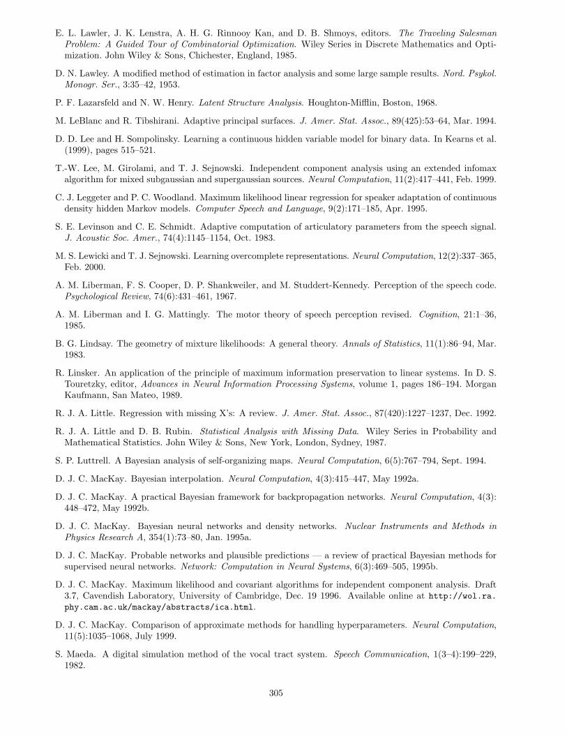
E. L. Lawler, J. K. Lenstra, A. H. G. Rinnooy Kan, and D. B. Shmoys, editors. The Traveling SalesmanProblem: A Guided Tour of Combinatorial Optimization. Wiley Series in Discrete Mathematics and Opti-mization. John Wiley & Sons, Chichester, England, 1985.

D. N. Lawley. A modified method of estimation in factor analysis and some large sample results. Nord. Psykol.Monogr. Ser., 3:35–42, 1953.

P. F. Lazarsfeld and N. W. Henry. Latent Structure Analysis. Houghton-Mifflin, Boston, 1968.

M. LeBlanc and R. Tibshirani. Adaptive principal surfaces. J. Amer. Stat. Assoc., 89(425):53–64, Mar. 1994.

D. D. Lee and H. Sompolinsky. Learning a continuous hidden variable model for binary data. In Kearns et al.(1999), pages 515–521.

T.-W. Lee, M. Girolami, and T. J. Sejnowski. Independent component analysis using an extended infomaxalgorithm for mixed subgaussian and supergaussian sources. Neural Computation, 11(2):417–441, Feb. 1999.

C. J. Leggeter and P. C. Woodland. Maximum likelihood linear regression for speaker adaptation of continuousdensity hidden Markov models. Computer Speech and Language, 9(2):171–185, Apr. 1995.

S. E. Levinson and C. E. Schmidt. Adaptive computation of articulatory parameters from the speech signal.J. Acoustic Soc. Amer., 74(4):1145–1154, Oct. 1983.

M. S. Lewicki and T. J. Sejnowski. Learning overcomplete representations. Neural Computation, 12(2):337–365,Feb. 2000.

A. M. Liberman, F. S. Cooper, D. P. Shankweiler, and M. Studdert-Kennedy. Perception of the speech code.Psychological Review, 74(6):431–461, 1967.

A. M. Liberman and I. G. Mattingly. The motor theory of speech perception revised. Cognition, 21:1–36,1985.

B. G. Lindsay. The geometry of mixture likelihoods: A general theory. Annals of Statistics, 11(1):86–94, Mar.1983.

R. Linsker. An application of the principle of maximum information preservation to linear systems. In D. S.Touretzky, editor, Advances in Neural Information Processing Systems, volume 1, pages 186–194. MorganKaufmann, San Mateo, 1989.

R. J. A. Little. Regression with missing X’s: A review. J. Amer. Stat. Assoc., 87(420):1227–1237, Dec. 1992.

R. J. A. Little and D. B. Rubin. Statistical Analysis with Missing Data. Wiley Series in Probability andMathematical Statistics. John Wiley & Sons, New York, London, Sydney, 1987.

S. P. Luttrell. A Bayesian analysis of self-organizing maps. Neural Computation, 6(5):767–794, Sept. 1994.

D. J. C. MacKay. Bayesian interpolation. Neural Computation, 4(3):415–447, May 1992a.

D. J. C. MacKay. A practical Bayesian framework for backpropagation networks. Neural Computation, 4(3):448–472, May 1992b.

D. J. C. MacKay. Bayesian neural networks and density networks. Nuclear Instruments and Methods inPhysics Research A, 354(1):73–80, Jan. 1995a.

D. J. C. MacKay. Probable networks and plausible predictions — a review of practical Bayesian methods forsupervised neural networks. Network: Computation in Neural Systems, 6(3):469–505, 1995b.

D. J. C. MacKay. Maximum likelihood and covariant algorithms for independent component analysis. Draft3.7, Cavendish Laboratory, University of Cambridge, Dec. 19 1996. Available online at http://wol.ra.

phy.cam.ac.uk/mackay/abstracts/ica.html.

D. J. C. MacKay. Comparison of approximate methods for handling hyperparameters. Neural Computation,11(5):1035–1068, July 1999.

S. Maeda. A digital simulation method of the vocal tract system. Speech Communication, 1(3–4):199–229,1982.

305

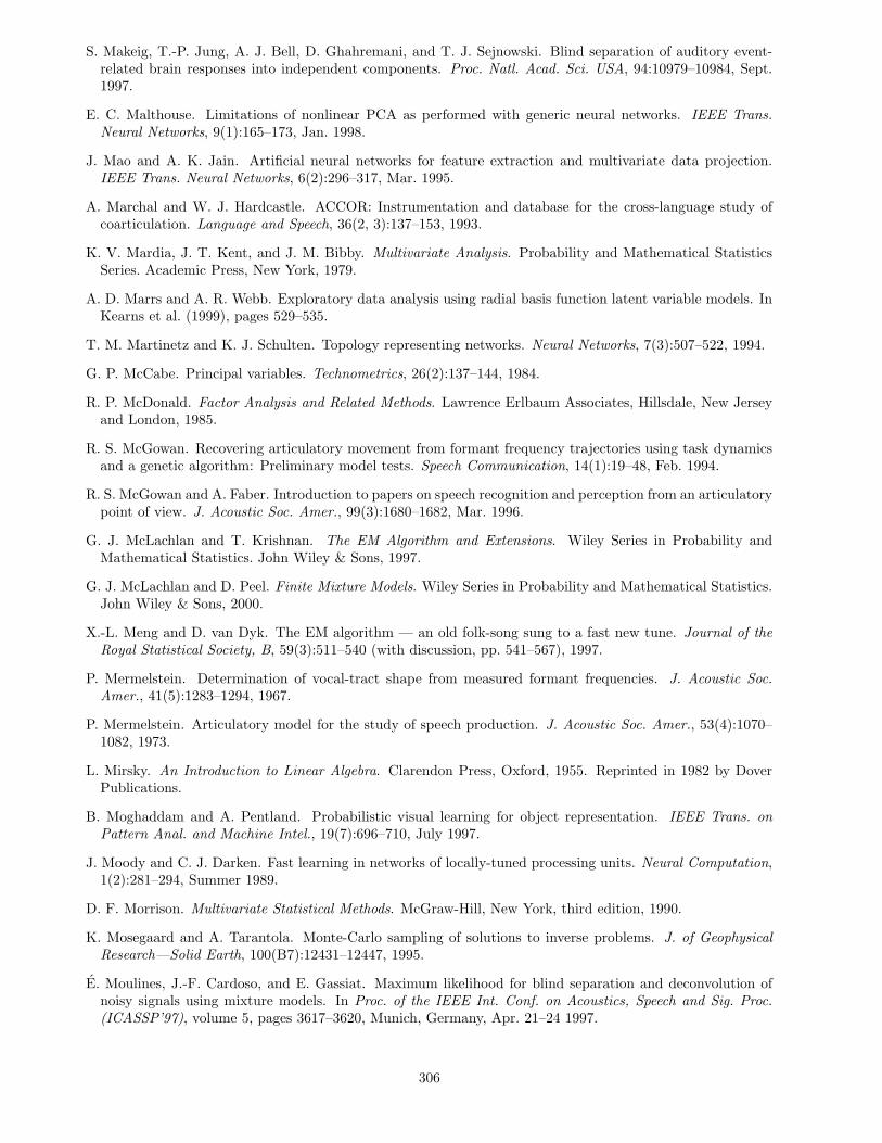
S. Makeig, T.-P. Jung, A. J. Bell, D. Ghahremani, and T. J. Sejnowski. Blind separation of auditory event-related brain responses into independent components. Proc. Natl. Acad. Sci. USA, 94:10979–10984, Sept.1997.

E. C. Malthouse. Limitations of nonlinear PCA as performed with generic neural networks. IEEE Trans.Neural Networks, 9(1):165–173, Jan. 1998.

J. Mao and A. K. Jain. Artificial neural networks for feature extraction and multivariate data projection.IEEE Trans. Neural Networks, 6(2):296–317, Mar. 1995.

A. Marchal and W. J. Hardcastle. ACCOR: Instrumentation and database for the cross-language study ofcoarticulation. Language and Speech, 36(2, 3):137–153, 1993.

K. V. Mardia, J. T. Kent, and J. M. Bibby. Multivariate Analysis. Probability and Mathematical StatisticsSeries. Academic Press, New York, 1979.

A. D. Marrs and A. R. Webb. Exploratory data analysis using radial basis function latent variable models. InKearns et al. (1999), pages 529–535.

T. M. Martinetz and K. J. Schulten. Topology representing networks. Neural Networks, 7(3):507–522, 1994.

G. P. McCabe. Principal variables. Technometrics, 26(2):137–144, 1984.

R. P. McDonald. Factor Analysis and Related Methods. Lawrence Erlbaum Associates, Hillsdale, New Jerseyand London, 1985.

R. S. McGowan. Recovering articulatory movement from formant frequency trajectories using task dynamicsand a genetic algorithm: Preliminary model tests. Speech Communication, 14(1):19–48, Feb. 1994.

R. S. McGowan and A. Faber. Introduction to papers on speech recognition and perception from an articulatorypoint of view. J. Acoustic Soc. Amer., 99(3):1680–1682, Mar. 1996.

G. J. McLachlan and T. Krishnan. The EM Algorithm and Extensions. Wiley Series in Probability andMathematical Statistics. John Wiley & Sons, 1997.

G. J. McLachlan and D. Peel. Finite Mixture Models. Wiley Series in Probability and Mathematical Statistics.John Wiley & Sons, 2000.

X.-L. Meng and D. van Dyk. The EM algorithm — an old folk-song sung to a fast new tune. Journal of theRoyal Statistical Society, B, 59(3):511–540 (with discussion, pp. 541–567), 1997.

P. Mermelstein. Determination of vocal-tract shape from measured formant frequencies. J. Acoustic Soc.Amer., 41(5):1283–1294, 1967.

P. Mermelstein. Articulatory model for the study of speech production. J. Acoustic Soc. Amer., 53(4):1070–1082, 1973.

L. Mirsky. An Introduction to Linear Algebra. Clarendon Press, Oxford, 1955. Reprinted in 1982 by DoverPublications.

B. Moghaddam and A. Pentland. Probabilistic visual learning for object representation. IEEE Trans. onPattern Anal. and Machine Intel., 19(7):696–710, July 1997.

J. Moody and C. J. Darken. Fast learning in networks of locally-tuned processing units. Neural Computation,1(2):281–294, Summer 1989.

D. F. Morrison. Multivariate Statistical Methods. McGraw-Hill, New York, third edition, 1990.

K. Mosegaard and A. Tarantola. Monte-Carlo sampling of solutions to inverse problems. J. of GeophysicalResearch—Solid Earth, 100(B7):12431–12447, 1995.

E. Moulines, J.-F. Cardoso, and E. Gassiat. Maximum likelihood for blind separation and deconvolution ofnoisy signals using mixture models. In Proc. of the IEEE Int. Conf. on Acoustics, Speech and Sig. Proc.(ICASSP’97), volume 5, pages 3617–3620, Munich, Germany, Apr. 21–24 1997.

306

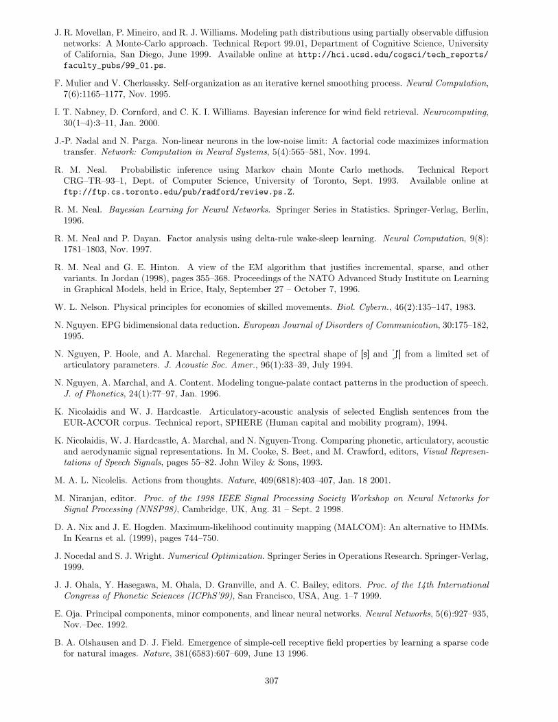
J. R. Movellan, P. Mineiro, and R. J. Williams. Modeling path distributions using partially observable diffusionnetworks: A Monte-Carlo approach. Technical Report 99.01, Department of Cognitive Science, Universityof California, San Diego, June 1999. Available online at http://hci.ucsd.edu/cogsci/tech_reports/

faculty_pubs/99_01.ps.

F. Mulier and V. Cherkassky. Self-organization as an iterative kernel smoothing process. Neural Computation,7(6):1165–1177, Nov. 1995.

I. T. Nabney, D. Cornford, and C. K. I. Williams. Bayesian inference for wind field retrieval. Neurocomputing,30(1–4):3–11, Jan. 2000.

J.-P. Nadal and N. Parga. Non-linear neurons in the low-noise limit: A factorial code maximizes informationtransfer. Network: Computation in Neural Systems, 5(4):565–581, Nov. 1994.

R. M. Neal. Probabilistic inference using Markov chain Monte Carlo methods. Technical ReportCRG–TR–93–1, Dept. of Computer Science, University of Toronto, Sept. 1993. Available online atftp://ftp.cs.toronto.edu/pub/radford/review.ps.Z.

R. M. Neal. Bayesian Learning for Neural Networks. Springer Series in Statistics. Springer-Verlag, Berlin,1996.

R. M. Neal and P. Dayan. Factor analysis using delta-rule wake-sleep learning. Neural Computation, 9(8):1781–1803, Nov. 1997.

R. M. Neal and G. E. Hinton. A view of the EM algorithm that justifies incremental, sparse, and othervariants. In Jordan (1998), pages 355–368. Proceedings of the NATO Advanced Study Institute on Learningin Graphical Models, held in Erice, Italy, September 27 – October 7, 1996.

W. L. Nelson. Physical principles for economies of skilled movements. Biol. Cybern., 46(2):135–147, 1983.

N. Nguyen. EPG bidimensional data reduction. European Journal of Disorders of Communication, 30:175–182,1995.

N. Nguyen, P. Hoole, and A. Marchal. Regenerating the spectral shape of � ��� and � ��� from a limited set ofarticulatory parameters. J. Acoustic Soc. Amer., 96(1):33–39, July 1994.

N. Nguyen, A. Marchal, and A. Content. Modeling tongue-palate contact patterns in the production of speech.J. of Phonetics, 24(1):77–97, Jan. 1996.

K. Nicolaidis and W. J. Hardcastle. Articulatory-acoustic analysis of selected English sentences from theEUR-ACCOR corpus. Technical report, SPHERE (Human capital and mobility program), 1994.

K. Nicolaidis, W. J. Hardcastle, A. Marchal, and N. Nguyen-Trong. Comparing phonetic, articulatory, acousticand aerodynamic signal representations. In M. Cooke, S. Beet, and M. Crawford, editors, Visual Represen-tations of Speech Signals, pages 55–82. John Wiley & Sons, 1993.

M. A. L. Nicolelis. Actions from thoughts. Nature, 409(6818):403–407, Jan. 18 2001.

M. Niranjan, editor. Proc. of the 1998 IEEE Signal Processing Society Workshop on Neural Networks forSignal Processing (NNSP98), Cambridge, UK, Aug. 31 – Sept. 2 1998.

D. A. Nix and J. E. Hogden. Maximum-likelihood continuity mapping (MALCOM): An alternative to HMMs.In Kearns et al. (1999), pages 744–750.

J. Nocedal and S. J. Wright. Numerical Optimization. Springer Series in Operations Research. Springer-Verlag,1999.

J. J. Ohala, Y. Hasegawa, M. Ohala, D. Granville, and A. C. Bailey, editors. Proc. of the 14th InternationalCongress of Phonetic Sciences (ICPhS’99), San Francisco, USA, Aug. 1–7 1999.

E. Oja. Principal components, minor components, and linear neural networks. Neural Networks, 5(6):927–935,Nov.–Dec. 1992.

B. A. Olshausen and D. J. Field. Emergence of simple-cell receptive field properties by learning a sparse codefor natural images. Nature, 381(6583):607–609, June 13 1996.

307

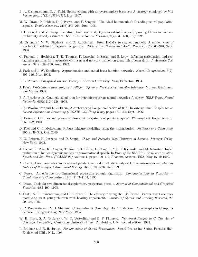
B. A. Olshausen and D. J. Field. Sparse coding with an overcomplete basis set: A strategy employed by V1?Vision Res., 37(23):3311–3325, Dec. 1997.

M. W. Oram, P. Foldiak, D. I. Perret, and F. Sengpiel. The ‘ideal homunculus’: Decoding neural populationsignals. Trends Neurosci., 21(6):259–265, June 1998.

D. Ormoneit and V. Tresp. Penalized likelihood and Bayesian estimation for improving Gaussian mixtureprobability density estimates. IEEE Trans. Neural Networks, 9(4):639–650, July 1998.

M. Ostendorf, V. V. Digalakis, and O. A. Kimball. From HMM’s to segment models: A unified view ofstochastic modeling for speech recognition. IEEE Trans. Speech and Audio Process., 4(5):360–378, Sept.1996.

G. Papcun, J. Hochberg, T. R. Thomas, F. Laroche, J. Zacks, and S. Levy. Inferring articulation and rec-ognizing gestures from acoustics with a neural network trained on x-ray microbeam data. J. Acoustic Soc.Amer., 92(2):688–700, Aug. 1992.

J. Park and I. W. Sandberg. Approximation and radial-basis-function networks. Neural Computation, 5(2):305–316, Mar. 1993.

R. L. Parker. Geophysical Inverse Theory. Princeton University Press, Princeton, 1994.

J. Pearl. Probabilistic Reasoning in Intelligent Systems: Networks of Plausible Inference. Morgan Kaufmann,San Mateo, 1988.

B. A. Pearlmutter. Gradient calculation for dynamic recurrent neural networks: A survey. IEEE Trans. NeuralNetworks, 6(5):1212–1228, 1995.

B. A. Pearlmutter and L. C. Parra. A context-sensitive generalization of ICA. In International Conference onNeural Information Processing (ICONIP–96), Hong Kong, pages 151–157, Sept. 1996.

K. Pearson. On lines and planes of closest fit to systems of points in space. Philosophical Magazine, 2(6):559–572, 1901.

D. Peel and G. J. McLachlan. Robust mixture modelling using the t distribution. Statistics and Computing,10(4):339–348, Oct. 2000.

H.-O. Peitgen, H. Jurgens, and D. Saupe. Chaos and Fractals: New Frontiers of Science. Springer-Verlag,New York, 1992.

J. Picone, S. Pike, R. Reagan, T. Kamm, J. Bridle, L. Deng, J. Ma, H. Richards, and M. Schuster. Initialevaluation of hidden dynamic models on conversational speech. In Proc. of the IEEE Int. Conf. on Acoustics,Speech and Sig. Proc. (ICASSP’99), volume 1, pages 109–112, Phoenix, Arizona, USA, May 15–19 1999.

A. Pisani. A nonparametric and scale-independent method for cluster-analysis. 1. The univariate case. MonthlyNotices of the Royal Astronomical Society, 265(3):706–726, Dec. 1993.

C. Posse. An effective two-dimensional projection pursuit algorithm. Communications in Statistics —Simulation and Computation, 19(4):1143–1164, 1990.

C. Posse. Tools for two-dimensional exploratory projection pursuit. Journal of Computational and GraphicalStatistics, 4:83–100, 1995.

S. Pratt, A. T. Heintzelman, and D. S. Ensrud. The efficacy of using the IBM Speech Viewer vowel accuracymodule to treat young children with hearing impairment. Journal of Speech and Hearing Research, 29:99–105, 1993.

F. P. Preparata and M. I. Shamos. Computational Geometry: An Introduction. Monographs in ComputerScience. Springer-Verlag, New York, 1985.

W. H. Press, S. A. Teukolsky, W. T. Vetterling, and B. P. Flannery. Numerical Recipes in C: The Art ofScientific Computing. Cambridge University Press, Cambridge, U.K., second edition, 1992.

L. Rabiner and B.-H. Juang. Fundamentals of Speech Recognition. Signal Processing Series. Prentice-Hall,Englewood Cliffs, N.J., 1993.

308

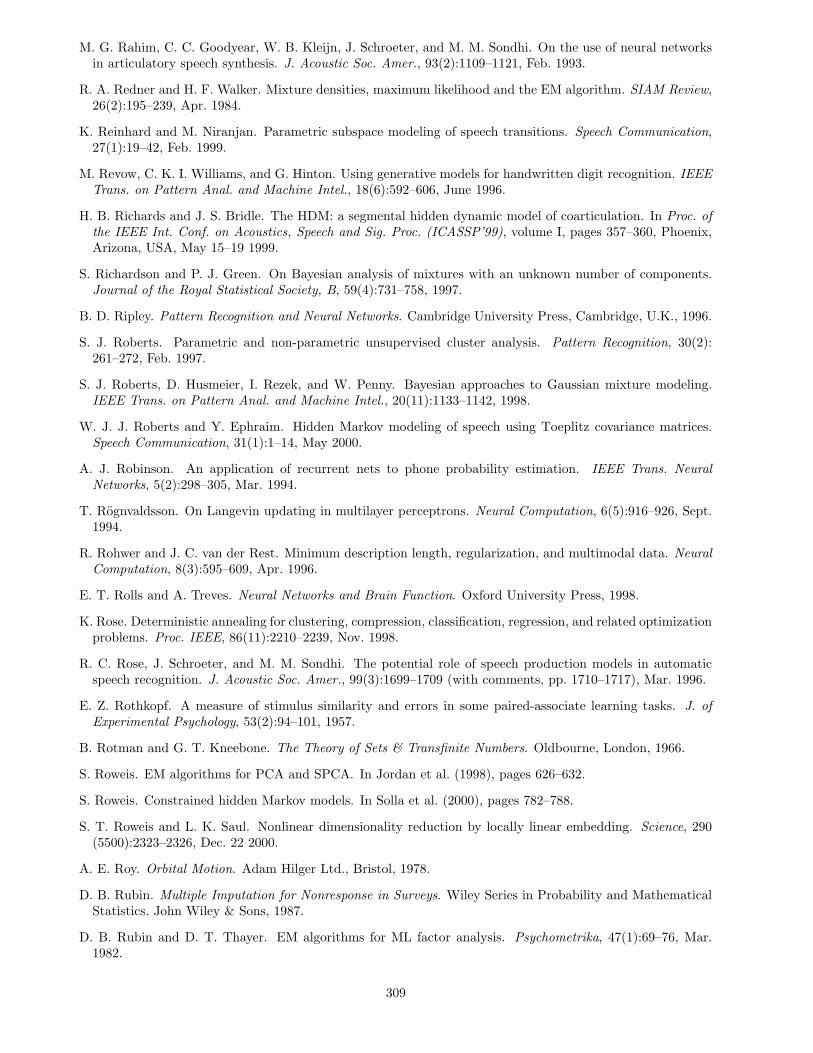
M. G. Rahim, C. C. Goodyear, W. B. Kleijn, J. Schroeter, and M. M. Sondhi. On the use of neural networksin articulatory speech synthesis. J. Acoustic Soc. Amer., 93(2):1109–1121, Feb. 1993.

R. A. Redner and H. F. Walker. Mixture densities, maximum likelihood and the EM algorithm. SIAM Review,26(2):195–239, Apr. 1984.

K. Reinhard and M. Niranjan. Parametric subspace modeling of speech transitions. Speech Communication,27(1):19–42, Feb. 1999.

M. Revow, C. K. I. Williams, and G. Hinton. Using generative models for handwritten digit recognition. IEEETrans. on Pattern Anal. and Machine Intel., 18(6):592–606, June 1996.

H. B. Richards and J. S. Bridle. The HDM: a segmental hidden dynamic model of coarticulation. In Proc. ofthe IEEE Int. Conf. on Acoustics, Speech and Sig. Proc. (ICASSP’99), volume I, pages 357–360, Phoenix,Arizona, USA, May 15–19 1999.

S. Richardson and P. J. Green. On Bayesian analysis of mixtures with an unknown number of components.Journal of the Royal Statistical Society, B, 59(4):731–758, 1997.

B. D. Ripley. Pattern Recognition and Neural Networks. Cambridge University Press, Cambridge, U.K., 1996.

S. J. Roberts. Parametric and non-parametric unsupervised cluster analysis. Pattern Recognition, 30(2):261–272, Feb. 1997.

S. J. Roberts, D. Husmeier, I. Rezek, and W. Penny. Bayesian approaches to Gaussian mixture modeling.IEEE Trans. on Pattern Anal. and Machine Intel., 20(11):1133–1142, 1998.

W. J. J. Roberts and Y. Ephraim. Hidden Markov modeling of speech using Toeplitz covariance matrices.Speech Communication, 31(1):1–14, May 2000.

A. J. Robinson. An application of recurrent nets to phone probability estimation. IEEE Trans. NeuralNetworks, 5(2):298–305, Mar. 1994.

T. Rognvaldsson. On Langevin updating in multilayer perceptrons. Neural Computation, 6(5):916–926, Sept.1994.

R. Rohwer and J. C. van der Rest. Minimum description length, regularization, and multimodal data. NeuralComputation, 8(3):595–609, Apr. 1996.

E. T. Rolls and A. Treves. Neural Networks and Brain Function. Oxford University Press, 1998.

K. Rose. Deterministic annealing for clustering, compression, classification, regression, and related optimizationproblems. Proc. IEEE, 86(11):2210–2239, Nov. 1998.

R. C. Rose, J. Schroeter, and M. M. Sondhi. The potential role of speech production models in automaticspeech recognition. J. Acoustic Soc. Amer., 99(3):1699–1709 (with comments, pp. 1710–1717), Mar. 1996.

E. Z. Rothkopf. A measure of stimulus similarity and errors in some paired-associate learning tasks. J. ofExperimental Psychology, 53(2):94–101, 1957.

B. Rotman and G. T. Kneebone. The Theory of Sets & Transfinite Numbers. Oldbourne, London, 1966.

S. Roweis. EM algorithms for PCA and SPCA. In Jordan et al. (1998), pages 626–632.

S. Roweis. Constrained hidden Markov models. In Solla et al. (2000), pages 782–788.

S. T. Roweis and L. K. Saul. Nonlinear dimensionality reduction by locally linear embedding. Science, 290(5500):2323–2326, Dec. 22 2000.

A. E. Roy. Orbital Motion. Adam Hilger Ltd., Bristol, 1978.

D. B. Rubin. Multiple Imputation for Nonresponse in Surveys. Wiley Series in Probability and MathematicalStatistics. John Wiley & Sons, 1987.

D. B. Rubin and D. T. Thayer. EM algorithms for ML factor analysis. Psychometrika, 47(1):69–76, Mar.1982.

309

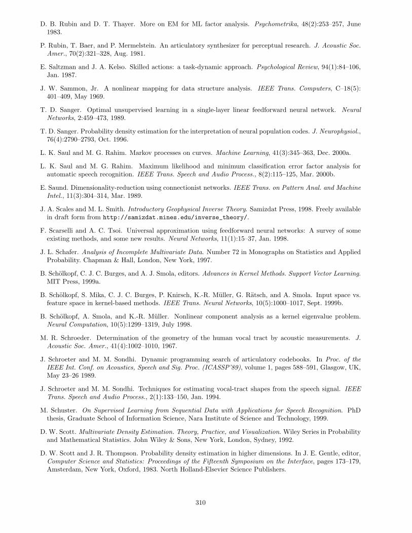
D. B. Rubin and D. T. Thayer. More on EM for ML factor analysis. Psychometrika, 48(2):253–257, June1983.

P. Rubin, T. Baer, and P. Mermelstein. An articulatory synthesizer for perceptual research. J. Acoustic Soc.Amer., 70(2):321–328, Aug. 1981.

E. Saltzman and J. A. Kelso. Skilled actions: a task-dynamic approach. Psychological Review, 94(1):84–106,Jan. 1987.

J. W. Sammon, Jr. A nonlinear mapping for data structure analysis. IEEE Trans. Computers, C–18(5):401–409, May 1969.

T. D. Sanger. Optimal unsupervised learning in a single-layer linear feedforward neural network. NeuralNetworks, 2:459–473, 1989.

T. D. Sanger. Probability density estimation for the interpretation of neural population codes. J. Neurophysiol.,76(4):2790–2793, Oct. 1996.

L. K. Saul and M. G. Rahim. Markov processes on curves. Machine Learning, 41(3):345–363, Dec. 2000a.

L. K. Saul and M. G. Rahim. Maximum likelihood and minimum classification error factor analysis forautomatic speech recognition. IEEE Trans. Speech and Audio Process., 8(2):115–125, Mar. 2000b.

E. Saund. Dimensionality-reduction using connectionist networks. IEEE Trans. on Pattern Anal. and MachineIntel., 11(3):304–314, Mar. 1989.

J. A. Scales and M. L. Smith. Introductory Geophysical Inverse Theory. Samizdat Press, 1998. Freely availablein draft form from http://samizdat.mines.edu/inverse_theory/.

F. Scarselli and A. C. Tsoi. Universal approximation using feedforward neural networks: A survey of someexisting methods, and some new results. Neural Networks, 11(1):15–37, Jan. 1998.

J. L. Schafer. Analysis of Incomplete Multivariate Data. Number 72 in Monographs on Statistics and AppliedProbability. Chapman & Hall, London, New York, 1997.

B. Scholkopf, C. J. C. Burges, and A. J. Smola, editors. Advances in Kernel Methods. Support Vector Learning.MIT Press, 1999a.

B. Scholkopf, S. Mika, C. J. C. Burges, P. Knirsch, K.-R. Muller, G. Ratsch, and A. Smola. Input space vs.feature space in kernel-based methods. IEEE Trans. Neural Networks, 10(5):1000–1017, Sept. 1999b.

B. Scholkopf, A. Smola, and K.-R. Muller. Nonlinear component analysis as a kernel eigenvalue problem.Neural Computation, 10(5):1299–1319, July 1998.

M. R. Schroeder. Determination of the geometry of the human vocal tract by acoustic measurements. J.Acoustic Soc. Amer., 41(4):1002–1010, 1967.

J. Schroeter and M. M. Sondhi. Dynamic programming search of articulatory codebooks. In Proc. of theIEEE Int. Conf. on Acoustics, Speech and Sig. Proc. (ICASSP’89), volume 1, pages 588–591, Glasgow, UK,May 23–26 1989.

J. Schroeter and M. M. Sondhi. Techniques for estimating vocal-tract shapes from the speech signal. IEEETrans. Speech and Audio Process., 2(1):133–150, Jan. 1994.

M. Schuster. On Supervised Learning from Sequential Data with Applications for Speech Recognition. PhDthesis, Graduate School of Information Science, Nara Institute of Science and Technology, 1999.

D. W. Scott. Multivariate Density Estimation. Theory, Practice, and Visualization. Wiley Series in Probabilityand Mathematical Statistics. John Wiley & Sons, New York, London, Sydney, 1992.

D. W. Scott and J. R. Thompson. Probability density estimation in higher dimensions. In J. E. Gentle, editor,Computer Science and Statistics: Proceedings of the Fifteenth Symposium on the Interface, pages 173–179,Amsterdam, New York, Oxford, 1983. North Holland-Elsevier Science Publishers.

310

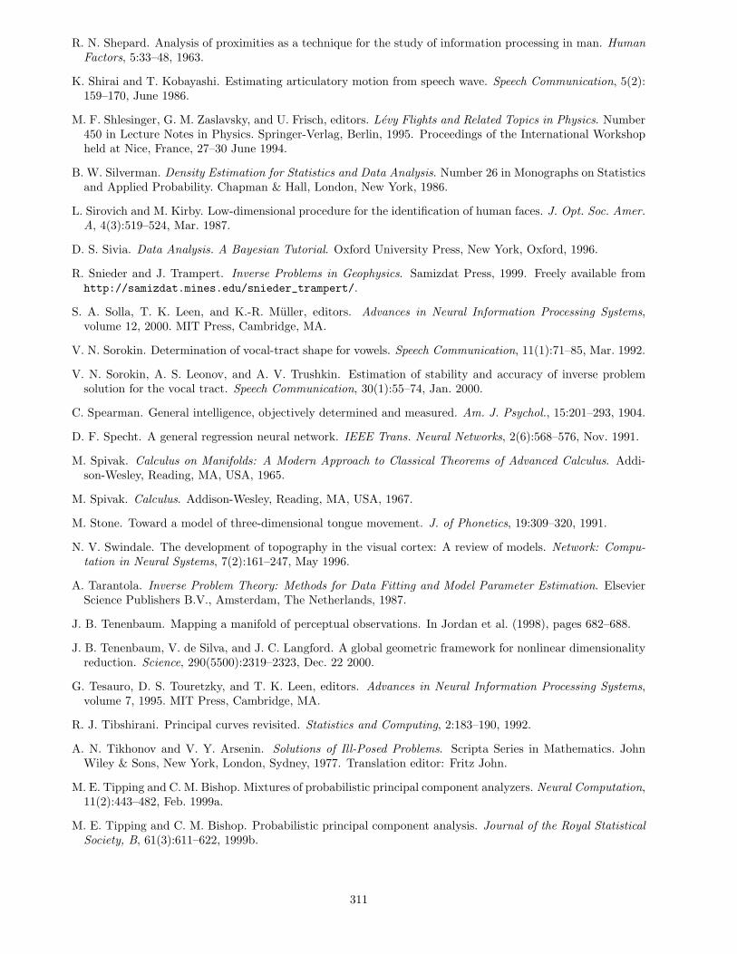
R. N. Shepard. Analysis of proximities as a technique for the study of information processing in man. HumanFactors, 5:33–48, 1963.

K. Shirai and T. Kobayashi. Estimating articulatory motion from speech wave. Speech Communication, 5(2):159–170, June 1986.

M. F. Shlesinger, G. M. Zaslavsky, and U. Frisch, editors. Levy Flights and Related Topics in Physics. Number450 in Lecture Notes in Physics. Springer-Verlag, Berlin, 1995. Proceedings of the International Workshopheld at Nice, France, 27–30 June 1994.

B. W. Silverman. Density Estimation for Statistics and Data Analysis. Number 26 in Monographs on Statisticsand Applied Probability. Chapman & Hall, London, New York, 1986.

L. Sirovich and M. Kirby. Low-dimensional procedure for the identification of human faces. J. Opt. Soc. Amer.A, 4(3):519–524, Mar. 1987.

D. S. Sivia. Data Analysis. A Bayesian Tutorial. Oxford University Press, New York, Oxford, 1996.

R. Snieder and J. Trampert. Inverse Problems in Geophysics. Samizdat Press, 1999. Freely available fromhttp://samizdat.mines.edu/snieder_trampert/.

S. A. Solla, T. K. Leen, and K.-R. Muller, editors. Advances in Neural Information Processing Systems,volume 12, 2000. MIT Press, Cambridge, MA.

V. N. Sorokin. Determination of vocal-tract shape for vowels. Speech Communication, 11(1):71–85, Mar. 1992.

V. N. Sorokin, A. S. Leonov, and A. V. Trushkin. Estimation of stability and accuracy of inverse problemsolution for the vocal tract. Speech Communication, 30(1):55–74, Jan. 2000.

C. Spearman. General intelligence, objectively determined and measured. Am. J. Psychol., 15:201–293, 1904.

D. F. Specht. A general regression neural network. IEEE Trans. Neural Networks, 2(6):568–576, Nov. 1991.

M. Spivak. Calculus on Manifolds: A Modern Approach to Classical Theorems of Advanced Calculus. Addi-son-Wesley, Reading, MA, USA, 1965.

M. Spivak. Calculus. Addison-Wesley, Reading, MA, USA, 1967.

M. Stone. Toward a model of three-dimensional tongue movement. J. of Phonetics, 19:309–320, 1991.

N. V. Swindale. The development of topography in the visual cortex: A review of models. Network: Compu-tation in Neural Systems, 7(2):161–247, May 1996.

A. Tarantola. Inverse Problem Theory: Methods for Data Fitting and Model Parameter Estimation. ElsevierScience Publishers B.V., Amsterdam, The Netherlands, 1987.

J. B. Tenenbaum. Mapping a manifold of perceptual observations. In Jordan et al. (1998), pages 682–688.

J. B. Tenenbaum, V. de Silva, and J. C. Langford. A global geometric framework for nonlinear dimensionalityreduction. Science, 290(5500):2319–2323, Dec. 22 2000.

G. Tesauro, D. S. Touretzky, and T. K. Leen, editors. Advances in Neural Information Processing Systems,volume 7, 1995. MIT Press, Cambridge, MA.

R. J. Tibshirani. Principal curves revisited. Statistics and Computing, 2:183–190, 1992.

A. N. Tikhonov and V. Y. Arsenin. Solutions of Ill-Posed Problems. Scripta Series in Mathematics. JohnWiley & Sons, New York, London, Sydney, 1977. Translation editor: Fritz John.

M. E. Tipping and C. M. Bishop. Mixtures of probabilistic principal component analyzers. Neural Computation,11(2):443–482, Feb. 1999a.

M. E. Tipping and C. M. Bishop. Probabilistic principal component analysis. Journal of the Royal StatisticalSociety, B, 61(3):611–622, 1999b.

311

D. M. Titterington, A. F. M. Smith, and U. E. Makov. Statistical Analysis of Finite Mixture Distributions.Wiley Series in Probability and Mathematical Statistics. John Wiley & Sons, New York, London, Sydney,1985.

L. Tong, R.-W. Liu, V. C. Soon, and Y.-F. Huang. The indeterminacy and identifiability of blind identification.IEEE Trans. Circuits and Systems, 38(5):499–509, May 1991.

V. Tresp, R. Neuneier, and S. Ahmad. Efficient methods for dealing with missing data in supervised learning.In Tesauro et al. (1995), pages 689–696.

A. Treves, S. Panzeri, E. T. Rolls, M. Booth, and E. A. Wakeman. Firing rate distributions and efficiency ofinformation transmission of inferior temporal cortex neurons to natural visual stimuli. Neural Computation,11(3):601–632, Mar. 1999.

A. Treves and E. T. Rolls. What determines the capacity of autoassociative memories in the brain? Network:Computation in Neural Systems, 2(4):371–397, Nov. 1991.

A. C. Tsoi. Recurrent neural network architectures — an overview. In C. L. Giles and M. Gori, editors,Adaptive Processing of Temporal Information, volume 1387 of Lecture Notes in Artificial Intelligence, pages1–26. Springer-Verlag, New York, 1998.

UCLA. Artificial EPG palate image. The UCLA Phonetics Lab. Available online at http://www.humnet.

ucla.edu/humnet/linguistics/faciliti/facilities/physiology/EGP_picture.JPG, Feb. 1, 2000.

N. Ueda, R. Nakano, Z. Ghahramani, and G. E. Hinton. SMEM algorithm for mixture models. NeuralComputation, 12(9):2109–2128, Sept. 2000.

A. Utsugi. Hyperparameter selection for self-organizing maps. Neural Computation, 9(3):623–635, Apr. 1997a.

A. Utsugi. Topology selection for self-organizing maps. Network: Computation in Neural Systems, 7(4):727–740, 1997b.

A. Utsugi. Bayesian sampling and ensemble learning in generative topographic mapping. Neural ProcessingLetters, 12(3):277–290, Dec. 2000.

A. Utsugi and T. Kumagai. Bayesian analysis of mixtures of factor analyzers. Neural Computation, 13(5):993–1002, May 2001.

V. N. Vapnik and S. Mukherjee. Support vector method for multivariate density estimation. In Solla et al.(2000), pages 659–665.

S. V. Vaseghi. Advanced Signal Processing and Digital Noise Reduction. John Wiley & Sons, New York,London, Sydney, second edition, 2000.

S. V. Vaseghi and P. J. W. Rayner. Detection and suppression of impulsive noise in speech-communicationsystems. IEE Proc. I (Communications, Speech and Vision), 137(1):38–46, Feb. 1990.

T. Villmann, R. Der, M. Hermann, and T. M. Martinetz. Topology preservation in self-organizing featuremaps: Exact definition and measurement. IEEE Trans. Neural Networks, 8(2):256–266, Mar. 1997.

W. E. Vinje and J. L. Gallant. Sparse coding and decorrelation in primary visual cortex during natural vision.Science, 287(5456):1273–1276, Feb. 18 2000.

H. M. Wagner. Principles of Operations Research with Applications to Managerial Decisions. Prentice-Hall,Englewood Cliffs, N.J., second edition, 1975.

A. Webb. Statistical Pattern Recognition. Edward Arnold, 1999.

A. R. Webb. Multidimensional scaling by iterative majorization using radial basis functions. Pattern Recog-nition, 28(5):753–759, May 1995.

E. J. Wegman. Hyperdimensional data analysis using parallel coordinates. J. Amer. Stat. Assoc., 85(411):664–675, Sept. 1990.

312

J. R. Westbury. X-Ray Microbeam Speech Production Database User’s Handbook Version 1.0. Waisman Centeron Mental Retardation & Human Development, University of Wisconsin, Madison, WI, June 1994. Withthe assistance of Greg Turner & Jim Dembowski.

J. R. Westbury, M. Hashi, and M. J. Lindstrom. Differences among speakers in lingual articulation for AmericanEnglish

�����. Speech Communication, 26(3):203–226, Nov. 1998.

J. Weston, A. Gammerman, M. O. Stitson, V. Vapnik, V. Vovk, and C. Watkins. Support vector densityestimation. In Scholkopf et al. (1999a), chapter 18, pages 293–306.

J. Whittaker. Graphical Models in Applied Multivariate Statistics. Wiley Series in Probability and Mathemat-ical Statistics. John Wiley & Sons, New York, London, Sydney, 1990.

P. Whittle. On principal components and least square methods of factor analysis. Skand. Aktur. Tidskr., 36:223–239, 1952.

J. Wiles, P. Bakker, A. Lynton, M. Norris, S. Parkinson, M. Staples, and A. Whiteside. Using bottlenecksin feedforward networks as a dimension reduction technique: An application to optimization tasks. NeuralComputation, 8(6):1179–1183, Aug. 1996.

J. H. Wilkinson. The Algebraic Eigenvalue Problem. Oxford University Press, New York, Oxford, 1965.

P. M. Williams. Using neural networks to model conditional multivariate densities. Neural Computation, 8(4):843–854, May 1996.

B. Willmore, P. A. Watters, and D. J. Tolhurst. A comparison of natural-image-based models of simple-cellcoding. Perception, 29(9):1017–1040, Sept. 2000.

R. Wilson and M. Spann. A new approach to clustering. Pattern Recognition, 23(12):1413–1425, 1990.

J. H. Wolfe. Pattern clustering by multivariate mixture analysis. Multivariate Behavioral Research, 5:329–350,July 1970.

D. M. Wolpert and Z. Ghahramani. Computational principles of movement neuroscience. Nat. Neurosci., 3(Supp.):1212–1217, Nov. 2000.

D. M. Wolpert and M. Kawato. Multiple paired forward and inverse models for motor control. Neural Networks,11(7–8):1317–1329, Oct. 1998.

A. A. Wrench. A multi-channel/multi-speaker articulatory database for continuous speech recognition research.In Phonus, volume 5, Saarbrucken, 2000. Institute of Phonetics, University of Saarland.

F. Xie and D. van Compernolle. Speech enhancement by spectral magnitude estimation —a unifying approach.Speech Communication, 19(2):89–104, Aug. 1996.

L. Xu, C. C. Cheung, and S. Amari. Learned parametric mixture based ICA algorithm. Neurocomputing, 22(1–3):69–80, Nov. 1998.

E. Yamamoto, S. Nakamura, and K. Shikano. Lip movement synthesis from speech based on hidden Markovmodels. Speech Communication, 26(1–2):105–115, 1998.

H. H. Yang and S. Amari. Adaptive on-line learning algorithms for blind separation — maximum entropy andminimum mutual information. Neural Computation, 9(7):1457–1482, Oct. 1997.

H. Yehia and F. Itakura. A method to combine acoustic and morphological constraints in the speech productioninverse problem. Speech Communication, 18(2):151–174, Apr. 1996.

H. Yehia, T. Kuratate, and E. Vatikiotis-Bateson. Using speech acoustics to drive facial motion. In Ohalaet al. (1999), pages 631–634.

H. Yehia, P. Rubin, and E. Vatikiotis-Bateson. Quantitative association of vocal-tract and facial behavior.Speech Communication, 26(1–2):23–43, Oct. 1998.

G. Young. Maximum likelihood estimation and factor analysis. Psychometrika, 6:49–53, 1940.

313

S. J. Young. A review of large vocabulary continuous speech recognition. IEEE Signal Processing Magazine,13(5):45–57, Sept. 1996.

K. Zhang, I. Ginzburg, B. L. McNaughton, and T. J. Sejnowski. Interpreting neuronal population activityby reconstruction: Unified framework with application to hippocampal place cells. J. Neurophysiol., 79(2):1017–1044, Feb. 1998.

R. D. Zhang and J.-G. Postaire. Convexity dependent morphological transformations for mode detection incluster-analysis. Pattern Recognition, 27(1):135–148, 1994.

Y. Zhao and C. G. Atkeson. Implementing projection pursuit learning. IEEE Trans. Neural Networks, 7(2):362–373, Mar. 1996.

I. Zlokarnik. Adding articulatory features to acoustic features for automatic speech recognition. J. AcousticSoc. Amer., 97(5):3246, May 1995a.

I. Zlokarnik. Articulatory kinematics from the standpoint of automatic speech recognition. J. Acoustic Soc.Amer., 98(5):2930–2931, Nov. 1995b.

314