The contribution of ocean dynamics on the variability of

The contribution of ocean dynamics on the variability of European winter temperaturesin a long coupled model simulation

GKSS 2004/3

Authors:

S. WagnerS. LegutkeE. Zorita

ISS

N 0

34

4-9

62

9

GKSS ist Mitglied der Hermann von Helmholtz-Gemeinschaft Deutscher Forschungszentren e.V.


GKSS-Forschungszentrum Geesthacht GmbH • Geesthacht • 2004

Authors:

S. Wagner(GKSS, Institute for CoastalResearch)

S. Legutke

(Max-Planck-Institute forMeteorology, Hamburg)

E. Zorita(GKSS, Institute for CoastalResearch)

GKSS 2004/3

Die Berichte der GKSS werden kostenlos abgegeben.The delivery of the GKSS reports is free of charge.

Anforderungen/Requests:

GKSS-Forschungszentrum Geesthacht GmbHBibliothek/LibraryPostfach 11 60D-21494 GeesthachtGermanyFax.: (49) 04152/871717

Als Manuskript vervielfältigt.Für diesen Bericht behalten wir uns alle Rechte vor.

ISSN 0344-9629

GKSS-Forschungszentrum Geesthacht GmbH · Telefon (04152)87-0Max-Planck-Straße · D-21502 Geesthacht / Postfach 11 60 · D-21494 Geesthacht

GKSS 2004/3


Sebastian Wagner, Stefanie Legutke, Eduardo Zorita

30 pages with 13 figures

Abstract

A large part of the interannual variability of the European winter air temperature is caused byanomalies of the atmospheric circulation and the associated advection of air masses. However,part of the temperature variability cannot be linearly explained by such processes. Here, a longcontrol simulation with a coupled atmosphere-ocean climate model is analyzed with the goal ofdecomposing the European temperature anomalies in an atmospheric-circulation-dependent partand a residual. The thermohaline circulation, closely connected in the model to the intensity of theGulf Stream, lags the evolution of the temperature residuals by several years and does not seemto exert any control on their evolution. The variability of the oceanic convection in the northernNorth Atlantic on the other hand correlates with the temperature residual evolution at lags closeto zero. It is hypothesised that oceanic convection produces a sea-surface temperature fingerprintthat leads to the European temperature residuals.

Der Einfluss der Ozeandynamik auf die Variabilität der europäischen Wintertemperaturenin einer langen gekoppelten Klimasimulation

Zusammenfassung

Ein großer Teil der Jahr-zu-Jahr-Variabilität der europäischen Wintertemperaturen wird durchAnomalien innerhalb der atmosphärischen Zirkulation und dem damit in Zusammenhang stehendenLuftmassentransport verursacht. Dennoch kann ein nicht unerheblicher Teil der Temperatur-variabilität nicht linear durch solche Prozesse erklärt werden. In der vorliegenden Arbeit wirdeine lange Kontrollsimulation mit einem gekoppelten Klimamodell mit dem Ziel untersucht, dieeuropäischen Wintertemperaturen in einen durch die atmosphärische Zirkulation verursachten Teilund ein dazugehöriges Residuum aufzuspalten. Die thermohaline Zirkulation, welche im Modelleng mit der Intensität des Golfstroms verbunden ist, folgt der residualen Temperaturentwicklungmit einigen Jahren Verzögerung und scheint keinen Einfluss auf deren Entwicklung zu nehmen. DieVariabilität der ozeanischen Konvektion im nördlichen Nordatlantik andererseits korreliert mit derresidualen Temperaturentwicklung ohne nennenswerte Zeitverschiebung. Es wird angenommen,dass die ozeanische Konvektion einen Fingerabdruck in den Meeresoberflächentemperaturenverursacht, welcher die residuale europäische Temperaturentwicklung steuert.

Manuscript received / Manuskripteingang in TDB: 3. März 2004

Contents

1 Introduction 7

2 Model description and simulation 10

3 European winter air temperature decomposition 10

4 Relationships of temperature residuals (ETR) to ocean dynamics 16

5 Forecast exercise 20

6 Concluding remarks 25

-7-

1 IntroductionWinter air temperature anomalies in the European-North Atlantic sector are known to be deter-

mined to a large extent by the advection of air-masses by the atmospheric circulation, especially

by the North Atlantic Oscillation (NAO). The NAO represents the most important pattern of tro-

pospheric circulation anomalies in the wintertime in the Northern Hemisphere and essentially

describes the strength of zonal winds over the North Atlantic and Western Europe (Wanner

2001 and references therein). In Western Europe, stronger zonal winds of oceanic origin lead

to milder air temperatures during wintertime . In Greenland, on the contrary, they lead to a pro-

nounced advection of cold air masses from the Arctic, causing below-average air temperatures.

A series of previous studies have investigated this link, which has been used to understand

the mechanisms of the interannual variability of winter air temperature in the North Atlantic-

European sector. The strength of this connection has motivated strong efforts to assess the po-

tential predictability of the atmospheric circulation anomalies, since this could potentially lead

to seasonal prediction of European temperature. However, on the one hand, the atmospheric cir-

culation shows a strong turbulent character, leading to the conclusion that the air-temperature

anomalies that are linked to the atmospheric circulation anomalies will be also essentially un-

predictable several months in advance (Johansson et al. 1998). This argument is supported

by studies from Wunsch 1999 and Stephenson et al. 2000 concluding, that the spectra e.g. of

the NAO is nearly white and thus improper for climate prediction. On the other hand, other

studies have aimed at identifying the effect of the sea-surface temperature anomalies, mainly in

the North Atlantic ocean, on the North Atlantic atmospheric circulation, and exploit this link

to set-up prediction schemes on air-temperature (Sutton and Allen 1997; Rodwell et al. 1999;

Latif et al. 2000). For instance, recent modeling studies have shown that the evolution of the

North Atlantic meridional overturning circulation may exhibit some decadal predictability. This

predictability may be monitored and diagnosed in the model through the sea-surface tempera-

tures in the North Atlantic (Latif, 2003 unpublished). Other modeling studies have however

concluded that the signal of sea-surface-temperature forcing on the atmospheric circulation is

small also at decadal scales (Paeth et al., 2003)

The link between the NAO and European winter temperature has also been exploited to

-8-

reconstruct the evolution of the intensity of the winter atmospheric zonal circulation in the North

Atlantic-European sector in the last centuries. These studies are partly based on information

derived from temperature-sensitive climate proxy records (Luterbacheretal. 2002; Cook et

al. 2002; Glueck and Stockton 2001). The statistical methods linking the NAO and the proxy

records are calibrated with observational records, and therefore mostly represent the interannual

co-variability of these variables. The longer time series of proxy data are subsequently used to

reconstruct past states of the NAO.

European winter temperatures, however, may be potentially affected by other factors than

the variability of the atmospheric circulation alone. At centennial timescales variations of the

external radiative forcing are the obvious candidate. The interpretation of temperature variabil-

ity, caused by external forcing, as due to the atmospheric circulation anomalies may potentially

lead to erroneous reconstructions of the NAO (Zorita and Gonzalez-Rouco 2002). But other

mechanisms internal to the climate system could also lead to misinterpretations.

At long timescales it has been argued that a collapse of the meridional overturning circulation

in the North Atlantic could lead to cooling of the surrounding continental regions (Rahmstorf

and Ganopolski 1999). Opposed to that, it has been common believe that the relatively mild

winter temperatures in Europe compared to their counterparts in North America are caused by

the heat transport due to the Gulf Stream and/or the North Atlantic Meridional Circulation. Re-

cently, some model results indicate that this zonal temperature gradient may be caused by the

mean atmospheric circulation (Seager et al. 2003), although it is not clear if this conclusion also

applies to the interannual or decadal variability of European winter temperatures.

A possible candidate to explain part of the temperature variability that is not directly liked

to the atmospheric circulation is the ocean dynamics. In this paper we have tried to gain insight

into the part of the European winter temperature anomalies that are, in a statistical sense, inde-

pendent of the atmospheric circulation anomalies. The motivation for this analysis is twofold:

First, to ascertain to what extent the paleoclimatic reconstructions of the atmospheric circula-

tion based on European proxy data may be potentially contaminated by other physical processes

that may give rise to variability in the temperature record. Second, to assess if these processes

may have a potential predictability longer than the several days typical of the atmospheric cir-

culation. If this is the case, long-range prediction schemes could be set-up at least for this part

-9-

of the temperature variability. Numerous model studies have been aimed at identifying physical

mechanisms responsible for the quasi-oscillatory behavior of the climate in the North Atlantic.

These mechanisms may depend on the model used. For instance, in models where the atmo-

spheric circulation is sensitive to sea-surface temperature anomalies, these mechanisms can be

described as a coupled ocean-atmosphere variability mode (Latif and Barnett 1994; Timmer-

mann et al. 1996; Latif 1998; Zorita and Frankignoul 1997). In models where the reaction of

the large-scale atmospheric circulation is weak, modes where only the ocean plays a leading

role have been identified, perhaps excited by white local stochastic forcing by the atmosphere

(Delworth et al. 1993; Delworth and Greatbach 2000). Although this topic is certainly of ulti-

mate relevance for the understanding of European temperature anomalies, we restrict ourselves

in this work to analyse the immediate cause of European temperature anomalies that are not

directly related to atmospheric circulation anomalies, and not on the possible existence of vari-

ability modes in the model in the present study. However, if in reality coupled ocean-atmosphere

modes exist over the North Atlantic, the ultimate physical cause cannot be disentangled.

For our purpose, the observational record is too short. Hence we analyze a long integra-

tion (1000 years) performed with the state-of-the-art coupled ocean-atmosphere climate model

ECHO-G. The spatial coverage of simulated data allows for a more comprehensive analysis of

the statistical links than the available observations, and the length of this simulations poten-

tially provides for more reliable statistical signals. Admittedly a coupled climate model does

not represent the whole variety of the real climate, and thus the results of this study can only be

interpreted as a guidance for possible similar applications with observational data.

The paper is organized as follows. In section 2 the coupled model and the simulation are

briefly introduced. In section 3, the statistical analysis to filter out the contribution of the at-

mospheric circulation anomalies to air-temperature variations is presented and the resulting

time series of average winter temperature are briefly statistically analyzed. In section 4 sev-

eral climate fields from the simulation are considered to formulate causal mechanisms for the

temperature variability. The paper is closed with the conclusions in section 5.

-10-

2 Model description and simulationThe global climate model consists of the spectral atmospheric model ECHAM4 (Roeckner et

al., 1996) and the ocean model HOPE-G (Wolf et al., 1997), both developed at the Max-Planck-

Institute of Meteorology in Hamburg. In this simulation the model ECHAM4 has a horizontal

resolution of T30 (approx. 3,75° x 3,75°) and 19 vertical levels, five of them located above

200 mb. The horizontal resolution of the ocean model HOPE-G is about 2.8° x 2.8°�

with a

grid refinement in the tropical regions, where the meridional grid-point separation decreases

progressively to the equator, reaching a value of 0.5°. This increased resolution allows for

instance for a more realistic representation of ENSO events. The ocean model has 20 vertical

levels.

To avoid climate drift in such a long simulation, additional fluxes of heat and freshwater are

applied to the ocean. These fluxes were diagnosed in a coupled spin-up integration with restor-

ing terms that drive the sea-surface-temperature and sea-surface salinity to their climatological

observed values. This flux adjustment is constant in time and their global integral vanishes.

In this simulation the external forcing was kept constant in time and set to the values of the

present climate. The model was integrated for 1000 years.

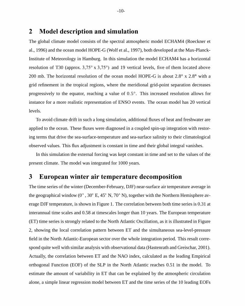
3 European winter air temperature decompositionThe time series of the winter (December-February, DJF) near-surface air temperature average in

the geographical window (0�

, 30�

E, 45�

N, 70�

N), together with the Northern Hemisphere av-

erage DJF temperature, is shown in Figure 1. The correlation between both time series is 0.31 at

interannual time scales and 0.58 at timescales longer than 10 years. The European temperature

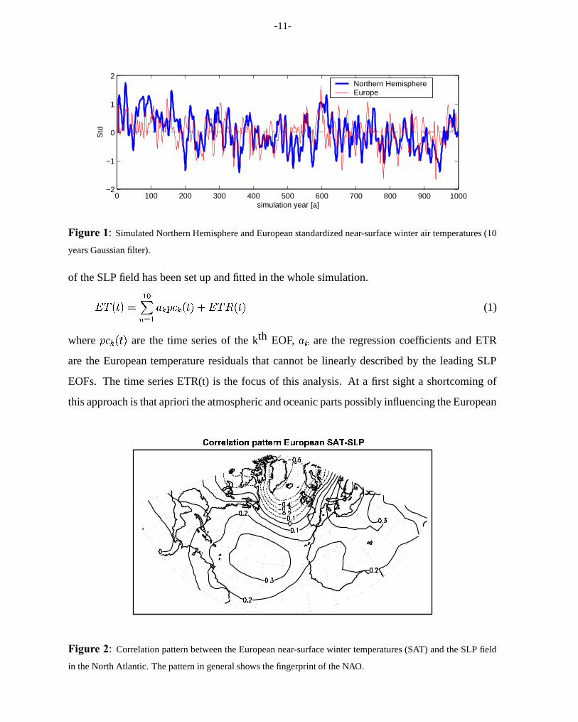
(ET) time series is strongly related to the North Atlantic Oscillation, as it is illustrated in Figure

2, showing the local correlation pattern between ET and the simultaneous sea-level-pressure

field in the North Atlantic-European sector over the whole integration period. This result corre-

spond quite well with similar analysis with observational data (Hastenrath and Greischar, 2001).

Actually, the correlation between ET and the NAO index, calculated as the leading Empirical

orthogonal Function (EOF) of the SLP in the North Atlantic reaches 0.51 in the model. To

estimate the amount of variability in ET that can be explained by the atmospheric circulation

alone, a simple linear regression model between ET and the time series of the 10 leading EOFs

-11-

0 100 200 300 400 500 600 700 800 900 1000−2

−1

0

1

2

simulation year [a]

Std

Northern HemisphereEurope

Figure 1: Simulated Northern Hemisphere and European standardized near-surface winter air temperatures (10

years Gaussian filter).

of the SLP field has been set up and fitted in the whole simulation.

�� (1)

where ��!� �� are the time series of the kth EOF, �� are the regression coefficients and ETR

are the European temperature residuals that cannot be linearly described by the leading SLP

EOFs. The time series ETR(t) is the focus of this analysis. At a first sight a shortcoming of

this approach is that apriori the atmospheric and oceanic parts possibly influencing the European

"$#&%�%('*) +!,�- #/.10�+�,2,('3%�.54�67%8#&09':+*.;/<>=@?(;BA3C

Figure 2: Correlation pattern between the European near-surface winter temperatures (SAT) and the SLP field

in the North Atlantic. The pattern in general shows the fingerprint of the NAO.

-12-

� � ��

�

��

��

��! �"$#&%��('

)�*)*)* )*

+ � , - . � +� +0/ �

+�/ +

+�/ �

+�/ �

+�/ 1

2 �34� ��65��

��! �"7#&%��('

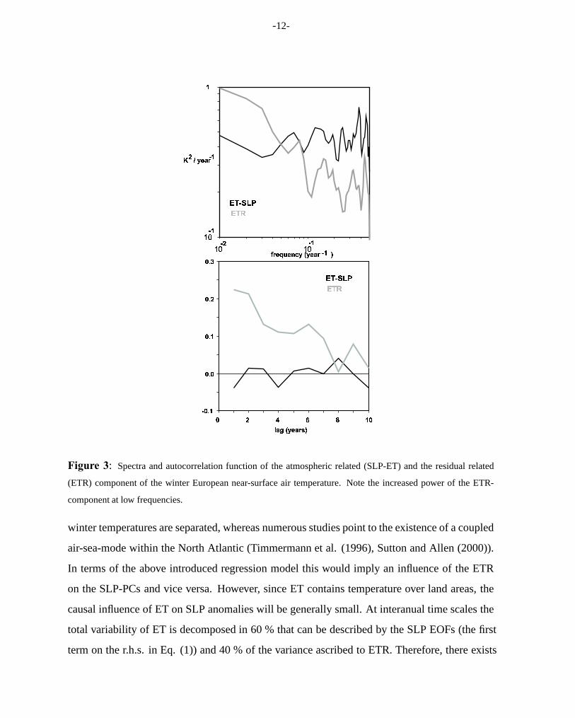
Figure 3: Spectra and autocorrelation function of the atmospheric related (SLP-ET) and the residual related

(ETR) component of the winter European near-surface air temperature. Note the increased power of the ETR-

component at low frequencies.

winter temperatures are separated, whereas numerous studies point to the existence of a coupled

air-sea-mode within the North Atlantic (Timmermann et al. (1996), Sutton and Allen (2000)).

In terms of the above introduced regression model this would imply an influence of the ETR

on the SLP-PCs and vice versa. However, since ET contains temperature over land areas, the

causal influence of ET on SLP anomalies will be generally small. At interanual time scales the

total variability of ET is decomposed in 60 % that can be described by the SLP EOFs (the first

term on the r.h.s. in Eq. (1)) and 40 % of the variance ascribed to ETR. Therefore, there exists

-13-

a substantial amount of temperature interannual variance that is still linearly independent of the

atmospheric circulation as represented by the SLP field. At longer time scales the amount of

variance described by ETR increases. For example, at timescales longer than 10 years the ET

variance is decomposed in 35 % for the SLP-dependent part (hereafter SLP-ET) and 55 % for

ETR. Hence, at these timescales the SLP-independent contribution to ET is dominant. This is

illustrated in Figure 3, that shows the autocorrelation function and the spectra of SLP-ET and

ETR. This figure shows that the timescales at which the SLP fingerprint on temperature becomes

weaker than ETR is about 15 years. The spectrum of SLP-ET is essentially white, reflecting

the atmospheric forcing of this temperature component. The spectrum of ETR is white from

high frequencies up to about periods of 10 years and exhibits a weak peak at periods of about

12 years. The persistence of ETR is longer than that of SLP-ET, which exhibits virtually no

persistence, although the interannual autocorrelation of ETR does not attain very high values.

The variability of ETR will not be completely due to a single factor. For instance, all noise

that is not connected to the SLP variability is also contained in ETR. However, several features

indicate that ETR is associated to real physical mechanisms that act on longer scales. The

correlation of ETR with the Northern Hemisphere average temperature is larger than in the case

of SLP-ET: 0.40 at interannual timescales and 0.65 and timescales longer than 10 years. To

gain insight into the nature of these processes the associated correlation patterns between ETR

and the North Hemisphere temperature, sea-surface-temperature (SST) and SLP are shown in

Figure 4.

For comparison purposes the same correlation patterns are shown for the circulation de-

pendent component SLP-ET. The temperature regression patterns associated with SLP-ET and

ETR show clear differences, whereas the temperature linked to SLP-ET shows the well-known

fingerprint of the North Atlantic Oscillation, with warmer than normal temperatures in Western

Europe and colder than normal in Greenland (known as ”Greenland below” in NAO terminol-

ogy). The temperature associated with ETR shows the same sign over Northwestern Europe

and the North Atlantic ocean, with negligible anomalies elsewhere. The amount of tempera-

ture variance described by these two patterns is 12 % and 8 %, respectively, although they are

not orthogonal to each other and, therefore, some part of the described variance is common to

both. For SST similar results are obtained. The pattern related to SLP-ET shows the tripo-

-14-

��

��

�� !��

"�#%$'&(#*),+�".-/),#0)1#32/4657-(+/892:�;/<>= ),#/8?+�"1#@5A"1#%$'&(#*),+�".-/),#

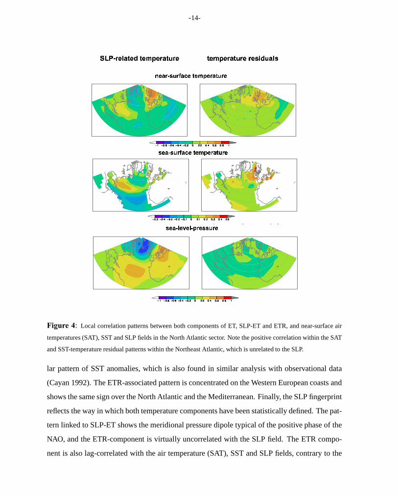
Figure 4: Local correlation patterns between both components of ET, SLP-ET and ETR, and near-surface air

temperatures (SAT), SST and SLP fields in the North Atlantic sector. Note the positive correlation within the SAT

and SST-temperature residual patterns within the Northeast Atlantic, which is unrelated to the SLP.

lar pattern of SST anomalies, which is also found in similar analysis with observational data

(Cayan 1992). The ETR-associated pattern is concentrated on the Western European coasts and

shows the same sign over the North Atlantic and the Mediterranean. Finally, the SLP fingerprint

reflects the way in which both temperature components have been statistically defined. The pat-

tern linked to SLP-ET shows the meridional pressure dipole typical of the positive phase of the

NAO, and the ETR-component is virtually uncorrelated with the SLP field. The ETR compo-

nent is also lag-correlated with the air temperature (SAT), SST and SLP fields, contrary to the

-15-

��

��

��

�

�

�

��

� !" #$$% &$

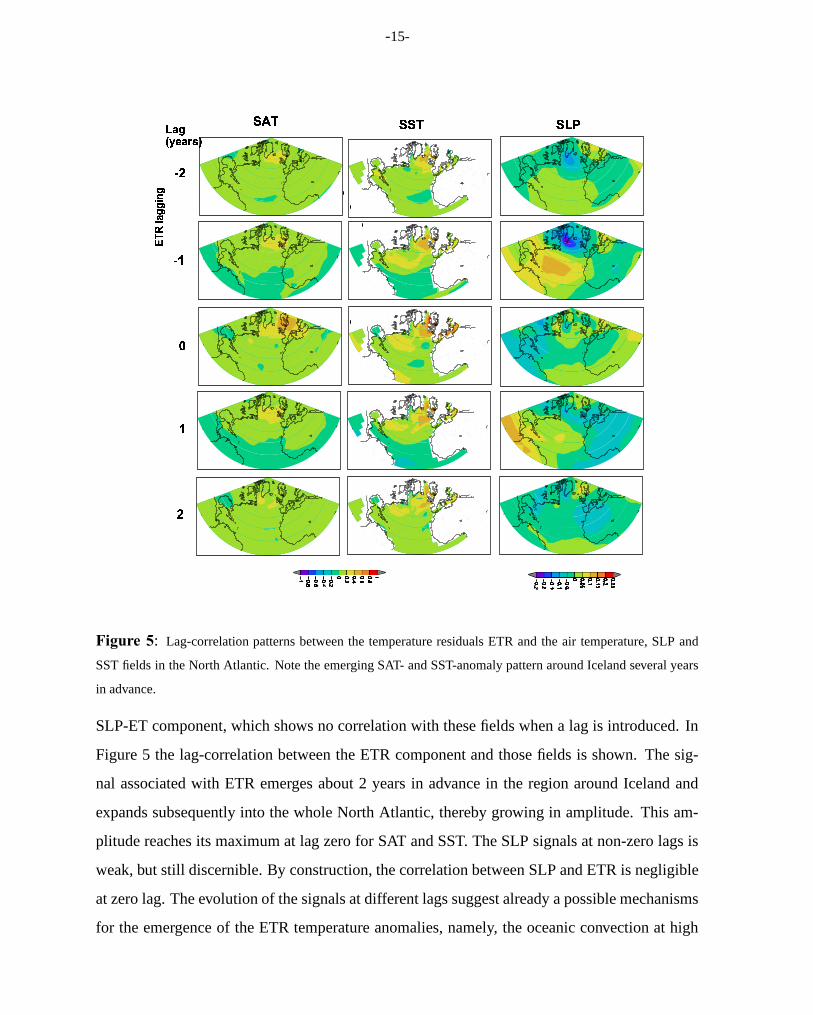
Figure 5: Lag-correlation patterns between the temperature residuals ETR and the air temperature, SLP and

SST fields in the North Atlantic. Note the emerging SAT- and SST-anomaly pattern around Iceland several years

in advance.

SLP-ET component, which shows no correlation with these fields when a lag is introduced. In

Figure 5 the lag-correlation between the ETR component and those fields is shown. The sig-

nal associated with ETR emerges about 2 years in advance in the region around Iceland and

expands subsequently into the whole North Atlantic, thereby growing in amplitude. This am-

plitude reaches its maximum at lag zero for SAT and SST. The SLP signals at non-zero lags is

weak, but still discernible. By construction, the correlation between SLP and ETR is negligible

at zero lag. The evolution of the signals at different lags suggest already a possible mechanisms

for the emergence of the ETR temperature anomalies, namely, the oceanic convection at high

-16-

0 100 200 300 400 500 600 700 800 900 1000−3

−2

−1

0

1

2

3

simulation year [a]

Std

meridional overturningGulf Stream intensity

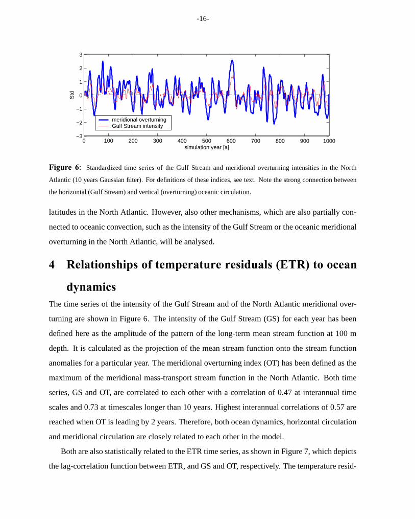
Figure 6: Standardized time series of the Gulf Stream and meridional overturning intensities in the North

Atlantic (10 years Gaussian filter). For definitions of these indices, see text. Note the strong connection between

the horizontal (Gulf Stream) and vertical (overturning) oceanic circulation.

latitudes in the North Atlantic. However, also other mechanisms, which are also partially con-

nected to oceanic convection, such as the intensity of the Gulf Stream or the oceanic meridional

overturning in the North Atlantic, will be analysed.

4 Relationships of temperature residuals (ETR) to ocean

dynamicsThe time series of the intensity of the Gulf Stream and of the North Atlantic meridional over-

turning are shown in Figure 6. The intensity of the Gulf Stream (GS) for each year has been

defined here as the amplitude of the pattern of the long-term mean stream function at 100 m

depth. It is calculated as the projection of the mean stream function onto the stream function

anomalies for a particular year. The meridional overturning index (OT) has been defined as the

maximum of the meridional mass-transport stream function in the North Atlantic. Both time

series, GS and OT, are correlated to each other with a correlation of 0.47 at interannual time

scales and 0.73 at timescales longer than 10 years. Highest interannual correlations of 0.57 are

reached when OT is leading by 2 years. Therefore, both ocean dynamics, horizontal circulation

and meridional circulation are closely related to each other in the model.

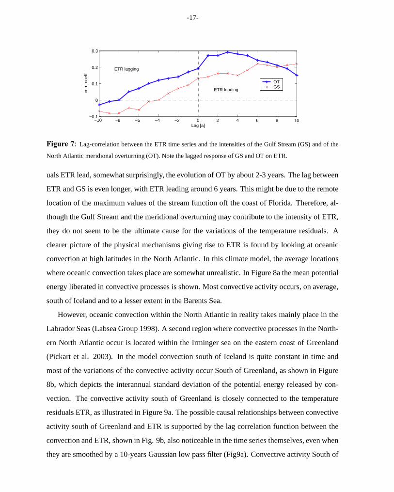
Both are also statistically related to the ETR time series, as shown in Figure 7, which depicts

the lag-correlation function between ETR, and GS and OT, respectively. The temperature resid-

-17-

−10 −8 −6 −4 −2 0 2 4 6 8 10−0.1

0

0.1

0.2

0.3

Lag [a]

corr

. coe

ffOTGS

ETR leading

ETR lagging

Figure 7: Lag-correlation between the ETR time series and the intensities of the Gulf Stream (GS) and of the

North Atlantic meridional overturning (OT). Note the lagged response of GS and OT on ETR.

uals ETR lead, somewhat surprisingly, the evolution of OT by about 2-3 years. The lag between

ETR and GS is even longer, with ETR leading around 6 years. This might be due to the remote

location of the maximum values of the stream function off the coast of Florida. Therefore, al-

though the Gulf Stream and the meridional overturning may contribute to the intensity of ETR,

they do not seem to be the ultimate cause for the variations of the temperature residuals. A

clearer picture of the physical mechanisms giving rise to ETR is found by looking at oceanic

convection at high latitudes in the North Atlantic. In this climate model, the average locations

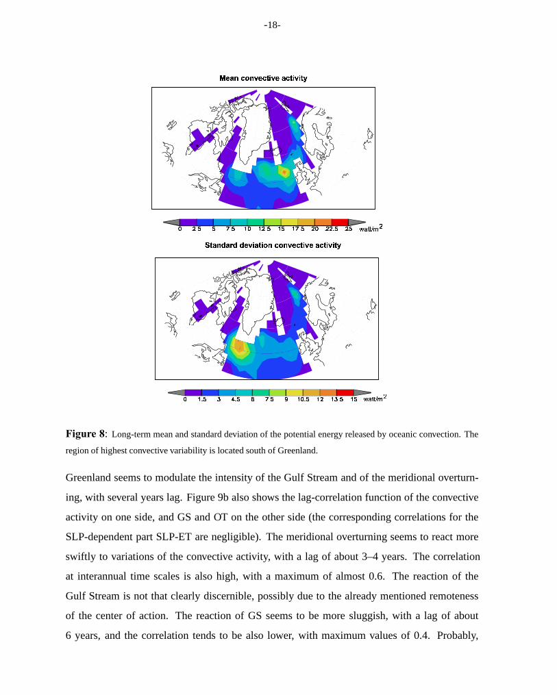
where oceanic convection takes place are somewhat unrealistic. In Figure 8a the mean potential

energy liberated in convective processes is shown. Most convective activity occurs, on average,

south of Iceland and to a lesser extent in the Barents Sea.

However, oceanic convection within the North Atlantic in reality takes mainly place in the

Labrador Seas (Labsea Group 1998). A second region where convective processes in the North-

ern North Atlantic occur is located within the Irminger sea on the eastern coast of Greenland

(Pickart et al. 2003). In the model convection south of Iceland is quite constant in time and

most of the variations of the convective activity occur South of Greenland, as shown in Figure

8b, which depicts the interannual standard deviation of the potential energy released by con-

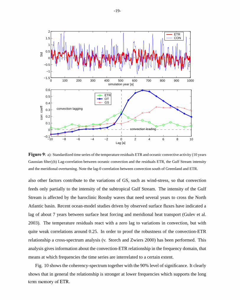
vection. The convective activity south of Greenland is closely connected to the temperature

residuals ETR, as illustrated in Figure 9a. The possible causal relationships between convective

activity south of Greenland and ETR is supported by the lag correlation function between the

convection and ETR, shown in Fig. 9b, also noticeable in the time series themselves, even when

they are smoothed by a 10-years Gaussian low pass filter (Fig9a). Convective activity South of

-18-

��

� ��

!#"%$ $ &('*)

!#"%$ $ &(' )

Figure 8: Long-term mean and standard deviation of the potential energy released by oceanic convection. The

region of highest convective variability is located south of Greenland.

Greenland seems to modulate the intensity of the Gulf Stream and of the meridional overturn-

ing, with several years lag. Figure 9b also shows the lag-correlation function of the convective

activity on one side, and GS and OT on the other side (the corresponding correlations for the

SLP-dependent part SLP-ET are negligible). The meridional overturning seems to react more

swiftly to variations of the convective activity, with a lag of about 3–4 years. The correlation

at interannual time scales is also high, with a maximum of almost 0.6. The reaction of the

Gulf Stream is not that clearly discernible, possibly due to the already mentioned remoteness

of the center of action. The reaction of GS seems to be more sluggish, with a lag of about

6 years, and the correlation tends to be also lower, with maximum values of 0.4. Probably,

-19-

0 100 200 300 400 500 600 700 800 900 1000−1.5

−1

−0.5

0

0.5

1

1.5

2

simulation year [a]

Std

ETR CON

−10 −8 −6 −4 −2 0 2 4 6 8 10−0.1

0

0.1

0.2

0.3

0.4

0.5

0.6

Lag [a]

corr

. coe

ff

ETROTGS

convection lagging

convection leading

Figure 9: a): Standardized time series of the temperature residuals ETR and oceanic convective activity (10 years

Gaussian filter);b) Lag-correlation between oceanic convection and the residuals ETR, the Gulf Stream intensity

and the meridional overturning. Note the lag-0 correlation between convection south of Greenland and ETR.

also other factors contribute to the variations of GS, such as wind-stress, so that convection

feeds only partially to the intensity of the subtropical Gulf Stream. The intensity of the Gulf

Stream is affected by the baroclinic Rossby waves that need several years to cross the North

Atlantic basin. Recent ocean-model studies driven by observed surface fluxes have indicated a

lag of about 7 years between surface heat forcing and meridional heat transport (Gulev et al.

2003). The temperature residuals react with a zero lag to variations in convection, but with

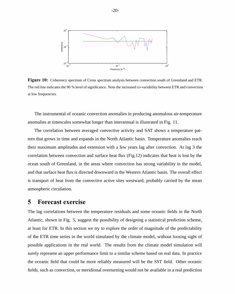
quite weak correlations around 0.25. In order to proof the robustness of the convection-ETR

relationship a cross-spectrum analysis (v. Storch and Zwiers 2000) has been performed. This

analysis gives information about the convection-ETR relationship in the frequency domain, that

means at which frequencies the time series are interrelated to a certain extent.

Fig. 10 shows the coherency-spectrum together with the 90% level of significance. It clearly

shows that in general the relationship is stronger at lower frequencies which supports the long

GAST

term memory of ETR.

-20-

10−2

10−1

100

10−2

10−1

100

frequency [a−1]

cohe

renc

y

Figure 10: Coherency spectrum of Cross spectrum analysis between convection south of Greenland and ETR.

The red line indicates the 90 % level of significance. Note the increased co-variability between ETR and convection

at low frequencies.

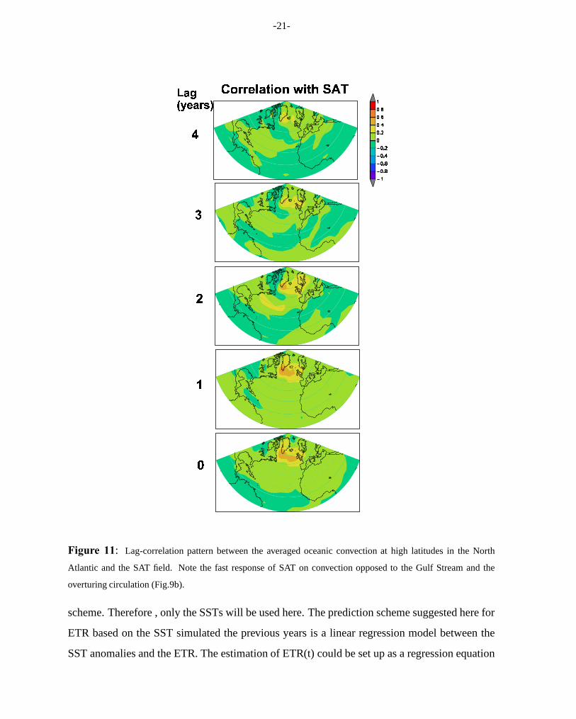
The instrumental of oceanic convection anomalies in producing anomalous air-temperature

anomalies at timescales somewhat longer than interannual is illustrated in Fig. 11.

The correlation between averaged convective activity and SAT shows a temperature pat-

tern that grows in time and expands in the North Atlantic basin. Temperature anomalies reach

their maximum amplitudes and extension with a few years lag after convection. At lag 3 the

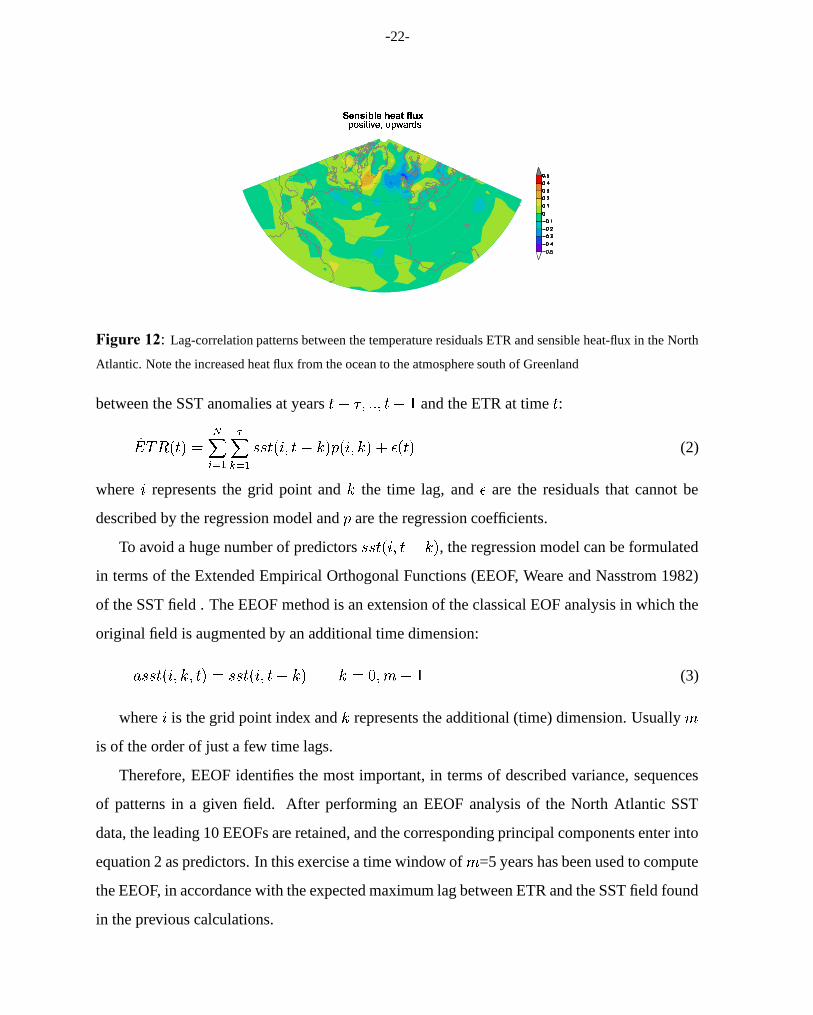
correlation between convection and surface heat flux (Fig.12) indicates that heat is lost by the

ocean south of Greenland, in the areas where convection has strong variability in the model,

and that surface heat flux is directed downward in the Western Atlantic basin. The overall effect

is transport of heat from the convective active sites westward, probably carried by the mean

atmospheric circulation.

5 Forecast exerciseThe lag correlations between the temperature residuals and some oceanic fields in the North

Atlantic, shown in Fig. 5, suggest the possibility of designing a statistical prediction scheme,

at least for ETR. In this section we try to explore the order of magnitude of the predictability

of the ETR time series in the world simulated by the climate model, without loosing sight of

possible applications in the real world. The results from the climate model simulation will

surely represent an upper performance limit to a similar scheme based on real data. In practice

the oceanic field that could be more reliably measured will be the SST field. Other oceanic

fields, such as convection, or meridional overturning would not be available in a real prediction

-21-

��

�

�

�

�

�

�� "!��#%$&!'��(*),+.-

Figure 11: Lag-correlation pattern between the averaged oceanic convection at high latitudes in the North

Atlantic and the SAT field. Note the fast response of SAT on convection opposed to the Gulf Stream and the

overturing circulation (Fig.9b).

scheme. Therefore , only the SSTs will be used here. The prediction scheme suggested here for

ETR based on the SST simulated the previous years is a linear regression model between the

SST anomalies and the ETR. The estimation of ETR(t) could be set up as a regression equation

-22-

�� "!$#&% '��

Figure 12: Lag-correlation patterns between the temperature residuals ETR and sensible heat-flux in the North

Atlantic. Note the increased heat flux from the ocean to the atmosphere south of Greenland

between the SST anomalies at years�)(+* ,$-.-/, �0(21

and the ETR at time�:

3�� 4�5 � �

6��

787 � ��9 , �:(<; � � ��9 , ;B� �>=��(2)

where9

represents the grid point and;

the time lag, and=

are the residuals that cannot be

described by the regression model and � are the regression coefficients.

To avoid a huge number of predictors 787� ��9 , �:(<; �

, the regression model can be formulated

in terms of the Extended Empirical Orthogonal Functions (EEOF, Weare and Nasstrom 1982)

of the SST field . The EEOF method is an extension of the classical EOF analysis in which the

original field is augmented by an additional time dimension:

� 7?7 � ��9 , ; , �� 7?7 � ��9 , �0(>;B� ; A@ ,CB (21(3)

where9

is the grid point index and;

represents the additional (time) dimension. Usually B

is of the order of just a few time lags.

Therefore, EEOF identifies the most important, in terms of described variance, sequences

of patterns in a given field. After performing an EEOF analysis of the North Atlantic SST

data, the leading 10 EEOFs are retained, and the corresponding principal components enter into

equation 2 as predictors. In this exercise a time window of B =5 years has been used to compute

the EEOF, in accordance with the expected maximum lag between ETR and the SST field found

in the previous calculations.

-23-

The regression model can therefore be rewritten as:

3�� =:��

(4)

where � 5 are the regression coefficients, � �� 5 are the principal components of the EEOF. Note

that in eq. 4 � �� 5 (t) contains information from the SST field at time�

and at� ( 1 , � (�� , � (� , � (� ,

since they are the result of projection the EEOF patterns onto the augmented field:

� ��

4�5 � �

787 � ��9 , �0(>;B� � � �� 9 , ;B� (5)

To calibrate the prediction scheme, only data from the first 500 years of the simulation have

been used in all steps: calculation of the EEOF, calculation of their principal components � �$� �� ,and estimation of the regression coefficients � � .

The model is then validated in the last 500 years of the simulation. To keep this prediction

exercise realistic, the estimation of the predicted ETR at time�

should not use any information

of the SST field available at time�, but only information available in previous times. This is

achieved by eliminating the term; @

in the right-hand-side of eq. 5:

3� ��

4�5 � �

787 � ��9 , �0(>;B� � � �� 9 , ;B� (6)

Therefore, the EEOF patterns are truncated in the time dimension to exclude information

from simultaneous time. Formally this truncation is also common in applications of classical

EOF analysis. For instance, EOF patterns may have been calculated in a certain calibration

period and the associated principal components are estimated in another period, when observa-

tions may be more sparse: the grid-points corresponding to missing values are then excluded

from the calculation of the associated principal component.

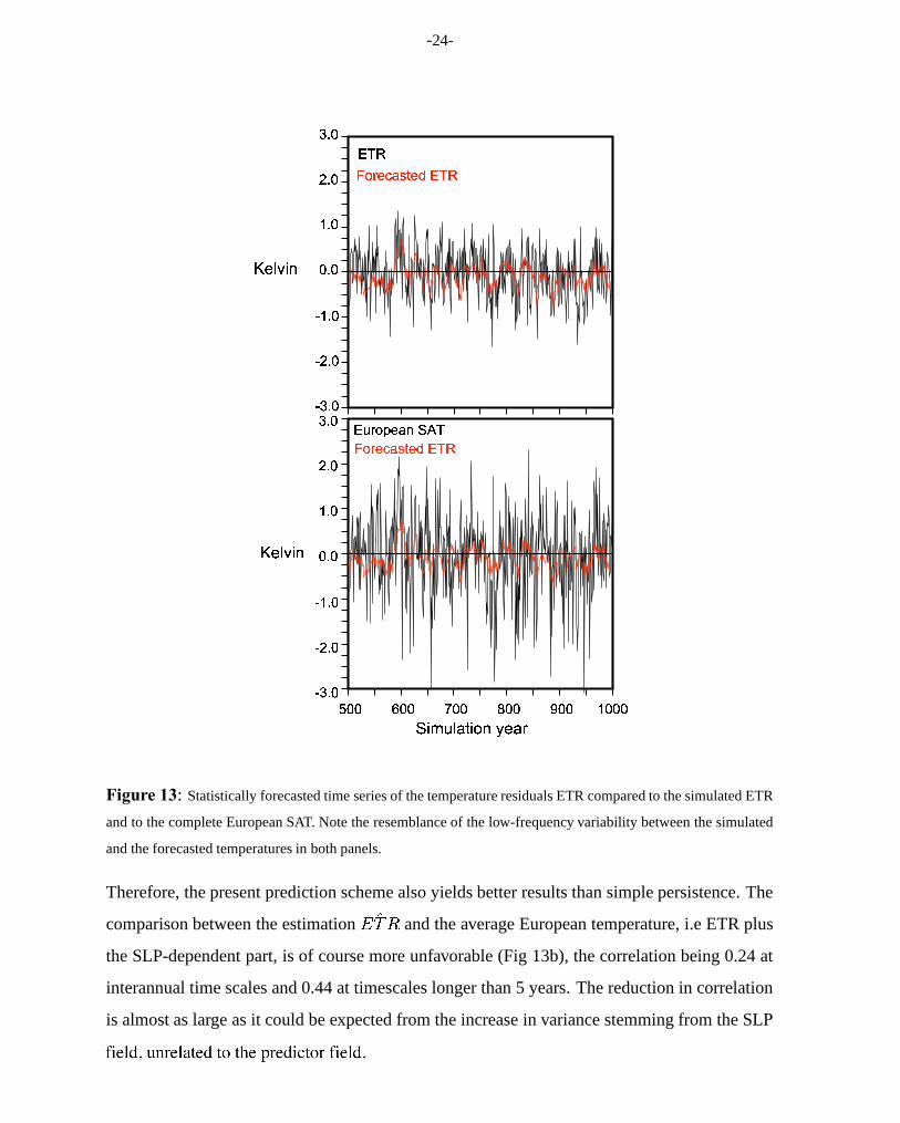
The final estimation of ETR(t) is then carried out by inserting the estimated values3� ��

into equation 4. The results of this prediction exercise is illustrated in Figure 13a, where the

simulated and estimated ETR(t) in the validation period are shown. The correlation between

both is 0.38 at interannual timescales and 0.58 at timescales longer than 5 years. The correla-

tion is admittedly low, specially at interannual timescales, but considering that the prediction

scheme uses only information available in the previous winter, it may be encouraging. This

correlation is also higher than the autocorrelation at lag 1 of the ETR time series, which is 0.23.

-24-

� ��

��

��

��

� � �

� � �

��

��

��

��

��

� � �

� � �

��

�� !#"$��%&��

�('��$�*)+��,.-0/1��*�$�� !#"$��%2��

3.46587:9 ;0<=4 >1?A@�B:;1C

D BE9 F:46?

D BE9 F:46?

Figure 13: Statistically forecasted time series of the temperature residuals ETR compared to the simulated ETR

and to the complete European SAT. Note the resemblance of the low-frequency variability between the simulated

and the forecasted temperatures in both panels.

Therefore, the present prediction scheme also yields better results than simple persistence. The

comparison between the estimation3� � �

and the average European temperature, i.e ETR plus

the SLP-dependent part, is of course more unfavorable (Fig 13b), the correlation being 0.24 at

interannual time scales and 0.44 at timescales longer than 5 years. The reduction in correlation

is almost as large as it could be expected from the increase in variance stemming from the SLP

GAST

GAST

GAST

field, unrelated to the predictor field.

-25-

6 Concluding remarksIn this climate simulation with the climate model ECHO-G the amount of variance of European

winter air temperature that is related to the SLP field is about half of the total variance at decadal

timescales. The origin of most of this variability seems to be related to the convective activity in

the North Atlantic ocean. Since the observational record is too sparse and too short to ascertain

if this is also the case in the real world, simulations with other models should be analyzed.

If these results can be translated to the real world, some consequences could be derived per-

taining paleoclimatic reconstructions and long-term climate prediction. Concerning the latter,

temperature proxies are often used as indicators of past atmospheric circulation anomalies, due

to the, at interannual timescales, strong connection between European winter temperatures and

the North Atlantic Oscillation. This relationship may weaken at longer timescales due to the

effect of other external factors influencing temperature, such as variations in external radiative

forcing. If the model results presented here can be applied to the real world, the contribution

to air temperature in continental areas may be affected at decadal time scales by other internal

factors of the climate systems, that are not directly connected to the atmospheric circulation.

The interpretation of the proxy signal as being completely caused by atmospheric circulation

anomalies may potentially lead to reconstructions with a non-negligible error (see Fig. 4).

The associated temperature anomaly patterns over continental areas are difficult to differentiate

from each other, and only the temperature see-saw between Europe and Greenland would imply

a clear temperature fingerprint of the direct influence of SLP.

The origin of oceanic convection anomalies, that in turn modulate a part of the European

temperature, has not been the focus of this study. Numerous modelling and observational stud-

ies link decadal variations of the thermohaline circulation and oceanic convection in the North

Atlantic at high latitudes to one or several physical mechanisms: a coupled atmosphere-ocean

mode, an ocean-alone or be just a oceanic response to atmospheric forcing. These mechanisms

may involve sea-ice export from the Arctic Ocean (Lohmann and Gerdes 1998; Holland et

al. 2001), fresh water fluxes (Mysak 1990), heat fluxes associated to atmospheric circulation

anomalies (Eden and Jung 2001), or water density anomalies advected by ocean currents (Del-

GAST

GAST

-26-

worth et al. 1993; Hakinnen 2000). The spectrum of ETR (see Fig. 3) shows a peak at about

12 years that might be an indication of the existence of a quasi-oscillatory mode. Although the

time series of the temperature residuals ETR has been constructed so that it contains no infor-

mation of the simultaneous SLP field, it cannot be ruled out that lagged relationships between

large-scale atmospheric forcing and the oceanic circulation my be involved in the generation

of the convection anomalies. ( Pickart et al. 2003). For the purpose of this model study, how-

ever, it was shown that on decadal and secular timescales the low frequency oceanic variability

may act as a pacemaker, possibly pre-conditioning the long term European winter temperature

anomalies.

Acknowledgments. We thank C. Matulla and M. Montoya for their help at improving the

manuscript. The help of the ’Arbeitsgruppe Klimaforschung’ of the Institute of Geography

at the University of Wurzburg is also much appreciated. The climate simulation was carried out

at the German Climate Computing Center (DKRZ).

-27-

ReferencesCayan D (1992) Latent and sensible heat-flux anomalies over the Northern Oceans - the con-

nection to the monthly atmospheric circulation. J Clim 5:354–369

Cook ER, D’Arrigo RD, Mann ME (2002) A well verified, multiproxy reconstruction of the

Winter North Atlantic Oscillation Index since A.D. 1400. J Clim 15:1574–1764

Delworth T, Greatbach R (2000) Multidecadal thermohaline circulation variability driven by

atmospheric surface flux forcing. J Clim 13:1481–1495

Delworth T, Manabe S, Stouffer RJ (1993) Interdecadal Variations of the Thermohaline Cir-

culation in a Coupled Ocean-Atmosphere Model. J Clim 6:1993–2011

Eden C, Willebrand J (2001) Mechanisms of interannual to decadal variability of the North

Atlantic circulation, J Clim 14:2266–2280

Glueck MF, Stockton CW (2001) Reconstruction of the North Atlantic Oscillation, 1429-1983.

Int J Climatol 21:1453–1465

Gulev SK, Barnier B, Knochel H, Molines JM, Cottet M (2003) Water Mass Transformation in

the North Atlantic and Its Impact on the Meridional Circulation: Insights from an Ocean

Model Forced by NCEP-NCAR Reanalysis Surface Fluxes. J Clim 16:3085–3110

Hakkinen S (2000) Decadal Air-Sea Interaction in the North Atlantic Based on Observations

and Modeling Results. J Clim 13:1195–1219

Hastenrath S, Greischar L (2001) The North Atlantic Oscillation in the NCEP-NCAR reanal-

ysis. J Clim 14:2404–2413

Holland MM, Bitz CM, Eby M, Weaver AJ (2001) The Role of Ice-Ocean Interactions in the

Variability of the North Atlantic Thermohaline Circulation. J Clim 14:656-675

Johansson A, Barnston AG, Saha S, van den Dool HM (1998) On the level of seasonal forecast

skill in northern Europe. J Atmos Sci 55:103–127

-28-

Labsea Group (1998) The Labrador Sea deep convection experiment. Bull Am Meteorol Soc

79:2033–2058

Latif M (2000) Dynamics of interdecadal variability in coupled atmosphere-ocean modes. J

Clim 11:602–624

Latif M, Arpe K, Roeckner E (2000) Oceanic control of decadal North Atlantic sea level

pressure variability in winter. Geophys Res Lett 27:727–730

Latif, M Barnett TP (1994) Causes of decadal climate variability over the North Pacific and

North America. Science 266:634–637

Legutke S, Voss R(1999) The Hamburg Atmosphere-Ocean Coupled Circulation Model ECHO-

G. Technical Report No. 18, German Climate Computer Center (DKRZ)

Lohmann G, Gerdes R (1998) Sea Ice Effects on the Sensitivity of the Thermohaline Circula-

tion. J Clim 11:2789–2803

Luterbacher J, Xoplaki E, Dietrich D, Rickli R, Jacobeit J, Beck C, Gyalistras D, Schmutz

C, Wanner H, (2002) Reconstruction of Sea Level Pressure fields over the Eastern North

Atlantic and Europe back to 1500. Clim Dyn 18:545–561

Mysak LA, Manak DK, Marsden RF (1990) Sea-ice anomalies observed in the Greenland

and Labrador Seas during 1901–1984 and their relation to an interdecadal Arctic climate

cycle. Clim Dyn 5:111–133

Paeth H, Latif M, Hense A (2003) Global SST influence on twentieth century NAO variability.

Clim Dyn 21:63–75.

Pickart RS, Spall AS, Ribergaard MH, Moore GWK, Milliff RF (2003) Deep convection in

the Irminger Sea forced by the Greenland tip jet. Nature 424:152–156

Rahmstorf S, Ganopolski S (1999) Long-term global warming scenarios computed with an

efficient coupled climate model. Climatic Change 43:353–367

-29-

Rodwell MJ, Rowell DP, Folland CK (1999) Oceanic forcing of the wintertime North Atlantic

Oscillation and European climate. Nature 398:320–323

Roeckner E, Arpe K, Bengtsson L, Christoph M, Claussen M, Dumenil L, Esch M, Gior-

getta M, Schlese U, Schulzweida U (1996) The atmospheric general circulation model

ECHAM4: Model description and simulation of present-day climate. Rep 218, Max-

Planck-Institut fur Meteorologie, Bundesstr 55, Hamburg, Germany

Seager R, Battisti DS, Yin J, Gordon N, Naik N, Clement AC, Cane MA (2003) Is the Gulf

Stream responsible for Europe’s mild winters? Q J R Meteor Soc 128:2563–2586

Stephenson DB, Pavan V, Bojariu R (2000) Is the North Atlantic Oscillation a random walk?

Int J Climatol 20:1–18

Sutton RT, Allen MR (1997) Decadal predictability of North Atlantic sea surface temperature

and climate. Nature 388:563–567

Timmermann A, Latif M, Voss R, Grotzner A (1996) North Atlantic interdecadal variability:

a coupled air-sea mode. J Clim 11:522–534

von Storch H, Zwiers FW (1999) Statistical analysis in climate research. Cambridge Univer-

sity Press, Cambridge, pp 484

Wanner H , Bronnimann S, Casty C, Gyalistras D, Luterbacher J, Schmutz C, Stephenson DB,

Xoplaki E (2001) North Atlantic Oscillation - Concepts and Studies. In: Rycroft, MJ

(ed), Surveys in Geophysics 22, Kluwer Academic Publishers, pp 321–382

Weare BC, Nasstrom, JN (1982) Examples of extended empirical orthogonal function analysis.

Mon Wea Rev 110:481–485

Wolff JO, Maier-Reimer E, Legutke S (1997) The Hamburg Ocean Primitive Equation Model,

Technical Report No 13, German Climate Computer Center (DKRZ), Hamburg

Wunsch C (1999) The interpretation of short climate records, with comments on the North

Atlantic Oscillation and Southern Oscillations. Bull Am Meteorol Soc 80:245–255

-30-

Zorita E, Frankignoul C (1997) Modes of North Atlantic Decadal Variability in the ECHAM1/LSG

Coupled Ocean-Atmosphere General Circulation Model. J Clim 10:183–200

Documents

The contribution of ocean dynamics on the variability of