The Contribution of Railways to Economic Growth in Latin America

before 1914: a Growth Accounting Approach

Alfonso Herranz-Loncán

(Universitat de Barcelona)

1

The Contribution of Railways to Economic Growth in Latin America before 1914:

a Growth Accounting Approach1

Abstract

Railways are usually considered as one of the most important innovations that

fostered the transition of Latin America to economic growth before 1914. The

social saving estimates that are available for several Latin American countries

seem to confirm that view. However, the interpretation of the results of the

social saving literature is not straightforward, since the comparison among social

savings calculated for different countries and years may be troublesome, and the

actual meaning of the social saving estimates is not clear. This paper suggests an

alternative approach to the economic impact of railways in Latin America. It

presents estimates of the direct growth contribution of the railway technology in

Argentina, Brazil, Mexico and Uruguay before 1914, which are calculated on the

basis of the growth accounting methodology. The outcomes of the estimation

indicate that railway effects on Uruguayan economic growth were very low. By

contrast, in the other three cases under study (Argentina, Mexico and Brazil) the

railways provided huge direct benefits. In Argentina and Mexico, these

amounted to between one fifth and one quarter of the total income per capita

growth of the period under analysis. By contrast, in the case of Brazil, the

outcomes of the analysis indicate that the direct contribution of railways to

growth would have been higher than the whole income per capita growth of the

Brazilian economy before 1914. This unexpected result might suggest that the

national level is not the most adequate scale to analyse the economic impact of

network infrastructure in the case of large, geographically unequal and

insufficiently integrated developing economies.

1. Introduction

Between the mid nineteenth century and the eve of the Great War, Latin

America was one of the world regions with a faster economic growth. According to

Maddison’s figures, the economies of the area grew well above the world average in

1870-1913, and its growth rate was comparable that of the “Western Offshoots” (Table

1). To a large extent, that growth episode was a consequence of the expansion of

exports of primary products during the first globalisation boom.

1 This research has been financed by the Spanish Ministry of Science and Innovation project ECO2009-

13331-C02-02. I thank Sandra Kuntz, Paolo Riguzzi and the participants at the I Encuentro de la AEHE,

the XXVI Jornadas of the Banco Central del Uruguay, the 2011 Carlos III FRESH Meeting and the 9th

EHES Conference for their comments and help. They are not responsible for the mistakes of the paper.

2

Table 1. Growth rates during the first globalisation boom (1870-1913)

Percentage points per year GDP GDP per

capita

Latin America 3.48 1.81

Western Europe 2.10 1.32

Western Offshoots 3.92 1.81

Japan 2.44 1.48

Asia (excluding Japan) 0.94 0.38

Eastern Europe and former USSR 2.37 1.15

Africa 1.40 0.64

World 2.11 1.30

Source: Maddison (2001), p. 126.

In many Latin American economies the construction of railway networks was

one of the most important bases of the economic expansion of 1870-1913. As in the rest

of the world, Latin American railways had a huge influence on the reduction of

domestic transport costs. In addition, in the case of Latin America, and opposite to what

happened in the industrialised economies, which had already developed relatively

efficient and competitive market structures at the advent of the railways, these were

essential to create or to strengthen the links between previously fragmented local

markets, and also between them and the world markets. In this regard, they had a much

more “developmental” character in Latin America than in the core economies

(Coatsworth, 1981, pp. 77-78).

Historians have often highlighted the importance of railways for Latin American

development during the first globalisation. For instance, according to Summerhill

(2003), “the railroad conferred on Brazil benefits that probably exceeded, by far, those

stemming from the other major changes in economic organization in this period” (p.

96), and railways may be considered to have “laid the groundwork for Brazil’s

transition to rapid economic growth after 1900” (p. 1). In the case of Argentina, “[i]n

the aggregate, railroad technology accounted for an appreciable portion of the

productivity growth enjoyed by the Argentine economy between 1890 and 1913.

Railroads were certainly not the sole determinant of overall gains in productivity in the

economy, but they were no doubt among the most important”.2 And, in Mexico, the

railways “were one of the most powerful factors of transition to capitalism”.3 In those

countries, the railways not only generated large increases in aggregate productivity,

thanks to the reduction in transport costs, but also encouraged market integration, labour

2 Summerhill (2000), p. 5; see also Lewis (1983), p. 220.

3 Kuntz Ficker (1999), p. 134; see also Kuntz Ficker (1995) and Dobado and Marrero (2005).

3

mobility, and the emergence of scale and agglomeration economies. In addition, they

increased the economy’s stock of exploitable natural resources, and stimulated the

inflow of foreign capital and the growth of investment. In sum, in Summerhill’s words,

“(…) it now seems unlikely that any other technological or institutional innovation was

more important in the transition to economic growth in Latin America before 1930”

(Summerhill, 2006, p. 297).4

So far attempts to provide quantitative indicators of the economic impact of

Latin American railways have been largely addressed to the estimation of the social

savings, which measure the cost of transporting the railway output of one year by the

best available alternative. Social savings may be considered therefore as an approach to

the resource saving impact of the railway technology, and the high level of Latin

American social saving estimates has usually been interpreted as a clear indicator of the

large contribution of the railway technology to economic growth in the region (see

Table 2).

Table 2. Available estimates of social savings of freight railway transport in several

countries Year Social savings/GNP or GDP (%)

US 1859 3.7

US 1890 4.7

England and Wales 1865 4.1

Russia 1907 4.5

France 1872 5.8

Spain 1878 4.4

Spain 1912 12.7

Colombia 1927 3.37/7.86

Brazil 1913 18.0/38.0

Mexico 1910 24.9/38.5

Argentina 1913 26.0

Sources: Fishlow (1965), pp. 37 and 52; Fogel (1964), p. 223; Hawke (1970), p. 196; Metzer (1977), p.

50; Caron (1983), p. 44; Herranz-Loncán (2008), p. 140; Summerhill (2003), p. 89; Coatsworth (1979), p.

952; Summerhill (2000), p. 31; and Ramírez (2001).

4 Nonetheless, there is also a negative interpretation of the economic role of railways in the Latin

American economies, associated to the dependentista literature. From this perspective, the railways

should be blamed for having promoted and supported a purely extractive economic model, reinforcing the

export orientation of the economies of the region and its dependence on foreign powers, and constituting

therefore an obstacle to the emergence of a different development pattern, more oriented to sustained

economic growth and industrialisation and to the expansion of internal markets. An example of this

approach is Coatsworth (1981, p. 191), who indicates that the railways “may be seen as foreclosing other

[development] possibilities with very large effects over the longer period”, and points out that most of the

benefits of the railway technology were finally channelled to the North-Atlantic economies through the

repatriation of dividends and interest payments and the demand for industrial products. Despite their

relevance, these issues are beyond the scope of this paper.

4

However, these social saving figures cannot be taken as unambiguous indicators

of the relative contribution of railways to economic growth in each country, for two

reasons. Firstly, a direct comparison among social saving estimates calculated for

different years and with different methodologies in order to draw conclusions on the

relative role that railways performed in each economy may be misleading (Leunig,

2010). For instance, since the social savings tend to increase over time, estimates for the

third quarter of the nineteenth century would be hardly comparable with figures for

1914. Secondly, the actual economic meaning of the social saving, as is usually

calculated, is not clear. As has been recently stressed by Leunig (2010), in the case of a

“macro‐invention” (such as the railways), “for which price falls are dramatic, for which

previous levels of quantity sold are relatively small, and for which price elasticity of

demand proves to be high, then it is likely that the social savings estimates will be

hugely out of line with the conventional, and correctly defined, measure used by

economists to value the welfare effects of improvements to technology, namely the rise

in consumer surplus.”

In order to overcome these shortcomings, the growth accounting methodology,

which is actually the most usual way to evaluate the economic growth implications of

new technology over time, may constitute a more adequate approach to the contribution

of railways to economic growth (Crafts, 2010). This paper uses the growth accounting

framework to provide preliminary estimates of the contribution of railways to economic

growth before 1914 in four of the main Latin American economies (Argentina, Brazil,

Mexico and Uruguay), in order to obtain aggregate and comparable indicators of the

direct impact of the railway technology on those economies during the period of export-

led growth. To that purpose, next section offers a brief summary of the process of

railway expansion in Latin America; Section 3 describes the growth accounting

framework that has been used in this paper; Section 4 presents the available evidence on

the growth contribution of railways in Latin America; and, finally, Section 5 concludes.

2. Railways in Latin America before 1914: an overview

By 1914 railways were present all over Latin America, although their

development had been highly unequal among countries. The first railway line in the

region was open in Cuba in 1837, only 12 years after the inauguration of the first British

railway. Cuba would not be joined by any other Latin American economy until the

5

1850s, when railway construction started in Argentina, Brazil, Mexico, Peru, Colombia

and Chile. By 1900, the railways were already present in all countries of the region.

Railway construction was especially intense in Argentina, Brazil and Mexico.

These countries accounted, since the late 1880s, for approximately 75 percent of the

whole Latin American railway mileage. However, in per capita terms, the Brazilian and

Mexican networks fell behind the countries of the Southern Cone, Cuba and Costa Rica,

as may be seen in Tables 3 and 4.

Table 3. Railway mileage in Latin America (1890-1912) (km) 1890 1900 1912

Argentina 9,254 16,767 32,212

Brazil 9,973 15,316 23,491

Mexico 9,718 13,585 20,447

Chile 2,747 4,354 7,260

Cuba 1,731 1,960 3,803

Peru 1,599 1,800 3,276

Uruguay 983 1,730 2,522

Bolivia 209 972 1,284

Colombia 358 644 1,061

Venezuela 454 858 858

Guatemala 186 640 808

Costa Rica 241 388 619

Ecuador 92 92 587

Paraguay 240 240 373

Puerto Rico 18 223 354

Nicaragua 143 225 322

El Salvador 87 116 320

Dominican Republic 115 182 241

Honduras 96 96 170

Haiti 0 37 103

Panama 76

TOTAL 38,244 60,225 100,187

Source: Mitchell (2003).

Note: Panama is included within Colombia both in 1890 and in 1900.

6

Table 4. Railway mileage per capita in Latin America (1890-1912) (km per 10,000 pop)

1890 1900 1912

Argentina 24.39 34.93 42.65

Uruguay 13.90 18.89 21.78

Chile 10.46 14.77 21.20

Costa Rica 10.46 12.64 16.51

Cuba 11.23 12.25 16.13

Mexico 8.25 10.41 14.22

Brazil 6.92 8.34 9.53

Peru 5.99 5.79 7.46

Guatemala 2.33 7.23 7.08

Bolivia 1.04 5.15 6.03

Paraguay 5.96 4.79 5.83

Nicaragua 3.61 4.86 5.67

Ecuador 0.81 0.71 3.81

Venezuela 2.03 3.90 3.31

Dominican Republic 2.60 3.03 3.14

El Salvador 1.29 1.45 3.13

Puerto Rico 0.21 2.33 3.05

Honduras 2.51 2.14 2.96

Colombia 0.89 1.53 2.09

Panama 1.78

Haiti 0 0.29 0.58

TOTAL 7.33 9.94 12.94

Sources: Mitchell (2003), Maddison (2001) and Banks’ CNTS Archive.

Note: Panama is included within Colombia both in 1890 and in 1900.

Tables 3 and 4 may be taken as preliminary evidence of the different role that

railways performed in the growth of each Latin American economy before 1914. In both

tables, Argentina stands out as a special case, where railway expansion reached levels

comparable to some European networks. Other group of economies in which relatively

dense networks were constructed was made up by other Southern Cone countries

(Uruguay and Chile), Cuba, Costa Rica, Mexico and, to some extent, Brazil and Peru.

By contrast, in the rest of the continent railway development was extremely slow and

railway systems were scarcely integrated, consisting mainly of a series of isolated lines

that connected production areas with the main ports, and hardly affecting large shares of

the territory of their countries. Actually, to some extent, the contribution of railways to

the economic growth of each country might be expected to be proportional to the

development of its railway network. In countries with relatively dense networks,

railways would be important not only as a reinforcing factor for the export orientation

of the economy, but also as an instrument of market integration, by its own or in

combination with river and coastal navigation.

This paper focuses on the cases of Argentina, Brazil, Mexico and Uruguay (from

now on, LA4), a sample of countries that, according to Maddison’s database, accounted

7

for 65 percent of Latin American GDP and 59 percent of the region’s population by

1913. These countries are in the first ranks of Tables 3 and 4; they possessed 79 percent

of the total Latin American mileage in 1912 and had, together with Chile, Costa Rica

and Cuba, the highest mileage per capita in the region. Actually, with the exception of

Brazil, they were among the rare cases where an integrated national railway network

was built. A priori, therefore, they might be expected to be among those Latin American

economies in which the railways had a higher growth impact. The next sections try to

approach that impact through the application of growth accounting techniques.

3. The measurement of the contribution of railways to economic growth.

The most usual way to measure the global contribution of technological change

to economic growth is the estimation of the so-called “Solow Residual”, on the basis of

a typical Cobb-Douglas production function and competitive assumptions. The “Solow

residual” (∆A/A) was originally interpreted as the total factor productivity growth

provided by new technology, and is estimated from the following expression:

∆(Y/L)/(Y/L) = sK∆(K/L)/(K/L)+∆A/A (1),

where Y is total output, L is the total number of hours worked, K denotes the services

provided by the capital stock, and sK is the factor income share of capital.

Some recent research on the contribution of information and communication

technologies (ICT) to economic growth has been based on a generalization of

expression (1), which aims at incorporating the hypothesis of endogenous innovation

and embodied technological change. Oliner and Sichel (2002), for instance, apply a

disaggregated version of equation (1), in which different types of capital and different

components of TFP growth are distinguished. This allows them to measure the growth

impact of ICT, both through disembodied TFP growth and through the embodied

capital-deepening effect of investment in ICT. Therefore, they transform expression (1)

into:

∆(Y/L)/(Y/L)=sKo∆(Ko/L)/(Ko/L)+γ(∆A/A)o+sKICT ∆(KICT/L)/(KICT/L)+ϕ (∆A/A)ICT (2)

where KICT and Ko are the services provided by capital stock in ICT and in other sectors,

respectively, A is the TFP level in the sector indicated by the subscript (ICT and other),

sKICT and sKo are the factor income shares of ICT capital and other capital, and ϕ and γ

are the shares of ICT and other sectors’ production in total output.

8

The contribution of a new technology to labor productivity growth may be

approached by the sum of the last two terms of equation (2), which would approach,

respectively, the “capital contribution” and the “TFP contribution” of the new

technology. In fact, this would be a lower bound estimate of the real impact of the new

technology, as there may be spillovers from the sector under consideration to the rest of

the economy that would not be included in that estimate. Unfortunately, growth

accounting studies usually fail to quantify indirect TFP spillovers, due to the

measurement difficulties involved.5

When this methodology is applied to the study of non-leading economies, it is

necessary to introduce an additional caveat. The use of the TFP growth rate in a specific

sector as a measurement of the “TFP contribution” of that sector’s new technology may

be adequate for the analysis of advanced economies, in which new technologies are only

introduced when they can provide their services at the same cost as the old technology

that they replace. For instance, in the case of Britain, the railways were introduced when

they could provide transport services at a similar unit cost to that of their competitors

(mainly waterways and coastal navigation) and, therefore, the contribution of the

railway technology to the aggregate British TFP growth (excluding spillovers) may be

adequately approached by the growth of TFP in the railway sector.

By contrast, that procedure may be misleading in the case of peripheral

countries, which acquire new technologies from the core economies. Peripheral

countries might obtain higher TFP gains from a new technology than those measured by

the TFP growth rate of the corresponding sector, for two reasons. On the one hand, the

old sectors that the new technology was going to replace might be less efficient than in

the core economies. On the other hand, peripheral countries might acquire the new

technology when it had already been used and improved in the leading economies for a

while. As a consequence, at the time of the introduction of the new technology, the

difference between the unit cost of its services and the services provided by the old

technology that it replaces might be very large. In a complete growth accounting

assessment, the “TFP contribution” of a new technology should include that difference,

and TFP growth in the new technology sector would therefore not provide a complete

measure for that contribution.

5 See Oliner and Sichel (2002), pp. 16-20, and Crafts (2004b), pp. 339-340.

9

This issue was already stressed in Herranz-Loncán (2006) for the case of the

Spanish railways. Whereas, as has already been indicated, the first British railways had

no great cost advantage over their main competitor (i.e. water transportation) when they

were established, the first Spanish railway services were considerably cheaper than the

alternative modes they displaced (mainly traditional overland transportation), and the

difference between railway and traditional transport costs should be included in the

contribution of the railways to TFP growth in the Spanish economy (and added up to the

last term of expression 2). Similarly, an estimate of the whole TFP effects of Latin

American railways should not only include TFP improvements within the railway sector

itself (as in the British case) but also those TFP gains that were associated to the shift

from old forms of transportation to the railways (as in the Spanish case).

In this context, instead of approaching the “TFP contribution” of railways in the

LA4 countries through TFP growth in the railway sector, it may be estimated on the

basis of the available social saving estimates, as those included in Table 2 above. Social

savings are usually calculated as:

SS = (PALT – PRW) x QRW (3)

where PRW and PALT are, respectively, the price of railway and counterfactual

(alternative) transport, and QRW is the railway transport output in the reference year.

This expression is actually an upward biased estimate (due to the implicit assumption of

a price-inelastic transport demand) of the equivalent variation consumer surplus

provided by the railways which, if perfect competition in the rest of the economy is

assumed, provides a general equilibrium measure of the entire direct real income gain

obtained from reducing resource cost in transportation (Metzer, 1984; Jara-Díaz, 1986).

As has been stressed by Crafts, the price dual measure of TFP allows

considering such gain in real income as equivalent to the TFP increase provided by the

railways. According to the previous considerations, in a country like Britain, where

railways were only introduced at the point where they could offer transport services at

the same cost as water transportation, it should actually be equivalent to TFP gains in

the railway sector itself (Crafts, 2004a, p. 6). By contrast, in Spain or in the LA4

economies, the total gain in real income (obtained from the social savings estimations)

would not only reflect TFP growth in the railway sector but also those TFP gains

associated with the shift from old forms of transportation to the railways. As a

consequence, estimates of TFP increases based on the Spanish (or Latin American)

10

social savings might be compared with the British figures based on the TFP growth rate

in the railway sector, in order to analyze differences in the whole TFP growth impact of

the railway system (including the substitution among different transport modes).6 This

comparison is carried out, in the cases of Spain and Britain, in Table 5, which presents

the available estimates of the contribution of the railway technology to economic

growth in those two countries as the sum of the two last terms of expression (2).

Table 5. Railways’ Contribution to Growth in Britain and Spain before 1913 Britain

(1830-1850)

Britain

(1850-1870)

Britain

(1870-1910)

Spain

(1850-1912)

a) Railway capital stock per capita growth 22.8 5.9 0.4 4.2

b) Railway profits share in national income 0.6 2.1 2.7 0.86

c) “Capital term” of the railway growth

contribution (a x b) (percentage points per year) 0.14 0.12 0.01 0.036

d) Railway TFP growth 1.9 3.5 1.0 -

e) Railway share in national output 1.0 4.0 6.0 -

f) “TFP term” of the railway growth contribution

(d x e) (percentage points per year) 0.02 0.14 0.06 0.10 / 0.13

a

g) Total gain in real income from railway TFP

growth / Income per capita increase since the

beginning of the railway era (%)

- - - 10.01/12.56 b

h) TFP Spillovers na na na na

i) Total railway contribution (c+f+h) (percentage

points per year) 0.16 0.26 0.07 0.14 / 0.17

j) Railway contribution as % of GDP per capita

growth 14.97 18.85 8.51 13.64/16.19

Sources: Own elaboration from Crafts (2004b) and Herranz-Loncán (2006) and (2008).

Note: (a) Calculated from row g and the income per capita growth rate in 1850-1912; (b) Calculated

directly from the available social savings estimates; na: not available.

In both countries, the railway technology accounted on average for

approximately 13-16 percent of GDP per capita growth in the six/eight decades before

1913. This is indeed a substantial contribution for a single sector. However, the

similarity between the estimates for both countries critically depends on the inclusion of

the resource saving effects of the shift from alternative transport modes to the railways

in the Spanish case. If this shift were not considered, the direct economic impact of

Spanish railways would just amount to approximately 5 to 6 percent of Spanish GDP

per capita growth, i.e. less than half the contribution presented in Table 5. It is also

interesting to see that, although the contribution of railways to Spanish economic

6 Actually, although small, there was also some potential transport cost reduction in Britain from the

substitution of the railways for alternative transport modes; see Hawke (1970). Therefore, an account of

the growth contribution of the British railways such as that in Table 5, which is just based on the increase

in TFP within the railway sector, would contain certain downward bias associated with the exclusion of

those gains, which must be kept in mind in the comparison between the British and the Spanish or LA4

cases.

11

growth was sizeable, it was not significantly higher than the British equivalent figure.

This contrasts with the traditional interpretation on this matter, based on the available

social saving estimates, which considered that railways were more vital in a poor

country like Spain, with fewer opportunities for water transport, than in a rich country

like Britain, well endowed with waterways. As may be seen in row (b) of the table, that

difference was largely overcome by the much higher importance of the railway sector in

the British than in the Spanish economy. Next section applies this methodology to the

estimation of contribution of the railway technology to productivity growth in the LA4

countries, in order to evaluate the role that railways performed in those countries during

the first globalisation boom.

4. The contribution of railways to economic growth in the LA4 countries

before 1914.

As has been described in the previous section, the contribution of railways to

economic growth may be estimated as the sum of two terms. The first is the product of

the growth rate of the railway capital stock per capita times the factor income share of

railway capital (the “capital contribution”). The second is the TFP growth rate in the

transport sector times the share of railway production in total output (the “TFP

contribution”). As has been indicated, this second term may be measured directly,

through the calculation of the direct real income gain obtained by the economy from

reducing resource cost in transportation, on the basis of the social savings. The next two

subsections are devoted to the estimation of those two terms in the LA4 countries before

1914.

4.1. The contribution of railways to economic growth: the capital term.

There are no available estimates of railway capital stock for the LA4 countries

during the second half of the nineteenth century and the first few years of the twentieth

century. Therefore, as is customary in this kind of exercises, I have assumed the

evolution of railway capital to be similar to that of railway mileage. Table 6 shows the

yearly growth rates of railway mileage per capita in the LA4 countries since the start of

the “railway era” until the eve of World War I.7

7 I do not include in the analysis the early years of operation of the railways, when only some very short

stretches with very little traffic were open to the public. Therefore, I start my analysis, in the case of

12

Table 6. Growth rate of railway mileage per capita Country Period considered Railway km per capita

yearly growth rate

(percent)

Argentina 1865-1913 6.36

Brazil 1864-1913 6.25

Mexico 1873-1910 8.61

Uruguay 1874-1913 3.91

Note: Growth rates are estimated by adjusting a log-trend to the mileage data.

Sources: Railway mileage comes from Mitchell (2003), except for Uruguay, for which it has been directly

estimated from the country’s statistical yearbooks. Population has been taken, for Mexico and Brazil,

from the Maddison’s database, for Uruguay, from Bértola (1998), and for Argentina, from Vázquez-

Presedo (1971). Gaps between population data have been filled through geometric interpolation.

In order to estimate the capital term of the growth contribution of the railways in

each country, those rates should be multiplied by the factor income shares of railway

capital, i.e. the average ratios between railway net operating revenues and nominal GDP

throughout the period under consideration. Table 7 presents estimates of the average

ratios between net revenues and GDP in the LA4 countries. These figures must be taken

with certain caution, especially in the cases of Mexico and Brazil, due both to the

scarcity and bad quality of the statistics on railway operation and to the gaps and the

relatively bad quality of the available nominal GDP figures.

Table 7. Average ratio between net railway revenues and nominal GDP in LA4

during the railway era Railway profit share in national income

(net railway revenues/GDP, %)

Argentina (1865-1913) 1.81

Brazil (1864-1913) 0.81

Mexico (1873-1910) 0.91

Uruguay (1874-1913) 0.71

Sources and notes:

a) Argentina. Net revenue data from Dirección General de Ferrocarriles, Estadística de los ferrocarriles

en explotación (1892-1913). Nominal GDP has been taken, for 1900 onwards, from the Oxlad

database. For 1875-1900, I have driven backwards the Oxlad estimates on the basis of the evolution

of real GDP, taken from Della Paolera, Taylor and Bózzoli (2003), and price indices, taken, for 1884-

1900, from Della Paolera, Taylor and Bózzoli (2003), and, for 1875-1884, from Ferreres (2005). For

1865-75 I have estimated nominal GDP on the basis of Prados de la Escosura’s (2009) assumption

that real income per capita grew at a yearly rate of 0.8 percent, the evolution of population (Vázquez-

Presedo, 1971) and the evolution of prices (Ferreres, 2005).

Argentina, in 1865 (when towns as Luján, Mercedes and Chascomús were already connected to Buenos

Aires), in the case of Brazil, in 1864 (year of the connection of Rio de Janeiro with the Vale do Paraíba

through the Dom Pedro II railway), in the case of Mexico, in 1873 (when the Mexico-Veracruz line was

completed) and, in the case of Uruguay, in 1874 (when Montevideo was connected with Durazno). On the

other hand, in the case of Mexico I end the analysis in 1910, to avoid the impact of the Mexican

revolution and to adapt my research to the chronology of Coatsworth’s social saving estimation (see

below).

13

b) Brazil. In the absence of reliable estimates of net revenues of the whole Brazilian railway network, I

have taken the ratios between net revenues and GDP in 1913 provided by Summerhill (2003) and

have driven them backward on the basis of: i) the series of freight gross revenues of a sample of

Brazilian railway lines estimated by Summerhill (2003), under the assumption that the operating ratio

of the Brazilian railways was constant throughout the period under study and the lines of the sample

represented a constant share of the total revenues of the network;8 ii) the evolution of Brazilian

nominal GDP. This has been taken, for 1900 onwards, from the Oxlad database, and, for the period

before 1900 I have driven backwards the Oxlad estimates on the basis of Goldsmith (1986).

c) Mexico. Firstly, I have estimated the amount of net revenues in 1910 on the basis of the gross

revenues of the network, taken from Coatsworth (1981, pp. 42-43), and the operating ratio of the

Ferrocarriles Nacionales, which accounted for two thirds of the network in 1910, taken from

Grunstein Dickter (1996), p. 202. Secondly, I have assumed the evolution of net revenues between

1873 and 1910 to be similar to that of the gross revenues of the network, available in Coatsworth

(1981, pp. 42-43). This means that I assume, as in the case of Brazil, a constant operating ratio in the

Mexican railway network. Nominal GDP data come, for 1900-1913, from Oxlad and, for 1895-1899,

from Estadísticas Históricas de México (http://biblioteca.itam.mx/recursos/ehm.html). Before 1895,

yearly real GDP figures have been obtained from Maddison (2001) through interpolation, and have

been expressed in nominal terms, for 1885-95, on the basis of the evolution of an index of prices in

Mexico City, taken from Estadísticas Históricas de México, and, for 1878-1885, on the basis of the

index of export prices in Coatsworth (1981), p. 42. For 1873-1875 I have assumed that the growth

rate of real and nominal GDP were the same.

d) Uruguay: for net railway revenues, see Herranz-Loncán (forthcoming, b). Nominal GDP is calculated

on the basis of its level in 1955, taken from the official national accounts, and its previous evolution,

as estimated by Bertino and Tajam (1999) and Bértola (1998).

The average ratios between net revenues and GDP in Table 7 clearly show the

outstanding importance of the railway sector in Argentina, compared with the rest.

Actually, the Argentinean ratio between net revenues and GDP was not very far away

from the average British equivalent figures in 1850-1910 (2.52 percent). By contrast,

those ratios seem to have been significantly lower in Brazil, Mexico and Uruguay,

where they would have been much more similar to the equivalent Spanish figure in

1850-1912 (0.86 percent). This provides a first indication of the different importance of

the railway sector in export-led growth episodes during the period, and the prominent

position of Argentina in this regard, as is stressed below.

As a result of those calculations, the capital term of the yearly contribution of

railways to growth in Brazil, Mexico and Uruguay would range between 0.03 and 0.08

percentage points of growth, whereas the capital term of the growth contribution of the

8 It is difficult to know how far away these assumptions are from the real situation of the Brazilian

railways, and they, therefore, may have introduced some biases in the final figures of unknown

magnitude. The sample of lines analysed by Summerhill (2003) accounted for a relatively constant share

of the Brazilian railway mileage only since the mid 1870s (around 55 percent). Before that date, however,

they would represent approximately 80 percent of the total mileage of the network; see Summerhill

(2003), pp. 66-67. If this change is accounted for in the estimation, it hardly affects the final estimates

(the Brazilian figure in Table 7 would be 0.79 instead of 0.81). This correction, however, has not been

applied to the calculation, because the lines excluded from Summerhill’s sample and built after the mid

1870s may be assumed to have lower net revenues per km than the lines of the sample, which were

among the most important of the Brazilian system.

14

Argentinean railways would have been much higher (0.12). With the exception of

Argentina, the reported percentages are in line with the equivalent Spanish figure in

1850-1912 (0.036) and the British estimate for 1830-1910 (ca. 0.07). In this context, the

relative advantage of Argentina was mainly associated to the large size of the railway

sector relative to GDP (see Table 8).

Table 8. The contribution of railways to economic growth in LA4: the capital term (a)

Railway km per capita

yearly growth rate

(percent)

(b)

Railway profit share in

national income

(net railway

revenues/GDP, percent)

(c)

Railway contribution to

economic growth:

capital term

(percentage points of

growth)

(a x b)

Argentina (1865-1913) 6.36 1.81 0.115

Brazil (1864-1913) 6.25 0.81 0.051

Mexico (1873-1910) 8.61 0.91 0.079

Uruguay (1874-1913) 3.91 0.71 0.028

Sourcess: see Table 6 and 7.

4.2. The contribution of railways to economic growth: the TFP term.

The estimation of the TFP term of the growth contribution of railways in the

LA4 countries has been based on the corresponding social saving estimates. In the cases

of Brazil and Mexico, those estimates are available in Summerhill (2003) and

Coatsworth (1981). In the case of Argentina, Summerhill (2000) carried out a

preliminary calculation, which only measured the social savings of freight railway

transport, and which I have revised and enlarged to include passenger transport (see

Herranz-Loncán, forthcoming, a). Finally, for Uruguay, I have recently produced

complete (freight and passenger) social saving estimates for 1912-13 (see Herranz-

Loncán, forthcoming, b).

The estimation of the TFP term of the contribution of the railway technology to

GDP per capita growth requires the transformation of those (freight and passenger)

social saving figures into estimates of the direct real income gain due to the railways in

each country. In order to do this, the social savings must be expressed as additional

consumer surplus (i.e. corrected by the elasticity of demand), and increased by the

amount of “supernormal” profits of the railway companies, as in Herranz-Loncán

15

(2006). This is the objective of this subsection. Starting with freight transport, Table 9

shows the social savings of the railways in the LA4 countries by 1910/1913.9

Table 9. Social savings of freight railway transport in the LA4 countries in

1910/1913

Argentinaa

(1913) Brazil

(1913)

Mexicob

(1910)

Uruguay

(1912-13)

a) Railway freight output (million ton-km) 8,985.4 1,697.3 3,456.1 305.81

b) Railway rate in pesos/milreis per ton-km

(in pounds)

0.0101

(0.0020)

0.097

(0.0023)

0.023

(0.0024)

0.016

(0.0033)

c) Railway freight output (million

pesos/milreis) (a x b) 90.64 165.32 79.53 4.74

d) Average alternative transport rate in

pesos/milreis per ton-km (in pounds)

0.067

(0.0130)

1.388/0.727

(0.0323/0.0169)

0.241

(0.0249)

0.057

(0.0121)

e) Alternative transport output (million

pesos/milreis) (a x d) 604.13 2,356.71/1,234.21 833.61 17.36

f) Railway rate/alternative transport rate

(percent) (b / e) 6.67 7.01/13.39 9.54 3.66

g) Social savings (million pesos/milreis) (e – c) 513.50 2,191.39/1,068.89 754.08 12.61

i) As a percentage of GDP 20,6 38.45/18.75 24.33 3.83

Notes: (a) for Argentina, all monetary amounts are in gold pesos; (b) for Mexico, Coatsworth’s data have

been expressed in Mexican pesos of 1910.

Sources: For Mexico and Brazil, own elaboration from Coatsworth (1981) and Summerhill (2003). For

Argentina, Herranz-Loncán (forthcoming, a) and, for Uruguay, Herranz-Loncán (forthcoming, b).

There are two reasons that explain the differences in relative size among the

countries’ social savings estimates in row (i). The first one is the different importance of

the railway sector in each economy (as may be seen, for instance, in the different ratios

between net railway revenues and GDP in Table 7 above). This factor substantially

increases the potential size of the social savings in Argentina, as in the case of the

capital term of the railways growth contribution. The second reason is the different ratio

between the railway and the alternative transport rate in each country (row f of Table 9).

This ratio is mainly determined by the respective assumptions on the railway transport

share that would be transported by carts or pack animals in each counterfactual

economy, since these were the most expensive alternative transport means. Unit

transport costs were instead much lower in water freight transport.

In the case of Argentina, for instance, I have suggested a unit cost of road

transport of 0.070 gold pesos per ton-km, much higher than both the railway average

rate (0.010) and water transport rates through the River Paraná (0.008) (Herranz-

Loncán, forthcoming, a). In the case of Uruguay in 1912-13 I have estimated the road

9 Figures in Table 9 exclude the “hidden” or “indirect” costs of alternative transport means, due to the

difficulty to measure them; see Coatsworth (1981), pp. 104-105, and Summerhill (2003), p. 61.

16

transport rate as 0.056 pesos per ton-km, and the railway and water transport rates as

0.016 and 0.006 pesos per ton-km, respectively (Herranz-Loncán, forthcoming, b). The

cheapest of those three transport means was river or coastal navigation. In fact, the

substitution of water transport for the railways in the counterfactual economy would not

have meant any cost increase, but a saving of resources, and the use of the railways was

only justified for the presence of hidden costs in water transport (which are not

considered in these social saving estimations).

Regarding the hypothetical distribution of railway freight transport among

different alternative transport means in each country’s counterfactual economy, in the

cases of Mexico and Brazil I have accepted Coatsworth’s and Summerhill’s assumption

that, in the absence of railways, the whole railway freight transport would be carried by

road. The lack of waterways or coastal navigation routes that ran parallel to the railway

lines in those countries makes this assumption fully plausible. By contrast, the situation

was completely different in Argentina and Uruguay, where a significant share of

railway transport followed the same direction as the coastline or the navigable rivers. In

my estimations I have assumed that, in the absence of railways, 13.1 percent of the

Argentinean railway freight transport and 21 percent of the Uruguayan one would be

transferred to river navigation. These percentages are the outcome of a rough estimation

of the share of railway freight traffic that ran parallel or close to navigable rivers in

those two countries.10

These assumptions mean that the percentage of freight railway

traffic that would be transferred to overland transport in the counterfactual economy

would be 86.9 percent in Argentina and 79 percent in Uruguay, compared with 100

percent in Mexico and Brazil. To a large extent, these different percentages explain the

different relative size of the social saving in each country.11

10

In the case of Argentina, this percentage is the sum of: i) the share of the Buenos Aires-Rosario

company (whose main line ran parallel to the Paraná river) over total freight railway transport in 1907

(the last year for which this information is available, just before the merger of this company with the

Ferrocarril Central Argentino), and ii) the freight transported by the companies of the Mesopotamia (the

Provincia de Santa Fe, Nordeste and Entre Ríos companies), which ran to a large extent in the same

directions as the Paraná and Uruguay rivers. That information has been obtained from Dirección General

de Ferrocarriles, Estadística de los ferrocarriles en explotación (1907/1913). In the case of Uruguay, I

have estimated the share of railway traffic stemming from areas close to the Uruguay River or the La

Plata estuary; see Herranz-Loncán (forthcoming, b). 11

In the case of Argentina and Uruguay, I have also considered the fact that, in the absence of railways,

livestock transport would have been replaced by droving. Droving would account for 10.05 percent of

total railway freight transport in the counterfactual economy in Argentina and 18.78 percent in Uruguay.

This does not affect the reasoning since, although the prices or droving services were much lower per ton-

km than carting rates, droving involved a high indirect cost associated to the livestock’s weight loss

17

As a result of the combination of those two factors (the importance of the

railway sector in the whole economy and the share of railway output transferred to road

transport in the counterfactual economy), in the cases of Argentina, Brazil and Mexico

the social savings figures are very high in terms of GDP. By contrast, the Uruguayan

estimate is much lower than the rest.12

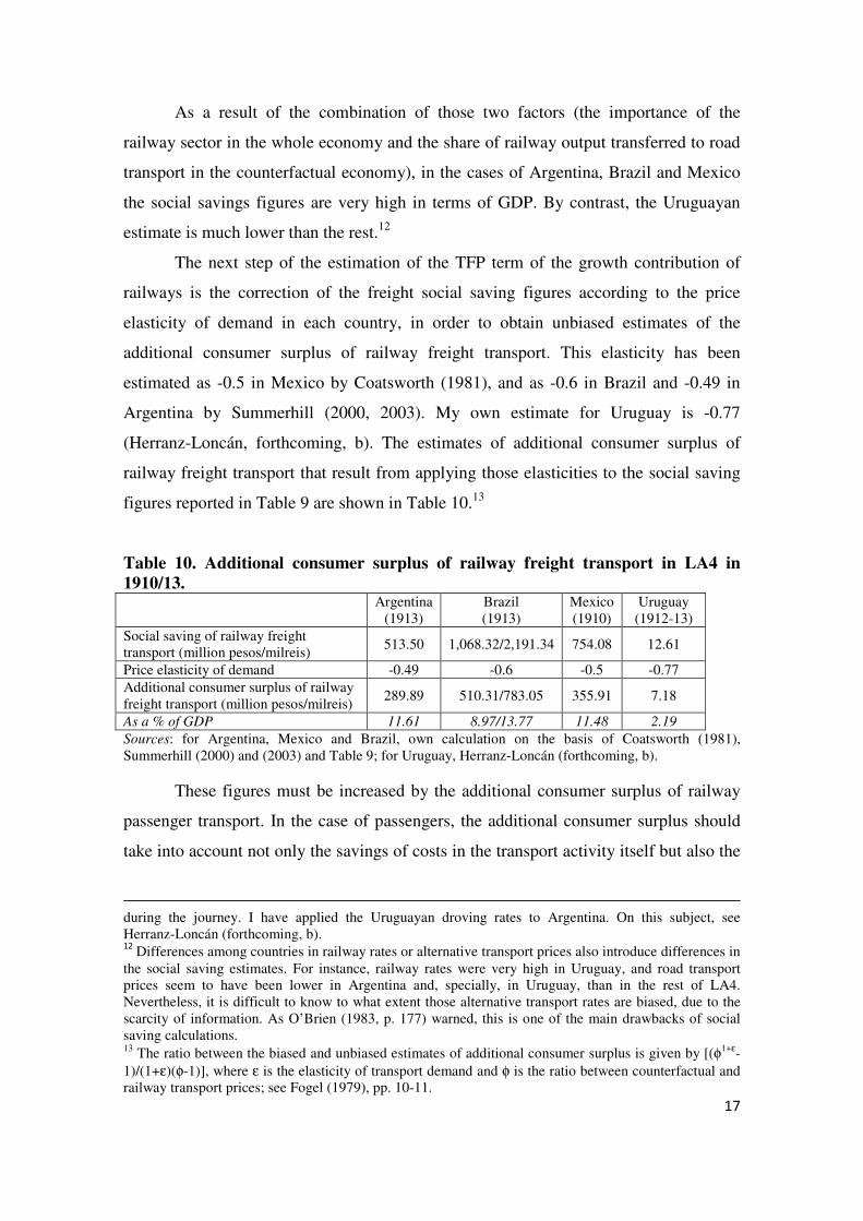
The next step of the estimation of the TFP term of the growth contribution of

railways is the correction of the freight social saving figures according to the price

elasticity of demand in each country, in order to obtain unbiased estimates of the

additional consumer surplus of railway freight transport. This elasticity has been

estimated as -0.5 in Mexico by Coatsworth (1981), and as -0.6 in Brazil and -0.49 in

Argentina by Summerhill (2000, 2003). My own estimate for Uruguay is -0.77

(Herranz-Loncán, forthcoming, b). The estimates of additional consumer surplus of

railway freight transport that result from applying those elasticities to the social saving

figures reported in Table 9 are shown in Table 10.13

Table 10. Additional consumer surplus of railway freight transport in LA4 in

1910/13. Argentina

(1913)

Brazil

(1913)

Mexico

(1910)

Uruguay

(1912-13)

Social saving of railway freight

transport (million pesos/milreis) 513.50 1,068.32/2,191.34 754.08 12.61

Price elasticity of demand -0.49 -0.6 -0.5 -0.77

Additional consumer surplus of railway

freight transport (million pesos/milreis) 289.89 510.31/783.05 355.91 7.18

As a % of GDP 11.61 8.97/13.77 11.48 2.19

Sources: for Argentina, Mexico and Brazil, own calculation on the basis of Coatsworth (1981),

Summerhill (2000) and (2003) and Table 9; for Uruguay, Herranz-Loncán (forthcoming, b).

These figures must be increased by the additional consumer surplus of railway

passenger transport. In the case of passengers, the additional consumer surplus should

take into account not only the savings of costs in the transport activity itself but also the

during the journey. I have applied the Uruguayan droving rates to Argentina. On this subject, see

Herranz-Loncán (forthcoming, b). 12

Differences among countries in railway rates or alternative transport prices also introduce differences in

the social saving estimates. For instance, railway rates were very high in Uruguay, and road transport

prices seem to have been lower in Argentina and, specially, in Uruguay, than in the rest of LA4.

Nevertheless, it is difficult to know to what extent those alternative transport rates are biased, due to the

scarcity of information. As O’Brien (1983, p. 177) warned, this is one of the main drawbacks of social

saving calculations. 13

The ratio between the biased and unbiased estimates of additional consumer surplus is given by [(φ1+ε

-

1)/(1+ε)(φ-1)], where ε is the elasticity of transport demand and φ is the ratio between counterfactual and

railway transport prices; see Fogel (1979), pp. 10-11.

18

time saved by individuals thanks to the replacement of traditional transport means by

railways. This requires estimating the share of additional travelling time that would

have to be deducted from the travellers’ working time in the counterfactual economy, as

well as the railway passengers’ average hourly wage.

As in the case of freight, Coatsworth (1981) and Summerhill (2003) produced

careful estimates of the social savings of railway passenger transport for Mexico and

Brazil, respectively. These were based on the assumption that, in the absence of the

railways, first class passengers would have used stagecoach transport, but second class

passengers would have walked instead. Since my interest is the additional consumer

surplus of passenger transport, and not the mere social savings, here I follow a different

approach. Firstly, I estimate the social savings of railway passenger transport in both

countries considering stagecoach transport as the counterfactual transport system for all

passenger classes. And, secondly, I correct the social saving estimates according to the

price elasticity of demand, but allowing for different elasticities in first and second class

railway transport. More concretely, for first class passengers, I assume the price

elasticity of transport demand to be approximately -1,14

and, for second class

passengers, I consider railway transport as a completely new good. This is equivalent to

assume that the users of second class passenger transport would not have travelled at all

at the price of the most comparable alternative transport system, i.e. stagecoach

transport.15

The result of this strategy is an alternative estimate of the social savings of

passenger railway transport in those two countries, although fully based on the

information provided by those authors.In the cases of Argentina and Uruguay, I have

carried out a similar estimation although, as in the case of freight, I have assumed that,

in the absence of the railways, certain share of the Argentinean and Uruguayan

passenger transport would have been transferred to river navigation. I have estimated

that percentage to be 16.8 percent in Argentina and 16.6 percent in Uruguay.16

As for

the savings in travel time, here I have assumed, as Coatsworth and Summerhill, that the

lowest-income social groups did not use railway transport. Therefore, I value the travel

time of second class travelers at the average hourly wage of industrial workers, and that

of first class travelers at twice that amount. Finally, I also consider, as in the cases of

Mexico and Brazil, that only about half of the time savings were savings in working

14

See, for instance, Boyd and Walton (1972), pp. 247-250, and Metzer (1977), p. 73. 15

See, for instance, Hausman (1994). 16

Those percentages are calculated on the basis of the same assumptions as in the case of freight.

19

time and must therefore be included in the estimation of the additional consumer

surplus.17

The results of the estimation are shown in Table 11.

17

The actual percentages of travel time that were considered working travel time by Coatsworth (1981)

and Summerhill (2003) were 40 and 51.7 percent respectively. I have used the threshold of 50 percent for

the four countries for the sake of homogeneity. However, using those authors’ percentages instead has a

minimum impact on the final results.

20

Table 11. Social savings of railway passenger transport in LA4 in 1910/13. A) First-class passenger transport

Argentina (1913) Brazil (1913) Mexico (1910) Uruguay (1912-13)

a) Railway output (million passenger-km) 1,309.43 605.19 229.91 68.155

b) Railway rate in pesos/milreis per passenger-km (in pounds) 0.015 (0.0031) 0.047 (0.0011) 0.037 (0.0038) 0.019 (0,0041)

c) Railway output (million pesos/milreis) (a x b) 20.21 28.44 8.45 1.30

d) Unit value of working travel time in pesos/milreis per hour (in pounds) 0.452 (0.090) 0.891 (0.0208) 0.356 (0.0367) 0.409 (0.0870)

e) Railway passenger transport average speed (km p. h.) 39.4 39 40 34.4

f) Working travel time by railway (million hours) (50 percent of a at e km p. h.) 16.617 7.759 2.874 0.991

g) Value of the working travel time by railway (million pesos/milreis) (d x f) 7.503 6.913 1.023 0.405

h) Counterfactual water transport output (million passenger-km) 219.52 - - 11.29

i) Counterfactual water transport rate in pesos/milreis per passenger-km (in pounds) 0.0057 (0.0011) - - 0.0048 (0.0010)

j) Counterfactual water transport output (million pesos/milreis) (h x i) 1.251 - - 0.054

k) Water passenger transport average speed (km p. h.) 12 - - 12

l) Working travel time by water transport (million hours) (50 percent of h at k p. h.) 9.147 - - 0.0023

m) Value of the working travel time by water transport (million pesos/milreis) (d x l) 4.130 - - 0.00093

n) Counterfactual road transport output (million passenger-km) 1,089.91 605.19 229.91 56.87

o) Counterfactual road transport rate in pesos/milreis per passenger-km) (in pounds) 0.0246 (0.0049) 0.360 (0.0084) 0.120 (0.0123) 0.0614 (0.0131)

p) Counterfactual road transport output (million pesos/milreis) (n x o) 22.812 217.87 27.609 3.494

q) Road passenger transport average speed (km p. h.) 17.25 13 15 6.5

r) Working travel time by road transport (million hours) (50 percent of n at q km p. h.) 31.592 23.277 7.664 4.374

s) Value of the working travel time by road transport (million pesos/milreis) (d x r) 14.264 20.738 2.728 1.789

t) Savings on transport costs (million pesos/milreis) (j + p – c) 7.855 189.43 19.156 2.248

u) Savings on travel time (million pesos/milreis) (m + s – g) 10.891 13.825 1.705 1.385

v) Total savings (million pesos/milreis) (t + u) 18.746 203.25 20.861 3.633

w) As a percentage of GDP 0.75 3.57 0.67 2.60

21

B) Second-class passenger transport. Argentina (1913) Brazil (1913) Mexico (1910) Uruguay (1912-13)

a) Railway output (million passenger-km) 1,544.28 1,012.00 830.54 47.231

b) Railway rate in pesos/milreis per passenger-km (in pounds) 0.010 (0.0020) 0.027 (0.0006) 0.014 (0.0015) 0.016 (0.0033)

c) Railway output (million pesos/milreis) (a x b) 15.19 26.82 11.90 0.73

d) Unit value of working travel time in pesos/milreis per hour (in pounds) 0.226 (0.0448) 0.445 (0.0104) 0.178 (0.0184) 0.205 (0.0435)

e) Railway passenger transport average speed (km p. h.) 39.4 39 40 34.4

f) Working travel time by railway (million hours) (50 percent of a at e km p. h.) 19.598 12.974 10.382 0.687

g) Value of the working travel time by railway (million pesos/milreis) (d x f) 4.424 5.780 1.848 0.140

h) Counterfactual water transport output (million passenger-km) 258.90 - - 7.82

i) Counterfactual water transport rate in pesos/milreis per passenger-km (in pounds) 0.0057 (0.0011) - - 0.0048 (0.0010)

j) Counterfactual water transport output (million pesos/milreis) (h x i) 1.476 - - 0.038

k) Water passenger transport average speed (km p. h.) 12 - - 12

l) Working travel time by water transport (million hours) (50 percent of h at k p. h.) 10.787 - - 0.0016

m) Value of the working travel time by water transport (million pesos/milreis) (d x l) 2.435 - - 0.00032

n) Counterfactual road transport output (million passenger-km) 1,285.39 1,012.00 830.54 39.41

o) Counterfactual road transport rate in pesos/milreis per passenger-km) (in pounds) 0.0246 (0.0049) 0.360 (0.0084) 0.120 (0.0123) 0.0614 (0.0131)

p) Counterfactual road transport output (million pesos/milreis) (n x o) 31.621 364.32 99.737 2.421

q) Road passenger transport average speed (km p. h.) 17.25 13 15 6.5

r) Working travel time by road transport (million hours) (50 percent of n at q km p. h.) 37.258 38.923 27.685 3.031

s) Value of the working travel time by road transport (million pesos/milreis) (d x r) 8.411 17.339 4.928 0.620

t) Savings on transport costs (million pesos/milreis) (j + p – c) 17.905 337.502 87.842 1.725

u) Savings on travel time (million pesos/milreis) (m + s – g) 6.422 11.559 3.080 0.480

v) Total savings (million pesos/milreis) (t + u) 24.327 349.061 90.922 2.205

w) As a percentage of GDP 0.97 6.14 2.93 1.58

Sources and notes: for Mexico and Brazil, own elaboration based on Coatsworth (1981) and Summerhill (2003); for Argentina and Uruguay, see Herranz-Loncán

(forthcoming, a) and (forthcoming, b).

22

As may be seen in Table 12, when these figures are corrected according to the

elasticity of demand, and under the assumptions described above, the additional

consumer surplus of passenger railway transport becomes much lower, especially in the

case of the second class, as a result of the assumption that this category of passenger

transport was a completely new good. The resulting total additional consumer surplus

for passenger transport is, therefore, much smaller than in the case of freight, which is

consistent with the low importance that passenger transport had, according to

Coatsworth (1981) and Summerhill (2003), in the direct benefits that Mexico and Brazil

received from the railways. The only exception to that rule is Uruguay, due to the low

size of the social saving of freight transport in that country.

Table 12. Additional consumer surplus of railway passenger transport in LA4

(corrected by the elasticity of demand) Argentina

(1913)

Brazil

(1913)

Mexico

(1910)

Uruguay

(1912-13)

a) First-class (million pesos/milreis) 16.65 68.55 12.25 2.31

b) Second-class (million pesos/milreis) 0.44 4.01 1.31 0.05

Total (a+b) 17.09 72.57 13.56 2.36

As a % of GDP 0.68 1.28 0.44 1.69

Sources: see text and Table 11.

The scarcity of adequate information prevents from including in the additional

consumer surplus estimates other sorts of freight transport (essentially high-speed

freight), which accounted for a non-negligible share of railway revenues.18

Their

absence would introduce certain downward bias in the additional consumer surplus

figures. This bias, however, is probably small. Since, as in the case of second class

passenger transport, most of that traffic should be considered as a completely new

commodity, its contribution to the additional consumer surplus may be expected to be

rather low.

Finally, in order to obtain a complete measure of the real income gain provided

by the railways in each country, the estimates of the additional consumer surplus of

freight and passenger transport should be corrected for the potential presence of

supernormal profits in the railway system. Supernormal profits should be calculated as

the difference between gross revenues and total expenditure, including capital costs.

18

For instance, this kind of traffic accounted for 11.8 percent of the total revenues of the Brazilian

railway companies in 1913 (percentage estimated from Summerhill, 2003), for 4.8 percent in the case of

Argentina (estimated from Dirección General de Ferrocarriles, Estadística de los ferrocarriles en

explotación, 1913), and 4.9 in Uruguay (see Herranz-Loncán, forthcoming, b).

23

The latter, in turn, may be calculated as a percentage of the value of the stock of railway

capital, which should include both the amortisation rates and the opportunity cost of

capital. This calculation, however, is far from easy, due to the accounting procedures

that were followed at the time. On the one hand, operating costs often included some

replacement and new investment expenditures, which were not, therefore, incorporated

to the capital account. On the other hand, railway capital was rarely depreciated, leading

to an overstatement of the capital stock figures.19

In addition, in those countries, such as

Argentina or Brazil, where railway subsidies mainly consisted on guaranteed returns

upon investment, capital figures were often artificially inflated by the companies.20 In

this context, it is very difficult to obtain an accurate estimate of supernormal profits.

Therefore, here I just compare the difference between the net returns of each system and

the opportunity cost of capital, approached through yields to government bonds, in

order to have a preliminary idea of their potential size.

By 1912-13, railway net operating returns were around 4 percent of total

investment in Argentina, 3.6 percent in Brazil and 4 percent in Uruguay.21

Given that

the yields to government bonds were 4.88 percent in Argentina and 4.97 percent in

Brazil at the time (Flandreau and Zumer, 2004), it seems likely that supernormal profits

were actually negative in those railway systems, since net revenues would not have been

sufficient to cover capital costs. However, those negative returns would be relatively

small, specially compared with the additional consumer surplus of railway transport.

For instance, in the case of Argentina and Brazil, if I take the yields on bonds as a

proxy of the opportunity cost of capital and ignore amortization needs, that correction

would amount to just 3-4.5 percent of the additional consumer surplus. Therefore, given

the uncertainty on the real value of investment in those railway systems, I have decided

to exclude this correction from the final figures.

19

See Summerhill (2003), p. 169. 20

This is the typical Averch-Johnson effect; see Averch and Johnson (1962). In the case of the

Ferrocarril Central Argentino, López del Amo (1989), pp. 240-241, estimates that the company’s

accounts exaggerated investment figures by 57 percent between 1908 and 1930. 21

Railway net returns come, in the case of Argentina, from Dirección General de Ferrocarriles,

Estadística de los ferrocarriles en explotación (1913); in the case of Brazil, from Summerhill (2003); and,

in the case of Uruguay, from Herranz-Loncán (forthcoming, b). In the case of Mexico, there are no

available estimates of the total capital invested in the railway network and, therefore, it is not possible to

calculate an average rate of return; see Ortiz Hernán (1996), p. 28. However, if the net revenues of the

system by 1910 are combined with the estimate of 1,130 million pesos of foreign investment in Connolly

(1997), p. 83, the resulting percentage is less than 3 percent. Therefore, the situation would not be very

different to the other three countries.

24

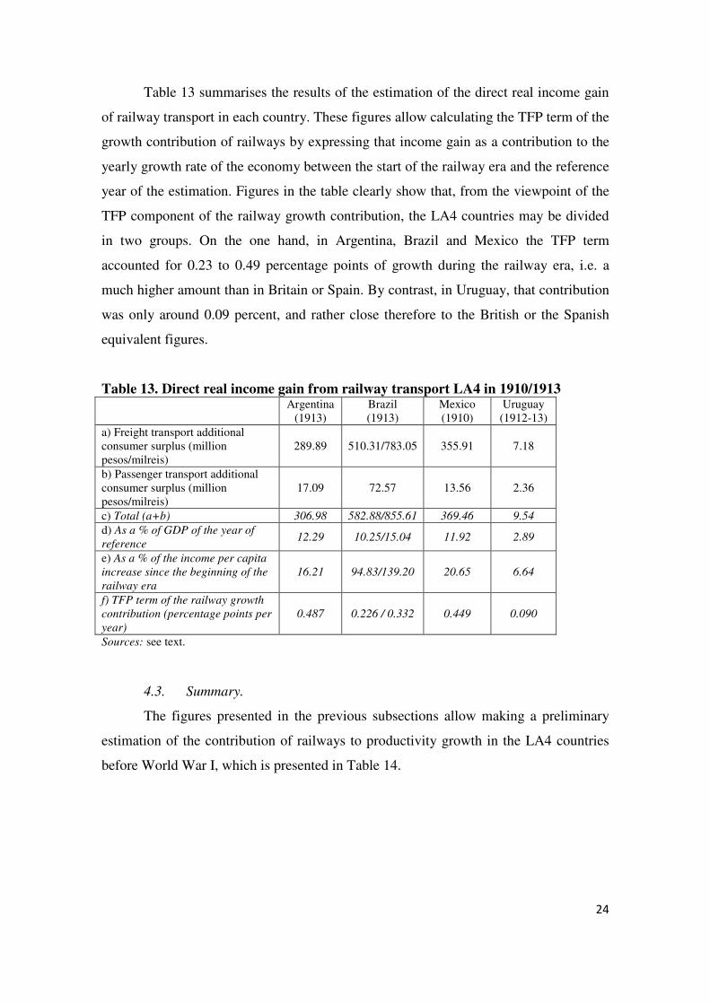
Table 13 summarises the results of the estimation of the direct real income gain

of railway transport in each country. These figures allow calculating the TFP term of the

growth contribution of railways by expressing that income gain as a contribution to the

yearly growth rate of the economy between the start of the railway era and the reference

year of the estimation. Figures in the table clearly show that, from the viewpoint of the

TFP component of the railway growth contribution, the LA4 countries may be divided

in two groups. On the one hand, in Argentina, Brazil and Mexico the TFP term

accounted for 0.23 to 0.49 percentage points of growth during the railway era, i.e. a

much higher amount than in Britain or Spain. By contrast, in Uruguay, that contribution

was only around 0.09 percent, and rather close therefore to the British or the Spanish

equivalent figures.

Table 13. Direct real income gain from railway transport LA4 in 1910/1913

Argentina

(1913)

Brazil

(1913)

Mexico

(1910)

Uruguay

(1912-13)

a) Freight transport additional

consumer surplus (million

pesos/milreis)

289.89 510.31/783.05 355.91 7.18

b) Passenger transport additional

consumer surplus (million

pesos/milreis)

17.09 72.57 13.56 2.36

c) Total (a+b) 306.98 582.88/855.61 369.46 9.54

d) As a % of GDP of the year of

reference 12.29 10.25/15.04 11.92 2.89

e) As a % of the income per capita

increase since the beginning of the

railway era

16.21 94.83/139.20 20.65 6.64

f) TFP term of the railway growth

contribution (percentage points per

year)

0.487 0.226 / 0.332 0.449 0.090

Sources: see text.

4.3. Summary.

The figures presented in the previous subsections allow making a preliminary

estimation of the contribution of railways to productivity growth in the LA4 countries

before World War I, which is presented in Table 14.

25

Table 14. The contribution of railways to productivity growth in LA4 before 1914

(percentage points per year) Argentina

(1865-1913)

Brazil

(1864-1913)

Mexico

(1873-1910)

Uruguay

(1874-1913)

a) Railway capital stock per capita growth 6.36 6.25 8.61 3.91

b) Railway profits share in national income 1.81 0.81 0.91 0.71

c) Railway capital contribution (a x b) 0.115 0.051 0.079 0.028

d) TFP contribution 0.487 0.226 / 0.332 0.449 0.090

e) TFP Spillovers na na na na

f) Total railway contribution (c+d) 0.602 0.277/0.383 0.528 0.118

g) GDP per capita growth 3.00 0.24 2.17 1.35

h) Railway contribution as % of GDP

growth (f/g) 20.04 116.1/160.5 24.27 8.71

na: not available.

Sources: GDP per capita growth rates are calculated, in the case of Argentina, from the estimates by Della

Paolera, Taylor and Bózzoli (2003) (I assume a 0.8 percent yearly growth rate before 1875, following

Prados de la Escosura, 2010); in the case of Brazil, from Goldsmith (1986) and, since 1900, Haddad

(1978); in the case of Mexico, from the Maddison’s database; and, in the case of Uruguay, from Bértola

(1998). For other magnitudes, see text.

Figures in Table 14 clearly confirm the exceptional character of Uruguay within

the LA4 sample. Despite the substantial effort made to endow the Uruguayan economy

with one of the densest networks of the continent, the direct contribution of the railways

to economic growth was much lower than in the rest of LA4 and also lower than in

Britain and Spain, both in absolute and relative terms. Uruguay provides therefore an

interesting counterexample of a Latin American country in which the construction of

railways during the first globalization constituted a relative failure. This result is

partially associated to the low level of the capital term, due to the relative slowdown of

Uruguayan railway construction since the 1890s. However, the main reason for that

outcome is the low size of railway output in Uruguay by 1913. As is indicated in

Herranz-Loncán (forthcoming, b), there are several potential explanations for the

underdevelopment of the Uruguayan railway sector: alternative water transport was

available for many routes, the specialisation of the country in livestock production did

not generate much transport output per km2, and the small scale of the country increased

the share of short distance journeys over total transport, reducing therefore the

competitiveness of the railways over traditional overland transport means. In other

words, and opposite to what happened in the other LA4 countries, the geography of

Uruguay did not provide an adequate context for achieving all the potential benefits of

the new technology.

By contrast, the size of the direct growth contribution of railways in Argentina,

Brazil and Mexico is, by all means, impressive. In absolute terms, the railways provided

26

between 0.3 and 0.6 percentage points of growth per year in each of those three

countries, i.e. between two and four times the equivalent figure in Britain or Spain.

Such an advantage was, once more, mainly associated to the TFP effect. The capital

term, by contrast, only made a significant difference in Argentina, due to the large share

that railways net revenues accounted for within national income by 1913.

The high level of the TFP terms in those countries had several origins. In the

cases of Brazil and Mexico, its most important explanatory factor was the absence of

alternatives to road transport in a counterfactual economy without railways. This

generated a huge difference between the railway rates and the alternative transport

costs, with a large effect in the estimated direct income gains. In the case of Argentina,

the size of the TFP term may also be explained, once more, by the large share that

railways accounted for in the economy, as well as by the high efficiency of the

Argentinean railway system, which applied the lowest rates to freight transport in the

LA4 sample. All those reasons together help to explain that Argentina, Mexico and

Brazil obtained huge absolute benefits from railway construction during the first

globalization period.

The last row of Table 14 reports the growth contribution of railways as a

percentage of the actual rate of growth of income per capita in each country. As has

been indicated, Uruguay also stands out by the low level of the growth contribution of

their railways in relative terms: just 8.7 percent of the growth of income per capital, i.e.

a much lower percentage than in Britain or Spain. By contrast, in Argentina and Mexico

the railways were directly responsible for 20 to 25 of the growth of income per capita

between the start of the railway era and 1910/1913. Those percentages are quite

impressive for a single sector, and significantly higher than the Spanish or British

equivalent figures. Moreover, it is necessary to recall that those percentages exclude the

indirect effects of railways, due to the difficulty to quantify them. In this regard, it is

plausible to assume that the TFP spillovers of the railways were more important in Latin

America than in Europe, because, in the former, they allowed the exploitation of the

natural resources of a large share of the territory, which would have remained idle

without them (Summerhill, 2003, p. 78). This would be especially relevant in the

Argentinean case, since the main export during the period under study, i.e. grain, was

absolutely dependent on railway transport (Cortés Conde, 1979; Lewis, 1983, pp. 219-

220; López, 2007, pp. 46-51). As long as economic growth was led by exports, the

27

indirect impact of railways during the period might have been almost as important as

the direct effect, and the advantage of Argentina over Spain or Britain would be even

larger than the figures in Table 14 explain.

In this context, Brazil deserves a special comment. Although the contribution of

railways was lower in that country than in Argentina and Mexico in terms of percentage

points of growth, that contribution was actually higher than the total growth of the

stagnated Brazilian economy during the decades prior to 1914. This might be taken as a

confirmation of Summerhill’s statement that: “the railroad conferred on Brazil benefits

that probably exceeded, by far, those stemming from the other major changes in

economic organization in this period” (Summerhill, 2003, p. 96). However, the ratio is

too high to be believed, and this anomaly raises some questions on the accuracy of the

analysis that has been carried out in this paper. In this regard, it is possible, of course,

that the available estimates of Brazilian income per capita of the late nineteenth and

early twentieth century underestimate the actual growth of the Brazilian economy, since

there is still a large margin of improvement of the long term economic history series of

the main Latin American economies. However, the ratios reported in Table 14 may also

reflect the fact that, in some cases, the country level may not be the most adequate scale

to carry out analyses of the growth impact of the railways. During the period under

analysis, the Brazilian economy constituted a huge and hardly integrated economic

space. The absence of integration was also visible in the railways, which, opposite to

what happened in Argentina, Mexico or Uruguay, did not constitute a national network,

but were divided in several sub-systems, only partially connected through coastal

navigation. In this context, the stagnation of 1865-1913, as has been suggested by the

historiography, was compatible with considerable changes in the economic geography

of the country, with some regions growing at high rates and other areas sinking into a

deep crisis. As might be expected, the most important of those systems were established

in the more dynamic areas (Sao Paulo and Rio de Janeiro), whereas the rest of the

country only had some scattered lines that did not constitute intertwined networks. It is

arguable to what extent, in such an economy, measuring the impact of the railways at

the national level is meaningful. Probably, carrying out the analysis at the regional level

28

would provide indicators much more relevant for the understanding of the role of the

railways in each economic space.22

5. Concluding remarks

Railways constituted one of the most important technological breakthroughs of

the nineteenth century, leading to a substantial upward shift in national economies’

production functions worldwide. In the case of Latin America, historians have often

highlighted the importance of railways for economic growth during the first

globalisation boom, and the social saving literature has given empirical support to the

hypothesis that those Latin American countries that invested heavily in railways

obtained higher benefits from them than the more developed economies of Europe or

North America. In this context, this paper has provided estimates of the direct

contribution of railways to productivity growth in Argentina, Brazil, Mexico and

Uruguay, which were among those Latin American economies that built relatively dense

networks during the first globalisation boom. The results of the estimation indicate,

firstly, that the contribution of railways to growth varied substantially across Latin

American countries. More precisely, in the case of Uruguay, the growth impact of

railways was very low, lower actually than in some European countries, such as Britain

and Spain. This unexpected result may be explained by the features of the Uruguayan

geography and economic structure, and provides a clear counterexample to the

hypothesis that railways had higher benefits in Latin America than in the core

industrialised countries.

By contrast, in the other three countries under study (Argentina, Mexico and

Brazil) the railways provided huge direct benefits that amounted, in the first two cases,

to between one fifth and one quarter of the total income per capita growth of the period

under analysis. Besides, those ratios should be increased by the indirect spillovers

coming from the railway system. Specially in the case of new settlement countries, such

as Argentina, these may be expected to have been also very high, compared with those

received from the railways by those economies that were relatively well developed and

integrated at the advent of the railways (such as the UK). Finally, the case of Brazil

merits a special reference, since the outcome of the analysis carried out in this paper

22

For instance, if the analysis of the impact of railways is applied to the economic area organised around

Sao Paulo and Rio de Janeiro it would probably provide a lower ratio in row h and, in the case of the

North-East regions, it would probably produce a much lower level of the percentage in row f.

29

would indicate that the direct contribution of railways to growth would be higher than

the whole income per capita growth of the Brazilian economy before 1914. Keeping in

mind the possible biases associated to the lack of precision of the available income

figures, this unexpected result would also suggest that the national level may not be the

most adequate scale to analyse the economic impact of network infrastructure in the

case of large, geographically unequal and insufficiently integrated developing

economies.

6. References

Averch, H. and Johnson, L. L. (1962), “Behavior of the Firm Under Regulatory

Constraint”, American Economic Review, 52, 5, pp. 1052-1069.

Bertino, M. and Tajam, H. (1999), El PBI de Uruguay, 1900-1955, Montevideo,

Universidad de la República, Instituto de Economía.

Bértola, L. (1998), El PBI de Uruguay 1870-1936 y otras estimaciones, Montevideo,

Universidad de la República, Facultad de Ciencias Sociales.

Boyd, J. H. and Walton, G. M. (1972), “The Social Savings from Nineteenth-Century

Rail Passenger Services”, Explorations in Economic History, 9, 3, pp. 233-254.

Caron, F. (1983), “France”, in O’Brien, P. (ed.), Railways and the Economic Growth of

Western Europe, London, McMillan, pp. 28-48.

Coatsworth, J. H. (1979), “Indispensable Railroads in a Backward Economy: The Case

of Mexico”, Journal of Economic History, 39, 4, pp. 939-960.

Coatsworth, J. H. (1981), Growth against Development: The Economic Impact of

Railroads in Porfirian Mexico, DeKalb, Northern Illinois University Press.

Connolly, P. (1997), El contratista de don Porfirio. Obras públicas, deuda y desarrollo

regional, Zamora, Colegio de Michoacán.

Cortés Conde, Roberto (1979), El progreso argentino, 1880-1914, Buenos Aires,

Editorial Sudamericana.

Crafts, N. F. R. (2004a), “Social Savings as a Measure of the Contribution of a New

Technology to Economic Growth”, LSE, Department of Economic History

Working Paper 06/04.

Crafts, N. F. R. (2004b), “Steam as a General Purpose Technology: A Growth

Accounting Perspective”, Economic Journal, 114, pp. 338-351.

Crafts, N. F. R. (2010), “The Contribution of New Technology to Economic Growth:

Lessons from Economic History”, Revista de Historia Económica-Journal of

Iberian and Latin American Economic History, 28 (3), pp. 409-440.

Della Paolera, G.; Taylor, A. M. and Bózzoli, C. G. (2003), “Historical Statistics”, in

Della Paolera, G. and Taylor, A. M. (eds.), A New Economic History of

Argentina, Cambridge, Cambridge University Press, pp. 376-385.

Dobado, R. and Marrero, G. A. (2005), “Corn Market Integration in Porfirian Mexico”,

Journal of Economic History, 65, 1, pp. 103-128.

Ferreres, O. (2005), Dos siglos de economía argentina. Historia argentina en cifras,

Fundación Norte y Sur.

Fishlow, A. (1965), American Railroads and the Transformation of the Ante-bellum

Economy, Cambridge (MA), Harvard University Press.

30

Flandreau, M. and Zumer, F. (2004), The Making of Global Finance, 1880-1913, Paris,

OECD.

Fogel, R. W. (1964), Railroads and American Economic Growth: Essays in

Econometric History, Baltimore.

Fogel, R. W. (1979), “Notes on the Social Saving Controversy,”, Journal of Economic

History, 39, 1, pp. 1-54.

Goldsmith, R. (1986), Brasil 1850-1984: desenvolvimento financeiro sob um século de

inflação, São Paulo, Harper & Row do Brasil.

Grunstein Dickter, A. (1996), “¿Competencia o monopolio? Regulación y desarrollo

ferrocarrilero en México, 1885-1911”, in Kuntz Ficker, S. and Riguzzi, P. (eds.),

Ferrocarriles y vida económica en México (1850-1950). Del surgimiento tardío

al decaimiento precoz, México, El Colegio Mexiquense, pp. 167-221.

Haddad, C. (1978), Crescimento do produto real no Brasil, 1900-1947, Rio de Janeiro,

FGV.

Hausman, J. A. (1994), “Valuation of New Goods under Perfect and Imperfect

Competition”, NBER Working Paper 4970.

Hawke, G. R. (1970), Railways and Economic Growth in England and Wales, Oxford,

Clarendon Press.

Herranz-Loncán, A. (2006), “Railroad Impact in Backward Economies: Spain, 1850-

1913”, Journal of Economic History, 66, 4, pp. 853-881.

Herranz-Loncán, A. (2008), Infraestructuras y crecimiento económico en España,

1850-1935, Madrid, Fundación de los Ferrocarriles Españoles.

Herranz-Loncán, A. (forthcoming, a), “El impacto directo del ferrocarril sobre el

crecimiento económico argentino durante la Primera Globalización”, Revista de

la Asociación Uruguaya de Historia Económica.

Herranz-Loncán, A. (forthcoming, b), “The Role of Railways in Export-Led Growth:

the Case of Uruguay, 1870-1913”, Economic History of Developing Regions.

Jara-Díaz, S. R. (1986), “On the Relation Between Users’ Benefits and the Economic

Effects of Transportation Activities”, Journal of Regional Science, 26, 2, pp.

379-391.

Kuntz Ficker, S. (1995), “Mercado interno y vinculación con el exterior: el papel de los

ferrocarriles en la economía del porfiriato”, Historia Mexicana, XLV, 1, pp. 39-

66.

Kuntz Ficker, S. (1999), “Los ferrocarriles y la formación del espacio económico en

México, 1880-1910”, in Kuntz Ficker, S. and Connolly, P. (coord.),

Ferrocarriles y Obras Públicas, México, Instituto Mora, pp. 105-137.

Leunig, T. (2010), “Social Savings”, Journal of Economic Surveys, 24, 5, pp. 775-800.

Lewis, C. (1983), British Railways in Argentina, 1857-1914, London, Institute of Latin

American Studies.

López, Mario Justo (2007), “La combinación de la acción nacional y provincial y la

suma del capital privado y público en la construcción de las primeras líneas

ferroviarias, 1857-1886”, in López, Mario Justo and Waddell, Jorge E. (comps.),

Nueva historia del ferrocarril en la Argentina. 150 años de política ferroviaria,

Buenos Aires, Lumiere.

López del Amo, F. (1989), Ferrocarril, ideología y política ferroviaria en el proyecto

liberal argentino (1852-1916), University of Barcelona, PhD Thesis.

Maddison, A. (2001), The World Economy: A Millennial Perspective, Paris, OECD.

31

Metzer, J. (1977), Some Economic Aspects of Railroad Development in Tsarist Russia,

New York, Arno Press.

Metzer, J. (1984), “Railroads and the Efficiency of Internal Markets: Some Conceptual

and Practical Considerations”, Economic Development and Cultural Change, 33,

1, pp. 61-70.

Mitchell, B.R. (2003), International Historical Statistics: The Americas, 1750-2000,

Houndmills, Palgrave.

O’Brien, P., (1983): “Transport and Economic Development in Europe, 1789-1914”, in

O’Brien, P. (ed.), Railways and the Economic Growth of Western Europe,

London, McMillan, pp. 1-27.

Oliner, S. D. and Sichel, D. E. (2002), “Information Technology and Productivity:

Where Are We Now and Where Are We Going”, Federal Reserve Bank of

Atlanta Economic Review, 87, 3, pp. 15-44.

Ortiz Hernán, S. (1996), “Introducción”, in Kuntz Ficker, S. and Riguzzi, P. (eds.),

Ferrocarriles y vida económica en México (1850-1950). Del surgimiento tardío

al decaimiento precoz, México, El Colegio Mexiquense, pp. 15-30.

Prados de la Escosura, Leandro (2009), “Lost Decades? Economic Performance in Post-

Independence Latin America”, Journal of Latin American Studies, 41, pp. 279-

307.

Ramírez, M. T. (2001), “Los ferrocarriles y su impacto sobre la economía colombiana”,

Revista de Historia Económica, 19, 1, pp. 81-122.

Summerhill, W. (2000), “Profit and Productivity on Argentine Railroads, 1857-1913”,

Los Angeles, UCLA, Department of History, UCLA (mimeo).

Summerhill, W. (2003), Order Against Progress. Government, Foreign Investment, and

Railroads in Brazil, 1854-1913, Stanford, Stanford University Press.

Summerhill, William R. (2006), “The Development of Infrastructure”, in Bulmer-

Thomas, Victor; Coatsworth, John and Cortés Conde, Roberto (eds.), The

Cambridge Economic History of Latin America. Vol. 2: The Long Twentieth

Century, Cambridge, Cambridge University Press, pp. 293-326.

Vázquez-Presedo, V. (1971), Estadísticas históricas argentinas (comparadas). Primera

parte 1875-1914, Buenos Aires, Ediciones Macchi.