arX

iv:a

stro

-ph/

0406

095v

2 1

8 A

ug 2

004

The Cosmic Energy Inventory

Masataka FukugitaInstitute for Advanced Study, Princeton, NJ 08540 USA

and

Institute for Cosmic Ray Research, University of Tokyo,

Kashiwa 277-8582, Japan

P. J. E. PeeblesJoseph Henry Laboratories, Princeton University,

Princeton, NJ 08544 USA

ABSTRACT

We present an inventory of the cosmic mean densities of energy associated with all the knownstates of matter and radiation at the present epoch. The observational and theoretical basesfor the inventory have become rich enough to allow estimates with observational support for thedensities of energy in some 40 forms. The result is a global portrait of the effects of the physicalprocesses of cosmic evolution.

Subject headings: cosmology

1. Introduction

There is now a substantial observational basisfor estimates of the cosmic mean densities of allthe known and more significant forms of matterand energy in the present-day universe. The com-pilation of the energy inventory offers an overviewof the integrated effects of the energy transfers in-volved in all the physical processes of cosmic evo-lution operating on scales ranging from the Hub-ble length to black holes and atomic nuclei. Thecompilation also offers a way to assess how wellwe understand the physics of cosmic evolution, bythe degree of consistency among related entries.Very significant observational advances, particu-larly from large-scale surveys including the Two

Degree Field Galaxy Redshift Survey (2dF: Collesset al. 2001), the Sloan Digital Sky Survey (SDSS:York et al. 2000; Abazajian et al. 2003), theTwo Micron All-Sky Survey (2MASS: Huchra etal. 2003), the HI Parkes All Sky Survey (HIPASS:Zwaan et al. 2003), and the Wilkinson Microwave

Anisotropy Probe (WMAP: Bennett et al. 2003a),make it timely to compile what is known about

the entire energy inventory.

We present here our choices for the categoriesand estimates of the entries in the inventory. Manyof the arguments in this exercise are updated ver-sions of what is in the literature. Some argumentsare new, as is the adoption of a single universalunit — the density parameter — that makes com-parisons across a broad variety of forms of energyimmediate, but the central new development isthat the considerable range of consistency checksdemonstrates that many of the entries in the in-ventory are meaningful and believable.

People have been making inventories for a longtime. The medieval Domesday Book (1086-7) gaveKing William a picture of the wealth and organi-zation of the kingdom (and it gives us fascinat-ing insight into a society). The present-day cos-mic energy inventory similarly gives us a pictureof the amount and organization of the materialcontents of the universe. It also offers us a wayto assess the reliability of our picture, throughchecks of consistency. A early example of the lat-ter point is de Sitter’s (1917) discussion of Ein-

1

stein’s (1917) static homogeneous universe. Underthe assumption that observations can reach a fairsample of the universe, one can seek constraintson the cosmic mean mass density and space cur-vature and test the predicted relation between thetwo. Hubble’s (1929) redshift-distance relation ledto a revision of the predicted relation between themass density and space curvature, and his useof redshifts to convert galaxy counts into num-ber densities greatly improved the estimate of themean mass density (Hubble 1934).1 One may alsoconsider the relations among the mean luminos-ity density of the galaxies, the production of theheavy elements, and the surface brightness of thenight sky (Partridge & Peebles 1967; Peebles &Partridge 1967); the relation between galaxy col-ors, the initial mass function, and the star forma-tion history (Searle, Sargent, & Bagnuolo 1973);the relation between the last two sets of consid-erations (Tinsley 1973); the relation between thelight element abundances and the baryon massdensity (Gott et al. 1974); and the relation be-tween the luminosity density of the quasars andthe mean mass density in quasars and their rem-nants (So ltan 1982). Basu and Lynden-Bell (1990)show how one can analyze what is learned fromthis rich set of considerations in terms of an en-tropy inventory. We have chosen instead to basethis discussion on an energy inventory.

Our inventory includes the mass densities in thevarious states of baryons. This is an updated ver-sion of the baryon budget of Fukugita, Hogan &Peebles (1998; FHP). Most entries in this part ofthe inventory have not changed much in the pasthalf decade, while substantial advances in the ob-servational constraints have considerably reducedthe uncertainties. It appears that most of thebaryonic components are observationally well con-strained, apart from the largest entry, for warmplasma, which still is driven by the need to bal-ance the budget rather than more directly by theobservations.

The largest entries, for dark matter and the cos-mological constant, or dark energy, are well con-strained within a cosmological theory that is rea-

1Hubble’s (1936) estimate based on galaxy masses derivedfrom the velocity dispersion in the Virgo Cluster, whichtakes account of what is now termed nonbaryonic dark mat-ter, translates to density parameter Ωm ∼ 0.1, impressivelyclose to the modern value.

sonably well tested, but the physical natures ofthese entries remain quite hypothetical. We un-derstand the physical natures of magnetic fieldsand cosmic rays, but the theories of the evolutionof these components, and the estimates of theircontributions to the present energy inventory, arequite uncertain. The situation for most of theother entries tends to be between these extremes:the physical natures of the entries are adequatelycharacterized, for the most part, and our estimatesof their energy densities, while generally not veryprecise, seem to be meaningfully constrained bythe observations.

Several cautionary remarks are in order. First,some types of energy are not readily expressed assums of simple components; we must adopt con-ventions. Second, there is no arrangement of cate-gories that offers a uniquely natural place for eachcomponent; we must again adopt conventions.Perhaps further advances in the understanding ofcosmic evolution will lead to a more logically or-dered inventory. Third, it is arguably artificialto represent binding energies as very small nega-tive density parameters. The advantage is that itsimplifies comparisons across the entire inventory.Fourth, the amount of space we devote is in accordwith the importance of the issues of physics andastronomy, not with the value of the energy. Forinstance, the major components in the inventoryare dark energy and dark matter, but they arephysically simple in that their work is only grav-itational, so our discussion is rather short. Dissi-pative energies are small in absolute values, buttheir physical significance is large, and our dis-cussions are on occasion rather lengthy. Finally,it is a task for future work to make some of ourestimates more accurate by using data and com-putations that exist but are difficult to assemble.We mention the main examples in §3.

The inventory, which is presented in Table 1,is arranged by categories and components withincategories. The explanations of conventions andsources for each entry are presented in §2, in sub-sections with numbers keyed to the category num-bers in the first column of the table. Our dis-cussion of checks of the entries is not so simplyordered, because the checks depend on relationsamong considerations of entries scattered throughthe table. A guide to the considerable variety ofchecks detailed in §2 is presented in §3.

2

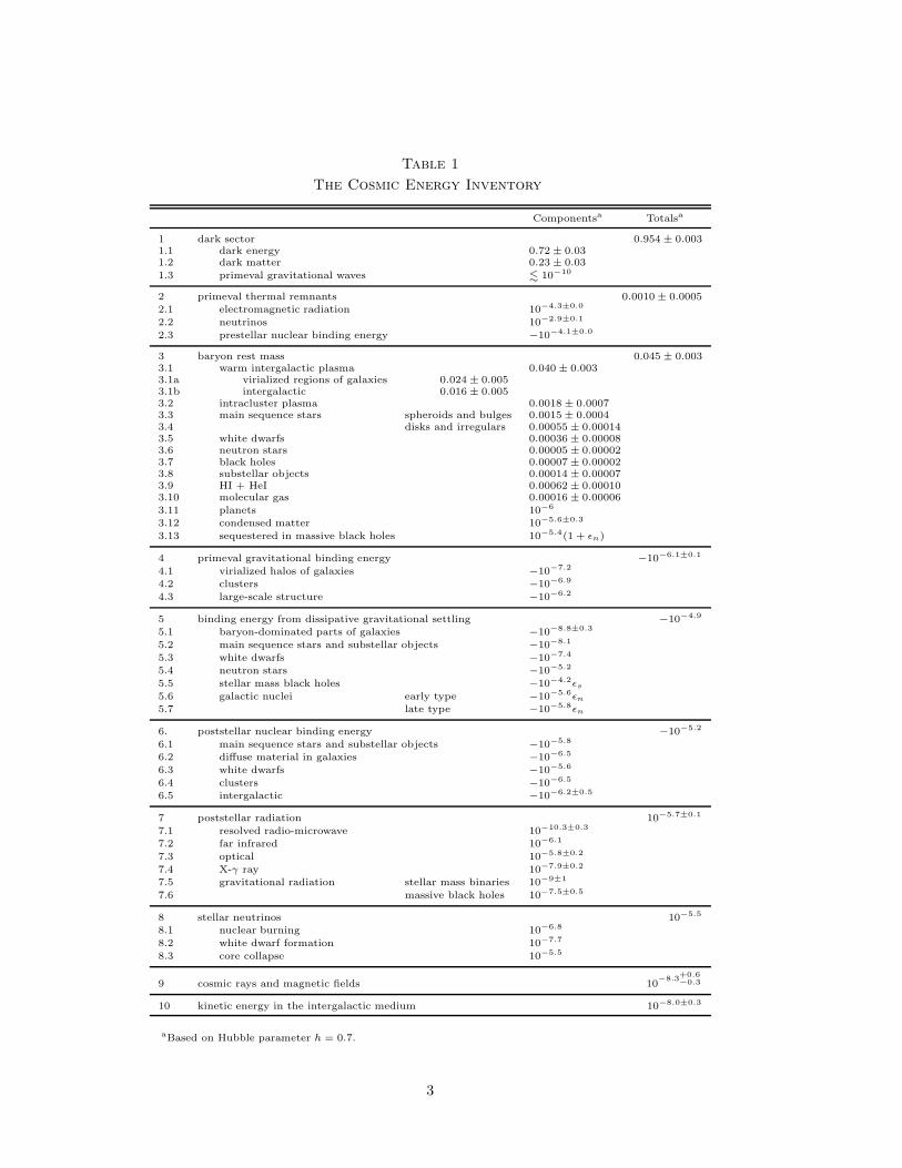
Table 1

The Cosmic Energy Inventory

Componentsa Totalsa

1 dark sector 0.954 ± 0.0031.1 dark energy 0.72 ± 0.031.2 dark matter 0.23 ± 0.03

1.3 primeval gravitational waves . 10−10

2 primeval thermal remnants 0.0010 ± 0.00052.1 electromagnetic radiation 10−4.3±0.0

2.2 neutrinos 10−2.9±0.1

2.3 prestellar nuclear binding energy −10−4.1±0.0

3 baryon rest mass 0.045 ± 0.0033.1 warm intergalactic plasma 0.040 ± 0.0033.1a virialized regions of galaxies 0.024 ± 0.0053.1b intergalactic 0.016 ± 0.0053.2 intracluster plasma 0.0018 ± 0.00073.3 main sequence stars spheroids and bulges 0.0015 ± 0.00043.4 disks and irregulars 0.00055 ± 0.000143.5 white dwarfs 0.00036 ± 0.000083.6 neutron stars 0.00005 ± 0.000023.7 black holes 0.00007 ± 0.000023.8 substellar objects 0.00014 ± 0.000073.9 HI + HeI 0.00062 ± 0.000103.10 molecular gas 0.00016 ± 0.00006

3.11 planets 10−6

3.12 condensed matter 10−5.6±0.3

3.13 sequestered in massive black holes 10−5.4(1 + ǫn)

4 primeval gravitational binding energy −10−6.1±0.1

4.1 virialized halos of galaxies −10−7.2

4.2 clusters −10−6.9

4.3 large-scale structure −10−6.2

5 binding energy from dissipative gravitational settling −10−4.9

5.1 baryon-dominated parts of galaxies −10−8.8±0.3

5.2 main sequence stars and substellar objects −10−8.1

5.3 white dwarfs −10−7.4

5.4 neutron stars −10−5.2

5.5 stellar mass black holes −10−4.2ǫs

5.6 galactic nuclei early type −10−5.6ǫn

5.7 late type −10−5.8ǫn

6. poststellar nuclear binding energy −10−5.2

6.1 main sequence stars and substellar objects −10−5.8

6.2 diffuse material in galaxies −10−6.5

6.3 white dwarfs −10−5.6

6.4 clusters −10−6.5

6.5 intergalactic −10−6.2±0.5

7 poststellar radiation 10−5.7±0.1

7.1 resolved radio-microwave 10−10.3±0.3

7.2 far infrared 10−6.1

7.3 optical 10−5.8±0.2

7.4 X-γ ray 10−7.9±0.2

7.5 gravitational radiation stellar mass binaries 10−9±1

7.6 massive black holes 10−7.5±0.5

8 stellar neutrinos 10−5.5

8.1 nuclear burning 10−6.8

8.2 white dwarf formation 10−7.7

8.3 core collapse 10−5.5

9 cosmic rays and magnetic fields 10−8.3

+0.6−0.3

10 kinetic energy in the intergalactic medium 10−8.0±0.3

aBased on Hubble parameter h = 0.7.

3

2. The Energy Inventory

The inventory in Table 1 assumes the now stan-dard relativistic Friedmann-Lemaıtre ΛCDM cos-mology, in which space sections at fixed worldtime have negligibly small mean curvature,2 Ein-stein’s cosmological term, Λ, is independent oftime and position, the dark matter is an initiallycold noninteracting gas, and primeval departuresfrom homogeneity are adiabatic, Gaussian, andscale-invariant. Physics in the dark sector is notwell constrained: Λ might be replaced with a dy-namical component,3 as in the models for darkenergy now under discussion, the physics of thedark matter may prove to be more complicatedthan that of a free collisionless gas, and the initialconditions may not be adequately approximatedby the present standard cosmology. If such com-plications were present we expect their effects onentries that are sensitive to the cosmological modelwould be slight, however, because the cosmologicaltests now offer close to compelling evidence thatthe ΛCDM model is a useful approximation to re-ality (Bennett et al. 2003a; Spergel et al. 2003;Tegmark et al. 2004a; and references therein).

To help simplify the discussion we adopt a nom-inal distance scale, corresponding to Hubble’s con-stant4

Ho = 70 km s−1 Mpc−1. (1)

The energy density, ρi, in the form of componenti is expressed as a density parameter,

Ωi =8πGρi

3H2o

. (2)

Since Ho is at best measured to ten percent accu-racy (Freedman et al. 2001), an improved distancescale could produce noticeable revisions to the in-ventory.

2The most compelling evidence is from the position of thefirst peak in the anisotropy power spectrum of the of cos-mic microwave background temperature field. The WMAPmeasurements (Bennett et al. 2003a) indicate Ωm + Ωλ =1.02 ± 0.02. In this paper we simplify the discussion byassuming strictly flat space sections.

3The current limit on the index of the equation of statefor the dark energy is w = p/ρ < −0.78 at 95% (Bennett2003a); the bound w = −1.02+0.13

−0.19 is obtained from theType Ia supernova Hubble diagram under the assumptionof flat space curvature (Riess et al. 2004)

4We also write Ho = 100h km s−1 Mpc−1, where conve-nient, but all entries in the inventory in Table 1 assumeh = 0.7.

The second column from the right in Table 1lists the density parameters in the components,and the last column presents the total for eachcategory. Both columns sum to unity. The state-ment of errors requires some explanation. Most ofthe errors in categories 1 through 3 are rather welldocumented. The uncertainties in entries 2.1 and2.3 are too small to be relevant for the purpose ofthis inventory. Elsewhere a numerical value statedto one significant figure after the decimal mightbe supposed to be reliable to roughly ±0.1 dex, orabout 30%. Where no digit is presented after thedecimal point we hope our estimate might withina factor of ten of the real value.

2.1. The Dark Sector

The components in category 1 interact with thecontents of the visible sector only by gravity, as faras is now known. This makes it difficult to checkwhether the dark energy — or Einstein’s cosmo-logical constant, Λ — and the dark matter reallyhave the simple properties assumed in the ΛCDMcosmology. Future versions of the inventory mightcontain separate entries for the potential, kineticand gradient contributions to the dark energy den-sity, or a potential energy component in the darkmatter.

There is abundant evidence that the total massdensity — excluding dark energy — is well be-low the Einstein-de Sitter value. That means,among other things, that the consistency of cross-checks from the many ways to estimate the massdensity provides close to compelling evidence thatthe gravitational interaction of matter at distancesup to the large-scale flows is well approximatedby the inverse square law, and that starlight isa good tracer of the mass distribution on scales& 100 kpc.5

An example that illustrates the situation, andwill be used later, is the estimate from weak lens-ing of the mean galaxy surface mass density con-trast,

Σ(< y) − Σ(y) = A(hy/1 Mpc)−α, (3)

5For early discussions see Peebles 1986 and Bahcall, Lubin& Dorman (1995). Recent reviews of the situation are inFukugita (2001), Peebles & Ratra (2003), and Bennett etal. (2003a). The present observational situation is reviewedin footnote 6.

4

where Σ(y) is the ensemble average surface massdensity at projected distance y from a galaxy andΣ(< y) is the mean surface density within distancey. The measurements by McKay et al. (2001)yield A = 2.5+0.7

−0.8 hm⊙ pc−2 and α = −0.8 ± 0.2,and they indicate that the power law is a goodapproximation to the measurements in the rangeof projected radii

70 kpc . y . 1 Mpc. (4)

If the galaxy autocorrelation function,

ξ(r) =(ror

)γ

, γ = 1.77, ro = 5h−1 Mpc, (5)

is a good approximation to the galaxy-mass crosscorrelation function on the range of scales in equa-tion (4), then the mean surface density is

Σ(y) = ρmrγo y

1−γHγ ,

Hγ =Γ(1/2)Γ((γ − 1)/2)

Γ(γ/2). (6)

This agrees with equation (3) if the density pa-rameter belonging to the mean density ρm of themass that clusters with the galaxies is

Ωm(weak lensing) = 0.20+0.06−0.05. (7)

This is in the range of estimates of the value of thisparameter now under discussion, consistent withthe assumption that galaxies are useful tracers ofmass.

Our adopted value for the total mass density innonrelativistic matter, dark plus baryonic, is

Ωm = ΩDM + Ωb + Ων = 0.28 ± 0.03. (8)

This is in the range of most current estimates.6

The measurement may not be tightly constrained,

6Spergel et al. derived Ωmh2 = 0.13 − 0.14 from WMAPeither with or without using the constraint from the powerspectrum of the 2dF galaxy distribution. This gives Ωm =0.265−0.286 at our fiducial h = 0.7. Tegmark et al. (2004a)obtained the central value Ωmh2 = 0.14 with WMAPdata alone, and 0.145 with the constraint from the SDSSgalaxy clustering. For h = 0.7 these values are respec-tively Ωm = 0.29 and 0.30. The estimate from the 2dF-GRS power spectrum (W. Percival and the 2DFGRS team,2004, private communication) is Ωmh = 0.164 ± 0.016, orΩm = 0.23 ± 0.02 at our distance scale. This is 1.4 stan-dard deviations below equation (8). The lower estimate ofΩm is due to the somewhat larger value of the small-scalepower spectrum compared to SDSS. Note that departures

however, and there is the possibility of adjustmentof this important parameter beyond the error flagin equation (8).

We make use of the fact that equation (3) isclose to the limiting isothermal sphere mass dis-tribution,

ρ(r) = σ2/2πGr2 (9)

If we connect this form to the power law in equa-tion (5) at the nominal virial radius rv defined byρ(< rv)/ρc = 200, we obtain

rv = 220h−1kpc, σ = 160 km s−1. (10)

This measure of the characteristic one-dimensionalvelocity dispersion, σ, in luminous galaxies agreeswith the mean in quadrature,

〈σ2〉1/2 ≃ 160 km s−1, (11)

weighted by the FHP morphology fractions, of thedispersions σ = 225 km s−1 for elliptical galaxies,σ = 206 km s−1 for S0 galaxies (de Vaucouleurs &Olson 1982) and σ = 136 km s−1 for spiral galax-ies (Sakai et al. 2000), all at luminosity LB = L∗

B.The isothermal sphere model defines a character-istic mass Mv within rv. The ratio of Mv to thecharacteristic galaxy luminosity (eq. [(53] below)is

Mv/Lr = 180h, Mv/LB = 250h, (12)

in Solar units. This is consistent with the esti-mate of M/L within 220h−1 kpc from weak lens-ing shear (McKay et al. 2001).7

The product of Mv with the effective numberdensity of luminous (L∗) galaxies, ng = 0.017h3

Mpc−3 (eq [52]), gives an estimate that the mean

from the standard assumptions, including flat space curva-ture, scale-invariant initial conditions, and neglible tensorperturbations, could lead to changes beyond the quoted er-rors. We also refer to estimates from the Type Ia sypernovaredshift-magnitude relation, Ωm = 0.29+0.05

−0.03 (Riess et al.2004), and from dynamics, including Ωm = 0.17±0.05 fromthe cluster mass function as a function of redshift (Bahcall& Bode 2003) and Ωm = 0.30±0.08 from the redshift spacetwo-point correlation function (Hawkins et al. 2003), underthe assumption that the bias parameter is b = 1 (Verde etal. 2002).

7It is worth noting that equation (12) is not far fromZwicky’s (1933) dynamical estimate for the Coma Cluster,M/L ∼ 100 at our distance scale.

5

mass fraction within the virial radii of the largegalaxies,

ρ(< rv)

ρm= 0.6. (13)

That is, we estimate that about 60% of the darkmatter is gathered within the virialized parts ofnormal galaxies.

We consider now how the estimate of Ωm inequation (8) compares to the estimate from themass-to-light ratio and the integrated mean lu-minosity density. The estimates from the SDSSbroad-band galaxy luminosity functions are (Ya-suda et al. in preparation; see also Blanton et al.2003)

LB = (1.9 ± 0.2) × 108hL⊙Mpc−3,

Lr = (2.3 ± 0.2) × 108hL⊙Mpc3, (14)

Lz = (3.6 ± 0.4) × 108hL⊙Mpc−3.

These densities are the values at z ≈ 0.05. Thevalue of LB is inferred from the densities in othercolor bands.8 The luminosity density in the z bandis quoted for the later use. The product of the lu-minosity density with M/L in equation (12) yieldsthe density parameter in matter within the virialradii of galaxies, Ωm,v = 0.18 and 0.16 for the Band r bands, respectively. On dividing by equation(13) we arrive at Ωm = 0.31 and 0.27, consistentwith equation (8).

Note that M/L in equation (12) is about halfthe value estimated for rich clusters, (M/L)cluster =450 ± 100 (FHP). In rich clusters all mass in theoutskirts of galaxies, beyond their virial radii, isintegrated in the mass estimate, so that it is rea-sonable to suppose that it gives a larger value bythe inverse factor in equation (13). When thecluster value for M/L is multiplied by the B bandluminosity density we get Ωm = 0.32, consistentwith the other estimates.

Entry 1.3 assumes inflation has produced grav-itational waves with a scale-invariant spectrum,meaning the strain δ appearing at the Hubblelength is independent of epoch. The density pa-rameter associated with gravitational waves withwavelengths on the order of the Hubble length is

8The ratios of luminosity densities, 1 : 1.20 : 1.87, areapproximately what is expected from the average colors,〈B − r〉 = 1.0 and 〈r − z〉 = 0.6 [(B − r)⊙ = 0.82,(r − z)⊙ = 0.12].

Ωg ∼ δ2, and the absence of an appreciable ef-fect of gravitational waves on the anisotropy ofthe 3 K thermal cosmic background radiation in-dicates δ . 10−5. The gravitational waves pro-duced by cosmic phase transitions, if detected orconvincingly predicted, might be entered in thiscategory. Gravitational waves from the relativis-tic collapse of stars and galactic nuclei are includedin category 7.

The other entries in the first category in Table 1are computed from equation (8) and our estimatesof the other significant contributions to the totalmass density, under the assumption that the den-sity parameters sum to unity, that is, space curva-ture is neglected.

2.2. Thermal Remnants

2.2.1. Cosmic Background Radiation

Entry 2.1 is based on the COBE measurementof the temperature of the thermal cosmic elec-tromagnetic background radiation (the CMBR),To = 2.725 K (Mather et al. 1999). The COBEand UBC measurements (Mather et al. 1990;Gush, Halpern, & Wishnow 1990) show that thespectrum is very close to thermal. It has beenslightly disturbed by the observed interaction withthe hot plasma in clusters of galaxies (LaRoque etal. 2003 and references therein). The limit onthe resulting fractional increase in the radiationenergy density is (Fixsen et al. 1996)

δu/u = 4y < 6 × 10−5. (15)

This means that the background radiation en-ergy density has been perturbed by the amount∆Ω < 10−8.5. Improvements of this number areunder discussion (e.g. Zhang, Pen & Trac 2004),and might be entered in a future version of theinventory.

The thermal background radiation has beenperturbed also by the dissipation of the primevalfluctuations in the distributions of baryons and ra-diation on scales smaller than the Hubble lengthat the epoch of decoupling of baryonic matter andradiation. If the initial mass fluctuations are adi-abatic and scale-invariant the fractional perturba-tion to the radiation energy per logarithmic incre-ment of the comoving length scale is δu/u ∼ δ2h,where δh ∼ 10−5 is the density contrast appear-ing at the Hubble length. This is small compared

6

to the subsequent perturbation by hot plasma(eq [15]).

Entry 2.2 uses the standard estimates ofthe relict thermal neutrino temperature, Tν =(4/11)1/3To, and the number density per family,nν = 112 cm−3. We adopt the neutrino mass dif-ferences from oscillation experiments (Fukuda etal. 1998; Kameda et al. 2001; Eguchi, et al. 2003;Bahcall & Pena-Garay 2003),

m2ν3

−m2ν2

= 0.002 ± 0.001 eV2,

m2ν2

−m2ν1

= 6.9 × 10−5 eV2, (16)

where the neutrino mass eigenstates are ordered asmν1

< mν2< mν3

. Entry 2.2, the density param-eter Ων in primeval neutrinos, assumes that mνe

may be neglected. The upper limit from WMAPand SDSS is Ων < 0.04 (Tegmark et al. 2004a).At this limit the three families would have almostequal masses, mν = 0.6 eV. This may not be verylikely, but one certainly must bear in mind thepossibility that our entry is a considerable under-estimate.

2.2.2. Primordial Nucleosynthesis

Light elements are produced as the universe ex-panded and cooled through kT ∼ 0.1 MeV, inamounts that depend on the baryon abundance.The general agreement of the baryon abundanceinferred in this way with that derived from theCMBR temperature anisotropy gives confidencethat the total amount of baryons — excludingwhat might have been trapped in the dark mat-ter prior to light element nucleosynthesis — is se-curely constrained.

Estimates of the baryon density parameter fromthe WMAP and SDSS data (Spergel et al. 2003;Tegmark et al. 2004a), and from the deuterium(Kirkman et al. 2003) and helium abundancemeasurements (Izotov & Thuan 2004) are, respec-tively, Ωbh

2 = 0.023 ± 0.001, 0.0214 ± 0.0020,and 0.013+.002

−0.001, where the last number is the all-sample average for helium from Izotov & Thuan.We adopt

Ωbh2 = 0.0225 ± 0.0015, (17)

close to the mean of the first two. Since therelation between the helium abundance and thebaryon density parameter has a very shallow slope,

an accurate abundance estimate (say, with < 1%error) is needed for a strong constraint on Ωbh

2.We consider that the current estimates may stillsuffer from systematic errors which are not in-cluded in the error estimates in the literature.9

Within the standard cosmology our adopted valuein equation (17) requires that the primeval heliumabundance is

Yp = 0.248 ± 0.001, (18)

and the ratio of the total matter density to thebaryon component is

Ωm/Ωb = 6.11 ± 0.89. (19)

We need in later sections the stellar helium pro-duction rate with respect to that of the heavy ele-ments. The all-sample analysis of Izotov & Thuan(2004) gives ∆Y/∆Z ≃ 2.8 ± 0.5. The valuederived by Peimbert, Peimbert & Ruiz (2000)corresponds to 2.3 ± 0.6. These value may becompared to estimates from the perturbative ef-fects on the effective temperature-luminosity rela-tion for the atmosphere of main sequence dwarfs,∆Y/∆Z ≃ 3 ± 2 (Pagel & Portinari 1998), and2.1 ± 0.4 (Jimenez et al. 2003). From the initialelemental abundance estimate in the standard so-lar model of Bahcall, Pinsonneault & Basu (2001;hereinafter BP2000) we derive ∆Y/∆Z ≃ 1.4. Weadopt

∆Y/∆Z ≃ 2 ± 1. (20)

Nuclear binding energy was released during nu-cleosynthesis. This appears in entry 2.3 as a neg-ative value, meaning the comoving baryon massdensity has been reduced and the energy densityin radiation and neutrinos increased. The effect onthe radiation background has long since been ther-malized, of course, but the entry is worth recording

9We note, as an indication of the difficulty of these obser-vations, that helium abundances inferred from the triplet4d-2p transition (λ4471) are lower than what is indicatedby the triplet 3d-2p (λ5876) and singlet 3d-2p (λ6678)transitions, by an amount that is significantly larger thanthe quoted errors. Another uncertainty arises from stellarabsorption corrections, which are calculated only for theλ4471 line. The table given in Izotov and Thuan suggeststhat a small change in absorption corrections for the λ4471line induces a sizable change in the final helium abun-dance estimate. We must remember also that the valueof ∆Y/∆Z, which is needed to derive Yp, is not very welldetermined.

7

for comparison to the nuclear binding energy re-leased in stellar evolution. For the same reason, wecompute the binding energy relative to free pro-tons and electrons. The convention is artificial,because light element formation at high redshiftswas dominated by radiative exchanges of neutrons,protons and atomic nuclei, and the abundance ofthe neutrons was determined by energy exchangeswith the cosmic neutrino background. It facili-tates comparison with category 6, however. Thenuclear binding energy in entry 2.3 is the product

−ΩNB,He = 0.0071 Yp Ωb = 10−4.1. (21)

This is larger in magnitude than the energy in theCMBR today.

2.3. The Baryon Rest Mass Budget

The entries in this category refer to the baryonrest mass: one must add the negative binding en-ergies to get the present mass density in baryons.The binding energies are small and the distinctionpurely formal at the accuracy we can hope for incosmology, of course, with the conceivable excep-tion of the baryons sequestered in black holes.

We begin with the best-characterized com-ponents, the stars, star remnants, and planets.We then consider the diffuse components, andconclude this subsection with discussions of thebaryons in groups and the intergalactic mediumand the lost baryons in black holes.

2.3.1. Stars

This is an update of the analysis in FHP. Fol-lowing the same methods, we estimate the baryonmass in stars from the galaxy luminosity densityand the stellar mass-to-light ratio, Mstars/L, alongwith a stellar initial mass function (the IMF) thatallows us to estimate the mass fractions in variousforms of stars and star remnants.

Kauffmann et al. (2003) present an extensiveanalysis of the stellar mass-to-light ratio based onugriz photometry for 105 SDSS galaxies and apopulation synthesis model (Bruzual & Charlot2003) that is meant to take account of the stel-lar metallicities and the star formation histories.Their estimate of the stellar mass-to-light ratio isMstars/Lz ≃ 1.85 for luminous galaxies, with mag-nitudes Mz < M∗

z − 0.8, and it decreases gradu-ally to Mstars/Lz ≃ 0.65 for fainter galaxies with

Mz ≃ M∗z + 3 for a galaxy sample at z ≈ 0.05.

Our estimate of the resulting luminosity-function-weighted mean is

〈Mstars/Lz〉 ≃ 1.5 ± 0.3, (22)

for the IMF Kauffmann et al. used. Equation (22)represents the present mass in stars and stellarremnants, and it excludes the mass shed by evolv-ing stars and returned to diffuse components.

The estimate of Mstars/L assumes a universalIMF, which is not thought to seriously violate theobservational constraints. We note, however, thata possible change of the IMF at very high redshiftneed not seriously affect our analysis because starformation a high redshift contributes little to thepresent total mass in stars. The IMF is particu-larly uncertain at the subsolar masses that makelittle contribution to the light but can make a con-siderable contribution to the mass. We considertwo continuous broken power law models, of theform

dN/dm ∝ m−(x+1), (23)

where, in the first model,

x = −0.5, 0.01 < m < 0.1m⊙,

= 0.25 0.1 < m < 1m⊙, (24)

= 1.35 1 < m < 100m⊙,

and, in the second model,

x = −0.7 0.01 < m < 0.08m⊙,

= 0.3 0.08 < m < 0.5m⊙, (25)

= 1.3 0.5 < m < 100m⊙.

The first line in the first model is from Burgasseret al. (2003), the second line is from Reid, Gizis, &Hawley (2002), and the third line, for m > 1m⊙,is the standard Salpeter (1955) IMF. The secondmodel is from Kroupa (2001). Yet another IMF,that of Chabrier (2003), is in between these two.For our model IMF we take the Salpeter indexfor m ≥ 1m⊙. It is known that the Salpeterslope gives satisfactory UBV colors and Hα equiv-alent widths for normal galaxies (Kennicutt 1983),whereas an IMF with a steeper slope (e.g., Scalo1986) is not favored in this regard. The consensusseems to be that the power law index is smallerthan the Salpeter value at sub-Solar masses. Thetwo IMF given above still differ significantly at

8

m < m⊙, however, For the subsolar IMF, we takethe geometric mean of the above two models aftermass integration, and we take the difference as anindication of the error (±18%).

The stellar mass-to-light ratio in equation (22)assumes the IMF in equation (25). With ouradopted IMF the stellar mass-to-light ratio is 1.18times the number in equation (22).10 Thus we getour fiducial estimate,

〈Mstar/Lz〉 = 1.23 ± 0.33. (26)

This translates to M/LB ≈ 2.4, or 0.7 times thatused in FHP, which employed the subsolar massIMF of Gould, Bahcall & Flynn (1996). In theSalpeter IMF, with x = 1.35 cut off at 0.1m⊙,the mass-to-light ratio is 1.48 times our adoptedvalue. The Kennicutt (1983) IMF results in 0.81times equation (26).

The IMF at substellar masses, m < 0.08m⊙,is more uncertain, but recent observations of Tdwarfs in the solar neighbourhood indicate x < 0(e.g., Burgasser et al. 2003; 2004). In the twoIMF models quoted above the substellar mass is 6to 9% of the mass integral for 0.08 < m < 1m⊙.We adopt 8% and assign an error of 50%.

We estimate the mass density locked in stars,including those in dead stars, to be Ωstars =0.0024±0.0007. A comparable estimate is derivedfrom bJ , J,Ks multicolour photometry of 2MASScombined with 2dF data by Cole et al. (2001),Ωstars = 0.0029 ± 0.0004 with the IMF we haveadopted. For the energy inventory we take themean of our present number and that of Cole etal.:

Ωstars = 0.0027 ± 0.0005. (27)

This means that the stars contain 6.0 ± 1.3% ofthe total baryons. The FHP estimate is Ωstars =0.0019 − 0.0057. Equation (27) also is consis-tent within the errors with the more recent es-timates by Salucci & Persic (1999), Kochanek etal. (2001), and Glazebrook et al. (2003), and withShull’s (2003) baryon inventory.

We attempt to partition the stars into theirspecies. Our estimates of the mass fractions instars on the main sequence (MS) and substellar

10The IMF are normalised so that the mass integrals between0.9 and 2.0m⊙ are equal. The result is virtually identicalwith those with the two IMFs normalised at 1m⊙.

objects (SS), and the mass fractions in stellar rem-nants, including white dwarfs (WD), neutron stars(NS) and stellar mass black holes (BH), are shownin Table 2. Stars on the MS are represented bythe present-day mass function (PDMF), which for1 < m < 100m⊙ is constructed by multiplying theIMF by m−2.5 to account for the lifetime of mas-sive main sequence stars; for m < 1m⊙ the PDMFis the same as the IMF. A more detailed estimateof the relation between PDMF and IMF is possi-ble but not needed for our purposes because themass fraction in stars with masses m > m⊙ issmall. We take m = 0.08m⊙ as the mass divid-ing hydrogen-burning and substellar mass ‘browndwarfs’ (Hayashi & Nakano 1963; Kumar 1963)and the observational limit 0.01m⊙ as the lowerend of substellar masses.

As indicated in the third line of Table 2, wetake the average mass of a white dwarf to be〈m〉 = 0.62m⊙, for consistency with the model wedescribe in section 2.5.2 (eq. [70]). This is closeto the value from recent observations, 0.604m⊙

(Bergeron & Holberg, in preparation; Bergeronprivate communication). We assume all stars withinitial masses in the range 1 < m < 8m⊙ end upas white dwarfs with the adopted average mass,and the rest of the mass returns to the interstel-lar medium. With our adopted IMF this modelpredicts that the ratio of masses in white dwarfsto main sequence stars is ρ(WD)/ρ(MS) = 0.176.This can be compared to the observations. The2dF survey (Vennes et al. 2002), with theuse of our mean mass 0.62m⊙, yields a mea-sure of the mass density of DA white dwarfs,ρ(DA-WD,local) = (4.2 ± 2.3) × 10−3m⊙pc−3.This is multiplied by 1.3 to account for DB, DQand DZ white dwarfs (Harris et al. 2003), to givethe total white dwarf mass density ρ(WD,local) =(5.5±3.0)×10−3m⊙ pc−3. This divided by the lo-cal density of main sequence stars, ρ(MS,local) =0.031 ± 0.002m⊙ pc−3, from Reid, Gizis, &Hawley (2002), and 0.041 ± 0.003m⊙ pc−3 fromChabrier (2003), gives ρ(WD)/ρ(MS) = 0.16 ±0.10, which agrees with our model prediction, al-beit with a large uncertainty.

We assume all stars in the initial mass range

8 < m < 25m⊙ (28)

end up as neutron stars with mass 1.35m⊙ (Nice,Splaver, & Stairs 2003; Thorsett & Chakrabarty

9

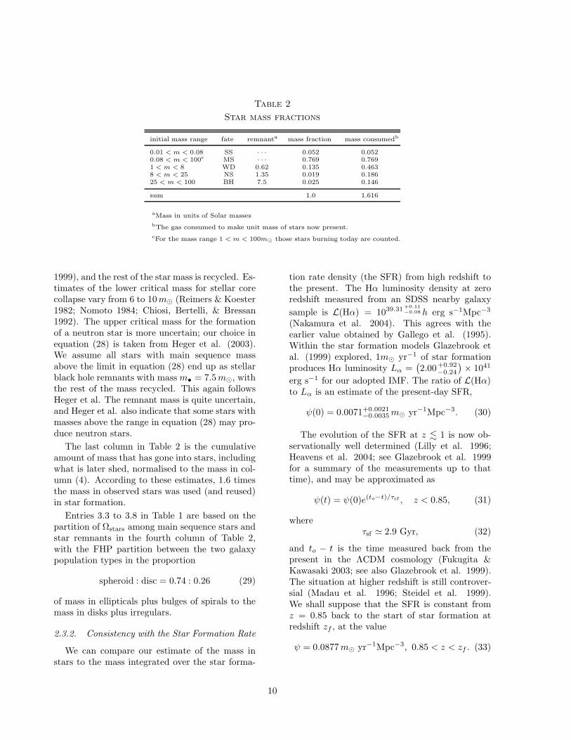
Table 2

Star mass fractions

initial mass range fate remnanta mass fraction mass consumedb

0.01 < m < 0.08 SS · · · 0.052 0.0520.08 < m < 100c MS · · · 0.769 0.7691 < m < 8 WD 0.62 0.135 0.4638 < m < 25 NS 1.35 0.019 0.18625 < m < 100 BH 7.5 0.025 0.146

sum 1.0 1.616

aMass in units of Solar masses

bThe gas consumed to make unit mass of stars now present.

cFor the mass range 1 < m < 100m⊙ those stars burning today are counted.

1999), and the rest of the star mass is recycled. Es-timates of the lower critical mass for stellar corecollapse vary from 6 to 10m⊙ (Reimers & Koester1982; Nomoto 1984; Chiosi, Bertelli, & Bressan1992). The upper critical mass for the formationof a neutron star is more uncertain; our choice inequation (28) is taken from Heger et al. (2003).We assume all stars with main sequence massabove the limit in equation (28) end up as stellarblack hole remnants with mass m• = 7.5m⊙, withthe rest of the mass recycled. This again followsHeger et al. The remnant mass is quite uncertain,and Heger et al. also indicate that some stars withmasses above the range in equation (28) may pro-duce neutron stars.

The last column in Table 2 is the cumulativeamount of mass that has gone into stars, includingwhat is later shed, normalised to the mass in col-umn (4). According to these estimates, 1.6 timesthe mass in observed stars was used (and reused)in star formation.

Entries 3.3 to 3.8 in Table 1 are based on thepartition of Ωstars among main sequence stars andstar remnants in the fourth column of Table 2,with the FHP partition between the two galaxypopulation types in the proportion

spheroid : disc = 0.74 : 0.26 (29)

of mass in ellipticals plus bulges of spirals to themass in disks plus irregulars.

2.3.2. Consistency with the Star Formation Rate

We can compare our estimate of the mass instars to the mass integrated over the star forma-

tion rate density (the SFR) from high redshift tothe present. The Hα luminosity density at zeroredshift measured from an SDSS nearby galaxy

sample is L(Hα) = 1039.31+0.11

−0.08 h erg s−1Mpc−3

(Nakamura et al. 2004). This agrees with theearlier value obtained by Gallego et al. (1995).Within the star formation models Glazebrook etal. (1999) explored, 1m⊙ yr−1 of star formationproduces Hα luminosity Lα =

(

2.00+0.92−0.24

)

× 1041

erg s−1 for our adopted IMF. The ratio of L(Hα)to Lα is an estimate of the present-day SFR,

ψ(0) = 0.0071+0.0021−0.0035m⊙ yr−1Mpc−3. (30)

The evolution of the SFR at z . 1 is now ob-servationally well determined (Lilly et al. 1996;Heavens et al. 2004; see Glazebrook et al. 1999for a summary of the measurements up to thattime), and may be approximated as

ψ(t) = ψ(0)e(to−t)/τsf , z < 0.85, (31)

whereτsf ≃ 2.9 Gyr, (32)

and to − t is the time measured back from thepresent in the ΛCDM cosmology (Fukugita &Kawasaki 2003; see also Glazebrook et al. 1999).The situation at higher redshift is still controver-sial (Madau et al. 1996; Steidel et al. 1999).We shall suppose that the SFR is constant fromz = 0.85 back to the start of star formation atredshift zf , at the value

ψ = 0.0877m⊙ yr−1Mpc−3, 0.85 < z < zf . (33)

10

In this model the integrated star formation is

Ωstars ≃ 0.0038 if zf = 2,

≃ 0.0047 if zf = 3, (34)

≃ 0.0053 if zf = 5.

There is a significant downward uncertainty,δΩstars ∼ −0.0025, arising from the uncertaintyin the star formation rate (eq.[30]). Equation (27)and Table 2 indicate that the mass processedinto stars, including what was later shed, isΩ = 0.0027 × 1.62 = 0.0044. This is consis-tent with the cumulative star formation in equa-tion (34). There would be a problem with thenumbers if there were reason to believe that theSFR continued to increase with increasing redshiftwell beyond z = 1. A constant or declining SFRat z > 1 is well accommodated with our estimatesfor the baryon budget and current ideas about thestar formation history at high redshift.

The star formation history determines the av-erage reciprocal redshift factor (as in eq. [102])for the effect of redshift on the integrated comov-ing energy density of electromagnetic radiation(and other forms of relativistic mass) generatedby stars. In our model for the SFR the correctionfactor is

〈(1 + z)−1〉−1 =

∫

dtL∫

dtL/(1 + z)

= 2.0 ± 0.15, (35)

where L(t) is the bolometric luminosity densityper comoving volume, which we are assuming isproportional to the star formation rate density.The numerical value assumes the redshift cutoffis in the range zf = 2 to 5. For the purpose ofcomparison of the accumulation of stellar productsto the present rate of production, another usefulquantity represents the integrated comoving den-sity of energy radiated in terms of the effectivetime span normalised by the present-day luminos-ity density,

∆teff = L(t0)−1

∫

dtL(t) = 85 ± 13 Gyr, (36)

The value assume the range of models for the starformation history in equation (34).

We can compare the rate of stellar core collapsein our model to observations of the supernova rate.

(See Fukugita & Kawasaki 2003 and Madau, dellaValle & Panagia 1998 for similar analyses.) Thepresent SFR in equation (30) and the critical min-imum mass 8m⊙ in equation (28) imply that thepresent rate of formation of neutron stars and stel-lar black holes is expected to be

R =

∫ 100

8 dm dN/dm∫ 100

0.08dm m dN/dm

= 0.0079+0.0024−0.0039 (100yr)−1Mpc−3. (37)

Our estimate of the observed supernova rate is

RSN = 0.0076+0.0064−0.0020 (100yr)−1Mpc−3. (38)

This is the geometrical mean of the rates fromthree surveys for Type II and Type Ib/c su-pernovae, 0.037, 0.018 and 0.017, in units ofh3(100yr)−1Mpc−3 (Tammann, Loffler & Schroder1994; Cappellaro et al. 1997; van den Bergh & Mc-Clure 1994; see also Cappellaro, Evans & Turatto1999). We conclude that, if most stars with initialmasses greater than about 8m⊙ produced TypeII and Ib/c supernovae, then our model for thestar formation history would pass this consistencycheck.

We remark that in our model the comovingnumber density of supernovae of types II and Ib/cintegrated back to the start of star formation is

R∆teff = 7 ± 3 × 106 Mpc−3, (39)

where the effective time span is given in equation(36).

2.3.3. Planets and Condensed Matter

The mass in planets that are gravitationallybound to stars must be small, but it is of partic-ular interest to us as residents of a planet. Marcy(private communication; see also Marcy & Butler2000) finds that about 6.5% of nearby FGKM starshave detected Jovian-like planets, and that an ex-trapolation to planets at larger orbital radii mightbe expected to roughly double this number. Inour model for the PDMF the ratio of the numberdensity of stars in the mass range 0.08 to 1.6 m⊙

to the mass density in stars is n/ρ = 2.1m−1⊙ . The

product of this quantity with the mass density instars (eq. [27]), the fraction 0.13, and the ratio ofthe mass of Jupiter to the Solar mass is

Ωplanets = 10−6.1. (40)

11

Marcy indicates that stars with lower metallicityhave fewer planets, but that may not introduce aserious error because there are fewer low metallic-ity stars.

There is a population of interstellar planets thathave escaped from stars that have rapidly shedconsiderable mass. If the number of planets perstar is independent of the stellar mass then, inour IMF, stars in the mass range 1 to 1.6m⊙ had0.025 times the number of stars that are bound tomain sequence stars. Among them about 2/3 arelikely to be swallowed by the host stars in their gi-ant star phases. This leaves the mass in liberatedplanets, and those still bound to white dwarfs,at about 0.07 times the mass density in equa-tion (40). Planets associated with more massivestars may more likely escape during core collapse,but the numbers of stars, and perhaps planets, issmall. The large uncertainty in equation (40) iswhether the stellar neighborhood is a fair sample.This leads us to enter the order of magnitude inTable 1.

We consider separately the mass in objectssmall enough to be held together by molecularbinding energy rather than gravity. The dom-inant amount of the former is interstellar dust.It is known (Draine 2003) that & 90% of siliconatoms in interstellar matter are condensed intograins, probably dominantly in the forms of en-statite (MgSiO3) and forsterite (Mg2SiO4) withthe former likely three to four times more abun-dant (Molster et al. 2002). This means the mass inthis form is Z(silicates)/Z = 0.17 times the massin heavy elements. Draine (2003) suspects that thedominant contribution to the carbonaceous mate-rial is in the form of polycyclic aromatic hydrocar-bon with the inferred abundance C/H=6×10−5.Adding this to the silicates, we find that the massfraction becomes Z(dust)/Z = 0.20. The for-mation of dust with iron or other forms of car-bonates could increase this number. Entry 3.12,Ωdust = 10−5.6, is the product of the density pa-rameter in cool gas (entries 3.9 plus 3.10) with themean metallicity discussed below (and displayedas eq. [88]) and the 20 percent heavy element massfraction in dust. Our estimate, which assumesthat what we know about the Milky Way appliesto other galaxies, is crude, but it seems likely thatthe mass in dust exceeds the mass in planets.

There are larger objects in which molecular

binding is important. The gravitational bindingenergy of a roughly spherical object with mass mand radius r is ∼ Gm2/r, and the molecular bind-ing energy is roughly 1 eV per atom. The molecu-lar binding energy is larger than the gravitationalenergy when

m . 1.2 × 1028 g (5 g cm−3/ρ)1/2/A, (41)

where the mass density is ρ and the mean atomicweight is A. For silicates, this bound is m =8 × 1026 g. That is, gravitational binding energydominates in the Earth and molecular binding en-ergy dominates in the Moon and asteroids. Tru-jillo, Jewitt, & Luu (2001) estimate that the massin the Kuiper Belt objects is about a tenth of anEarth mass, or 10−6.5m⊙. A comparable mass isin the moons in the Solar system. If this massfraction were common to all stars the density pa-rameter in these objects would be

Ωasteroid ∼ 10−9, (42)

a small fraction of the mass in dust.

2.3.4. Neutral Gas

The recent blind HI surveys are a significantadvance over the data used by FHP to estimate themass density in neutral atomic gas. The largestsurvey, HIPASS, with 1000 galaxies (Zwaan et al.2003), gives

ΩHI = 4.2 ± 0.7 × 10−4. (43)

The increase over the value quoted in FHP (1.5times the upper end value of FHP) illustrates theadvantage of blind surveys over observations ofprogrammed galaxies. The molecular hydrogenabundance from the CO survey of Keres, Yun &Young (2003) is

ΩH2= 1.6 ± 0.6 × 10−4. (44)

The sum of these two values is multiplied by 1.38to accommodate helium.

We place in entry 3.9 the atomic hydrogen andthe helium abundance belonging to atomic andmolecular hydrogen. Entry 3.10 is the molecularhydrogen component. The mass in this neutralgas is 1.7±0.4% of the total baryon mass.

12

2.3.5. Intracluster Plasma

The estimate of the plasma mass in rich clus-ters of galaxies depends on a convention for thecluster radii and masses. We use the mass M200

contained by the nominal virial radius, r200. Thisdefinition is more faithful to a physical definitionof the part of a cluster that is close to dynamicalequilibrium, and it also traces the X-ray radiuswhich is the definition of our hot gas. In the lim-iting isothermal sphere model the relation to themass within the Abell radius rA = 1.5h−1 Mpc is

MA = M1/3o M

2/3200 , Mo = 1.1 × 1015m⊙. (45)

This agrees with the estimates of the two massesgiven by Reiprich & Bohringer (2002), Table 4.We adopt the Reiprich & Bohringer cluster massdensity parameter,

Ωcl = 0.012+0.03−0.04, (46)

for the cluster mass limit

M200 > 5×1013m⊙, MA > 1.3×1014m⊙. (47)

That is, 4% of the mass is assembled in rich clus-ters. The Bahcall & Cen (1993) Abell mass func-tion is consistent with the Reiprich & Bohringerestimate. We caution that the Bahcall et al.(2003) SDSS mass function is about half what weadopt, perhaps because SDSS samples a subset ofthe clusters. Note also that the integral over thecluster mass within the Abell radius gives a sub-stantially larger value for Ωcl because MA > Mo

at the masses M & 1014m⊙ that dominate theintegral for a given mass function.

The abundance of hot baryons in clusters is ob-tained from the expression

Ωb,cl = 0.012(Ωb − Ωstars)/Ωm

= 0.0018 ± 0.0007. (48)

The change from the value in FHP is mainly dueto the definition of the cluster mass, as also notedby Reiprich & Bohringer.

2.3.6. Massive Black holes

We follow the standard idea that the massiveobjects in the centers of galaxies are black holesthat formed by the accretion of baryons. Baryonsentering black holes are said to lose their identity,

but for our accounting it is appropriate to considerthem to be sequestered baryons.

We define the characteristic efficiency factor ǫnfor black hole formation (where the subscript ismeant to distinguish the massive black holes in thecenters of galaxies from stellar mass black holes)by the black hole mass produced out of an initialdiffuse baryon mass mb,

mbh = (1 − ǫn)mb, (49)

where the energy released in electromagnetic radi-ation, neutrinos, kinetic energy, and possibly grav-itatonal radiation is

memitted = ǫnmb. (50)

The baryon mass sequestered in massive blackholes, mb = mbh/(1 − ǫn), could be substantialif ǫn were close to unity. However, if an appre-ciable part of the binding energy were released aselectromagnetic radiation then the bounds on theradiation background (in category 7) and thoseof the CMBR distortion (eq. [15]) would requirethat the energy was released at very high redshift,kT > 107 K. The estimates discussed in §2.7.6 in-dicate the mass fraction released in gravitationalradiation is small. Thus it seems likely that ǫn issmall, as is assumed in entry 3.13. The efficiencyfactor ǫs typical of stellar mass black holes doesnot appear in entry 3.7, because this estimate isbased on an analysis of the progenitor star masses.The estimate of the mean mass density in massiveblack holes that is used for entry 3.13 is discussedin §2.5.3.

2.3.7. Intergalactic Plasma

Entry 3.1, for the baryon mass outside galaxiesand clusters of galaxies, is the difference betweenour adopted value of the baryon density parame-ter (eq. [17]) and the sum of all the other entriesin category 3. Within standard pictures of struc-ture formation this component could not be in acompact form such as planets, but rather mustbe a plasma, diffuse enough to be ionized by theintergalactic radiation or else shocked to a tem-perature high enough for collisional ionization, butnot dense and hot enough to be a detectable X-raysource outside clusters and hot groups of galaxies.

In our baryon budget 90% of the baryons are inthis intergalactic plasma. It is observed in several

13

states. Quasar absorption lines show matter inlow and high atomic ionization states in the halosof L ∼ L∗ galaxies, extending to radii ∼ 200 kpc(Chen et al. 2001 and references therein). Ab-sorption lines of HI and MgII reveal low surfacedensity photoionized plasma at kinetic tempera-ture T ∼ 104 K, which can be well away fromL ∼ L∗ galaxies, as discussed by Churchill, Vogt,& Charlton (2003), and Penton, Stocke & Shull(2004). The latter authors estimate that 30% ofthe baryons are in this state. Absorption linesof O VI around galaxies and groups of galaxies(Tripp, Savage & Jenkins 2000; Sembach et al.2003; Shull, Tumlinson, & Giroux 2003; Richteret al. 2003), reveal matter that may be excitedby photoionization by the X ray background ra-diation and by collisions in plasma at the kinetictemperature T ∼ 106 K characteristic of the mo-tion of matter around galaxies (Cen et al. 2001).The detection of O VII and O VIII absorption linesalso indicates the presence of higher temperatureregions in the local IGM (Fang et al. 2002; Fang,Sembach & Canizares 2003). Improvements in theconstraints on the amount of matter in these vari-ous states of intergalactic baryons will be followedwith interest.

For the inventory we adopt the measure ofthe concentration of dark matter around galaxiesin equation (13), and the argument discussed in§ 2.3.8 that the baryons are distributed like thedark matter on scales comparable to the virialradii of galaxies. The resulting division into themass in baryons near the virial radii of normalgalaxies outside clusters (entry 3.1a), and the masswell away from galaxies and compact groups andclusters of galaxies (entry 3.1b), is presented assub-components, because the sum is much betterconstrained than the individual values.

2.3.8. Baryon Cooling

We comment here on a simple picture for thecooling and settling of baryons onto galaxies. Thesum of the baryon mass densities belonging togalaxies, in entries 3.3 to 3.13, is Ωb,g = 0.0035.This is 8% of the total baryon mass. SupposeΩb,g consists of all baryons gathered from radiusrg around L ∼ L∗ galaxies, and suppose we canneglect the addition of baryons by settling fromfurther out and the loss by galactic winds. Thatis, we are supposing that at r > rg the ratio of the

baryon density to the dark matter density is thecosmic mean value, and that the baryons closerin have collapsed onto the galaxies. In this pic-ture the characteristic radius of assembly of thebaryons satisfies

2ngrgσ2

Gρm=

Ωb,g

Ωb,total, (51)

in the limiting isothermal sphere approximation(eq. [9]).

In equation (51) ng is a measure of the numberdensity of luminous galaxies. We record here ourchoices for this quantity and related parametersthat are used elsewhere. We take

ng = Lr/L∗r = 0.017h3 Mpc−3, (52)

where Lr is the luminosity density (eq. [14]). Thecharacteristic galaxy luminosity,

L∗B = 1.07 × 1010h−2L⊙,

L∗r = 1.45 × 1010h−2L⊙, (53)

L∗z = 2.37 × 1010h−2L⊙,

is the luminosity parameter in the Schechter func-tion, with the power law index αB = −1.1, αr =−1.13, and αz = −1.14. We refer some estimatesof energy densities to what is known about theMilky Way, for which we need the effective num-ber density of Milky Way galaxies. In the B bandthe Milky Way luminosity is LMW = 1.3L∗

B, andthe effective number density is

nMW = LB/L∗MW = 0.013h3 (Mpc)−3. (54)

Almost the same density follows when referred tothe r-band. The Milky Way parameters are dis-cussed in the Appendix.

With the characteristic velocity dispersion inequation (10) and the characteristic galaxy num-ber density in equation (52) the baryon accretionradius defined by equation (51) is

rg ≃ 30h−1 kpc, (55)

at density contrast 1.3 × 104 and plasma den-sity ngas(rg) ∼ 0.007h3 cm−3. If plasma at thisradius were supported by pressure at the one-dimensional velocity dispersion σ ≃ 160 km s−1

in equation (10) the temperature would be T ≃2 × 106 K. At this density and temperature the

14

thermal bremsstrahlung cooling time would beshort enough, ∼ 4 × 109 yr, that stars would haveformed and disks matured at z ∼ 1.

We have lower bounds on the cooling radiusfrom the observation that the neutral atomic hy-drogen density around L∗ galaxies reaches NHI =1.8×1020 cm−2 at the effective radius ∼ 20h−1 kpc(Bosma 1981), and Mg II absorption lines are ob-served at radius ∼ 40h−1 kpc (Steidel, Dickinson& Persson 1994). For the Milky Way the distri-bution of RR Lyr stars cuts off sharply at 50 kpc(Ivezic et al. 2000). The cooling radius must belarger than these indicators of relatively cool mat-ter. Equation (55) is not inconsistent with thiscondition. Though the history of baryon accre-tion by galaxies undoubtedly is complex, we canimagine, as a first approximation, that a substan-tial fraction of the baryons now concentrated ingalaxies are there because they were able to cooland settle from an initial distribution similar tothat of the dark matter.

The relative distributions of baryons and darkmatter at distances much larger than rg fromgalaxies might not be greatly disturbed from theprimeval condition. If so, then the product of thebaryon density parameter with the virialized darkmatter mass fraction in equation (13) is an esti-mate of the baryon mass that resides within thevirial radii of normal galaxies, and the remainder,

Ωb,ig ∼ 0.016, (56)

which is presented as entry 3.1b, would be locatedoutside galaxies and remain less than fully docu-mented.

2.4. Primeval Gravitational Energy

In the ΛCDM cosmology the gravitational bind-ing energy of the present mass distribution has twocontributions. The first, which we term primeval,is a result of the purely gravitational growth ofmass fluctuations out of the small adiabatic de-partures from a homogeneous mass distributionpresent in the initial conditions for the Friedmann-Lemaıtre cosmology. The second, to be discussedin the next subsection, is the result of dissipa-tive settling of baryons that produced the baryon-dominated luminous parts of the galaxies alongwith stars and star remnants. We can find sensi-ble approximations to the primeval and dissipative

components because, as we will discuss, the char-acteristic length scales are well separated.

The primeval gravitational energy is defined byimagining a universe with initial conditions identi-cal to ours in all respects except that the baryonicmatter in our universe is replaced by an equal massof CDM in the reference model. At the presentworld time this reference model contains a clus-tered distribution of massive halos with gravita-tional binding energy density that we term theprimeval component.11 This component is esti-mated as follows.

The Layzer (1963) - Irvine (1961) equation forthe evolution of the kinetic and gravitational ener-gies of nonrelativistic matter, such as CDM, thatinteracts only by gravity is

d

dt(K +W ) +

a

a(2K +W ) = 0. (57)

The kinetic energy per unit mass is

K = 〈m~v 2/2〉/〈m〉, (58)

where ~v is the peculiar velocity of a particle withmass m. The gravitational potential energy perunit mass is

W = −1

2Gρm

∫

d3r ξ(r)/r, (59)

where ρm is the mean mass density and ξ is thereduced mass autocorrelation function.

We can use a simple limiting case of the Layzer-Irvine equation, because in the ΛCDM cosmology

11One surely would say that in this model universe the viri-alized dark matter halos have gravitational binding energy.Since there was no energy transfer to some other form, onemight also want to say that this binding energy must havebeen present in the initial conditions. Furthermore, one canassign to a linear mass density fluctuation with contrastδ(t) > 0, and comoving radius x (physical radius xa(t)),a gravitational energy per unit mass, W ′ ∼ −G〈ρ〉δ(ax)2 ,which is constant in linear perturbation theory and com-parable to the binding energy of the final virialized halo.Perhaps one can use this as a guide to a definition of theprimeval energy belonging to the density fluctuation, de-spite the problem that the mean of W ′ vanishes, and thefact that in general relativity theory there is no generaldefinition of the global energy density of a statistically ho-mogeneous system. We have not been able to find a usefulapproach along these lines. We might add that if our uni-verse had been Einstein-de Sitter then we would have de-fined the primeval energy density by a numerical solutionof equation (57).

15

the universe has now entered Λ-dominated expan-sion, which has caused a significant suppression ofthe rate of growth of large-scale departures fromhomogeneity. This means that the first term inequation (57) has become small compared to thesecond term. Thus it is a reasonable approxima-tion to take 2K = −W , the usual virial equilib-rium relation. Then the gravitational binding en-ergy per unit mass is U = K + W = W/2, andthe cosmic mean primeval gravitational bindingenergy is the product of U with the mean massdensity Ωm in matter (eq. [8]). With the normal-

ization P (k) =∫

d3r ξ(r)ei~k·~r for the mass fluc-tuation power spectrum, the expression for theprimeval gravitational binding energy in this ap-proximation is

ΩBE,p = −3Ω2

mH2o

16π2

∫ ∞

o

dk P (k). (60)

For a numerical value we use the mass fluctua-tion power spectrum P (k) in Figure 37 of Tegmarket al. (2004b) at k < 0.1h Mpc−1. At smallerscales the Tegmark et al. spectrum decreases toorapidly with increasing wavenumber k to be a goodapproximation to the present mass distribution(Davis & Peebles 1983). We approximate the spec-trum as

P (k) = 7000

(

0.1h Mpc−1

k

)1.23

h−3 Mpc3, (61)

at k > 0.1h Mpc−1. This is based on the Fouriertransform of the pure power law model for thegalaxy autocorrelation function (eq. [5]),

P = 4πrγok

γ−3Γ(2 − γ) sinπ(2 − γ)/2, (62)

which gives P = 5200h−3 Mpc3 at k = 0.1hMpc−1.We choose the somewhat larger normalization inequation (61) to fit the SDSS measurement. Thenumerical result is

∫ ∞

o

P (k) dk = 4800h−2 Mpc2. (63)

The integral of the Tegmark et al. (2004b) powerspectrum over all wavenumbers is 2700h−2Mpc,which is 0.55 times the value in equation (63). Ourestimate of the integral is based on measurementsof the actual power spectrum, not the spectrumthat would have obtained if there were no dissi-pative settling of baryons, but the error is small

because the integral is dominated by lengths largecompared to the scale of separation of baryonsfrom the dark matter.

Equations (60) and (63) yield the entry in line4 of Table 1,

Ωgrav,p = −7.7 × 10−7. (64)

This is the density parameter of the gravitationalbinding energy of the present departure from ahomogeneous mass distribution, ignoring the ef-fects of the dissipative settling of baryons. It willbe useful to note that a measure of the lengthscale of the gravitational energy is the half-pointof the integral in equation (63), at wavenumberk1/2 = 0.27h Mpc−1, or half wavelength

λ1/2 = π/k1/2 = 12h−1 Mpc. (65)

The kinetic energy per unit mass belonging toequation (64) is

K = −U = 3(410 km s−1)2/2. (66)

The velocity in parentheses is the one-dimensionalsingle-particle line-of sight rms peculiar velocity.

The gravitational binding energy is not equal toa sum over the contributions from individual ob-jects, but we can write useful approximations tothe decomposition into the three components —the virialized parts of the massive halos of L ∼ L∗

galaxies, the rich clusters, and large-scale cluster-ing — shown in category 4 in the inventory.

Since galaxy rotation curves tend to be close toflat we write the binding energy of the virializedparts of the dark matter halos of the galaxies as

Ωgrav = −3Ωmσ

2

2

ρ(rv)

ρm= 10−7.2, (67)

where Ωm is the matter density parameter (eq. [8]),σ is the characteristic velocity dispersion in equa-tion (10) and the last factor is the virialized massfraction (eq. 13). This is about 10% of the to-tal gravitational binding energy. The dissipativesettling that produced the baryon-dominated lu-minous parts of the galaxies would have perturbedthe massive halos, but the disturbance to theprimeval gravitational energy is small because thebaryon mass fraction is small.

Our estimate of the binding energy of the darkhalos of the galaxies may be compared to the den-sity parameter given by equation (60) when the

16

integral over P (k) is restricted to small scales,k > π/rv, where rv is the virial radius in in equa-tions (10) and (67). The result, with equation (61)for P (k), is twice the value in equation (67). Thedifference is an indication of the ambiguity of sep-arating gravitational energy into components. Forentry 4.1 we adopt the value in equation (67) asthe more directly interpretable.

Equation (67) is a reasonable approximation formost of the mass in galaxy-size dark halos in lu-minous field galaxies such as the Milky Way, butin rich clusters the galaxies tend to share a darkhalo that is close to smoothly distributed acrossthe cluster. Our estimate in entry 4.2 for theprimeval gravitational binding energy belonging torich clusters follows equation (67), with σ = 800km s−1 and Ωcl from equation (46). Rich clustersshare about 15% of the total gravitational bindingenergy.

Entry 4.3 is the difference between the total inentry 4 and the sum of entries 4.1 and 4.2. TheLayzer-Irvine equation indicates that the bindingenergy is dominated by a length scale (eq. [65])that is much larger than galaxy virial radii. Con-sistent with this, entry 4.3 is larger than entry 4.1for the binding energy of the dark halos of galax-ies. The difference is not large, however, becauseat small scales the integral over the power spec-trum converges slowly, as k−0.23.

2.5. Dissipative Gravitational Settling

Dissipative settling has increased the magni-tude of the gravitational binding energy from thatprescribed by the primeval conditions consideredin the last section. In §2.5.1 we discuss the energyreleased in producing the increased mean densityof baryons relative to dark matter in the lumi-nous parts of the galaxies, in §2.5.2 we estimatethe gravitational energy released in stellar forma-tion and evolution, and in §2.5.3 we consider thecentral massive compact objects in galaxies.

2.5.1. The Luminous Parts of Galaxies

In the Milky Way galaxy the mass within ourposition, at about 8 kpc from the center, is roughlyequal parts baryonic and dark matter, or about 6times the cosmic mean ratio (eq. [19]). This isthought to be the usual situation in the luminousparts of normal galaxies. The amount of gravi-

tational binding energy released in producing thisconcentration of baryons depends on how it wasdone. In one limiting case one may imagine thatstars formed in the centers of low mass dark haloswith relatively small dissipation of energy — apartfrom star formation — because the depths of thegravitational potential wells were small, and thatthe low mass halos later merged without any ad-ditional dissipation, the dense baryon-dominatedparts remaining near the densest regions to formthe present-day baryon-dominated luminous partsof galaxies. (This is an extreme version of thescenario discussed by Gao et al. 2003). In an-other extreme, one may imagine that the baryonssettled into previously assembled galaxy-scale ha-los, which would dissipate considerably more en-ergy. A galaxy has a definite computable gravi-tational binding energy, of course (apart from thedifficulty of correcting for ongoing accretion), butto relate this to the energy dissipated in producingthe galaxy would require an analysis of what themass distribution would have been in the absenceof dissipation, which is not an easy task.

These considerations lead us to offer only acrude estimate for entry 5.1, which we write asthe product of the density parameter belonging tobaryons in galaxies — the sum Ωb,g = 0.0035 ofthe density parameters in entries 3.3 to 3.13 —with the kinetic energy per unit mass, K = 3σ2/2and σ = 160 km s−1. The result is a 2% ad-dition to the primeval halo gravitational bindingenergy (entry 4.1). If the baryon concentrationsin galaxies formed at high redshifts in small halosthe dissipative energy released would be an evensmaller fraction of the total.

2.5.2. Stellar Binding Energy

The amount of binding energy released in starformation is easy to define because the relativelength scale is small. We write the gravitationalbinding energy per unit mass for a star with massm and radius r as

BE

m= −K

Gm

rc2. (68)

The prefactor for the Sun is K⊙ = 1.74, and K =0.3 for a homogeneous sphere.

For main sequence stars we use the zero-agemass-radius relation, r ≃ 0.85m0.80 for 0.08 <m < 0.79, r ≃ 0.93m1.17 for 0.79 < m < 1.38,

17

and r ≃ 1.15m0.52 for 1.38 < m < 100, in so-lar units. These numbers are assembled from Ezer& Cameron (1967), Cox & Giulli (1968) and Cox(2000). Integration of Gm2/r over the PDMFgives BE/m = 3.7×10−6. The product of the lastnumber with the density parameter of the massin main sequence stars (entries 3.3 plus 3.4), withK ≃ K⊙, is the estimate of the gravitational bind-ing energy, ΩBE = −10−8.1, for stars. We similarlyobtain the substellar gravitational binding energy,ΩBE = −10−9.6, where r is fixed at 0.096 r⊙ (Bur-rows et al. 2001). This is a small addition to thesum in entry 5.2.

We construct a model for the white dwarf massfunction from an approximation to the relation be-tween the progenitor main sequence mass and thewhite dwarf remnant mass (Claver et al. 2001;Weidemann 2000),

mwd = 0.08mms + 0.45m⊙, (69)

and our IMF. White dwarf masses run from0.53 to 1.09m⊙ for the main sequence massrange 1 < mms < 8m⊙ we have adopted.The white dwarf mass function dN/dmwd =(dN/dmms)(dmms/dmwd) thus obtained agreeswell with the observed white dwarf mass distri-bution of Bergeron & Holberg for m & 0.5m⊙ (inpreparation). Here we ignore low mass heliumcore white dwarfs. In our mass function the meanwhite dwarf mass is

〈mwd〉 = 0.62m⊙. (70)

From our mass function and the mass-radius re-lation given by Shapiro and Teukolsky (1983) weobtain the mean white dwarf gravitational bindingenergy per unit mass,

BE

m= −58Kwd

Gm⊙

r⊙c2= −1.2 × 10−4. (71)

Since the fractional half-mass radius of a whitedwarf is 0.57 times the solar value (Schwarzschild1958), we have taken Kwd ≃ 1.0. The productwith the mass density in white dwarfs (entry 3.5)is entry 5.3.

We take the binding energy of a neutron starto be 3 × 1053 erg (e.g., Burrows 1990; Janka &Hillebrandt 1989), or

BE/m = −0.12. (72)

The product with entry 3.6 is entry 5.4, ΩBE,NS =10−5.2. The gravitational binding energies in neu-tron stars and stellar mass black holes are sub-stantially larger than the gravitational binding en-ergies in all other forms.

2.5.3. Black Hole Binding Energy

Our definition of the binding energy associatedwith a black hole requires careful explanation be-cause it has some curious properties, including vi-olation of the thought that it would be logical toconsider the mass of a black hole to be purely grav-itational if the matter out of which it formed haslost its existence.

We choose the definition by analogy to nuclearand Newtonian gravitational binding energy, interms of the energy liberated in the assembly ofa system out of its initial parts, that is, the dif-ference between the total mass of the initial partsand the mass of the assembled system. In the sameway, we use equations (49) and (50) to define thebinding energy of a black hole by the difference be-tween the mass mb of the initial parts — baryons— and the mass mbh = (1 − ǫn)mb of the finalblack hole. Thus our definition of the binding en-ergy of a black hole is

BE = −ǫnmb = −ǫn

1 − ǫnmbh. (73)

The magnitude of BE is the energy emitted aselectromagnetic and gravitational radiation, neu-trinos, and kinetic energy, as is appropriate for ourpurpose of telling the energy transfers and balanc-ing the baryon budget. It will be noted that inthis definition the binding energy depends on howthe black hole formed. For example, a Solar massblack hole that formed with efficiency ǫ = 0.99is assigned binding energy −99m⊙, because it re-leased that much energy, while an identical blackhole that formed with ǫn = 0.01 is assigned a verydifferent binding energy, −0.01m⊙.

Entry 5.5 for the gravitational binding energyof stellar mass black holes is the product of entry3.7, which is our estimate of the baryonic massentering the black hole, with the efficiency fac-tor ǫs. In the standard picture for the formationof a stellar mass black hole, a core of baryons isfirst burned to heavy elements, and the subsequentcollapse to a black hole may release little more en-ergy. In this case the efficiency factor could be as

18

small as ǫs ∼ 0.009, which is the binding energyreleased as starlight. It could also be as large asǫs ∼ 0.03 if the collapse proceeded through a pro-toneutron star as an intermediate state. It can-not be much larger, however, without violatingthe constraints from the radiation energy density(see §2.7) and the relic supernova neutrino flux atSuper-Kamiokande (Fukugita & Kawasaki 2003).

One way to estimate the mass density in themassive black holes in the nuclei of galaxies usesthe correlation of the black hole mass with thebulge luminosity. A convenient approximation tothe relation, for B-band luminosities, is (Gebhardtet al. 2000; Ferrarese 2002; see also Kormendy &Richstone 1995)

M•/m⊙ = 10−2.0±0.3Lbulge/L⊙. (74)

FHP estimate that the fraction of the B-band lu-minosity density in ellipticals and S0 galaxies is0.24, and the fraction in the bulges of spheroidsis 0.14. The products of equation (74) with theluminosity fractions and the luminosity density inequation (14) gives the mass density parametersin massive black holes,

Ω•(early) = 10−5.6±0.3,

Ω•(late) = 10−5.9±0.3. (75)

Salucci et al. (1999) give a consistent, but slightlylarger value.

For early-type galaxies we can use the tight re-lation between the black hole mass and the bulgeor spheroid velocity dispersion (Merritt & Fer-rarese 2001; Tremaine et al. 2002). The Shethet al. (2003) estimate of the velocity dispersionfunction for early-type galaxies is

dN = φ∗

(

σ

σ∗

)αβ

Γ(α/β)

dσ

σe−(σ/σ∗)β

, (76)

with α = 6.5, β = 1.93, σ∗ = 89 km s−1,φ∗ = 0.0020 Mpc−1. The Tremaine et al. (2002)estimate of the black hole mass-velocity dispersionrelation is

M• = B(σ/σh)a, (77)

with B = 1.3 × 108m⊙, a = 4.0, and σh = 200km s−1. The product of the two expressions, inte-grated over σ, gives the mean mass density,

ρ• = Bφ∗Γ((α + a)/β)

Γ(α/β)

(

σ∗σh

)a

. (78)

The numerical result,

Ω•(early) = 10−5.9, (79)

is close to but smaller than the more direct esti-mate in equation (75). Although the formal un-certainty in equation (79) is smaller it rests on thecondition that the Sheth et al. galaxies are a fairsample of the early-type galaxies, which will re-quire careful debate.12 Thus in the inventory wequote equation (75).

2.5.4. Quasar Luminosities and Remnants

So ltan (1982) and Chokshi & Turner (1992)have considered the relation between the rate ofradiation of energy by quasars and AGNs and theaccumulation of mass in the quasar engines, whichare assumed to be massive black holes in the cen-ters of galaxies. In this repetition of the calcula-tion we take the number of quasars per unit lumi-nosity and comoving volume to be

L∗dn

dL=

L∗Φ(L∗)

(L/L∗)α + (L/L∗)β, (80)

where, from Croom et al. (2004), α = 3.31, β =1.09,

L∗Φ(L∗) = 1.81 × 10−6 Mpc−3, (81)

and the present characteristic luminosity is

L∗ = 6.7 × 1010LB(⊙). (82)

In the Croom et al. luminosity evolution modelthis luminosity evolves as L∗(z) ∝ 101.39z−0.29z2

to redshift z = 2.1, the deepest redshift used in theCroom et al. analysis. The peak of the observedcomoving quasar number density is at z ≃ 2.5,and at 2.5 < z < 5 the density varies about asn ∝ e−1.5z (Fan et al. 2001, Fig. 3). As a con-venient approximation to this behavior we adoptthe Croom et al. (2004) luminosity evolution atz < 2.1, constant comoving luminosity densityfrom z = 2.1 to z = 3, and negligibly small lu-minosity at larger redshifts.

The integral∫

dLL dn/dL is the comoving lu-minosity density, and the time integral multiplied

12The velocity function of Sheth et al. gives 〈σ4〉1/4 = 180km s−1, compared to our estimate of the characteristic ve-locity dispersion, σ∗ = 200 − 220 km s−1, in early-typegalaxies. Perhaps this is related to the difference.

19

by the bolometric correction is the net comov-ing density of energy released. Using the Elviset al. (1994, Table 17) bolometric correction fac-tor BC ≡ Lbol/(νLν)|

4450A= 12, and ignoring

the difference between B and bJ passbands (sincethe quantity that concerns us, νLν for quasars,is close to flat), we estimate that the integratedenergy density released by the quasars is

ΩQSOem = 8 × 10−8. (83)

This uses the solar luminosity,

νLν(⊙) = 2.22 × 1033 erg s−1, (84)

at λ = 4450 A.

Before comparing this estimate to the accu-mulated mass in black holes let us check consis-tency with the integrated background radiation.Equation (83) with the Elvis et al. bolomet-ric corrections indicates that the integrated back-ground from quasars at 100µ < λ < 1000 A isΩ ∼ 3 × 10−8, or 1% of the total (eqs. [106]plus [107] below). To estimate the expected X-ray background we imagine the radiation from thequasars all is emitted at effective redshift z = 2.In this simple model the present energy densityper logarithmic interval of frequency at 2 keV is

νΩν(2 keV) =ΩQSOem

1 + z

νeLνe∫ ∞

0Lνdν

, (85)

where on the right-hand side hνe = 2(1 + z) keV.The mean spectrum in figure 10 in Elvis et al.(1994) for radio-quiet quasars, with the bolometricfactor, indicates that νeLνe

=∫ ∞

0 Lνdν/50 at restframe energy hνe = 6 keV. These numbers give thepresent energy density per logarithmic interval ofphoton energy νΩν = 10−9.3 at 2 keV. The mea-sured value of the X-ray background is (De Luca &Molendi 2004) νΩν = 10−8.8 at 2 keV, about threetimes what is indicated by equations (83) and (85).Since about 80% of the X-ray background at 2 keVis resolved (Mushotzky et al. 2000; Worsley et al.2004), these numbers allow room for a significantpopulation of optically faint quasars.

We turn now to the efficiency ǫn for productionof electromagnetic radiation in the accumulationof the present mass in quasar remnants. If ǫn issmall the estimate of the integrated mass addedto the black holes by the observed energy produc-tion by quasars and AGNs is ∆ΩBH = ΩQSOem/ǫn

(eq. [83]). The ratio of this expression to the massdensity in massive black holes (the sum of entries5.6 and 5.7) is our estimate of the radiation effi-ciency,

ǫn = 0.02. (86)

This is one fifth of the commonly discussed value,ǫn ∼ 0.1. Since our estimate of the X-ray back-ground from optically identified quasars is onethird of the measured value, it may be that equa-tion (83) is low by a factor of about three andequation (86) accordingly low by a like factor. Acloser check of consistency of the idea that themassive black holes in the centers of galaxies arethe quasar remnants awaits advances in surveys ofoptically faint quasars in broader ranges of wave-length and redshift and better understanding ofthe quasar emission mechanism. We may alsohope that future work will establish the natures ofthe sources of the harder X-ray background andthe possible relevance to the black hole mass bud-get.

2.6. Nuclear Binding Energy

2.6.1. Heavy Element Abundances

We consider here the binding energy released bynuclear burning in stars. We normalize the heavyelement abundances to the Solar mass fractions inhydrogen, helium, and heavy elements,

X⊙ = 0.71, Y⊙ = 0.27, Z⊙ = 0.019. (87)

The ratio Z/X = 0.027 is derived (BP2000) as theinitial solar value from (Z/X)solar surface = 0.0230of Grevesse & Sauval (2000), and X is also the ini-tial value of BP2000. The metallicity in star pop-ulations is correlated with the galaxy luminosity.An average over the Schechter luminosity functionof the Kobulnicky & Zaritsky (1999) correlation ofthe oxygen abundance with the B-band galaxy lu-minosity, taking 12 + log(O/H)⊙ = 8.83 (Grevesse& Sauval 2000)13 as the zero point, indicates that

13Recent work on the solar heavy element abundancesuggests a significantly lower oxygen abundance, 12 +log(O/H)⊙ = 8.69 (Allende Prieto, Lambert & Asplund2001), but if the heavy element abundances of other ele-ments are scaled down in a similar manner, as indicatedby the same team, our net result is not affected. In fact,Bahcall and Pinsonneault (2004) give (Z/X)solar surface =0.0176 based on the new abundance, which leaves our resultunchanged.

20

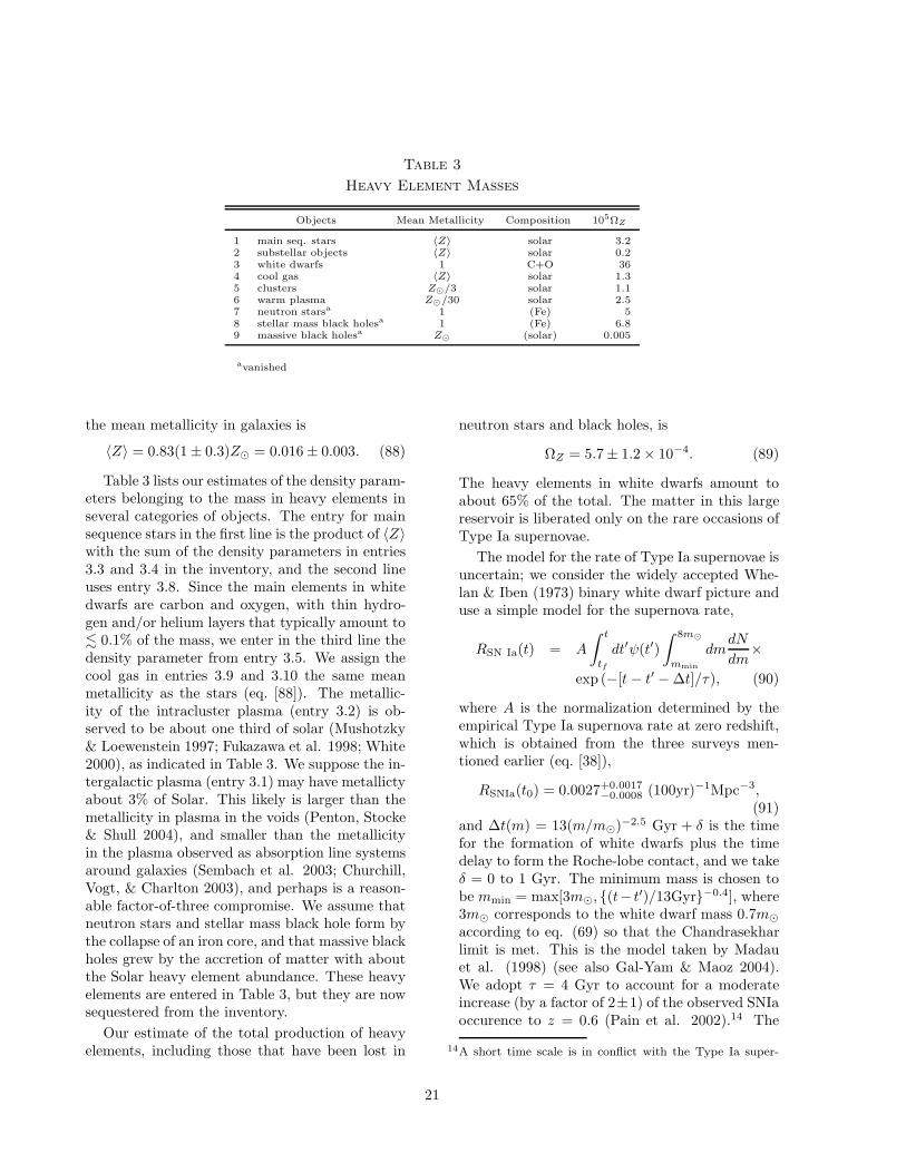
Table 3

Heavy Element Masses

Objects Mean Metallicity Composition 105ΩZ

1 main seq. stars 〈Z〉 solar 3.22 substellar objects 〈Z〉 solar 0.23 white dwarfs 1 C+O 364 cool gas 〈Z〉 solar 1.35 clusters Z⊙/3 solar 1.16 warm plasma Z⊙/30 solar 2.57 neutron starsa 1 (Fe) 58 stellar mass black holesa 1 (Fe) 6.89 massive black holesa Z⊙ (solar) 0.005

avanished

the mean metallicity in galaxies is

〈Z〉 = 0.83(1 ± 0.3)Z⊙ = 0.016 ± 0.003. (88)

Table 3 lists our estimates of the density param-eters belonging to the mass in heavy elements inseveral categories of objects. The entry for mainsequence stars in the first line is the product of 〈Z〉with the sum of the density parameters in entries3.3 and 3.4 in the inventory, and the second lineuses entry 3.8. Since the main elements in whitedwarfs are carbon and oxygen, with thin hydro-gen and/or helium layers that typically amount to. 0.1% of the mass, we enter in the third line thedensity parameter from entry 3.5. We assign thecool gas in entries 3.9 and 3.10 the same meanmetallicity as the stars (eq. [88]). The metallic-ity of the intracluster plasma (entry 3.2) is ob-served to be about one third of solar (Mushotzky& Loewenstein 1997; Fukazawa et al. 1998; White2000), as indicated in Table 3. We suppose the in-tergalactic plasma (entry 3.1) may have metallictyabout 3% of Solar. This likely is larger than themetallicity in plasma in the voids (Penton, Stocke& Shull 2004), and smaller than the metallicityin the plasma observed as absorption line systemsaround galaxies (Sembach et al. 2003; Churchill,Vogt, & Charlton 2003), and perhaps is a reason-able factor-of-three compromise. We assume thatneutron stars and stellar mass black hole form bythe collapse of an iron core, and that massive blackholes grew by the accretion of matter with aboutthe Solar heavy element abundance. These heavyelements are entered in Table 3, but they are nowsequestered from the inventory.

Our estimate of the total production of heavyelements, including those that have been lost in

neutron stars and black holes, is

ΩZ = 5.7 ± 1.2 × 10−4. (89)

The heavy elements in white dwarfs amount toabout 65% of the total. The matter in this largereservoir is liberated only on the rare occasions ofType Ia supernovae.

The model for the rate of Type Ia supernovae isuncertain; we consider the widely accepted Whe-lan & Iben (1973) binary white dwarf picture anduse a simple model for the supernova rate,

RSN Ia(t) = A

∫ t

tf

dt′ψ(t′)

∫ 8m⊙

mmin

dmdN

dm×

exp (−[t− t′ − ∆t]/τ), (90)

where A is the normalization determined by theempirical Type Ia supernova rate at zero redshift,which is obtained from the three surveys men-tioned earlier (eq. [38]),

RSNIa(t0) = 0.0027+0.0017−0.0008 (100yr)−1Mpc−3,

(91)and ∆t(m) = 13(m/m⊙)−2.5 Gyr + δ is the timefor the formation of white dwarfs plus the timedelay to form the Roche-lobe contact, and we takeδ = 0 to 1 Gyr. The minimum mass is chosen tobe mmin = max[3m⊙, (t− t′)/13Gyr−0.4], where3m⊙ corresponds to the white dwarf mass 0.7m⊙

according to eq. (69) so that the Chandrasekharlimit is met. This is the model taken by Madauet al. (1998) (see also Gal-Yam & Maoz 2004).We adopt τ = 4 Gyr to account for a moderateincrease (by a factor of 2±1) of the observed SNIaoccurence to z = 0.6 (Pain et al. 2002).14 The

14A short time scale is in conflict with the Type Ia super-

21

effective time span for the cumulative occurrenceof Type Ia supernovae normalised to the rate atz = 0 is

Teff = RSNIa(t0)−1

∫ t0

tf

RSNIa(t)dt

= 15 ± 3 Gyr, (92)

for our model of star formation (eqs. [31] and [33]with zf = 2.5 to 4). The cumulative comovingnumber density of supernova in this model is 4.0×105 Mpc−3. Since we estimate that the numberdensity of white dwarfs created is 8 × 107 Mpc−3,this would mean that about 1% of the white dwarfshave been disrupted. If 0.7m⊙ of 56Ni is producedin each supernova (e.g., Branch 1992), the massdensity of iron-group elements produced by typeIa supernovae is ΩFe = 2.0× 10−6. This is supple-mented with ΩFe = 3.6× 10−6 from Type II+Ib/csupernovae (see eq. [39]), which produces 0.075m⊙

of iron per event (Arnett 1996; Weaver, Zimmer-man & Woosley 1978). These estimates indicatethat the total density parameter in the iron groupelements is

ΩFe = 6 × 10−6, (93)

of which about 60% is from Type II supernovae.

This estimate can be compared to the productof the mass in heavy elements not locked up instellar remnants (the sum of lines 1, 2, and 4 to 6in Table 3),

Ω′Z = 0.8 ± 0.25 × 10−4 . (94)

with the iron group mass fraction (Grevesse &Sauval 2000),

ΩFe = 0.077Ω′Z = 6.3 × 10−6. (95)

The two approaches give a consistent picture forthe origin of iron and the supernova rates.

nova rates in early type galaxies. With τ = 4 Gyr, theSN fraction in early type galaxies is 0.30 at z ≈ 0, whichis consistent with the observed value, 0.35+0.15

−0.10. Here wehave identified stars formed at z > 0.7 as an early popula-tion that is partitioned into early-type galaxies and bulgesof disk galaxies according to the FHP fractions of bulge lu-minosities. The fraction drops to < 0.25 if τ = 3 Gyr. Theobserved rates of Type Ia supernovae in morphologicallyseparated galaxies seem to be proportional to the r bandluminosity density; the luminosity density in E/S0 galaxiesis 31% of the total (Nakamura et al. 2003). This wouldsuggest a close to constant supernova rate.

The growth of the abundance of heavy elementsis accompanied by the accumulation of helium,apart from the heavy elements that enter whitedwarfs, neutron stars and stellar mass black holes.The estimate of ∆Y/∆Z in equation (20), appliedto all entries in Table 3 except 3, 7 and 8, is ourestimate of the present helium mass fraction inexcess of primeval,

∆ΩY =∆Y

∆ZΩ′

Z = 1.7 ± 1.0 × 10−4. (96)

This is consistent with our estimate from the prod-ucts of stellar evolution (eq. [120]).

There are in the literature many analyses ofthe stellar production of heavy elements (see forexample Calura & Matteucci 2004 and referencestherein). Our results are generally consistent forrelevant entries. Important differences are our in-clusion of heavy elements in white dwarfs, whichdominate the entry, and our consideration of ironin the progenitors of supernovae. These compo-nents are crucial to the consideration of the bal-ance between the nuclear binding energy stored inthe elements and the energy released in radiation.

2.6.2. Nuclear Binding Energies

Our definition of the nuclear binding energiesof the heavy elements differs from the usual prac-tice in tables of nuclei. Because we are interestedin the release of energy in the formation of theheavy elements, we calculate the binding energywith respect to free protons and electrons.

We write the energy released in the productionof the heavy elements present in the interstellarmedium, and in stars when they formed, as

ΩNB, Z = (0.0081 + 0.0071 ∆Y/∆Z)ΩZ, (97)

where 0.0081 is the energy generation efficiencyfactor for the solar composition. The nuclear bind-ing energy in substellar objects and in diffuse mat-ter, in entries 6.2, 6.4, and 6.5 in Table 1, is com-puted from this equation with the heavy elementmasses in Table 3. For main sequence stars, weadd to equation (97) the nuclear binding energyassociated with the helium that has been producedin the stars, which we take to be on average 5%of the star mass, that is, half the helium a starproduces while it is on the main sequence. Thesum is our estimate of the nuclear binding energyin stars in entry 6.1.

22

Entry 6.3, for white dwarfs, is

ΩNB, wd = [0.0080(1 − Yp) + 0.0010Yp]ΩZ

= 10−5.6. (98)

The second term in parentheses accounts for theprimordial helium abundance (eq. [18]). The valueof ΩZ in the first line is taken from line 3 of Ta-ble 3. This component amounts to about 40% ofthe nuclear binding energy. The large amount ofnuclear burning in the stellar giant and supergiantphases is discussed in connection with Table 5 be-low.

The nuclear binding energy in the matter outof which a neutron star formed was converted togravitational binding energy by the dissociationof the heavy elements during a supernova. Thenuclear binding energy released in the formationof the heavy elements that were part of the rawmaterial for a neutron star added to the radiationbackground, of course, but that accounting nowbelongs in category 5. The total entered in theinventory for category 6 accordingly is about 15%smaller than the sum of the nuclear binding ener-gies in all entries in Table 3. The nuclear bind-ing energy to compare to the energy required toproduce the radiation background is the full sum,including iron core progenitors for neutron starsand black holes,

ΩNB = −5.7 ± 1.3 × 10−6. (99)

We discuss the relation to the energy density inradiation in the next subsection.

2.7. The Radiation Backgrounds

The cosmic energy density in electromagneticradiation is thought to be dominated by mildlyredshifted starlight, at λ ∼ 1µ, and a far infraredpeak at λ ∼ 100µ that is produced by the ab-sorption and reradiation of starlight and the lightfrom AGNs (Hauser & Dwek 2001 and referencestherein). The energy densities at radio and X-rayto γ-ray wavelengths are much smaller, but theyare useful measures of high energy processes, as isthe gravitational wave background. Neutrino pro-duction might be counted as part of the radiationbackgrounds, but we find it convenient to enterneutrinos in a separate category.

2.7.1. The λ ∼ 1µ Background

Observations of the optical to near infraredextragalactic background light that report posi-tive detections are summarized in Table 4. Theysuggest that the surface brightness per logarith-mic interval in frequency is about constant atνIν = 20±5 nW m−2 sr−1 in the range 3500 A to3.5 µ. This corresponds to energy density

Ωopt = 2.3 ± 0.6 × 10−6, (100)

in the optical to near infrared. In view of thetechnical difficulty of these observations, equa-tion (100) may conservatively be taken as an upperlimit. Integrated galaxy number counts give sur-face brightness typically one third of the entries inTable 4 (Madau & Pozzetti 2000; see also Hauser& Dwek 2001, Table 3),

Ωopt = 0.9 ± 0.2 × 10−6. (101)

This might be considered a lower limit.

We have a check from the energy density com-puted as a time integral of the luminosity density,

u =

∫

dλ

λ

∫ to

0

dt

1 + zλ(t)Lλ(t). (102)

The integral is from high redshift to the presentworld time, to. The integrand is the luminosity perlogarithmic interval of wavelength and comovingvolume, corrected by the redshift factor, 1 + z =1/a(t), and evaluated at the redshifted wavelengthλ(t) = a(t)λo, where the observed wavelength is λo

and the expansion parameter a(t) is normalized tounity at the present epoch. In the flat cosmologicalmodel the integral is

u = H−1o λoLλo

I,

I =

∫ 1

0

da√

Ωm/a3 + 1 − Ωλ

∫

dλL(λ, z)

λoLλo

.(103)

We take the shape of the present cosmic spectrumλLλ as a function of wavelength from Figure 13in Blanton et al. (2003), and we normalize to theluminosity density at λ ∼ 1µ in equation (14). Weapproximate the evolution of the comoving lumi-nosity density by extrapolating the Rudnick et al.(2003) power law fits to the evolution in the restframe U, V and B bands, in the form

L(λ, z) ∝ (1 + z)β , β = 0.93(4400A/λ)2.5. (104)

23

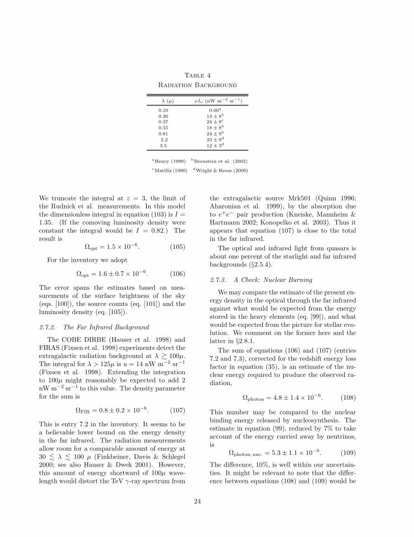
Table 4

Radiation Background

λ (µ) νIν (nW m−2 sr−1)

0.10 0.60a

0.30 13 ± 8b

0.37 24 ± 8c

0.55 18 ± 8b

0.81 24 ± 9b

2.2 23 ± 9d

3.5 12 ± 3d

aHenry (1999) bBernstein et al. (2002)

cMatilla (1990) dWright & Reese (2000)

We truncate the integral at z = 3, the limit ofthe Rudnick et al. measurements. In this modelthe dimensionless integral in equation (103) is I =1.35. (If the comoving luminosity density wereconstant the integral would be I = 0.82.) Theresult is

Ωopt = 1.5 × 10−6. (105)

For the inventory we adopt

Ωopt = 1.6 ± 0.7 × 10−6. (106)

The error spans the estimates based on mea-surements of the surface brightness of the sky(eqs. [100]), the source counts (eq. [101]) and theluminosity density (eq. [105]).

2.7.2. The Far Infrared Background

The COBE DIRBE (Hauser et al. 1998) andFIRAS (Fixsen et al. 1998) experiments detect theextragalactic radiation background at λ & 100µ.The integral for λ > 125µ is u = 14 nW m−2 sr−1

(Fixsen et al. 1998). Extending the integrationto 100µ might reasonably be expected to add 2nW m−2 sr−1 to this value. The density parameterfor the sum is

ΩFIR = 0.8 ± 0.2 × 10−6. (107)

This is entry 7.2 in the inventory. It seems to bea believable lower bound on the energy densityin the far infrared. The radiation measurementsallow room for a comparable amount of energy at30 . λ . 100 µ (Finkbeiner, Davis & Schlegel2000; see also Hauser & Dwek 2001). However,this amount of energy shortward of 100µ wave-length would distort the TeV γ-ray spectrum from

the extragalactic source Mrk501 (Quinn 1996;Aharonian et al. 1999), by the absorption dueto e+e− pair production (Kneiske, Mannheim &Hartmann 2002; Konopelko et al. 2003). Thus itappears that equation (107) is close to the totalin the far infrared.

The optical and infrared light from quasars isabout one percent of the starlight and far infraredbackgrounds (§2.5.4).

2.7.3. A Check: Nuclear Burning

We may compare the estimate of the present en-ergy density in the optical through the far infraredagainst what would be expected from the energystored in the heavy elements (eq. [99]), and whatwould be expected from the picture for stellar evo-lution. We comment on the former here and thelatter in §2.8.1.

The sum of equations (106) and (107) (entries7.2 and 7.3), corrected for the redshift energy lossfactor in equation (35), is an estimate of the nu-clear energy required to produce the observed ra-diation,

Ωphoton = 4.8 ± 1.4 × 10−6. (108)

This number may be compared to the nuclearbinding energy released by nucleosynthesis. Theestimate in equation (99), reduced by 7% to takeaccount of the energy carried away by neutrinos,is

Ωphoton,nuc. = 5.3 ± 1.1 × 10−6. (109)

The difference, 10%, is well within our uncertain-ties. It might be relevant to note that the differ-ence between equations (108) and (109) would be

24

increased if we adopted the estimate of the opticalbackground from source counts.

2.7.4. The X-ray — γ-Ray Background

Entry 7.4 in Table 1 is the integral of the radia-tion background spectrum compiled by Gruber etal. (1999) over the energy range 3 keV to 100 GeV.The largest contribution to the integral is at pho-ton energy ∼ 30 keV, but the convergence at highenergy is slow because the energy per logarithmicinterval of frequency varies about as νΩν ∼ ν−0.1.The measurement at 3 keV by De Luca & Molendi(2004) is about 1.3 times the Gruber et al. value.We have not attempted to adjust the entry for thismore recent result because we do not know its sig-nificance for the spectrum at higher energies.

2.7.5. The Radio Background

Longair (1995), following Bridle’s (1967) study,concludes that the brightness temperature of theisotropic radio background at 178 MHz, after cor-rection for the thermal component, is T = 27±7 K.This corresponds to

uν = 6600(1 ± 0.25)( ν

1GHz

)−0.8

Jy sr−1, (110)

assuming the canonical power law spectrum (seealso Peacock 1995). Longair also argues that thisradiation is dominated by galaxies.

Equation (110) may be compared to the sum ofthe radio source counts in the 9CR radio surveyat 15 GHz, in the observed range of flux densities,0.01 to 1 Jy (Waldram et al. 2003). This sum givesuν = 5900 Jy sr−1 when scaled to 1 GHz with thepower index of 0.8. The radio source counts at8.4 GHz by Fomalont et al. (2002), summed over10 µJy to 1 Jy, give uν = 4700 Jy sr−1 at 1 GHz.A comparable result is obtained from the countat 40 GHZ (as summarized in Figure 13 of Ben-nett et al. 2003b). Haarsma & Partridge (1998)argue that the integral over the counts likely con-verges at S ∼ 1µJy. We conclude that the mea-surements are reasonably concordant with equa-tion (110), within ∼0.2 dex.

The integral of equation (110) slowly divergesat short wavelengths. We adopt, as an operationaldefinition, a cutoff at λ = 1mm (ν = 300 GHz),and we count the contribution at shorter wave-lengths as part of the FIR background in our in-

ventory. There is a natural cutoff at long wave-length, at ν ∼3 MHz (Simon 1978). Integratingeq. (110) over this wavelength range, we obtain

Ωradio = 5 × 10−11. (111)

To understand the relation to other energy en-tries, we may attempt an alternative estimate bydirectly summing the contributions of known radiogalaxies. The luminosity function of radio galaxiesat zero redshift is now reasonably well known byvirtue of the correlation of a large NRAO VLA SkySurvey at 1.4 GHz (NVSS; Condon et al. 1998)with galaxies in optical catalogues (Condon, Cot-ton & Broderick 2002 [UGC vs. NVSS]; Machalski& Godlowski 2000 [LCRS vs. NVSS]; Sadler et al.2002 [2dF vs. NVSS]). The luminosity function iswritten as the sum of two components, weak radioemitters that represent normal galaxies with starforming activity, and strong emitters that mostlyconsist of subsets of giant elliptical galaxies andAGNs. The former activity is ascribed to electronacceleration in Type II (and Ib/c) supernova rem-nants. At close to zero redshift the integral overthe luminosity function gives luminosity densities

Lg = 1.5 × 1019W Hz−1 Mpc−3,

La = 3.7 × 1019 W Hz−1 Mpc−3, (112)

at 1.4 GHz (Condon et al. 2002). The second com-ponent, AGNs, is dominated by the most luminoussources, and so is subject to sampling fluctuations.Haarsma et al. (2000) show that the evolution ofthe first component in equation (112) is fast toz ∼ 1. The evolution they derive is consistentwith the model for the evolution of the star for-mation rate in equation (31). Condon (1992) givesthe relation between the radio emissivity and thestar formation rate. After adjustment for the over-all constraint from the star formation rate densityderived from the local Hα luminosity density, asdiscussed in §2.3.2, and our reference IMF, the re-lation reads

uν = 2.5 × 1021( ν

GHz

)−0.8

+2.6 × 1020( ν

GHz

)−0.1

W Hz−1, (113)

per 1 m⊙ yr−1 of star formation. The firstcomponent represents synchrotron radiation, pri-marily from supernovae, and the second rep-resents bremsstrahlung from HII regions. The

25

bremsstrahlung contribution becomes more im-portant above 25 GHz. The integral over the starformation history to zf = 3 (with the redshiftenergy loss) and the frequency range ν = 3 MHzto 300 GHz gives Ωradio = 3.3 × 10−11, wherethe contributions from synchrotron radiation andbremsstrahlung are in the proportion 0.4:0.6 inthe frequency range that concerns us.

The evolution of the strong radio sources ap-pears not to be very fast. The luminosity func-tions of Sadler et al. (2002) and Machalski &Godlowski (2000) up to z ∼ 0.2 suggest a slowevolution compared with that of the weak emit-ter component, at least at low redshifts. We takethe evolution factor derived from high redshiftstrong radio galaxies by Willott et al. (2001),(1 + z)2.6E(z) with E(z) = [Ωm(1 + z)3 + Ωλ]1/2,and we assume the canonical synchrotron spec-trum. The integral over time and frequency yieldsΩradio = 2.0 × 10−11. The sum of the two compo-nents is

Ωradio = 5 × 10−11. (114)

The consistency with equation (111) suggests thatthis simple model for the radio sources is a usefulapproximation.

2.7.6. Gravitational Radiation

We consider two sources of gravitational radia-tion, the merging of stellar mass binaries and theformation of massive black holes in the centers ofgalaxies. The rate of production of gravitationalradiation by stellar mass binaries in the MilkyWay depends on the very uncertain distributionof properties of close binary systems that containwhite dwarfs, neutron stars, and black holes. Thelargest contribution to the mean gravitational ra-diation luminosity of the Milky Way is thought tobe from the merging of binary neutron stars, asindicated in Fig. 12 in Schneider et al. (2001).

Shibata & Uryu (2002) and Faber et al. (2002)find that in the merging of a binary neutron starsystem the energy emitted as gravitational radia-tion is

ǫGWnn ≃ 0.005 (115)

times the mass of the binary. A major uncertaintyis the behavior of the system after contact. Gravi-tational radiation emitted during the transient for-mation of an oscillating neutron star might doublethe number in equation (115).

If we adopt the estimate of the rate of merg-ing of binary neutron stars in the Milky Way,R ≈ 80 Myr−1, that is based on the three knownsystems that will merge within the Hubble time(Kalogera et al. 2004a, b), then we find thatthe product with the radiation energy released(eq. [115]), the effective number density of MilkyWay galaxies (eq. [54]), and 85 Gyr/2 (eqs. [35]and [36]) is the gravitational radiation energy den-sity ΩNS,gw = 10−9. The merger rate is higly un-certain: the spread of central values in the modelsin Table 1 in Kalogera et al. (2004b) is 10+0.7

−1 .On taking account of the upward uncertainty inequation (115), we are led to allocate an error ofa full order of magnitude up or down in entry 7.5.

The merging rates for neutron star-black holeand black hole-black hole binaries are even moreuncertain. The indication from the analysis ofSchneider et al. (2001) is that mergers involvingblack holes add about 10% to the gravitational ra-diation luminosity.

In the low frequency regime (∼ mHz) the lu-minosity is dominated by compact white dwarfbinaries, as shown by Hils, Bender & Webbink(1990). The integration of the gravitational lu-miosity given in their Table 7 with the number ofclose white dwarf binaries in the Milky Way nor-malised to 3× 106 (after a suggested reduction bya factor of ten from the simple theoretical estimateof the abundance of these objects) gives the lumi-nosity 3 × 1039 erg s−1. The product with theeffective number density of Milky Way galaxiesand the effective time span with redshift correc-tion gives ΩWD,gw ∼ 10−10. This is at the lowerend of the suggested range of uncertainty in thevalue of ΩNS,gw.

Our estimate of the gravitational radiation re-leased by the formation of the massive black holesin the centers of galaxies is based on the analy-sis by Baker et al. (2001), which indicates thatthe gravitational radiation energy released by themerging of equal mass black holes is ǫngw ≃ 0.03times the final black hole mass M , and thatthe frequency of the radiation is on the order of0.1M−1, or about 10−4M9 Hz when the mass ismeasured in units of 109m⊙. We take the redshiftat peak production to be zn ∼ 2.5, about the peakof quasar activity. Then the present energy den-sity of the gravitational radiation from the forma-tion of the massive black holes, with mass density

26

Ωn = 10−5.4, is Ωngw ∼ ǫngwΩn/(1+zn) ∼ 10−7.5.This may be compared to the bound on the grav-itational wave energy density from pulsar timingmeasurements, Ωg < 10−8 at frequency ∼ 10−8 Hz(Kaspi, Taylor & Ryba 1994; Thorsett & Dewey1996; Lommen & Backer 2001). The bound isabout 30% of our estimate of Ωngw, but there isno inconsistency because the expected peak fre-quency is considerably larger than the frequencywhere the pulsar constraint is tight. The spec-trum of the gravitational radiation from mergingmassive black holes, and the puzzle of how merg-ing black holes get close enough that energy lossby gravitational radiation drives merging withina Hubble time, are discussed by Hughes et al.(2001), Jaffe & Backer (2003) and Wyithe & Loeb(2003).

An entry in the inventory for possible sources oflow frequency gravitational radiation in the earlyuniverse, as from inflation or phase transitions,seems premature.

2.8. Products of Stellar Evolution

It is in principle straightforward to compute theintegrated outputs of stellar evolution — energy,neutrinos, helium, and heavy elements — givenmodels for the IMF, the star formation history,and stellar evolution. Since the details of the re-sults of stellar evolution computations are not eas-ily assembled, we use approximate estimates byprocedures similar to those developed in §2.3.1 and2.3.2 for the stellar population and its evolution.The results add to the checks of consistency ofour estimates of the stellar production of heliumand heavy elements and the resulting total energyrelease, and are used to estimate the inventory en-tries for the neutrino cosmic energy density.

2.8.1. Stellar Evolution

Most stars with masses m < 1m⊙ are stillon the main sequence. We assume that on av-erage 5% of the hydrogen in these subsolar starshas been consumed, with energy production ef-ficiency 0.0071. Most of the stars with massesm > 1m⊙ have already undergone full evolu-tion and left compact remnants, while the fraction∼ (m/m⊙)−2.5 is still on the main sequence. Weassume that in the latter stars on average 5% ofthe hydrogen has been consumed, as for subsolar

stars. For the evolved stars we do not attemptto follow the details of nuclear burning and massloss. Instead, we adopt estimates of the nuclearfuel consumed or mass lost in a few discrete stagesof evolution, in a similar fashion to the approachused in §2.3.1 to tally stellar remnants.

When the amount of hydrogen consumed instellar burning is 10% of the mass of a star it leavesthe main sequence. In the model in §2.3.1, starswith masses in the range 1 < m < 8m⊙ eventu-ally produce white dwarfs that mainly consist ofa carbon-oxygen core. In standard stellar evolu-tion models, hydrogen burning extends outwardto a shell after core hydrogen exhaustion, and he-lium burning similarly continues in a shell aftercore helium exhaustion. That leaves a CO corewith the mass given by equation (69). The heliumlayer outside the CO core is thin for m < 2.2m⊙,for which helium ignition takes place as a flash,but in stars with masses m > 2.2m⊙ a signif-icant amount of helium is produced outside thecore, transported by convection to the envelope,and liberated. A 5m⊙ star liberates 0.4m⊙ of he-lium and produces a core with mass 0.85m⊙ (e.g.,Kippenhahn, Thomas & Weigert 1965). We modelthe helium production as a function of the initialstar mass m as

mHe = 0.23(m− 2.2) + 0.63, (116)

in solar mass units. The energy production in hy-drogen shell burning is the product of this masswith the post-stellar hydrogen mass fraction, 0.71(eq. [87]), and the efficiency factor, 0.0071. Heliumburning in the core produces energy with efficiencyfactor 0.0010.

For stars with masses m > 8m⊙ we adopt thehelium yield from Table 14.6 of Arnett (1996),15

which we parametrise as

mHe = 0.69m− 3.9. (117)

This connects to equation (116) at 8.7m⊙. Wetake the CO core mass as a function of the initialstellar mass from Arnett (1996):

mCO = 0.28m− 2.20, m > 13m⊙. (118)

We use an interpolation of eqs. [69] and [118] forstellar masses between 8 and 13m⊙. The energy

15We prefer eq.[117] which is derived from tabulated values,rather than Arnett’s parametrisation, mHe = 0.43m−2.46.

27

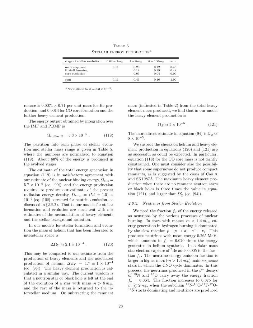
Table 5

Stellar energy productiona

stage of stellar evolution 0.08 − 1m⊙ 1 − 8m⊙ 8 − 100m⊙ sum

main sequence 0.11 0.20 0.12 0.43H shell burning 0.18 0.29 0.48core evolution 0.05 0.04 0.09

sum 0.11 0.43 0.46 1.00

aNormalised to Ω = 5.3 × 10−6.

release is 0.0071 × 0.71 per unit mass for He pro-duction, and 0.0014 for CO core formation and thefurther heavy element production.

The energy output obtained by integration overthe IMF and PDMF is

Ωstellar E = 5.3 × 10−6 . (119)

The partition into each phase of stellar evolu-tion and stellar mass range is given in Table 5,where the numbers are normalised to equation(119). About 60% of the energy is produced inthe evolved stages.

The estimate of the total energy generation inequation (119) is in satisfactory agreement withour estimate of the nuclear binding energy, ΩBE =5.7 × 10−6 (eq. [99]), and the energy productionrequired to produce our estimate of the presentradiation energy density, Ωγ+ν = (5.1 ± 1.5) ×10−6 (eq. [108] corrected for neutrino emission, asdiscussed in §2.8.2). That is, our models for stellarformation and evolution are consistent with ourestimates of the accumulation of heavy elementsand the stellar background radiation.

In our models for stellar formation and evolu-tion the mass of helium that has been liberated tointerstellar space is

∆ΩY ≈ 2.1 × 10−4 . (120)

This may be compared to our estimate from theproduction of heavy elements and the associatedproduction of helium, ∆ΩY = 1.7 ± 1 × 10−4

(eq. [96]). The heavy element production is cal-culated in a similar way. The current wisdom isthat a neutron star or black hole is left at the endof the evolution of a star with mass m > 8m⊙,and the rest of the mass is returned to the in-terstellar medium. On subtracting the remnant

mass (indicated in Table 2) from the total heavyelement mass produced, we find that in our modelthe heavy element production is

ΩZ ≈ 5 × 10−5 . (121)

The more direct estimate in equation (94) is Ω′Z ≃

8 × 10−5.

We suspect the checks on helium and heavy ele-ment production in equations (120) and (121) areas successful as could be expected. In particular,equation (118) for the CO core mass is not tightlyconstrained. One must consider also the possibil-ity that some supernovae do not produce compactremnants, as is suggested by the cases of Cas Aand SN1987A. The maximum heavy element pro-duction when there are no remnant neutron starsor black holes is three times the value in equa-tion (121), and larger than Ω′

Z (eq. [94]).

2.8.2. Neutrinos from Stellar Evolution

We need the fraction fν of the energy releasedas neutrinos by the various processes of nuclearburning. In stars with masses m < 1.4m⊙, en-ergy generation in hydrogen burning is dominatedby the slow reaction p + p → d + e+ + νe. Thisproduces neutrinos with mean energy 0.265 MeV,which amounts to fν = 0.020 times the energygenerated in helium synthesis. In a Solar massstar electron capture of 7Be adds 0.005 to the frac-tion fν . The neutrino energy emission fraction islarger in higher mass (m > 1.4m⊙) main-sequencestars in which the CNO cycle dominates. In thisprocess, the neutrinos produced in the β+ decaysof 13N and 15O carry away the energy fractionfν = 0.064. The fraction increases to 0.075 form & 2m⊙, when the subchain 15N-16O-17F-17O-14N starts dominating and neutrinos are produced

28

by the beta decay of 17F. This sidechain also dom-inates during shell burning.

The integral of these factors over the stellarIMF normalised to the present-day mass densityΩstar = 0.0027 (eq. [27]), together with our pre-scription for energy generation in Table 5, yieldsthe neutrino energy production,

Ων,ms = 0.31 × 10−6. (122)

The temperatures and densities that are reachedup to carbon burning are low enough that there isnegligible neutrino energy loss from neutrino pairproduction processes.

The temperatures after carbon burning are highenough that the neutrino energy loss dominates,that is, fν ≃ 1 (Weaver et al. 1978). Thus wemay take it that the extra binding energy ∆(BE)of the elements heavier than 20Ne with respectto the binding energy of carbon represents theneutrino energy emitted in the late stages of stel-lar evolution. On multiplying the heavy elementmass (the sum of entries 1, 2 and 4 to 9 in Table3) by

∑

(Zi/Z)∆(BE)i (where 〈∆(BE)〉 = 0.0004for the solar mix of element abundances, and∑

Zi/Z = 0.35 is from Grevesse & Sauval (2000),we obtain

Ων,pairs = 0.03 × 10−6. (123)

The sum of equations (122) and (123) is 7%of the total energy production (eq. [119]). Thepresent energy density of the stellar neutrinos, inentry 8.1 in Table 1, is the product of this sumwith the redshift loss factor ∼ 0.5 (eq. [35]).

2.8.3. White Dwarfs and Neutron Stars

Most of the gravitational energy liberated inwhite dwarf formation goes to neutrinos, and inthe latest stage to X-rays. Since the latter is smallthe contribution to the neutrino energy density(entry 8.2 in the inventory) is the product of thegravitational binding energy in entry 5.3 with theredshift factor.

More than 99% of the energy released in corecollapse also is carried away by neutrinos. Thuswe similarly obtain entry 8.3 by multiplying entry5.4 by the redshift factor.

2.9. Cosmic Rays and Magnetic Fields

This estimate is based on the rate of productionof cosmic rays in the Milky Way galaxy. We startfrom the radio structure. In their analysis of theHaslam et al. (1982) measurements, Beuermann,Kanbach, & Berkhuijsen (1985) write the radioluminosity distribution at 408 MHz as the sumof thin and thick components. We model eachdistribution, in an approximation to their results,as

E(~r) = E(0)e−(|z|/zeq+r/l). (124)

In the thick component the scale heights in thedisk and perpendicular to the disk are

l = 3.1 kpc, zeq = 1.4 kpc, (125)

scaled to Solar galactocentric distance 8 kpc (seeAppendix). The total luminosity in the thin com-ponent in this model may be neglected, but thethin component is a significant contribution to thelocal luminosity density, E⊙: the local thick com-ponent fraction is E⊙(thick)/E⊙ = 0.55. We as-sume the energy density in cosmic rays is propor-tional to the luminosity density at 408 MHz. Amore detailed model would take account of thespatial variation of the magnetic field strength,but that will be left for future studies. We nor-malize to the local energy density, 1.8 eV cm−3,in relativistic cosmic rays (Webber 1998). In theseapproximations the energy of cosmic rays in thegalaxy is 1056.1 erg. We take the cosmic ray meanlife in the galaxy to be 2× 107 yr (Garcia-Munoz,Mason & Simpson 1977; Yanasak et al. 2001).The ratio is a measure of the cosmic ray luminos-ity, 1041.3 erg s−1. If the acceleration of cosmicrays is mainly due to shocks of Type II and Ibcsupernovae,16 following the conventional wisdom(Ginzburg & Syrovatskii 1964), the cosmic ray lu-minosity is proportional to the star formation rate.Thus the product of this luminosity with the effec-tive time (eq. 36) and the redshift factor (eq. [35])is an estimate of the contribution of the Milky Wayto the present energy in cosmic rays. The productwith the effective number density of Milky Waygalaxies (eq. [54]) is our estimate of the present

16No type Ia supernova remnants are known to give strongradio sources (Weiler et al. 1986). This implies that TypeIa supernovae contribute little to the acceleration of cosmicrays.

29

energy density in cosmic rays from normal galax-ies,

ΩCR = 10−8.3. (126)

The radio luminosity of the Milky Way offersa check of this calculation. The Beuermann et al.(1985) luminosity of the Milky Way, 5.5 × 1021

W Hz−1 at ν = 408 GHz, scaled to 1.4 GHz bythe ν−0.8 power law (neglecting the small thermalbremsstrahlung component), and multiplied bythe effective number density of Milky Way galaxies(eq. [54]), is Lg = 9× 1018 W Hz−1 Mpc−3, abouthalf the Condon et al. (2002) measurement of themean luminosity density of the galaxies (eq. [112]).That is, the evidence is that the Milky Way givesa reasonably good measure of the synchrotron lu-minosity density of the galaxies, and hence of thecosmic ray luminosities of galaxies. This is not avery direct check of the assumed universality of thecosmic ray lifetime in the source galaxy, of course.

A similar energy may be present in the mag-netic field. If the leakage of cosmic rays approxi-mated a fluid flow, magnetic field would leak intointergalactic space with the cosmic rays. Applica-tion of equipartition to equation (126) would sug-gest that the cosmic rms magnetic field strengthis

BIGM ∼ 3 × 10−8 Gauß. (127)

If the estimate of the local ratio of the cosmic rayto magnetic field energy density, 8:1 (the magneticfield corresponding to 3 µGauß), applied to the in-tergalactic medium, it would lower equation (127)by a factor of three.

The product of the integrated production ofsupernovae with the characteristic kinetic energy,EKE ≃ 1.6×1051 erg, released in a supernova (Ar-nett 1996), is an estimate of the integrated kineticenergy production per comoving volume,

ΩSN KE ≃ 10−7.3. (128)

If the fraction ǫcr of this energy were placed in rel-ativistic intergalactic particles, the present energydensity in this component, taking account of theredshift factor, would be

ΩSN cr ≃ 10−7.6ǫcr. (129)

This is consistent with the picture that a frac-tion ǫcr ∼ 0.2 of the kinetic energy liberatedby supernovae has been deposited in cosmic rays(eq. [126]), which eventually become intergalactic.

Cosmic rays might gain energy from shocks pro-duced by streaming motions of magnetized warmplasma in the vicinity of galaxies (Loeb & Wax-man 2000). However, since the energy available inthe plasma (eq. [130] below) is less than the energyliberated by supernovae (eq. [126]), this process isnot likely to substantially affect the energy in cos-mic rays.

What is the AGN contribution to the cosmicray energy density? Though AGNs are not majorsources at optical wavelengths, their contributionto the radio background is comparable to that ofthe larger number of normal galaxies (eq. [112).This is an indication of the importance of AGNsfor high energy processes. If the cosmic ray energyproduction by AGNs were proportional to the pro-duction of synchrotron radio emission, the energyof cosmic rays from AGN’s (including radio ellip-tical galaxies) would be comparable to, or evenlarger than, that from the normal galaxies, andour estimate in eq. (126) would have to be dou-bled. It is important also that AGNs may acceler-ate cosmic rays to higher energies than do normalgalaxies.

We use equation (126) in the inventory. Thelower error flag for the entry in Table 1 is based onthe evidence that the Milky Way gives a fair mea-sure of galaxy radio luminosities. The larger uppererror flag reflects the possibly significant roles ofthe intergalactic magnetic field and AGNs.

2.10. Kinetic Energy in the IGM

Intergalactic baryons have peculiar velocitiesthat are driven by the gravitational field of thedark matter distribution and by nongravitationalinteractions. The former is part of the primevalenergy in category 4 in the inventory. The latter isexpected to be most important near the virializedregions of galaxies, where the streaming motionhas been largely transformed by shocks into ther-mal energy at the temperature T ∼ 2 × 106 Kassociated with the nominal velocity dispersionσ = 160 km s−1 around L ∼ L∗ galaxies (eq. [10]).This shocked matter may be responsible for theO VI absorption lines in the Local Group (Sem-bach et al. 2003; Cen et al. 2001). The productof the internal energy per unit mass of plasma atthis temperature with the mass fraction in entry3.1a is

ΩKE ≃ 10−8.0. (130)

30

If an appreciable fraction of the kinetic energyproduced by supernovae (eq. [128]) were depositedas kinetic energy in galactic haloes this energywould be dissipated by hydrodynamic processesrather than the cosmological redshift, but stillmay make a significant addition to equation (130),heating the IGM relative to dark matter.

Baryonic matter well outside the nominal viri-alized regions of galaxies and larger systems — atdistances greater than about r200 from clusters ofgalaxies and rv ∼ 200 kpc from L ∼ L∗ galaxies— is observed as Lyα absorption systems (Pen-ton, Stocke & Shull 2004). The primeval peculiarmotions of this matter are perturbed by photoion-isation that produces kinetic temperatures on theorder of 104 K. The product of this kinetic energyper unit mass with the intergalactic mass frac-tion (entry 3.1b) is about one percent of the ki-netic energy in the warm intergalactic component(eq. [130]).

We use equation (130) for category 10. Wecaution, however, that a comparable amount ofkinetic energy may be deposited by supernovawinds.

2.11. Electrostatic Energy

The effect of the electrostatic interaction on thebinding energies of atomic nuclei relative to freeprotons and electrons is taken into account in cat-egory 6, and the electrostatic contribution to thebinding energies of white dwarfs is (in principle)part of category 5. The molecular binding energyin objects ranging from dust to asteroids that areheld together by the electrostatic interaction de-serves separate mention.

The molecular binding energy relative to freeatoms in condensed matter is roughly 1 eV peratom. The product of this mass fraction, ∼ 10−10,with entry 3.12 is

ΩBE,molecular ∼ −10−16. (131)

This is the binding energy of condensed matterphysics outside strongly self-gravitating systems.We refrain from entering it in Table 1 because theestimate is so small and uncertain, but we offer forcomparison the binding energy of the electrons inatoms.

The electrostatic binding energy of the elec-trons in an O VI atom is 1.6 keV, and the ad-

dition of the other five electrons in a neutral oxy-gen atom increases the binding energy by only 27percent. That is, it is a reasonable approxima-tion to ignore the states of ionization of the heavyelements and the electrostatic binding energy ofneutral hydrogen and helium. The sum over theheavy element masses in entries 1, 2, 4, 5, and 6 inTable 3, weighted by the neutral atomic bindingenergies of 15 cosmically conspicuous elements, is

ΩBE,atoms = −10−9.7. (132)

This is some six orders of magnitude larger thanthe molecular binding energy in equation (131),and comparable in value to the smallest entries inTable 1.

3. Discussion

The convergence of the cosmological tests fromredundant constraints on the global cosmologi-cal parameters offers a good case for the ΛCDMFriedmann-Lemaıtre cosmology as a useful ap-proximation to the real world. This is a neces-sary condition that our compilation of the energyinventory is a meaningful exercise.

We adopt the working assumption that thegalaxies are useful tracers of mass, in the sensethat inventory entries derived under this assump-tion are good approximations to reality. This as-sumption has been widely questioned. However,the recent evidence from weak lensing (eqs. [3]to [7]), with the older evidence from the galaxy rel-ative velocity dispersion at separations ∼ 100 kpcto 1 Mpc, and the consistent picture for the viri-alized parts of field galaxies (eq. [10]), offer whatseems to be a reliable case for the use of galaxies asmass tracers. The approach certainly is not exact,and working out more accurate measures of themass distribution on the scale of galaxies remainsan important and fascinating challenge.

Our other conventions for the cosmology areless controversial but may have to be adjusted.For simplicity, we have adopted a fixed distancescale (eq. [1]). We have not presented the scalingof inventory entries with the distance scale, whichcan be somewhat complicated; this issue is best re-visited when the uncertainty in the distance scaleis better understood. Our adopted value and for-mal uncertainty for the matter density parameter,Ωm (eq. [8]), is in the generally accepted range, but

31

there is reason to suspect that it is somewhat over-estimated (§2.1). Again, this is a issue to revisitwhen the constraints have improved. Our valuefor the baryon mass density agrees with what isderived from the CMBR anisotropy and the mea-surements of the primeval deuterium abundance,but it is larger than what is indicated by theprimeval helium abundance. We have suggestedin §2.2.2 that the problem may be with the tech-nical difficulties of the helium measurements, butwe will be following the advances in this subjectwith interest. It would not be surprising to seethe discovery of richer physics in the dark sector,and with it an increase in the variety of entries incategory 1, and possibly also some adjustment ofother parts of the inventory that depend on thedark sector physics. One should also bear in mindthat the alternative pictures of structure forma-tion that were under discussion a decade ago, suchas cosmic strings, could be operating as subdomi-nant perturbations to the ΛCDM model. Furtherprogress in testing the model for structure forma-tion will inform our ideas on whether the entriesthat depend on the theory of structure formationare likely to require adjustment. Each of theseissues may be pointing to revisions to the inven-tory outside our stated errors. On the other hand,the successful network of tests of the cosmologyand the model for structure formation leads us toexpect that the general framework presented inTable 1 is not likely to change.

We have argued that 6± 1% of the baryons arein stars and stellar remnants (eqs. [17] and [27]with h = 0.7). This small fraction is analyzedin considerable detail in the inventory, in entriesthat are supported by a network of tests. The esti-mate in §2.7.1 of the mass density in stars uses theoptical luminosity density and the stellar-mass-to-light ratio. The luminosity density is checked bymeasurements of the optical to near infrared in-tergalactic radiation energy density, and by themeasured galaxy counts (§2.7.1). The comparisonis not tight, but it shows that the radiation energydensity likely is known to ±0.3 dex. The conver-sion from the luminosity density to the stellar massdensity depends on the model for the stellar initialmass function. The model we use is checked by thereasonable agreement with the ratio of the whitedwarf to subsolar main sequence star densities atthe low mass end, and with the global Type II su-

pernova rate at the high mass end (2.3.1, 2.3.2).The model for the star formation history is basedon the time history of the Hα luminosity density,which is broadly consistent with other measuresof the evolution of the star formation rate density(subject to the considerable uncertainty in extinc-tion in the UV). The model is checked by consis-tency with the accumulated mass in stars (aftercorrection for mass loss; eq. [34]). Yet anothercheck involves the accumulated mass density inheavy elements. The release of nuclear bindingenergy in the heavy elements, corrected for theloss of radiation energy by the cosmological red-shift (eq. [35]), is in satisfactory agreement withthe present radiation energy density at near op-tical and far infrared wavelengths (§2.7.3). Thistest would fail if there were a substantial amountof radiation energy at wavelengths 1µ < λ < 100µ;improved measurements will be of considerable in-terest. This test also depends on the stellar pro-duction of helium, which is discussed in §2.2.2, inconnection with the constraint on the baryon massdensity from the primeval helium abundance, andin §2.8.1, from an analysis of the products of stellarevolution. The results seem reasonably consistent.The network of checks is complicated, but that iswhat lends credence to the results.

It is well to pause to consider Arp’s (1965) cau-tionary remark, that there may be extragalacticobjects with sizes too small to be readily distin-guished from stars — an example is the quasi-stellar objects Arp mentions in a note added inproof — or with surface brightnesses too low tobe readily seen against the foreground — an ex-ample is the intracluster light in the Virgo clus-ter (Arp & Bertola 1971). The quasar remnantscould have contained a significant baryon mass, ifthe mass conversion efficiency ǫn had been closeto unity (eq. [73]), but we now know that thatis difficult to reconcile with the integrated quasarenergy emission (eq. [83]). There are low surfacebrightness objects (e.g McGaugh, Schombert, &Bothun 1995), but the surface brightness of theextragalactic sky shows that they cannot largelyaffect our estimate of the mean luminosity density(§2.7.1). Substellar objects might be counted aspart of Arp’s cautionary remark, but they are de-tectable in nearby galaxies by weak gravitationallensing (or MACHOs, as discussed by Alcock etal. 2000 and references therein). That is, a half

32

century ago it was not clear that it is feasible toestablish a fair observational census of the stars.Now it appears that the observational conditionsallow it: the closure of our inventory suggests thatmissing or unknown components cannot be ener-getically very significant.

The baryon number density — excludingbaryons that may have been sequestered prior tolight element production — seems to be reliablyconstrained, but the states of most of the baryonsare not yet observationally well documented. Thepicture that galaxies trace mass leads us to ex-pect that about half the dark matter is gatherednear and within the virialized parts of the galax-ies (eq. [13]). Entries 3.1 and 3.2 in Table 1 arebased on the assumption that the baryons are sim-ilarly placed, in the diffuse states observed as hotplasma in clusters of galaxies and in warm and hotplasma in and around groups of galaxies (eq. [56]).This has not yet been convincingly observation-ally demonstrated. We have not made much useof the predicted states of the baryons from numer-ical simulations, because we do not know how tojudge the reliability of the predictions on relativelysmall scales. As the computations and their obser-vational checks improve this will become clearer,and the results may be expected to improve thispart of the inventory.

The advances in observations of the massivecompact objects in the centers of galaxies allow animproved test of the idea that these objects are theblack hole remnants of quasars and AGNs that arepowered by gravitational accretion. Our estimatesof the mass density in black holes and the luminos-ity density in quasars require that the quasar massconversion efficiency is ǫn ∼ 0.02 (eq. [86]), close tothe efficiency of production of gravitational radi-ation (§2.7.6). If the estimate of the quasar lumi-nosity density has missed a significant populationof optically faint AGNs then our value of ǫn is bi-ased low. The quasar luminosity density is quiteuncertain, as is the actual value of ǫn, but it is en-couraging that the present result is as close as itis to conventional ideas about the quasar emissionmechanism.

The efficiency of conversion of mass into elec-tromagnetic radiation in the formation of stellarmass black holes is constrained to be less thana few percent by the observed energy density inelectromagnetic radiation and neutrinos. The in-

terpretation of this constraint awaits developmentof the theory of the astrophysical processes of for-mation of stellar mass black holes. Our estimate ofthe gravitational binding energy released by corecollapse supernovae (entry 8.3) is comparable tothe energy released in the formation of the mas-sive black hole quasar remnants, and it is not verymuch less than the upper bound from neutrinodetectors. Progress here will be followed with in-terest.

The largest energy densities in the inventoryare in dark matter and dark energy. Any em-pirical hints to the natures of these componentswill be followed with great interest. One possibil-ity is that the observations of microlensing towardthe Magellanic Clouds have detected massive com-pact dark objects (Alcock et al. 2000; Afonso etal. 2003). We have adopted the conservative in-terpretation, that the lenses are baryonic — starsand stellar remnants — with standard mass func-tions, and that the high lensing rate is an accidentof the distributions of source and lensing stars.A demonstration of the apparently simpler inter-pretation, that the lenses contribute some 20% ofthe mass of the halo of the Milky Way, and arebaryonic, perhaps white dwarfs, would consider-ably upset our considerations of the stellar baryonbudget; a demonstration that the lenses are non-baryonic would profoundly affect thinking aboutdark matter and the early universe.

Though there are large gaps in our understand-ing of the cosmic energy inventory, most notablyin the dark sector, there also is an impressivelybroad observational basis for many parts of theinventory. Ten years ago the basis was consider-ably smaller, and we can be sure that ten yearsfrom now the observations will allow more entriesand a richer network of crosschecks of the inter-pretations. Progress will be uneven, of course, asone sees by considering the prospects for furtherchecks of the neutrino energy inventory. With therecent demonstration that the solar neutrino lumi-nosity agrees with standard physics augmented byneutrino masses and mixing angles (Bahcall 2003and references herein) we may now be confidentthat the theory of neutrino production by stel-lar nuclear burning is reliably tested even in theabsence of a direct observation of stellar neutri-nos from remote stars. The neutrinos producedby plasma processes in white dwarf formation are,

33

while an enormous energy density, too soft for de-tection by any conceivable method: estimates ofthis component of the inventory will have to con-tinue to rely on the theory. Neutrinos released instellar core collapse have been detected (Hirata etal. 1987; Bionta et al. 1987), and the integratedbackground of relic neutrinos from this process isexpected to be within experimental reach. Thedetection would complete another valuable checkof the cosmic energy transactions.

Parts of our inventory can be improved on thebasis of what is available within existing compu-tations, or could be readily developed from exist-ing work, but that we could not readily assemble.In particular, the theoretical analyses of stellarremnants and the other products of stellar evo-lution (§§2.3.1 and 2.8), with special attention tothe white dwarfs that store so much of the heavyelements, will have to be done better. Anotherexample is the heavy element abundances, whichcan be classified by element type, as oxygen —which has a specific spectroscopic importance —and the α-elements and the iron group, and by en-vironment, as white dwarfs, main sequence stars,and interstellar and intergalactic space.

It is also worth stating explicitly that we mayexpect that, as in the past, there will be quali-tatively new experimental or observational devel-opments — perhaps the detection of gravitationalradiation, or the identification of dark matter par-ticles — that substantially affect the directions ofresearch and the development of the cosmic energyinventory.

4. Concluding Remarks

A half century ago we had a largely conjecturalpicture of the large-scale structure of the physi-cal universe, of its material contents, and of themain process that drive transformations amongthe states of matter and radiation. Now our worldpicture has a substantial basis in experiments andobservations and the attendant theories. This hasbeen an evolutionary process: none the entriesin the inventory in Table 1 requires a substantialdeparture from ideas that are under discussion,and in many cases have been in the literature fordecades. The important new development is thatwe now have observational support for the manyentries in Table 1, and a network of tests that

demonstrate that a considerable part of the in-ventory is a believable approximation. Continuedadvances in the observational and theoretical basisfor the inventory surely will yield unexpected re-visions and additions; we are attempting to drawlarge conclusions from limited observations of anexceedingly complex universe. However, the bigsurprise at the moment is that it is now possibleto find an inventory with observational support forthe largest ∼ 40 forms of energy.

We have benefited by advice from CharlesAlcock, Dave Arnett, John Bahcall, MichaelBlanton, Pierre Bergeron, Bruce Draine, DougFinkbeiner, Peter Goldreich, Andy Gould, VickyKalogera, Kim Griest, Craig Hogan, David Hogg,Guinevere Kauffmann, Julian Krolik, Jim Liebert,Geoff Marcy, Bruce Partridge, Martin Rees, NeillReid, Aldo Serenelli, Masaru Shibata, Mike Shull,Gary Steigman, Paul Steinhardt, Stuart Shapiro,Tomonori Totani, Scott Tremaine, Simon White,and the referee.

PJEP thanks the Japan Society for Promo-tion of Science for supporting his visit to Japan,where this work was initiated. MF received sup-port for this work from the Monell Foundation atthe Princeton Institute for Advanced Study, anda Grant in Aid from the Japanese Ministry of Ed-ucation at the University of Tokyo.

34

A. A Few Astrophysical Quantities for the Milky Way

The current best value for the distance to the Galactic center is

R0 = 7.94 ± 0.42 kpc, (A1)

from measurements of the orbit — proper motion and redshift — of a star close to Sgr A* (Eisenhauer etal. 2003). The product of this distance with the measurement of the proper motion of Sgr A∗ by Reid &Brunthaler (2004) is 241 km s−1. This velocity corrected for the solar proper motion is our adopted valueof the circular speed of the Milky Way at the Solar circle,

Θ0 = 234 ± 13 km s−1. (A2)

Traditionally, one invokes the Oort model to infer the circular speed, but Olling & Dehnen (2003) find thatthe current best result depends substantially on the stellar populations used in the analysis.

The circular velocity yields an estimate of the optical luminosity of the Milky Way via the Tully-Fisherrelation. To convert the optically measured maximum rotation velocity Vrot to the 20% line width of HImeasurements W20, we use the relation

W20/2 = (0.93 ± 0.02)Vrot + (27 ± 1.5)km s−1. (A3)

derived from the data given by Mathewson & Ford (1996). From the Galactic rotation curve from HI and COterminal velocities (using Fig. 9.17 of Binney & Merrifield 1998), we estimate that the maximum rotationvelocity of the Milky Way is Vmax = 1.03Θ0 = 241 ± 13 km s−1. Identifying Vmax = Vrot, we find

W20(MW) = 502 ± 30 km s−1. (A4)

From the COBE-DIRBE integrated light for the Milky Way in the near infrared (J, K, L) wavelengthbands, Malhotra et al. (1996) showed that the Milky Way is on the standard Tully-Fisher relation in thesewave length bands, slightly on the brighter side but within the dispersion around the relation. Assumingthat the Milky Way has the standard color of spiral galaxies, we may expect that the luminosity in the Bband also satisfies the Tully-Fisher relation for the B band. Using the Sakai et al. (2000) local calibration,

MBcT

= −19.80 − 7.97(logW20 − 2.5), (A5)

we findLBc(MW) = 1010.74±0.19L⊙, (A6)

where we use B⊙ = 5.46, and the error is dominated by the intrinsic dispersion (0.43 mag) of the B-bandTully-Fisher relation. The superscript c stands for extinction-free quantities.

An alternative estimate of the B-band luminosity uses the colour transformation applied to the DIRBEintegrated K-band luminosity of the Milky Way. A comparison of the samples of Malhotra et al.(1996) andSakai et al. (2000) indicates Bc

T −Kc = 2.84±0.10 for typical Sbc galaxies. Thus Kc(MW) = −23.95±0.25yields Bc

T= −21.1 ± 0.3, or

LBc(MW) = 1010.63±0.13L⊙. (A7)

Combining the two, our recommended value is

LBc(MW) = 4.6 ± 1.4 × 1010L⊙. (A8)

A value often quoted in the literature, LcB = 2.3 ± 0.6 × 1010L⊙ (van den Bergh 1988), is 1.5 standard

deviations below equation (A8).

The luminosity obtained here is the extinction-free value. When it is compared with L∗ that appears inthe luminosity function, we must take account of internal extinction. For consistency we use the average

35

value of the internal extinction correction in the Sakai et al. (2000) local calibration, AintB = 0.44 mag, or

an attenuation factor 1.5. This means that LB(MW) = 1.40L∗B at h = 0.7, and that the effective number

density of Milky Way galaxies is the value in equation (54), LB/LB(MW) = 0.013h3 Mpc−3.

36

REFERENCES

Abazajian, K., et al. 2003, AJ, 126, 2081

Afonso, C. et al. 2003, A&A, 400, 951

Aharonian, F. A., et al. 1999, A&A, 349, 11

Alcock, C. et al. (The MACHO Collaboration)2000, ApJ, 542, 281

Allende Prieto, C., Lambert, D. L., & Asplund,M. 2001, ApJ, 556, L63

Arnett, D. 1996, Supernovae and Nucleosynthe-sis: An Investigation of the History of Matter,from the Big Bang to the Present (Princeton:Princeton University Press)

Arp, H. 1965, ApJ, 142, 402

Arp, H. & Bertola, F. 1971, ApJ, 163, 195

Bahcall, J. N. 2003, astro-ph/0310030

Bahcall, J. N. & Pena-Garay, C. 2003, JHEP 0311,004

Bahcall, J. N. & Pinsonneault, M. H. 2004, Phys.Rev. Lett. 92, 12130

Bahcall, J. N., Pinsonneault, M. H., & Basu, S.2001, ApJ, 555, 990 (BP2000)

Bahcall, N. A. & Bode, P. 2003, ApJ, 588, L1

Bahcall, N. A. & Cen, R. 1993, ApJ, 407, L49

Bahcall, N. A., Lubin, L. M., & Dorman, V. 1995,ApJ, 447, L8

Bahcall, N. A., et al. 2003, ApJ, 585, 182

Baker, J., Brugmann, B., Campanelli, M. Lousto,C. O. & Takahashi, R. 2001, Phys. Rev. Lett.87, 121103

Basu, B. & Lynden-Bell, D. 1990, QJRAS, 31, 359

Bennett, C. L. et al. 2003a, ApJS, 148, 1

Bennett, C. L., et al. 2003b, ApJS, 148, 97

Bernstein, R. A., Freedman, W. L., & Madore,B. F. 2002, ApJ, 571, 56

Beuermann, K., Kanbach, G., & Berkhuijsen,E. M. 1985, A&A, 153, 17

Binney , J. & Merrifield, M. 1998, GalacticAstronomy (Princeton: Princeton UniversityPress)

Bionta, R. M., Blewitt, G., Bratton, C. B.,Caspere, D., & Ciocio, A. 1987, Physical Re-view Letters, 58, 1494

Blanton, M. R., et al. 2003, ApJ, 592, 819

Bosma, A. 1981, AJ, 86, 1825

Branch, D. 1992, ApJ, 392, 35

Bridle, A. H. 1967, MNRAS, 136, 219

Bruzual, G. & Charlot, S. 2003, MNRAS, 344,1000

Burgasser, A. J., Kirkpatrick, J. D., McElwain,M. W., Cutri, R. M., & Skrutskie, M. F. 2003,AJ, 125, 850

Burgasser, A. J., McElwain, M. W., Kirkpatrick,J. D., Cruz, K. L., Tinney, C. G., & Reid, I. N.2004, AJ, 127, 2856

Burrows, A. 1990, in Supernovae, ed. by Petschek,A. G. (Berlin: Springer), 143

Burrows, A., Hubbard, W. B., Lunine, J. I., &Liebert, J. 2001, Reviews of Modern Physics,73, 719

Calura, F. & Matteucci, F. 2004, MNRAS, 350,351

Cappellaro, E., Evans, R., & Turatto, M. 1999,A&A, 351, 459

Cappellaro, E., Turatto, M., Tsvetkov, D. Y., Bar-tunov, O. S., Pollas, C., Evans, R., & Hamuy,M. 1997, A&A, 322, 431

Cen, R., Tripp, T. M., Ostriker, J. P., & Jenkins,E. B. 2001, ApJ, 559, L5

Chabrier, G. 2003, PASP, 115, 763

Chen, H., Lanzetta, K. M., Webb, J. K., & Bar-cons, X. 2001, ApJ, 559, 654

Chiosi, C., Bertelli, G., & Bressan, A. 1992,ARA&A, 30, 235

Chokshi, A. & Turner, E. L. 1992, MNRAS, 259,421

37

Churchill, C. W., Vogt, S. S., & Charlton, J. C.2003, AJ, 125, 98

Claver, C. F., Liebert, J., Bergeron, P., & Koester,D. 2001, ApJ, 563, 987

Cole, S. et al. 2001, MNRAS, 326, 255

Colless, M., et al. 2001, MNRAS, 328, 1039

Condon, J. J. 1992, ARA&A, 30, 575

Condon, J. J., Cotton, W. D., & Broderick, J. J.2002, AJ, 124, 675

Condon, J. J., Cotton, W. D., Greisen, E. W., Yin,Q. F., Perley, R. A., Taylor, G. B., & Broderick,J. J. 1998, AJ, 115, 1693

Cox, A. N. (ed) 2000, Allen’s Astrophysical Quan-tities, 4th ed. (Berlin: Springer)

Cox, J. P. & Giulli, R. T. 1968, Principles of Stel-lar Structure, Vol. 2 (New York: Gordon andBreach)

Croom, S. M., Smith, R. J., Boyle, B. J., Shanks,T., Miller, L & Outram 2004, astro-ph/0403040

Davis, M. & Peebles, P. J. E. 1983, ApJ, 267, 465

De Luca, A. & Molendi, S. 2004, A&A, 419, 837

de Sitter, W. 1917, MNRAS, 78, 3

de Vaucouleurs, G. & Olson, D. W. 1982, ApJ,256, 346

Draine, B. T. 2003, ARA&A, 41, 241

Eguchi, K. et al. 2003, Phys. Rev. Lett. 90, 021802

Einstein, A. 1917, Sitzungsber Preuß Akad Wiss,p. 142 [English translation in The Principle of

Relativity (Dover, New York, 1952), p. 177]

Eisenhauer, F., Schodel, R., Genzel, R., Ott, T.,Tecza, M., Abuter, R., Eckart, A., & Alexan-der, T. 2003, ApJ, 597, L121

Elvis, M., et al. 1994, ApJS, 95, 1

Ezer, D. & Cameron, A. G. W. 1967, CanadianJournal of Physics, 45, 3429

Faber, J. A., Grandclement, P., Rasio, F. A., &Taniguchi, K. 2002, Physical Review Letters,89, 231102

Fan, X., et al. 2001, AJ, 121, 54

Fang, T., Marshall, H. L., Lee, J. C., Davis, D. S.& Canizares, C. R. 2002, ApJ, 572, L127

Fang, T., Sembach, K. R., & Canizares, C. R.2003, ApJ, 586, L49

Ferrarese, L. 2002, Proceedings, Second KIAS As-trophysics Workshop, Seoul, 2001, September3-7, Singapore: World Scientific, edited by Lee,C.-H., 3

Finkbeiner, D. P., Davis, M., & Schlegel, D. J.2000, ApJ, 544, 81

Fixsen, D. J., Cheng, E. S., Gales, J. M., Mather,J. C., Shafer, R. A., & Wright, E. L. 1996, ApJ,473, 576

Fixsen, D. J., Dwek, E., Mather, J. C., Bennett,C. L., & Shafer, R. A. 1998, ApJ, 508, 123

Fomalont, E. B., Kellermann, K. I., Partridge,R. B., Windhorst, R. A., & Richards, E. A.2002, AJ, 123, 2402

Freedman, W. L., et al. 2001, ApJ, 553, 47

Fukazawa, Y., Makishima, K., Tamura, T., Ezawa,H., Xu, H., Ikebe, Y., Kikuchi, K., & Ohashi,T. 1998, PASJ, 50, 187

Fukuda, Y., et al. 1998, Physical Review Letters,81, 1562

Fukugita, M. 2001, NATO ASIC Proc. 565: Struc-ture Formation in the Universe, 93

Fukugita, M., Hogan, C. J., & Peebles, P. J. E.1998, ApJ, 503, 518 (FHP)

Fukugita, M. & Kawasaki, M. 2003, MNRAS, 340,L7

Gallego, J., Zamorano, J., Aragon-Salamanca, A.,& Rego, M. 1995, ApJ, 455, L1

Gal-Yam, A. & Maoz, D. 2004, MNRAS, 347, 942

Gao, L., Loeb, A., Peebles, P. J. E., White, S. D.M. & Jenkins, A. 2003, astro-ph/0312499

Garcia-Munoz, M., Mason, G. M., & Simpson,J. A. 1977, ApJ, 217, 859

38

Ginzburg, V. I. & Syrovatskii, S. I. 1964, The Ori-gin of Cosmic Rays (Oxford: Pergamon)

Glazebrook, K., Blake, C., Economou, F., Lilly,S., & Colless, M. 1999, MNRAS, 306, 843

Glazebrook, K., et al. 2003, ApJ, 587, 55

Gott, J. R., Schramm, D. N., Tinsley, B. M., &Gunn, J. E. 1974, ApJ, 194, 543

Gebhardt, K., et al. 2000, ApJ, 539, L13

Gould, A., Bahcall, J. N., & Flynn, C. 1996, ApJ,465, 759

Grevesse, N. & Sauval, A. J. 2000, Origin of Ele-ments in the Solar System, Implications of Post-1957 Observations, Proceedings of the Interna-tional Symposium. ed. O. Manuel. (Dordrecht:Kluwer Academic Publishers), 261

Gruber, D. E., Matteson, J. L., Peterson, L. E., &Jung, G. V. 1999, ApJ, 520, 124

Gush, H. P., Halpern, M., & Wishnow, E. H. 1990,Physical Review Letters, 65, 537

Haarsma, D. B. & Partridge, R. B. 1998, ApJ, 503,L5

Haarsma, D. B., Partridge, R. B., Windhorst,R. A., & Richards, E. A. 2000, ApJ, 544, 641

Harris, H. C., et al. 2003, AJ, 126, 1023

Haslam, C. G. T., Stoffel, H., Salter, C. J., & Wil-son, W. E. 1982, A&AS, 47, 1

Hauser, M. G. & Dwek, E. 2001, ARA&A, 39, 249

Hauser, M. G., et al. 1998, ApJ, 508, 25

Hawkins, E. et al. 2003, MNRAS 346, 78

Hayashi, C., & Nakano, T. 1963, Prog. Theor.Phys. 30, 460

Heavens, A., Panter, B., Jimenez, R., & Dunlop,J. 2004, Nature, 428, 625

Heger, A., Woosley, S. E., Fryer, C. L., & Langer,N. 2003, From Twilight to Highlight: ThePhysics of Supernovae, 3 (astro-ph/0211062)

Henry, R. C. 1999, ApJ, 516, L49

Hils, D., Bender, P. L., & Webbink, R. F. 1990,ApJ, 360, 75

Hirata, K., Kajita, T., Koshiba, M., Nakahata,M., & Oyama, Y. 1987, Physical Review Let-ters, 58, 1490

Hubble, E. P. 1929, Proc Nat Acad Sci, 15, 168

Hubble, E. P. 1934, ApJ, 79, 8

Hubble, E. P. 1936, The Realm of the Nebulae(New Haven: Yale University Press)

Huchra, J., Jarrett, T., Skrustkie, M., Cutri, R.,Schneider, S., Macri, L., Steining, R., & Mader,J. 2003, IAU Symposium, 216, 174

Hughes, S. A., Marka, S., Bender, P. L. & Hogan,C. J. 2001, in Proceedings of Snowmass 2001,APS/DPF/DPB Summer Study on the Futureof Particle Physics, eConf C010630: p402 (alsoastro-ph/0110349)

Irvine, W. M. 1961, Doctoral Dissertation, Har-vard University

Ivezic, Z., et al. 2000, AJ, 120, 963

Izotov, Y. I. & Thuan, T. X. 2004, ApJ, 602, 200

Jaffe, A. H. & Backer, D. C. 2003, ApJ, 583, 616

Janka, H.-T. & Hillebrandt, W. 1989, A&A, 224,49

Jimenez, R., Flynn, C., MacDonald, J., & Gibson,B. K. 2003, Science, 299, 1552

Kalogera, V., et al. 2004a, ApJ, 601, L179

Kalogera, V., et al. 2004b, astro-ph/0312101, v. 3

Kameda, J. et al. 2001, in Proc. InternationalCosmic Ray Conference, Hamburg 2001, ed.K.-H. Kampert, G. Heizelmann & C. Spiering(Katlenburg-Lindau: Copernicus Gesellschaft,2001) Vol. 3, 1057

Kaspi, V. M., Taylor, J. H., & Ryba, M. F. 1994,ApJ, 428, 713

Kauffmann, G. et al. 2003, MNRAS, 341, 33

Kennicutt, R. C. 1983, ApJ, 272, 54

Keres, D., Yun, M. S., & Young, J. S. 2003, ApJ,582, 659

39

Kippenhahn, R., Thomas, H. C., & Weigert, A.1965, Zeits. fur Astrophysik, 61, 241

Kirkman, D., Tytler, D., Suzuki, N., O’Meara,J. M., & Lubin, D. 2003, ApJS, 149, 1

Kneiske, T. M., Mannheim, K., & Hartmann,D. H. 2002, A&A, 386, 1

Kobulnicky, H. A. & Zaritsky, D. 1999, ApJ, 511,118

Kochanek, C. S. et al. 2001, ApJ, 560, 566

Konopelko, A., Mastichiadis, A., Kirk, J., deJager, O. C., & Stecker, F. W. 2003, ApJ, 597,851

Kormendy, J. & Richstone, D. 1995, ARA&A, 33,581

Kroupa, P. 2001, MNRAS, 322, 231

Kumar, S. S. 1963, ApJ, 137, 1121

LaRoque, S. J., et al. 2003, ApJ, 583, 559

Layzer, D. 1963, ApJ, 138, 174

Lilly, S. J., Le Fevre, O., Hammer, F., & Cramp-ton, D. 1996, ApJ, 460, L1

Loeb, A. & Waxman, E. 2000, Nature, 405, 156

Lommen, A. N. & Backer, D. C. 2001, BAAS, 33,1347

Longair, M. 1995, Proceedings of the Extragalac-tic Background Radiation meeting, Baltimore,1993 May 18-20, Space Telescope Science Insti-tute Symposium Series, meeting, ed. Calzetti,D., Livio, M., & Madau, P. (Cambridge: Cam-bridge University Press), 223

Machalski, J. & Godlowski, W. 2000, A&A, 360,463

Madau, P., della Valle, M., & Panagia, N. 1998,MNRAS, 297, L17

Madau, P., Ferguson, H. C., Dickinson, M. E.,Giavalisco, M., Steidel, C. C., & Fruchter, A.1996, MNRAS, 283, 1388

Madau, P. & Pozzetti, L. 2000, MNRAS, 312, L9

Malhotra, S., Spergel, D. N., Rhoads, J. E., & Li,J. 1996, ApJ, 473, 687

Marcy, G. W. & Butler, R. P. 2000, PASP, 112,137

Mather, J. C., et al. 1990, ApJ, 354, L37

Mather, J. C., Fixsen, D. J., Shafer, R. A., Mosier,C., & Wilkinson, D. T. 1999, ApJ, 512, 511

Mathewson, D. S. & Ford, V. L. 1996, ApJS, 107,97

Mattila, K. 1990, IAU Symp. 139: The Galacticand Extragalactic Background Radiation, 139,257

McGaugh, S. S., Schombert, J. M., & Bothun,G. D. 1995, AJ, 109, 2019

McKay, T. A. et al. 2001, astro-ph/0108013

Merritt, D. & Ferrarese, L. 2001, ApJ, 547, 140

Molster, F. J., Waters, L. B. F. M., Tielens,A. G. G. M., Koike, C., & Chihara, H. 2002,A&A, 382, 241

Mushotzky, R. F., Cowie, L. L., Barger, A. J., &Arnaud, K. A. 2000, Nature, 404, 459

Mushotzky, R. F. & Loewenstein, M. 1997, ApJ,481, L63

Nakamura, O., Fukugita, M., Brinkmann, J., &Schneider, D. P. 2004, AJ, 127, 2511

Nakamura, O., Fukugita, M., Yasuda, N., Love-day, J., Brinkmann, J., Schneider, D. P., Shi-masaku, K., & SubbaRao, M. 2003, AJ, 125,1682

Nice, D. J., Splaver, E. M., & Stairs, I. H. 2003,ASP Conf. Ser. 302: Radio Pulsars, 75

Nomoto, K. 1984, ApJ, 277, 791

Olling, R. P. & Dehnen, W. 2003, ApJ, 599, 275

Pagel, B. E. J. & Portinari, L. 1998, MNRAS, 298,747

Pain, R., et al. 2002, ApJ, 577, 120

Partridge, R. B. & Peebles, P. J. E. 1967, ApJ,148, 377

40

Peacock, J. A. 1995, Proceedings of the Extra-galactic Background Radiation meeting, Bal-timore, 1993 May 18-20, Space Telescope Sci-ence Institute Symposium Series, meeting, ed.by Calzetti, D., Livio, M., & Madau, P. (Cam-bridge: Cambridge University Press), 237

Peebles, P. J. E. 1986, Nature, 321, 27

Peebles, P. J. E. & Partridge, R. B. 1967, ApJ,148, 713

Peebles, P. J. & Ratra, B. 2003, Reviews of Mod-ern Physics, 75, 559

Peimbert, M., Peimbert, A., & Ruiz, M. T. 2000,ApJ, 541, 688

Penton, S. V., Stocke, J. T. & Shull, J. M. 2004,astro-ph/0401036

Quinn, J., et al. 1996, ApJ, 456, L83

Reid, I. N., Gizis, J. E., & Hawley, S. L. 2002, AJ,124, 2721

Reid, M. J. & Brunthaler, A. 2004, astro-ph/0408107

Reimers, D. & Koester, D. 1982, A&A, 116, 341

Reiprich, T. H. & Bohringer, H. 2002, ApJ, 567,716

Richter, P., Savage, B. D., Sembach, K. R., Tripp,T. M., & Jenkins, E. B. 2003, ASSL Vol. 281:The IGM/Galaxy Connection. The Distribu-tion of Baryons at z=0, 85

Riess, A. et al. 2004, ApJ, 607, 665

Rudnick, G., et al. 2003, ApJ, 599, 847

Sadler, E. M., et al. 2002, MNRAS, 329, 227

Sakai, S., et al. 2000, ApJ, 529, 698

Salpeter, E. E. 1955, ApJ, 121, 161

Salucci, P. & Persic, M. 1999, MNRAS, 309, 923

Salucci, P., Szuszkiewicz, E., Monaco, P., &Danese, L. 1999, MNRAS, 307, 637

Scalo, J. M. 1986, Fundamentals of CosmicPhysics, 11, 1

Schwarzschild, M. 1958, Structure and Evolutionof the Stars (Princeton: Princeton UniversityPress)

Searle, L., Sargent, W. L. W., & Bagnuolo, W. G.1973, ApJ, 179, 427

Schneider, R., Ferrari, V., Matarrese, S., & Porte-gies Zwart, S. F. 2001, MNRAS, 324, 797

Sembach, K. R., et al. 2003, ApJS, 146, 165

Shapiro, S. L. & Teukolsky, S. A. 1983, BlackHoles, White Dwarfs, and Neutron Stars: ThePhysics of Compact Objects (New York: Wiley-Interscience)

Sheth, R. K., et al. 2003, ApJ, 594, 225

Shibata, M. & Uryu, K. 2002, Progress of Theo-retical Physics, 107, 265

Shull, J. M. 2003, ASSL Vol. 281: TheIGM/Galaxy Connection. The Distribution ofBaryons at z=0, 1

Shull, J. M., Tumlinson, J., & Giroux, M. L. 2003,ApJ, 594, L107

Simon, A. J. B. 1978, MNRAS, 184, 537

So ltan, A. 1982, MNRAS, 200, 115

Spergel, D. N. et al. 2003, ApJS, 148, 175

Steidel, C. C., Adelberger, K. L., Giavalisco, M.,Dickinson, M., & Pettini, M. 1999, ApJ, 519, 1

Steidel, C. C., Dickinson, M., & Persson, S. E.1994, ApJ, 437, L75

Tammann, G. A., Loeffler, W., & Schroeder, A.1994, ApJS, 92, 487

Tegmark, M. et al. 2004a, Physical Review D69,103501

Tegmark, M. et al. 2004b, ApJ, 606, 702

Thorsett, S. E. & Chakrabarty, D. 1999, ApJ, 512,288

Thorsett, S. E. & Dewey, R, J. 1996, Phys RevD53, 3468

Tinsley, B. M. 1973, A&A, 24, 89

Tremaine, S., et al. 2002, ApJ, 574, 740

41

Tripp, T. M., Savage, B. D., & Jenkins, E. B. 2000,ApJ, 534, L1

Trujillo, C. A., Jewitt, D. C., & Luu, J. X. 2001,AJ, 122, 457

van den Bergh, S. 1988, Comments on Astro-physics, 12, 131

van den Bergh, S. & McClure, R. D. 1994, ApJ,425, 205

Vennes, S., Smith, R. J., Boyle, B. J., Croom,S. M., Kawka, A., Shanks, T., Miller, L., &Loaring, N. 2002, MNRAS, 335, 673

Verde, L., et al. 2002, MNRAS, 335, 432

Waldram, E. M., Pooley, G. G., Grainge, K. J. B.,Jones, M. E., Saunders, R. D. E., Scott, P. F.,& Taylor, A. C. 2003, MNRAS, 342, 915

Weaver, T. A., Zimmerman, G. B., & Woosley,S. E. 1978, ApJ, 225, 1021

Webber, W. R. 1998, ApJ, 506, 329

Weidemann, V. 2000, A&A, 363, 647

Weiler, K. W., Sramek, R. A., Panagia, N., vander Hulst, J. M., & Salvati, M. 1986, ApJ, 301,790

Whelan, J. & Iben, I. J. 1973, ApJ, 186, 1007

White, D. A. 2000, MNRAS, 312, 663

Willott, C. J., Rawlings, S., Blundell, K. M., Lacy,M., & Eales, S. A. 2001, MNRAS, 322, 536

Worsley, M. A. et al. 2004, astro-ph/0404273

Wright, E. L. & Reese, E. D. 2000, ApJ, 545, 43

Wyithe, J. S. B. and Loeb, A. 2003, ApJ, 590,691

Yanasak, N. E., et al. 2001, ApJ, 563, 768

York, D. G., et al. 2000, AJ, 120, 1579

Zhang, P., Pen. W.-L. & Trac, H. 2004, astro-ph/0402115

Zwaan, M. A. et al. 2003, AJ, 125, 2842

Zwicky, F. 1933, Helv. Phys. Acta, 6, 110

This 2-column preprint was prepared with the AAS LATEXmacros v5.2.

42