Embed Size (px)
Citation preview

ANRV326-NS57-09 ARI 13 September 2007 7:27
The Cosmic MicrowaveBackground for Pedestrians:A Review for Particle andNuclear PhysicistsDorothea Samtleben,1 Suzanne Staggs,2
and Bruce Winstein3
1Max-Planck-Institut fur Radioastronomie, D-53121 Bonn, Germany;email: [email protected] of Physics, Princeton University, Princeton, New Jersey 08544;email: [email protected] of Physics, Enrico Fermi Institute, and Kavli Institute for CosmologicalPhysics, University of Chicago, Chicago, Illinois 60637;email: [email protected]
Annu. Rev. Nucl. Part. Sci. 2007. 57:245–83
The Annual Review of Nuclear and Particle Science isonline at http://nucl.annualreviews.org
This article’s doi:10.1146/annurev.nucl.54.070103.181232
Copyright c© 2007 by Annual Reviews.All rights reserved
0163-8998/07/1123-0245$20.00
Key Words
CMB, particle physics, cosmology, inflation, polarization, receivers
AbstractWe intend to show how fundamental science is drawn from thepatterns in the temperature and polarization fields of the cosmicmicrowave background (CMB) radiation, and thus to motivate thefield of CMB research. We discuss the field’s history, potential sci-ence and current status, contaminating foregrounds, detection andanalysis techniques, and future prospects. Throughout the reviewwe draw comparisons to particle physics, a field that has many of thesame goals and that has gone through many of the same stages.
245
Ann
u. R
ev. N
ucl.
Part
. Sci
. 200
7.57
:245
-283
. Dow
nloa
ded
from
arj
ourn
als.
annu
alre
view
s.or
gby
WIB
6244
- U
nive
rsity
of
Bon
n on
04/
14/1
0. F
or p
erso
nal u
se o
nly.
ANRV326-NS57-09 ARI 13 September 2007 7:27
Contents
1. INTRODUCTION . . . . . . . . . . . . . . . . . . . . . . . . . . . . . . . . . . . . . . . . . . . . . . . . 2461.1. The Standard Paradigm . . . . . . . . . . . . . . . . . . . . . . . . . . . . . . . . . . . . . . . . 2471.2. Fundamental Physics in the CMB . . . . . . . . . . . . . . . . . . . . . . . . . . . . . . . 2481.3. History . . . . . . . . . . . . . . . . . . . . . . . . . . . . . . . . . . . . . . . . . . . . . . . . . . . . . . . . 2501.4. Introduction to the Angular Power Spectrum . . . . . . . . . . . . . . . . . . . . 2511.5. Current Understanding of the Temperature Field . . . . . . . . . . . . . . . . 2521.6. Acoustic Oscillations . . . . . . . . . . . . . . . . . . . . . . . . . . . . . . . . . . . . . . . . . . . 2521.7. How Spatial Modes Look Like Angular Anisotropies . . . . . . . . . . . . . 2541.8. CMB Polarization . . . . . . . . . . . . . . . . . . . . . . . . . . . . . . . . . . . . . . . . . . . . . . 2551.9. Processes after Decoupling: Secondary Anisotropies . . . . . . . . . . . . . . 2571.10. What We Learn from the CMB Power Spectrum . . . . . . . . . . . . . . . 2591.11. Discussion of Cosmological Parameters . . . . . . . . . . . . . . . . . . . . . . . . 262
2. FOREGROUNDS. . . . . . . . . . . . . . . . . . . . . . . . . . . . . . . . . . . . . . . . . . . . . . . . . . 2642.1. Overview . . . . . . . . . . . . . . . . . . . . . . . . . . . . . . . . . . . . . . . . . . . . . . . . . . . . . . 2642.2. Foreground Removal . . . . . . . . . . . . . . . . . . . . . . . . . . . . . . . . . . . . . . . . . . . 268
3. METHODS OF DETECTION . . . . . . . . . . . . . . . . . . . . . . . . . . . . . . . . . . . . 2683.1. The CMB Experiment Basics . . . . . . . . . . . . . . . . . . . . . . . . . . . . . . . . . . . 2683.2. The Detection Techniques . . . . . . . . . . . . . . . . . . . . . . . . . . . . . . . . . . . . . . 2693.3. Observing Strategies. . . . . . . . . . . . . . . . . . . . . . . . . . . . . . . . . . . . . . . . . . . . 2753.4. Techniques of Data Analysis . . . . . . . . . . . . . . . . . . . . . . . . . . . . . . . . . . . . 277
4. FUTURE PROSPECTS . . . . . . . . . . . . . . . . . . . . . . . . . . . . . . . . . . . . . . . . . . . . 2794.1. The Next Satellite Experiment . . . . . . . . . . . . . . . . . . . . . . . . . . . . . . . . . . 281
5. CONCLUDING REMARKS . . . . . . . . . . . . . . . . . . . . . . . . . . . . . . . . . . . . . . . 281
1. INTRODUCTION
What is all the fuss about “noise”? In this review we endeavor to convey the excitementand promise of studies of the cosmic microwave background (CMB) radiation toscientists not engaged in these studies, particularly to particle and nuclear physicists.Although the techniques for both detection and data processing are quite far apartfrom those familiar to our intended audience, the science goals are aligned. We donot emphasize mathematical rigor,1 but rather attempt to provide insight into (a) theprocesses that allow extraction of fundamental physics from the observed radiationpatterns and (b) some of the most fruitful methods of detection.
In Section 1, we begin with a broad outline of the most relevant physics thatcan be addressed with the CMB and its polarization. We then treat the early historyof the field, how the CMB and its polarization are described, the physics behind theacoustic peaks, and the cosmological physics that comes from CMB studies. Section 2presents the important foreground problem: primarily galactic sources of microwave
1This review complements the one by Kamionkowski & Kosowsky (1).
246 Samtleben · Staggs ·Winstein
Ann
u. R
ev. N
ucl.
Part
. Sci
. 200
7.57
:245
-283
. Dow
nloa
ded
from
arj
ourn
als.
annu
alre
view
s.or
gby
WIB
6244
- U
nive
rsity
of
Bon
n on
04/
14/1
0. F
or p
erso
nal u
se o
nly.

ANRV326-NS57-09 ARI 13 September 2007 7:27
radiation. The third section treats detection techniques used to study these extremelyfaint signals. The promise (and challenges) of future studies is presented in the lasttwo sections. In keeping with our purposes, we do not cite an exhaustive list ofthe ever expanding literature on the subject, but rather indicate several particularlypedagogical works.
1.1. The Standard Paradigm
Here we briefly review the now standard framework in which cosmologists workand for which there is abundant evidence. We recommend readers to the excel-lent book Modern Cosmology by Dodelson (2). Early in its history (picoseconds af-ter the Big Bang), the energy density of the Universe was divided among matter,radiation, and dark energy. The matter sector consisted of all known elementaryparticles and included a dominant component of dark matter, stable particles withnegligible electromagnetic interactions. Photons and neutrinos (together with thekinetic energies of particles) comprised the radiation energy density, and the dark en-ergy component—some sort of fluid with a negative pressure—appears to have hadno importance in the early Universe, although it is responsible for its accelerationtoday.
Matter and radiation were in thermal equilibrium, and their combined energydensity drove the expansion of space, as described by general relativity. As the Uni-verse expanded, wavelengths were stretched so that particle energies (and hence thetemperature of the Universe) decreased: T(z) = T(0)(1 + z), where z is the redshiftand T(0) is the temperature at z = 0, or today. There were slight overdensities in theinitial conditions that, throughout the expansion, grew through gravitational insta-bility, eventually forming the structure we observe in today’s Universe: myriad stars,galaxies, and clusters of galaxies.
The Universe was initially radiation dominated. Most of its energy density wasin photons, neutrinos, and kinetic motion. After the Universe cooled to the pointat which the energy in rest mass equaled that in kinetic motion (matter-radiationequality), the expansion rate slowed and the Universe became matter dominated,with most of its energy tied up in the masses of slowly moving, relatively heavystable particles: the proton and deuteron from the baryon sector and the dark matterparticle(s). The next important era is termed either decoupling, recombination, or lastscattering. When the temperature reached roughly 1 eV, atoms (mostly H) formedand the radiation cooled too much to ionize. The Universe became transparent,and it was during this era that the CMB we see today was emitted, when physicalseparations were 1000 times smaller than today (z ≈ 1000). At this point, less thanone million years into the expansion, when electromagnetic radiation ceased playingan important dynamical role, baryonic matter began to collapse and cool, eventuallyforming the first stars and galaxies. Later, the first generation of stars and possiblysupernova explosions seem to have provided enough radiation to completely reionizethe Universe (at z ≈ 10). Throughout these stages, the expansion was deceleratedby the gravitational force on the expanding matter. Now we are in an era of cosmicacceleration (z ≤ 2), where we find that approximately 70% of the energy density
www.annualreviews.org • The CMB for Pedestrians 247
Ann
u. R
ev. N
ucl.
Part
. Sci
. 200
7.57
:245
-283
. Dow
nloa
ded
from
arj
ourn
als.
annu
alre
view
s.or
gby
WIB
6244
- U
nive
rsity
of
Bon
n on
04/
14/1
0. F
or p
erso
nal u
se o
nly.

ANRV326-NS57-09 ARI 13 September 2007 7:27
is in the fluid that causes the acceleration, 25% is in dark matter, and just 5% is inbaryons, with a negligible amount in radiation.
1.2. Fundamental Physics in the CMB
The CMB is a record of the state of the Universe at a fraction of a million years afterthe Big Bang, after a quite turbulent beginning, so it is not immediately obvious thatany important information survives. Certainly the fundamental information availablein the collisions of elementary particles is best unraveled by observations withinnanoseconds of the collision. Yet even in this remnant radiation lies the imprint offundamental features of the Universe at its earliest moments.
1.2.1. CMB features: evidence for inflation. One of the most important featuresof the CMB is its Planck spectrum. It follows the blackbody curve to extremely highprecision, over a factor of approximately 1000 in frequency (see Figure 1). Thisimplies that the Universe was in thermal equilibrium when the radiation was released(actually long before, as we see below), which was at a temperature of approximately3000 K. Today it is near 3 K.
An even more important feature is that, to better than a part in 104, this temper-ature is the same over the entire sky. This is surprising because it strongly impliesthat everything in the observable Universe was in thermal equilibrium at one timein its evolution. Yet at any time and place in the expansion history of the Universe,
10–1
10–22
10–21
10–20
10–19
10–18
10–17
100
4 K blackbody
2.725 K blackbody
2 K blackbody
COBRA rocket data
FIRAS on COBE satellite
CN (cyanogen) optical data
Ground data
Penzias and WilsonCMB discovery
Balloon data
DMR on COBE satellite
101 102 103
Frequency (GHz)
Bri
gh
tnes
s (W
m–2
sr–1
Hz
–1)
Figure 1Measurements of the CMBflux versus frequency,together with a fit to thedata. Superposed are theexpected blackbody curvesfor T = 2 K and T = 40 K.
248 Samtleben · Staggs ·Winstein
Ann
u. R
ev. N
ucl.
Part
. Sci
. 200
7.57
:245
-283
. Dow
nloa
ded
from
arj
ourn
als.
annu
alre
view
s.or
gby
WIB
6244
- U
nive
rsity
of
Bon
n on
04/
14/1
0. F
or p
erso
nal u
se o
nly.

ANRV326-NS57-09 ARI 13 September 2007 7:27
there is a causal horizon defined by the distance light (or gravity) has traveled sincethe Big Bang; at the decoupling era, this horizon corresponded to an angular scaleof approximately 1◦, as observed today. The uniformity of the CMB on scales wellabove 1◦ is termed the horizon problem.
The most important feature is that there are differences in the CMB temperaturefrom place to place, at the level of 10−5, and that these fluctuations have coherencebeyond the horizon at the time of last scattering. The most viable notion put forthto address these observations is the inflationary paradigm, which postulates a veryearly period of extremely rapid expansion of the Universe. Its scale factor increasedby approximately 21 orders of magnitude in only approximately 10−35 s. Before in-flation, the small patch that evolves into our observable Universe was likely no largeracross than the Planck length, its contents in causal contact and local thermodynamicequilibrium. The process of superluminal inflation disconnects regions formally incausal contact. When the expansion slowed, these regions came back into the horizonand their initial coherence became manifest.
The expansion turns quantum fluctuations into (nearly) scale-invariant CMB in-homogeneities, meaning that the fluctuation power is nearly the same for all three-dimensional Fourier modes. So far, observations agree with the paradigm, and sci-entists in the field use it to organize all the measurements. Nevertheless, we are farfrom understanding the microphysics driving inflation. The number of models andtheir associated parameter spaces greatly exceed the number of relevant observables.New observations, particularly of the CMB polarization, promise a more direct lookat inflationary physics, moving our understanding from essentially kinematical todynamical.
1.2.2. Probing the Universe when T = 1016 GeV. For particle physicists, probingmicrophysics at energy scales beyond accelerators using cosmological observations isattractive. The physics of inflation may be associated with the grand unification scale,and if so, there could be an observable signature in the CMB: gravity waves. Metricperturbations, or gravity waves (also termed tensor modes), would have been createdduring inflation, in addition to the density perturbations (scalar modes) that give riseto the structure in the Universe today.
In the simplest of inflationary models, there is a direct relation between the en-ergy scale of inflation and the strength of these gravity waves. The notion is that theUniverse initially had all its energy in a scalar field � displaced from the minimumof its potential V . V(�) is suitably constructed so that � slowly rolls down its poten-tial, beginning the inflationary era of the Universe, which terminates only when �
approaches its minimum.Inflation does not predict the level of the tensor (or even scalar) modes. The
parameter r = T/S is the tensor-to-scalar ratio for fluctuation power; it dependson the energy scale at which inflation began. Specifically, the initial height of thepotential Vi depends on r, as Vi = r(0.003Mpl)4. A value of r = 0.001, perhaps thesmallest detectable level, corresponds to Vi
0.25 = 6.5 × 10¹⁵ GeV.The tensor modes leave distinct patterns on the polarization of the CMB, which
may be detectable. This is now the most important target for future experiments.
www.annualreviews.org • The CMB for Pedestrians 249
Ann
u. R
ev. N
ucl.
Part
. Sci
. 200
7.57
:245
-283
. Dow
nloa
ded
from
arj
ourn
als.
annu
alre
view
s.or
gby
WIB
6244
- U
nive
rsity
of
Bon
n on
04/
14/1
0. F
or p
erso
nal u
se o
nly.

ANRV326-NS57-09 ARI 13 September 2007 7:27
They also have effects on the temperature anisotropies, which currently limit r to lessthan approximately 0.3.
1.2.3. How neutrino masses affect the CMB. It is a remarkable fact that even aslight neutrino mass affects the expansion of the Universe. When the dominant darkmatter clusters, it provides the environment for baryonic matter to collapse, cool,and form galaxies. As described above, the growth of these structures becomes morerapid in the matter-dominated era. If a significant fraction of the dark matter werein the form of neutrinos with electron-volt-scale masses (nonrelativistic today), thesewould have been relativistic late enough in the expansion history that they couldhave moved away from overdense regions and suppressed structure growth. Suchsuppression alters the CMB patterns and provides some sensitivity to the sum of theneutrino masses. Note also that gravitational effects on the CMB in its passage fromthe epoch (or surface) of last scattering to the present leave signatures of that structureand give an additional (and potentially more sensitive) handle on the neutrino masses(see Section 1.9.2).
1.2.4. Dark energy. We know from the CMB that the geometry of the Universe isconsistent with being flat. That is, its density is consistent with the critical density.However, the overall density of matter and radiation discerned today (the latter fromthe CMB directly) falls short of accounting for the critical density by approximately afactor of three, with little uncertainty. Thus, the CMB provides indirect evidence fordark energy, corroborating supernova studies that indicate a new era of acceleration.Because the presence and possible evolution of a dark energy component alter theexpansion history of the Universe, there is the promise of learning more about thismysterious component.
1.3. History
In 1965, Penzias & Wilson (3), in trying to understand a nasty noise source in their ex-periment to study galactic radio emission, discovered the CMB—arguably the mostimportant discovery in all the physical sciences in the twentieth century. Shortlythereafter, scientists showed that the radiation was not from radio galaxies or reemis-sion of starlight as thermal radiation. This first measurement was made at a centralwavelength of 7.35 cm, far from the blackbody peak. The reported temperature wasT = 3.5 ± 1 K. However, for a blackbody, the absolute flux at any known frequencydetermines its temperature. Figure 1 shows the spectrum of detected radiation fordifferent temperatures. There is a linear increase in the peak position and in the fluxat low frequencies (the Rayleigh-Jeans part of the spectrum) as temperature increases.
Multiple efforts were soon mounted to confirm the blackbody nature of the CMBand to search for its anisotropies. Partridge (4) gives a very valuable account of the earlyhistory of the field. However, there were false observations, which was not surprisinggiven the low ratio of signal to noise. Measurements of the absolute CMB temperatureare at milli-Kelvin levels, whereas relative measurements between two places on thesky are at micro-Kelvin levels. By 1967, Partridge and Wilkinson had shown, over
250 Samtleben · Staggs ·Winstein
Ann
u. R
ev. N
ucl.
Part
. Sci
. 200
7.57
:245
-283
. Dow
nloa
ded
from
arj
ourn
als.
annu
alre
view
s.or
gby
WIB
6244
- U
nive
rsity
of
Bon
n on
04/
14/1
0. F
or p
erso
nal u
se o
nly.

ANRV326-NS57-09 ARI 13 September 2007 7:27
large regions of the sky, that �TT ≤ (1 − 3) × 10−3, leading to the conclusion that
the Universe was in thermal equilibrium at the time of decoupling (4). However,nonthermal injections of energy even at much earlier times, for example, from thedecays of long-lived relic particles, would distort the spectrum. It is remarkable thatcurrent precise measurements of the blackbody spectrum can push back the time ofsignificant injections of energy to when the Universe was barely a month old (5).Thus, recent models that attribute the dark matter to gravitinos as decay products oflong-lived supersymmetric weakly interacting massive particles (SUSY WIMPs) (6)can only tolerate lifetimes of less than approximately one month.
The solar system moves with velocity β ≈ 3×10⁻³, causing a dipole anisotropy ofa few milli-Kelvins, first detected in the 1980s. (Note that the direction of our motionwas not the one initially hypothesized from motions of our local group of galaxies.)The first detection of primordial anisotropy came from the COBE satellite (7) in1992, at the level of 10−5 (30 μK), on scales of approximately 10◦ and larger. Theimpact of this detection matched that of the initial discovery. It supported the ideathat structure in the Universe came from gravitational instability to overdensities.The observed anisotropies are a combination of the original ones at the time ofdecoupling and the subsequent gravitational red- or blueshifting as photons leaveover- or underdense regions.
1.4. Introduction to the Angular Power Spectrum
Here we describe the usual techniques for characterizing the temperature field. First,we define the normalized temperature � in direction n on the celestial sphere bythe deviation �T from the average: �(n) = �T
〈T 〉 . Next, we consider the multipoledecomposition of this temperature field in terms of spherical harmonics Ylm:
�lm =∫
�(n)Y ∗lm(n) d�, 1.
where the integral is over the entire sphere.If the sky temperature field arises from Gaussian random fluctuations, then the
field is fully characterized by its power spectrum �∗lm�l ′m′ . The order m describes the
angular orientation of a fluctuation mode, but the degree (or multipole) l describesits characteristic angular size. Thus, in a Universe with no preferred direction, weexpect the power spectrum to be independent of m. Finally, we define the angularpower spectrum Cl by 〈�∗
lm�l ′m ′ 〉 = δll ′δmm′Cl . Here the brackets denote an ensembleaverage over skies with the same cosmology. The best estimate of Cl is then from theaverage over m.
Because there are only the (2l + 1) modes with which to detect the power atmultipole l, there is a fundamental limit in determining the power. This is knownas the cosmic variance (just the variance on the variance from a finite number ofsamples):
�Cl
Cl=
√2
2l + 1. 2.
www.annualreviews.org • The CMB for Pedestrians 251
Ann
u. R
ev. N
ucl.
Part
. Sci
. 200
7.57
:245
-283
. Dow
nloa
ded
from
arj
ourn
als.
annu
alre
view
s.or
gby
WIB
6244
- U
nive
rsity
of
Bon
n on
04/
14/1
0. F
or p
erso
nal u
se o
nly.

ANRV326-NS57-09 ARI 13 September 2007 7:27
The full uncertainty in the power in a given multipole degrades from instrumentalnoise, finite beam resolution, and observing over a finite fraction of the full sky, asshown below in Equation 9.
For historical reasons, the quantity that is usually plotted, sometimes termed theTT (temperature-temperature correlation) spectrum, is
�T 2 ≡ l(l + 1)2π
Cl T 2CMB, 3.
where TCMB is the blackbody temperature of the CMB. This is the variance (or power)per logarithmic interval in l and is expected to be (nearly) uniform in inflationarymodels (scale invariant) over much of the spectrum. This normalization is useful incalculating the contributions to the fluctuations in the temperature in a given pixelfrom a range of l values:
�T 2 =∫ lmax
lmin
(2l + 1)4π
Cl T 2CMB dl . 4.
1.5. Current Understanding of the Temperature Field
Figure 2 shows the current understanding of the temperature power spectrum (fromherewith we redefine Cl to have K 2 units by replacing Cl with Cl T 2
CMB). The regionbelow l ≈ 20 indicates the initial conditions. These modes correspond to Fouriermodes at the time of decoupling, with wavelengths longer than the horizon scale.Note that were the sky describable by random white noise, the Cl spectrum wouldbe flat and the TT power spectrum, defined by Equation 3, would have risen in thisregion like l 2. The (pleasant) surprise was the observation of finite power at thesesuperhorizon scales. At high l values, there are acoustic oscillations, which are dampedat even higher l values. The positions and heights of the acoustic-oscillation peaksreveal fundamental properties about the geometry and composition of the Universe,as we discuss below.
1.6. Acoustic Oscillations
The CMB data reveal that the initial inhomogeneities in the Universe were small, withoverdensities and underdensities in the dark matter, protons, electrons, neutrinos,and photons, each having the distribution that would arise from a small adiabaticcompression or expansion of their admixture. An overdense region grows by attractingmore mass, but only after the entire region is in causal contact.
We noted that the horizon at decoupling corresponds today to approximately1◦ on the sky. Only regions smaller than this had time to compress before decou-pling. For sufficiently small regions, enough time elapses that compression con-tinues until the photon pressure is sufficient to halt the collapse. Then the re-gion expands. In fact, an oscillation is set up: The relativistic fluid of photonsis coupled to the electrons via Thomson scattering, and the protons follow theelectrons to keep a charge balance. Inflation provides the initial conditions—zerovelocity.
252 Samtleben · Staggs ·Winstein
Ann
u. R
ev. N
ucl.
Part
. Sci
. 200
7.57
:245
-283
. Dow
nloa
ded
from
arj
ourn
als.
annu
alre
view
s.or
gby
WIB
6244
- U
nive
rsity
of
Bon
n on
04/
14/1
0. F
or p
erso
nal u
se o
nly.

ANRV326-NS57-09 ARI 13 September 2007 7:27
10
90 2 0.5 0.2
100 500 1000 1500
Multipole (l)
l(l+
1)C
l/2π
(µK
2)
0
1000
2000
3000
WMAP
4000
5000
6000
Angular scale (°)
ACBARBoomerangCBIVSA
Figure 2The TT power spectrum. Data from the Wilkinson Microwave Anisotropy Probe (WMAP)(8) and high-l data from other experiments are shown, in addition to the best-fit cosmologicalmodel to the WMAP data alone. Note the multipole scale on the bottom and the angular scaleon the top. Figure courtesy of the WMAP science team.
Decoupling preserves a snapshot of the state of the photon fluid at that time.Excellent pedagogical descriptions of the oscillations can be found at http://background.uchicago.edu/whu/. Other useful pages are http://wmap.gsfc.nasa.gov/space.mit.edu/home/tegmark/index.html and http://www.astro.ucla.edu/∼wright/intro.html. Perturbations of particular sizes may have undergone (a) onecompression, (b) one compression and one rarefaction, (c) one compression, one rar-efaction, and one compression, and so on. Extrema in the density field result inmaxima in the power spectrum.
Consider a standing wave permeating space with frequency ω and wave number k,where these are related by the velocity of displacements (the sound speed, vs ≈ c√
3)
in the plasma: ω = kvs . The wave displacement Ak for this single mode can thenbe written as Ak(x, t) ∝ sin(kx) cos(ωt). The displacement is maximal at time tdec ofdecoupling for kTTvs tdec = π, 2π, 3π . . . . We add the TT subscript to label these wavenumbers associated with maximal autocorrelation in the temperature. Note that evenin this tightly coupled regime, the Universe at decoupling was quite dilute, with a
www.annualreviews.org • The CMB for Pedestrians 253
Ann
u. R
ev. N
ucl.
Part
. Sci
. 200
7.57
:245
-283
. Dow
nloa
ded
from
arj
ourn
als.
annu
alre
view
s.or
gby
WIB
6244
- U
nive
rsity
of
Bon
n on
04/
14/1
0. F
or p
erso
nal u
se o
nly.
ANRV326-NS57-09 ARI 13 September 2007 7:27
physical density of less than 10−20 g cm−3. Because the photons diffuse—their meanfree path is not infinitely short—this pattern does not go on without bound. Theovertones are damped, and in practice only five or six such peaks will be observed, asseen in Figure 2.
1.7. How Spatial Modes Look Like Angular Anisotropies
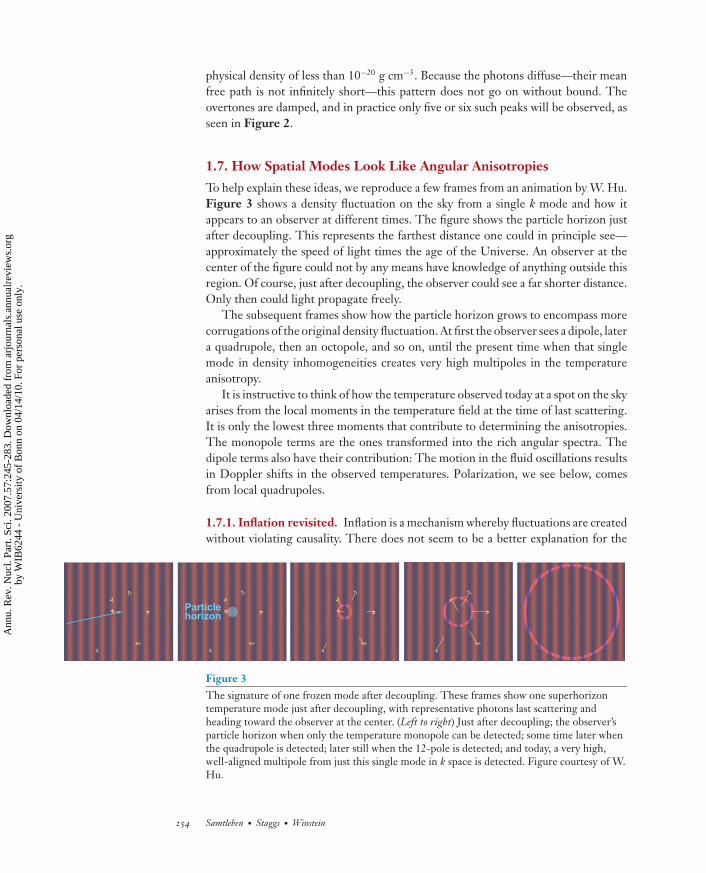
To help explain these ideas, we reproduce a few frames from an animation by W. Hu.Figure 3 shows a density fluctuation on the sky from a single k mode and how itappears to an observer at different times. The figure shows the particle horizon justafter decoupling. This represents the farthest distance one could in principle see—approximately the speed of light times the age of the Universe. An observer at thecenter of the figure could not by any means have knowledge of anything outside thisregion. Of course, just after decoupling, the observer could see a far shorter distance.Only then could light propagate freely.
The subsequent frames show how the particle horizon grows to encompass morecorrugations of the original density fluctuation. At first the observer sees a dipole, latera quadrupole, then an octopole, and so on, until the present time when that singlemode in density inhomogeneities creates very high multipoles in the temperatureanisotropy.
It is instructive to think of how the temperature observed today at a spot on the skyarises from the local moments in the temperature field at the time of last scattering.It is only the lowest three moments that contribute to determining the anisotropies.The monopole terms are the ones transformed into the rich angular spectra. Thedipole terms also have their contribution: The motion in the fluid oscillations resultsin Doppler shifts in the observed temperatures. Polarization, we see below, comesfrom local quadrupoles.
1.7.1. Inflation revisited. Inflation is a mechanism whereby fluctuations are createdwithout violating causality. There does not seem to be a better explanation for the
Particlehorizon
Figure 3The signature of one frozen mode after decoupling. These frames show one superhorizontemperature mode just after decoupling, with representative photons last scattering andheading toward the observer at the center. (Left to right) Just after decoupling; the observer’sparticle horizon when only the temperature monopole can be detected; some time later whenthe quadrupole is detected; later still when the 12-pole is detected; and today, a very high,well-aligned multipole from just this single mode in k space is detected. Figure courtesy of W.Hu.
254 Samtleben · Staggs ·Winstein
Ann
u. R
ev. N
ucl.
Part
. Sci
. 200
7.57
:245
-283
. Dow
nloa
ded
from
arj
ourn
als.
annu
alre
view
s.or
gby
WIB
6244
- U
nive
rsity
of
Bon
n on
04/
14/1
0. F
or p
erso
nal u
se o
nly.

ANRV326-NS57-09 ARI 13 September 2007 7:27
observed regularities. Nevertheless, Wolfgang Pauli’s famous statement about theneutrino comes to mind: “I have done a terrible thing: I have postulated a particlethat cannot be detected!”
Sometimes it seems that inflation is an idea that cannot be tested, or tested in-cisively. Of course Pauli’s neutrino hypothesis did test positive, and similarly thereis hope that the idea of inflation can reach the same footing. Still, we have not (yet)seen any scalar field in nature. We discuss what has been claimed as the smoking guntest of inflation—the eventual detection of gravity waves in the CMB. However, willwe ever know with certainty that the Universe grew in volume by a factor of 1063 insomething like 10−35 s?
1.8. CMB Polarization
Experiments have now shown that the CMB is polarized, as expected. Researchersnow think that the most fruitful avenue to fundamental physics from the CMB willbe in precise studies of the patterns of the polarization. This section treats the mech-anisms responsible for the generation of the polarization and how this polarization isdescribed.
1.8.1. How polarization gets generated. If there is a quadrupole anisotropy in thetemperature field around a scattering center, even if that radiation is unpolarized,the scattered radiation will be as shown in Figure 4: A linear polarization will be
xe–
z
a b
0 10
10
20
30
40
020 30 40
θX (arcmin)
θ y (
arcm
in)
0 10 20 30 40
θX (arcmin)
E mode B mode
y
Linearpolarization
Thomsonscattering
Figure 4Generation of polarization. (a) Unpolarized but anisotropic radiation incident on an electronproduces polarized radiation. Intensity is represented by line thickness. To an observer lookingalong the direction of the scattered photons (z), the incoming quadrupole pattern produceslinear polarization along the y-direction. In terms of the Stokes parameters, this is Q = (Ex
2 –Ey
2)/2, the power difference detected along the x- and y-directions. Linear polarization needsone other parameter, corresponding to the power difference between 45◦ and 135◦ from thex-axis. This parameter is easily shown to be Stokes U = ExEy. (b) E and B polarizationpatterns. The length of the lines represents the degree of polarization, while their orientationgives the direction of maximum electric field. Frames courtesy of W. Hu.
www.annualreviews.org • The CMB for Pedestrians 255
Ann
u. R
ev. N
ucl.
Part
. Sci
. 200
7.57
:245
-283
. Dow
nloa
ded
from
arj
ourn
als.
annu
alre
view
s.or
gby
WIB
6244
- U
nive
rsity
of
Bon
n on
04/
14/1
0. F
or p
erso
nal u
se o
nly.

ANRV326-NS57-09 ARI 13 September 2007 7:27
generated. The quadrupole is generated during decoupling, as shown in Figure 3. Be-cause the polarization arises from scattering but said scattering dilutes the quadrupole,the polarization anisotropy is much weaker than that in the temperature field. Indeedwith each scatter on the way to equilibrium, the polarization is reduced. Any remain-ing polarization is a direct result of the cessation of scattering. For this reason, thepolarization peaks at higher l values than does the temperature anisotropy. The localquadrupole on scales that are large in comparison to the mean free path is dilutedfrom multiple scattering.
1.8.2. The E and B polarization fields. The polarization field is both more com-plicated and richer than the temperature field. At each point in the sky, one mustspecify both the degree of polarization and the preferred direction of the electricfield. This is a tensor field that can be decomposed into two types, termed E and B,which are, respectively, scalar and pseudoscalar fields, with associated power spectra.Examples of these polarization fields are depicted schematically in Figure 4. TheE and B fields are more fundamental than the polarization field on the sky, whosedescription is coordinate-system dependent. In addition, E modes arise from the den-sity perturbations (which do not produce B modes) that we describe, whereas the Bmodes come from the tensor distortions to the space-time metric (which do have ahandedness). We mention here that the E and B fields are nonlocal. Their extractionfrom measurements of polarization over a set of pixels, often in a finite patch of sky,is a well-developed but subtle procedure (see Section 3.3).
The peaks in the EE (E-polarization correlated with itself ) spectrum should be180◦ out of phase with those for temperature: Polarization results from scatter-ing and thus is maximal when the fluid velocity is maximal. Calculating the fluidvelocity for the mode in Section 1.6, we find kEEvs tdec = π/2, 3π/2, 5π/2 . . . ,defining modes with maximal EE power. The TE (E-polarization correlated withthe temperature field) spectrum—how modes in temperature correlate with thosewith E polarization—is also of cosmological interest, with its own peak structure.Here we are looking at modes that have a maximum at decoupling in the productof their temperature and E-mode polarization (or velocity). Similarly, the appro-priate maxima (which in this case can be positive or negative) are obtained whenkTEvs tdec = π/4, 3π/4, 5π/4 . . . . Thus, between every peak in the TT power spec-trum there should be one in the EE, and between every TT and EE pair of peaksthere should be one in the TE.
1.8.3. Current understanding of polarization data. Figure 5 shows the EE re-sults in addition to the expected power spectra in the standard cosmological model.Measurements of the TE cross correlation are also shown. The pattern of peaks inboth power spectra is consistent with what was expected. What was unexpected wasthe enhancement at the lowest l values in the EE power spectrum. This is discussedin the next section.
The experiments reported in Figure 5, with 20 or fewer detectors, use a variety oftechniques and operate in different frequency ranges. This is important in dealing withastrophysical foregrounds (see Section 2) that have a different frequency dependence
256 Samtleben · Staggs ·Winstein
Ann
u. R
ev. N
ucl.
Part
. Sci
. 200
7.57
:245
-283
. Dow
nloa
ded
from
arj
ourn
als.
annu
alre
view
s.or
gby
WIB
6244
- U
nive
rsity
of
Bon
n on
04/
14/1
0. F
or p
erso
nal u
se o
nly.

ANRV326-NS57-09 ARI 13 September 2007 7:27
(l+
1)C
l/2
π (
µK2)
Multipole (l) Multipole (l)
–0.05
0
1 10 100 500 1000 1500 2000 1 10 100 500 1000 1500
0.05
0.10
0.15
–0.5
0
0.5
1.0
1.5
WMAP ('07, 40–90 GHz) 3σBOOMERANG ('06, 145 GHz) 4.8σCBI ('06, 30 GHz) 11.7σCAPMAP ('07, 90 GHz) 7.3σ preliminaryDASI ('05, 30 GHz) 6.3σ
MAXIPOL ('06, 140 GHz) 2σ
BOOMERANG ('06, 145 GHz)CBI ('06, 30 GHz)
WMAP ('07, 40–90 GHz)QUAD ('07, 100/150 GHz)
QUAD ('07, 100/150 GHz)
DASI ('05, 30 GHz)
EE TE
Figure 5Measurements of EE and TE power spectra together with the WMAP best-fit cosmologicalmodel. The names of the experiments, their years of publication, and the frequency rangescovered are indicated, as well as the number of standard deviations with which eachexperiment claims a detection. Note the change from logarithmic to linear multipole scale atl = 100 and that to display features in the very low l range, we plot (l + 1)Cl/2π .
from that of the CMB. Limits from current experiments on the B-mode power arenow at the level of 1–10 μK2, far from the expected signal levels shown in Figure 6.The peak in the power spectrum (for the gravity waves) is at l ≈ 100, the horizonscale at decoupling. The reader may wonder why the B modes fall off steeply abovethis scale and show no acoustic oscillations. The reason is simple: A tensor mode willgive, for example, a compression in the x-direction followed by a rarefaction in the y-direction, but will not produce a net overdensity that would subsequently contract. Inthe final section we discuss experiments with far greater numbers of detectors aimedspecifically at B-mode science. Note that such gravity waves have frequencies todayof order 10−16 Hz. However, if their spectrum approximates one of scale invariance,they would in principle be detectable at frequencies nearer 1 Hz, such as in the LISAexperiment. This is discussed more fully in Reference 10.
1.9. Processes after Decoupling: Secondary Anisotropies
In this section we briefly discuss three important processes after decoupling: rescat-tering of the CMB in the reionized plasma of the Universe, lensing of the CMBthrough gravitational interactions with matter, and scattering of the CMB from hotgas in Galaxy clusters. Although these can be considered foregrounds perturbing theprimordial information, each can potentially provide fundamental information.
www.annualreviews.org • The CMB for Pedestrians 257
Ann
u. R
ev. N
ucl.
Part
. Sci
. 200
7.57
:245
-283
. Dow
nloa
ded
from
arj
ourn
als.
annu
alre
view
s.or
gby
WIB
6244
- U
nive
rsity
of
Bon
n on
04/
14/1
0. F
or p
erso
nal u
se o
nly.

ANRV326-NS57-09 ARI 13 September 2007 7:27
[l(l
+1)C
l/2π
]½ (
µK)
Sensitivity ground-based ISensitivity ground-based IISensitivity spaceEEPrimordial BBLensed BB
100
10–2
10–1
100
101
101 102 103
Multipole (l)
90 10 2 1 0.1
Angular scale (°)
r = 0.3
r = 0.01
Figure 6CMB polarization power spectra and estimated sensitivity of future experiments. The solidcurves show the predictions for the E- and B-mode power spectra. The primordial B-modepower spectrum is shown for r = 0.3 and r = 0.01. The predicted B-mode signal powerspectrum due to the distortion of E modes by weak gravitational lensing is also shown.Estimated statistical sensitivities for a new space mission (pink line) and two sampleground-based experiments, as considered in Reference 9, each with 1000 detectors operatingfor one year with 100% duty cycle (dark and light blue lines), are shown. Experiment I observes4% of the sky, with a 6-arcmin resolution; experiment II observes 0.4% of the sky, with a1-arcmin resolution.
1.9.1. Reionization. The enhancement in the EE power spectrum at the very lowestl values in Figure 5 is the signature that the Universe was reionized after decoupling.This is a subject rich in astrophysics, but for our purposes it is important in thatit provides another source for scattering and hence detection of polarization. Fromthe Wilkinson Microwave Anisotropy Probe (WMAP) polarization data (11), onecan infer an optical depth of order 10%, the fraction of photons scattering in thereionized plasma somewhere in the region of z = 10. This new scattering source canbe used to detect the primordial gravity waves. The signature will show up at verylow l values, corresponding to the horizon scale at reionization. Figure 6 shows thatthe region l = 4–8 should have substantial effects from gravity waves. Most likely,the only means of detecting such a signal is from space, and even from there it willbe very difficult.
The polarization anisotropies for this very low l region are comparable to whatis expected from the surface of last scattering (l ≈ 100). There are disadvantages toeach signature. At the lowest l values, galactic foregrounds are more severe, there arefewer modes in which to make a detection, and systematic errors are likely greater.
258 Samtleben · Staggs ·Winstein
Ann
u. R
ev. N
ucl.
Part
. Sci
. 200
7.57
:245
-283
. Dow
nloa
ded
from
arj
ourn
als.
annu
alre
view
s.or
gby
WIB
6244
- U
nive
rsity
of
Bon
n on
04/
14/1
0. F
or p
erso
nal u
se o
nly.

ANRV326-NS57-09 ARI 13 September 2007 7:27
At the higher values, there is a foreground that arises from E modes turning into Bmodes through gravitational lensing (the topic of the next section). Clearly, it will beimportant to detect the two signatures with the right relative strengths at these twovery different scales.
1.9.2. Lensing of the CMB. Both the temperature and polarization fields will beslightly distorted (lensed) when passing collapsing structures in the late Universe.The bending of light means that one is not looking (on the last scattering surface)where one thinks. Although lensing will affect both the polarization and T fields,its largest effect is on the B field, where it shifts power from E to B. Gravitationaldistortions, although preserving brightness, do not preserve the E and B nature ofthe polarization patterns.
Figure 6 also shows the expected power spectrum of these lensed B modes. Be-cause this power is sourced by the E modes, it roughly follows their shape, but with�T suppressed by a factor of 20. The peak structure in the E modes is smoothed, as thestructures doing the lensing are degree scale themselves. Owing to the coherence ofthe lensing potential for these modes, there is more information than just the powerspectrum, and work is ongoing to characterize the expected cross correlation be-tween different multipole bands. This signal should be detectable in next-generationpolarization experiments.
For our purposes, the most interesting aspect of this lensing is the handle it canpotentially give on the masses of the neutrinos, as more massive neutrinos limit thecollapse of matter along the CMB trajectories. All other parameters held fixed, thereis roughly a factor-of-two change in the magnitude of the B signal for a 1-eV changein the mean neutrino mass.
1.9.3. CMB scattering since reionization. At very small angular scales—l valuesof a few thousand, way beyond where the acoustic oscillations are damped—thereare additional effects on the power spectra that result from the scattering of CMBphotons from electrons after the epoch of reionization, including scattering fromgas heated from falling deep in the potential wells of Galaxy clusters (the Sunyaev-Zel’dovich, or SZ, effect). These nonlinear effects are important as they can help inuntangling (a) when the first structures formed and (b) the role of dark energy.
1.10. What We Learn from the CMB Power Spectrum
In this section, we show how the power spectrum information is used to determineimportant aspects of the Universe. This is normally known as parameter estimation,where the parameters are those that define our cosmology. The observable powerspectrum is a function of at least 11 such basic parameters. As we discuss below, someare better constrained than others.
First, there are four parameters that characterize the primordial scalar and tensorfluctuation spectra before the acoustic oscillations, each of which is assumed to followa power law in wave number. These four are the normalization of the scalar fluctu-ations (As), the ratio of tensor to scalar fluctuations r, and the spectral indices for
www.annualreviews.org • The CMB for Pedestrians 259
Ann
u. R
ev. N
ucl.
Part
. Sci
. 200
7.57
:245
-283
. Dow
nloa
ded
from
arj
ourn
als.
annu
alre
view
s.or
gby
WIB
6244
- U
nive
rsity
of
Bon
n on
04/
14/1
0. F
or p
erso
nal u
se o
nly.

ANRV326-NS57-09 ARI 13 September 2007 7:27
both (historically denoted with ns−1 and nt). Second, there is one equation-of-stateparameter (w) that is the ratio of the pressure of the dark energy to its energy density,and one parameter that gives the optical depth (τ ) from the epoch of reionization.Finally, there are five parameters that characterize the present Universe: its rate ofexpansion (Hubble constant, with H0 = h ·100 km s−1 Mpc−1), its curvature (�k), andits composition (baryon density, matter density, and dark energy density). The latterthree are described in terms of energy densities with respect to the critical densitynormalized to the present epoch: ωb = �b h2, ωm = �mh2, and ω� = ��h2. Just 10of these are independent as �m + �� + �k = 1.
Even though the CMB data set itself consists of hundreds of measurements, theyare not sufficiently orthogonal with respect to the 10 independent parameters foreach to be determined independently; there are significant degeneracies. Hence, itis necessary to make assumptions that constrain the values of those parameters uponwhich the data have little leverage. In some cases, such prior assumptions (priors) canhave large effects on the other parameters, and there is as yet no standard means ofreporting results.
Several teams have done analyses [WMAP (11, 12), CBI (13), Boomerang (14),see also Reference 15]. Here we first discuss the leverage that the CMB power spectrahave on the cosmological parameters. Then we give a flavor for the analyses, togetherwith representative results. We consider analyses, done by the several teams, with justthe six most important parameters: ωb , ωm, As, ns, τ , and h, where the other five areheld fixed. For this discussion we are guided by Reference 12.
Completely within CMB data, there is a geometrical degeneracy between �k, acontribution to the energy density from the curvature of space, and �m. However,taking a very weak prior of h > 0.5, the WMAP team, using just their first-yeardata, determined that �k = 0.03 ± 0.03, that is, no evidence for curvature. Weassume �k = 0 unless otherwise noted. This conclusion has gotten stronger with thethree-year WMAP data together with other CMB results, and it is a prediction of theinflationary scenario. Nevertheless, we emphasize that it is an open experimental issue.
1.10.1. The geometry of the Universe. The position of the first acoustic peakreveals that the Universe is flat or nearly so. As we describe above, the generation ofacoustic peaks is governed by the (comoving) sound horizon at decoupling, rS (i.e.,the greatest distance a density wave in the plasma could traverse, scaled to today’sUniverse). The sound horizon depends on ωm, ωb , and the radiation density, but noton H0, �k, ω�, or the spectral tilt ns. The peak positions versus angular multipoleare then determined by �A = rSd−1
A , where the quantity dA, the angular diameterdistance, is the distance that properly takes into account the expansion history of theUniverse between decoupling and today so that when dA is multiplied by an observedangle, the result is the feature size at the time of decoupling. In a nonexpandingUniverse, this would simply be the physical distance. The expression depends on the(evolution of the) content of the Universe. For a flat Universe, we have
dA =∫ zdec
0
H−10 d z√
�r (1 + z)4 + �m(1 + z)3 + ��
. 5.
260 Samtleben · Staggs ·Winstein
Ann
u. R
ev. N
ucl.
Part
. Sci
. 200
7.57
:245
-283
. Dow
nloa
ded
from
arj
ourn
als.
annu
alre
view
s.or
gby
WIB
6244
- U
nive
rsity
of
Bon
n on
04/
14/1
0. F
or p
erso
nal u
se o
nly.

ANRV326-NS57-09 ARI 13 September 2007 7:27
In this expression, �r indicates the (well-known) radiation density, and the dilutionsof the different components with redshift z, between decoupling and the present,enter explicitly.
1.10.2. Fitting for spectral tilt, matter, and baryon content. It is easy to see howone in principle determines spectral tilt. If one knew all the other parameters, thenthe tilt would be found from the slope of the power spectrum after the removal ofthe other contributions. However, there is clearly a coupling to other parameters.Experiments with a very fine angular resolution will determine the power spectrumat very high l values, thereby improving the measurement of the tilt.
Here we discuss the primary dependences of the acoustic peak heights on ωm
and ωb . Increasing ωm decreases the peak heights. With greater matter density, theera of equality is pushed to earlier redshifts, allowing the dark matter more time toform deeper potential wells. When the baryons fall into these wells, their mass hasless effect on the development of the potential so that the escaping photons are lessredshifted than they would be, yielding a smaller temperature contrast. As to ωb ,increasing it decreases the second peak but enhances that of the third because theinertia in the photon-baryon fluid is increased, leading to hotter compressions andcooler rarefactions (16).
The peak-height ratios give the three parameters ns, ωm, and ωb , with a precisionjust short of that from a full analysis of the power spectrum (discussed in Section 3.4.4).Following WMAP, we define the ratio of the second to the first peak by HTT
2 , the ratioof the third to the second peak by HTT
3 , and the ratio of the first to the second peakin the polarization-temperature cross-correlation power spectrum by HTE
2 . Table 1shows how the errors in these ratios propagate into parameter errors. We see thatall the ratios depend strongly on ns, and that the ratio of the first two peaks dependsstrongly on ωb but is also influenced by ωm. For HTT
3 , the relative dependences onωb and ωm are reversed. Finally, the baryon density has little influence on the ratioof the TE peaks. However, increasing ωm deepens potential wells, increasing fluidvelocities and the heights of all polarization peaks.
Table 2 lists the results from six-parameter fits to the power spectrum from sev-eral combinations of CMB data with and without complementary data from othersectors. The table includes results from Reference 14, which included most CMBdata available at time of publication, and from even more recent analyses by WMAP(8).
Table 1 Matrix of how errors in the peak ratios(defined in text) relate to the parameter errors
ΔnsΔωbωb
Δωmωm
�HTT2 /HTT
2 0.88 −0.67 0.039�HTT
3 /HTT3 1.28 −0.39 0.46
�HTE2 /HTE
2 −0.66 0.095 0.45
www.annualreviews.org • The CMB for Pedestrians 261
Ann
u. R
ev. N
ucl.
Part
. Sci
. 200
7.57
:245
-283
. Dow
nloa
ded
from
arj
ourn
als.
annu
alre
view
s.or
gby
WIB
6244
- U
nive
rsity
of
Bon
n on
04/
14/1
0. F
or p
erso
nal u
se o
nly.
ANRV326-NS57-09 ARI 13 September 2007 7:27
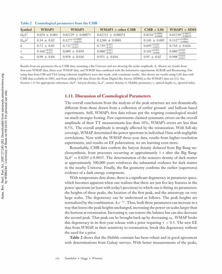
Table 2 Cosmological parameters from the CMB
Symbol WMAP1 WMAP3 WMAP3 + other CMB CMB + LSS WMAP3 + SDSS�b h2 0.024 ± 0.001 0.02229 ± 0.00073 0.02232 ± 0.00074 0.0226+0.0009
−0.0008 0.02230+0.00071−0.00070
�mh2 0.14 ± 0.02 0.1277+0.0080−0.0079 0.1260 ± 0.0081 0.143 ± 0.005 0.1327+0.0063
−0.0064
h 0.72 ± 0.05 0.732+0.031−0.032 0.739+0.033
−0.032 0.695+0.025−0.023 0.710 ± 0.026
τ 0.166+0.076−0.071 0.089 ± 0.030 0.088+0.031
−0.032 0.101+0.051−0.044 0.080+0.029
−0.030
nS 0.99 ± 0.04 0.958 ± 0.016 0.951 ± 0.016 0.95 ± 0.02 0.948+0.016−0.015
Results from six-parameter fits to CMB data, assuming a flat Universe and not showing the scalar amplitude As . Shown are results fromfirst-year WMAP data, three-year WMAP data, and WMAP data combined with the bolometric experiments ACBAR and Boomerang. Fitsusing data from CBI and VSA (using coherent amplifiers) were also made, with consistent results. Also shown are results using LSS data withCMB data available in 2003, and from adding LSS data [from the Sloan Digital Sky Survey (SDSS)] to the WMAP3 data set (11). SeeSection 1.11 for appropriate references. �b h2, baryon density; �mh2, matter density; h, Hubble parameter; τ , optical depth; nS, spectral index.
1.11. Discussion of Cosmological Parameters
The overall conclusions from the analysis of the peak structure are not dramaticallydifferent from those drawn from a collection of earlier ground- and balloon-basedexperiments. Still, WMAP’s first data release put the reigning cosmological modelon much stronger footing. Few experiments claimed systematic errors on the overallamplitude of their TT measurements less than 10%; WMAP’s errors are less than0.5%. The overall amplitude is strongly affected by the reionization. With full-skycoverage, WMAP determined the power spectrum in individual l bins with negligiblecorrelations. Now with the WMAP three-year data, results from higher-resolutionexperiments, and results on EE polarization, we are learning even more.
Remarkably, CMB data confirm the baryon density deduced from Big Bang nu-cleosynthesis, from processes occurring at approximately 1 s after the Big Bang:�b h2 = 0.0205 ± 0.0035. The determination of the nonzero density of dark matterat approximately 300,000 years reinforces the substantial evidence for dark matterin the nearby Universe. Finally, the flat geometry confirms the earlier (supernova)evidence of a dark energy component.
With temperature data alone, there is a significant degeneracy in parameter space,which becomes apparent when one realizes that there are just five key features in thepower spectrum (at least with today’s precision) to which one is fitting six parameters:the heights of three peaks, the location of the first peak, and the anisotropy on verylarge scales. The degeneracy can be understood as follows. The peak heights arenormalized by the combination As e−2τ . Thus, both these parameters can increase in away that leaves the peak heights unchanged, increasing the power on scales larger thanthe horizon at reionization. Increasing ns can restore the balance but can also decreasethe second peak. That peak can be brought back up by decreasing ωb . WMAP brokethis degeneracy in its first-year release with a prior requiring τ < 0.3. The new EEdata from WMAP, in their sensitivity to reionization, break this degeneracy withoutthe need for a prior.
Table 2 shows that the Hubble constant has been robust and in good agreementwith determinations from Galaxy surveys. With better measurements of the peaks,
262 Samtleben · Staggs ·Winstein
Ann
u. R
ev. N
ucl.
Part
. Sci
. 200
7.57
:245
-283
. Dow
nloa
ded
from
arj
ourn
als.
annu
alre
view
s.or
gby
WIB
6244
- U
nive
rsity
of
Bon
n on
04/
14/1
0. F
or p
erso
nal u
se o
nly.

ANRV326-NS57-09 ARI 13 September 2007 7:27
the baryon and matter densities have moved systematically, but within error. Theoptical depth has decreased significantly and is now based upon the EE, rather thanTE, power in the lowest l range. This change is coupled to a large change in the scalaramplitude. Finally, evidence for a spectral tilt (ns �= 1) is becoming more significant.As this is predicted by the simplest of inflationary scenarios, it is important anddefinitely worth watching.
The first-year WMAP data confirmed the COBE observation of unexpectedly lowpower in the lowest multipoles. The WMAP team reported this effect to be moresignificant than a statistical fluctuation, and lively literature on the subject followed.It is it clear that the quadrupole has little power and appears to be aligned with theoctopole. However, the situation is unclear in that the quadrupole lines up reasonablywell with the Galaxy itself, and there is concern that the cut on the WMAP data toremove the Galaxy then reduced the inherent quadrupole power. The anomaly hasbeen reduced with the three-year data release, with improvements to the analysis,particularly in the lowest multipoles.
Table 2 also gives results from fitting CMB data with data from other cosmologicalprobes, in particular large-scale structure (LSS) data in the form of three-dimensionalGalaxy power spectra (the third dimension is redshift). Such spectra extend the leverarm in k space, allowing a more incisive determination of any possible spectral tilt, ns.However, there are potential biases with the Galaxy data. In particular, the galaxiesmay not be faithful tracers of the dark matter density. Already before the three-yearWMAP data release, including LSS data with CMB data favored an optical depthcloser to its current value and provided evidence of spectral tilt. With three-yearWMAP data and the Sloan Digital Sky Survey Galaxy survey data, the significanceof a nonzero tilt is near the 3σ level. This is a vigorously debated topic. There areother LSS surveys that give similar and nearly consistent results, yet the systematicunderstanding is not at the level where combining all such surveys makes sense.
1.11.1. Beyond the six basic parameters. With the LSS data, one can obtain infor-mation on other parameters that were held fixed. In particular, relaxing the constrainton �k, one finds consistency with a flat Universe to the level of approximately 0.04(with CMB data alone) and 0.02 (using LSS data) (see Reference 14). Using WMAPand other surveys, constraints as low as 0.015 are obtained with some sets, givingslight indications for a closed Universe (�k < 0).
There is sensitivity to the fraction of the dark matter that resides in neutrinos: fv.The neutrino number density (in the standard cosmological model) is well known;a mean neutrino mass of 0.05 eV corresponds to �ν of approximately 0.001. Thecurrent limits are Mν < 1 eV from the CMB alone and Mν < 0.4 eV when includingGalaxy power spectra (14).
One can also extract information about the dark energy equation-of-state param-eter w. If dark energy is Einstein’s cosmological constant, then w ≡ −1. Because waffects the expansion history of the Universe at late times, the associated effects onpower spectra then give a measure of w. Using all available CMB data, Reference 14finds w = −0.86+0.35
−0.36. However, by including both the Galaxy power spectra andSN1A data, the stronger constraint w = −0.94+0.093
−0.097 is derived. WMAP, using its
www.annualreviews.org • The CMB for Pedestrians 263
Ann
u. R
ev. N
ucl.
Part
. Sci
. 200
7.57
:245
-283
. Dow
nloa
ded
from
arj
ourn
als.
annu
alre
view
s.or
gby
WIB
6244
- U
nive
rsity
of
Bon
n on
04/
14/1
0. F
or p
erso
nal u
se o
nly.

ANRV326-NS57-09 ARI 13 September 2007 7:27
own data and another collection of LSS data together with supernova data, finds w =−1.08 ± 0.12, where in this fit they also let �k float.
Finally, we want to mention a new effect, even if outside the domain of the CMB—baryon oscillations. In principle, one should be able to see the same kind of acousticoscillations in baryons (galaxies) seen so prominently in the radiation field. If so, thiswill provide another powerful measure of the effects of dark energy at late times,specifically the time when its fraction is growing and its effects in curtailing structureformation are the largest. This effect has recently been seen (17) at the level of 3.4σ ,and new experiments to study this far more precisely are being proposed. This is anexcellent example of how rapidly the field of observational cosmology is developing.In the wonderful textbook Modern Cosmology by Scott Dodelson (2, p. 209), Dodelsonstates that this phenomenon would only be “barely (if at all) detectable.”
Before turning to a discussion of the problem of astrophysical foregrounds, wemention that currently the utility of ever more precise cosmological-parameter deter-mination is, like in particle physics, not that we can compare such values with theorybut rather that we can either uncover inconsistencies in our modeling of the physicsof the Universe or gain ever more confidence in such modeling.
2. FOREGROUNDS
Until now, we have introduced the features of the CMB, enticing the reader with itspromises of fascinating insights to the very early Universe. Now we turn our attentiontoward the challenge of actually studying the CMB, as its retrieval is not at all an easyendeavor. Instrumental noise and imperfections could compromise measurements ofthe tiny signals (see Section 3). Even with an ideal receiver, various astrophysical oratmospheric foregrounds could contaminate or even suppress the CMB signal. Inthis section we first give an overview of the relevant foregrounds, then describe theoptions for foreground removal and estimate their impact.
2.1. Overview
One may be tempted to observe the CMB at its maximum, approximately 150–200 GHz. However, atmospheric, galactic, or extragalactic foregrounds, which havetheir own dependences on frequency and angular scale, may dominate the total signal,so the maximum may not be the best choice.
The main astrophysical foregrounds come from our own Galaxy, from threedistinct mechanisms: synchrotron radiation; radiation from electron-ion scattering,usually referred to as free-free emission; and dust emission. Figure 7 displays full-sky intensity maps for the main foreground components as derived from WMAPdata at microwave frequencies where the bright Galaxy is clearly dominating thepictures. Each component is shown for the WMAP frequency channel where it isdominant.
Figure 8 compares the expected CMB signal as a function of frequency to therms of WMAP foreground maps on an angular scale of 1◦. The ordinate axis recordsantenna temperature (see Section 3.2.1). An optimal observing frequency range with
264 Samtleben · Staggs ·Winstein
Ann
u. R
ev. N
ucl.
Part
. Sci
. 200
7.57
:245
-283
. Dow
nloa
ded
from
arj
ourn
als.
annu
alre
view
s.or
gby
WIB
6244
- U
nive
rsity
of
Bon
n on
04/
14/1
0. F
or p
erso
nal u
se o
nly.

ANRV326-NS57-09 ARI 13 September 2007 7:27
Synchrotron(K-band, 23 GHz)
Free-free(K-band, 23 GHz)
Dust(W-band, 94 GHz)
Figure 7Unpolarized foreground maps in Galactic coordinates, derived from WMAP. Each map isshown at the WMAP frequency band in which that foreground is dominant. The color scalefor the temperature is linear, with maxima set at approximately 5 mK for K-band and 2.5 mKfor W-band. Images courtesy of the WMAP science team.
the highest ratio of CMB to foreground signal is in the region around 70 GHz (oftentermed the cosmological window).
Much less is known about the polarization of foregrounds. Information is extrapo-lated mostly from very low or very high frequencies or from surveys of small patches.Figure 8b shows an analog figure for the polarization fluctuations as estimated fromWMAP three-year data on an angular scale of approximately 2◦ (l = 90), where thesignal from gravitational waves is maximal. The dust estimate has some limitationsbecause the WMAP frequency channels do not extend to the high frequencies wherethe dust is expected to dominate the foregrounds.
K Ka Q V W
CMB anisotropy85% sky (Kp2)
77% sky (Kp0)
Free-free Dust
Synchrotron
a b
[l(l
+1)C
l/2π
]½ (
µK
)
An
ten
na
tem
per
atu
re(µ
K, r
ms)
20 40 60 80 100 20020200
10–2
10–3
10–1
100
101
100
101
102
Frequency (GHz)Frequency (GHz)
r = 0.1
r = 0.01
r = 0.001
WMAP polarized foreground estimatesat l = 90
BB dustEE dustEE synchrotron BB synchrotronEE sum BB sum
Figure 8Frequency dependence of foregrounds recorded in antenna temperature. (a) The rms onangular scales of 1◦ for the unpolarized CMB compared with that from foregrounds extractedfrom the WMAP data (18). The WMAP frequency bands (K, Ka, Q, V, W) are overlaid aslight bands. These plots are for nearly full sky; the total foregrounds are shown as dashed linesfor two different sky cuts. Figure courtesy of the WMAP science team. (b) A similar plot of theexpected polarization level of foregrounds at l = 90 in comparison with that from primordialB modes (which peak around l = 90) for different values of r following formula 25 inReference 19. Again, these estimates are for observations covering most of the sky.
www.annualreviews.org • The CMB for Pedestrians 265
Ann
u. R
ev. N
ucl.
Part
. Sci
. 200
7.57
:245
-283
. Dow
nloa
ded
from
arj
ourn
als.
annu
alre
view
s.or
gby
WIB
6244
- U
nive
rsity
of
Bon
n on
04/
14/1
0. F
or p
erso
nal u
se o
nly.
ANRV326-NS57-09 ARI 13 September 2007 7:27
The expected B-mode signal is smaller than the estimated foreground signal evenfor r = 0.1. However, almost the full sky was used for the estimate, whereas re-cent studies (20, 21) using lower-frequency data and WMAP data indicate that thepolarization of synchrotron radiation on selected clean patches can be significantlysmaller. Thus, the optimal frequency window will shift depending on which region isobserved. After discussing possible foreground effects from Earth’s atmosphere, webriefly review what is known about the dominant sources of galactic and extragalacticforegrounds.
2.1.1. Atmospheric effects. The atmosphere absorbs short-wavelength radiation,but fortunately has transmission windows in the range of visible light and microwaveradiation. Absorption lines from oxygen (around 60 and 120 GHz) and water vapor (20and 180 GHz) limit the access to the microwave sky, and, in particular, clouds and highwater vapor can compromise ground-based observations. Thermal emission from theatmosphere can add significantly to the observed signal for ground-based experiments(depending on the observing site and the frequency, from 1–40 K) and, together withthe instrumental noise and/or thermal emission from warm optical components, canmake for the major part of the detected power (see also Section 3.2.1). The observingstrategy needs to be designed in a way that allows a proper removal of the varyingatmospheric contribution without a big impact on the signal extraction (see alsoSections 3.3 and 3.4.1).
Although thermal emission from the atmosphere is unpolarized, the Zeeman split-ting of oxygen lines in Earth’s magnetic field leads to polarized emission, which isdominantly circularly polarized. Although the CMB is not expected to be circularlypolarized, Hanany & Rosenkranz (22) showed that for large angular scales, l ≈ 1, a0.01% circular-to-linear polarization conversion in the instrument could produce asignal more than a factor of two higher than the expected gravitational wave B-modesignal if r were small, that is, if r = 0.01.
In addition, backscattering of thermal radiation from Earth’s surface from icecrystal clouds in the upper troposphere may give signals on the order of micro-Kelvinsize (23), again larger than the expected B-mode signal. Although the polarized signalfrom oxygen splitting would be fixed in Earth’s reference frame, and thus could beseparated from the CMB, the signal from such ice clouds would reflect the varyinginhomogeneous cloud distribution and thus be hard to remove.
2.1.2. Galactic synchrotron radiation. Synchrotron radiation is something familiarto particle physicists, mostly from storage rings where some of the energy meant toboost the particle’s energy will be radiated away. The same effect takes place in galacticaccelerators, with cosmic-ray electrons passing through the galactic magnetic field.In contrast to the particle physics case, where electrons of energies of a few GeV passmagnetic fields of up to a few 1000 G, we are dealing here with electrons in a galacticfield of only a few micro-Gauss.
This component of the foreground radiation is dominant at frequencies be-low 70 GHz, and its intensity characteristics have been studied at frequencies
266 Samtleben · Staggs ·Winstein
Ann
u. R
ev. N
ucl.
Part
. Sci
. 200
7.57
:245
-283
. Dow
nloa
ded
from
arj
ourn
als.
annu
alre
view
s.or
gby
WIB
6244
- U
nive
rsity
of
Bon
n on
04/
14/1
0. F
or p
erso
nal u
se o
nly.

ANRV326-NS57-09 ARI 13 September 2007 7:27
up to 20 GHz, The frequency and angular dependence both follow power lawsT ∝ ν−β , with a position- and frequency-dependent exponent that varies between2 and 3.
Theoretically, a high degree of sychrotron polarization (>75%) is expected, butlow-frequency data imply much lower values. However, at low frequencies, Faradayrotation—where light traversing a magnetized medium has its left and right circularpolarized components travel at different speeds—reduces the polarization.
2.1.3. Galactic dust. Interstellar dust emits mainly in the far infrared and thus be-comes relevant for high frequencies (v > 100 GHz). The grain size and dust temper-ature determine the properties of the radiation, where the intensity follows a powerlaw T ∝ T0ν
β , with the spectral index β ≈ 2 and with both T0 and β varying overthe sky. Using far-infrared data from COBE, Finkbeiner et al. (24) (FDS) provided amodel for the dust emission consisting of two components of different temperatureand emissivity (T = 9.4/16 K, β = 1.67/2.7).
There are also indications for another component in the dust emission, as seenthrough cross correlation of the CMB and far-infrared data. Its spectral index is con-sistent with free-free emission, but it is spatially correlated with dust. This anomalousdust contribution could derive from spinning dust grains. However, current data donot provide a conclusive picture, and additional data in the 5–15-GHz range areneeded to better understand this component (25).
In 2003, the balloon-borne experiment ARCHEOPS reported 5% to 20% polar-ization of the submillimeter diffuse galactic dust emission, providing the first largecoverage maps of polarized galactic submillimeter emission at 13′ resolution (26).More recently, they also published submillimeter polarization limits at large angularscales, which when extrapolated to 100 GHz are still much larger than the expectedgravitational wave signal for r = 0.3 (27).
2.1.4. Free-free emission. Electron-ion scattering leads to radiation that is, in thiscontext, termed free-free emission, whereas in the high-energy lab, it is better knownas bremsstrahlung. This component does not dominate the foregrounds at any radiofrequency. Sky maps of free-free emission can be approximated using measurementsof the Hα emission (from the hydrogen transition from n = 3 to n = 2), which tracesthe ionized medium. The thermal free-free emission follows a power law T ∝ ν−β ,where β ≈ 2. This foreground is not polarized.
2.1.5. Point sources. Known extragalactic point sources are a well-localized con-taminant and easily removable. However, the contribution from unresolved pointsources can severely affect measurements: for example, the recent discussion of theirimpact on the determination of ns from WMAP data (28). Point sources impact CMBmeasurements mostly at high angular scales and low frequencies. For low frequen-cies, their contribution may still be larger than the signal expected from gravitationalwaves.
www.annualreviews.org • The CMB for Pedestrians 267
Ann
u. R
ev. N
ucl.
Part
. Sci
. 200
7.57
:245
-283
. Dow
nloa
ded
from
arj
ourn
als.
annu
alre
view
s.or
gby
WIB
6244
- U
nive
rsity
of
Bon
n on
04/
14/1
0. F
or p
erso
nal u
se o
nly.
ANRV326-NS57-09 ARI 13 September 2007 7:27
2.2. Foreground Removal
Understanding and removing foregrounds are most critical for the tiny polarizationsignals. The different frequency dependences of the CMB and galactic foregroundsprovide a good handle for foreground removal using multifrequency measurements.
For the polarization analysis, methods where little or no prior information isrequired are the most useful for now. A promising strategy is the Independent Com-ponent Analysis, which has already been applied to several CMB temperature datasets (including COBE, BEAST, and WMAP) and for which formalism has also beendeveloped to cope with polarization data. The foreground and CMB signals are as-sumed to be statistically independent, with at least one foreground component beingnon-Gaussian. Then the maximization of a specific measure of entropy is used to dis-entangle the independent components. Stivoli et al. (29) demonstrated a successfulcleaning of foregrounds using simulated data. Verde et al. (30) estimated the impactof foregrounds independent of removal strategy, considering different degrees of ef-fectiveness in cleaning. A 1% level of residual foregrounds, in their power spectrum,was found to be necessary to obtain a 3σ detection of r = 0.01 from the ground.
Because all current studies rely on untested assumptions about foregrounds, theyneed to be justified with more data. Moreover, none of the studies to date takesinto account the impact of foregrounds in the presence of lensing and instrumentalsystematics. Work is needed on both the experimental and theoretical side to obtaina more realistic picture of the foregrounds and their impact.
3. METHODS OF DETECTION
We have argued that in the patterns of the CMB lies greatness; here we outline theessential ingredients for measuring CMB anisotropies. The fundamental elementsfor detecting microwave emission from the celestial sphere are optics and receivers.The optics comprises telescopes and additional optical elements that couple lightinto the receivers. The receivers transduce the intensity of the incoming microwaveradiation into voltages that can be digitized and stored. Two other CMB experimentrequirements are fidelity control (calibration and rejection of spurious signals) andoptimized strategies for scanning the telescope beams across the rotating sky. Below,after a general introduction to the problem, we elaborate on these topics and culminatewith an overview of data analysis techniques.
3.1. The CMB Experiment Basics
All CMB experiments share certain characteristics. Some main optical element deter-mines the resolution of the experiment. This main optical element may be a reflectingtelescope with a single parabolic mirror, or one with two or more mirrors; it may bea refracting telescope using dielectric lenses; it may be an array of mirrors config-ured as an interferometer; it may be just a horn antenna.2 In most cases, additional
2A horn antenna is waveguide flared to the appropriate aperture for the desired resolution; these were usedin the COBE satellite instrument that made the first detection of CMB anisotropy.
268 Samtleben · Staggs ·Winstein
Ann
u. R
ev. N
ucl.
Part
. Sci
. 200
7.57
:245
-283
. Dow
nloa
ded
from
arj
ourn
als.
annu
alre
view
s.or
gby
WIB
6244
- U
nive
rsity
of
Bon
n on
04/
14/1
0. F
or p
erso
nal u
se o
nly.

ANRV326-NS57-09 ARI 13 September 2007 7:27
optical elements are required to bring the light to the receiver. Examples includeDewar windows, lenses, filters, polarization modulators, and feedhorns (which arehorn antennas used to collect light from telescopes). Typically these coupling opticsare small enough that they can be maintained at cryogenic temperatures to reducetheir thermal emission and lossiness.
The low-noise receivers are nearly always cryogenic and divide into two types,described below. Spatial modulation of the CMB signal on timescales of less than oneminute is critical to avoid slow drifts in the responsivity of the receivers, and mayproceed by movement of the entire optical system, or by moving some of its compo-nents while others remain fixed. Large ground screens surround most experimentsto shield the receivers from the 300-K radiation from Earth. Typically, the thermalenvironment of the experiment must be well regulated for stability of the receiverresponsivity and to avoid confusion of diurnal effects from the environment withthe daily rotation of the celestial signal. Earth-bound experiments suffer the excessnoise from the atmosphere, as well as its attenuation of the signal, and must contendwith 2π of the 300-K radiation. Balloon-borne experiments suffer less atmosphere,but must be shielded from the balloon’s thermal radiation and typically have limitedlifetimes (1–20 days). Long flights usually require constant shielding from the Sunduring the long austral summer day. Space missions have multiple advantages: noatmosphere, Earth filling a much less solid angle, a very stable thermal environment,and a longer lifetime than current balloon missions.
3.2. The Detection Techniques
Although to fully describe the CMB anisotropies requires their spatial power spec-tra (which happily are not white), a useful order-of-magnitude number is that therms of the CMB sky when convolved to 10◦ scales is approximately 30 μK, and ap-proximately 70 μK for 0.7◦ scales (the first acoustic peak). This rms of the CMBtemperature is some 20 ppm of the 2.7-K background, the polarization E modesare 20 times lower, and the primordial B-mode rms is predicted to be 50 ppb orless.
A microwave receiver measures one or more of the Stokes parameters of the ra-diation incident on it. Two classes of low-noise receivers may be identified: coherentreceivers, in which phase-preserving amplification of the incident field precedes de-tection of its intensity, and incoherent receivers, in which direct measurement of theintensity of the incident field is performed.
In coherent receivers, the incident field is piped around transmission lines as atime-varying voltage. That voltage is amplified in transistor amplifiers, and then thesignal is eventually detected when it passes through a nonlinear element (such as adiode) with an output proportional to the square of the incident field strength. Thecritical element in the coherent receiver is not the detector but typically the transistoramplifier, which must be a low-noise amplifier. In cases where transistor amplifiersare not available at high enough frequencies, the first and most critical element in thereceiver is a low-noise mixer, which converts the frequency of the radiation to lowerfrequencies, where low-noise amplifiers are available.
www.annualreviews.org • The CMB for Pedestrians 269
Ann
u. R
ev. N
ucl.
Part
. Sci
. 200
7.57
:245
-283
. Dow
nloa
ded
from
arj
ourn
als.
annu
alre
view
s.or
gby
WIB
6244
- U
nive
rsity
of
Bon
n on
04/
14/1
0. F
or p
erso
nal u
se o
nly.

ANRV326-NS57-09 ARI 13 September 2007 7:27
For the CMB, the most widely used incoherent detector to date is the bolometer.A bolometer records the intensity of incident radiation by measuring the temperaturerise of an isolated absorber of the radiation. A promising effort is underway to developreceivers in which the bolometers are coupled to transmission lines, where they canserve as the very low-noise detectors in what otherwise looks like a coherent receiver.
3.2.1. Calibration, Kelvins, and system temperature. A microwave receiver out-puts a voltage proportional to the intensity I of the incident radiation over someeffective bandwidth �ν centered on frequency v0. The output is calibrated in temper-ature units through observation of blackbody sources. The polarization anisotropiesof the CMB are also described in temperature units. This follows because the Stokesparameters Q and U have the same units as the intensity I. There is a factor of twoto keep track of: The usual definition of I sums the intensities from two orthogonalpolarization modes. Note that the antenna temperature TA is defined by the approx-imation I ∝ TA. Only in the Rayleigh-Jeans regime of a blackbody does TA ≈ T, butit is a convenient measure for comparing the effects of various foregrounds and othercontaminants.
Microwave receivers are sensitive to the total intensity of the incident radiationover the bandpass. The incident electric field can be considered as a sum of incoherent(i.e., uncorrelated) sources, each with intensity that can be associated to a temperaturein the Rayleigh-Jeans limit. Thus, we can define the system temperature to describethe input power to the receiver:
Tsys = TCMB + Tfg + Tatm + Tgnd + Topt + Tn, 6.
where we have included terms for the CMB, foregrounds, atmosphere, 300-K emis-sion from the ground, emission from the warm optics, and receiver, respectively. Wedo not note explicitly that the extra-atmospheric signals are attenuated slightly asthey pass through the atmosphere. At good sites such as the Atacama Desert in Chileor the South Pole, this effect is small for v = 110 GHz. We also neglect absorptionin the optics, although in bolometer systems, this effect can be large. Note that whendescribing bolometer receivers, it is more common to leave the sum in units of power,as we see below.
3.2.2. Sensitivity and noise. Imagine a CMB experiment that scans across a smallenough region of sky that the sky curvature may be neglected, recording the temper-ature of each of N beam-sized patches of sky a single time into a vector d. The erroron each measurement is σe . Let us first take the (unattainable) case where σe � 1 nK.In that case, σ 2
d measures the variance of the CMB itself. If the CMB power spec-trum were white with average level �T 2, for example, the variance could be crudelyestimated as
σ 2d ≈ �T 2 δ�
�c, 7.
where �c is some average � in the region δ� between (xb )−1 and (Nxb )−1, with xb thediameter of the beam-sized patch in radians. Typical numbers might give δ�/�c ≈ 1,and �T = 60 μK ≈ σd . Thus, for σe so small, one could estimate the Fourier modes
270 Samtleben · Staggs ·Winstein
Ann
u. R
ev. N
ucl.
Part
. Sci
. 200
7.57
:245
-283
. Dow
nloa
ded
from
arj
ourn
als.
annu
alre
view
s.or
gby
WIB
6244
- U
nive
rsity
of
Bon
n on
04/
14/1
0. F
or p
erso
nal u
se o
nly.

ANRV326-NS57-09 ARI 13 September 2007 7:27
(or the C� themselves) directly and trace out details of the spectrum over the rangeδ�.
To consider a more realistic case, we note that CMB receivers are characterizedaccording to their sensitivity S in units of K
√s . The variance σ 2
T of a series of mea-surements, each resulting from an integration time τ , is then found by σ 2
T = S/τ . Atypical value for the sensitivity of a single receiver is 500 μK/
√s , so that after 10 min
on each patch, one might attain σe ≈ 20 μK and then detect the CMB signal excessvariance in the data. Typical variances in the CMB E polarization are (4 μK)2, so theseexperiments must integrate for hundreds of hours and/or use hundreds of receivers.The tougher sensitivity requirements for B modes are described in Section 4.
In cases where the mean photon mode occupancy n0 for the input radiation is large,n0 = (ex – 1)−1 1 with x = hν/(kTsys), we can describe classically the sensitivity ofan ideal direct receiver of bandwidth �ν with the Dicke equation: S = Tsys/
√�ν. We
account for more complex receivers below. Most coherent receivers operate in thelimit n0 1. In cases where n0 � 1 (low Tsys and high frequency v), the limitationto sensitivity in ideal bolometric receivers comes from photon shot noise (countingstatistics), and the sensitivity depends on
√Tsys in cases where the bolometer thermal
noise is negligible. We return to the noise in bolometers below.The sensitivity of the receiver captures its best features succinctly. It is also in-
structive to look at the spectra of postdetection signal noise from the receivers. Thescanning of the telescope translates the CMB anisotropy signal to variations in timethat lie atop the intrinsic postdetection noise. A typical noise power spectrum is shownin Figure 9. This spectrum shows a white-noise level at frequencies f > 0.01 Hz; thesensitivity is measured from the white noise. The spectrum also shows characteristiclow-frequency noise approximately proportional to 1/f, which can be parametrizedby the frequency fc where the 1/f and white-noise powers are equal. Such 1/f noiseis ubiquitous; the atmosphere itself has a 1/f spectrum. In principal, this noise isquite serious, as it contributes more and more to the variance with longer integrationtimes. In practice, experiments are designed to modulate the signal at frequenciesf > fc. Usually the receiver includes a low-pass filter that limits the bandwidth ofthe postdetection data stream to fNy. Then these data are Nyquist sampled and dig-itized at a rate of 2fNy to avoid aliasing high-frequency noise. Roughly speaking, thepostdetection bandwidth of interest is usually between 0.01–0.1 Hz and 50–200 Hz.
3.2.3. Coherent receivers. A key advantage of coherent receivers is that they canbe configured so that their output is the correlation of two input signals. We devotethe bulk of our discussion here to this topic.
Coherent-receiver noise spectra. The noise properties of amplifiers include bothintrinsic output voltage fluctuations, present in principle even in the absence of inputsignal3 and characterized by Tn, and fluctuations in the gain coefficient (the factor by
3We remind the reader that for the frequencies of interest, “absence of input signal” is a difficult requirementbecause a resistive termination emits thermal radiation, whereas a shorted input reflects back any thermalradiation emitted from the amplifier input.
www.annualreviews.org • The CMB for Pedestrians 271
Ann
u. R
ev. N
ucl.
Part
. Sci
. 200
7.57
:245
-283
. Dow
nloa
ded
from
arj
ourn
als.
annu
alre
view
s.or
gby
WIB
6244
- U
nive
rsity
of
Bon
n on
04/
14/1
0. F
or p
erso
nal u
se o
nly.

ANRV326-NS57-09 ARI 13 September 2007 7:27
Bias lines
Celestialradiation
Thermometer
Bolometer
Cold reservoir
Microwave absorber:heat capacity C (pJ/K)
Frequency (Hz)
Po
wer
sp
ectr
um
(K
2 H
z–1)
10–3
10–4
10–5
10–6
100
10–1
10–2
10–410–5 10–3 10–2 10–1 100 101 102
Thermally conducting strap:conductance G (pW/K)
Tbath
Figure 9(Left) Raw postdetection noise power spectrum from a correlation polarimeter during scans ofthe sky, illustrating three interesting features: its white-noise level at frequency f > 0.01 Hz, apeak corresponding to the scan period of 21 s, and the characteristic low-frequency noise withslope 1/f. Figure courtesy of C. Bischoff and the CAPMAP team (31). (Right) Sketch of abolometer, indicating that celestial radiation is absorbed in a material with heat capacity Ccoupled to a cold reservoir at temperature Tbath by a strap with low thermal conductance G. Athermometer measures the power delivered to the absorber by recording its temperatureincrease.
which the input voltage is amplified). An extension of the Dicke equation reads
δT = aTsys
√1
�ντ+
(δgg
)2
, 8.
where the coefficient a depends on the exact configuration of the receiver; a = 1 for adirect receiver in which the input is amplified and then detected. For the correlationpolarimeters described below, a = √
2.
Signal correlation. Two signals are correlated if the time average of their prod-uct is nonzero. In 1952, Ryle (32) introduced the concept of phase switching: pe-riodically introducing a half-wavelength phase lag into one of the two signal lines,which changes the sign of the correlation product. Then, one can sum the two inputsand square them in a detector diode. The correlation product is now modulated atthe phase-switching rate and may be recovered. The correlation can also be mea-sured in analog correlators (multipliers) or by digitization of the inputs, followed bymultiplication.
272 Samtleben · Staggs ·Winstein
Ann
u. R
ev. N
ucl.
Part
. Sci
. 200
7.57
:245
-283
. Dow
nloa
ded
from
arj
ourn
als.
annu
alre
view
s.or
gby
WIB
6244
- U
nive
rsity
of
Bon
n on
04/
14/1
0. F
or p
erso
nal u
se o
nly.

ANRV326-NS57-09 ARI 13 September 2007 7:27
Correlation receivers. Correlation receivers have been used in several ways to mea-sure CMB signals. We describe two methods below. The advantages of correlation in-clude reduced sensitivity to 1/f variations in amplifiers (because phase switching withdiode switches can be effected at kilo-Hertz rates), reduced sensitivity to gain fluc-tuations (because those fluctuations multiply only the small correlated signal ratherthan the large, common-mode intensity signal), and the ability to access all four ofthe Stokes parameters that describe the full polarization state of the radiation usingonly two inputs.
Interferometers. Perhaps the best-known example of signal correlation in astron-omy lies in the interferometer, which uses the correlation of signals from two spa-tially separated telescopes to measure Fourier modes of the celestial radiation in alimited field of view. The interferometer’s receiver detects a slice of the interferencepattern that arises when the two input signals originate with phase coherence, muchas the screen in a Young’s diffraction experiment does. The angular resolution is de-termined by the spacing between the telescopes, whereas the size of the individualtelescopes limits the field of view. The resolution of an interferometer may be de-scribed in terms of its synthesized beamwidth, σb . Because the CMB is an extendedsource, nearly all the Fourier modes in the field of view are needed to fully charac-terize it. All the Fourier modes can be measured only if the individual telescopes areclose packed so that they fill all the space required for an equivalent single dish ofresolution σb .
To recover all four Stokes parameters, the telescope optics usually includes cir-cular polarizers so that a given receiver amplifies either the left (L) or right (R) cir-cular polarization state. Both DASI and CBI used quarter-wave plates in the opticsto periodically reverse the polarization state, L ↔ R, so that all possible combi-nations of correlations (LR, LL, RR, and RL) could be measured from each pair oftelescopes.
Correlation polarimeters. In a correlation polarimeter, the incident signal entersthrough an azimuthally symmetric feedhorn and is separated into two polarizationstates (either two orthogonal linear polarization states or the L and R circular polar-ization states) before amplification in high-electron-mobility-transistor amplifiers.After amplification, the two polarization states are correlated so that the output isproportional to a linear Stokes parameter: Vout ∝ ±Ex Ey ∝ ±U, with the modula-tion provided by the phase switch. Figure 9 shows the stability of a phase-switchedcorrelation polarimeter, switched at 4 kHz. The high-electron-mobility-transistoramplifiers in this polarimeter have 1/f knees at 1 kHz and cannot be used without thisrapid modulation. The sensitivity of this polarimeter is found from the Dicke equa-tion with a = √
2. If L and R states are used, then the second linear Stokes parametercan also be obtained by phase shifting R by an extra π/2 and then correlating it withL. The correlation can come about either through direct multiplication of the twopolarization states or through the Ryle technique. The QUIET project uses the lattermethod, in which L and R are sent into a compact module that mounts onto a circuitboard. The correlation LR is constructed by differencing the squares of the sum and
www.annualreviews.org • The CMB for Pedestrians 273
Ann
u. R
ev. N
ucl.
Part
. Sci
. 200
7.57
:245
-283
. Dow
nloa
ded
from
arj
ourn
als.
annu
alre
view
s.or
gby
WIB
6244
- U
nive
rsity
of
Bon
n on
04/
14/1
0. F
or p
erso
nal u
se o
nly.
ANRV326-NS57-09 ARI 13 September 2007 7:27
difference terms L + R and L − R; U is found by similar means. Phase switches at4 kHz modulate the outputs, which are read out on module pins; other module pinsare used to bias the amplifiers.
3.2.4. Incoherent detectors. A number of clever ideas beyond the scope of thisreview are being pursued for tailoring bolometers to search for CMB polarization.One recent great success was the advent of the polarization-sensitive bolometer.Another avenue is using wafer-level silicon fabrication techniques to produce arraysof hundreds of detectors at once, sometimes coupling the detectors directly to planarantennas or antenna arrays (antenna-coupled bolometers). Below we focus on therudiments of the transition edge sensor (TES) bolometer.
Figure 9 depicts the critical elements of a bolometer. Celestial radiation impingeson a microwave absorber with heat capacity C. The absorber is connected to a coldreservoir at temperature Tbath by a thermal strap of heat conductance G. A fluctuationin the intensity of the celestial radiation warms the absorber slightly. This temperaturechange is recorded by a thermometer, typically a material with a large-magnitudelogarithmic derivative d log R/d log T ≡ α of resistance with respect to temperature.
Transition edge sensor bolometers. The TES is a superconductor maintained at itscritical temperature Tc. We describe the TES as being on (or in) the transition when itsresistance is between zero and the normal resistance Rn. For CMB devices optimizedto work with Tbath ≈ 300 mK, a typical critical temperature is Tc ≈ 400−500 mK.The width of the transition is typically a percent of Tc. Many TESs comprise a bilayer:a thin layer of natural superconductor topped with normal metal. The Tc and Rn ofbilayers can be controlled by varying the two thicknesses.
The TES is operated in series with an ideal inductor L. To voltage bias the TESat operating resistance R0, a small shunt resistance Rs h � R0 is placed in parallel withthe TES/inductor combination and fed with a bias current. Fluctuations in R0 causecurrent fluctuations through the inductor. Flux through the inductor is linked to asuperconducting quantum interference device (SQUID), which serves as a currentamplifier. To prevent the SQUID current noise from contributing significantly, theoperating resistance R0 is kept low: R0 < 1 �.
The voltage bias causes the TES resistor to dissipate heat. Rough order-of-magnitude values for TES bolometers used for the CMB may be G ≈ 30 pW K−1 andC ≈ 0.3 pJ K−1. The thermal timescale for the bolometer to change temperature inresponse to a fluctuation in the photon power is τth = C/G ≈ 10 ms, correspondingto a one-pole low-pass filter at f = (2πτ )−1 ≈ 15 Hz. Conceptually, we note thatwhen a fluctuation in the photon noise warms the bolometer, the TES resistance in-creases, as α > 0. Because the TES is voltage biased, the increase in resistance lowersthe Joule heating power V 2/R flowing into the bolometer. These electrical changescan occur more quickly than the thermal timescale τth . This is the phenomenon ofelectrothermal feedback, which speeds up the TES bolometer and also stabilizes itso that it stays in its transition.
274 Samtleben · Staggs ·Winstein
Ann
u. R
ev. N
ucl.
Part
. Sci
. 200
7.57
:245
-283
. Dow
nloa
ded
from
arj
ourn
als.
annu
alre
view
s.or
gby
WIB
6244
- U
nive
rsity
of
Bon
n on
04/
14/1
0. F
or p
erso
nal u
se o
nly.

ANRV326-NS57-09 ARI 13 September 2007 7:27
TES bolometer noise spectra. In Section 3.2.2 we considered the sensitivity of aninstrument in the case of photon occupancy number n � 1 and mentioned thatthe sensitivity is then proportional to
√Tsys, or, more appropriately because n � 1
contraindicates the Rayleigh-Jeans approximation, to√
P , where P is the power inthe incident radiation field, also known as the photon power. In the general case forCMB experiments, n ≈ 1, and so a more general formula is required (see Reference33 for a discussion).
For bolometers, the receiver sensitivity is usually described in terms of the noise-equivalent power (NEP) that can be measured in a postdetection bandwidth of 1 Hz.NEP properly has units not of power, but of W/
√Hz. A bandwidth of 1 Hz is equiv-
alent to a half-second of integration time. Besides this factor, converting to units ofμK
√s appropriate for detecting CMB fluctuations requires the appropriate deriva-
tive to convert power to thermodynamic temperature and requires referencing theNEP to the entrance of the optics. (In practice, the second point means correctingfor the efficiency η < 1 in a high-frequency system.)
The total NEP2 for a receiver can be found by summing up the squaresof NEPs from different terms, of which the contribution from photons, NEPγ ,is only one. When NEPγ dominates the sum, the detector is said to be back-ground limited. Intrinsic sources of noise in bolometer systems include thermalnoise from the photons transporting heat to the cold bath (NEPth ≈
√2kT2
0 G),Johnson noise power in the bolometer resistance (which is reduced significantly bythe electrothermal feedback, as described in Reference 34), back-end noise (fromthe SQUIDs), and occasional other unexplained sources of noise, including 1/fnoise.
The inductor in series with the TES resistor serves not only to couple the TEScurrent to the SQUID output, but also to provide a Nyquist filter with time constantL/R0. The L/R0 time constant low pass filters the signals, and the noise power, beforethey emerge from the cryostat. Now that we have reviewed the experimental basicsand detectors used for CMB measurements, we turn to the discussion of how tochoose an observing strategy for an experiment.
3.3. Observing Strategies
We are surrounded by a bath of CMB photons, and with all directions being equalit seems that only astrophysical foregrounds determine the choice for which parts ofthe sky should be observed. The size of the observed patch, together with the angularresolution, determines the accessible angular scales. However, the size, shape, anduneven coverage of the observed region, and even the way in which it is scanned,all impact the determination of the CMB power spectrum so that an optimizationof the observing strategy requires more sophisticated considerations. A pedagogicalillustration of the choices and their impacts is given in Reference 35. We mentionhere the most important issues that must be taken into account in developing anobserving strategy.
www.annualreviews.org • The CMB for Pedestrians 275
Ann
u. R
ev. N
ucl.
Part
. Sci
. 200
7.57
:245
-283
. Dow
nloa
ded
from
arj
ourn
als.
annu
alre
view
s.or
gby
WIB
6244
- U
nive
rsity
of
Bon
n on
04/
14/1
0. F
or p
erso
nal u
se o
nly.

ANRV326-NS57-09 ARI 13 September 2007 7:27
Including the cosmic variance (see Equation 2), the achievable precision in thepower spectrum (Cl) can be expressed in the following form:
�Cl
Cl=
√2
2l + 1
(1√fs ky
+ 4π (�Texp )2
Cl
√fskye l2σ 2
b
). 9.
Here, fsky represents the observed fraction of the sky, �Texp the total experimentalsensitivity (�T combining all detectors for the duration of the run), and σb the widthof the beam. Finite beam resolution degrades the sensitivity progressively more athigher l values. For example, the WMAP beam of approximately 0.2◦ limits sensitivityto below l ≈ 600; smaller beams are needed to study much finer scales. In general, theimpact of the scanning strategy on the measurement of the different Cl is summarizedin a window function that describes the weight with which each Cl contributes tothe measured temperatures. A crude estimate of the lowest accessible l is lmin ≈1/��, with � being the angular extent of the survey. Limited sky coverage leads tocorrelations in the power at different multipoles l. Therefore, the power spectrum isusually reported in largely uncorrelated l bands of width �l , which should be largerthan lmin. The error on the average Cl in an l band then follows from Equation 9, witha prefactor of 1/
√�l .
For an experiment to optimally take advantage of its sensitivity �T, the size of theobserved sky patch should be chosen such that the contributions to the uncertaintyin Cl from sample variance (first summand) and from noise (second summand) areroughly equal. This leads to 4π fs ky = Cl e−l2σ 2 (�T)−2. Another way to express this isthat the ideal patch size is such that the signal-to-noise ratio per pixel σCMB/(�Tpix)is unity, where σCMB is the expected CMB fluctuation in a beam-sized pixel and �Tpix
the experimental error on the temperature in that pixel.A polarization analysis always suffers from small survey sizes because E and B
modes are not local fields, and thus a small patch contains ambiguous modes. Thepower spectrum estimation can then lead to E-to-B leakage and distort the B-modemeasurements. Because the CMB B modes are an order of magnitude smaller than theE modes, even a small leakage can significantly affect the measurements. However,Smith (36) has already demonstrated a method for avoiding significant leakage.
In an optimal experiment, the observed patch is covered homogeneously, whichmaximizes the sensitivity to the power spectrum for a given integration time. It isbeneficial to cover any pixel in the observed patch with different receivers, and alsowith different receiver orientations, especially—but not only—for the polarizationanalysis. This cross linking provides robustness against effects from time-stream filtersin the data processing (see Section 3.4.1) and enables various systematic studies whereinstrumental effects or pickup of signals from the ground can be distinguished fromreal signals on the sky (see Reference 37 for another view on this).
Using a purely azimuthal scan on a patch, the atmospheric contribution is con-stant, but polarization-sensitive receivers detect different combinations of Q and Uat different times, leading to pixels having nonuniform weights for Q and U. Thisalso compromises the disentanglement of E and B modes, reducing sensitivity. Amore symmetric distribution is achieved by scanning, for example, in a ring pattern,
276 Samtleben · Staggs ·Winstein
Ann
u. R
ev. N
ucl.
Part
. Sci
. 200
7.57
:245
-283
. Dow
nloa
ded
from
arj
ourn
als.
annu
alre
view
s.or
gby
WIB
6244
- U
nive
rsity
of
Bon
n on
04/
14/1
0. F
or p
erso
nal u
se o
nly.

ANRV326-NS57-09 ARI 13 September 2007 7:27
resulting in much more uniform Q/U sensitivity and enabling many systematic crosschecks with a high degree of symmetry. However, a changing atmospheric contribu-tion along the ring must then be taken into account.
For any experiment, the scan speed should be as fast as possible to decrease theeffects of 1/f drifts (see Section 3.2.2), but upper limits are posed by the beam resolu-tion, maximum sampling speed, mechanical constraints of the telescope, and detectortime constants. Typical scanning speeds are tens of arcminutes per second. Typicalsampling at 10–100 Hz then provides several samples per beam. Given all the aboveconsiderations, it is clear that an optimization of the observing strategy is not trivialand any scan strategy will include some compromises. So far we have discussed thechallenges in acquiring useful CMB data. In the next section we introduce the ob-stacles still lying ahead in the processing of data to enable access to its cosmologicaltreasures.
3.4. Techniques of Data Analysis
In CMB experiments, data are accumulated continuously over a duration rangingfrom a few hours (balloon experiments) up to a few years (space missions). The datavolume for past and current experiments was at most a few hundred gigabytes. Evenwith planned expansions to arrays of ∼1000 receivers, the data streams will amountto a fraction of typical current high-energy physics experiments: 10–50 Tbytes peryear. Although for high-energy physics experiments the data records can be split intodifferent categories of interest and the analyses are usually performed on specificselections of the data with an event-wise treatment, here all of the acquired datacontain the same signal and the signal’s extraction becomes possible only with longintegration times, requiring the processing of all data in the same analysis. Typicallythe CMB analysis can be divided into four main steps, which are described in thefollowing sections.
3.4.1. Filtering and cutting. Imaging the CMB requires careful cleaning of thedata. Selection of data without instrumental failures or bad weather (for ground-based experiments) comprises the first filter on the data. The detector time streamscontain long-term drifts of the detector responsivities and often of the atmosphere,which must be eliminated. Removal of the mean of the data over short time stretches(10–100 s) or high-pass filtering is typically used to reduce the effects of such drifts.Figure 10 demonstrates the impact of drifts on simulations for the Planck experiment,where the left map was produced without any filtering and the right map representsthe same data but with a destriping algorithm applied. The scales of the maps arenoticeably different and so is the visible pattern, which emphasizes the need for suchfiltering.
Other components in the data that must be removed are the effects of groundpickup from the 300-K Earth and changing atmospheric contributions during thescan. These signals are fixed to the reference frame of Earth and so are distinguishablefrom the celestial CMB signals. Even though any such data filtering removes some
www.annualreviews.org • The CMB for Pedestrians 277
Ann
u. R
ev. N
ucl.
Part
. Sci
. 200
7.57
:245
-283
. Dow
nloa
ded
from
arj
ourn
als.
annu
alre
view
s.or
gby
WIB
6244
- U
nive
rsity
of
Bon
n on
04/
14/1
0. F
or p
erso
nal u
se o
nly.

ANRV326-NS57-09 ARI 13 September 2007 7:27
–3000 3000
µK CMB
–300 300
µK CMB
Figure 10Effect of destriping on simulated sky maps. (Left) Map from a raw time stream. (Right) Mapafter applying a destriping algorithm (note the different scales). This simulation was done forthe Planck High Frequency Instrument (38).
cosmological information, observing strategies are devised so that the filtering doesnot significantly compromise the sensitivity.
3.4.2. Reduction to maps. The most intuitive representation of the CMB signal isa map on the sky. If done properly, this provides orders-of-magnitude compression ofthe data where no cosmological information is lost (for current typical experiments,the time streams have Nt ∼ 107 samples—this for 10 or more detectors—whereas thenumber of sky pixels is Np ∼ 105–106).
For an ideal time stream containing only the CMB signal on top of white noise, amap can easily be produced by averaging all observations that fall into a given pixelon the sky. This makes for a robust and fast algorithm, which scales linearly withthe number of data samples. However, in a real experiment the filtering of the timestreams introduces correlations that make this simple approach fail.
The optimal map estimate from the time stream is produced by maximizing thelikelihood for the data given a certain noise model. The likelihood problem can besolved analytically, requiring the inverse of the covariance matrix in the time domain,as well as the calculation and inversion of the covariance matrix in pixel space. Whereasthe time-stream covariance matrix is sparse, the covariances in the pixel domainhave no special structure and the matrix inversion dominates the processing time,scaling with N 3
pix . Parallelization of this procedure is possible. Iterative proceduresare another approach and can reduce the required amount of computing power toscale as NitNt log Nt, where Nit is the number of iterations. For those procedures,Monte Carlo methods are required to estimate the covariance, with a possible loss insensitivity.
3.4.3. Power spectrum estimation. Although the power spectrum could in princi-ple be estimated directly from the time stream, it is more efficient to first produce amap and from it determine the power spectrum. The likelihood can then be expressed
278 Samtleben · Staggs ·Winstein
Ann
u. R
ev. N
ucl.
Part
. Sci
. 200
7.57
:245
-283
. Dow
nloa
ded
from
arj
ourn
als.
annu
alre
view
s.or
gby
WIB
6244
- U
nive
rsity
of
Bon
n on
04/
14/1
0. F
or p
erso
nal u
se o
nly.

ANRV326-NS57-09 ARI 13 September 2007 7:27
in the following form:
L = 1√det(C)
exp{−xTC−1x/2}, 10.
where x represents the map vector and C the pixel-pixel covariance matrix in whichthe cosmological information is imbedded. The map contains contributions fromboth signal and receiver noise, and, similarly, the covariance matrix comprises signaladded to noise. The likelihood is a measure of how well the scatter as seen in thedata agrees with that expected from the combination of noise and the CMB signal.Maximizing the likelihood by setting ∂L
∂Cl= 0 leads to an equation that requires
an iterative solution. A common and powerful method for likelihood estimationsexploits a quadratic estimator, which uses for the error matrix an ensemble average(Fisher matrix) instead of the full curvature (see Reference 39 for details) and reachesconvergence within only a few iterations. The maximum likelihood method offersan optimal evaluation of the power spectrum. However, its large matrix operationsbecome impractical for upcoming experiments with fine-resolution maps of largefractions of the sky (>106 pixels). Methods that exploit Monte Carlo simulations toapproximate the analytical solution are thus an attractive option for the evaluation ofthe power spectrum and have become popular [e.g., the pseudo-Cl method (40)]. Theuse of Monte Carlo simulations for the evaluation of real data is a familiar conceptto the high-energy physics physicist and is advantageous in that it enables a relativelyeasy treatment of various instrumental and processing artifacts or distortions.
3.4.4. Cosmological parameter estimation. As described in Section 1, the de-velopment and contents of the Universe determine the characteristics of the CMBanisotropies and with that the shape of the CMB power spectrum. Current softwaretools such as cmbfast or camb calculate the expected power spectrum from a givenset of cosmological parameters within a few seconds so that for a given measuredpower spectrum, the likelihood for different parameter values can be evaluated rea-sonably quickly. Still, the likelihood evaluation on a fine grid in the multidimensionalparameter space requires huge computing resources so that the problem is typicallyapproached via Markov chain Monte Carlo methods. A Markov chain begins with theevaluation of the likelihood at a specific point in the parameter space where its valueinfluences the next point for the likelihood evaluation. Repeating this leads to a sam-ple density in parameter space proportional to the likelihood where projections ontoone- or two-dimensional subspaces result in the marginalized likelihoods. By now,software packages such as cosmomc are available and in use by the CMB community.
4. FUTURE PROSPECTS
Here we discuss experiments needed to detect the B-mode signals of lensing at largel values and of gravity waves at intermediate and small l values. Table 3 showsthe sensitivity required to make 3σ detections of several target signals. Estimatescome from Equation 9, either for the full sky or for a smaller patch where the balancebetween sample variance and detector noise is optimized. We give expressions for the
www.annualreviews.org • The CMB for Pedestrians 279
Ann
u. R
ev. N
ucl.
Part
. Sci
. 200
7.57
:245
-283
. Dow
nloa
ded
from
arj
ourn
als.
annu
alre
view
s.or
gby
WIB
6244
- U
nive
rsity
of
Bon
n on
04/
14/1
0. F
or p
erso
nal u
se o
nly.
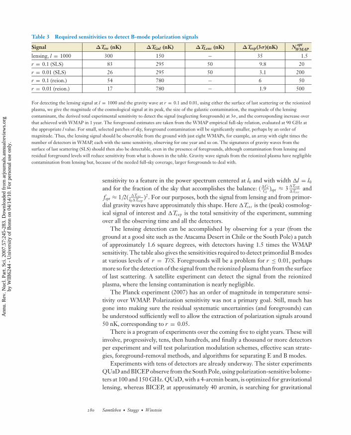
ANRV326-NS57-09 ARI 13 September 2007 7:27
Table 3 Required sensitivities to detect B-mode polarization signals
Signal ΔTcos (nK) ΔTGal (nK) ΔTLens (nK) ΔTexp(3σ)(nK) Nopt
WMAP
lensing, l = 1000 300 150 − 35 1.5r = 0.1 (SLS) 83 295 50 9.8 20r = 0.01 (SLS) 26 295 50 3.1 200r = 0.1 (reion.) 54 780 − 6 50r = 0.01 (reion.) 17 780 − 1.9 500
For detecting the lensing signal at l = 1000 and the gravity wave at r = 0.1 and 0.01, using either the surface of last scattering or the reionizedplasma, we give the magnitude of the cosmological signal at its peak, the size of the galaxtic contamination, the magnitude of the lensingcontaminant, the derived total experimental sensitivity to detect the signal (neglecting foregrounds) at 3σ , and the corresponding increase overthat achieved with WMAP in 1 year. The foreground estimates are taken from the WMAP empirical full-sky relation, evaluated at 90 GHz atthe appropriate l value. For small, selected patches of sky, foreground contamination will be significantly smaller, perhaps by an order ofmagnitude. Thus, the lensing signal should be observable from the ground with just eight WMAPs, for example, an array with eight times thenumber of detectors in WMAP, each with the same sensitivity, observing for one year and so on. The signatures of gravity waves from thesurface of last scattering (SLS) should then also be detectable, even in the presence of foregrounds, although contamination from lensing andresidual foreground levels will reduce sensitivity from what is shown in the table. Gravity wave signals from the reionized plasma have negligiblecontamination from lensing but, because of the needed full-sky coverage, larger foregrounds to deal with.
sensitivity to a feature in the power spectrum centered at l0 and with width �l = l0
and for the fraction of the sky that accomplishes the balance: ( �ClCl
)opt ≈ 3 �Texp�Tc o s
andfopt ≈ 1/2( �Tc o s
l0�Texp)2. For our purposes, both the signal from lensing and from primor-
dial gravity waves have approximately this shape. Here �Tc os is the (peak) cosmolog-ical signal of interest and �Texp is the total sensitivity of the experiment, summingover all the observing time and all the detectors.
The lensing detection can be accomplished by observing for a year (from theground at a good site such as the Atacama Desert in Chile or the South Pole) a patchof approximately 1.6 square degrees, with detectors having 1.5 times the WMAPsensitivity. The table also gives the sensitivities required to detect primordial B modesat various levels of r = T/S. Foregrounds will be a problem for r ≤ 0.01, perhapsmore so for the detection of the signal from the reionized plasma than from the surfaceof last scattering. A satellite experiment can detect the signal from the reionizedplasma, where the lensing contamination is nearly negligible.
The Planck experiment (2007) has an order of magnitude in temperature sensi-tivity over WMAP. Polarization sensitivity was not a primary goal. Still, much hasgone into making sure the residual systematic uncertainties (and foregrounds) canbe understood sufficiently well to allow the extraction of polarization signals around50 nK, corresponding to r = 0.05.
There is a program of experiments over the coming five to eight years. These willinvolve, progressively, tens, then hundreds, and finally a thousand or more detectorsper experiment and will test polarization modulation schemes, effective scan strate-gies, foreground-removal methods, and algorithms for separating E and B modes.
Experiments with tens of detectors are already underway. The sister experimentsQUaD and BICEP observe from the South Pole, using polarization-sensitive bolome-ters at 100 and 150 GHz. QUaD, with a 4-arcmin beam, is optimized for gravitationallensing, whereas BICEP, at approximately 40 arcmin, is searching for gravitational
280 Samtleben · Staggs ·Winstein
Ann
u. R
ev. N
ucl.
Part
. Sci
. 200
7.57
:245
-283
. Dow
nloa
ded
from
arj
ourn
als.
annu
alre
view
s.or
gby
WIB
6244
- U
nive
rsity
of
Bon
n on
04/
14/1
0. F
or p
erso
nal u
se o
nly.

ANRV326-NS57-09 ARI 13 September 2007 7:27
waves. MBI and its European analog BRAIN are testing the idea of using bolome-ters configured as an interferometer, and PAPPA is a balloon effort using waveguide-coupled bolometers from the Goddard Space Flight Center. These latter experimentshave beams in the range of 0.5◦ to 1◦.
Five initiatives at the level of hundreds of detectors have so far been put forth.Four use TES bolometers at 90, 150, and 220 GHz: CLOVER, the lone Europeaneffort, with an 8-arcmin beam; Polarbear, with a 4-arcmin beam; and EBEX andSPIDER, balloon-borne experiments with 8- and 20–70-arcmin beams, respectively(SPIDER and Polarbear will use antenna-coupled devices). The fifth uses coherentdetectors at 44 and 90 GHz: QUIET, initially with a 12-arcmin beam, observing fromthe Atacama Desert. All are dedicated ground-up polarization experiments that buildtheir own optical systems. The ACT and SPT groups, supported by the NationalScience Foundation, deploy very large telescopes to study both the cosmology ofclusters via the SZ effect and fine-scale temperature anisotropies, and will likelypropose follow-up polarimeters.
4.1. The Next Satellite Experiment
The reach of the next satellite experiment, termed CMBPOL as defined by the three-agency task force in the United States (36) and termed BPOL in Europe, is to detectthe signal from gravity waves limited only by astrophysical foregrounds. ExaminingFigure 6, we see that r = 0.01, and possibly lower values, can be reached. We shouldknow a great deal from the suborbital experiments well before the 2018 target launchdate. For studying polarization at large scales, where foregrounds pose their greatestchallenge, information from WMAP and Planck will be the most valuable.
5. CONCLUDING REMARKS
There is considerable promise for new, important discoveries from the CMB, onesthat can take us back to when the Universe’s temperature was between the GrandUnified Theory and Planck energy scales. This is particle physics, and while we hopeaccelerators will provide crucial evidence for, for example, the particle nature of darkmatter, exploring these scales seems out of their reach.
In some ways, cosmology has followed the path of particle physics: It has its Stan-dard Model, accounting for all confirmed phenomena. With no compelling theory,parameter values are not of crucial interest. We cannot predict the mass of the topquark, nor can we predict the primordial energy densities. Each discipline is checkingconsistency, as any discrepancies would be a hint of new physics.
The CMB field is not as mature as particle physics. It needs considerable detectordevelopment, even for current experiments. There is rapid progress, and overallsensitivity continues to increase. Foregrounds are certainly not sufficiently known orcharacterized. There is a great deal of competition in the CMB, like the early days ofparticle physics before the experiments grew so large that more than one or two teamsexploring the same topic worldwide was too costly. For the moment, this is good, aseach team brings something unique in terms of control of systematics, frequencies,
www.annualreviews.org • The CMB for Pedestrians 281
Ann
u. R
ev. N
ucl.
Part
. Sci
. 200
7.57
:245
-283
. Dow
nloa
ded
from
arj
ourn
als.
annu
alre
view
s.or
gby
WIB
6244
- U
nive
rsity
of
Bon
n on
04/
14/1
0. F
or p
erso
nal u
se o
nly.

ANRV326-NS57-09 ARI 13 September 2007 7:27
regions of the sky scanned, and detection technology. However, there is a differencein the way results are reported in the two fields. In the CMB field, typically almostnothing is said about an experiment between when it is funded and when it publishes.Here publishing means that results are announced, multiple papers are submitted andcirculated, and often there is a full data release, including not only of raw data andintermediate data products but sometimes support for others to repeat or extend theanalyses. The positives of this tradition are obvious. However, one negative is thatone does not learn the problems an experiment is facing in a timely manner. Thereis a degree of secrecy among CMB scientists.
There are other differences. CMB teams frequently engage theorists to performthe final analysis that yields the cosmological significance of the data. Sophisticatedanalysis techniques are being developed by a set of scientists and their students whodo not work with detectors but do generate a growing literature. There are as yetno standardized analysis techniques; effectively each new experiment invents its own.The days appear to be over where the group of scientists that design, build, and operatean experiment can, by themselves, do the full scientific analysis. Another distinction isthat there is no one body looking over the field or advising the funding agencies, andprivate funds sometimes have a major impact. Nearly all CMB scientists are workingon multiple projects, sometimes as many as four or five, holding that many grants.More time is spent writing proposals and reports and arranging support for juniorscientists, for whom there is little funding outside of project funds. This is certainlynot the optimum way to fund such an exciting and promising field.
DISCLOSURE STATEMENT
The authors have a CMB polarization experiment of their own.
ACKNOWLEDGMENTS
The authors have enjoyed many productive conversations with colleagues at theirinstitutions in the course of preparing this review. The authors are particularlygrateful for helpful comments from Norman Jarosik, Bernd Klein, Laura La Porta,and Kendrick Smith. We also wish to acknowledge our collaborators in QUIETand CAPMAP for frequent discussions of relevant issues. This work was partiallysupported by grants from the National Science Foundation: PHY-0355328, PHY-0551142, and ASTR/AST-0506648.
LITERATURE CITED
1. Kamionkowski M, Kosowsky A. Annu. Rev. Nucl. Part. Sci. 49:77 (1999)2. Dodelson S. Modern Cosmology. Acad. Press (2003)3. Penzias AA, Wilson RW. Astrophys. J. 142:419 (1965)4. Partridge RB. 3K: The Cosmic Microwave Background Radiation. Cambridge, NY:
Cambridge Univ. Press (1995)5. Fixsen DJ, et al. Astrophys. J. 483:586 (1996)
282 Samtleben · Staggs ·Winstein
Ann
u. R
ev. N
ucl.
Part
. Sci
. 200
7.57
:245
-283
. Dow
nloa
ded
from
arj
ourn
als.
annu
alre
view
s.or
gby
WIB
6244
- U
nive
rsity
of
Bon
n on
04/
14/1
0. F
or p
erso
nal u
se o
nly.

ANRV326-NS57-09 ARI 13 September 2007 7:27
6. Feng JL, Rajaraman A, Takayama F. Phys. Rev. D 68:063504 (2003)7. Smoot GF, et al. Astrophys. J. 396:1 (1992)8. Hinshaw G, et al. Astrophys. J. In press (2007)9. Bock J, et al. astro-ph/0604101 (2006)
10. Smith TL, Kamionkowski M, Cooray A. Phys. Rev. D 73(2):023504 (2006)11. Spergel DN, et al. Astrophys. J. In press (2007)12. Page L, et al. Astrophys. J. Suppl. 148:233 (2003)13. Readhead ACS, et al. Science 306:836 (2004)14. MacTavish CJ, et al. Astrophys. J. 647:799 (2006)15. Tegmark M, et al. Phys. Rev. D 69:103501 (2004)16. Hu W, Sugiyama N. Phys. Rev. D 51:2599 (1995)17. Eisenstein DJ, et al. Astrophys. J. 633:560 (2005)18. Bennett CL, et al. Astrophys. J. Suppl. 148:97 (2003)19. Page L, et al. Astrophys. J. In press (2007)20. La Porta L, Burigana C, Reich W, Reich P. Astron. Astrophys. 455(2):L9 (2006)21. Carretti E, Bernardi G, Cortiglioni S. MNRAS 373:93 (2006)22. Hanany S, Rosenkranz P. New Astron. Rev. 47(11–12):1159 (2003)23. Pietranera L, et al. MNRAS. In press (2007)24. Finkbeiner DP, Davis M, Schlegel DJ. Astrophys. J. 524:867 (1999)25. Vaillancourt JE. Eur. Astron. Soc. Publ. Ser. 23:147 (2007)26. Benoit A, et al. Astron. Astrophys. 424:571 (2004)27. Ponthieu N, et al. Astron. Astrophys. 444:327 (2005)28. Huffenberger KM, Eriksen HK, Hansen FK. Astrophys. J. 651:81 (2006)29. Stivoli F, Baccigalupi C, Maino D, Stompor R. MNRAS 372:615 (2006)30. Verde L, Peiris HV, Jimenez R. J. Cosmol. Astropart. Phys. 1:19 (2006)31. Barkats D, et al. Astrophys. J. Suppl. 159(1):1 (2005)32. Ryle M. Proc. R. Soc. A 211:351 (1952)33. Zmuidzinas J. Appl. Optics 42:4989 (2003)34. Mather JC. Appl. Optics 21:1125 (1982)35. Tegmark M. Phys. Rev. D 56:4514 (1997)36. Smith K. New Astron. Rev. 50(11–12):1025 (2006)37. Crawford T. astro-ph/0702608 (2007)38. Couchout F, et al. CMB and physics of the early universe. http://pos.sissa.it/
cgi-bin/reader/conf.cgi?confid=27 (2006)39. Bond JR, Jaffe AH, Knox L. Astrophys. J. 533:19 (2000)40. Hivon E, et al. Astrophys. J. 567:2 (2002)
www.annualreviews.org • The CMB for Pedestrians 283
Ann
u. R
ev. N
ucl.
Part
. Sci
. 200
7.57
:245
-283
. Dow
nloa
ded
from
arj
ourn
als.
annu
alre
view
s.or
gby
WIB
6244
- U
nive
rsity
of
Bon
n on
04/
14/1
0. F
or p
erso
nal u
se o
nly.


![28. Cosmic Microwave Backgroundpdg.lbl.gov/.../rpp2019-rev-cosmic-microwave-background.pdf · 2019. 12. 6. · cosmic microwave background (CMB), discovered in 1965 [1]. The spectrum](https://img.pdfslide.net/doc/110x75/6143c67b6b2ee0265c02424a/28-cosmic-microwave-2019-12-6-cosmic-microwave-background-cmb-discovered.jpg)