HAL Id: halshs-01023807https://halshs.archives-ouvertes.fr/halshs-01023807v3

Preprint submitted on 14 Dec 2015

HAL is a multi-disciplinary open accessarchive for the deposit and dissemination of sci-entific research documents, whether they are pub-lished or not. The documents may come fromteaching and research institutions in France orabroad, or from public or private research centers.

L’archive ouverte pluridisciplinaire HAL, estdestinée au dépôt et à la diffusion de documentsscientifiques de niveau recherche, publiés ou non,émanant des établissements d’enseignement et derecherche français ou étrangers, des laboratoirespublics ou privés.

The Counterparty Risk Exposure of ETF InvestorsChristophe Hurlin, Gregoire Iseli, Christophe Pérignon, Stanley Yeung

To cite this version:Christophe Hurlin, Gregoire Iseli, Christophe Pérignon, Stanley Yeung. The Counterparty Risk Ex-posure of ETF Investors. 2014. �halshs-01023807v3�

The Counterparty Risk Exposure of ETF Investors

Christophe Hurlin, Grégoire Iseli, Christophe Pérignon, and Stanley Yeung �

November 25, 2015

Abstract

As most Exchange-Traded Funds (ETFs) engage in securities lending or are based on

total return swaps, they expose their investors to counterparty risk. In this paper,

we estimate empirically such risk exposures for a sample of physical and swap-based

funds. We �nd that counterparty risk exposure is higher for swap-based ETFs, but

that investors are compensated for bearing this risk. Using a di¤erence-in-di¤erences

speci�cation, we uncover that ETF �ows respond signi�cantly to changes in counter-

party risk. Finally, we show that switching to an optimal collateral portfolio leads to

substantial reduction in counterparty risk exposure.

Keywords: Asset management, collateral, derivatives, regulatory arbitrage, systemic risk.

JEL classi�cation: G20, G23

�Hurlin is at the University of Orléans, France; Iseli, Pérignon and Yeung are at HEC Paris, France.Email and phone of corresponding author: perignon@hec.fr, +33 139 67 94 11. We are grateful to TonyBerrada, Hortense Bioy, Caitlin Dannhauser, Thierry Foucault, Laurent Frésard, Francesco Franzoni, DenisGromb, Johan Hombert, Hugues Langlois, Arnaud Llinas, Denis Panel, Manooj Mistry, Je¤rey Ponti¤,Sébastien Ringuedé, Richard Roll, Thierry Roncalli, Ioanid Rosu, Jean-David Sigaux, Guillaume Vuillemey,to seminar participants at the Autorité de Contrôle Prudentiel et de Résolution (ACPR), BNP-Paribas,the European Securities and Markets Authority (ESMA), Institut Louis Bachelier, Lyxor, University ofGeneva, University of Neuchatel, and University of Orléans, and to participants at the 2015 EuropeanFinancial Management Association Meeting, 2015 French Finance Association Meeting, and 2015 AnnualWorkshop of the Dauphine-Amundi Chair in Asset Management for their comments. We are grateful to theChair ACPR/Risk Foundation: Regulation and Systemic Risk and to the Amundi-Dauphine Chair in AssetManagement for supporting our research.

1

�If you buy a Lyxor product, you�re an unsecured creditor of SocGen.�

Laurence D. Fink, CEO of BlackRock (the leading physical ETF issuer), Bloomberg (2011).

1 Introduction

With their low fees and ability to provide exposure to a variety of asset classes, exchange-

traded funds (ETFs) have become popular investment vehicles among individual and insti-

tutional investors alike. The global ETF industry reached a total of $3 trillion in assets

under management (AUM) in 2015-Q3 and experienced an average growth of 28% per year

for the past �fteen years (BlackRock, 2015).

ETFs come in two types. In a physical ETF, investors�money is directly invested in the

index constituents in order to replicate the index return. Di¤erently in a synthetic ETF,

the fund issuer enters into a total return swap with a �nancial institution which promises to

deliver the performance of the index to the fund (Ramaswamy, 2011). An industry survey

by Vanguard (2013) indicates that 17% of the ETFs in the US are synthetic compared to

69% in Europe.1 Furthermore, most leveraged and inverse ETFs traded in the world are

based on synthetic replications (Tang and Xu, 2013).

In this paper, we empirically estimate the counterparty risk exposure of ETF investors.

Indeed, physical ETF issuers generate extra revenues by engaging in securities lending

(Blocher and Whaley, 2015). Hence, there is a possibility that the securities on loan will

not be returned in due time. Furthermore, for synthetic ETFs, there is a risk that the total

1Synthetic ETFs are less common in the US because (1) swaps between a¢ liated parties are not permittedunder the Investment Company Act of 1940 and (2) swap income faces a higher tax rate than capitalgains incurred by transacting in the underlying securities. Other examples of investment vehicles builton derivatives include the retail structured products studied in Célérier and Vallée (2015). For papers onderivative usage by mutual funds and hedge funds, see Koski and Ponti¤ (1999) and Chen (2011).

2

return swap counterparty will fail to deliver the index return. In order to mitigate counter-

party risk, both securities lending positions and swaps must be collateralized. Recently, the

Financial Stability Board (2011) and the International Monetary Fund (2011) warned about

potential �nancial stability issues that may arise from synthetic ETFs. The latter were ac-

cused of being poorly collateralized and allowing banks to engage in regulatory arbitrage by

using risky assets as collateral.

We de�ne counterparty risk of ETFs as the risk that the value of the collateral falls

below the Net Asset Value (NAV) of the fund when the fund counterparty is in default.

To quantify this risk empirically, we analyze the composition of the collateral portfolios of

a sample of physical and synthetic ETFs managed by two leading ETF issuers, BlackRock

and db X-trackers. For each fund, we know the exact composition of the collateral portfolio

at the end of each week. This is to the best of our knowledge the �rst time that such a

dataset is used in an academic study. The high granularity of our data allows us to study

empirically the counterparty risk of ETFs for various asset classes, regional exposures, and

types of replication.

Our analysis of the collateral portfolios of synthetic funds reveals several important fea-

tures of collateral management. First, collateral portfolios are well diversi�ed and their value

often exceeds the NAV of the fund (the average collateralization is 108.4%). Second, there

is a good �t between the asset exposure of the fund (e.g. equity or �xed income) and the

collateral used to secure the swap. This feature is important given the fact that in the case

of a default of the swap counterparty, the asset manager would need to sell collateral to meet

redemptions from investors. Third, ETF collateral is of high quality (e.g. equities from large

3

�rms and highly-rated bonds).

We quantify the counterparty risk exposure of investors using the expected magnitude

of the collateral shortfall. This measure is computed conditionally on the default of the

fund counterparty. When contrasting the level of counterparty risk exposure of investors in

synthetic and physical ETFs, we �nd that counterparty risk exposure is higher for synthetic

funds but that investors are compensated for bearing this risk through lower tracking errors

and similar or lower fees. We also show that ETF investors do care about counterparty risk.

Indeed, using a di¤erence-in-di¤erences approach, we �nd that there are more out�ows from

synthetic ETFs after an increase in counterparty risk.

In a �nal step, we theoretically show how to design an optimal collateral portfolio that

aims to minimize the counterparty risk exposure of ETF investors. The composition of the

optimal collateral portfolio is obtained by maximizing the investors�expected utility, de�ned

as a decreasing function of the collateral shortfall. Using our sample of ETFs, we �nd that,

on average, switching from an actual collateral portfolio to an optimal collateral portfolio

would lead to a 23% reduction in counterparty risk exposure.

Our paper contributes to the growing literature on the potential �nancial stability issues

arising from ETFs.2 Malamud (2015) derives a dynamic general equilibrium model of ETFs

that accounts for the share creation/redemption mechanism conducted by "Authorized Par-

ticipants" in the primary market. Contrary to the prevailing view among regulators, he

shows that ETF trading does not always increase the volatility of the underlying asset. Fur-

2For additional evidence on the link between asset management and �nancial stability, see Coval andSta¤ord (2007), Mitchell, Pedersen and Pulvino (2007), Boyson, Stahel and Stulz (2010), Chen, Goldsteinand Jiang (2010), Jotikasthira, Lundblad and Ramadorai (2012), Kacperczyk and Schnabl (2013), andSchmidt, Timmermann and Wermers (2014).

4

thermore, in this model, introducing new ETFs can reduce co-movement in the returns and

improve the liquidity of the underlying securities. There are a large number of empirical

papers focusing on one particular e¤ect of ETF trading. Ben-David, Franzoni and Moussawi

(2014) empirically show that ETF ownership increases stock volatility. Their identi�cation

strategy is based on the mechanical variation in ETF ownership due to stocks switching

from the Russell 1000 index to the Russel 2000 index; hence attracting more holdings from

index funds. Da and Shive (2013) �nd a strong relation between measures of ETF activity

and return comovement among stocks. Dannhauser (2014) shows that corporate bond ETFs

have an insigni�cant or negative impact on the liquidity of constituent bonds (see Hamm,

2014, for evidence on equity funds).

Focusing on the real e¤ects of ETF rebalancing activities, Bessembinder et al. (2015)

report no evidence of predatory trading around the time of the Crude Oil ETFs rolls of

crude oil futures (for a broader analysis of the e¤ects of predictable institutional orders,

see Bessembinder, 2015). Focusing on leveraged and inverse funds, Bai, Bond and Hatch

(2012) �nd that late-day leveraged ETF rebalancing activity signi�cantly moves the price of

constituent stocks (see also Shum et al., 2014, Tuzun, 2014, Ivanov and Lenkey, 2014).

Unlike previous academic studies, we do not focus on the interplay between the ETFs and

the assets they track. Instead, our study considers a source of risk that has been neglected so

far in the academic literature: the counterparty risk of ETFs. We make several contributions

to the existing literature. To the best of our knowledge, our study is the �rst attempt to

assess empirically the quality of the collateral for a large and representative sample of ETFs.

Our second contribution is to empirically compare the counterparty risk exposures of ETF

5

investors and identify the types of funds that expose the most their investors to this risk. We

also analyze how investors react to changes in the level of counterparty risk they are exposed

to. Finally, we contrast actual and optimal collateral portfolios, which lead by design to the

lowest possible level of counterparty risk. We believe that this is the �rst attempt to derive

optimal allocation rules for collateral portfolios, which is a topic of growing importance given

the emphasis put on collateral by the recent �nancial regulatory reform (Dodd Franck in the

US and EMIR in Europe).

The rest of our study is structured as follows. In Section 2, we explain why and how

ETFs can expose their investors to counterparty risk. Section 3 presents our collateral data.

In Section 4, we empirically estimate counterparty risk exposures for our sample funds and

test whether investors care about this source of risk. In Section 5, we show how to build an

optimal collateral portfolio that aims to minimize investors�counterparty risk exposure. We

conclude our study in Section 6.

2 Sources of Counterparty Risk in ETFs

2.1 Physical Model

Physical ETFs track their target index by holding all, or a representative sample, of the

underlying securities that make up the index (see Figure 1, Panel A). For example, if you

invest in an S&P 500 ETF, you own each of the 500 securities represented in the S&P 500

Index, or some subset of them. Almost all ETF issuers have the provision in their prospectus

for loaning out their stock temporarily for revenue. Over the period 2009-2013, Blocher and

Whaley (2015) estimate that the revenues generated by ETFs through securities lending are

comparable in size with management fees.

6

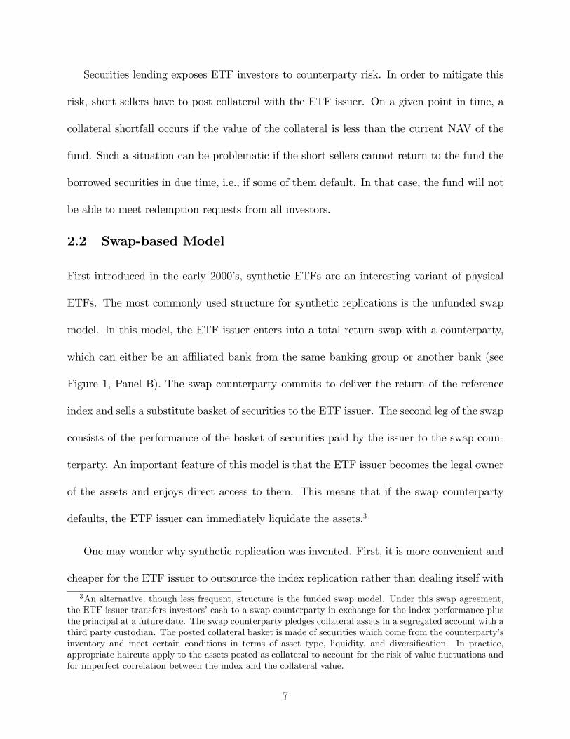
Securities lending exposes ETF investors to counterparty risk. In order to mitigate this

risk, short sellers have to post collateral with the ETF issuer. On a given point in time, a

collateral shortfall occurs if the value of the collateral is less than the current NAV of the

fund. Such a situation can be problematic if the short sellers cannot return to the fund the

borrowed securities in due time, i.e., if some of them default. In that case, the fund will not

be able to meet redemption requests from all investors.

2.2 Swap-based Model

First introduced in the early 2000�s, synthetic ETFs are an interesting variant of physical

ETFs. The most commonly used structure for synthetic replications is the unfunded swap

model. In this model, the ETF issuer enters into a total return swap with a counterparty,

which can either be an a¢ liated bank from the same banking group or another bank (see

Figure 1, Panel B). The swap counterparty commits to deliver the return of the reference

index and sells a substitute basket of securities to the ETF issuer. The second leg of the swap

consists of the performance of the basket of securities paid by the issuer to the swap coun-

terparty. An important feature of this model is that the ETF issuer becomes the legal owner

of the assets and enjoys direct access to them. This means that if the swap counterparty

defaults, the ETF issuer can immediately liquidate the assets.3

One may wonder why synthetic replication was invented. First, it is more convenient and

cheaper for the ETF issuer to outsource the index replication rather than dealing itself with

3An alternative, though less frequent, structure is the funded swap model. Under this swap agreement,the ETF issuer transfers investors�cash to a swap counterparty in exchange for the index performance plusthe principal at a future date. The swap counterparty pledges collateral assets in a segregated account with athird party custodian. The posted collateral basket is made of securities which come from the counterparty�sinventory and meet certain conditions in terms of asset type, liquidity, and diversi�cation. In practice,appropriate haircuts apply to the assets posted as collateral to account for the risk of value �uctuations andfor imperfect correlation between the index and the collateral value.

7

dividend �ows, corporate events, changes in index composition, or storage for commodities.4

Second, swap-based replications limit investors�exposure to tracking error risk (see Section

4.3 below). Third, synthetic replication greatly simpli�es the tracking of illiquid assets as

well as the issuance of inverse funds. Fourth, these swaps constitute a major source of

funding for �nancial institutions and lead to synergies and cost saving with their investment

banks which maintain large inventories of equities and bonds. Finally, they may also allow

the banks that act as swap counterparties to reduce their regulatory capital by posting high

risk-weight securities as collateral.

The counterparty exposure of the issuer, or swap value, is measured as the di¤erence

between the NAV and the value of the substitute basket (per share) used as collateral. The

swap is marked to market at the end of each day and reset whenever the counterparty

exposure exceeds a given threshold expressed as a percentage of the NAV. It is worth noting

that synthetic-ETF investors are particularly exposed to counterparty risk in the case of an

inverse ETF. In this case, the bank that acts as the swap counterparty must deliver a return

that increases with the severity of a stock market crash, i.e., when the default probability of

the bank is particularly high and when the value of the collateral is particularly low. This

is clearly a case of wrong-way risk.

3 Data and Descriptive Statistics

3.1 Types of Funds

Our empirical analysis is based on a sample of 218 ETFs with $115.4 billion combined

AUM. An attractive feature of our sample is that it includes both synthetic and physical

4An industry survey by Morningstar (2012) indicates that swap fees are extremely low and can even bezero if the swap is entered with an investment bank from the same banking group.

8

ETFs.5 We see in Table 1 that the 164 synthetic ETFs have combined AUM of $37.9 billion,

which is approximately 30% of the total AUM of all synthetic ETFs in Europe (Vanguard,

2013). The data on synthetic funds have been retrieved from the db X-trackers website

(www.etf.db.com). Our dataset includes both synthetic ETFs based on funded swaps and

on unfunded swaps and they account for quite similar AUM ($20.1 billion vs. $17.8 billion).

It is also important to notice that a signi�cant fraction of the synthetic funds (30 funds and

5.1% of AUM) are inverse funds that deliver the inverse performance of an index.

In terms of asset class, the majority of the synthetic ETFs are equity funds (74.5%

of AUM). Besides equity, other funds allow investors to be exposed to government bonds

(11%), treasuries and commercial papers (6.6%), commodities (3.8%), hedge funds (2.2%),

credit (0.7%), corporate bonds (0.6%), and currencies (0.3%). In that sense, our sample is

representative of the entire ETF industry as the share of equity ETFs is around 70% and

that of �xed-income funds, commodity funds, and currency funds are 18%, 11%, and 0.3%,

respectively (BlackRock, 2012).

As shown in Table 1, the sample of physical ETFs is more than twice as large as the

synthetic one ($77.5 billion vs. $37.9 billion of AUM). The data on physical ETFs have

been collected from the iShares website (www.ishares.com). Similar to the synthetic ETF

dataset, physical funds mainly track equity indices (around 70% of AUM) and government

bond indices (around 10%). However, corporate bond funds represent close to 20% of the

aggregate AUM of physical funds. Furthermore, the physical fund sample is primarily made

of funds that track European indices (47.6% of AUM) and world indices (24.9%).

5We only consider funds for which we have a complete history of weekly collateral data (see Section 3.2)and at least one year of data for the ETF price and its index.

9

3.2 Collateral Portfolios

Allegations were recently made about the poor collateralization of ETFs. For instance, the

Financial Stability Board (2011, page 4) states: "the synthetic ETF creation process may be

driven by the possibility for the bank to raise funding against an illiquid portfolio [...] the

collateral basket for a S&P 500 synthetic ETF could be less liquid equities or low or unrated

corporate bonds in an unrelated market."

To formally test for the validity of these allegations, we collect for each sample fund the

composition and the value of its collateral portfolio with a weekly frequency between July 5,

2012 and November 29, 2012. The collateral data have been retrieved from the db X-trackers

and iShares websites but because the websites keep no historical data, we had to download

the collateral data for each fund, every week over our sample period. Then for each security

used as collateral, we obtain its historical daily prices from Datastream.6

In Table 2, we see that the aggregate size of all collateral portfolios is equal to $40.9 billion

for synthetic ETFs, which indicates that, on average, the funds included in our analysis are

overcollateralized (AUM is $37.9 billion). For a given synthetic fund, the value-weighted

average level of collateralization is 108.4%. In total, there are 3,299 di¤erent securities that

are used as collateral in the synthetic ETF sample, which leads to 81 collateral securities per

fund on average. We notice that the number of securities is much higher for equity (around

100 securities per fund) than for �xed-income funds (10 to 20 securities per fund).

The situation is fairly di¤erent for physical funds as only a fraction of the AUM needs

to be collateralized, namely the part that is loaned out. On any given day, a typical fund

6For bonds, we use the returns of the bond index that best matches the attributes of the bonds: its type(sovereign vs. corporate), country, rating, and maturity.

10

lends 7.5% of its AUM on the securities lending market but the maximum value in our

sample is 94.3% (the average of the maximum lending ratios is 18.5%). We also notice

that securities lending is more important in government bond funds (17.2%) than in equity

funds (6.5%) or corporate bond funds (6%). Similar to synthetic funds, physical funds are

also overcollateralized, with collateral value accounting for 109.1% of the values of the lent

securities. The level of diversi�cation of the collateral portfolios is even higher for physical

funds as they include hundreds of di¤erent collateralized securities (355 on average).

3.3 Match between Index and Collateral

A criticism addressed to ETFs is the fact that the collateral may not be positively correlated

with the index tracked by the fund. Indeed, when the correlation is negative, the hedge

provided by the collateral is ine¢ cient: if the index return is large and positive when the

fund counterparty defaults, the value of the collateral shrinks and a collateral shortfall me-

chanically arises. To look at this issue empirically, we compare the index tracked by the

ETF and the securities included in the collateral portfolio. In Panel A of Table 3, we notice

that for synthetic funds most of the collateral is made of equities: when measured in value,

equities account for around 75% of the collateral vs. 20% for government bonds and 5% for

corporate bonds. An important �nding in this panel is that there is a good match between

the index tracked and the collateral as 92.5% of equity ETFs are backed with equity and

96.5% of government bonds ETFs are collateralized with government bonds. The match is

also pretty good for funds that track European indices as 71.8% of the collateral are made

of securities issued by European �rms.7

7To understand the predominant role played by European collateral, which we dub "collateral home bias",one needs to understand the origin of the pledged collateral. Indeed, these securities come from the books

11

Our empirical results also have some implications for the debate on the alleged regu-

latory arbitrage of the banks that act as swap counterparties. As previously mentioned,

international agencies claim that banks primarily post assets that require more regulatory

capital, such as less liquid and more risky assets. The high fraction of equities and the pres-

ence of corporate bonds in collateral portfolios are suggestive of banks strategically using

collateral to minimize their regulatory capital as both equities and corporate bonds are high

risk-weighted asset classes.

The situation for physical ETFs in Panel B of Table 3 contrasts sharply with the one of

synthetic ETFs. Indeed, iShares mainly receives equities as collateral as they account for

97.2% of the posted collateral. As a result, the match between the index and the collateral

is very high for equity funds (98.8%) but much lower for government bond funds (9.9%)

and corporate bond funds (0%). Another strong feature of the collateral used by iShares

is the predominant role played by equities issued by Asian (almost exclusively Japanese)

companies, which account for more than half of the value of the posted collateral.

To get a better sense of the type of securities used as collateral, we conduct in the

Appendix an in-depth analysis of all collateralized equities (Table A1) and of all collateralized

bonds (Table A2). Because they attract most critics from regulators, we focus on synthetic

ETFs. The main �ndings about collateralized equities are that (1) they are mainly issued

by large, European, non-�nancial �rms; (2) they exhibit good liquidity on average, with low

bid-ask spreads and high trading volume; (3) they have a higher beta with respect to the

ETF than with respect to the stock return of Deutsche Bank, which is the swap counterparty

of the swap counterparty, typically a large �nancial institution. In our sample, the swap counterparty isDeutsche Bank and as a result, its books predominantly include securities issued by local �rms held forinvestment purposes, market making, or other intermediation activities.

12

for all ETFs. As for collateralized bonds, we �nd that (1) they predominantly come from

European issuers (88.3%); (2) two-third of the bonds have a AAA rating; (3) the interest

rate duration of the collateral portfolios matches well with the duration of the �xed-income

index tracked by the fund.

Now that we have documented the level and nature of ETF collateral, we are going to

estimate in the following section counterparty risk exposures and test whether investors care

about this source of risk.

4 Counterparty Risk Analysis

4.1 Theoretical Framework

In any ETF structure, the counterparty risk borne by the ETF issuer, and ultimately the

investors, is equivalent to the risk that the ETF is not fully collateralized at the point of

default by the counterparty. If we denote by It, the NAV of the fund at time t, �t 2 [0; 1]

the fraction of the securities that are lent, Ct the value of the collateral per share, and h the

haircut, the collateral shortfall, denoted �t, corresponds to:

�t = �tIt � Ct (1� h) (1)

where �t 2 [0; 1] and h > 0 for physical ETFs, �t = 1 and h = 0 for unfunded-swap based

ETFs, and �t = 1 and h > 0 for funded-swap based ETFs. If �t > 0, additional collateral

is required to reach �tIt = Ct (1� h) (Morningstar, 2012). On a given date t, the one-day

ahead collateral shortfall �t+1 is de�ned as:

�t+1 = �tIt (1 + ri;t+1)� Ct (1� h) (1 + rc;t+1) (2)

13

where ri;t+1 and rc;t+1 denote the return of the NAV and the return of the collateral port-

folio, respectively. Given the information available at time t, the collateral shortfall �t+1 is

stochastic because the returns ri;t+1 and rc;t+1 are unknown.

By analogy with the credit risk literature, we consider both the default probability of the

counterparty and the loss given default. In our framework, the default probability concerns

the short seller (for physical ETFs) or the swap counterparty (for synthetic ETFs):

Pt+1 = Pr(Dt+1 = 1) (3)

where Dt+1 takes a value of one when the fund counterparty is in default and zero otherwise.

We note that the default probability does not depend on the collateralization of the fund

and can be estimated using standard techniques, such as structural models or CDS spreads.

The loss given default corresponds to the magnitude of the expected collateral shortfall:

St+1 = E (�t+1 j �t+1 > 0; Dt+1 = 1) (4)

where E denotes the conditional expectation on the information set Ft available at time t.

This metric, which corresponds to the collateral shortfall a fund is expected to experience

conditionally on the default of the counterparty, has several attractive features. First, given

its conditional nature, it only focuses on concerning situations where a counterparty default

and a collateral shortfall jointly occur. Second, it measures the changes in collateral value

when the counterparty is in default and, as such, captures the dependence between the

liquidity of the collateral and the creditworthiness of the counterparty. Third, it is a su¢ cient

risk measure if one aims to compare the counterparty risk exposure of funds having the same

counterparty, hence the same Pt+1. As this is our goal here, we focus in the rest of our

analysis on expected collateral shortfall.

14

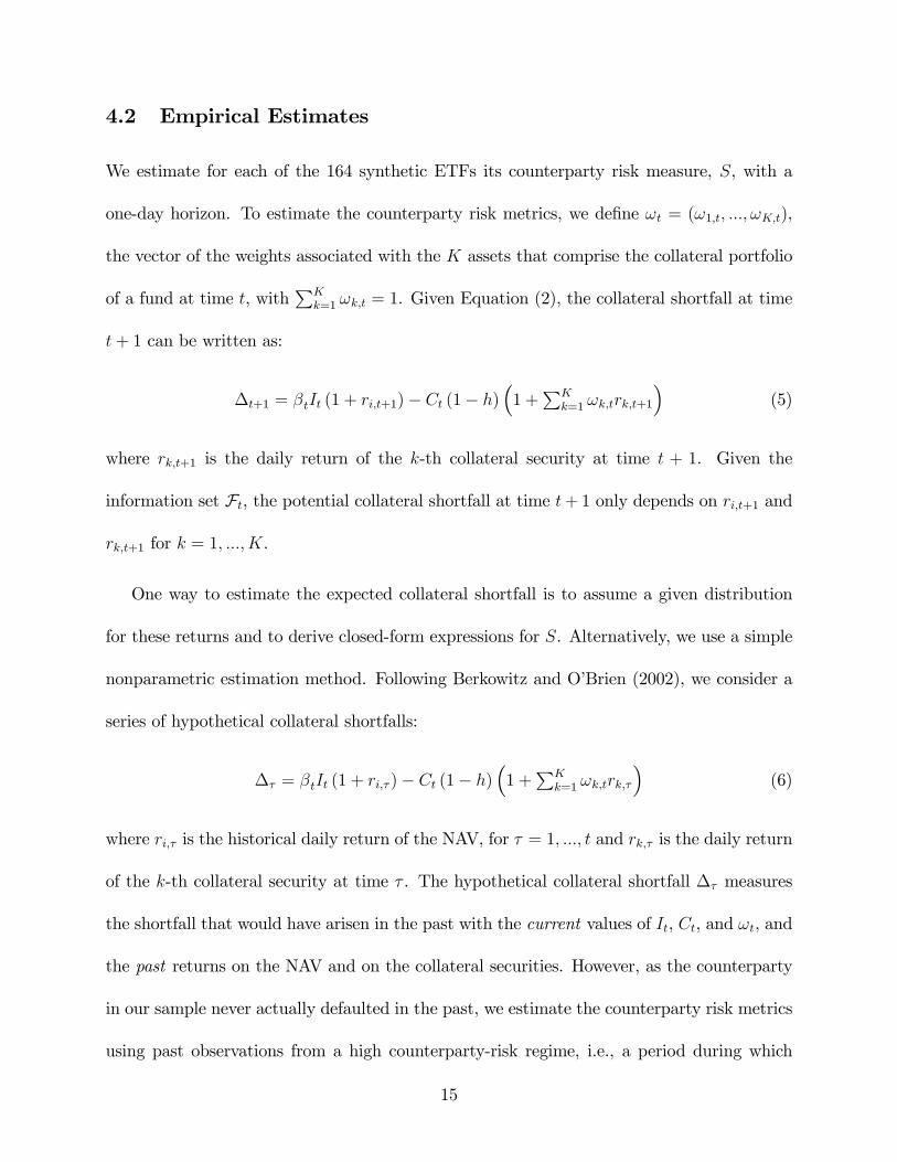
4.2 Empirical Estimates

We estimate for each of the 164 synthetic ETFs its counterparty risk measure, S, with a

one-day horizon. To estimate the counterparty risk metrics, we de�ne !t = (!1;t; :::; !K;t),

the vector of the weights associated with the K assets that comprise the collateral portfolio

of a fund at time t, withPK

k=1 !k;t = 1. Given Equation (2), the collateral shortfall at time

t+ 1 can be written as:

�t+1 = �tIt (1 + ri;t+1)� Ct (1� h)�1 +

PKk=1 !k;trk;t+1

�(5)

where rk;t+1 is the daily return of the k-th collateral security at time t + 1. Given the

information set Ft, the potential collateral shortfall at time t+ 1 only depends on ri;t+1 and

rk;t+1 for k = 1; :::; K.

One way to estimate the expected collateral shortfall is to assume a given distribution

for these returns and to derive closed-form expressions for S. Alternatively, we use a simple

nonparametric estimation method. Following Berkowitz and O�Brien (2002), we consider a

series of hypothetical collateral shortfalls:

�� = �tIt (1 + ri;� )� Ct (1� h)�1 +

PKk=1 !k;trk;�

�(6)

where ri;� is the historical daily return of the NAV, for � = 1; :::; t and rk;� is the daily return

of the k-th collateral security at time � . The hypothetical collateral shortfall �� measures

the shortfall that would have arisen in the past with the current values of It, Ct, and !t, and

the past returns on the NAV and on the collateral securities. However, as the counterparty

in our sample never actually defaulted in the past, we estimate the counterparty risk metrics

using past observations from a high counterparty-risk regime, i.e., a period during which

15

the counterparty experienced a sharp increase in its default probability. A nonparametric

estimator for the expected collateral shortfall is:

bSt+1 = Pt�=1�� � I (�� > 0)� I

�� 2 �

�Pt�=1 I (�� > 0)� I

�� 2 �

� (7)

where I (:) denotes the indicator function and � denotes a high-counterparty risk regime.

In our tests, the high counterparty-risk regime corresponds to the two-month period around

the bankruptcy of Lehman Brothers (September 1, 2008 - October 31, 2008). Over these

two months, the CDS-implied default probability of the swap counterparty, Deutsche Bank,

got multiplied by three, and its market capitalization dropped by 50%.

In Table 4, we display the distribution of the expected collateral shortfall, expressed

alternatively as a percentage of the NAV and in dollars, for all synthetic funds. For each

fund, the risk metrics are averaged across time. The main result in this �gure is that

counterparty risk exposure varies extensively across funds. While the expected shortfall

remains for most funds below 5% of the NAV, some of them exhibit an expected collateral

shortfall that corresponds to one third of their NAV.

As a comparison, we conduct a similar risk assessment for physical ETFs as they also

expose their investors to counterparty risk through securities lending. It is indeed possible

that the short sellers who borrow securities from the ETF issuer fail to return them in due

time. We see in Table 4 that the di¤erence in risk exposure is striking: counterparty risk

exposure is several orders of magnitude higher for synthetic ETF investors.

16

4.3 Trade-o¤ between Risk and Performance

We have seen that synthetic-ETFs�investors tend to be more exposed to counterparty risk

than physical-ETFs�investors. A natural question is whether the former investors are com-

pensated for bearing this additional risk. We answer this question by considering two im-

portant dimensions of an ETF: its costs and its tracking error. In particular, we formally

show that synthetic ETFs are as cheap or cheaper and display better performance (i.e., lower

tracking error) than physical ETFs.8 As a result, synthetic funds�investors are compensated

for bearing this additional risk by enjoying superior performance for the same price.

We conduct this test in two ways. In Panel A of Table 5, our unconditional tests reveal

no clear di¤erence between the fees charged by synthetic and physical funds.9 The average

fee for physical ETFs are 44 bps vs. 43 bps for synthetic ETFs. However, we �nd major

di¤erences in the tracking error of these funds: the average tracking error is 96 bps for

physical ETFs and 13 bps for synthetic ETFs. Another interesting result is the much higher

tracking error for funds that pay dividends (Distributing), which indicates that a major

source of tracking error for funds is the way dividends are handled and passed through to

investors.

In Panel B of Table 5, we complement these unconditional results by running multivariate

regressions for, in turn, fees and tracking errors. We �nd that the coe¢ cient associated with

the synthetic ETF�s dummy variable is negative and signi�cant for both the fees and the

tracking errors. Interestingly, we uncover that inverse funds tend to charge higher fees and

8We de�ne the tracking error as the annualized volatility of the di¤erence between the daily returns ofthe ETF and of the index.

9For an empirical analysis of the fees of active and passive (including ETFs) funds in the world, seeCremers et al. (2015).

17

funds that distribute dividends exhibit larger tracking errors. Di¤erently, tracking error

decreases with fund size.

4.4 Do ETF Investors Care about Counterparty Risk?

We now turn to testing whether ETF �ows are sensitive to changes in counterparty risk. We

envision that it could be the case for two reasons. First, a signi�cant fraction of all ETF

trading is made by institutional investors, which are perceived as sophisticated investors, and

they are able to withdraw funds quickly when they are not comfortable with the risk they

face. A recent example is the run on money market funds by institutional investors following

the bankruptcy of Lehman Brothers on September 15, 2008 (Schmidt, Timmermann and

Wermers, 2014). Second, the creditworthiness of the swap counterparty can be monitored in

real time in the CDS market.

While our fund �ow data start in 2008, we believe that most investors were not aware of

the counterparty risk concerns before 2011. Indeed, as mentioned in the introduction, the

debate on the counterparty risk of synthetic ETFs started during the �rst half of 2011 when

trenchant criticisms were made by international agencies and industry leaders (see quote of

Laurence D. Fink on page 2). To identify the exact timing, we searched for articles in the

�nancial press that include the words "synthetic ETF" (from the Factiva database) as well

as the number of queries on Google including the keywords "synthetic ETF" (from Google

Trends) between 2006 and 2015. Both proxies for market awareness remained at, or close

to, zero until 2011 and then jumped to almost 300 articles and to a Google Search Index of

100.

Our setting allows us to cleanly identify, using the di¤erence-in-di¤erences method, the

18

e¤ect of counterparty risk on synthetic ETF out�ows before and after 2011. Since we do not

observe �ows directly, we follow Frazzini and Lamont (2008) and Barber, Huang and Odean

(2015) and infer �ows from fund asset value and returns:

flowi;t = Ii;t �#outstanding_sharesi;t � Ii;t�1 �#outstanding_sharesi;t�1 � (1 + ri;t) (8)

where ri;t is the return of the NAV for fund i between time t � 1 and t. By doing so,

the performance of the fund is not taken into account as we only capture share redemptions

(out�ows) and share purchases (in�ows). Then, we run the following di¤erence-in-di¤erences

panel regression:

outflowi;t = �i + �1 �Riskt�1 � Postt + �2 �Riskt�1 + �3 � Postt + �4 � Perfi;t + "i;t (9)

where outflowi;t is either a dummy variable that takes a value of one if there is an out�ow

between t � 1 and t and zero otherwise (Probit model) or the log of the absolute out�ow

and zero if there is an in�ow (Tobit model). Riskt�1 is a dummy variable equal to one if

the CDS spread of the swap counterparty at time t � 1 is greater than the 75th percentile

of its distribution, Postt is a dummy variable that takes a value of one after June 2011, and

Perfi;t is the return of the index tracked by the fund a time t.

We estimate a Probit speci�cation of Equation (9) using monthly data on all synthetic

funds over the period August 2008-December 2013 and report the results in the �rst two

columns of Table 6. This di¤erence-in-di¤erences identi�cation allows us to compare syn-

thetic funds in high-risk states after June 2011 ("treated") to synthetic funds in low-risk

states as well as synthetic funds before June 2011 ("control"). Our main �nding is that

the estimated �1 parameter is positive and signi�cant. This suggests that once investors

19

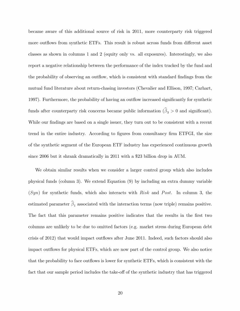
became aware of this additional source of risk in 2011, more counterparty risk triggered

more out�ows from synthetic ETFs. This result is robust across funds from di¤erent asset

classes as shown in columns 1 and 2 (equity only vs. all exposures). Interestingly, we also

report a negative relationship between the performance of the index tracked by the fund and

the probability of observing an out�ow, which is consistent with standard �ndings from the

mutual fund literature about return-chasing investors (Chevalier and Ellison, 1997; Carhart,

1997). Furthermore, the probability of having an out�ow increased signi�cantly for synthetic

funds after counterparty risk concerns became public information (b�3 > 0 and signi�cant).While our �ndings are based on a single issuer, they turn out to be consistent with a recent

trend in the entire industry. According to �gures from consultancy �rm ETFGI, the size

of the synthetic segment of the European ETF industry has experienced continuous growth

since 2006 but it shrank dramatically in 2011 with a $23 billion drop in AUM.

We obtain similar results when we consider a larger control group which also includes

physical funds (column 3). We extend Equation (9) by including an extra dummy variable

(Syn) for synthetic funds, which also interacts with Risk and Post. In column 3, the

estimated parameter b�1 associated with the interaction terms (now triple) remains positive.The fact that this parameter remains positive indicates that the results in the �rst two

columns are unlikely to be due to omitted factors (e.g. market stress during European debt

crisis of 2012) that would impact out�ows after June 2011. Indeed, such factors should also

impact out�ows for physical ETFs, which are now part of the control group. We also notice

that the probability to face out�ows is lower for synthetic ETFs, which is consistent with the

fact that our sample period includes the take-o¤ of the synthetic industry that has triggered

20

some important transfers from physical to synthetic funds. Another robustness check we

consider is to estimate the treatment e¤ect on the magnitude of the �ows. In column 4, we

estimate a Tobit model using the absolute out�ows as our dependent variable and the sign

of the coe¢ cients remain unchanged. Finally, we re-estimate our four speci�cations by using

the level of the CDS spread as the Risk variable. In all cases, we obtain qualitatively similar

(unreported) results.

5 Optimal Collateral Portfolio

5.1 De�nitions

In this study, we have extensively analyzed the size, composition, and performance of collat-

eral portfolios currently used in the ETF industry. In the last part of our analysis, we check

whether the performance of such collateral portfolios could be improved. To do so, we show

how to construct an optimal collateral portfolio that aims to protect ETF investors against

counterparty risk. With such a benchmark, we can empirically measure how much could be

gained by switching from an actual collateral portfolio to the optimal one. The process that

leads to the optimal collateral portfolio can be divided into three steps.

Step 1: Eligible securities The counterparty and the ETF issuer have to determine a set

of eligible securities. In practice, the securities pledged as collateral directly come from the

inventory of the counterparty, which includes securities held for investment purposes, market

making, underwriting, or other intermediation activities. When choosing the securities to be

pledged, the collateral provider might want to reduce its regulatory capital by transferring

21

high risk-weight securities and/or to minimize the opportunity cost of holding collateral.10

On the receiver side, only collateral with su¢ cient tradability will be admitted. This inter-

action between the provider and the receiver of collateral leads to the determination of a set

of K eligible securities that need to be allocated.

Step 2: Level of collaterization Both parties have to determine the level of collateral-

ization. At the end of day t, the value of the collateral portfolio Ct, adjusted by the haircut

h, is determined by the fraction �t of the NAV It which has to be collateralized and the

desired level of collateralization �:

Ct =��tIt(1� h) (10)

If � = 1, the fund is full collateralized at time t: When � > 1 the value of the collateral

portfolio, adjusted for haircut, is larger than the fraction �t of the NAV which has to be

collateralized. By substituting It from Equation (10) into Equation (11), we get:

�t+1 = Ct (1� h) 1� ��

+ri;t+1�

�KXk=1

!krk;t+1

!(11)

Step 3: Optimal composition of the collateral portfolio Given the eligible securities

and the level of collateralization on day t, the optimal composition of the collateral portfolio

is determined by choosing the weights ! = (!1; :::; !K) to maximize the investors�expected

utility on day t + 1, de�ned as a decreasing function of the collateral shortfall �t+1 (see

Appendix A), for �t+1 > 0.

10Such securities include those with relatively low fees on the securities lending market; those with relativelylow collateral value in the repo market (Bartolini et al., 2011); those that are not eligible as collateral forcentral-bank credit operations; and securities for which the demand is low on the secondary market (Brandtand Kavajecz, 2004).

22

De�nition 1 The optimal collateral portfolio !� = (!�1; :::; !�K)

0 at time t satis�es:

!� = argmax!2�t

E [u (��t+1)] (12)

subject to�! � 0e|! = 1

where u (:) is the utility function of the investors, �t denotes the set of all feasible portfolios

based on the K eligible securities, and e is the unit vector.

We impose ! to be non-negative since short positions in collateral would be nonsensical.

As usual, the sum of the portfolio weights is normalized to one. In practice, many other

types of constraints can be considered in the program.11

When the utility function is explicitly speci�ed, the optimal collateral portfolio can be

directly obtained by solving program (12) with analytical or numerical methods. There

is no particular constraint on the choice of the objective function, except that the program

should be well speci�ed and that there exists a unique optimal solution. Alternatively, in the

next subsection, we derive the optimal collateral portfolio through a mean-variance approach

(Markowitz, 1959), in which the investor�s expected utility is a function of the mean and the

variance of the collateral shortfall.

5.2 E¢ cient Frontier for Collateral Portfolios

A collateral portfolio is mean-variance e¢ cient if it minimizes the shortfall variance �2� (!) =

V (�t+1jDt+1 = 1) for a given mean �� (!) = E (�t+1jDt+1 = 1).

11One can prevent any issuer to account for more than a certain fraction of the collateral portfolio. Anotherconstraints can be added on the liquidity of the assets selected for the collateral portfolio or on the collateralportfolio itself. For instance, the optimal weights can be determined under the constraint that the liquidity ofthe optimal portfolio (measured according a particular liquidity risk measure) is larger than a lower bound.

23

De�nition 2 The e¢ cient frontier for collateral portfolios is given by all portfolios e! ( ) 2�t that are solutions of the following optimization program:

e! ( ) = argmin!2�t

�2� (!) (13)

subject to

8><>:�� (!) =

! � 0e|! = 1

where �t is the set of all eligible portfolios such that �� (!) � � and � is the mean short-

fall of the Global Minimum Variance Collateral Portfolio (GMVCP), i.e., the portfolio that

minimizes �2� (!).

Both moments �� (!) and �2� (!) can be expressed as functions of the moments of the

returns of the collateral securities and of the NAV. De�ne rt = (r1;t; :::; rK;t)| the K � 1

vector of returns of the collateral securities and zt = (ri;t=�; r|t )|, with:

E (zt+1jDt+1 = 1) =

0B@ �i(1;1)

�(K;1)

1CA (14)

�z = E ((zt+1 � E (zt+1)) (zt+1 � E (zt+1))|jDt+1 = 1) =

0B@ �2i(1;1)

�|i(1;K)

�i(K;1)

�(K;K)

1CA (15)

where �i and �2i respectively denote mean and variance of ri;t=�. Without loss of generality,

we assume that Ct (1� h) = 1 and express the program in Equation (13) as:

e! ( ) = argmin!2�t

1

2!|�! +

1

2�2i � !|�i (16)

subject to

8><>:�i � !|� = e ! � 0e|! = 1

with e = � (1� �) =�, for all � . The associated Lagrange function f (!; �1; �2; �3) is:f (!; �1; �2; �3) =

1

2!|�! +

1

2�2i � !|�i � �1 (e|! � 1)� �2 (!|�� �i + e )� �|3! (17)

24

with �1 > 0, �2 > 0 and �3;i � 0 for i = 1; :::; K. When the positivity constraints are not

binding (�3 = 0), the weights of the portfolios that belong to the e¢ cient frontier can be

expressed as a function of the weights of the Markowitz�s mean variance e¢ cient portfolios.12

We de�ne three scalars a, b, and c such that:

a = e|��1e b = e|��1� c = �|��1� (18)

where e is the unit vector.

Proposition 1 If �3 = 0, the weights of the e¢ cient portfolios are de�ned by:

e! ( ) = e!MV + ��1�i +

�ce| � b�|b2 � ac

���1�i�

�1e+

�a�| � be|b2 � ac

���1�i�

�1� (19)

where e!MV corresponds to the weights of the Markowitz�s mean-variance e¢ cient portfolios:

e!MV =

�b�i � be � cb2 � ac

���1e+

�b� a�i + ae b2 � ac

���1� (20)

and e = � (1� �) =�.The proof of Proposition 1 is provided in Appendix B. The e¢ cient weights depend

on � and �i, but they also depend on the vector of expected returns of the collateral

securities � and on the expected transformed return of the NAV �i � e . The latter can beviewed as a target for the expected return of the collateral portfolio, !|�. Notice that if

the collateral securities and the NAV are independent, �i = 0K�1, then the e¢ cient weights

simply correspond to the weights e!MV of the mean-variance portfolio with a target mean

�i � e .12When at least one asset k 2 f1; :::;Kg is excluded from the optimal portfolio, i.e., for which �3;k > 0

and !k = 0, there is no closed-form solution for the optimal constrained portfolio. However, the solutionof the program can be obtained by solving the unconstrained problem with an implied covariance matrix e�de�ned as a shrunk version of � that depends on the Lagrange coe¢ cients (Jagannathan and Ma, 2003).

25

Finally, the optimal portfolio !� is determined by choosing from the mean-variance e¢ -

cient portfolios e! ( ) for � � , the portfolio with the highest expected utility. An alternativesolution consists in choosing the portfolio that minimizes the non-parametric estimate of the

expected collateral shortfall bSt+1(Equation 7). The latter estimation strategy has the advan-tage of not imposing a particular utility function for the investors, neither any distributional

assumptions for the returns.

5.3 Actual vs. Optimal Collateral

We compare actual and optimal collateral portfolios for a sample of total return swaps

associated with some of the largest ETFs in our sample. The funds track respectively the

DAX index (equity), the Eurostoxx 50 index (equity), the iBoxx Global In�ation-Linked

index (Treasuries), and the iBoxx Sovereigns Eurozone index (Treasuries). On the last day

of our sample period (November 29, 2012), the assets under management (AUM) of these

funds range between $600 million for the iBoxx Sovereigns fund and $8.5 billion for the DAX

fund and the total return swaps associated are either fully collateralized or almost fully

collateralized.

The composition of the collateral portfolios is described in Panel A of Table 7. The actual

collateral portfolios of the sample ETFs include a total of 81 securities. The set of securities

used as collateral for these four ETFs includes 47 equities and 34 government bonds. The

number of posted securities in each portfolio ranges from 9 for the iBoxx Sovereigns Eurozone

swap to 31 to the DAX swap. Besides the 81 securities included in the four collateral

portfolios, we also know the identity of another 1,436 securities that are included, on the

same day, in the collateral portfolios of another 160 ETFs managed by db-X trackers. This

26

pool of K = 1; 517 (= 81 + 1,436) securities can be interpreted as the set �t of eligible

collateral securities (see Panel B). We note that the majority of the used collateral securities

are equities: 1,438 out of 1,517 vs. 62 government bonds and 27 corporate bonds.

For each sample swap, we estimate the e¢ cient collateral frontier and then pick the

optimal portfolio associated with the lowest expected collateral shortfall, which is estimated

non-parametrically. The covariance matrix � is estimated from asset returns observed during

a high counterparty-risk regime (September 1, 2008 - October 31, 2008). As the number of

collateral securities is larger than the number of dates in the high counterparty-risk regime,

the sample covariance matrix su¤ers from a small sample size problem and ends up being

singular. To alleviate this problem, we use the shrinkage estimator of the covariance matrix

�z proposed by Ledoit and Wolf (2003). The estimators of the expected returns �i and �

are de�ned by their empirical counterparts over the same period. The numerical solution for

the mean-variance frontier, with positivity constraints, is obtained using CVX, a package for

specifying and solving convex problems (Grant and Boyd, 2008).

Figure 2 displays the mean-variance e¢ cient frontier, along with the actual and optimal

collateral portfolios, for the swap on the Euro Stoxx 50 index. As the actual collateral

portfolio does not lie on the frontier, switching to the optimal portfolio would allow investors

to reduce both the mean and the variance of the collateral shortfall, hence reducing their

counterparty risk exposure.

Panel A of Table 7 compares the actual and optimal portfolios for the four ETFs. We

observe that the total number of securities included in the collateral portfolios are quire sim-

ilar (81 in the actual portfolios vs. 156 in the optimal portfolios) but that optimal portfolios

27

are more tilted towards equities than bonds. For each fund, the optimal number of securities

ranges between 36 and 71 securities, which is slightly larger than actual portfolios (between

9 and 31). However, as the optimization is based on a universe of around 1,500 securities,

these �ndings illustrate the relative concentration of the optimal collateral portfolios and

suggests that our approach leads to realistic portfolios. More importantly, optimal portfolios

are characterized by lower counterparty risk exposure: the expected collateral shortfall St+1

reduces by 29% for the equity ETFs (27.38% for the DAX and 30.39% for the Eurostock)

and by 17% for the bond ETFs (16.84% for the global in�ation index and 16.67% for the

sovereign index). This is evidence that active collateral management can greatly reduce the

counterparty risk associated with passive investment vehicles.

6 Conclusion

How safe are ETFs? We show in this paper that the answer to this question very much

depends on the collateral management policy of the fund issuers. We study the collateral

portfolios of ETFs that are based on swaps or engage in securities lending, hence exposing

their investors to counterparty risk. We �nd that funds tend to be overcollateralized and

that collateral mainly consists of equities and to a lesser extent highly rated bonds.

There is some heterogeneity in the level of counterparty risk exposure of ETF investors.

Risk exposure is shown to be higher for inverse ETFs which deliver the inverse perfor-

mance of the underlying index. We also �nd that counterparty risk exposure is higher for

synthetic ETFs but that investors are compensated for bearing this risk. Using a di¤erence-

in-di¤erences speci�cation, we show that ETF �ows respond signi�cantly to changes in coun-

terparty risk, which suggests that investors closely monitor their counterparty risk exposure.

28

Our �ndings on the importance of counterparty risk for ETF investors have been corrob-

orated by a recent change in business models for several leading asset managers. Given

investors�growing distrust in synthetic replication, Lyxor and db X-trackers, two long-time

proponents of synthetic ETFs, both decided to switch some of their largest funds to physical

replication (Financial Times, 2014).

29

References

[1] Bai, Q., S. A. Bond, and B. Hatch (2012) The Impact of Leveraged and Inverse ETFson Underlying Stock Returns, Working Paper.

[2] Barber, B. M., X. Huang, and T. Odean (2015) Which Risk Factors Matter to Investors?Evidence from Mutual Fund Flows, Working Paper.

[3] Bartolini, L., S. Hilton, S. Sundaresan, and C. Tonetti (2011) Collateral Values byAsset Class: Evidence from Primary Securities Dealers, Review of Financial Studies,24, 248-278.

[4] Ben-David, I. , F. A. Franzoni, and R. Moussawi (2014) Do ETFs Increase Volatility?,Working Paper.

[5] Berkowitz, J. and J. O�Brien (2002) How Accurate Are Value-at-Risk Models at Com-mercial Banks?, Journal of Finance, 57, 1093-1111.

[6] Bessembinder, H. (2015) Predictable ETF Order Flow and Market Quality, Journal ofTrading, 10, 17-23.

[7] Bessembinder, H., A. Carrion, L. Tuttle, and K. Venkataraman (2015) Liquidity, Re-siliency and Market Quality Around Predictable Trades: Theory and Evidence, Journalof Financial Economics, forthcoming.

[8] BlackRock (2012) ETP Landscape, November.

[9] BlackRock (2015) ETP Landscape, October.

[10] Blocher J. and R. E. Whaley (2015) Passive Investing: The Role of Securities Lending,Working Paper.

[11] Bloomberg (2011) BlackRock�s Fink Attacks Societe Generale Over ETF Risks, Novem-ber 17.

[12] Boyson, N., C. W. Stahel, and R. M. Stulz (2010) Hedge Fund Contagion and LiquidityShocks, Journal of Finance, 55, 1789-1816.

[13] Brandt, M. and K. Kavajecz (2004) Price Discovery in the U.S. Treasury Market: TheImpact of Order Flow and Liquidity on the Yield Curve, Journal of Finance, 59, 2623-2654.

[14] Carhart, M. (1997) On Persistence in Mutual Fund Performance, Journal of Finance,52, 57-82.

[15] Célérier C. and B. Vallée (2015) Catering to Investors through Products Complexity,Working Paper.

30

[16] Chen, Y. (2011) Derivatives Use and Risk Taking: Evidence from the Hedge FundIndustry, Journal of Financial and Quantitative Analysis, 46, 1073-1106.

[17] Chen, Q., I. Goldstein, and W. Jiang (2010) Payo¤ Complementarities and FinancialFragility: Evidence from Mutual Fund Out�ows, Journal of Financial Economics, 97,239-262.

[18] Chevalier, J. A. and G. D. Ellison (1997) Risk Taking by Mutual Funds as a Responseto Incentives, Journal of Political Economy, 105, 1167-1200.

[19] Coval, J. and E. Sta¤ord (2007) Asset Fire Sales (and Purchases) in Equity Markets,Journal of Financial Economics, 86, 479-512.

[20] Cremers, M., M. A. Ferreira, P. Matos, and L. Starks (2015) Indexing and Active FundManagement: International Evidence, Journal of Financial Economics, forthcoming.

[21] Da, Z. and S. Shive (2013) When the Bellwether Dances to Noise: Evidence fromExchange-Traded Funds, Working Paper.

[22] Dannhauser, C. D. (2014) The Equitization of the Corporate Bond Market: The Impactof ETFs on Bond Yields and Liquidity, Working Paper.

[23] Financial Stability Board (2011) Potential Financial Stability Issues Arising from RecentTrends in Exchange-Traded Funds (ETFs).

[24] Financial Times (2014) Lyxor Extends Physical ETF Push, June 17, 2014.

[25] Frazzini, A. and O. A. Lamont (2008) Dumb Money: Mutual Fund Flows and theCross-Section of Stock Returns, Journal of Financial Economics, 88, 299-322.

[26] Grant, M. and S. Boyd (2008) Graph implementations for nonsmooth convex programs,Recent Advances in Learning and Control, Ed. by V. Blondel, S. Boyd, and H. Kimura,Springer, 95-110.

[27] Hamm, S. J. W. (2014) The E¤ect of ETFs on Stock Liquidity, Working Paper.

[28] International Monetary Fund (2011) Global Financial Stability Report, 68-72.

[29] Ivanov, I. T., and S. L. Lenkey (2014) Are Concerns about Leveraged ETFs Overblown?,Working Paper, Board of Governors of the Federal Reserve System.

[30] Jagannathan, R. and T. Ma (2003) Risk Reduction in Large Portfolios: Why Imposingthe Wrong Constraints Helps, Journal of Finance, 58, 1651-1684.

[31] Jotikasthira, C., C. Lundblad, and T. Ramadorai (2012) Asset Fire Sales and Purchasesand the International Transmission of Funding Shocks, Journal of Finance, 67, 2015-2050.

31

[32] Kacperczyk, M. T. and P. Schnabl (2013) How Safe are MoneyMarket Funds?, QuarterlyJournal of Economics, 128, 1073-1122.

[33] Koski, J. L. and J. Ponti¤ (1999) How Are Derivatives Used? Evidence from the MutualFund Industry, Journal of Finance, 54, 791-816.

[34] Ledoit, O. and M. Wolf (2003) Improved Estimation of the Covariance Matrix of StockReturns with an Application to Portfolio Selection, Journal of Empirical Finance, 10,603-621.

[35] Malamud, S. (2015) A Dynamic Equilibrium Model of ETFs, Working Paper.

[36] Markowitz, H. M. (1959) Portfolio Selection: E¢ cient Diversi�cation of Investments,Wiley, Yale University Press.

[37] Mitchell, M., L. H. Pedersen, and T. Pulvino (2007) Slow Moving Capital, AmericanEconomic Review, 97, 215-220.

[38] Morningstar (2012) Synthetic ETFs under the Microscope: A Global Study.

[39] Ramaswamy, S. (2011) Market Structures and Systemic Risks of Exchange-TradedFunds, Working Paper, Bank for International Settlements.

[40] Schmidt, L. D. W., A. G. Timmermann, and R. Wermers (2014) Runs on Money MarketMutual Funds, Working Paper.

[41] Shum, P. M., W. Hejazi, E. Haryanto, and A. Rodier (2014) Intraday Share Price Volatil-ity and Leveraged ETF Rebalancing, Working Paper, York University and Universityof Toronto.

[42] Tang, H. and X. E., Xu (2013) Solving the Return Deviation Conundrum of LeveragedExchange-Traded Funds, Journal of Financial and Quantitative Analysis, 48, 309-342.

[43] Tuzun, T. (2014) Are Leveraged and Inverse ETFs the New Portfolio Insurers?, WorkingPaper.

[44] Vanguard (2013) Understanding Synthetic ETFs, June.

32

Figure 1 – ETF Structures

Financial Markets Swap counterparty

Panel A: Physical ETF Panel B: Swap-based ETF

ETF issuer ETF issuer

Investors Investors

Cash ETF

Index return

Cash Basket return

Cash ETF

Basket of securities

Exchange

Cash Securities lending

CollateralSecurities tracked by ETF

Notes: This figure describes the different cash-flows and asset transfers for two ETF structures: the physical ETF(Panel A) and the swap-based or synthetic ETF (Panel B).

33

Figure 2 – Efficient Collateral Frontier for the Euro Stoxx 50 ETF

0 0.2 0.4 0.6 0.8 1 1.2 1.4 1.6 1.8 2

x 10−3

−0.015

−0.01

−0.005

0

0.005

0.01

0.015

0.02

0.025

0.03

0.035

Conditional Variance of Collateral Shortfall

Con

ditio

nal M

ean

of C

olla

tera

l Sho

rtfa

ll

M

Efficient FrontierActual PorfolioOptimal Portfolio

Notes: This figure presents the efficient frontier (in red), as well as the actual and the optimal collateralportfolio for the Euro Stoxx 50 ETF, on November 29, 2012. The minimum variance portfolio M is alsodisplayed. For both the mean (y-axis) and the variance (x-axis), the collateral shortfalls are expressed relativeto the NAV of the fund.

34

Tab

le1

–Sum

mar

ySta

tist

ics

onE

TF

s

Synth

etic

Fu

nd

edU

nfu

nd

edL

on

gIn

vers

eP

hysi

cal

Nu

mb

erof

ET

FF

un

ds

164

112

52

134

30

54

AU

M($

Mio

)T

otal

37,9

27

20,1

22

17,8

05

36,0

111,9

16

77,4

99

Ass

etE

xp

osu

reE

qu

itie

s74.5

%(1

11)

85.5

%(1

00)

61.9

%(1

1)

74.0

%(9

0)82.2

%(2

1)

70.1

%(3

8)

Gov

ern

men

tB

on

ds

11.0

%(2

4)

2.2

%(2

)20.8

%(2

2)

10.8

%(2

1)

13.1

%(3

)10.0

%(8

)M

oney

Mark

ets

6.6

%(4

)-

14.0

%(4

)7.0

%(4

)-

-C

omm

od

itie

s3.8

%(2

)7.2

%(2

)-

4.0

%(2

)-

-H

edge

Fu

nd

sS

trate

gie

s2.2

%(6

)3.9

%(3

)0.3

%(3

)2.3

%(5

)0.4

%(1

)-

Cre

dit

s0.7

%(9

)-

1.6

%(9

)0.5

%(4

)4.3

%(5

)-

Cor

por

ate

Bon

ds

0.6

%(3

)-

1.4

%(3

)0.7

%(3

)-

19.9

%(8

)C

urr

enci

es0.3

%(4

)0.6

%(4

)-

0.4

%(4

)-

-M

ult

iA

sset

s0.3

%(1

)0.6

%(1

)-

0.3

%(1

)-

-

Geo

grap

hic

Exp

osu

reE

uro

pe

58.9

%(7

9)

29.4

%(4

1)

92.4

%(3

8)

57.4

%(5

4)84.1

%(2

5)

47.6

%(3

3)

Wor

ld22.3

%(4

1)

37.0

%(3

8)

5.5

%(3

)23.6

%(4

0)1.1

%(1

)24.9

%(1

0)

Asi

a-P

acifi

c9.4

%(2

8)

17.6

%(2

4)

0.2

%(4

)9.9

%(2

7)1.3

%(1

)8.4

%(8

)N

orth

Am

eric

a7.2

%(1

4)

11.9

%(7

)1.9

%(7

)6.8

%(1

1)13.5

%(3

)19.1

%(3

)R

est

ofth

eW

orl

d2.2

%(2

)4.1

%(2

)-

2.3

%(2

)-

-

Not

es:

Th

ista

ble

pre

sents

som

esu

mm

ary

stati

stic

sfo

rsy

nth

etic

ET

Fs

(colu

mn

s1-5

)an

dp

hysi

cal

ET

Fs

(colu

mn

6).

For

synth

etic

ET

Fs,

the

stat

isti

csar

eal

sop

rese

nte

dse

para

tely

for

fun

ded

-sw

ap

base

dE

TF

s,un

fun

ded

-sw

ap

base

dE

TF

s,lo

ng

ET

Fs,

an

din

vers

eE

TF

s.T

he

tab

led

isp

lays

the

tota

lnu

mb

erof

fun

ds,

the

com

bin

edass

ets

un

der

man

agem

ent

(AU

M)

inU

SD

mil

lion

,th

eva

lue-

wei

ghte

dfr

acti

onof

AU

Mby

asse

tan

dge

ogra

ph

icex

posu

res,

alo

ng

wit

hth

enu

mb

erof

fun

ds

inp

are

nth

eses

.T

he

sam

ple

per

iod

isJu

ly5,

2012

-N

ovem

ber

29,

2012

.

35

Tab

le2

–Siz

eof

Col

late

ral

Por

tfol

ios

Synth

etic

Fu

nd

edU

nfu

nd

edL

on

gIn

vers

eP

hysi

cal

Col

late

ral

Val

ue

($M

io)

All

40,9

39

23,0

83

17,8

56

38,7

06

2,2

33

6,2

37

%of

secu

riti

esle

nt

All

--

--

-7.4

7%

Col

late

rali

zati

onA

ll108.4

%114.6

%101.3

%107.9

%115.4

%109.1

%E

qu

itie

s109.6

%115.7

%99.9

%109.0

%117.8

%109.7

%G

over

nm

ent

Bon

ds

102.8

%100.7

%103.1

%102.8

%102.8

%109.3

%C

orp

ora

teB

on

ds

105.4

%-

105.4

%10

5.4

%-

106.7

%

Nu

mb

erof

Col

late

ral

Sec

uri

ties

All

3,2

99

3,0

14

1,1

41

3,2

53

2,5

11

5,1

27

Ave

rage

Nu

mb

erof

Col

late

ral

All

81

110

18

90

43

355

Sec

uri

ties

per

ET

FF

un

dE

qu

itie

s109

117

35

120

58

430

Gov

ern

men

tB

on

ds

14

13

16

15

9114

Corp

ora

teB

on

ds

12

-12

12

-233

Not

es:

Th

ista

ble

pre

sents

som

esu

mm

ary

stati

stic

son

the

size

of

the

coll

ate

ral

port

foli

os

of

synth

etic

ET

Fs

(colu

mn

s1-5

)an

dp

hysi

cal

ET

Fs

(col

um

ns

6).

For

synth

etic

ET

Fs,

the

stat

isti

csare

als

op

rese

nte

dse

para

tely

for

fun

ded

-sw

ap

base

dE

TF

s,u

nfu

nd

ed-s

wap

base

dE

TF

s,lo

ng

ET

Fs,

and

inve

rse

ET

Fs.

Th

eta

ble

dis

pla

ys

the

coll

ate

ral

valu

ein

US

Dm

illi

on

,th

efr

act

ion

of

AU

Mlo

an

edon

the

secu

riti

esle

nd

ing

mark

et(o

nly

for

physi

cal

ET

Fs)

,th

eva

lue-

wei

ghte

dav

erage

leve

lof

coll

ate

rali

zati

on

(coll

ate

ral

valu

e/A

UM

),th

eto

tal

nu

mb

erof

coll

ate

ral

secu

riti

esan

dth

eav

erag

enu

mb

erof

coll

ater

alse

curi

ties

.R

esu

lts

are

bro

ken

dow

nby

ass

etex

posu

re:

equ

itie

s,gov

ern

men

tb

on

ds,

an

dco

rpora

teb

on

ds.

Th

esa

mp

lep

erio

dis

Ju

ly5,

2012

-N

ovem

ber

29,

2012.

36

Table 3 – Types of Collateral Securities

Panel A: Collateral Securities of Synthetic ETFs

Type of Collateral Securities Equity Government Bonds Corporate Bonds

Number of Collateral Securities 2,591 490 218

ETF Asset Exposure All 74.9% 19.7% 5.4%Equity 92.5% 2.7% 4.8%Government Bonds - 96.5% 3.5%Corporate Bonds - 100% -Others 40.8% 48.8% 10.4%

Geographic Origin of the Collateral Securities Europe Asia-Pacific N. America R. World

ETF Geographic Exposure All 66.0% 17.5% 16.3% 0.2%Europe 71.8% 13.9% 13.9% 0.4%Asia-Pacific 56.0% 24.1% 19.8% 0.1%North America 58.3% 22.1% 19.5% 0.1%Rest of the World 58.1% 25.5% 16.3% 0.1%World 58.8% 21.7% 19.4% 0.1%

Panel B: Collateral Securities of Physical ETFs

Type of Collateral Securities Equity Government Bonds Corporate Bonds

Number of Collateral Securities 4,893 234 -

ETF Asset Exposure All 97.2% 2.8% -Equity 98.8% 1.2% -Government Bonds 90.1% 9.9% -Corporate Bonds 90.8% 9.2% -

Geographic Origin of the Collateral Securities Europe Asia-Pacific N. America R. World

ETF Geographic Exposure All 18.2% 50.8% 30.9% 0.1%Europe 19.4% 46.3% 34.2% 0.1%Asia-Pacific 18.6% 49.0% 32.3% 0.1%North America 15.1% 54.3% 30.5% 0.1%World 18.8% 53.8% 27.3% 0.1%

Notes: This table presents some summary statistics on the securities used as collateral for syntheticETFs (Panel A) and physical ETFs (Panel B). It displays the number of collateral securities per typeof collateral and the value-weighted average percentage of collateral that is held in equity, governmentsbonds, and corporate bonds, respectively. It also presents for each type of ETF geographic exposure, thevalue-weighted percentage of collateral that comes from Europe, Asia-Pacific, North America, and Restof the World, respectively. The government bond category also includes supranational bonds, governmentguaranteed bonds, government agency bonds, and German regional government bonds. The corporatebond category also includes covered bonds. The sample period is July 5, 2012 - November 29, 2012.

37

Table 4 – Distribution of the Expected Collateral Shorftfall

Panel A: Expected Collateral Shorftfall in % of the NAV

[0-0.5[ [0.5-1[ [1-5[ [5-10[ [10-15[ [15-20[ [20-25[ [25-35[

Synthetic ETFs 50.0%(45) 2.0%(8) 44.3%(15) 0.1%(1) 0.7%(1) - 1.5%(2) 1.4%(2)Physical ETFs 99.1%(45) 0.9%(1) - - - - - -

Panel B: Expected Collateral Shorftfall in $ Million

[0-1[ [1-5[ [5-10] [10-20[ [20-40[ [40-60[ [60-80[ [80-100[ [100-140[

Synthetic ETFs 70.3% 14.8% 2.7% 2.7% 2.7% - 4.0% 1.4% 1.4%Physical ETFs 86.9% 10.9% 2.2% - - - - - -

Notes: This table reports, for all sample ETFs, the distribution of their expected collateral shortfall S.Panel A displays the value-weighted distribution of the expected collateral shortfall, along with the numberof funds in parentheses. Panel B displays the distribution of the expected collateral shortfall in USD million.

38

Table 5 – Fees and Tracking Errors

Panel A: Summary Statistics All Physical Synthetic

Fees All 0.43 (0.40) 0.44 (0.40) 0.43 (0.45)Capitalizing 0.43 (0.45) 0.42 (0.33) 0.43 (0.45)Distributing 0.44 (0.40) 0.44 (0.40) 0.44 (0.50)

Tracking Errors All 0.36 (0.04) 0.96 (0.72) 0.13 (0.03)Capitalizing 0.06 (0.03) 0.93 (0.82) 0.04 (0.03)Distributing 0.84 (0.67) 0.96 (0.71) 0.60 (0.48)

Panel B: Regression Analysis Fees Tracking Errors

Synthetic -0.090*** -0.344***

(-4.25) (-4.49)

Distributing -0.025* 0.279***

(-1.75) (4.97)

log(AUM) -0.003 -0.030***

(-1.25) (-3.48)

Funded Swap 0.026 -0.078(1.27) (-1.54)

Inverse 0.085*** 0.027(5.63) (1.09)

Asset Control Dummy Variables yes yesExposure

Geographic Control Dummy Variables yes yesExposure

Observations 184 202R2 0.809 0.674

Notes: Panel A displays the average (and median) fees and tracking errors in percentage points.We consider all sample ETFs, physical ETFs, and synthetic ETFs. We distinguish funds thatpay out dividends to their investors (Distributing) from those that do not (Capitalizing). Feescorrespond to total expense ratios and have been collected on November 29, 2014. Tracking errorsare defined as the annualized standard-deviation of daily differences between the daily returns ofthe fund NAV and index. They are computed using two-year of daily returns covering the periodNovember 29, 2010 - November 29, 2012. Panel B reports the OLS parameter estimates obtainedby regressing the fees and tracking errors on a series of fund-specific variables. The estimation isbased on the cross-section of all physical and synthetic ETFs. The explanatory variables are adummy variable that takes a value of 1 if the ETF is synthetic, a dummy variable that takes avalue of 1 if the fund pays out dividends to its investors (Distributing), the level of the ETF assetunder management (in log), a dummy variable that takes a value of 1 if the ETF is based on afunded swap, a dummy variable that takes a value of 1 if the ETF is an inverse fund, as well asa dummy variable for each asset exposure and geographic exposure. We transform the explainedvariable, ln(y +1), to ensure it remains non-negative. We display t-statistics in parentheses. ***,**, * represent statistical significance at the 1%, 5% or 10% levels, respectively.

39

Table 6 – Impact of Counterparty Risk on Fund Flows

Outflows Outflows Outflows Outflows

Risk × Post 0.227** 0.189**

(2.51) (2.54)

Syn × Risk × Post 0.140*** 0.911***

(2.84) (3.48)

Risk -0.115 -0.082 -0.042 -0.147(-1.48) (-1.29) (-1.13) (-0.75)

Post 0.305*** 0.224*** 0.246*** 1.077***

(6.51) (5.87) (8.66) (7.19)

Perf -0.005*** -0.006*** -0.010*** -0.056***

(-2.83) (-3.45) (-6.72) (-7.28)

Syn -0.101* -2.217***

(-1.95) (-5.56)

Sample Equity Synthetic All Synthetic All Funds All Funds

Observations 5,257 7,672 11,082 11,082

Notes: This table reports the parameter estimates obtained by regressing an outflow variable ona dummy variable that takes a value of one if the 5-year CDS of the swap counterparty, DeutscheBank, is greater than the 75th percentile of its distribution and zero otherwise (Risk), a dummyvariable that takes a value of one after June 2011 and zero otherwise (Post), the return of theindex tracked by the fund (Perf), and a dummy variable that takes a value of one if the fundis synthetic and zero otherwise (Syn). The estimation is based on all month-fund observationsbetween August 2008 and December 2013. In columns 1-3, we estimate a Probit model wherethe explained variable takes a value of one if the monthly flow is negative and zero otherwise.In column 4, we estimate a Tobit model where the explained variable is the log of the absoluteoutflow. All models are estimated with fund random effects. We display t-statistics in parentheses.***, **, * represent statistical significance at the 1%, 5% or 10% levels, respectively.

40

Table 7 – Actual vs. Optimal Collateral Portfolios

Panel A: Collateral Securities and Expected Shortfall Actual Portfolios Optimal Portfolios

Collateral Securities Total 81 156Equities 47 129Government Bonds 34 27Corporate Bonds 0 0

Collateral Securities DAX ETF 31 51per Fund Euro Stoxx 50 ETF 28 71

iBoxx Global Inflation-Linked ETF 30 40iBoxx Sovereigns Eurozone 1-3 ETF 9 36

Expected Collateral DAX ETF 2.14% 1.68%Shortfall (S) Euro Stoxx 50 ETF 2.04% 1.42%

iBoxx Global Inflation-Linked ETF 0.95% 0.79%iBoxx Sovereigns Eurozone 1-3 ETF 0.18% 0.15%

Panel B: Eligible Collateral Securities Europe Asia-Pacific North America R. of the World

Equities 373 882 172 1Government Bonds 49 8 5 -Corporate Bonds 23 1 3 -

Notes: Panel A presents some descriptive statistics on the size, composition, and counterparty risk for theactual and optimal (see Section 5.2) collateral portfolios. Panel B displays all securities used as collateralin the 164 sample synthetic ETFs. All figures are as of November 29, 2012.

41

Appendix

Appendix A: Utility

——————————

In this appendix, we show that maximizing the expected utility of the ETF investor

corresponds to maximizing E [u (−∆ (ω))]. As in Markowitz (1959), we assume that the

consumption of the investor and its associated utility u∗ (rETF ) depend on the return of

the ETF, rETF . If the counterparty does not default, rETF corresponds to ri, the return of

the NAV. If the counterparty defaults, the ETF issuer sells the collateral and transfers the

proceeds to the investors. If the return of the collateral portfolio rc (ω) is greater than or

equal to ri (no collateral shortfall), the investors receive ri and the ETF issuer keeps the

difference. On the contrary, if rc (ω) < ri (collateral shortfall), the investors only receive

rc (ω), a fraction of what they were supposed to receive according to the ETF contract.

Formally, we have:

rETF =

{ri

min (ri, rc (ω))if there is no default of the counterparty,otherwise.

(A1)

Define D as a binary variable that takes a value of 1 in case of default and 0 otherwise. The

return rETF can be expressed as:

rETF = (1−D)× ri +D ×min (ri, rc (ω)) (A2)

= (1−D)× ri +D × (min (0, rc (ω)− ri) + ri) (A3)

= ri +D ×min (0,−∆ (ω)) (A4)

where ∆ (ω) = ri− rc (ω) denotes the collateral shortfall (Equation (2)). Since ri and D are

not affected by the investor’s choices, the investors’ utility only depends on the collateral

shortfall:

u∗ (rETF ) = u∗ (ri +D ×min (0,−∆ (ω))) (A5)

As a result, ω∗ = arg maxω∈Θt

E [u∗ (rETF )] is also the solution of the alternative program:

ω∗ = arg maxω∈Θt

E [u (−∆ (ω))] (A6)

where u (.) is an indirect utility function defined for ∆ (ω) > 0.

Appendix B: Proof of Proposition 1

——————————————————

Proof. If ωᵀµ− µi = γ̃ and λ2 > 0, the Kuhn-Tucker conditions become:

Σω − Σi − λ1e− λ2µ = 0 (A7)

eᵀω − 1 = 0 (A8)

ωᵀµ− µi + γ̃ = 0 (A9)

42

From the first equation, we have:

ω = Σ−1Σi + λ1Σ−1e+ λ2Σ−1µ (A10)

Given this expression for ω, the two constraints can be rewritten as:

1− eᵀΣ−1Σi = λ1eᵀΣ−1e+ λ2e

ᵀΣ−1µ (A11)

µi − γ̃ − µᵀΣ−1Σi = λ1eᵀΣ−1µ+ λ2µ

ᵀΣ−1µ (A12)

Define three three scalar terms a, b, and c such that:

a = eᵀΣ−1e b = eᵀΣ−1µ c = µᵀΣ−1µ (A13)

The constraints can be expressed as:

1− eᵀΣ−1Σi = λ1a+ λ2b (A14)

µi − γ̃ − µᵀΣ−1Σi = λ1b+ λ2c (A15)

Solving for λ1 and λ2, we have:

λ̃1 =b (µi − γ̃ − µᵀΣ−1Σi)− c (1− eᵀΣ−1Σi)

b2 − ac(A16)

λ̃2 =b (1− eᵀΣ−1Σi)− a (µi − γ̃ − µᵀΣ−1Σi)

b2 − ac(A17)

By substituting λ̃1 and λ̃2 in the expression for ω, we have:

ω̃ = Σ−1Σi +

(b (µi − γ̃ − µᵀΣ−1Σi)− c (1− eᵀΣ−1Σi)

b2 − ac

)Σ−1e

+

(b (1− eᵀΣ−1Σi)− a (µi − γ̃ − µᵀΣ−1Σi)

b2 − ac

)Σ−1µ (A18)

The standard mean-variance portfolio with a target mean µi−γ̃ is the solution of the following

program:

minω

1

2ωᵀΣω (A19)

subject to

{ωᵀµ = µi − γ̃eᵀω = 1 ∈ NK

The corresponding optimal solution is:

ω̃MV =

(bµi − bγ̃ − cb2 − ac

)Σ−1e+

(b− aµi + aγ̃

b2 − ac

)Σ−1µ (A20)

As a consequence, we have:

ω̃ = ω̃MV + Σ−1Σi +

(ceᵀ − bµᵀ

b2 − ac

)Σ−1ΣiΣ

−1e

+

(aµᵀ − beᵀ

b2 − ac

)Σ−1ΣiΣ

−1µ (A21)

43

Table A1 – Equities Used as Collateral

Panel A: Equity Issuer

Region Europe Asia-Pacific N. America R. World58.5% (752) 21.6% (1,365) 19.6% (469) 0.3% (5)

Industry Classification Industrial Financial Utility Transportation76.6% (2,047) 11.4% (346) 10.4% (127) 1.6% (71)

Market Capitalization Micro-Cap Small-Cap Mid-Cap Large-Cap1.4% (30) 9.3% (1,634) 9.9% (404) 79.4% (523)

Panel B: Liquidity mean median st.dev. min max

Average Daily Spread 0.21% 0.20% 0.48% 0.01% 12.73%

Average Daily Volume 4.67% 0.44% 21.83% 0.01% 115.15%

Panel C: Dependence mean median st.dev. min max

Beta ETF 0.48 0.45 0.70 -1.83 3.04Swap Counterparty 0.30 0.28 0.28 -0.06 1.11

Conditional Beta ETF 0.50 0.47 0.74 -3.05 4.14Swap Counterparty 0.35 0.33 0.30 -0.46 1.06

< 0 [0; 0.2[ [0.2; 0.4[ [0.4; 0.6[ [0.6; 0.8[ ≥ 0.8

Beta ETF 7.5% 11.3% 25.3% 21.4% 13.4% 21.1%Swap Counterparty 0.4% 36.6% 38.3% 19.3% 4.2% 1.2%

Conditional Beta ETF 9.2% 9.1% 22.9% 20.9% 14.4% 23.5%Swap Counterparty 0.2% 23.9% 40.2% 25.3% 8.8% 1.6%

Notes: This table presents some summary statistics on the equities included in the collateral portfolios ofsynthetic ETFs. Panel A displays the value-weighted percentage of collateral equities by region, industry,and size of the issuer, along with the number of different equities in parentheses. We use the followingdefinitions for size groups: Micro-Cap: below $100 million; Small-Cap: $100 million-$4 billion; Mid-Cap: $4billion-$10 billion; Large-Cap: Over $10 billion. These ranges were selected to match the average marketcapitalization of the MSCI World Index of the respective categories. The size figures are as of November29th, 2012. Panel B displays value-weighted statistics about the average daily percentage bid-ask spread andthe average daily volume in percentage of the market capitalization. For each security, the percentage spreadand volume are winsorized at the top 1%. Panel C displays value-weighted statistics on the beta coefficient(βi,j) and conditional beta coefficient (βi,j |rj < 0) of the collateral equities with respect to the ETF returnand to the swap counterparty return (Deutsche Bank stock return). We compute the conditional betas byusing only days during which the index return or the swap counterparty return is negative. The lower partof Panel C presents summary statistics on the distribution of the betas and conditional betas, weighted bythe equity value. In Panels B and C, the sample period is between January 1, 2007 and December 31, 2012.

44

Table A2 – Bonds Used as Collateral

Panel A: Bond Issuer Europe N. America Asia-Pacific R. World

Bond Type All 88.3% (512) 7.1% (118) 4.5% (77) 0.1% (1)Gov. Bonds 86.0% (338) 8.6% (101) 5.4% (51) -Corp. Bonds 96.6% (174) 2.0% (17) 1.3% (26) 0.1% (1)

Panel B: Rating AAA AA A BBB BB B n/a

Bond Type All 65.5% 14.8% 17.2% 0.8% 0.3% 0.1% 1.3%Gov. Bonds 75.2% 9.3% 15.3% 0.1% 0.1% - -Corp. Bonds 30.4% 34.5% 23.9% 3.5% 1.5% 0.1% 6.1%

Bond Issuer Europe 66.0% 12.6% 19.2% 0.9% 0.2% 0.1% 1.0%North America 93.9% 0.4% 0.1% 0.1% 1.8% 0.2% 3.5%Asia-Pacific 19.8% 69.9% 3.5% 0.4% 1.1% - 5.3%

Panel C: Maturity < 1Y 1-3Y 3-5Y 5-7Y 7-10Y > 10Y

Bond Type All 16.4% 24.4% 14.7% 6.7% 14.7% 23.1%Gov. Bonds 11.7% 19.2% 13.3% 8.5% 18.1% 29.2%Corp. Bonds 33.4% 43.0% 19.6% 0.5% 2.3% 1.2%

Bond Issuer Europe 17.4% 25.3% 14.7% 6.4% 13.2% 23.0%North America 4.5% 21.7% 18.8% 8.0% 16.7% 30.3%Asia-Pacific 17.9% 14.4% 12.4% 17.4% 28.1% 9.8%

Index Maturity Short 21.6% 49.5% 23.7% 3.3% 1.0% 0.9%Medium 10.7% 8.9% 22.7% 34.0% 23.7% -Long - - - 7.5% 7.6% 84.9%

Notes: This table presents some summary statistics on the bonds included in the collateralportfolios of synthetic ETFs. Panel A displays the value-weighted percentages of collateralbonds by region, along with the number of different bonds in parentheses. Panel B presentsthe value-weighted percentages of collateral bonds by bond rating, for different bond typesand issuers. The n/a category corresponds to unrated bonds. Panel C displays the value-weighted percentages of collateral bonds by bucket of maturity, for different bond types andissuers. Short, Medium, and Long refer to funds that track a bond index with, respectively, ashort maturity (less than 3 years), a medium maturity (between 3 and 10 years), and a longmaturity (more than 10 years). The sample period is July 5, 2012 - November 29, 2012.

45