Embed Size (px)
Citation preview

www.elsevier.com/locate/ynimg
NeuroImage 23 (2004) 890–904
The coupled dipole model: an integrated model for multiple
MEG/EEG data sets
Fetsje Bijma,a,* Jan C. de Munck,a Koen B.E. Bfcker,b
Hilde M. Huizenga,c and Rob M. Heethaar d
aMEG Center, Department Physics and Medical Technology, VU University Medical Center, 1081 HZ Amsterdam, The NetherlandsbDepartment of Psychopharmacology, Utrecht University, PO Box 80082, 3508 TB Utrecht, The NetherlandscDepartment of Developmental Psychology, University of Amsterdam, 1018 WB Amsterdam, The NetherlandsdDepartment Physics and Medical Technology, VU University Medical Center, 1081 HZ Amsterdam, The Netherlands
Received 18 December 2003; revised 3 March 2004; accepted 22 June 2004
Available online 2 October 2004
Often MEG/EEG is measured in a few slightly different conditions to
investigate the functionality of the human brain. This kind of data sets
show similarities, though are different for each condition. When solving
the inverse problem (IP), performing the source localization, one
encounters the problem that this IP is ill-posed: constraints are
necessary to solve and stabilize the solution to the IP. Moreover, a
substantial amount of data is needed to avoid a signal to noise ratio
(SNR) that is too poor for source localizations.
In the case of similar conditions, this common information can be
exploited by analyzing the data sets simultaneously. The here
proposed coupled dipole model (CDM) provides an integrated method
in which these similarities between conditions are used to solve and
stabilize the inverse problem. The coupled dipole model is applicable
when data sets contain common sources or common source time
functions.
The coupled dipole model uses a set of common sources and a set of
common source time functions (STFs) to model all conditions in one
single model. The data of each condition are mathematically described
as a linear combination of these common spatial and common temporal
components. This linear combination is specified in a coupling matrix
for each data set.
The coupled dipole model was applied in two simulation studies and
in one experimental study. The simulations show that the errors in the
estimated spatial and temporal parameters decrease compared to the
standard separate analyses. A decrease in position error of a factor of
10 was shown for the localization of two nearby sources. In the
experimental application, the coupled dipole model was shown to be
necessary to obtain a plausible solution in at least 3 of 15 conditions
investigated. Moreover, using the CDM, a direct comparison between
parameters in different conditions is possible, whereas in separate
1053-8119/$ - see front matter D 2004 Elsevier Inc. All rights reserved.
doi:10.1016/j.neuroimage.2004.06.038
* Corresponding author. MEG Center, Department PMT, VU Univer-
sity Medical Center, De Boelelaan 1118, 1081 HZ Amsterdam, The
Netherlands. Fax: +31 20 4444147.
E-mail address: [email protected] (F. Bijma).
Available online on ScienceDirect (www.sciencedirect.com.)
models, the scaling of the amplitude parameters varies in general from
data set to data set.
D 2004 Elsevier Inc. All rights reserved.
Keywords: MEG/EEG source analysis; Integrated model; Trilinear model;
Spatiotemporal covariance; Coupled dipole model; Visual evoked field;
Component model
Introduction
To investigate the functionality of the human brain, MEG/EEG
is often measured in a few different but similar conditions. This
way, the influence of a certain experimental parameter on the
activity of the brain can be examined. For example, a common
experimental paradigm for investigation of the visual cortex is the
presentation of checkerboard patterns in different visual fields
using varying check sizes. In this kind of experiments, the
measured MEG/EEG data of the different conditions will be
different, though there are similarities too.
In the source localization of these data, the inverse problem
(IP) of MEG/EEG, these similarities can be exploited. The IP is
in general ill-posed; assumptions (e.g., head model, source model,
number of sources) are necessary to solve the problem. Moreover,
often extra constraints (e.g., mirror symmetry) are needed to
stabilize the IP. Secondly, a low signal to noise ratio (SNR)
results in unstable solutions to the IP. The SNR of single trials in
MEG/EEG measurements is usually too poor to perform source
localization on single trial basis. Therefore, a first approach to
take more data into account is to average repeated measurements
to increase the SNR. Finally, a third problem with solving the IP
using the common equivalent current dipole source model is
instability due to nearby sources: two closely localized dipole
sources having nearly opposite orientations and unrealistically
high magnitudes.

F. Bijma et al. / NeuroImage 23 (2004) 890–904 891
In the case of similar conditions, the IP can be stabilized using a
component model. A component model uses a set of basic spatial
and temporal components and the data are described as linear
combinations of (some of) these basic components. The similarity
between conditions is reflected in the usage of the same basic
components in different conditions.
Component models have been designed before. The topographic
component model (TCM) (Mfcks, 1988) decomposes EEG data of
multiple subjects into a sum of topographic components, each
component consisting of a scalp distribution and a (nonparametric)
time series. In Field and Graupe (1991), the TCM is applied to real
data. Extensions of the TCM can be found in Achim and Bouchard
(1997), Turetsky et al. (1990), and Wang et al. (2000).
Turetsky et al. (1990) extend the TCM by using dipolar sources
(Scherg and Von Cramon, 1985) as spatial components and
parametric, predefined time courses to describe data of different
subjects. In Achim and Bouchard (1997), the TCM is extended by
allowing different durations and different latencies of the temporal
components for each condition. Wang et al. (2000) decouple the
spatial and temporal components and introduce a trilinear model
with so-called loading matrices. In this trilinear model, the number
of spatial components can be different from the number of
temporal components, and these loading matrices are placed in
between the spatial and the temporal matrices. The spatial
components in Wang et al. (2000) are again described by scalp
distributions instead of the more elementary dipole sources.
Although in some of these studies the correlations of the
background activity are mentioned (Achim and Bouchard, 1997;
Turetsky et al., 1990), these correlations are neglected in the
estimation of the components and the remaining parameters.
Therefore, these estimation methods seem somewhat ad hoc; a
clearly defined statistical framework is not given.
We designed a new component model, the coupled dipole
model (CDM), that resembles in a way the trilinear model in Wang
et al. (2000), but is still fundamentally different. The main
difference is in the basic idea of the model: the CDM is a
parameter estimation method based on the well-defined maximum
likelihood (ML) framework. Moreover, the correlations of the
background activity are in this way taken into account in the source
localization, which was recently shown to improve the source
parameters compared to the ordinary least squares approach (De
Munck et al., 2002; Huizenga et al., 2002).
The basic spatial components of the CDM are dipole sources,
and the basic temporal components are nonparametric time series.
The data of each condition is modeled as a linear combination of
Fig. 1. Illustration of the Coupled Dipole Model. The first matrix contains the field
sensors), the second matrix is the coupling matrix and the last matrix is the basic ti
is a linear combination of the depicted basic components, as indicated in the low
the basic components. This linear combination is specified by a
coupling matrix for each condition, comparable to Wang’s loading
matrix. However, contrary to the model in Wang et al. (2000), all
parameters (spatial, temporal, and coupling parameters) are
estimated simultaneously using the maximum likelihood paradigm,
instead of successively using different singular value decomposi-
tions of the rearranged data.
The CDM is applicable when the different conditions contain
common information: either common sources or common source
time series. In this integrated approach, a combination of more data
and more constraints is used to solve and stabilize the IP: sources
and/or source time series are assumed to be fixed over (part of the)
conditions.
In the next section, the coupled dipole model is explained. Then
the results of the application of the CDM in two MEG simulation
studies and in an experimental visual evoked response MEG-study
are shown.
Methods
Model
In the coupled dipole model, each data set is modeled as a linear
combination of basic sources (equivalent current dipoles) and basic
source time functions (STFs). This linear combination is specified
in the coupling matrix Cq for each data set q. The coupling
matrices contain the amplitudes of the components, which may
vary over data sets.
If there are I sensors and J time samples, then the measured
signal of trial k in data set q is stored in the I � J matrix Rqk, for q =
1,. . .,Q, k = 1,. . .,Kq. Furthermore, if the number of basic spatial
components is P and the number of basic temporal components is
Z, the basic field matrix A is the I � P matrix containing the
forward fields of the basic dipole sources (DF), and the basic
source time function matrix B is the Z � J matrix containing all
basic STFs as rows. The model for data set q is then
Rq ¼ ACqB; ð1Þ
where A = A(n, g) is dependent on the source locations n and the
source orientations g. The coupling matrices Cq have dimension
P � Z. The reader is referred to Appendix A for a full list of
dimensions and variables. In Fig. 1, the CDM formula is
illustrated.
s of the basic sources (i.e. the contribution of the basic sources to each of the
me series matrix. The model for each data set, the product of these matrices,
er picture.
F. Bijma et al. / NeuroImage 23 (2004) 890–904892
The CDM provides a general framework that can describe
different situations in a flexible way by specifying which entries of
Cq are zero and which entries have to be estimated from the data.
A simple illustration would consist of two data sets (Q = 2), in
which one source is active (P = 1). The source time function is
different in both data sets (Z = 2). The matrices A and B of the
CDM in this example would then have dimensions I � 1 and 2 �J, respectively. Moreover, the coupling matrices C1 and C2 are 1 �2 matrices.
A ¼ DF1ð Þ;B ¼ STF1
STF2
� �;C1 ¼ a1 0ð Þ;C2 ¼ 0 a2ð Þ ð2Þ
The models for both data sets are
R1 ¼ AC1B ¼ DF1ð Þ � a1STF1ð Þ
and
R2 ¼ AC2B ¼ DF1ð Þ � a2STF2ð Þ:
In the CDM, the basic source parameters, the amplitudes in the
coupling matrices, and the nonparametric basic source time
functions are estimated. For each data set, the linear combination
of basic components, characterized by the coupling matrix, has to
be specified by the researcher.
Moreover, the dimension of the coupling matrices (i.e., the
number of basic components) has to be set. In other words, the
dimensions and the zero elements of the coupling matrices are
set by the researcher, while the nonzero elements (amplitude
parameters) are estimated from the data. Fewer (more) assump-
tions regarding the common components in the data are
reflected by bigger (smaller) dimensions of the coupling
matrices and/or fewer (more) zeroes in the coupling matrices
defined. In the extreme case of no assumptions on common
components, the dimension of the coupling matrices would be
maximum (for each data set separately, spatial and temporal
components would be estimated) and each coupling matrix
would contain only a few, diagonal nonzero entries, coupling
the corresponding spatial and temporal components. In the
example (2) above, making no assumptions would lead to
estimation of two sources (P = 2) and two STFs (Z = 2) and
using two 2 � 2 coupling matrices:
A ¼ DF1 DF2ð Þ;B ¼ STF1
STF2
� �;C1 ¼
a1 0
0 0
� �;
C2 ¼0 0
0 a2
� �ð3Þ
And the models for both data sets would become
R1 ¼ AC1B ¼ DF1ð Þ � a1STF1ð Þ
and
R2 ¼ AC2B ¼ DF2ð Þ � a2STF2ð Þ:
The nonzero elements in all coupling matrices are the
amplitudes, which are estimated from the data. For all data sets
q, Cq = Cq (a) is dependent on a, the Y � 1 vector containing
all amplitudes (coupling parameters). These coupling parameters
determine the magnitude of the temporal components, while the
basic STFs in B are normalized, that is, each row in B has
norm 1.
Probability density function
When brain activity is evoked by a stimulus, measured data
consists, according to the signal plus noise model, of a constant
brain response and additional (internal and external) noise (Bijma
et al., 2003; De Munck et al., in press; McGillem and Aunon,
1987). If Rqk denotes the measured data matrix in trial k of data set
q, this can be formulated as
Rkq ¼ Rq þ Ek
q ð4Þ
where we write Rq for the constant response matrix in data set q
and Eqk for the measured noise matrix. Furthermore, vec((Eq
k)t) is
assumed to have a Gaussian distribution, to be independent over
trials k = 1,. . .,Kq and to have the Kronecker product of a spatial
covariance matrix X and a temporal covariance matrix T as
spatiotemporal covariance (De Munck et al., 1992, 2002; Huizenga
et al., 2002), where X and T are constant over k:
vec Ekq
� �t�fN 0;X � Tð Þ for all k:
�ð5Þ
Thus, we obtain the likelihood function for data set q (see
Magnus and Neudecker, 1995, for handling formulas with
Kronecker Products)
Lq X ; T ; n; g; a;B� �
¼ 1
2pð ÞIJKq
2
1
j X jJKq
2
� 1
j T jIKq
2
e�1
2tr
�PKqk¼1
Rkq�ACqBð ÞtX�1 Rk
q�ACqBð ÞT�1
�:
ð6Þ
When the noise covariances X and T are known, this
likelihood function is only a function of n, g, a, and B. In
practice, different data sets are measured in different trials, and
thus independency of Eqk over trials leads to independency over
data sets too. Furthermore, X and T are assumed to be fixed over
data sets. This yields the total likelihood function for all data sets,
L(X, T, n, g, a, B), which is the product of the likelihood
functions Lq in (6):
L X ;T ;n; g; a;B� �
¼ jQ
q¼1Lq X ; T ; n; g; a;B� �
¼ 1
2pð ÞIJK2
1
j X jJK2
� 1
j T jIK2
e�1
2tr
�PQq¼1
PKqk¼1
ðRkq�ACqBÞtX�1 Rk
q�ACqBð ÞT�1
�:
ð7Þ
By maximizing Eq. (7) the maximum likelihood (ML)
estimators for the noise parameters, X and T and the signal
parameters n, g, a, and B are derived.

F. Bijma et al. / NeuroImage 23 (2004) 890–904 893
ML-estimation procedure
The ML estimators XX, TT , gg, nn, aa, and BB are derived from
Eq. (7) by setting the corresponding derivative equal to zero and
solving for the estimated parameters. Differentiation of Eq. (7) is
performed using the rules derived in Magnus and Neudecker
(1995), chapter 9. This yields a complicated system of equations
for the estimators: all estimators are expressed in terms of each
other and have to be solved iteratively. The estimator for n is even
more complex because n is a nonlinear parameter. To simplify this
estimation procedure, the iterative system is split into two parts as
in De Munck et al. (2002). In the first preparative step, the noise
parameters are estimated, and in the second, the signal parameters.
In the case of known X and T (e.g., based on previous data sets),
the first step is left out.
In the first step, the expression ACqB has to be replaced
because the model parameters are not yet determined in that
step. The substituting term is the ML estimator for ACqB as a
whole:
dACqBACqB� �
ML¼ 1
Kq
XRkq ¼: RRq ð8Þ
Substituting Eq. (8) in Eq. (7) and taking the derivative with
respect to the noise parameters, X and T, yields (see Appendix B):
XX ML ¼ 1
JK
XQq¼1
XKq
k¼1
Rkq � RRq
� �TT�1
ML Rkq � RRq
� �tð9Þ
TT ML ¼ 1
IK
XQq¼1
XKq
k¼1
Rkq � RRq
� �tXX �1
ML Rkq � RRq
� �ð10Þ
The system consisting of Eqs. (9) and (10) is solved iteratively,
starting with T = IJ in Eq. (9) until convergence of X and T. IJdenotes the identity matrix of dimension J.
In the second step of the parameter estimation, either the
true X and T or the estimators XML and TML, which are
assumed to be the true covariances, are substituted in the
likelihood function (7). For notational simplicity, the subscript ML
will be omitted in the sequel. The likelihood has to be maximized
with respect to n, g, B, and a, which is equivalent to the
minimization of the cost function H(n, g, B, a):
H n; g;B; a� �¼ tr
XQq¼1
XKq
k¼1
Rkq � ACqB
� �tXX �1 Rk
q � ACqB� �
TT �1
#"
¼ trXQq¼1
Kq RRq � ACqB� t
XX �1 RRq � ACqB�
TT �1
#þ c;
"ð11Þ
where
c ¼XQq¼1
XKq
k¼1
tr Rkq
� �tXX �1Rk
qTT�1
h i� Kqtr RRt
qXX�1RRqTT
�1h i!
:
ð12Þ
Clearly, c does not depend on the signal parameters, and the
cost function H(n, g, B, a) can be replaced by H (n, g, B, a):
HH n; g;B; a� �¼ tr
XQq¼1
Kq RRq � ACqB� t
XX �1 RRq � ACqB�
TT�1
#:
"ð13Þ
Setting the derivatives of H with respect to g, B, and a to zero
yields the following ML estimators (the reader is referred to
Appendices C to E for the mathematical derivations):
BBML ¼XQq¼1
KqCtq A
tXX �1ACq
!�1XQq¼1
XKq
k¼1
Ctq A
tXX �1 Rkq
� �t0@ð14Þ
U ggML
¼ / ð15Þ
W aaML ¼ w ð16Þ
where
Up1 ; p2 ¼ trXQq¼1
KqCqBTT�1BtCt
q
BAt
Bgp2XX �1 BA
Bgp1
#"ð17Þ
/p ¼ trXQq¼1
XKq
k¼1
CqBTT�1 Rk
q
� �tXX �1 BA
Bgp
#"ð18Þ
Wy1; y2 ¼ trXQq¼1
KqBTT�1Bt
BC tq
Bay2AtXX �1A
BCq
Bay1
#"ð19Þ
wy ¼ trXQq¼1
XKq
k¼1
BTT�1 Rkq
� �tXX �1A
BCq
Bay
#:
"ð20Þ
The source positions n are determined in a nonlinear search
algorithm.
The dimensionality of the problem can be reduced by using the
singular value decomposition (SVD) of the data (cf. De Munck et
al., 2002). To take advantage of the vanishing, small eigenvalues of
the data, the data are rearranged.
For that purpose, the following decompositions of the
covariance matrices are used
XX �1 ¼ WXWtX ; TT�1 ¼ WTW
tT : ð21Þ
Furthermore, we define
R:¼
ffiffiffiffiffiffiK1
pWt
XR1WT
vffiffiffiffiffiffiKq
pWt
XRqWT
vffiffiffiffiffiffiKQ
pWt
XRQWT
0BBBBBB@
1CCCCCCA;C:¼
ffiffiffiffiffiffiK1
pC1
vffiffiffiffiffiffiKq
pCq
vffiffiffiffiffiffiKQ
pCQ
0BBBBBB@
1CCCCCCA;
A:¼ WtXA;B:¼ BWT : ð22Þ
Then Eq. (13) can be rewritten as
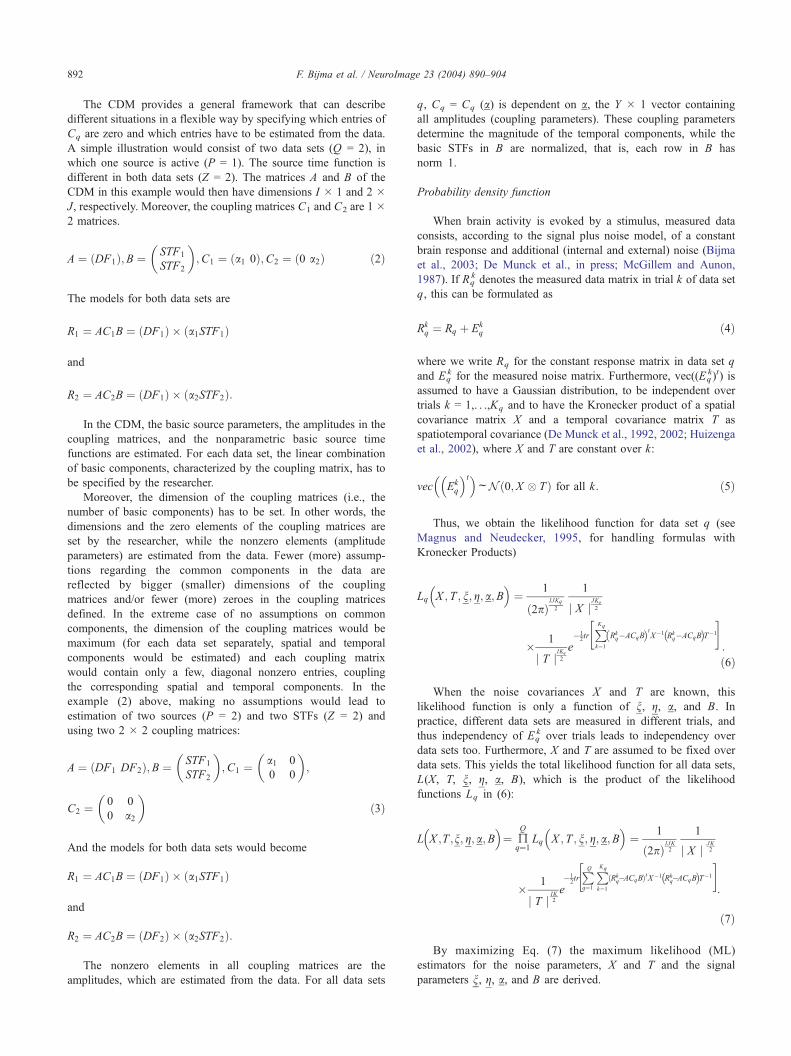
Table 1
Locations of simulated sources in simulation 1
Position source left (cm) Orientation source left
x y z x y z
Somatosensory 1.63 3.80 3.18 �0.83 0.47 �0.29
Visual �6.37 1.80 �2.82 �0.44 0.22 0.87
Auditive 0.63 4.30 �0.82 0.00 0.00 1.00
The positions of the sources are relative to the center of the spherical
volume conductor. Positions and orientations of the sources were taken
symmetric, i.e. with opposite y coordinates. The direction of the x axis is
forward, the y axis to the left, and the z axis upwards.
F. Bijma et al. / NeuroImage 23 (2004) 890–904894
HH n; g;B; a� �¼ tr R � IQ � A
� CB
� tR � IQ � A
� CB
� i:
hð23Þ
Now the SVD of R, containing the stacked prewhitened data of
all data sets, is calculated
R ¼ UDV t withUaRIQ�JUtU ¼ IJVaRJ�J VV t ¼ V tV ¼ IJDaRJ�J D ¼ diag k1; k2; N ; kJð Þ
8<: ð24Þ
and Eq. (23) is rewritten
HH n; g;B; a� �¼ tr UD � IQ � A
� CBV
� tUD � IQ � A
� CBV
� i:
hð25Þ
The trace in Eq. (25) is split into terms corresponding to the first
J0 largest eigenvalues of R and the remaining J � J0 terms:
HH n; g;B; a� �
¼XIQl¼1
XJ0j¼1
UD � IQ � A�
CBV� 2
l;j
þXIQl¼1
XJj¼ J0þ1
UD � IQ � A�
CBV� 2
l; jð26Þ
The dimensionality of the estimation problem is reduced by
setting the J � J0 small eigenvalues of R to zero and choosing B
such that [(IQ � A) CBV]l, j = 0 for j N J0 for all l. Then the
second term in Eq. (26) will vanish and the remaining cost
function is
HH n; g;B; a� �
¼XIQl¼1
XJ0j¼1
�UD � IQ � A
� CBV
�2
l;j
: ð27Þ
If the J � J truncated diagonal matrix is denoted by
D0 ¼ diag k1; k2; N ; kJ0 ; 0; N ; 0ð Þ ð28Þ
the estimators in Eqs. (14) and (17) to (20) change accordingly
into
BBML ¼�Ct IQ � AtA�
C��1
Ct IQ � At�
UD0Vt ð29Þ
Up1 ; p2 ¼ tr BtCt IQ � BAt
Bgp2
!IQ � BA
Bgp1
!CB
#"ð30Þ
/p ¼ tr V tBtCt IQ � BAt
Bgp
!UD0
#"ð31Þ
Wy1; y2 ¼ tr Bt BCt
Bay2IQ � At�
IQ � A� BC
Bay1B
��ð32Þ
wy ¼ tr V tBt BCt
BayIQ � At�
UD0
�:
�ð33Þ
Summarizing, the estimation procedure looks like
(1) Compute Rq for all q and X and T using Eqs. (9) and (10).
(2) Perform a global search over source locations to
obtain a starting point for the nonlinear (Marquardt)
algorithm.
(3) Iterate until convergence of the cost function H (n, g, B, a):(a) obtain an update for the positions in n in the Marquardt
algorithm (the first time, the starting point from the
global search is taken)
(b) iterate until convergence of H(n, g, B, a) for fixed n:(i) update B using Eq. (29),
(ii) iterate until convergence of H (n, g, B, a) for fixedn and B:
(A) update a using Eqs. (16), (32), and (33),
(B) update g using Eqs. (15), (30), and (31).
In the global search in step (2), a regular grid with locations is
computed. For each location, step (3b) is executed and the
converging value of the cost function H for that location is
computed. The location with the minimum value of the cost
function is taken as starting point in step (3). In step (2), alternative
initialization procedures can be used, as outlined in Uutela et al.
(1998).
Results
The coupled dipole model was applied in two simulation
studies and to one experimental data set. In the first simulation
study, a symmetric dipole pair was simulated representing three
different functional areas: the somatosensory cortex, the auditory
cortex, and the visual cortex. In the second simulation study, data
from two dipoles in the visual cortex of the same hemisphere were
generated in different ratios of activity. The experimental data
consisted of visual evoked field (VEF) MEG data. The visual
stimulus in this experiment consisted of a checkerboard pattern,
presented either in one hemifield or full-field to the subject.

Fig. 2. The two basic input STFs for simulation 1 multiplied by 1000,
which is the amplitude in all data sets.
F. Bijma et al. / NeuroImage 23 (2004) 890–904 895
Simulation study 1
In the first simulation study, activity from two single dipole
sources was generated. Three surrogate data sets were
produced: in the first data, the left source was simulated, in
the second, the right source and the third data set contained
simulated data from both sources. The locations of the sources
were taken symmetric and varied over the visual, auditory, and
somatosensory cortices. True locations of these cortices were
based on experimentally located positions (see Table 1). Two
basic source time functions were used to generate the data, see
Eqs. (36) and (37). For each location, 100 sweeps were generated.
The sample rate used was 625 Hz, and a time window of 32 ms
was analyzed. All data sets consisted of simulated dipole activity
and additional white noise with varying signal to noise ratio, SNR
equal to 1/3, 1, 3, and 9. The SNR is defined as the ratio between
the matrix powers of the surrogate signal and the surrogate white
noise:
SNR ¼tr Rt
sur R sur
� tr E t
sur E sur
� ð34Þ
The first data set contained activity from the left source with
STF1, the second activity from the right source with STF1, and the
third data set contained activity from both sources, both having STF2.
The matrix A(g, n) contained the forward fields of both dipoles,and B contained the two normalized basic STFs. The coupling
matrices for the three data sets were
C1 ¼a1 0
0 0
�;C2 ¼
0 0
a2 0
�;C3 ¼
0 a30 a4
����ð35Þ
Both input STFs were 10 Hz sinusoids:
STF1 tð Þ ¼ 1
n1sin 20ptð Þ ð36Þ
STF2 tð Þ ¼ 1
n2sin 20pt � p
4
� �þ 0:35
��ð37Þ
where n1 and n2 are the normalization constants, n1 ¼ffiffiffiffiffiffiffiffiffiffiffiffiffiffiffiffi11:5003
p
and n2 ¼ffiffiffiffiffiffiffiffiffiffiffiffiffiffiffiffi10:1852
p. The following coupling parameter values
were used
a1 ¼ 1000n1 ð38Þ
a2 ¼ 1000n1 ð39Þ
a3 ¼ 1000n2 ð40Þ
a4 ¼ 1000n2 ð41Þ
The absolute values of the magnitudes do not influence the
performance of the different localization methods. Only the
relative amount of noise, indicated by the SNR, counts. There-
fore, the a values were chosen such that the absolute magnitudes
were comfortable in the analysis. In Fig. 2, the input STFs are
plotted as function of time. Four different source localization
analyses were performed: the three data sets in three separate
analyses as presented in De Munck et al. (2002) and all data sets
simultaneously in the CDM. In the separate analyses, the
estimation of the source parameters was performed based on
the simulated number of sources: one source was localized in
data sets 1 and 2, and two sources were estimated in data set 3.
The grid for the global search consisted of 100 locations,
resulting in 100 possible starting points for data sets 1 and 2
and 100 � 99/2 = 4950 possible starting combinations for data
set 3. In the CDM analysis, two sources, two STFs, and nonzero
elements of the coupling matrices in Eq. (35) were estimated. The
same grid was used for the global search, yielding 100 � 99 =
9900 possible starting combinations of the two sources, because
the order of the sources is important in the CDM. Average errors in
position and orientation of the estimated dipoles as well as in
magnitude of the estimated source time functions were computed
for all four analyses. The averages were taken over the sweeps and
over both sources (position and orientation) or both STFs
(magnitude).
For all three cortex locations, the errors show a similar pattern:
the integrated analysis yields a lower error than the separate
analyses. Depending the distance between the sources, this differ-
ence in performance varies. The errors in position, orientation, and
magnitude show a similar pattern; therefore, only the position error
is shown in Fig. 3. In Fig. 3a, the average position error for the
simulated dipoles in the somatosensory cortex is shown; in Fig. 3b,
the auditory cortex; and in Fig. 3c, the visual cortex. Clearly, the
difference in performance between the separate approach and the
CDM is largest for two active dipoles in the visual cortex (Fig. 3c).
The reason for this is that the (lateral) distance between the simulated
visual dipoles is smallest. Therefore, localizing the two sources in
the classical way will be hampered by the reasons mentioned in the
introduction. For all analyses, Fig. 3 shows an improvement
(slightly) in position error for the integrated model, indicating that
adding more data into the parameter estimation is advantageous.
Simulation study 2
In the second simulation study, two sources in the visual
cortex, one in the striate and one in the extrastriate cortex, were
simulated in five different ratios of activity. Positions and
orientations were taken from experimentally located sources,
resulting in the sources being 3 cm apart from each other (Table
2). As in simulation 1, data consisted of simulated dipole
activity and white noise with varying SNR, SNR = 1/3, 1, 3,
and 9. Each data set contained 100 sweeps, the sample
frequency was 625 Hz, and a time window of 32 ms was
analyzed. The input source time functions were two sinusoids,

Fig. 3. Average position errors in simulation 1. The errors are given in cm on a logarithmic scale. The dashed lines correspond to the separate analyses and the
solid line indicates results of the CDM. Right corresponds to the data set with only the right source active, left to the data set with the left dipole active, and
BiLat to the data set with both sources active. (a) Position errors of the localized sources in the somatosensory cortex. (b) Position errors of the localized
sources in the auditory cortex. (c) Position errors of the localized sources in the visual cortex.
Table 2
Locations of simulated sources in simulation 2
Position (cm) Orientation
x y z x y z
Striate �6.37 1.30 �1.82 �0.15 0.59 0.79
Extrastriate �5.37 3.30 �3.82 0.70 0.60 �0.40
The positions of the sources are relative to the center of the spherical
volume conductor. The direction of the x axis is forward, the y axis to the
left, and the z axis upwards.
F. Bijma et al. / NeuroImage 23 (2004) 890–904896
15 Hz for the striate source and 20 Hz for the extrastriate
source
STF1 tð Þ ¼ 1
n3sin 30ptð Þ ð42Þ
STF2 tð Þ ¼ 1
n4sin 40ptð Þ: ð43Þ
where n3 ¼ffiffiffiffiffiffiffiffiffiffiffiffiffiffiffiffi10:4013
pand n4 ¼
ffiffiffiffiffiffiffiffiffiffiffiffiffiffiffiffi8:49828
pare the normalization
constants. The five data sets were generated using the coupling
matrices
C1 ¼1000n3 0
0 0
� �;C2 ¼
750n3 0
0 250n4
� �;
C3 ¼500n3 0
0 500n4
� �;C4 ¼
250n3 0
0 750n4
� �;
C5 ¼0 0
0 1000n4
� �;
ð44Þ
Fig. 4 shows the two input STFs. Six source localization analyses
were performed: the five data sets separately (DeMunck et al., 2002)
and all five data sets in the integrated model.
Furthermore, in the CDM analysis, diagonal coupling matrices
with two unknowns were used for all data sets. In other words, in the
CDM analysis, no advantage was taken of the knowledge that data
sets 1 and 5 contain activity of only one dipole, while this
information was exploited in the separate analyses.
For the global search, the same grid as in the first simulation
study was used. This resulted in 100 possible starting locations for
the separate analyses of data sets 1 and 5, 4950 possible
combinations for data sets 2, 3, and 4, and 9900 possible
combinations for the CDM (as the order of the sources is of
importance in the simultaneous model).
Outliers in the estimated sources were discarded. The outlier
criteria used are
position error N 7 cm ð45Þdistance between sources b 0:5 cm ð46Þmagnitude error ðrelative powerÞ N 10 ð47Þ
The first criterium designates localized sources in implausible
positions, which would be discarded in experimental analysis. The

Fig. 5. The average position error of the localized sources in the simulation
2. Striate1 corresponds to data set 1, Striate3/4 to data set 2, Striate1/2 to
data set 3, Striate1/4 to data set 4, and ExtraStriate to data set 5. The errors
are given in centimeters on a logarithmic scale. The dashed lines
correspond to the separate analyses and the solid line indicates results of
the CDM.
Fig. 4. The two basic input STFs for simulation 2 multiplied by 1000, the
maximum amplitude (data sets 1 and 5).
F. Bijma et al. / NeuroImage 23 (2004) 890–904 897
latter two criteria often concur and indicate two coinciding sources,
usually having opposite orientations and unreasonably high
magnitudes, as discussed in Introduction. In Table 3, the numbers
of outliers in the different localizations are given: only the three
data sets containing two active sources yielded outliers in the
separate analyses. The simultaneous CDM did not yield any
outliers.
Average position errors, orientation errors, and magnitude errors
were computed for all six analyses. The averages were computed
over the 100 sweeps (minus the outlying sweeps) and over both
sources and both STFs.
As in the first simulation, the graphs of the three types of error
resemble each other. Fig. 5 demonstrates the position errors for all
analyses. The errors in the separate analyses can be divided into
two groups; data set 1 and 5, which contain only one active source,
show a lower error than the remaining three data sets. This reflects
the common feature that one source is easier localized than two
sources. Nevertheless, the CDM yields the lowest position error.
Compared to the separate analyses, using the CDM, the position
error drops approximately by a factor of 10 for data sets 2, 3, and 4.
For data sets 1 and 5, there is still an improvement of roughly a
factor of 1.5 in the position error.
Experimental data
The CDM was applied to experimental MEG data of a visual
evoked field experiment. The visual stimuli consisted of checker-
board pattern onsets, presented either in the left or the right hemifield
or full-field, thus yielding three data sets per subject. The separate
analyses of this kind of conditions show nearby localized sources
with similar orientations for the different conditions, indicating that
the assumption of common sources is plausible. Moreover, the
estimated orientations are opposite (Di Russo et al., 2002; Kenemans
Table 3
The number of outliers in the six source localizations in simulation 2
SNR 1/3 1 3 9
Data set 1 0 0 0 0
Data set 2 6 1 1 1
Data set 3 0 2 1 4
Data set 4 16 16 19 18
Data set 5 0 0 0 0
CDM 0 0 0 0
et al., 2000); therefore, the solutions to the separate IPs are
susceptible for the canceling dipole problem. For this reason, the
behavior of the separate analyses and the CDM is compared using
these visual data.
Data of five subjects were considered in this study. The time
window of analysis was set to 80–112 ms post stimulus. The
sample rate was 625 Hz, the number of trials was 400 in each data
set. Similar to simulation 1, the three data sets were analyzed
separately, yielding three sets of estimated parameters, and the
CDM was applied to all three data sets simultaneously, yielding
one solution with estimated common spatial and common temporal
parameters.
The check size was 6V. Checks of this size mainly activate the
striate cortex in the chosen time interval (Di Russo et al., 2002;
Ossenblok et al., 1994). As expected, hemifield stimuli first
activate the contralateral hemisphere, with a peak at around 90–95
ms. However, between 10 and 15 ms (Saron and Davidson, 1989)
or 20 ms later (Steger et al., 2001), the ipsilateral hemisphere is
activated as well by inter-hemispheric transfer. In sum, to describe
the hemifield data, two sources are needed, having in the CDM two
different STFs: a contralateral STF and an ipsilateral STF. The
contralateral STF was also used to describe the time courses of
both sources in the bilateral data set, because these stimuli will
activate both hemispheres directly (Kenemans et al., 2000),
although maybe even faster (Steger et al., 2001). This yielded
the following basic and coupling matrices:
A ¼ DFleft DFright�
;B ¼ STFcontraSTFipsi
� �ð48Þ
Clh ¼0 a2a1 0
�;Crh ¼
a3 0
0 a4
�;Cff ¼
a5 0
a6 0
�;
���ð49Þ
where blhQ corresponds to the left hemifield stimulation, brhQ to the
right hemifield stimulation, and bffQ to the full-field stimulation.

Table 4
Estimated locations for subject 5 in the experimental study
Position source left (cm) Orientation source left Orientation source right
x y z x y z x y z
Data set LH 23 �5.21 1.29 0.94 0.26 0.96 0.11 0.26 �0.96 0.11
Data set LH 102 �5.21 1.29 0.94 0.26 0.96 0.11 0.26 �0.96 0.11
Data set RH 23 �6.14 1.21 0.17 0.17 0.76 0.62 0.00 0.12 0.99
Data set RH 102 �5.72 0.32 0.11 0.06 0.88 0.47 0.05 �0.96 �0.27
Data set FF 23 �4.42 0.00 �1.15 0.25 �0.05 �0.97 �0.25 0.05 0.97
Data set FF 102 �5.14 1.43 0.89 0.31 0.77 0.56 0.28 �0.96 0.08
CDM �5.25 1.44 0.85 0.30 0.72 0.62 0.28 �0.95 0.12
The positions of the localized sources are relative to the center of the spherical volume conductor. The positions of the two sources are symmetric. The direction
of the x axis is forward, the y axis to the left, and the z axis upwards.
F. Bijma et al. / NeuroImage 23 (2004) 890–904898
In all the analyses, a semisymmetric source pair was fitted.
Semisymmetric sources have symmetric locations (as in Di Russo
et al., 2002; Kenemans et al., 2000), but their orientations are
free. Nevertheless, the estimated orientations are nearly symmet-
ric (Table 4).
The number of locations in the regular grid for the global search
for the starting location of the semisymmetric dipole source was
varied over 23, 102, and 466 points in one hemisphere, correspond-
ing to mesh sizes of 4.2, 2.6, 1.5 cm, respectively.
The solutions to the separate IPs changed when the number
was increased from 23 to 102 grid points, but remained the same
for the increase from 102 to 466 points. The simultaneous model,
though, yielded the same solutions for all three grids. This shows
Fig. 6. Estimated STFs of the semisymmetric sources resulting from the separate a
(subject 5). The time indicated is the post stimulus time in milliseconds. The unit
stimulation data set. (b) The estimated STFs for the right hemifield stimulation d
that the CDM is less sensitive to local minima in the cost
function.
The results of the separate analyses varied considerably over
subjects. For subjects 1 and 2, the separate analyses yielded
plausible solutions for all three conditions for both 23 and 102 grid
points.
For subject 3, all three separate solutions to the IP consisted of a
pair of canceling, coinciding sources (intermediate distance b 0.01
cm). Even using a global search with 466 grid points yielded these
implausible solutions for all three separate models. Subject 4
yielded for the right hemifield data set a physiologically plausible
solution for all grids. For the coarse grid, the sources in the full-
field data set were localized in the cerebellum. For 102 grid
nalyses using a global search with 23 grid points in the experimental study
on the vertical axis is nAcm. (a) The estimated STFs for the left hemifield
ata set. (c) The estimated STFs for the full-field stimulation data set.

F. Bijma et al. / NeuroImage 23 (2004) 890–904 899
points, this problem was resolved and the solutions were
localized in the visual cortex. The locations of the sources in
the left hemifield data set showed a plausible location, though the
ipsilateral orientation differs from the usual lateral direction for
all grids. The corresponding amplitude is very small; therefore,
the total influence of this orientation on the cost function is very
small.
Subject 5 (see Table 4) yielded a solution consisting of a
canceling dipole pair for the full-field data set when the coarse grid
was used. For the denser grids, this data set yielded an interpretable
solution. The right hemifield data set yielded a location in the visual
cortex for 23 grid points, though the ipsilateral orientation was
unusual. For 102 and 466 grid points, these sources were localized
nearer to the midsagittal plane (1.2 cm in between). For all grids, left
hemifield data set yielded plausible solutions.
The simultaneous model yielded for all five subjects plausible
solutions for all conditions for all grids.
Summarizing, for the coarse grid, 5 of the 15 separate analyses
resulted in an implausible solution, and for the denser grids, 3 of the
15 conditions yielded a non-interpretable solution, whereas the
simultaneous model only yielded plausible solutions.
The results of subject 5 are representative for the type of errors
that can occur in the separate solutions; therefore, the analyses of this
subject for the coarse (23 points) and the dense (102 points) grid and
the CDM solution are presented. The estimated locations and
orientations of the sources for the seven different localizations are
reported in Table 4. The estimated STFs are shown in Figs. 6–8. Fig.
Fig. 7. Estimated STFs of the semisymmetric sources resulting from the separate a
(subject 5). The time indicated is the post stimulus time in milliseconds. The unit
stimulation data set. (b) The estimated STFs for the right hemifield stimulation d
6 shows the STFs estimated in the separate analyses using the coarse
grid, Fig. 7 the estimated STFs for the dense grid, and Fig. 8 displays
the estimated STFs for the simultaneous model that did not change
with the number of grid points.
In Fig. 6c, an example of the canceling dipole problem is shown:
the magnitudes are unrealistically high, the corresponding locations
in Table 4 coincide, and the estimated orientations are opposite. For
the coarse grid, the RH data set does not yield the usual lateral
orientation for the ipsilateral source. This orientation does not have a
substantial influence on the cost function, because the corresponding
amplitude (Fig. 6b) is rather small. The amplitudes in the different
analyses for the RH data set vary. In Fig. 7b (dense grid), the
estimated amplitudes are larger than the amplitudes shown in Figs.
6b (coarse grid) and 8b (CDM). The corresponding distance to the
midsagittal plane for the dense grid (0.32 cm) is smaller than for the
coarse grid and the CDM (1.21 and 1.44 cm, respectively). This may
indicate a slight cancellation of dipole activity: the sources are closer
and the amplitudes are higher for the dense grid.
Discussion
The coupled dipole model provides a method to solve the inverse
problem by analyzing multiple MEG data sets simultaneously when
these data sets contain common sources or common source time
functions. This way, more data are used and more constraints
(assumptions) are made to solve and stabilize the IP.
nalyses using a global search with 102 grid points in the experimental study
on the vertical axis is nAcm. (a) The estimated STFs for the left hemifield
ata set. (c) The estimated STFs for the full-field stimulation data set.

Fig. 8. Estimated STFs of the semisymmetric sources resulting from CDM analysis in the experimental study (subject 5). The time indicated is the post stimulus
time in milliseconds. The unit on the vertical axis is nAcm. (a) The estimated STFs for the left hemifield stimulation data set. (b) The estimated STFs for the
right hemifield stimulation data set. (c) The estimated STFs for the full-field stimulation data set.
F. Bijma et al. / NeuroImage 23 (2004) 890–904900
The results of the first simulation show that the position error
decreases when the integrated model is used instead of the separate
models. The gain in accuracy depends on the locations (intermediate
distance) of the sources to be localized and was largest for the
simulated sources in the visual cortex.
Simulation 2 displays a considerable improvement in source
localization for the CDM, studying two active dipoles in the visual
cortex in five different ratios of activity. For one of the five data sets
considered, a quarter striate and three quarters extrastriate activity,
the position error drops by a factor of 10 when the CDM is used
instead of a single model. Moreover, outliers only occurred in the
separate analyses of data sets 2, 3, and 4, while the CDM did not
yield any outliers (see Table 3). In Fig. 5, it can be seen that the
position error of data set 4 is higher for SNR = 3 than it is for SNR =
1. A similar feature was found in the orientation andmagnitude error.
This contradicts the fact that for higher SNR the error decreases. The
reason for this slight increase in error lies in the outlier problem. For
all SNR values in data set 4, some sweeps were marked as outlier
(45) and discarded. However, some other sweeps, not indicated as
outlier, also showed a rather large position error (N2 cm), but
within the outlier criterium of 7 cm. For SNR = 1, the number of
these semi-outlying sweeps was lower than for SNR = 1/3 and
SNR = 3. Because these sweeps raise the average error remarkably,
this difference between SNR = 1 and the other SNR values
explains the error shape in Fig. 5. Increasing the number of sweeps
considerably or redefining the outlier criteria should eliminate this
problem. This shows that the choice of outlier criteria is delicate.
Nonetheless, this outlier problem is not present in the CDM (Table
3), which is an important advantage of the integrated approach
regarding the stability of the solution.
The application of the CDM to experimental VEF data showed
that in 5 (coarse grid) or 3 (dense grid) of the 15 conditions
considered, no interpretable solution was obtained without using the
CDM. The classic (separate) analysis of all but one of these
conditions yielded a canceling dipole source pair, and one condition
yielded a localized visual source pair in the cerebellum (coarse grid).
The CDM yielded invariably plausible solutions. This demonstrates
that the CDM is not sensitive for minima in the cost function that
correspond to a canceling dipole pair. The underlying reason may be
that these minima of the separate cost functions occur at different
locations for different conditions and will therefore not produce a
minimum in the simultaneous cost function.
Another advantage of the simultaneous model is the direct
comparability of the estimated magnitudes. Because all parameters
are estimated in one analysis, the magnitudes between conditions
can directly be compared (Fig. 8), while the separate analyses (Figs.
6 and 7) use for different conditions different scalings and it is
difficult to compare the absolute magnitudes between conditions.
This difference in scaling is caused by the depth bias (the mutual
dependence of depth and amplitude) and possible slight cancellation
of the sources (cf. RH for the coarse grid) and the differences in STF
shapes between conditions.
Summarizing, the experimental application showed that simul-
taneously estimating the amplitudes and locations in the three data
sets yields more stable and comparable estimated parameters, while
separate models are more vulnerable for implausible minima and
yield in general estimated magnitudes and positions that vary over
data sets.
The estimation procedure for the signal parameters presented in
this paper is computationally intensive due to the nested iterations in

F. Bijma et al. / NeuroImage 23 (2004) 890–904 901
the estimation procedure. It is our intention to improve the method to
overcome this drawback.
Designing the coupling matrices is subject to the choice (or a
priori knowledge) of the user. Different users may want to design the
coupling matrices in a different way. This is both a flexibility
property of the model and a subjectivity of the CDM. The user can
make more or less assumptions by adapting the dimension of the
coupling matrices, as was shown in the example in Eqs. (2) and (3).
Such assumptions, in fact, are also made when similar data sets are
analyzed using separate analyses: results are compared afterwards
and conclusions are drawn about the similarity of sources and
source time functions in the different data sets. The CDM now
provides a way to put this knowledge a priori in the source
localization method, which relatively increases the SNR. If the user
is not sure about certain similarities, the coupling matrices should
be extended to less assumptions. In the second simulation study,
the robustness of the CDM was tested by applying less
assumptions than possible (fitting two sources when only one
was active in data sets 1 and 5), and it was shown that the CDM
still estimates the sources and STFs well.
A possible extension of the CDM would be the simultaneous
analysis of data sets of different subjects and/or different conditions.
If it is assumed that the spatial and temporal covariances differ only
slightly over subjects and conditions (Bijma et al., 2003; De Munck
et al., 2002), and can therefore be fixated, this extension is rather
straightforward. This kind of extension will be helpful if one is
interested in grand averages of, for example, amplitude functions or
source positions as in cognitive neuroscience (Di Russo et al., 2002;
Kenemans et al., 2000).
In all, the CDM combines multiple data sets and extra constraints
into one integrated model to solve and stabilize the ill-posed inverse
problem in MEG/EEG, yielding interpretable solutions, in cases
where separate models not always yield plausible solutions.
Appendix A. Dimensions and variables
The dimensions are defined as
IZ # sensors ð50Þ
JZ # time samples ð51Þ
KqZ # trials in data set q ð52Þ
KZ # trials in all data sets ð53Þ
PZ # basic sources ð54Þ
QZ # data sets ð55Þ
YZ # amplitude parameters ð56Þ
ZZ # basic STFs ð57Þ
and the variables as
aZY � 1 vector containing amplitude parameters ð58Þ
gZ3P � 1 vector with sources orientations ð59Þ
nZ3P � 1 vector with source locations ð60Þ
A n; g� �
ZI � P forward field matrix of basic dipoles ð61Þ
AZIQ� IP matrix : IQ � A ð62Þ
BZZ � J basic STF matrix; with basic STFs as rows ð63Þ
BZZ � J prewhitened STF matrix ð64Þ
CqZP � Z coupling matrix for data set q ð65Þ
CZPQ� Z stacked coupling matrices ð66Þ
E kqZI � J noise matrix of trial k in data set q ð67Þ
InZn� n identity matrix ð68Þ
R kqZI � J data matrix of trial k in data set q ð69Þ
RqZI � J model matrix for data set q ð70Þ
RRqZI � J average data matrix for data set q ð71Þ
Appendix B. ML estimators for X and T
This derivation uses the following two matrix derivatives
(Magnus and Neudecker, 1995, chapter 9)
dX jX jð Þ ¼ jX jtr X�1dX�
and
dX X�1�
¼ � X�1dXX�1:
The derivative of L(X, T, n, g, a, B) in Eq. (7) with respect to X is
dX L ¼ L�"
� JK2djX j
jX j þ dX � 1
2trXQq¼1
XKq
k¼1
Rkq � RRqB
� �tX�1
"
� Rkq � RRq
� �T�1
#!#
¼ 1
2L�
"� JKjX jtr X�1dXð Þ
jX j
þ trXQq¼1
XKq
k¼1
Rkq � RRq
� �tX�1dXX�1 Rk
q � RRq
� �T�1
#" #
¼ 1
2L� tr � JK þ
XQq¼1
XKq
k¼1
X�1 Rkq � RRq
� �T�1
" "
� Rkq � RRq
� �t#X�1dX
!#ð72Þ
F. Bijma et al. / NeuroImage 23 (2004) 890–904902
The optimal spatial covariance matrix, XML, is obtained when
dXL = 0, that is, when"� JK þ
XQq¼1
XKq
k¼1
XX �1ML Rk
q � RRq
� �T�1 Rk
q � RRq
� �t#XX �1
ML
¼ 0 , XX ML ¼ 1
JK
XQq¼1
XKq
k¼1
Rkq � RRq
� �T�1 Rk
q � RRq
� �t; ð73Þ
provided that XML is nonsingular. Similarly for T, the estimator
becomes
TT ML ¼ 1
IK
XQq¼1
XKq
k¼1
Rkq � RRq
� �tX�1 Rk
q � RRq
� �: ð74Þ
Appendix C. ML estimator for B
Although the rows in B are normalized, the ML estimator for B
is derived as if B were unconstrained. The rows are normalized
afterwards.
dBL ¼ 1
2L� tr
XQq¼1
XKq
k¼1
ACqdB� t
X�1 Rkq � ACqB
� �T�1
"
þ Rkq � ACqB
� �tX�1ACqdBT
�1
#
¼ L� trXQq¼1
XKq
k¼1
T�1 Rkq � ACqB
� �tX�1ACqdB
#:
"ð75Þ
Setting this derivative to zero yields the estimator for B:
XQq¼1
XKq
k¼1
T�1 Rkq � ACqBBML
� �tX�1ACq ¼ 0
,XQq¼1
XKq
k¼1
Rkq
� �tX�1ACq
¼XQq¼1
XKq
k¼1
ACqBBML
� tX�1ACq
, BBML ¼XQq¼1
KqCtqA
tX�1ACq
!�1XQq¼1
XKq
k¼1
CtqA
tX�1 Rkq
� �t;
ð76Þ
provided thatPQ
q¼1 KqCtqA
tX�1ACq is invertible. After this
estimator has been calculated, the STFs in B are normalized.
Appendix D. ML estimator for orientation parameters h in A
The source parameters in A can be split into the linear
orientation parameters g, and the nonlinear position parameters n.If all P sources are modeled as single dipoles or symmetric
source pairs, g and n will both be 3P � 1 vectors. If P
semisymmetric source pairs (symmetric location, free orientation)
are used, g will be 6P � 1 and n will be 3P � 1. For notational
clarity, g and n will both be assumed to be 3P � 1. For the case
of semisymmetric sources, the dimensions have to be adjusted
correspondingly. The linear parameters g are estimated in the
usual ML sense; setting the derivative of L equal to zero. The
nonlinear parameters n are determined using the Marquardt
algorithm. The derivative of L with respect to g is calculated by
first computing dAL and subsequently applying the chain rule.
dAL ¼ 1
2L� tr
XQq¼1
XKq
k¼1
dACqB� t
X�1 Rkq � ACqB
� �T�1
"
þ Rkq � ACqB
� �tX�1dACqBT
�1
#
¼ L� trXQq¼1
XKq
k¼1
CqBT�1 Rk
q � ACqB� �t
X�1dA
#:
"ð77Þ
Writing g = (g1, . . ., g3P) and applying the chain rule for the
source parameter gp yields
dgpL ¼ L� trXQq¼1
XKq
k¼1
CqBT�1 Rk
q � ACqB� �t
X�1 BA
Bgp
#dgp
"ð78Þ
To obtain the ML estimate for gp, this derivative is set to zero.
dgpL ¼ 0 , trXQq¼1
XKq
k¼1
CqBT�1 Rk
q � ACqB� �t
X�1 BA
Bgp
#¼ 0
"
, trXQq¼1
XKq
k¼1
CqB�1�Rkq
�tX�1 BA
Bgp
#"
¼ trXQq¼1
XKq
k¼1
CqBT�1BtCt
qAtX�1 BA
BDp
#"ð79Þ
Because the basic field matrix A is linear in g, it can be written as
A ¼X3Pp¼1
BA
Bgpgp ð80Þ
where BA/Bgp is independent of g. Eq. (79) holds for p = 1,. . .,3P
and substituting Eq. (80) into Eq. (79) yields
trXQq¼1
XKq
k¼1
CqBT�1 Rk
q
� �tX�1 BA
Bgp
#"
¼ tr
" XQq¼1
X3PpV¼1
KqCqBT�1BtCt
q
BAt
BgpVX�1 BA
Bgp
#gpV for all p
, Ug ¼ /
ð81Þ
where
Up1 ;p2 ¼ trXQq¼1
KqCqBT�1BtCt
q
BAt
Bgp2X�1 BA
Bgp1
#"ð82Þ

F. Bijma et al. / NeuroImage 23 (2004) 890–904 903
and
/p ¼ trXQq¼1
XKq
k¼1
CqBT�1 Rk
q
� �tX�1 BA
Bgp
#:
"ð83Þ
The linear parameters gp are solved from the linear system in
Eq. (81).
Appendix E. ML estimator for amplitude parameters in C
Analogous to the moment parameters, the amplitude parameters
a in the coupling matrices Cq are estimated using the chain rule.
Writing a = (a1, . . ., aY) the derivative with respect to ay is
day L ¼ 1
2L� tr
XQq¼1
XKq
k¼1
AdayCqB� t
X�1 Rkq � ACqB
� �T�1
"
þ Rkq � ACqB
� �tX�1AdayCqBT
�1
#
¼ L� trXQq¼1
XKq
k¼1
BT�1 Rkq � ACqB
�tX�1AdayCq
# "
¼ L� trXQq¼1
XKq
k¼1
BT�1 Rkq � ACqB
� �tX�1A
BCq
Bay
#day:
"ð84Þ
The ML estimators for ay satisfy
day L ¼ 0 , trXQq¼1
XKq
k¼1
BT�1 Rkq � ACqB
� �tX�1A
BCq
Bay
#¼ 0
"
, trXQq¼1
XKq
k¼1
BT�1 Rkq
� �tX�1A
BCq
Bay
#"
¼ trXQq¼1
XKq
k¼1
BT�1BtCtqA
tX�1ABCq
Bay
#:
"ð85Þ
Similar to the decomposition of A in Eq. (80), we can decompose
Cq due to the linearity in a:
Cq ¼XYy¼1
BCq
Bayay ð86Þ
for q = 1,. . . Q, with BCq/Bay independent of a. Eq. (85) holds fory = 1,. . .,Y. Formula (86) is substituted in formula (85), and we
obtain
trXQq¼1
XKq
k¼1
BT�1 Rkq
� �tX�1A
BCq
Bay
#"
¼ tr
" XQq¼1
XYyV¼1
KqBT�1Bt
BCtq
BayVAtX�1A
BCq
Bay
#ayVfor all y
, Wa ¼ w;
ð87Þ
where
Wy1;y2 ¼ trXQq¼1
KqBT�1Bt
BCtq
Bay2AtX�1A
BCq
Bay1
#"ð88Þ
and
wy ¼ trXQq¼1
XKq
k¼1
BT�1 Rkq
� �tX�1A
BCq
Bay
#:
"ð89Þ
This linear system solves the amplitude parameters a in Cq.
References
Achim, A., Bouchard, S., 1997. Toward a dynamic topographic
components model. Electroencephalogr. Clin. Neurophysiol. 103,
381–385.
Bijma, F., de Munck, J.C., Huizenga, H.M., Heethaar, R.M., 2003. A
mathematical approach to the temporal stationarity of background noise
in MEG/EEG measurements. NeuroImage 20 (1), 233–243.
de Munck, J.C., Vijn, P.C.M., Lopes da Silva, F.H., 1992. A random dipole
model for spontaneous brain activity. IEEE Trans. Biomed. Eng. 39 (8),
791–804.
de Munck, J.C., Huizenga, H.M., Waldorp, L.J., Heethaar, R.M., 2002.
Estimating stationary dipoles from MEG/EEG data contaminated with
spatially and temporally correlated background noise. IEEE Trans.
Signal Process. 50 (7), 1565–1572.
de Munck, J.C., Bijma, F., Gaura, P., Sieluzycki, C., Branco, M.I.,
Heethaar, R.M., in press. A mathematical description of habituaQ
tion effects in multichannel MEG/EEG data. IEEE Trans. Biomed.
Eng.
Di Russo, F., Martinez, A., Sereno, M.I., Pitzalis, S., Hillyard, S.A., 2002.
Cortical sources of the early components of the visual evoked potential.
Hum. Brain Mapp. 15 (2), 95–111.
Field, A.S., Graupe, D., 1991. Topographic component (parallel factor)
analysis of multichannel evoked potentials: practical issues in trilinear
spatiotemporal decomposition. Brain Topogr. 3, 407–423.
Huizenga, H.M., de Munck, J.C., Waldorp, L.J., Grasman, R.P.P.P.,
2002. Spatiotemporal EEG/MEG source analysis based on a para-
metric noise covariance model. IEEE Trans. Biomed. Eng. 49 (6),
533–539.
Kenemans, J.L., Baas, J.M.P., Mangun, G.R., Lijffijt, M., Verbaten,
M.N., 2000. On the processing of spatial frequencies as revealed
by evoked potential source modeling. Clin. Neuroph. 111 (6),
1113–1123.
Magnus, J.R., Neudecker, H., 1995. Matrix Differential Calculus with
Applications in Statistics and Econometrics, Revised Edition. John
Wiley and Sons, Chichester.
McGillem, C.D., Aunon, J.I., 1987. Analysis of event-related potentials. In:
Gevins, A.S., Remond, A. (Eds.), Methods of Analysis of Brain
Electrical and Magnetic Signals, EEG Handbook. Elsevier, Amsterdam,
pp. 131–169.
Mfcks, J., 1988. Topographic components models for event related
potentials and some biophysical considerations. IEEE Biomed. Eng.
35 (6), 482–484.
Ossenblok, P., Reits, D., Speckreijse, H., 1994. Check size dependency of
the sources of the hemifield-onset evoked-potential. Ophthalmologica
88 (1), 77–88.

F. Bijma et al. / NeuroImage 23 (2004) 890–904904
Saron, C.D., Davidson, R.J., 1989. Visual evoked potential measures of
interhemispheric transfer time in humans. Behav. Neurosci. 103 (5),
1115–1138.
Scherg, M., Von Cramon, D., 1985. Two bilateral sources of the late AEP as
identified by a spatio-temporal dipole model. Electroencephalogr. Clin.
Neurophysiol. 62, 32–44.
Steger, J., Imhof, K., Denoth, J., Pascual-Marqui, R.D., Steinhausen, H.C.,
Brandeis, D., 2001. Brain mapping of bilateral visual interactions in
children. Psychophysiology 38 (2), 243–253.
Turetsky, B., Raz, J., Fein, G., 1990. Representation of multi-channel
evoked potential data using a dipole component model of intracranial
generators: application to the auditory P300. Electroencephalogr. Clin.
Neurophysiol. 76, 540–556.
Uutela, K., H7m7l7inen, M., Salmelin, R., 1998. Global Optimization in the
Localization of Neuromagnetic Sources. IEEE Biomed. Eng. 45 (6),
716–723.
Wang, K.M., Begleiter, H., Porjesz, B., 2000. Trilinear modeling of event-
related potentials. Brain Topogr. 12 (4), 263–271.