The Coupled GCM ECHO-2. Part II: Indian Ocean Response to ENSO · Part II: Indian Ocean Response to ENSO ... better representation of the low-level stratus clouds, and ... area during

15 APRIL 2000 1371V E N Z K E E T A L .

q 2000 American Meteorological Society

The Coupled GCM ECHO-2. Part II: Indian Ocean Response to ENSO

STEPHAN VENZKE, MOJIB LATIF, AND ANDREAS VILLWOCK

Max-Planck-Institut fur Meteorologie, Hamburg, Germany

(Manuscript received 29 October 1997, in final form 17 June 1999)

ABSTRACT

The interannual variability of the Indian Ocean SST is investigated by analyzing data from observations andan integration of a global coupled GCM (CGCM) ECHO-2. First, it is demonstrated that the CGCM is capableof producing realistic tropical climate variability. Second, it is shown that a considerable part of the interannualvariability in Indian Ocean SST can be described as the response to interannual fluctuations over the Pacificrelated to ENSO. Although the Indian Ocean region also exhibits ENSO-independent interannual variability,this paper focuses on the ENSO-induced component only. Large-scale SST anomalies of the same sign as thoseobserved in the eastern equatorial Pacific Ocean during ENSO extremes develop in the entire tropical andsubtropical Indian Ocean with a time lag of about 4 months. This lead–lag relationship is found in both theobservations and the CGCM. Using the CGCM output, it is shown that the ENSO signal is carried into theIndian Ocean mainly through anomalous surface heat fluxes.

1. Introduction

In the first part of this series, Frey et al. (1997) de-scribed the mean state, annual cycle, and interannualvariability over the tropical Pacific as simulated by thesecond cycle of our coupled ocean–atmosphere generalcirculation model (CGCM), hereinafter referred to asECHO-2. Several aspects of the improved model’s per-formance over the Pacific Ocean with respect to the firstversion of the model, hereinafter referred to as ECHO-1,were discussed in Frey et al. (1997). The mean state,the annual cycle, and the interannual and decadal var-iability as simulated by ECHO-1 were investigated inseveral studies (Latif et al. 1994; Schneider et al. 1996;Latif and Barnett 1994, 1996; Grotzner et al. 1998).Modifications in the atmospheric convection scheme, abetter representation of the low-level stratus clouds, anda new numerical scheme for active tracer advection inthe ocean model improved the coupled model behavior.The latter results in a better simulation of the thermo-cline, causing the sea surface temperature (SST) to bemore sensitive to thermocline perturbations and there-fore leading to enhanced interannual variability in thecoupled integration with ECHO-2.

Large-scale air–sea interactions play a crucial role ingenerating interannual variability in the Tropics. Theclassical example for such air–sea interactions is the ElNino–Southern Oscillation (ENSO) phenomenon,

Corresponding author address: Dr. Mojib Latif, Max-Planck-In-stitut fur Meteorologie, Bundesstr. 55, 20146 Hamburg, Germany.E-mail: [email protected]

which is the strongest climate fluctuation on the short-range climatic timescale from a few months to severalyears [see the textbook of Philander (1990) for a goodoverview]. Because the ENSO signal is strongest in thetropical Pacific, much less attention has been paid sofar to the interannual variabilities of the tropical Indianand Atlantic Ocean and only a few papers exist thataddress these issues. Several studies have addressed theinteraction of interannual variability over the tropicalIndian Ocean with the Asian monsoon. Shukla (1987)as well as Ju and Slingo (1995) found that strongerwesterly winds associated with strong monsoon yearstend to cool down the ocean surface in the northwestIndian Ocean and the Arabian Sea in the postmonsoonmonths. On the other hand, several studies (e.g., Websterand Yang 1992; Ju and Slingo 1995; Soman and Slingo1997) suggest a clear relationship between the strengthof the large-scale monsoon circulation and the phase ofENSO: years with warm SST anomalies in the centraland east Pacific have a weaker monsoon circulation anda delayed onset. Opposite behavior is noted for thoseyears with cold SST anomalies in the eastern equatorialPacific Ocean. Latif and Barnett (1995) conclude froman investigation of several model integrations and ob-servations that air–sea interactions in the Indian andAtlantic Ocean are much weaker than those in the Pa-cific Ocean but that they, nevertheless, contribute to theinterannual variability in these regions, because theyamplify the ENSO-induced signal. In particular, the SSTanomalies in the tropical Pacific Ocean were found toforce SST anomalies of the same sign in the IndianOcean. In turn, there was no evidence that the Indian

1372 VOLUME 13J O U R N A L O F C L I M A T E

Ocean can significantly affect the ENSO cycle. In linewith these results are the findings of Kiladis and Diaz(1989), who describe an in-phase response of the trop-ical Indian Ocean SST to ENSO and suggest radiationalforcing and local wind stress changes as possible causes.

In this study, we examine the ENSO response of theIndian Ocean by analyzing observations and the outputof a 20-yr integration with our ECHO-2 CGCM. Thepaper is organized as follows: In section 2 a brief de-scription of the coupled model and the simulated tropicalmean state and the seasonality are given. The ENSO-related tropical variability is examined in section 3. Insection 4, we derive the physical processes causing theIndian Ocean response to ENSO. The paper is concludedwith a summary of our major findings in section 5.

2. Model description and tropical mean state

A detailed description of the CGCM ECHO-2 andespecially the changes made in respect to the earlierversion ECHO-1 was given in Part I of this series (Freyet al. 1997). Therefore, we restrict ourselves to a ratherbrief model description.

The coupled atmosphere–ocean model ECHO-2 is setup from cycle 4 of the Hamburg atmosphere GCM,(ECHAM; Roeckner et al. 1996) and the HamburgOcean Primitive Equation GCM, (HOPE; Wolff et al.1997).

ECHAM-4 is a global low-order spectral model witha triangular truncation at wavenumber 42 (T42). Thenonlinear terms and the parameterized physical pro-cesses are calculated on a 128 3 64 Gaussian grid,which yields a horizontal resolution of about 2.88 32.88. There are 19 levels in the vertical that are definedon sigma surfaces in the lower troposphere and on psurfaces in the upper troposphere and the stratosphere.

ECHAM-4 is coupled to the HOPE model withoutapplying flux correction. They interact over all threeoceans in the region 608N–608S. Since we have not yetincluded a sea-ice model, the SSTs are relaxed to Levitus(1982) climatology poleward of 608.

The ocean model is forced by the surface wind stress,the surface heat flux, and the freshwater flux simulatedby the atmospheric model. It uses a realistic bottomtopography. The model has a 2.88 resolution, with themeridional resolution gradually increased to 0.58 withinthe region 108N–108S. Vertically, there are 20 irregu-larly spaced levels, with 10 levels within the upper 300m. As described in Latif et al. (1994), solar radiation isallowed to penetrate beneath the first ocean layer. Thenumerical scheme of the ocean model uses the ArakawaE-grid (Arakawa and Lamb 1977) with a 2-h time step.

The simulated SST is used to force the ECHAM mod-el. The coupling is synchronous, with exchange of in-formation every 2 h. A 360-day year subdivided in 12equal-length months of 30 days is used. The coupledGCM is forced by seasonally varying insolation. Theoceanic initial conditions are taken from Levitus (1982)

climatology and those for the atmospheric model froma control run with climatological SSTs. The coupledintegration is started on 1 January and continued for 20yr. Pierce et al. (2000) carried the integration on foranother 120 yr. Their results confirm that the decadesanalyzed in this paper are representative of the model’sinterannual variability. To avoid effects of the initiali-zation we omit the first 2 yr of the integration in ouranalysis.

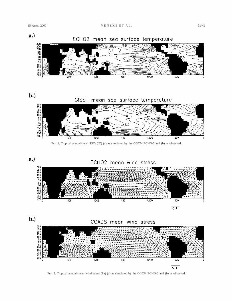
The SST is a key quantity by which the performanceof coupled models can be evaluated. In Fig. 1 we displaythe tropical annual-mean SSTs as simulated in our cou-pled model integration and the mean observed tropicalSSTs as derived from the SST dataset of the U.K. Me-teorological Office (UKMO), which is referred to as theGlobal Sea-Ice and Sea Surface Temperature (GISST)dataset, for the period 1949–91. At this point it shallbe mentioned that the simulated SST represents the tem-perature of the top model layer (i.e., upper 20 m). Thesimulation with ECHO-2 shows a cold bias in the equa-torial Pacific. However, the warm pool/cold tonguestructure is simulated with more success by the newversion of the model, since the numerical effective dif-fussion in the ocean model is reduced. In the IndianOcean the observed mean state of the SSTs is fairly wellreproduced by our coupled GCM.

As shown in Fig. 2, the annual-mean wind stress isalso realistically simulated in ECHO-2. Over the south-ern tropical Indian Ocean we find southeasterly tradewinds of equal strength and orientation as those derivedfor 1949–91 from the Comprehensive Ocean–Atmo-sphere Data Set (COADS; da Silva et al. 1994). Westerlywinds with similar strength are found north of the equa-tor in both the observations and our CGCM integration.Only the wind stresses over the Arabian Sea are notproperly simulated by ECHO-2. As can be seen in Fig.3, this deficiency has to be attributed to an overesti-mation of the northeasterly winds in winter, which seemsto be due to the simulation of too cold air temperaturesover Siberia by the ECHAM-4 model. Otherwise, themonsoon circulation over the Arabian Sea is simulatedquite well by the coupled GCM, both in terms of phaseand amplitude (Fig. 3c). As a result of too strong windsover the Arabian Sea in winter (December–February,hereafter DJF) the latent heat loss is enhanced in winter(DJF), which leads to colder than observed SSTs in thisarea during late winter and spring (Fig. 3d). Apart froma slightly delayed onset of the summer monsoon, how-ever, these SST errors appear not to affect the qualityof the simulated monsoon circulation. Furthermore, theassociated seasonal variations of the surface currents arewell simulated (Fig. 4). As in Murtugudde et al. (1996),the reversal of the Somali Current from February toAugust is clearly seen in the model results. Due to thecoarser zonal resultion, the speed of the Somali Currentis significantly lower than in Murtugudde et al. (1996).The seasonality of the South Equatorial Counter Cur-rent, which is fed by the southward Somali Current in


FIG. 1. Tropical annual-mean SSTs (8C) (a) as simulated by the CGCM ECHO-2 and (b) as observed.

FIG. 2. Tropical annual-mean wind stress (Pa) (a) as simulated by the CGCM ECHO-2 and (b) as observed.


FIG. 3. Climatological seasonal-mean surface wind stress (Pa) for boreal summer (Jun–Aug) and winter (Dec–Feb) (a) as simulated by theCGCM ECHO-2 and (b) as observed.

February, and of the South Equatorial Current are alsoin agreement with the results of Murtugudde et al.(1996). During the transition periods of the monsoon,the model produces a wind-driven eastward equatorialjet (Wyrtki 1973) that peaks around May and appearsagain in December. The latter maximum is late by morethan a month compared to the observations of Reverdin(1987), which is due to a phase error of the zonal windson the equator as discussed below. Furthermore, theseasonal reversal of the flow direction in the Bay ofBengal and south of Sri Lanka is well captured by theECHO-2 model.

Details about the annual-mean state and the annual

cycle in the tropical Pacific as well as a comparison ofthe integration of ECHO-2 with earlier integrations ofECHO-1 are given in Part I of this series (Frey et al.1997). In this part, we shall investigate the interannualvariablity in the ECHO-2 integration and focus on theIndian Ocean response to ENSO.

3. ENSO-related tropical variability

The most apparent improvement relative to the sim-ulation with the previous model version ECHO-1 is theenhanced level of interannual variability in ECHO-2.To emphasize the interannual fluctuations, the anomalies


FIG. 3. (Continued ) (c) Seasonality of the simulated and observed wind stress over the Arabian Sea (Pa) averaged over 108–208N and608–708E. (d) Same as (c) but for SST (8C).

FIG. 4. Simulated climatological mean surface currents (m s21) for Feb and Aug.

have been slightly smoothed using a 13-month runningmean filter. This, however, does not effect any of thequalitative results of this paper. The model simulates,for instance, interannual SST anomalies in the equatorialPacific (Figs. 5 and 6). In comparison with observations,the amplitude of these anomalies is roughly a factor oftwo too small (note the scale in Fig. 5) and the periodis slightly too short. However, the interannual variabilityis simulated more realistically than in the ECHO-1 mod-el. This is due to a better simulation of the thermocline,which has been achieved by changing the numericaltreatment of tracer advection. Considerably less effec-

tive mixing inhibits an erosion of the thermocline mak-ing the SST more sensitive to thermocline perturbationsin the eastern equatorial Pacific and therefore enhancingthe interannual variability in this region in the coupledrun with ECHO-2.

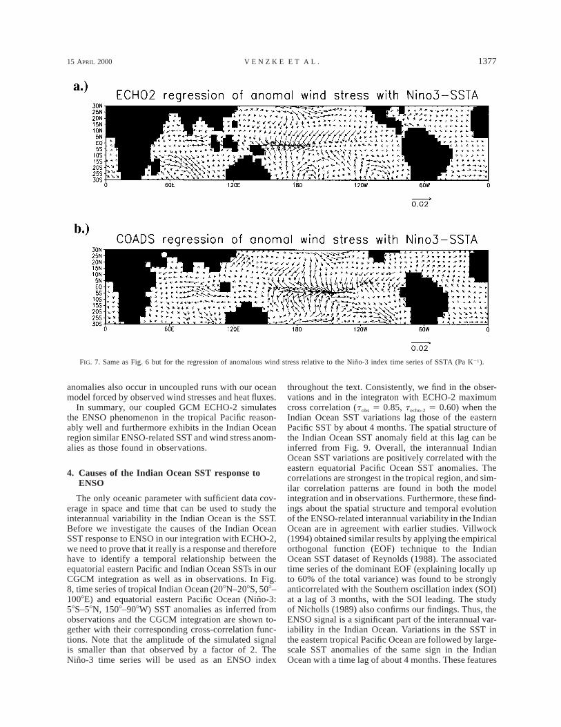
The spatial structures of the interannual SST anom-alies and the associated wind stress anomalies are shownin Figs. 6 and 7, respectively. Overall, the anomalystructures are simulated reasonably well, with SSTanomalies centered in the eastern equatorial Pacific, ac-companied by westerly wind stress anomalies in thewestern equatorial Pacific. In agreement with the ob-


FIG. 5. Time series of (a) model-simulated and (b) observed SST anomalies averaged over the Nino-3 index region (58S–58N, 1508–908W). The data were smoothed using a 13-month running mean filter.

FIG. 6. Spatial distribution of SSTA regression coefficients relative to the Nino-3 index time series as derived from (a) the integration ofthe CGCM ECHO-2 and (b) observations (1949–91). The data were smoothed using a 13-month running mean filter prior to the analysis.

servations, large-scale SST anomalies of the same signas those in the eastern equatorial Pacific and associatedwestward wind stress anomalies in the equatorial IndianOcean are simulated by ECHO-2. There are, however,some differences between the simulation and observa-tions. The simulated SST anomalies are too much equa-torially confined, and they extend too far into the west-

ern Pacific. The latter deficiency is related to the coldtongue, which is too strong and extends too far into thewestern Pacific. Furthermore, the coupled model un-derestimates the strength of the off-equatorial SSTanomalies of opposite sign in the Pacific. The reasonfor these errors seems to be inherent to the ocean model,since the problems in simulating the ENSO related SST


FIG. 7. Same as Fig. 6 but for the regression of anomalous wind stress relative to the Nino-3 index time series of SSTA (Pa K21).

anomalies also occur in uncoupled runs with our oceanmodel forced by observed wind stresses and heat fluxes.

In summary, our coupled GCM ECHO-2 simulatesthe ENSO phenomenon in the tropical Pacific reason-ably well and furthermore exhibits in the Indian Oceanregion similar ENSO-related SST and wind stress anom-alies as those found in observations.

4. Causes of the Indian Ocean SST response toENSO

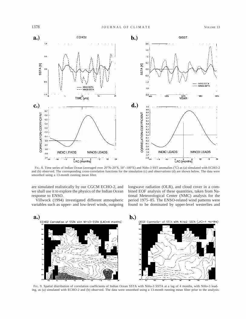
The only oceanic parameter with sufficient data cov-erage in space and time that can be used to study theinterannual variability in the Indian Ocean is the SST.Before we investigate the causes of the Indian OceanSST response to ENSO in our integration with ECHO-2,we need to prove that it really is a response and thereforehave to identify a temporal relationship between theequatorial eastern Pacific and Indian Ocean SSTs in ourCGCM integration as well as in observations. In Fig.8, time series of tropical Indian Ocean (208N–208S, 508–1008E) and equatorial eastern Pacific Ocean (Nino-3:58S–58N, 1508–908W) SST anomalies as inferred fromobservations and the CGCM integration are shown to-gether with their corresponding cross-correlation func-tions. Note that the amplitude of the simulated signalis smaller than that observed by a factor of 2. TheNino-3 time series will be used as an ENSO index

throughout the text. Consistently, we find in the obser-vations and in the integraton with ECHO-2 maximumcross correlation (t obs 5 0.85, t echo-2 5 0.60) when theIndian Ocean SST variations lag those of the easternPacific SST by about 4 months. The spatial structure ofthe Indian Ocean SST anomaly field at this lag can beinferred from Fig. 9. Overall, the interannual IndianOcean SST variations are positively correlated with theeastern equatorial Pacific Ocean SST anomalies. Thecorrelations are strongest in the tropical region, and sim-ilar correlation patterns are found in both the modelintegration and in observations. Furthermore, these find-ings about the spatial structure and temporal evolutionof the ENSO-related interannual variability in the IndianOcean are in agreement with earlier studies. Villwock(1994) obtained similar results by applying the empiricalorthogonal function (EOF) technique to the IndianOcean SST dataset of Reynolds (1988). The associatedtime series of the dominant EOF (explaining locally upto 60% of the total variance) was found to be stronglyanticorrelated with the Southern oscillation index (SOI)at a lag of 3 months, with the SOI leading. The studyof Nicholls (1989) also confirms our findings. Thus, theENSO signal is a significant part of the interannual var-iability in the Indian Ocean. Variations in the SST inthe eastern tropical Pacific Ocean are followed by large-scale SST anomalies of the same sign in the IndianOcean with a time lag of about 4 months. These features


FIG. 8. Time series of Indian Ocean (averaged over 208N–208S, 508–1008E) and Nino-3 SST anomalies (8C) as (a) simulated with ECHO-2and (b) observed. The corresponding cross-correlation functions for the simulation (c) and observations (d) are shown below. The data weresmoothed using a 13-month running mean filter.

FIG. 9. Spatial distribution of correlation coefficients of Indian Ocean SSTA with Nino-3 SSTA at a lag of 4 months, with Nino-3 lead-ing, as (a) simulated with ECHO-2 and (b) observed. The data were smoothed using a 13-month running mean filter prior to the analysis.

are simulated realistically by our CGCM ECHO-2, andwe shall use it to explore the physics of the Indian Oceanresponse to ENSO.

Villwock (1994) investigated different atmosphericvariables such as upper- and low-level winds, outgoing

longwave radiation (OLR), and cloud cover in a com-bined EOF analysis of these quantities, taken from Na-tional Meteorological Center (NMC) analysis for theperiod 1975–85. The ENSO-related wind patterns werefound to be dominated by upper-level westerlies and


FIG. 10. (a) Time series of model-simulated Nino-3 SSTA (8C) and Indian Ocean (averaged over 208N–208S, 508–1008E) anomalous netsurface heat flux (W m22). (b) The corresponding cross-correlation function. (c) Indian Ocean (averaged over 208N–208S, 508–1008E) timederivative of SSTA multiplied by r 5 1023 kg m23, cp 5 3980 J (kg K)21, and h 5 50 m together with anomalous net surface heat flux(W m22). The data were smoothed using a 13-month running mean filter prior to the analysis.

low-level easterlies in the central to eastern equatorialIndian Ocean region (see Fig. 7). Furthermore, theENSO response patterns of the OLR and the cloud coverwere found to be characterized by a dipole structure,corresponding to reduced convection in the eastern In-dian Ocean and enhanced convection west of 808E.However, due to the lack of accurate observational data,the exact relative importance of the different compo-nents that may induce the ENSO signal in the IndianOcean SST could not be determined.

The results from the integration of the ECHO-2 modelnow provide a comprehensive dataset with which wecan carry out this investigation. As the response timeof the large-scale Indian Ocean SST to the eastern Pa-cific SST variations is only about 4 months, changes inthe atmospheric circulation are most likely to be re-sponsible for the transmission of the ENSO signal.Changes of the SST may occur as a consequence ofchanged surface heat flux, changed mixing in the upperocean, or changed vertical advection. Changes in hor-izontal advection are only likely to be of importancewhere horizontal temperature gradients exist. As those

are not very strong in the area where the main ENSO-induced signal is found (Figs. 1 and 9), we study thecontribution of surface heat flux changes first. Figure10a shows the temporal evolution of the anomalous netsurface heat flux averaged over the Indian Ocean indexregion. It exhibits nearly in-phase variations with thecorresponding Nino-3–SST anomalies (SSTAs) time se-ries, indicating that the ENSO-induced part of the in-terannual variability of the Indian Ocean SST may bedue to anomalous surface heat flux forcing. This be-comes even more evident from Fig. 10c. It shows thatthe changes of large-scale SST anomalies in the tropicaland subtropical Indian Ocean can almost completely beattributed to anomalous surface heat flux forcing. Thecross-correlation function (Fig. 10b) reveals that the In-dian Ocean surface heat flux anomalies are related toequatorial Pacific SST anomalies. The in-phase corre-lation between the Indian Ocean surface heat flux anom-alies and the Nino-3 SSTAs is significant at the 95%confidence level. Overall, these results show that thelarge-scale ENSO-related SST variability in the Indian


FIG. 11. Spatial distribution of regression coefficients [W (m2 K)21] of anomalous net surfaceheat flux over the Indian Ocean relative to Nino-3 SSTA. The data were smoothed using a13-month running mean filter prior to the analysis.

Ocean arises in response to ENSO-induced net surfaceheat flux anomalies.

In Fig. 11, the spatial structure of the ENSO-inducedanomalous net surface heat flux can be seen. The patternis characterized by large-scale anomalous heat fluxesgoing into the ocean. In the central equatorial region,however, the ENSO-induced changes in the surface heatflux seem not to force the SST changes. This is some-what surprising as the SST response to ENSO appearedto be rather strong in this region. We shall address thispoint later. Now, we shall have a more detailed look atthe various components of the net surface heat flux.Patterns of the anomalous solar, thermal, latent, andsensible surface heat fluxes regressed upon the Nino-3-SSTA are shown in Fig. 12. Most striking in all com-ponents is the northeast–southwest dipole structure sim-ilar to the one found by Villwock (1994) in observedOLR and cloud cover.

As the area of strong convection over Indonesiamoves eastward during the warm phase of the ENSOcycle, the solar heat flux (Fig. 12a) into the easternIndian Ocean increases and warms the ocean. In contrastto the solar radiation, the longwave radiation is onlymarginally affected by changes in the convection be-cause of the high moisture content of the atmosphericboundary layer in the Tropics (Webster 1990). The ther-mal heat loss of the eastern Indian Ocean therefore in-creases only slightly during a warm ENSO phase (Fig.12b). Thus, the net effect of the reduced convectionduring the ENSO warm phase will be a heating of theeastern Indian Ocean. Our result is consistent with sat-

ellite data analysis by Chertock et al. (1991), who es-timated a net surface radiation anomaly of about 5–10W m22 in the eastern Indian Ocean during warm ENSOphases.

Changes in the wind speed over the Indian Ocean, asthose associated with ENSO extremes (Fig. 7), will alsoaffect the surface heat flux. Especially, the latent heatflux critically depends on the surface wind speed. Com-paring the patterns of ENSO-related anomalous windstress (Fig. 7) and latent heat flux (Fig. 12c) indeedindicates that during warm ENSO extremes the latentheat loss is reduced in those regions where the windstress magnitude (and by implication wind speed) isreduced. Those regions are in the central north-equa-torial Indian Ocean and the area of the southeasterlytrade winds. The anomalous sensible heat flux (Fig. 12d)is of minor importance.

In conclusion, the anomalous ENSO-related surfaceheat flux forcing may overall well explain the large-scale changes of the Indian Ocean SSTs that occur about4 months after the Nino-3–SSTAs in our model. In theeastern part of the basin the solar component dominates,while in the central part the latent heat flux contributesmost.

However, as noted above, in the central equatorialregion the ENSO-related interannual SST signal isstrong but cannot be fully explained by anomalous sur-face heat flux forcing (Fig. 11). We therefore investigatethe anomalous wind stress forcing in that region in moredetail. The meridional wind stress component at theequator is dominated by the annual monsoon cycle. The


FIG. 12. Same as Fig. 6 but separately for the different surface heat flux components: (a) solar heat flux, (b) thermal heat flux, (c) latentheat, and (d) sensible heat flux [W (m2 K)21].

FIG. 13. Composite seasonal evolution of (a) observed and (b) simulated monthly mean zonal wind stress at 08N, 758–858E for warm andcold ENSO phases.

zonal component, on the other hand, shows prevailingwesterly winds with maxima during the monsoon tran-sition phases (Mc Phaden 1982). This does not changeduring ENSO extremes, even though easterly windstress anomalies are found during warm ENSO phases(Figs. 7 and 13). Therefore, the easterly wind stressanomalies do not cause equatorial upwelling that would

cool down the SSTs during warm ENSO phases. Instead,the anomalies in the velocity fields indicate that thereduced wind speed is associated with reduced verticalmixing, which leads to the warm SST anomalies thatare found in the central equatorial Indian Ocean duringwarm ENSO phases. Therefore, the ENSO-induced SSTchanges in the central equatorial Indian Ocean are, at


FIG. 14. Schematic diagram of conditions in the equatorial Indian Ocean region that prevail during warm ENSO extremes.

least partly, due to changes of vertical mixing, whichare associated with the changed wind speed.

Furthermore, the dynamical response of the IndianOcean to ENSO-related wind stress anomalies has to beconsidered. While we did not see any propagation ofwaves through the Indonesian Throughflow in our mod-el, ENSO-related Rossby waves were found to be ex-cited by local wind stress changes at about 108S. How-ever, they appear to have only a local impact on theSSTs in the Somali basin.

In a recent study Murtugudde and Bussalacchi (1999)have reached a different conclusion. They demonstratedwith a reduced gravity, primitive equation ocean cir-culation model that while the heat flux is important indetermining the observed interannual variability in theIndian Ocean, the wind forcing also contributes a sig-nificant component of the variability.

5. Summary

We have shown that the coupled ocean–atmosphereGCM ECHO-2 is capable of simulating realistically in-terannual variability in the tropical Pacific and the re-lated variability in the Indian Ocean. Furthermore, we

have shown that the interannual Indian Ocean SST var-iations in both the observations and our CGCM inte-gration are strongly related to ENSO. About 4 monthsafter large-scale SST anomalies are observed in theequatorial Pacific, the whole tropical and subtropicalIndian Ocean is covered with anomalous SSTs of thesame sign. As summarized in Fig. 14, the ENSO signalis mainly introduced into the Indian Ocean by a changedatmospheric circulation forced by the equatorial PacificSST anomalies. In the integration with ECHO-2, theoverall Indian Ocean warming during warm ENSO ex-tremes is mainly due to surface heat flux changes. Thishas been speculated in earlier studies (e.g., Kiladis andDiaz 1989) but not studied in detail bacause of the lackof accurate observational data. The CGCM integrationenabled us to investigate the lead–lag relationship be-tween the Indian Ocean and the eastern Pacific OceanSSTs as well as the relative importance of the differentsurface heat flux components. We found that in the east-ern part of the equatorial Indian Ocean the anomaloussolar radiative flux is the dominant agent in changingthe SST. This can be understood as the result of theeastward movement of the ascending branch of theWalker circulation. The latent heat flux has the strongest


impact over the western and central basin where changesin the wind speed are strongest. Besides the surface heatflux forcing, anomalous winds also affect the SSTs inthe central equatorial region by changing the verticalmixing and excite Rossby waves at about 108S. Theimpact of the latter needs to be further investigated.

Acknowledgments. We would like to thank Prof. L.Bengtsson and his group for developing and providingthe ECHAM-4 model, Dr. E. Maier-Reimer for helpingin developing the HOPE-2 model, and Dr. H. Frey forsetting up the coupled model and conducting the inte-gration. Furthermore, thanks are due to G. Hildebrandtfor processing the data. This work was sponsored bythe European Union through the PROVOST and SIN-TEX projects and the German government through theKlimavariabilitat und Signalanalyse project. The CGCMintegration was performed at the Deutsches Klimare-chenzentrum.

REFERENCES

Arakawa, A., and V. R. Lamb, 1977: Computational design of thebasic dynamical processes of the UCLA general circulation mod-el. Method Comput. Phys., 17, 173–265.

Chertock, B., R. Frouin, and R. C. Somerville, 1991: Global moni-toring of net solar irradiance at the ocean surface: Climatologicalvariability and the 1982–1983 El Nino. J. Climate, 4, 639–650.

da Silva, A. M., C. C. Young, and S. Levitus, 1994: Atlas of SurfaceMarine Data. NODC, NOAA/NESDIS E/OC21, 416 pp.

Frey, H., M. Latif, and T. Stockdale, 1997: The coupled GCMECHO-2. Part I: The tropical Pacific. Mon. Wea. Rev., 125, 703–720.

Grotzner, A., M. Latif, and T. P. Barnett, 1998: A decadal climatecycle in the North Atlantic Ocean as simulated by the ECHOcoupled GCM. J. Climate, 11, 831–847.

Ju, J., and J. M. Slingo, 1995: The Asian monsoon and ENSO. Quart.J. Roy. Meteor. Soc., 121, 1133–1168.

Kiladis, G. N., and H. F. Diaz, 1989: Global climatic anomalies as-sociated with extremes in the Southern Oscillation. J. Climate,2, 1069–1090.

Latif, M., and T. P. Barnett, 1994: Causes of decadal climate vari-ability over the North Pacific and North America. Science, 266,634–637., and , 1995: Interactions of the tropical oceans. J. Climate,8, 952–964., and , 1996: Decadal climate variability over the North

Pacific and North America: Dynamics and predictability. J. Cli-mate, 9, 2407–2423., T. Stockdale, J. Wolff, G. Burgers, E. Maier-Reimer, M. Junge,K. Arpe, and L. Bengtsson, 1994: Climatology and variabilityin the ECHO coupled GCM. Tellus, 46A, 351–366.

Levitus, S., 1982: Climatological Atlas of the World Ocean. NOAAProf. Paper 13, 173 pp. and 17 microfiche.

McPhaden, M. J., 1982: Variability in the central equatorial IndianOcean. Part I: Ocean dynamics. J. Mar. Res., 40, 157–176.

Murtugudde, R., and A. Busalacchi, 1999: Interannual variability ofthe dynamics and thermodynamics of the tropical Indian Ocean.J. Climate, 12, 2300–2326., R. Seagar, and A. Busalacchi, 1996: Simulation of the tropicaloceans with an ocean GCM coupled to an atmospheric mixed-layer model. J. Climate, 9, 1795–1815.

Nicholls, N., 1989: Sea surface temperatures and Australian winterrainfall. J. Climate, 2, 965–973.

Pierce, D. W., T. P. Barnett, and M. Latif, 2000: Connections betweenthe Pacific Ocean Tropics and midlatitudes on decadal time-scales. J. Climate, 13, 1173–1194.

Philander, S. G., 1990: El Nino, La Nina and the Southern Oscillation.Academic Press, 293 pp.

Reverdin, G., 1987: The upper equatorial Indian Ocean: The cli-matological seasonal cycle. J. Phys. Oceanogr., 17, 903–927.

Reynolds, R. W., 1988: A real-time global sea surface temperatureanalysis. J. Climate, 1, 75–86.

Roeckner, E., and Coauthors, 1996: The atmospheric general circu-lation model ECHAM-4: Model description and simulation ofthe present day climate. Rep. 218, Max-Planck-Institut fur Me-teorologie, 90 pp. [Available from MPI fur Meteorologie, Bun-desstr. 55, 20146 Hamburg, Germany.]

Schneider, N., T. Barnett, M. Latif, and T. Stockdale, 1996: Warmpool physics in a coupled GCM. J. Climate, 9, 219–239

Shukla, J., 1987: Interannual variability of monsoons. Monsoons, J.S. Fein and P. L. Stephens, Eds., Wiley and Sons, 399–463.

Soman, M. K., and J. M. Slingo, 1997: Sensitivity of the Asian sum-mer monsoon to aspects of sea-surface-temperature anomaliesin the tropical Pacific Ocean. Quart. J. Roy. Meteor. Soc., 123,309–336.

Villwock, A., 1994: ENSO induced variability in the India Ocean (inGerman). Ph.D. thesis, Max Planck Institute, 80 pp. [Availablefrom MPI fur Meteorologie, Bundesstr. 55, 20146 Hamburg,Germany.]

Webster, P. J., 1990: Ocean–atmosphere interaction in the Tropics.Proc. 1990 ECMWF Annual Seminar: Tropical Extra-TropicalInteractions, Reading, United Kingdom, ECMWF, 67–119., and S. Yang, 1992: Monsoon and ENSO: Selectively interactivesystems. Quart. J. Roy. Meteor. Soc., 118, 877–926.

Wolff, J.-O., E. Maier-Reimer, and S. Legutke, 1997: HOPE, TheHamburg Ocean Primitive Equation Model. Tech Rep., 98 pp.[Available from DKRZ, Bundesstr. 55, 20146 Hamburg, Ger-many.]

Wyrtki, K., 1973: An equatorial jet in the Indian Ocean. Science,181, 242–254.

Documents

The Coupled GCM ECHO-2. Part II: Indian Ocean Response to ENSO · Part II: Indian Ocean Response to ENSO ... better representation of the low-level stratus clouds, and ... area during