i

The Creation and Simulation of a Risley Prism Assembly

By

Kevin Tyler Galvan, B.S. EE

A Thesis

In

Electrical Engineering

Submitted to the Graduate Faculty Of Texas Tech University in

Partial Fulfillment of The Requirements for

The Degree of Master of Science in Electrical Engineering

ii

@ 2019, Kevin T. Galvan

iii

ACKNOWLEDGEMENTS

For my acknowledgements I would like to mention the engineers and management at

NASA Goddard Spaceflight Center. In particular, the electro-mechanical systems branch,

code 544. During my time working at this center, these people have helped influence the

design, and creation of the following project. In specific I would like to thank Umesh

Patel, the branch manager of code 544, for bringing me into the branch and offering

school and career advice throughout my internships. Additionally, Rajeev Sharma, the

project lead for the following design, who managed the project and provided ideas for the

assembly. Lastly, for the project, I am grateful for the work done by Sam Zhao, who

helped in the creation and simulation of the design. Finally, I would like to thank my

master thesis committee for taking the time to review the project and thesis paper. Also,

for offering advice and providing guidance through the thesis process.

iv

Table of Contents

ACKNOWLEDGEMENTS ............................................................................................................ iii

Abstract ........................................................................................................................................... vi

List of Figures ................................................................................................................................ vii

I. INTRODUCTION ................................................................................................................... 1

II. PROJECT BACKGROUND ................................................................................................... 3

III. PROJECT OVERVIEW ...................................................................................................... 5

A. Risley Prism ......................................................................................................................... 6

B. Control System..................................................................................................................... 8

C. Requirnments and Procedure ............................................................................................. 10

IV. DESIGN ............................................................................................................................. 12

A. Motor ................................................................................................................................. 12

B. Drives and Controllers ....................................................................................................... 17

C. Encoder .............................................................................................................................. 20

V. CONTROL ............................................................................................................................. 21

A. Velocity Loop .................................................................................................................... 21

B. Coding ................................................................................................................................ 24

VI. SCANNER SIMULATION ............................................................................................... 28

A. Overview ............................................................................................................................ 28

B. Motor Drivers..................................................................................................................... 29

C. Motor ................................................................................................................................. 33

v

D. Encoder System ................................................................................................................. 36

E. Phase Equation ................................................................................................................... 37

F. Simulation Script ............................................................................................................... 38

G. Simulation Graphs ............................................................................................................. 39

VII. RESULTS .......................................................................................................................... 42

A. Performance ....................................................................................................................... 43

B. Simulation Comparison ..................................................................................................... 49

VIII. CONCULSION AND FUTURE WORK .......................................................................... 55

IX. REFERENCES .................................................................................................................. 58

vi

ABSTRACT

Intentions of humans revisiting the moon, exploring new planets, and the ever sought

out goal of landing humans on Mars is a focus for NASA. With the most recent human

missions being the Apollo missions in the 1960’s-1970’s, upgrades to previous landers

are a continuing project. One of the most important and difficult parts of these missions is

the landing. An unknown environment and terrain provide challenges for the crew or

lander, that may result in broken instruments, overuse of fuel and worst of all, loss of life.

The following paper highlights the work done to build a demo lidar scanner for landers

and other spacecrafts that touchdown on an alien surface. This instrument intends to

provide key information about the surface by creating a three-dimensional map of the

terrain in a couple of seconds. Information that can then be used as feedback to the

guidance computer and pilots to make an informed decision about a safe landing site. The

work is being undertaking by a team at Goddard Spaceflight Center under the electro-

mechanical systems branch, and the following represents the work done to create a

prototype scanner.

vii

LIST OF FIGURES

Figure 1: Apollo Lander Control System [1] ...................................................................... 1

Figure 2: InSight Landing Protocol [2] ............................................................................... 2

Figure 3: Hazard Detection Example [3] ............................................................................ 4

Figure 4: Risley Prism Operation [4] .................................................................................. 6

Figure 5: Risely Prism Patterns [4] ..................................................................................... 7

Figure 6: General System Block Diagram .......................................................................... 8

Figure 7: Torque Velocity Example [7] ............................................................................ 14

Figure 8: Mounted Demo Motor ....................................................................................... 16

Figure 9: Controller and Driver System............................................................................ 19

Figure 10: General Control Block Diagram...................................................................... 22

Figure 11: Control Panel ................................................................................................... 24

Figure 12: Software General Block Diagram ................................................................... 25

Figure 13: MATLAB RPA Simulation ............................................................................. 28

Figure 14: Simulation Motor Driver 1 .............................................................................. 29

Figure 15: Simulation Motor Driver 2 .............................................................................. 31

Figure 16: Simulation Motor Model ................................................................................. 33

Figure 17: Simulated Scan Pattern .................................................................................... 38

Figure 18: Motor Simulated Scanning Velocities ............................................................. 40

Figure 19: Motor Simulated Velocity Profiles.................................................................. 40

Figure 20: Simulated Phase Voltages ............................................................................... 41

Figure 21: Simulated Phase Error Profiles ........................................................................ 41

Figure 22: Full System Setup ............................................................................................ 42

viii

Figure 23: Velocity Error Vs. Velocity............................................................................. 43

Figure 24: Power Vs. Speed.............................................................................................. 45

Figure 25: Long Exposer Scan Pattern ............................................................................. 47

Figure 26: Reality Vs. Simulation Power ......................................................................... 50

Figure 27: Measured Winding Current and Generated Torque ........................................ 52

Figure 28: Power After Correction ................................................................................... 53

Figure 29: Voltage After Correction ................................................................................. 54

Figure 30: Winding Current After Correction .................................................................. 54

Figure 31: Torque After Correction .................................................................................. 55

1

I. INTRODUCTION

The Surveyor program, sponsored by NASA, were the first robotic spacecrafts to

perform a soft landing on an alien surface. Through the years of 1966-1968, a series of

seven landers were sent to the Moon with the purpose of scouting the way for the Apollo

missions, testing new equipment, and a new landing method. Each were sent to land on a

different part of the Moon which had been scouted out beforehand. Out of the seven, two

of the landers were unsuccessful, one lost radio communication after landing and the other

crashed during a midcourse correction in the landing maneuver. The other successful

landers determined safe landing locations, tested the soil, and proved the landing

capabilities and methods needed for the Apollo missions. These landers lead to the success

of the Apollo program carried out from 1967-1972. With the goal of landing the first

thumans on the Moon. The Apollo landers used the same radar based landing technique,

that the surveyor program used, in tangent with a guidance system and other instruments,

as seen in Figure 1.

Figure 1: Apollo Lander Control System [1]

2

The landing radar (LR) along with an inertial measurement unit (IMU) are the main

sensors in the landing system that communicate with the guidance computer. The LR is a

four beam continuous wave (CW) doppler radar with three components measuring

velocities in the X, Y, and Z axis, and the other beam measuring altitude. The guidance

system is updated by the LR once the altitude reaches 25,000 ft and a velocity of 15,000 ft.

Based on the feedback from the LR and IMU the guidance computer controls the reaction

control system (RCS), ascent engine, and descent engine to steer the lander. RCS is a series

of thrusters that allow the lander to move directions roll, pitch, and yaw. Altitude and

velocity control are maintained through the main thrusters. Final touch down is detected

from hanging probes that are attached to the lander’s feet. Once the ground is detected from

the probes the thruster is shut off and the landing is complete [1].

NASA continues to use a radar based landing system with new spacecrafts being sent

today. Updates and performance capabilities have been added since the time of the Apollo

missions, but the concept remains the same. The most recent lander, InSight, launched to

Mars on May 5, 2018, utilizes the addition of a parachute and ejectable heatshield during

Figure 2: InSight Landing Protocol [2]

3

the decent phase. This reduces the need for thruster fuel, final landing weight, and allows

for an easier controlled landing. After two minutes from the parachute deployment and

one minute before landing, a radar is activated and begins sensing altitude and velocity.

The guidance computer then fires 12 descent engines and provides commands to reduce

horizontal and vertical velocities. With this system, InSight completed the landing on

November 26, 2018 [2].

Radar landing based approach has been successful in most of the missions, but the full

system is lacking in hazard detection capabilities. Undetected objects such as craters, rock

formations, and other geological structures have the potential to damage the landers

instruments or thrusters upon touchdown. The loss of which damages the mission and

potentially leads to loss of life during a manned mission. These difficulties come when the

surface of the terrestrial object is unknown, and a landing zone cannot be scouted before

launch. For example, the Apollo missions used the Surveyor program and InSight used a

satellite named TESS, Transitioning Exoplanet Survey Satellite, to find a safe landing

zone [2]. A planet without a satellite observing the location or pre-scouting mission makes

determining landing zones difficult. Additional, deep space exploration has the same issue

if the planet is too far to view in detail, a radar landing system alone may have issues on

touchdown. Therefore, there is a need for a system capable of detecting these hazards to

allow for safer spacecraft landings and giving the potential to land in more difficult areas.

II. PROJECT BACKGROUND

The need for technological advancement in the areas of high precision landing, is a

topic NASA has made steps towards. A project team named (SPLICE), Safe and Precise

Landing Integrated Capabilities Evolution, seeks to advance, and infuse precision lading,

4

and hazard avoidance into spaceflight missions. Efforts include improving sensors,

guidance simulation tools, control system performance, computing capabilities, and

more. The team currently is working on a couple projects, a navigation Doppler lidar

(NDL), hazard detection lidar (HDL), and descent and landing computer (DLC) [3].

Figure 3: Hazard Detection Example [3]

The HDL project plans to be capable of generating a real-time, three-dimensional map

of the terrain within a few seconds, from a range of at least 500 meters. An example of a

generated map is shown in Figure 3 above. For the scanner, resolution accuracy intends

to be able to identify hazards that have the potential of damaging the lander. This project

is in competition phase where different NASA campuses and contractors submit

proposals to win funding for the projects. These projects start out as Internal Research

and Development (IRAD) projects then work the way up to spaceflight project once the

prototype meets requirements.

Currently, a team at Goddard Spaceflight Center is undergoing the work to build a

demo version of the HDL project. The electro-mechanical systems branch, code 544, at

Goddard has heritage when it comes to lidar scanners. From the missions GEDI, Global

5

Ecosystem Dynamics Investigation Lidar, and GLAS, Geoscience Laser Altimeter

System. GEDI of which has the highest resolution and densest sampling of any lidar in

orbit. Used to 3D image remote forests around the globe in order to understand how

ecosystems store and release carbon.

For the project the team divided the work into three groups; sensor design and

performance analysis, system engineering, and discipline lead engineers. Sensor team

focuses on the architectural design and simulations for the sensor. Systems engineering

handle the higher level elements such as system integration, radiation concerns, and

planetary protection. Discipline leads work on building sections of the lidar scanner such

as, mechanical structures, laser, optical components, fiber optics, and a Risley prism

assembly. The following explains the work done by the Risley prism assembly (RPA)

team.

III. PROJECT OVERVIEW

Lidar, light detection and ranging, is a method used for surveying an area. A pulsed

laser illuminates the target from a distance used to measure an objects range. The

reflected light is collected by a detector and the difference in return times and

wavelengths give information on the targets distance. For area mapping a series of these

pulses are put together in order to form a 3D map of the area. To completely scan a

target, the precise control of the lasers position is critical. Typically, in an optical system,

moving mirrors, prisms, lenses, or diffractive gratings are used to control the lasers final

position. This process is known as beam steering and the chosen method by the optical

team is utilizing Risley prisms. The RPA team oversees the construction of the pointing

mechanism for the lidar scanner.

6

A. Risley Prism

The concept of Risley prisms involves the use of two wedged prisms that steer the

laser. Each prism has a refracting angle that bends the light upon exiting. Although this is

not a new idea, the process has become popular for fast response, fast scan speeds, clear

aperture, wide field of view and lower power operations [4]. These benefits are important

for a scanner that is required to finishes within a few seconds and scan a large area. Also,

using this method, for the implementation on a spacecraft requires the use of low power

to conserve energy.

Figure 4: Risley Prism Operation [4]

Operation and general technique of the prisms is shown in the figure above. The

relative phasing of the first prism to the second prism controls the final angle that the

laser beam exits. In Figure 4 (a) the maximum angle is shown when the prisms are

aligned with no phase difference. Output angle in this position is equal to twice the

refracted angle of a single prism. Once the phasing starts to deviate the bending of the

laser becomes less and less, based off the rotational angle. Figure 4 (c) shows the other

minimal diffraction angle once the pair becomes out of phase by 180°. The first and the

last case give the range angle for the scanner.

𝑦(𝛳1, 𝛳2) = 𝑟1 ∗ sin(𝛳1) + 𝑟2 ∗ sin(𝛳2) (1)

𝑥(𝛳1, 𝛳2) = 𝑟1 ∗ cos(𝛳1) + 𝑟2 ∗ cos(𝛳2)

7

With the relationship between the two prisms known, the components form a

conceptual cone of possibilities that start at the output of the last prism. The X and Y

positions are defined through the equation shown above (1) [5]. Where 𝑟1 and 𝑟2 define

the output radius from each prism and 𝛳1 and 𝛳2 are the angled positions of the prisms.

In the time domain, 𝛳 = 𝜔𝑡, therefore the equation can be written in terms of angular

velocity and time as shown in the equation below (2).

𝑦(𝜔1, 𝜔2) = 𝑟1 ∗ sin(𝜔1𝑡) + 𝑟2 ∗ sin(𝜔2𝑡) (2)

𝑥(𝜔1, 𝜔2) = 𝑟1 ∗ cos(𝜔1𝑡) + 𝑟2 ∗ cos(𝜔2𝑡)

Utilizing the relationship in terms of velocity creates a time dependent equation for the

prisms. Based on the equations there is a predictable relationship between the output

position of the laser and speed of rotation of the prisms. When mapped with velocities the

output creates repeatable patterns depending on the velocity relationship of the prisms.

The images below show possible patterns that are created utilizing the equations in (2).

Figure 5 (a) shows 𝜔1

𝜔2= −2 a Trifolium is created, (b) when

𝜔1

𝜔2= √2 Rose Curves are

made, (c) shows when 𝜔1

𝜔2= 2 a Limaςon shape is formed.

In order to determine the best pattern for area coverage, MATLAB scripts were created

to compare candidates. Utilizing a discontinues beam creates patterns made from points

Figure 5: Risely Prism Patterns [4]

8

instead of a continuous line. The pattern with the best area coverage then is found through

the calculations of spots per pixel. A quadratic relationship, based on a predetermine

equation, between the first and second prism is found to have the most area coverage for

the project. An example of the equation (3) is shown below where 𝛳𝑑 is the phase

difference, 𝛳1 and 𝛳2 are the phases of each prism, 𝑡 is time, and the other variables are

constants.

𝛳𝑑 = 𝛳1 − 𝛳2 = 𝑎𝑡3 + 𝑏𝑡2 + 𝑐𝑡 + 𝑑 (3)

B. Control System

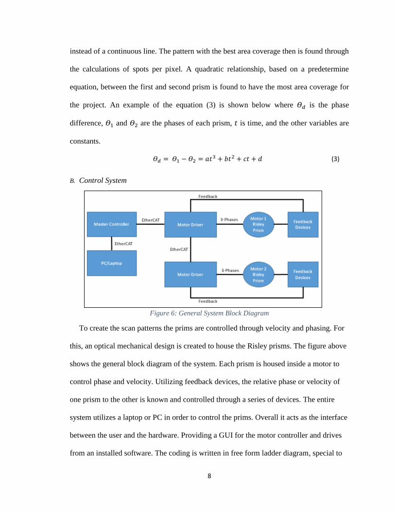
Figure 6: General System Block Diagram

To create the scan patterns the prims are controlled through velocity and phasing. For

this, an optical mechanical design is created to house the Risley prisms. The figure above

shows the general block diagram of the system. Each prism is housed inside a motor to

control phase and velocity. Utilizing feedback devices, the relative phase or velocity of

one prism to the other is known and controlled through a series of devices. The entire

system utilizes a laptop or PC in order to control the prims. Overall it acts as the interface

between the user and the hardware. Providing a GUI for the motor controller and drives

from an installed software. The coding is written in free form ladder diagram, special to

9

the system, and has an interface like LabView. Through an internet connection the PC

interfaces the master controller. Since the drives and controller have a unique IP address.

This is done either through a standard EtherCAT wired connection or remote access over

Wi-Fi.

The master controller acts as the brains of the operation and interfaces the drives. The

drives send back important information from the motors such as, velocity, winding

current, voltage, position, and other motor parameters. This gets interpreted by the

controller providing the information back to the user through the software. If the

controller receives a parameter that does not follow or match the codes instructions, error

flags are displayed. This is also the case if there is a fault on the drives such as over

current, low bus power, short circuiting, and other errors.

Through an EtherCAT wired connection the motor drives send and receive commands

and readings to and from the motors. The EtherCAT connection is daisy chained together

and all the information passes through one line. These drivers handle the actual control of

the motors, while the master controller only sends set point parameters. Additional

information on operation of the motor drivers and master control is further explained in

the design section.

The last part of the control system is the feedback devices. These parts are directly

connected to each motor driver and are used in the control loops to maintain velocity or

position. The main feedback from the motors is the hall effect sensors. Start position and

commutation are derived from these three magnetic sensors, which are positioned on the

stator to detect rotor position. Through heavy interpolation these sensors can be used for

velocity feedback during higher motor speeds. Limitations occur at lower velocities due

10

to the low resolution of feedback from three hall sensors. An encoder provides more

accurate information than the hall effect sensors and is needed for position control of the

prisms. A thermistor inside the motor provides thermal information. Although the run

time of the motor is short with a limited scanning time, the data gives an idea if there is a

fault or issue in the system. Since motor overheating is a rare case with a short run time.

C. Requirnments and Procedure

The design had a series of tasks it needed to perform, split into three phases of the

scanning process. Phase one, both motors come up to a desired speed and maintain a tight

velocity lock. Phase two, the first motor maintains the same velocity while the second

motor becomes out of phase by a certain amount relative to the first motor. Phase three,

the second motor preforms a phase difference move based on the ideal scan pattern for

area coverage. The first motor maintains the same phase and velocity while the second

motor slows and follows a phase difference equation. These are the steps the RPA needed

to run to perform the scan.

The requirements for the procedure listed above focuses on the precision of the scan

pattern and power consumption. For the first phase, the settling time for the motors to

reach their desired speeds is critical. The longer the motors take, the earlier they need to

be turned on during the decent phase. This consumes power over time from the high

speeds the motors need to reach for the scan. Although with a shorter settling times and

higher acceleration the more instantaneous power is needed. Therefore, there is a tradeoff

between the startup time and power consumption. This subject is being investigated

through simulation and demo builds to determine the best settling time versus power.

During this phase, the lock on the settling speed is also important. Variability in the top

11

speed causes errors in the phase difference between the prisms. An unsteady velocity

control causes wobble in the output of the lasers ideal position leading to missed points

and or uneven coverage on the surface.

For the second phase, when the second motor locks to an out of phase position to

motor one, the requirements are like the first phase. Again, the lock in velocity is critical

to reduce phase errors. This time the position is also a variable to consider. The lock to an

initial phase difference is to start the scanner at the widest possible point. If there was a

100 𝑚2 box, the laser would start at the edges of the box and work its way inwards. Since

the patterns are a function of time, starting at the wrong initial phase difference would

start the scan in the wrong area of the terrain. Although the scans are repeatable and

overtime the position would be filled, there is also a time consideration. Since the scanner

is limited to a couple of seconds, a misalignment in the starting phase difference causes

the scan pattern to miss an area within the terrain.

The final phase is the most important for the science portion of the project. In order to

accurately scan the area, the phasing of the second motor needs to have as little error as

possible compared to the desired equation. In addition, the velocity also needs little error

since it relates directly to the phase difference equation through a derivative. For this

portion the second motor slows to perform the phase difference. This is chosen versus

speeding up the motor due to power, torque, and control purposes. Allowing the control

to do less to maintain the tight phasing requirements.

Lastly, after the completion of the science phase the shutdown of the motors is

considered. During this time the motors are still consuming power until coming to a

complete stop. There are a couple options for this process. The motors can be shut off

12

through a hard breaking function where reverse voltage is applied to the motor for an

immediate stop. This involves the use of extra power but is the fastest way to stop

motion. Another option is reducing the power overtime and decelerating the motors. This

option offers the most control over the shutdown time but again uses power to turn off the

motors. The last option is turning off the power completely and letting the motors free

spin down to zero velocity. This uses the least amount of power but also the least amount

of control on turn off. These options are being considered and more research is needed to

decide on the best process.

IV. DESIGN

When designing IRAD projects the first step is to find commercial of the shelf (COTS)

parts that can perform the needed tasks. This allows for a rapid prototype of the RPA to be

created in a shorter amount of time. Rather than waiting for the design and testing of

driver and controller cards along with specialized motors and encoders. Using the COTS

parts also helps give insight into the control of the motors, the motor performance, power

requirements, and other aspects of the project. The control system requires a couple main

components two motors, two encoders, two motor drivers, and a controller.

A. Motor

For the motor there are a couple of different types for consideration, stepper, brushed

and brushless motors. A stepper motor provides precise and discrete steps depending on

the number of poles within the motor. Used for applications such as 3D printers, milling

machines, robotics, and more. Electrical pulses from a driver provide commutation for

each step in a specific sequence to drive the motor. Although precise positioning is need

for the prisms these motors typically operate at lower speeds and have torque capabilities

13

that fall off at higher speeds. Additionally, the stepper motor requires more power to

operate since the coils are energized constantly at maximum current draw. This leads the

stepper motor to not be a desired option for the project. The next consideration is the

brushed DC motor. These are easy to control with no commutation needed and only a

single voltage signal is used to control the speed. The main limitation with these motors is

the use of brushes that apply current through the windings as the motor rotates. This is

how control of these motors is simple, since the commutation is handled through the

brushes and a commutator within the motor. These brushes lead to a couple disadvantages

mechanical noise, brush to commutator arcing and wear, brush dust, and a shorter lifetime.

For space application these motors are typically steered away from for these reasons and

since in a vacuum the lack of a medium leads to stronger arcing. This causes the brushes

and commutator to wear out quickly and provides for poor thermal characteristics. The

final option for the RPA is a brushless DC (BLDC) motor. These motors operate with less

mechanical and moving parts than the brushed motors. Achieved through the elimination

of the brushes and having the only moving part being the rotor. Commutation is instead

done through electrical signals sent to each winding. With the difference in design, BLDC

motors can operate for longer lifetimes, higher speeds, higher efficiency and have better

thermal characteristics. These advantages are why these motors, along with stepper

motors, are the most predominant in aerospace application. Therefore, the final choice for

14

the motor type is a brushless DC motor. From knowing the type of motor that works best

for the design, research is done to find one that meets the requirements [6].

The first requirement is the velocity requirement, the motor needs to be capable of

reaching top speed for scan pattern. At this speed the motor also needs to be able to reach

this velocity with the torque load on the motor. Through calculations from knowing torque

effects from the motor, bearings, encoder, prisms, and additional loads. An estimated

torque load is used to determine if the motor can drive the full system. Then through

velocity versus torque graphs supplied from the vendor, the motor is analyzed based off

the estimated torque at a given speed. An example of one of these graphs is shown above

in Figure 7. For this example, if the top speed the motor was 6,000 RPM then the torque

load it can operate at is around 0.02 Nm.

The second requirement is power, the motor must utilize as little power as possible

during acceleration and top speed. In order to determine the power that is used for the

scanner, a couple of parameters are used. The speed in which the scan happens gives

insight into the max voltage that the motor runs at. This is done through checking

datasheets on each motor to find the back EMF constant. Since in BLDC motors an

Figure 7: Torque Velocity Example [7]

15

energized stator powers the rotation of the rotor, this causes an induced AC voltage in the

rotor. The effects of which are determined through measuring the output terminal voltage

of the motor at certain speeds. This measurement is a constant dependent on velocity that

is expressed as back EMF. From knowing the opposing voltage of the motor at a given

velocity, in order to cause rotation, the motors input voltage is estimated slightly higher

based on the constant. For example, if the back EMF constant is 17 𝑉/𝐾𝑅𝑃𝑀 and the

motor is driven at 1,000 𝑅𝑃𝑀the input amplitude voltage needs to be greater than 17 𝑉.

To estimate the current on the motor the torque constant is used. From calculating the

estimated torque load on the motor, this constant is used to represent the produced current

based on the generated torque. Since the motor drives the torque load, an estimated current

is derived. For example, if there is a 0.5 𝑁𝑚 load with a motor constant of 0.15 Nm/A an

expected current of at least 3.33 A is needed to rotate the motor. Based off these

calculations an estimated max operation power of the motor is derived.

The last requirement focuses on the dimensions and weight of the motor. Since the

eventually goal of the project is to position the RPA on a lander, these are critical

parameters. A large and heavy motor assembly adds weight and in turn fuel cost to the

lander. Therefore, when considering the motors, the smaller, lighter sized the better.

Additionally, the setup requires the motor to hold the Risley prims and have a laser

pointed through them. This requires a special type of BLDC motor called a frameless

motor. These operate the same as normal BLDC motors but have rotor and stator

components not fixed in a standard motor housing. Meaning they don’t include an output

shaft or shaft support bearings. Instead where the output shaft normally is there is a hole of

a certain diameter. This diameter is dictated based on the needs of the project. The larger

16

the diameter the more feedback light from the laser is collected. For landers with a low

light reflective surface a larger diameter is required and for high reflectivity a smaller

diameter is required.

From these requirements a couple motors were chosen which met the standards for the

RPA design. For the rapid prototype a frameless BLDC WYE configured COTS motor is

selected with hall effect feedback included in the stator assembly and temperature

feedback through a thermistor. For the demo motor housing was created to fix the stator

and rotor in place. Additionally, a couple of L-brackets were used to hold the motor fixed

on a tabletop to reduce vibration. The housing was grounded to earth ground to reduce

magnetic effects and to insulate the motor. Wiring of each motor was split into two

sections, the winding power and feedback paths. These lines were both shielded in a

conductive sleeve, that is also wired to ground to prevent electromagnetic interference

between the feedback and 3-phase power lines, thus reducing noise. By creating a rotor

Figure 8: Mounted Demo Motor

17

cap, the prisms were mounted and glue on the ends of the motor. The final step positioned

and mounted both motors next to each other, so the prism were close together. An image

of the assembly for one of the motors is shown in the figure above.

A secondary COTS motor is also selected with the same BLDC configuration and

meeting the requirements. This motor fit the design of the project closer than the demo

motor. With the dimensions and weight being almost half the size. The motor also had

lower power requirements at the top speed of the scanner and a zero cogging torque which

reduced the torque effects on the motor. Since this motor was a custom design from the

vendor it has a long lead time for construction. Therefore, the demo motor that fit the

requirements is used in place of this motor. The tradeoff being that the control of the demo

motor is based only on hall effect feedback. Instead of spending resources, when a more

adequate motor is being built, the encoder selection focuses on fitting the second motor.

Utilizing the first motor while the second was being built gave insight into the drives,

control, and operation of the full system.

B. Drives and Controllers

After the selection of a brushless DC motor, a drive system is determined. Since the

lack of a commutator in these motors requires more complex drive circuity a couple

different COTS drivers and controllers are examined. With the progressive advances in

machine automation for assembly lines, autonomous robots, and other automated systems

there is many new advances in commercial controllers. These systems have already been

tested for plastic injection molding, glass printing, labeling machines, and even a virtual

reality roller coaster system. To evaluate these systems, the controllers and drivers need to

18

be capable of operating the RPA under each phase of the procedure and meet

requirements.

The main requirement is the ability to operate the BLDC motors with the needed power

and control performance for the scan. For this, the power calculations in the motor design

section give insight into the needed output drive power. Based on the calculations a driver

with the capabilities to provide this power is chosen. For control performance the motors

need to maintain the smallest error in terms of velocity and position. This means the

drivers update rate and feedback resolution are an important feature. The update rate

provides insight into the performance of the control loops in the system. A slower rate

may not be able to maintain the precision needed for the velocity and phase lock for the

motors. Also, the feedback resolution of the drives is another factor that adds to the error

in these parameters. A system with a high interpolation factor and sampling rate is optimal

for better control.

From these requirements a commercial controller and two motor drivers are selected.

The drivers operate off either AC or DC to power the internal H-bridge circuitry. Then

with the control logic, pulsed 120° sine wave commutation is sent to each phase of the

motor. Based on the max and min duty cycle of the pulsed commutation the output voltage

levels are controlled. This type of commutation offers the lowest torque ripple for the

motors and is typical for a higher performance system. Each drive either operates off

torque, position, or velocity control. For the initial demo only hall effect feedback is used,

and the drive only operates with velocity or torque control. Since the drivers operate and

control each motor individually an additional master controller is used. This gives the

ability for multi-axis control based on relative position or velocities between the two

19

motors. Through an EtherCAT connection, with a 4 kHz update rate, the controller can

command position, velocity, or torque of each control loop at a given time. Feedback from

each driver gives the controller information on the current status of each motor. Then

through a program coded within the controller the memory within each driver is updated

with the needed value. Details into the control system used for the project and coding are

explained in the control section.

Figure 9: Controller and Driver System

The drives and controller are mounted together in a rack and wired as shown in the

figure above. A main 120 V AC line is used to power each of the H-bridges for the drives.

An additional 24 V line is used to power the master controller and control logic for the

motor drivers. These controllers and drivers are insulated through a chassis ground to earth

to reduce electromagnetic interference between them. For communication EtherCAT

wires are connected in series between the drives and controller. A network switcher is

used to provide connection between the system, router, and computer. Then through either

a hard wired connection or remote access the master controller and drives are configured

and programmed for the project.

20

C. Encoder

The selection for the encoder is based on a few requirements and design constraints.

For the design, the engineer can base the best option for the RPA on the parameters of

encoder type, resolution, accuracy, and dimensions. The output of the encoder is used for

position feedback for the motors and as data points for the detector. In order to create a

detailed map of the terrain a minimum resolution for the encoder is based upon the needed

resolution for the detector. For the maximum resolution the update rate of the control and

the maximum speed of the motors for the scan are examined. Since the controller has a

given clock rate for the feedback and the motor spins at a certain frequency, the controllers

clock limits the maximum resolution. For example, consider the feedback rate of the

controller is 1 MHz and the motor spins at 5,000 RPM for the scan. This means the

controller reads at a rate of 1 μs while the motor completes a revolution every 12 ms.

Using these calculations, the maximum number of samples per revolution is 12,000 then

converting the value to a bit resolution the max is ~13 bits. Therefore, using these

numbers and calculations, the maximum and minimum resolution of the encoder are

determined. The accuracy for the encoder sets the error based on the true position of the

motor being measured and the position reported by the encoder. This value does not relate

to the resolution of the encoder and is typically measured in arcseconds or microns based

on the type of encoder. Since the value represents the error for the encoder, the smaller the

value the better.

The next limitation for the encoder is the dimensions and type. Since the BLDC motors

for the project are frameless, with the ability to have a laser shined through the center, the

encoders cannot block the prisms output. Therefore, the mounting of the encoders is

21

positioned on the rotor with a bore equal to or greater than the bore of the motor. The size

of the outer diameter for the encoder leads to the maximum diameter of the RPA. A

smaller encoder leads to a smaller housing which makes the dimensions of the encoder

critical. The type of encoder is based on the needs for the prism. Since the absolute

position of the prims are needed for the control of the scanner and detector feedback, an

absolute encoder is more viable. On the other hand, an incremental encoder bases its’

measurement in relation to a starting point. Which means each time the system is turned

on a new starting point is used for reference that does not dictate the starting position of

the prisms. Therefore, the absolute encoder is the preferred choice for the RPA. The final

choice for the encoder is chosen based on the environmental requirements. Since in most

space application a general concern is radiation and magnetic interference which adds

noise to the system and causes shorter lifetimes. For the project one potential mission is a

highly radiate and magnetic environment. Therefore, an optical encoder is of more benefit

than a magnetic encoder which would provide for a less noisy signal in an extreme

environment. Since optical encoders are still affected by radiation the selected encoder

must have rad hard capabilities. The encoder is also mounted in a surrounding housing to

prevent additional radiation effects. A final rad hard, absolute optical disk encoder is

chosen for the RPA.

V. CONTROL

A. Velocity Loop

In order to control the motors a few things had to be taken care of. The first of which is

setting up the motor drivers control loops for system performance. The COTS drive used

in the RPA design had a couple different operation modes torque, velocity, or position.

22

Each had its own unique control loops with filters, PIs, limiters, feedforward, and other

control options. These parameters for the drive are edited through user input. An auto

tuning function is also available for the control loops but when utilizing hall effect

feedback only, the auto tuning is not available. Therefore, tuning of the system is done

based off the main criteria, velocity.

The general block diagram for the velocity control loop is shown in the figure above.

Using the feedback from the hall effect sensors and an ideal velocity command, the

control system outputs a current onto the motors to produce movement. Since the hall

feedback is heavily quantized, to be used for velocity, large current spikes occur at each

transition points. The unedited velocity feedback from the system appears as a series of

random impulses due to the current spikes and an exact value cannot be determined. In

order to filter the noisy signal an observer and a set of anti-resonance filters, represented

by AR, are used. The observer, also known as a state observer, is used to estimate the state

of a given system through measuring the input and output of the full system. For example,

if a car enters a tunnel the speed and position the car enters and exits are known by the

observer. Then from this knowledge an estimated position and speed within the tunnel at a

given time can be mapped. In this case, by knowing the input and output current command

an estimated velocity is generated from the observer. This signal is filtered within using a

low pass filter to reduce the noise before use. After the observer another series of filters

Figure 10: General Control Block Diagram

23

are also need. Each AR is capable of being either unity gain, low pass, biquad, notch, or

lead lag. Since the output signal from the observer sill presents noise in the system two

low pass filters are added. This provides a clean velocity feedback signal that is then used

to determine the error based on the velocity command. First a ramp limiter is used which

sets the max acceleration for the motors. The velocity command is then limited by the max

output velocity set by the user. Which is determined through max velocity limitations of

the motor. A generated error signal is then able to be filtered through AR1 and AR2. A

single low pass filter is used to reduce noise in the error signal with a lower quality factor

than the velocity feedback filters. The error signal then is controlled through a PI system

to produce the current command on the motors. Exact tuning for the PI system is done by

hand since the auto tuning function is unavailable when using hall feedback. The

performance of the tuning is evaluated through the percent error between the commanded

velocity and velocity feedback from the hall sensors. Results of the performance of the

control system are shown in the results section of the project.

24

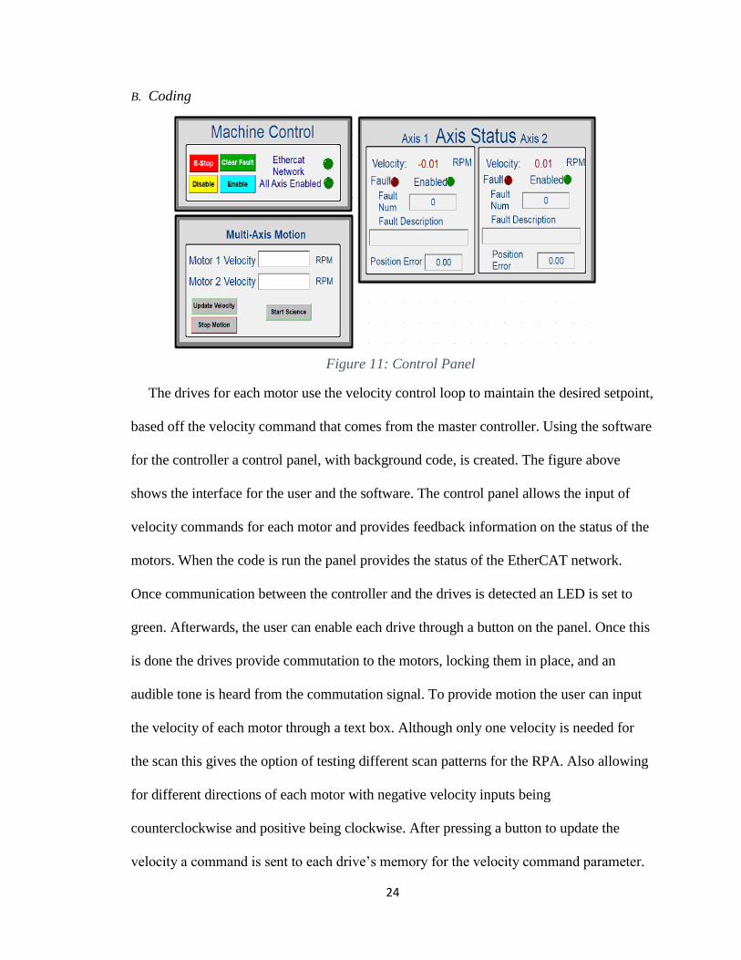
B. Coding

The drives for each motor use the velocity control loop to maintain the desired setpoint,

based off the velocity command that comes from the master controller. Using the software

for the controller a control panel, with background code, is created. The figure above

shows the interface for the user and the software. The control panel allows the input of

velocity commands for each motor and provides feedback information on the status of the

motors. When the code is run the panel provides the status of the EtherCAT network.

Once communication between the controller and the drives is detected an LED is set to

green. Afterwards, the user can enable each drive through a button on the panel. Once this

is done the drives provide commutation to the motors, locking them in place, and an

audible tone is heard from the commutation signal. To provide motion the user can input

the velocity of each motor through a text box. Although only one velocity is needed for

the scan this gives the option of testing different scan patterns for the RPA. Also allowing

for different directions of each motor with negative velocity inputs being

counterclockwise and positive being clockwise. After pressing a button to update the

velocity a command is sent to each drive’s memory for the velocity command parameter.

Figure 11: Control Panel

25

While in motion an axis status section provides the user with the velocity readings of each

motor and any faults detected on the drive. Once the desired speeds of the motors are

reached the user can start the scanning processes at any time from the start science button.

The scanning process is velocity difference controlled with the first motor holding the

same velocity and the second motor slowing to perform the needed phase difference of the

prisms.

The control panels input and output variables as well as buttons and LEDs are tied to a

background code that controls the system. A general block diagram shows an overview of

the process the code takes. For the program three scripts are integrated together, main,

triggers, and math section. The main section handles the higher level control like velocity

commands, initialization, axis status, and motor readings. Triggers handles the sub level

control of timers and flags for the system. Math takes care of data conversion and details

the scanning equation in terms of velocity. The first part of the program is initialization,

here the motion library for the code is stated for the compiling of the program. Since the

Figure 12: Software General Block Diagram

26

controller can be coded using a couple different languages all unique to the controller.

Once the library is imported into the software the EtherCAT lines are cleared. Each axis is

then assigned a variable that can be used in the code, tied to a specific drive. After the

initialization the program enters a conditional statement based on the enabling the drives

from the user. If the drives are enabled from the button on the control panel, the system

enables power to each of the motors. Power is then disabled if the user presses an

emergency stop button or disables the drives anytime during the program. In the event of

an emergency stop the controls output a breaking reverse current which immediately stop

the motors. In any other case the motion is slowed through a deceleration function

controlled from the users input.

The code, within main, then comes to two write to memory functions. These functions

are set up to write the specific velocity value to the velocity command parameter within

the memory of each drive. The value is command based on the EtherCAT slave address,

memory index and sub index within the system. This function executes only when the user

presses the update velocity button on the panel. The input into the text box on the control

panel is converted into a usable value from the math section. Since the memory requires

the velocity value to be defined in 1,000 of RPM. Acceleration of the motors is controlled

through a parameter defined in the drive’s setup.

Once in motion the main code uses two memory read functions to display the value of

the velocity feedback parameter within each drive. The function works like the write to

memory command using the EtherCAT address and memory index for the value. Since the

functions are single executes a clock signal is created within the triggers section of the

code. This function outputs a pulse wave modulation signal from zero to one based on the

27

desired speed of the function. The max clock speed is used to get a constantly updated and

reliable value that is output to the control panel for the user. The math section again

converts the value to a readable RPM before output.

For the scanning portion of the project the start is controlled from the user pressing the

start science button on the control panel. Once this occurs the trigger section executes a

timer that measures the elapsed time since the button has been pressed. Through the math

section it is converted into a usable variable that can be input into a velocity difference

equation. Since the motors for the demo are operating in a velocity mode instead of the

ideal position mode, the phase difference equation is converted. This is done through

taking the derivative of the ideal position equation to get velocity. Then within the math

section, it is created through a series of functions that use the converted time as the

dependent variable. To account for system error an additional constant is added to the end

of the equation. The value of which is determine through trial and error based on the

required scan time. An ideal scan time of a couple seconds is defined by the project

requirements, this is the determining factor for the additional error. The output of the

equation is the velocity difference between each motor. Therefore, this value is subtracted

by the current velocity of the first motor and is output to a new write to memory function.

Since these functions are single executes, the clock signal defined in the triggers section is

used to continuously update the memory. Once the scan reaches a certain time, input from

the user, the triggers section sends a flag to main. This flag then commands each motor to

decelerate based on initial setup. When the motors reach no motion the final stage of the

RPA has finished.

28

VI. SCANNER SIMULATION

A. Overview

In order to understand the construction of the scanner, project teams developed a

couple simulations. These gave expectations on parameters from the design that aided in

construction of the project. For the RPA important information can be determine from

simulating the control system for the motors. Some outputs that the simulation provides

are winding voltages and currents, torque, velocity, motor phasing and more. Of these the

phasing information can be sent to the optical to teams’ simulation to helped determine

features like pixel per spot coverage. Since the optical simulation provide more

information on the detector and laser for the scanner.

The creation of the RPA sim focused on modeling the full system through motor

drivers, motors, and an encoder system for position feedback. Utilizing MATLAB, the

simulation shown in the figure above is created. The full system operates each of the three

phases listed in the procedures. For the first phase the drives are commanded through a

ramp function based off the ideal acceleration of the motor. This function is limited

through a saturation block to a desired settling speed. The second phase uses a phase

Figure 13: MATLAB RPA Simulation

29

difference input equation into the second motor driver. Then based off the feedback from

the first motors encoder, the ideal position is commanded to the second motor. Once a set

time is reached, defined by the user, the phase difference equation outputs the motor

position over time for the scan pattern. When the scanning period is complete the

simulation is ended, and an output of the scan pattern is show to the user. Parameters for

the drives and for the motors are controlled through user input from a script file.

Additional outputs are also controlled and collected through the same script.

B. Motor Drivers

Figure 14: Simulation Motor Driver 1

Two motor drivers are created to control identical motor systems with one being a

slave to the other. The first motor drive controls and executes all the steps for the first

motor. Inputs for the drive include the desired speed of the scan, current speed of the

motor from the encoder, and encoder motor shaft position. With these inputs a velocity

control loop is created and a PID system maintains the output voltages onto the three

phase motor windings.

To simulate the drives picked during the brainstorm process of the design phase a

couple of attributes were used. The first of which is the output of sinewaves to mimic the

COTS drives. This is done through utilizing the feedback from the encoders motor shaft

position. A quantized and sampled shaft position that when scoped forms a sawtooth

30

waveform from 0 to 2π. Based on the motors shaft position the drive calculates the needed

commutation sequence to move the motors. Typical sinewave commutation uses three

signals offset by 120° or 2𝜋

3 radians. Therefore, each phase has an addition of this offset,

phase A +0 radian, phase B + 2𝜋

3 radians, and phase C +

4𝜋

3 radians. Using this

information, the drive can output commutation for one electrical cycle of the motor. In

order to operate a full rotation, the number of poles in the motor is also considered for the

electrical cycles. As a gain function, the number of cycles is multiplied by the motor shafts

modulated position, giving the drive the ability for complete rotations. The equation (4)

below represents how the drives calculate the commutation signal for each phase of the

motor. Where SP is the motor shaft position from 0 to 2π, EC represents the electrical

cycles, and the values of which are assumed to be radian values. The output of the sin

function is a signal that oscillates between zero to one depending on these values.

𝑃ℎ𝑎𝑠𝑒 𝐴 = 𝐴 ∗ sin(𝑆𝑃 ∗ 𝐸𝐶) (4)

𝑃ℎ𝑎𝑠𝑒 𝐵 = A ∗ sin(𝑆𝑃 ∗ 𝐸𝐶 +2𝜋

3)

𝑃ℎ𝑎𝑠𝑒 𝐶 = A ∗ sin(𝑆𝑃 ∗ 𝐸𝐶 +4𝜋

3)

31

For the sinewaves to produce a voltage to drive the motors, the output of the equation is

also multiplied by A, the amplitude of the signal from the control loop. The first motor for

the scan, only needs to come up to a velocity and hold. Therefore, a velocity control loop

is used to generate the voltages on the motor. Using the desired speed input from the user

and the current speed, read from the encoder system, an error function is created through

the subtraction of the two. The error feeds into a PID control block that outputs the voltage

amplitude. Each PID in the simulation is tuned to a specific need. For motor one the

important parameter is velocity. Therefore, the PID is tuned based on quickest settling

time and lowest velocity error using a MATLAB auto tuner and additional hand tuning

afterwards. To also represent the control system the PID is run in discrete time based off

the update rate of the motor drives. Limitations are also set on the amplitude of the output

voltage to ensure the output is never more than the driver can supply. Finally, in

representing the motor drives, the output commutation is quantized based off the output

resolution.

The secondary motor drive operates differently compared to the first drive since its

procedures are more complicated. Motor 2 needs to operate the same as motor 1 during

the first phase by coming up to a desired speed. But in phase 2 and phase 3 the second

Figure 15: Simulation Motor Driver 2

32

motor has a phase difference requirement to start and preform the scan pattern. The inputs

for the driver are the same as the first with the addition of a desired relative phase and

position of motor 1. End goal is again the same with motor shaft position being used to

determine the commutation output at a certain voltage. This voltage is determined by two

different control loops a velocity loop and a position loop.

During the first phase of the simulation the velocity loop is used to get the motor up to

speed. The same PID tuning, update rates, and voltage limits are used as in the first motor

driver. An additional trigger is added to switch between this loop and the position loop.

Once the speed of the motor is detected to have reached the settling velocity the switch

occurs. The time when this is triggered is saved as a variable to be used to know how fast

the motors came up to speed. Utilizing a switch between the two loops is done for

stability. When the two loops are cascaded, velocity and position, the two functions fight

each other and cause oscillation. Additional ringing is noticeable in the second and third

phases in the position of the motor. This also emulates the control of the drives which

utilize different control loops in order to drive the motors, a position, velocity and torque

loop.

33

C. Motor

The motor system for the simulation is controlled by the motor drives through the

voltage output commands. This system is split up into two different function blocks, a

winding model and a mathematical model that represents the motor. The motor windings

input the voltage commutation from the drives, and the back EMF from the math section.

Outputting phase currents based on the resistance and inductance of the motor. Which are

used to generate motion from the calculations block. Parameters are then calculated from

these currents such as motor velocity, torque on the motor, winding current, shaft position

and more. Representation of the motor focused on a brushless DC WYE configuration,

since it was the optimal choice in the design phase. There are a couple assumptions that

are made in order to reduce the complexity of the model. Which are, no magnetic

saturation, no hysteresis and eddy current losses, uniform air-gap, no mutual inductance,

and no armature reaction.

Each phase of the motor is represented in circuit form within the winding model.

Utilizing resistors for the line to line resistance and inductors for the line to line

inductance. These values are divided in half since each phase is modeled based on the line

Figure 16: Simulation Motor Model

34

to neutral form for easier representation in the simulation. A single series resistance and

inductor to a zero point serves as one line of the windings. The zero point is a function

solver that ensure the neutral point of the motor is always at zero. Then the calculated

sinewave voltage is injected across each phase of the motor. In opposition, a back EMF

signal generated from the calculation section that opposes the commutation signal. The

total voltage across the winding is calculated from the equation shown below (5). Where R

represents line resistance, e is the back EMF, 𝑖𝑛 is the line current and L is line

inductance.

𝑉𝑎 = 𝑖𝑎𝑅 + 𝐿𝑑𝑖𝑎

𝑑𝑡+ 𝑒𝑎 (5)

𝑉𝑏 = 𝑖𝑏𝑅 + 𝐿𝑑𝑖𝑏

𝑑𝑡+ 𝑒𝑏

𝑉𝑐 = 𝑖𝑐𝑅 + 𝐿𝑑𝑖𝑐

𝑑𝑡+ 𝑒𝑐

A current sensor is used on each of the phases to measure the value of the line current.

The measured value is sent to the calculations section to determine the generated

electromagnetic torque of the motor. This is done through utilizing the back EMF constant

since in practice it is equal to the torque constant of the motor. The torque constant of the

motor is given in 𝑁𝑚 𝐴⁄ and describes the relationship between the motor current and

generated torque. By multiplying the constant times each of the phase currents and

summing the results, the total torque is found. This is done in the form of back EMF that

is re-injected into the windings of the motor and additional information is shown later.

The generated torque of the motor is then used to determine the acceleration, speed,

and position of the motor shaft. On the motor there is always an opposing torque that is

35

represented through a subtraction function from the generated torque. Here parameters

such as viscous damping, bearing friction, cogging torque, and static friction are

represented. The static values are simply created as addition to the applied torque on the

motor. Values like viscous damping are created through a gain function based off the

speed of the motor since it is a function of velocity, viscous damping = 𝑁𝑚 𝑅𝑃𝑀⁄ . For

cogging torque, the function depends on the position of the motor and represents the

effects between the rotor and stator slots of the permanent magnets within the motor. By

multiplying the motor shaft position, electrical cycles, and putting it through a sin function

the position of the cogging is calculated. Then through a gain function the cogging torque

value is represented from the multiplication of the result position. These values are all

summed together to oppose the generated torque and the subtraction forms the

acceleration torque.

𝐴𝑐𝑐𝑒𝑙𝑒𝑟𝑎𝑡𝑖𝑜𝑛 = 𝐺𝑒𝑛𝑒𝑟𝑎𝑡𝑒𝑑 𝑇𝑜𝑟𝑞𝑢𝑒−𝑂𝑝𝑝𝑜𝑠𝑖𝑛𝑔 𝑇𝑜𝑟𝑞𝑢𝑒

𝐼𝑛𝑒𝑟𝑡𝑖𝑎 (6)

Through the following equation above (6), the acceleration of the motor is calculated

utilizing the inertia, generated torque, and torque on the motor. From the calculated

acceleration value, the speed and position are also determined by taking the integration of

each value. For acceleration the integration brings velocity, and from velocity the

integration brings position. The output of the position function is a continuous phase

profile. For the variable to be used as the motor shaft position the output is modulated

from 0 to 2π. The speed is also output from the model and is used in the viscous damping

and back EMF calculations.

36

The last part of the calculations section is to generate a back EMF voltage across the

motor and for the torque generation. Since the back EMF signal is controlled through

position the output from the integration of the acceleration is used. This value is multiplied

by the electrical cycles for position and passed through a sine function. For commutation

each phase is offset by 2𝜋

3 radians and then multiplied by the back EMF constant. To

generate back EMF the output is multiplied by the current speed of the motor. Since the

constant is given in 𝑉 𝑅𝑃𝑀⁄ the final output is a voltage that is sent to the winding model.

To generate the torque from each phase current, instead of multiplying by velocity to get

back EMF, the function is multiplied by each phase current. The following equations (7)

(8) show how each of the functions are calculated where the first three are for each back

EMF per phase and the last is the torque generated. The F(x) represent the sinewave

function generated in the model, 𝑒 is the back EMF voltage, ω is for velocity in rads/s, 𝑖 is

for current, and 𝐾𝑒 is for the back EMF constant.

𝑒𝑎 = 𝐾𝑒 ∗ 𝐹(𝑥) ∗ 𝜔 (7)

𝑒𝑏 = 𝐾𝑒 ∗ 𝐹 (𝑥 + 2𝜋

3) ∗ 𝜔

𝑒𝑐 = 𝐾𝑒 ∗ 𝐹 (𝑥 +4𝜋

3) ∗ 𝜔

𝑇𝑒 =𝑒𝑎𝑖𝑎+𝑒𝑏𝑖𝑏+𝑒𝑐𝑖𝑐

𝜔 (8)

D. Encoder System

The modulated output from 0 to 2π of the motor shaft position is further used in the

control system. An encoder model is created to represent a simulated encoder based off

specifications from the design. For this encoder, the modulated shaft position is quantized

37

based on the resolution of the encoder. Additional quantizing is also added here based

extra interpolation from the motor drives or an extra interpolation box. To also represent

the drives after quantizing the position the value is also sampled at the rate of the drive.

This allows the system to output values that are closer to the actual encoder. Three outputs

come from the encoder system an encoder speed, encoder shaft phase, and an encoder

phase profile. The encoder speed represents the calculated velocity that feeds directly into

the drive for the velocity control loop. The phase profile is used to make a continuous

representation of the position of the motor and is used to feed the second motor driver as a

slave. The last output is the encoder shaft phase which is a modulated and quantized

position that is feed into the drive. Used to calculate the commutation in order to drive the

motors.

E. Phase Equation

The last part in the control model simulation is the phase equation for the Risely

prisms. It is used to determine the ideal phase difference of motor one to motor two and is

needed for phase one and phase two of the scan procedure. The module works through a

cubic equation formed form a series of MATLAB blocks. A time variable is used as the

input to pass through the equation which represents the passing time of the simulation.

The time variable is first delayed by an amount of time set through user input. This delay

marks when the RPA starts the scanning process. Before the delay, the time variable is

zero and only the constant of the cubic equation is output. The constant represents the

phase difference needed for phase two of the RPA project. Which is used when the motors

reach the desired settling time and the switch of the second motor driver is triggered for

the position loop. After the set delay time from the user the phase difference equation is

38

initiated and the time passing through increases from zero. The cubic equation then

outputs the ideal phase difference to perform the scan. After a couple of seconds or a time

defined by the user the simulation stops and the scan pattern and other outputs are

displayed.

F. Simulation Script

Behind the MATLAB simulation model there is a control script that is used for

variables and outputs. The user can input parameters regarding the brushless motor like

back EMF, line resistance, line inductance, viscous damping, and others. Additional,

parameters for the other aspects of the simulation like science start time, encoder

resolution, driver limits, acceleration limits, desired speed, and more are defined here.

After the initialization of these variables the script runs the MATLAB Simulink model for

the RPA. Then through a series of MATLAB functions certain parameters like speed,

phase profile, phase difference and more are output in graphs once the simulation is

complete.

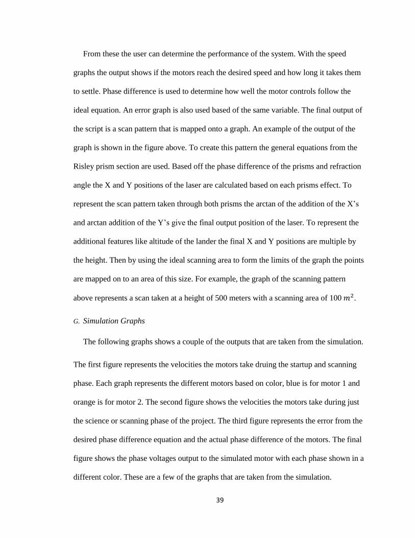
Figure 17: Simulated Scan Pattern

39

From these the user can determine the performance of the system. With the speed

graphs the output shows if the motors reach the desired speed and how long it takes them

to settle. Phase difference is used to determine how well the motor controls follow the

ideal equation. An error graph is also used based of the same variable. The final output of

the script is a scan pattern that is mapped onto a graph. An example of the output of the

graph is shown in the figure above. To create this pattern the general equations from the

Risley prism section are used. Based off the phase difference of the prisms and refraction

angle the X and Y positions of the laser are calculated based on each prisms effect. To

represent the scan pattern taken through both prisms the arctan of the addition of the X’s

and arctan addition of the Y’s give the final output position of the laser. To represent the

additional features like altitude of the lander the final X and Y positions are multiple by

the height. Then by using the ideal scanning area to form the limits of the graph the points

are mapped on to an area of this size. For example, the graph of the scanning pattern

above represents a scan taken at a height of 500 meters with a scanning area of 100 𝑚2.

G. Simulation Graphs

The following graphs shows a couple of the outputs that are taken from the simulation.

The first figure represents the velocities the motors take druing the startup and scanning

phase. Each graph represents the different motors based on color, blue is for motor 1 and

orange is for motor 2. The second figure shows the velocities the motors take during just

the science or scanning phase of the project. The third figure represents the error from the

desired phase difference equation and the actual phase difference of the motors. The final

figure shows the phase voltages output to the simulated motor with each phase shown in a

different color. These are a few of the graphs that are taken from the simulation.

40

Figure 19: Motor Simulated Velocity Profiles

Figure 18: Motor Simulated Scanning Velocities

41

Figure 21: Simulated Phase Error Profiles

Figure 20: Simulated Phase Voltages

42

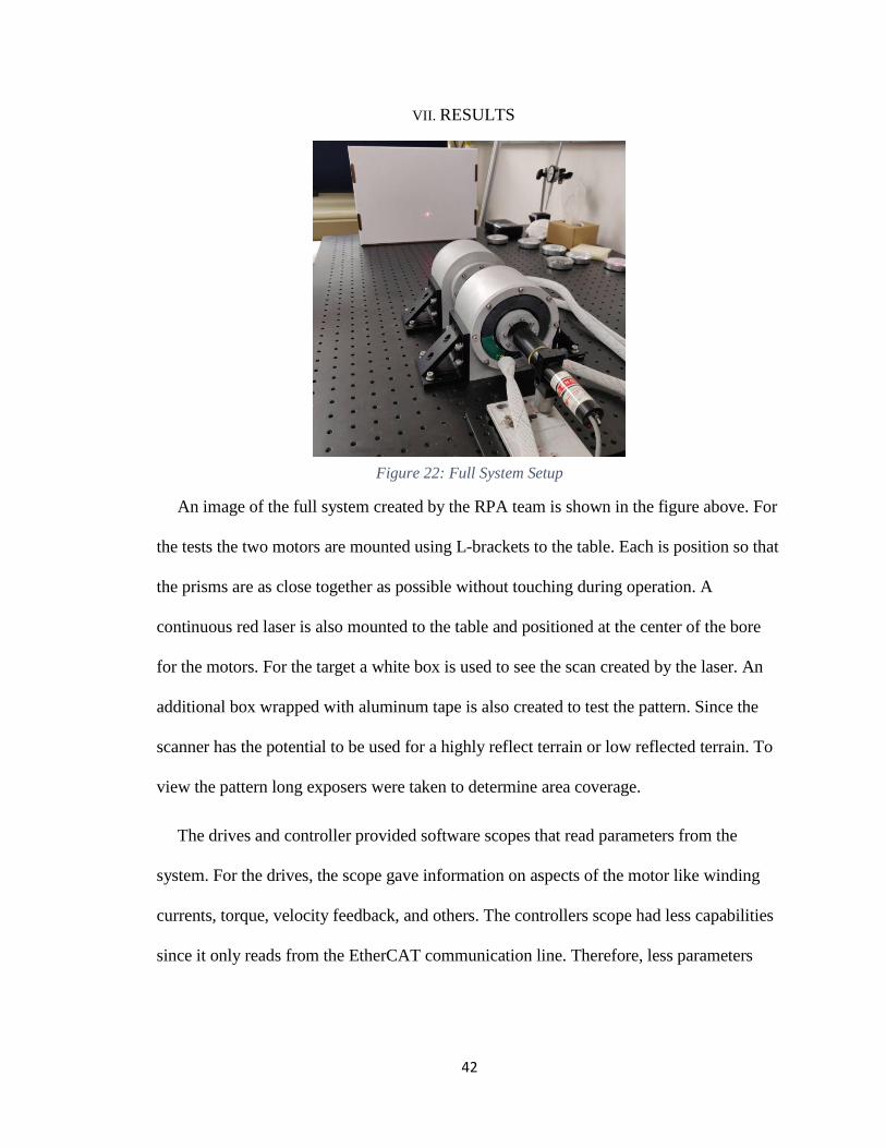
VII. RESULTS

An image of the full system created by the RPA team is shown in the figure above. For

the tests the two motors are mounted using L-brackets to the table. Each is position so that

the prisms are as close together as possible without touching during operation. A

continuous red laser is also mounted to the table and positioned at the center of the bore

for the motors. For the target a white box is used to see the scan created by the laser. An

additional box wrapped with aluminum tape is also created to test the pattern. Since the

scanner has the potential to be used for a highly reflect terrain or low reflected terrain. To

view the pattern long exposers were taken to determine area coverage.

The drives and controller provided software scopes that read parameters from the

system. For the drives, the scope gave information on aspects of the motor like winding

currents, torque, velocity feedback, and others. The controllers scope had less capabilities

since it only reads from the EtherCAT communication line. Therefore, less parameters

Figure 22: Full System Setup

43

were able to be recorded but the additional data came directly from each drive. Using this

feature the RPA is evaluated based on the requirements of the project.

A. Performance

To measure the performance of the system a couple of parameters were evaluated

based on the requirements of the project. Since the demo build used hall effect only

feedback, the main parameter to create the scan is velocity instead of the ideal position.

Therefore, the first criteria examined is the velocity control of the system. The velocity

control loops within the drive affects the overall performance to maintain a given velocity

set point. As mentioned in the controls section the loop is tuned to give as little error as

possible. Utilizing the scope within the drive the parameter of velocity feedback can be

graphed versus time. Each measurement is taken within a couple second time period

which is the same as the scan time of the RPA. Using the scope, average, maximum,

minimum, RMS, and peak to peak values are recorded. For the velocity the maximum

error represents how well the control system maintains the commanded velocity from the

controller. The following graph above shows the performance of the control loops in an

error percentage versus speed.

0

0.5

1

1.5

2

2.5

0 500 1000 1500 2000 2500

Erro

r (%

)

Velocity (RPM)

Peak Velocity %Error Vs Velocity

Figure 23: Velocity Error Vs. Velocity

44

The graph represents the maximum percent error per each velocity reading. A series of

input velocity commands were given to the drives and the feedback was measured after

the motor reached the final speed. Using the maximum reading, a percent error is

calculated based on the ideal velocity. At higher speeds the control system can maintain

the desired velocity at a maximum percent error less than 0.5%. At lower velocities the

control system has difficulties maintaining the same rate. This is due to the use of hall

effect only feedback. Since the resolution from the three hall effect sensors is too low to

give an accurate reading from the motors at low speeds. The controller company provides

an estimate from a manual for how low the system can maintain the same rate of speed

using this feedback. For example, the drives receive a new position by the hall effect

sensor every 60° based on the electrical cycles of the motor. A motor with 6 pole pairs

per revolution is 3 electrical revolutions, which leads to a hall position every 20°. This is a

low resolution that provides difficulties for the drives. From the manual the limit on

control comes from the hall effect frequency and motor poles. For the system used in the

project the limit on control is found to be about 250 RPM utilizing hall only feedback. This

is seen from the graph where the error rate around 250 RPM is close to 2% and after

increasing speeds the error percentage drops. When running the motors at a velocity

lower than this the revolutions are no longer a clean rotation and jerk. The

measurements taken provide information on the performance of the control system and

validate the limits for velocity control using hall only feedback.

45

The second important requirement for the system is power. In order to measure the

power consumed by the drives and motors a DC power supply is used in place of the 120

V AC supply. This makes it easier to measure the power consumed since the DC power

supply displays the voltage and current usage. The graph above represents the power used

over a series of different velocities for a single motor. Since the motor accelerates to reach

and maintain a certain speed. The series of measurements give information on the power

used for startup and final speed. In the orange the recorded readings come from the DC

supply, blue is an estimate from the motor windings, and grey is an 80% efficiency

estimate from the motor. The difference between the motor power and power supply give

insight into the efficiency of the power supply. From the graph it is seen that the

difference between the supply and motor are generally consistent.

For the motor power, the winding currents and voltages were measured. The drives

scope allows for the winding currents of each phase of the motor to be graphed. Each

measurement is taken over a couple second time period and recorded to a CSV text file.

0

10

20

30

40

50

60

70

200 700 1200 1700

Po

wer

(W

)

Velocity (RPM)

Power Vs. Speed

MotorPower

PowerSupply

80%Efficiency

Figure 24: Power Vs. Speed

46

To validate the measurements taken from the drive an additional external current probe is

used. The probe measured the current on a single winding and the scope results are

compared to the drives scope. The values of each matched and for simplicity the data

taken from the drive is used. Since it provides information on maximum, minimum, RMS,

peak to peak and more.

To measure the winding voltages a single phase of the motor is scoped from an external

oscilloscope. The drives output 120° sinewave commutation in the form of pulsed sine

waves. Therefore, the oscilloscope displayed a series of pulses at a frequency around 8

kHz that ranged from pulse or minus the H-bridge supply voltage. To determine the actual

voltage on the windings the scope probe measures from neutral to a single motor line. This

is done through using the DC power supply ground as the reference point. Then using the

scope, the maximum and minim duty cycles of the pulsed train give the value of the

voltage on the windings. For example, if the H-bridge is powered by 100 V the pulses

would have an amplitude equal to this value. Then at a certain speed the max duty cycle is

measured to be 52% and the minimum is measured at 48%. A peak voltage of 52 V and

minimum voltage of 48 V is calculated, the difference of which represent the peak to peak

voltage of 4 V on the winding. This value is then used along with the current readings to

determine the power the motor uses. It is also converted to phase voltage since the

measurement represents the line to neutral voltage.

The power calculation is based off the total three phase power since it represents the

total power supplied to the motor. The value at each speed is graphed and displayed as the

blue line. These values assume that 100% of the voltage and current measured are directly

used to rotate the motor. Most BLDC motors in practice are not 100% efficient and have

47

specific efficiency curves that average between 70%-85%. The value of the efficiency

changes depending on speed and typically increases as velocity increase until a certain

point. After the maximum speed is reached the efficiency drops off as speed increase past

this point. To give an idea of the actual power being used to rotate the motor an 80%

efficient power is also graphed in grey. Although for the final power measurements the

important value comes from the DC supplied power. Since it represents the total power

used for the system including the losses.

The last and most important requirement for the RPA is the ability to create the scan

pattern. For the prototype there is a couple differences versus the ideal pattern. In order to

control the motors with the hall sensors, the pattern is created through a velocity equation.

Additionally, the laser used for the project is a continuous laser rather than the

discontinuous pulsed laser that will be used on the final system. This provides for a pattern

made up of lines rather than dot points. The figure above shows the pattern created from

the prototype RPA system using the velocity equation, taken from a long exposer.

From the image, the long exposer gives an approximate reading on the coverage of the

scan. Using the continuous laser provides knowledge on the areas within the pattern that

Figure 25: Long Exposer Scan

Pattern

48

are being traced. This is seen from the differences in brightness of certain spots verses

others. An area with a high brightness demonstrates a position that has been covered

multiple times during the scan. In reverse the lighter areas show spots where the scan did

not cover as well. If the system uses a discontinuous point laser the dots recorded would

be more concentrated in the brighter areas. From the figure the pattern shows that the scan

covered the full area but performed better at certain parts. At the edges of the circle the

scan covers the outside edges multiple times, but halfway through the scan there is a

section much lighter than the rest. This means that the scan pattern is working but needs

improvement to better cover the full area. Ideally the brightness of the circle would be

consistent throughout the full scan showing an even scan coverage.

In order to provide more accurate evaluations on the coverage of the scanner there are a

couple of ideas. Using the continuous laser and a long exposer camera the image of the

scan created can be turned into a heat map. Utilizing an image processing software, like

MATLAB, the image above could be turned into a heat map based on the intensity of the

laser. This would provide for an easier way to visualize the area covered. Although a long

exposer of the scan can be used to determine performance. It lacks on giving information

on the exact points that are missing from the scan. Another possible test is using photo

detectors along with a discontinuous laser to determine the positions hit. A series of

detectors can be aligned in a target area and the triggered detectors can be measured and

recorded. Once the scan is completed the detectors give information on the points hit. For

the next stage in the project, using an encoder with a different motor, the encoders position

information will be used to compare with the ideal phase equation. This will be the main

49

test to evaluate the system other than combining with the optical team’s detector and laser

system to find exact spot per pixel coverage for the full system.

The RPA also had the capabilities to perform other scanning patterns. These are based

on the velocity inputs from the user and relative velocity differences between the motors.

Using the equations from the prism section there are expected patterns based on the

velocity relationship of the prims. From this the performance of the system is also checked

on the ability to create the other patterns. The well-known patterns were also able to be

created with the RPA and were compared to the expected mathematical patterns. A small

difference in the system versus the equations are the direction of rotation to create the

patterns. The prisms are positioned opposite as to the positions shown in the Risley prims

section. Which makes the maximum angle of diffraction at Figure 4 (c) instead of (a). The

difference also makes the relationship to create the patterns opposite in terms of clockwise

and counterclockwise rotation of the motors. An expected relationship of +𝜔1

𝜔2 is later

found to be inversed as −𝜔1

𝜔2. Therefore, the input velocity differences are adjusted

accordingly to create the expected scan patterns. After this change the RPA preformed all

the capable patterns documented from Risely prism systems.

B. Simulation Comparison

The final performance of the system is used to compare against the simulation. Since

the simulation is a representation of the physical model the values of each should be

comparable. For the project the main parameters come from the requirements of the

deisgn. In this case the power to drive the motors, and performance of the control system

are the important criteria. The project utilizes a different method of control from the

50

simulation in terms of feedback. While the project uses hall effect feedback to determine

velocity the simulation uses an encoder to determine position. Therefore, when comparing

simulation to the model the closest feauture for comparision is power, and the control

performance is not considered for this build. Once an encoder system is attached to the

RPA the control of the system can be analyzed. By using the position feedback

information during the scan pattern and comparing it to the simulations position. This will

give a more accurate reading on the comparision between the two.

The graph represents the three phase power taken from the motor windings. The blue

line shows the data taken from the physical model and the red line is the initial simulation.

It is seen from the data that the values taken from the simulation are on average less than

the phsyical model. This is expected since the model represents a 100% efficient motor

while the physical model has losses from the windings, eddy-currents, magnetic hysteresis

and other effects. To reduce the computational load on the simulation these values and

efficiency effects were ignored. Another factor that leads to the differences in power

measurnments is the commuation method. While the simulation and real system use the

same 120° sinewave commutation, the creation of these signals are different. The physical

0

10

20

30

40

50

60

70

200 700 1200 1700

Po

wer

(W

)

Velocity (RPM)

Reality Vs. Simulation

Motor Power

Simulation

Figure 26: Reality Vs. Simulation Power

51

model uses pulses to create the sinewaves while the simulation uses quantized sinewave

signals. Again, this difference is done to reduce simulaiton run time. Since pulsed

sinewaves at the frequency of the drive in simulation cause a large computational load

from the numours zero crossing points. The tradeoff leads to a motor with a more efficient

drive method than the physical model. The initial simulation also uses values taken

directly off the data sheet. These values also have a ±10% variance range with some even

having ±30% range like the inductance of the motor. For the simulation the nominal

values were used but the actual value could be up to 30% larger.

The last possible issue in the simulation is the representation of the torque. Examing

the power curve, the simulation presents a steeper exponential increase when compared to

the physical model. This effect come from the viscous damping of the motor and the back

EMF. The viscous damping adds torque to the system based on velocity, represented as

𝑁𝑚

𝑟𝑎𝑑/𝑠 and back EMF is the increase in voltage per velocity as

V

rad/s. If the visous daming

function is set to zero the motors current naturally increases over time from the back EMF

constant and increasing velocity. Adding the viscous damping function, increase the

needed generated torque to rotate the load and inturn increases current. These two effects

are both based off the velocity and create an exponential effect for the current.

In order to validate the simulation the torque on the motor is examined. From the drives

the winding current of the motor can be scoped and converted into generated torque based

on the torque constant. The current on the windings also includes effects from losses on

the motor. In turn the load torque of the system can be calculated from the generated

torque. By using the equation in (5), from the simulation section, the loaded torque relates

to the generated troque through intertia and acceleration. Therefore, to validate the

52

simulation and determine the cause from the differences in power, a new loaded torque is

created. To ensure the best match with the simulation values and the values of the RPA

measurnments from the project are taken. The line resistance and inductance of the motor

are found from an LCR meter. Since additional wiring is connected to the ends of the

motor the values are slightly larger than the datasheet provides. For the back EMF value

an additional motor is connected to spin the rotor of a second motor. Then by measuring

the voltage across the windings at different velcoities an exact back EMF constant is

derived. The only parameters that were not exact for the system are the torque effects from

the motor, from the load, and interia values. These values are taken from the motors

datasheets and additional torque effects are estimated from the generated torque. After

these measurnments are recorded the updated simulation is tested in the same manner as

the RPA.

The graph above represents the current on the windings and generated electrical torque

from the current. The values are taken from the drive scopes and converted into torque

based on the torque constant or back EMF. Using these values, a linear best fit

approximation is made from the torque versus velocity curve. The equation of which is

0

0.05

0.1

0.15

0.2

0.25

0

0.2

0.4

0.6

0.8

1

1.2

1.4

1.6

200 400 600 800 1000 1200 1400 1600 1800 2000

Tro

qu

e (N

m)

Cu

rrn

et (

Arm

s)

Velocity (RPM)

Physical Model Torque and Current

MotorCurrent

GeneratedTorque

Figure 27: Measured Winding Current and Generated Torque

53

based on a static torque value added to a linear torque function based on velocity, 𝑇𝑙𝑜𝑎𝑑 =

𝑡𝑙𝑖𝑛𝑒𝑎𝑟 ∗ 𝑉 + 𝑡𝑐𝑜𝑛𝑠𝑡𝑎𝑛𝑡. Where 𝑡 represnts the added torque load and 𝑉 represents the

current velocity. Since the torque load on a motor does not continuously increase over

time and reaches a constant load, the function is saturated after a certain point. The

saturation ensures that the additional torque is not added to the system and fits the data.

From correcting the torque load on the motor, the updated power graph is shown in the

figure below. The new curve matches the power curve taken directly from the windings

closer than the original simulation. If the loaded torque fit the exact data taken from the

drives, the curves would match perfectly. Therefore, the issue for the simulation is

accurately representing the motor parameters, load torque and effects from efficiency and

losses. Additionally, the current, voltage, and generated torque graphs, are shown below.

From the voltage graph after measuring the exact back EMF value the voltage amplitude

closely fits the physical model. The corrected parameters have a lower percent error than

the initial stimulation. After the correction the average current error is approximately 7%,

voltage errors are 6%, and the average three phase power error is 10%.

0

10

20

30

40

50

60

70

80

200 700 1200 1700

Po

wer

(W

)

Velocity (RPM)

Power Vs. Velocity

Measured

SimulationInitial

SimulationCorrected

Figure 28: Power After Correction

54

0

5

10

15

20

25

30

200 700 1200 1700

Vo

ltag

e (V

)

Velocity (RPM)

Voltage Vs. Velocity

Measured

Sim Initial

Sim Corrected

0

0.2

0.4

0.6

0.8

1

1.2

1.4

1.6

1.8

200 700 1200 1700

Cu

rrn

et (

Arm

s)

Velocity (RPM)

Current Vs. Velocity

Measured

Sim Initial

Sim Corrected

Figure 30: Winding Current After Correction

Figure 29: Voltage After Correction

55

VIII. CONCULSION AND FUTURE WORK

The paper represents the work that has been done to build a prototype scanner for the

RPA. Detailing steps in order to create, control, and simulate the design. The demo

presents insight into the control performance of the system, power requirements, and the

ability to create scan patterns utilizing COTS parts. For an initial demo there is still

advances to be made in perfecting the scanner system and matching the simulation closer

to reality. The next stage in the process is acquiring the encoder and the second motor,

which better fits the constraints of the project. These new parts are to be tested utilizing

the current controller and drivers to understand the power and control requirements. With

the addition of an encoder, position information during the scanning process can be

obtained. Giving the capability to accurately see the differences in position versus the

ideal position equation. During this time noncommercial options are explored for the

driver and controller. Since the branch at NASA has previous experience with 2-axis

0

0.05

0.1

0.15

0.2

0.25

0.3

200 700 1200 1700

Torq

ue

(Nm

)

Velocity (RPM)

Torque Vs. Velocity

Calculated

Sim Initial

Sim Corrected

Figure 31: Torque After Correction

56

motor systems, a controller and driver card have already been designed. These cards have

heritage with spaceflight systems such as GEDI. Modification are needed like upgrading

max power capabilities, control processes, encoder communications, and others, in order

to repurpose the board for the specific project.

The simulation for the project is continually being updated based on the design and

data taken from the RPA. The difficulty comes from representing reality versus a

mathematical model. Since the exact effects of the physical model are not always known

and are approximated. By recording values like voltage, current, position, and velocity,

taken from the project, comparisons between reality and simulation are derived. This

information allows for the model to be updated and improved for future use. Once a

secondary motor system is created the values from another motor can also be compared.

With the new system the position information will be recorded from the addition of the

encoder. Which will allow for the comparison on the control system performance. The 2-

axis motor simulation once refined can be used for other projects and applications. Since

motor control is a large part of the electromechanical systems branches’ focus.

Lastly, there are many tests before a fully capable flight design is created. Each part is

evaluated for operation and performance in an environment like the missions. For

example, to test the conditions on takeoff, vibration tests are carried out on the

instruments. Additionally, vacuum, thermal, cryogenic, and full system flight tests may be

required. For the full system test initial evaluations can be done through helicopter flights

or rocket landings. Mounting the system to the bottom of a helicopter allows for taking

scans at different heights and terrains to measure performance. In order to simulate a more

realistic flight test the scanner has the potential to be mounted on a rocket. A possible test

57

launch is schedule with Blue Origin which has already demonstrated a successfully launch

and landing of a rocket called New Shepard. After the completion and successful

operation of these tests then the scanner is available to be used for a spaceflight mission.

58

IX. REFERENCES

1. Robert, Duncan C., et al., editors. Proceedings of the Apollo Lunar Landing

Mission Symposium, June 25-27, 1966: Apollo Navigation, Guidance and

Control. Manne Spacecraft Center Houston, Texas 1966.

2. “InSight Landing Press Kit.” InSight Landing Press Kit, California Institute of

Technology, Nov. 2019,

https://www.jpl.nasa.gov/news/press_kits/insight/landing/.

3. National Aeronautics and Space Administration. “Space Technology Game

Changing Development SPLICE: Safe and Precision Landing-Integrated

Capabilities Evolution” Fact sheet. FS-2018-07-292-LaRC. Lyndon B. Johnsons

Space Center. Houston, TX. n.d. Paper.

4. Schwarze, Craig R., et al. “Risley Prism Scan-Based Approach to Standoff Trace

Explosive Detection.” Optical Engineering, vol. 53, no. 2, 2013, p. 021110.,

doi:10.1117/1.oe.53.2.021110.

5. Thorlabs, Appl. Note Risley Prism Scanner, pp.1-33

6. Marshall Space Flight Center. National Aeronautics and Space Administration.

Preferred Reliability Practices: Selection of Electric Motors for Aerospace

Applications. Practice No. PD-ED-1229. Huntsville: NASA, 2010. Print. 1999

7. Markovic, Marko & Hodder, André & Perriard, Yves. (2009). An analytical

determination of the torque-speed and efficiency-speed characteristics of a BLDC

motor. 10.1109/ECCE.2009.5316437.

8. Zupp, George A. “An Analysis and a Historical Review of the Apollo Program

Lunar Module Touchdown Dynamics.” Lunar and Planetary Institute, National

59

Aeronautics and Space Administration, Jan. 2013,

https://www.lpi.usra.edu/lunar/documents/.

9. Rozas, Patrick, and Allen R. Cunningham. Lunar Module Landing Radar and

Rendezvous Radar. National Aeronautics and Space Administration, 1972.

10. Zhou, Yuan & Lu, Yafei & Hei, Mo & Liu, Guangcan & Fan, Dapeng. (2013).

Motion control of the wedge prisms in Risley-prism-based beam steering system

for precise target tracking. Applied optics. 52. 2849-57. 10.1364/AO.52.002849.

11. Cham, Chin-Long & Samad, Zahurin. (2014). Brushless DC Motor

Electromagnetic Torque Estimation with Single-Phase Current Sensing. Journal

of Electrical Engineering and Technology. 9. 10.5370/JEET.2014.9.3.866.

12. Li, Anhu & Sun, Wansong & Yi, Wanli & Zuo, Qiyou. (2016). Investigation of

beam steering performances in rotation Risley-prism scanner. Optics Express. 24.

12840. 10.1364/OE.24.012840.