The Credit Line Channel

Daniel L. Greenwald, John Krainer, Pascal Paul*

November 1, 2021

Abstract

Aggregate U.S. bank lending to firms expands following several adverse macroeconomic shocks,such as the outbreak of COVID-19 or a monetary policy tightening. Using loan-level supervi-sory data, we show that these dynamics are driven by draws on credit lines by large firms.Banks that experience larger drawdowns during the COVID-19 crisis restrict term lendingmore, crowding out credit to smaller firms. A structural model indicates that credit lines arecentral to reproducing this flow of credit toward less constrained firms. While credit lines in-crease total credit growth in bad times, their redistributive effects can exacerbate the fall ininvestment.

*We thank Viral Acharya, Laura Blattner, Margherita Bottero, Mark Gertler, Manasa Gopal, Pierre-Olivier Gourin-chas, Juan Herreño, Charlie Himmelberg, Kilian Huber, Ivan Ivanov, Victoria Ivashina, Ralf Meisenzahl, Emi Naka-mura, Pablo Ottonello, Daniel Paravisini, Matt Plosser, Philipp Schnabl, Til Schuermann, Jón Steinsson, Paolo Surico,David Thesmar, Emil Verner, and Toni Whited for their comments, seminar participants at UC Berkeley, UCLA, Lon-don Business School, the Federal Reserve Bank of San Francisco, MIT Sloan, the University of Michigan’s Ross Schoolof Business, Universidad Alfonso Ibáñez, Bonn, ITAM, Université de Montréal, Hamburg, the Virtual Finance Work-shop, and NYU Stern, as well as conference participants at the NBER Corporate Finance Meeting, the NBER Sum-mer Institute (Monetary Economics), the Journal of Finance and Fama-Miller Center, the Barcelona Summer Forum,the CEAR/GSU conference, Banque de France, ifo Institute, Central Bank of Ireland, Danmarks Nationalbank, Bancad’Italia, the VMACS Junior conference, the CBMM conference, and the Columbia Workshop in New Empirical Financefor their insights. We also thank Remy Beauregard and Colton Merrill for excellent research assistance. The viewsexpressed herein are solely those of the authors and do not necessarily reflect the views of the Federal Reserve Bankof San Francisco, the Board of Governors of the Federal Reserve, or the Federal Reserve System. This paper has beenscreened to ensure that no confidential bank or firm level data have been revealed. Greenwald: MIT Sloan School ofManagement, email: dlg@mit.edu. Krainer: Board of Governors of the Federal Reserve, email: john.r.krainer@frb.gov.Paul: Federal Reserve Bank of San Francisco, email: pascal.paul@sf.frb.org.

1

1 Introduction

What role does firm credit play in the transmission of macroeconomic shocks? This question isat the heart of the financial accelerator and the credit channel, among the most influential mech-anisms in modern macroeconomics. These theories posit that, due to financial frictions, the in-vestment and output decisions of firms depend on credit availability and pricing. As a result, amacroeconomic shock that increases spreads or tightens credit constraints should create down-ward pressure on firm borrowing, worsening the drop in real activity.

A central feature of these mechanisms is that they require lenders to be able to control the priceand quantity of new borrowing. But importantly, not all forms of credit satisfy these conditions.In particular, credit line facilities allow borrowers to draw credit up to a precommitted amountat a predetermined spread.1 As a result, firms with unused credit line capacity have the abilityto sidestep adverse changes in lending conditions, potentially neutralizing these amplificationmechanisms central to macrofinancial theory.

This richer look at the structure of corporate credit raises a number of salient questions. First,are undrawn credit line balances available and used in sufficient quantities to be important formacrofinancial dynamics? Second, how are credit lines allocated across firms, and what does thisimply for the response of investment and output to macroeconomic disturbances? Third, how docredit line drawdowns affect the banking sector and its ability to intermediate funds in bad times?

In this paper, we seek to answer these questions using detailed U.S. loan-level data to doc-ument empirical relationships and a structural model to interpret them. To preview, we showthat the corporate sector has vast amounts of undrawn credit line commitments available. Thesecredit lines are drawn heavily following a number of adverse shocks, to such an extent that theyexplain virtually all of the rise of bank-firm credit in response to both the outbreak of COVID-19and to contractionary monetary policy shocks. At the same time, unused credit line capacity isoverwhelmingly held by the largest and least financially constrained firms in the economy. As aresult, we find that large firms not only receive the vast majority of credit following the adverseshocks that we study, but can in fact crowd out lending to smaller firms by putting pressure onbank balance sheets with their drawdowns. By shifting the allocation of credit from the most con-strained firms in the economy to the least constrained, credit lines may actually worsen the dropin aggregate investment following a negative shock like the COVID-19 outbreak, despite increas-ing the total amount of credit flowing to the corporate sector. Combining these results, we refer tothis influence of credit line facilities on macroeconomic transmission as the credit line channel.

Our empirical study of the credit line channel centers on the FR Y-14Q data set (Y14), created bythe Federal Reserve System for the purpose of conducting bank stress tests. This data set containsloans made to firms by large U.S. commercial banks over the period 2012 to 2020. Compared withstandard U.S. data sets, which are often restricted to public firms and available at low frequencyor at time of origination only, our data cover more than 200,000 private firms and are updated

1In principle, debt covenants can be written to constrain borrowing even on precommitted credit lines. We show inSection 3 that the vast majority of unused credit line balances can be drawn without violating typical debt covenants.

1

quarterly. Importantly, the Y14 data offer detailed information on loan characteristics unavailablein alternative data sets, the most relevant being the distinction between term loans and credit lines,and between used and undrawn credit.2 Our Y14 data have widespread coverage, on the orderof half of all C&I lending by U.S. commercial banks over our sample. In addition, we refine andexpand the data on firm financials using information from Compustat and Orbis.3 Equipped withthis unique merged data set, we are able to provide a detailed empirical account of bank credit forU.S. firms, and investigate the role of credit lines at both the aggregate and cross-sectional levels.

Our main empirical results are as follows. First, we document that undrawn credit line bal-ances are vast, with a volume more than 40 percent larger than the total used balances on bankcredit lines and term loans combined. The size of undrawn balances is stable over time and is ro-bust to adjusting for effective capacity using typical covenant ratios. At the same time, we findthat the distribution of undrawn credit is highly skewed, with more than 70 percent of undrawncredit (compared to around 40 percent of used credit), accruing to the top 10 percent of the firmsize distribution. Beyond size, firms with more unused credit line capacity exhibit a number ofother characteristics associated with being less financially constrained — including being moreprofitable, less levered, investment grade, public, and older — confirming earlier findings by Sufi(2009), Acharya et al. (2014), and others on a broader sample of public and private firms.

Next, we study how credit lines are dynamically utilized, finding that they are the primaryinstrument used to respond to a number of shocks at both the idiosyncratic and aggregate levels.We first estimate the response of credit to an idiosyncratic change in cash flows. We find thatfirms increase credit by 33 cents over the first year following a $1 drop in cash flows, primarilydriven by higher use of existing credit lines. The response of term loans is both economically andstatistically insignificant, pointing to credit lines as the key margin of adjustment in response tofirm cash flow shocks.

Turning to macroeconomic shocks, we revisit a counterintuitive feature of the data: bank-firm credit typically rises following a contractionary monetary policy shock (Gertler and Gilchrist,1993a). We reproduce this finding in Figure 1.1 using the more recent identification approachby Romer and Romer (2004). While consumer and real estate lending decline following a con-tractionary shock, we observe a significant rise in C&I lending.4 Given our ability to distinguishcredit types in the Y14 data, we show that the rise in bank-firm credit is entirely accounted for by

2While some loan- or firm-level data sets like the Shared National Credit Program (“SNC”), Reuter’s DealscanDatabase, and Compustat Capital IQ allow for distinctions by loan type, and partly for separations into committedand utilized exposure, they are either available only at an annual frequency and for large syndicated loans (SNC), atorigination (Dealscan), or for public firms (Capital IQ). Commonly used bank-level data such as the H.8 releases forcommercial banks, the Consolidated Reports of Condition and Income (“Call Reports”), or the Consolidated FinancialStatements for Bank-Holding Companies (FR Y-9C) do not separate used credit into credit lines and term loans.

3Besides the information on credit arrangements, an additional advantage of the Y14 data is its wide coverage onbalance sheets and income statements of private firms. Such information is typically difficult to obtain, and our datacoverage substantially exceeds that of other data sets that provide such information, such as Dun & Bradstreet or Orbis.

4This pattern is robust to a wide array of specifications, identification schemes, and more recent samples, presentedin Appendix B. The distinctive response of C&I loans to a monetary policy shock has been studied previously (see, e.g.,Gertler and Gilchrist, 1993b, Kashyap and Stein, 1995, and den Haan et al., 2007).

2

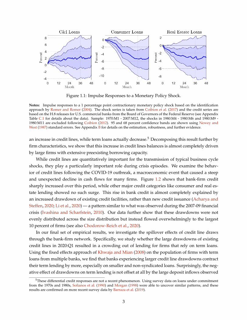
Figure 1.1: Impulse Responses to a Monetary Policy Shock.

Notes: Impulse responses to a 1 percentage point contractionary monetary policy shock based on the identificationapproach by Romer and Romer (2004). The shock series is taken from Coibion et al. (2017) and the credit series arebased on the H.8 releases for U.S. commercial banks from the Board of Governors of the Federal Reserve (see AppendixTable C.1 for details about the data). Sample: 1970:M1 - 2007:M12, the shocks in 1980:M4 - 1980:M6 and 1980:M9 -1980:M11 are excluded following Coibion (2012). 95 and 68 percent confidence bands are shown using Newey andWest (1987) standard errors. See Appendix B for details on the estimation, robustness, and further evidence.

an increase in credit lines, while term loans actually decrease.5 Decomposing this result further byfirm characteristics, we show that this increase in credit lines balances is almost completely drivenby large firms with extensive preexisting borrowing capacity.

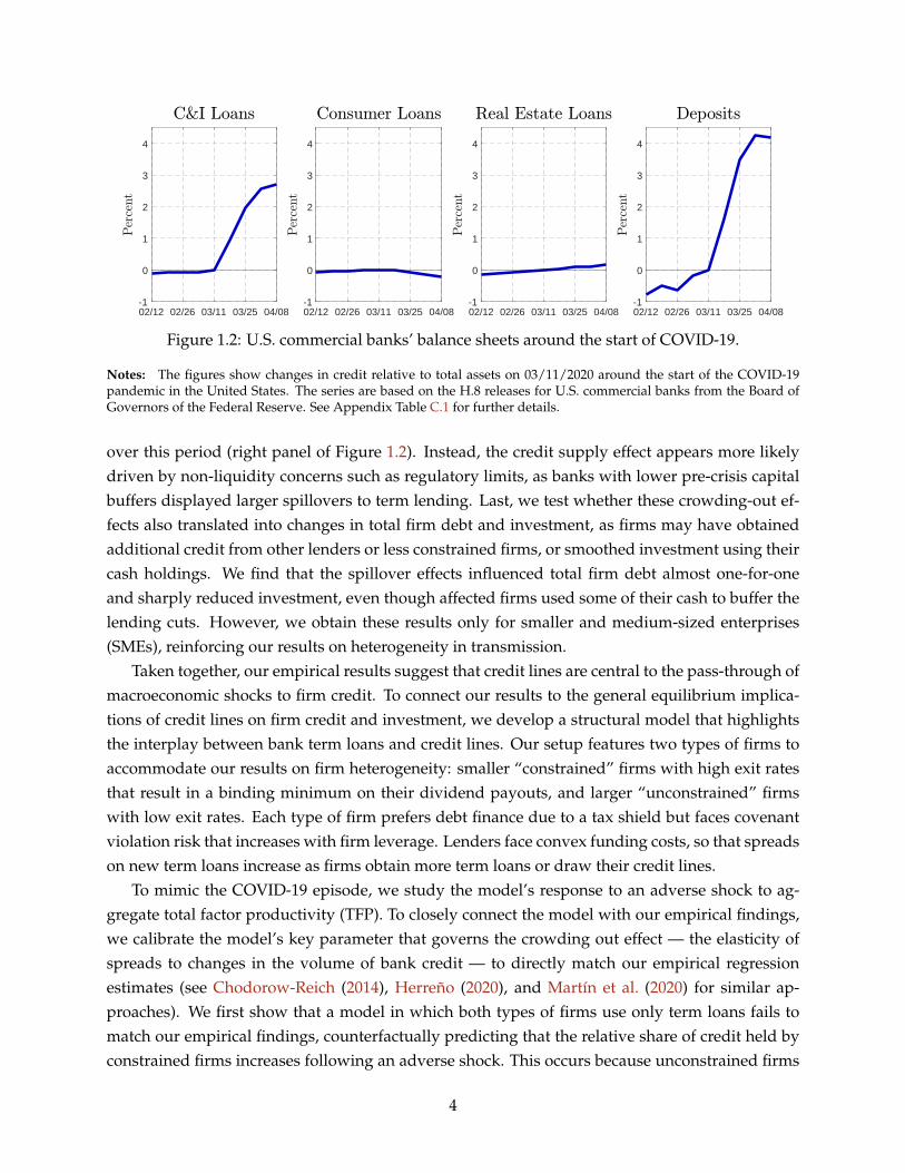
While credit lines are quantitatively important for the transmission of typical business cycleshocks, they play a particularly important role during crisis episodes. We examine the behav-ior of credit lines following the COVID-19 outbreak, a macroeconomic event that caused a steepand unexpected decline in cash flows for many firms. Figure 1.2 shows that bank-firm creditsharply increased over this period, while other major credit categories like consumer and real es-tate lending showed no such surge. This rise in bank credit is almost completely explained byan increased drawdown of existing credit facilities, rather than new credit issuance (Acharya andSteffen, 2020; Li et al., 2020) — a pattern similar to what was observed during the 2007-09 financialcrisis (Ivashina and Scharfstein, 2010). Our data further show that these drawdowns were notevenly distributed across the size distribution but instead flowed overwhelmingly to the largest10 percent of firms (see also Chodorow-Reich et al., 2020).

In our final set of empirical results, we investigate the spillover effects of credit line drawsthrough the bank-firm network. Specifically, we study whether the large drawdowns of existingcredit lines in 2020:Q1 resulted in a crowding out of lending for firms that rely on term loans.Using the fixed effects approach of Khwaja and Mian (2008) on the population of firms with termloans from multiple banks, we find that banks experiencing larger credit line drawdowns contracttheir term lending by more, especially on smaller and non-syndicated loans. Surprisingly, the neg-ative effect of drawdowns on term lending is not offset at all by the large deposit inflows observed

5These differential credit responses are not a recent phenomenon. Using survey data on loans under commitmentfrom the 1970s and 1980s, Sofianos et al. (1990) and Morgan (1998) were able to uncover similar patterns, and theseresults are confirmed on more recent survey data by Barraza et al. (2019).

3

02/12 02/26 03/11 03/25 04/08-1

0

1

2

3

4

02/12 02/26 03/11 03/25 04/08-1

0

1

2

3

4

02/12 02/26 03/11 03/25 04/08-1

0

1

2

3

4

02/12 02/26 03/11 03/25 04/08-1

0

1

2

3

4

Figure 1.2: U.S. commercial banks’ balance sheets around the start of COVID-19.

Notes: The figures show changes in credit relative to total assets on 03/11/2020 around the start of the COVID-19pandemic in the United States. The series are based on the H.8 releases for U.S. commercial banks from the Board ofGovernors of the Federal Reserve. See Appendix Table C.1 for further details.

over this period (right panel of Figure 1.2). Instead, the credit supply effect appears more likelydriven by non-liquidity concerns such as regulatory limits, as banks with lower pre-crisis capitalbuffers displayed larger spillovers to term lending. Last, we test whether these crowding-out ef-fects also translated into changes in total firm debt and investment, as firms may have obtainedadditional credit from other lenders or less constrained firms, or smoothed investment using theircash holdings. We find that the spillover effects influenced total firm debt almost one-for-oneand sharply reduced investment, even though affected firms used some of their cash to buffer thelending cuts. However, we obtain these results only for smaller and medium-sized enterprises(SMEs), reinforcing our results on heterogeneity in transmission.

Taken together, our empirical results suggest that credit lines are central to the pass-through ofmacroeconomic shocks to firm credit. To connect our results to the general equilibrium implica-tions of credit lines on firm credit and investment, we develop a structural model that highlightsthe interplay between bank term loans and credit lines. Our setup features two types of firms toaccommodate our results on firm heterogeneity: smaller “constrained” firms with high exit ratesthat result in a binding minimum on their dividend payouts, and larger “unconstrained” firmswith low exit rates. Each type of firm prefers debt finance due to a tax shield but faces covenantviolation risk that increases with firm leverage. Lenders face convex funding costs, so that spreadson new term loans increase as firms obtain more term loans or draw their credit lines.

To mimic the COVID-19 episode, we study the model’s response to an adverse shock to ag-gregate total factor productivity (TFP). To closely connect the model with our empirical findings,we calibrate the model’s key parameter that governs the crowding out effect — the elasticity ofspreads to changes in the volume of bank credit — to directly match our empirical regressionestimates (see Chodorow-Reich (2014), Herreño (2020), and Martín et al. (2020) for similar ap-proaches). We first show that a model in which both types of firms use only term loans fails tomatch our empirical findings, counterfactually predicting that the relative share of credit held byconstrained firms increases following an adverse shock. This occurs because unconstrained firms

4

have a more elastic demand for credit due to their flexible dividend margin, leading to a relativedecline in their share of credit as spreads rise. Beginning from this baseline, we introduce creditlines, which allow unconstrained firms to borrow at a predetermined, fixed spread. Insulatedfrom rising spreads, these firms borrow heavily, crowding out lending to constrained firms, andreproducing the pattern observed in the data.

In aggregate, the presence of credit lines sharply increases total credit growth to firms follow-ing the negative shock, reproducing the pattern documented in Figure 1.2. This occurs because un-constrained firms, now insulated from deteriorating credit conditions by the ex-ante fixed spreadson credit line facilities, borrow heavily, while constrained firms, in an effort to avoid further costlydisinvestment, do not decrease their borrowing by an offsetting amount, despite high spreads. Butwhile aggregate credit increases, aggregate investment declines more in an economy with creditlines. This occurs due to a large flow of credit away from constrained firms with a high marginalpropensity to invest, and toward unconstrained firms with a low marginal propensity to invest.

Quantitatively, our model implies that the capital stock contracts over the 20Q following theshock more than twice as much in our benchmark economy with credit lines (0.56%) compared toa counterfactual economy without credit lines (0.26%). Instead, much of the additional credit isused to dampen the decline in dividends paid by unconstrained firms, which fall more than seventimes less on impact relative to the counterfactual economy (4.63% vs. 35.70%). We show thatthese same qualitative results carry over in an extension to the model with policy interventions inthe bond market, but are quantitatively muted. Thus, one of the most important impacts of bondmarket interventions over this period may have been indirect, by improving credit access to smallfirms dependent on bank credit.

In summary, our results point to a world in which the corporate sector as a whole has accessto large amounts of credit, even in bad times, but where cross-sectional disparities in access toprecommitted credit have powerful implications for the transmission of macroeconomic shocksinto corporate debt and investment.

Related Literature. Our paper relates to a large literature on the transmission of macroeconomicshocks through credit markets.6 For example, the credit channel of monetary policy posits thatthe “direct effects of monetary policy on interest rates are amplified by endogenous changes inthe external finance premium” (Bernanke and Gertler, 1995). Importantly, an increase in bank-firm credit after a monetary tightening should not be taken as evidence against such a channel.Instead, our main contribution is the finding that amplification mechanisms such as the creditchannel are mitigated for a subset of firms — those with credit lines — and, as a result, are evenstronger for other firms. In this regard, we contribute to a growing literature that emphasizesthe heterogeneous effects of macroeconomic shocks, with several recent contributions focusing on

6See e.g., Bernanke et al. (1999), Kiyotaki and Moore (1997), Gertler and Gilchrist (1993a) Gertler and Gilchrist(1994), among many others, and Lian and Ma (2021) for a recent example.

5

firm responses to changes in monetary policy.7 Our paper complements this work by demonstrat-ing the centrality of credit lines in driving this phenomenon, which has distinct aggregate andcross-sectional consequences for firm credit and investment.

Turning to the corporate finance literature, we relate to an extensive body of work finding thatthe pricing and availability of credit lines depend on the risk exposure of both lenders and borrow-ers.8 In addition, several papers have shown that credit lines are an important source of fundingfor firms in times of distress.9 For example, Brown et al. (2020) use weather events as instrumentsfor cash flow shocks and find that firms use their credit lines to smooth out such shocks. Wefind estimated responses close to theirs, and further show that firms do not smooth using othertypes of bank credit in a significant way. Relative to this literature, we take a more macroeco-nomic perspective that focuses on the aggregate implications of credit lines, made possible by ourcomprehensive administrative data and the general equilibrium model.

We also obtain important context for our work from the literature on covenant violations. Sufi(2009) and Chodorow-Reich and Falato (2021) show that firms can lose access to their credit lineswhen they violate their financial covenants. As a result, our findings on the credit line channelshould be valid in environments where large, unconstrained firms do not violate their covenants,or when banks are unable or unwilling to restrict credit line access to these firms.

We also connect to a large literature that measures the effects of bank health on the allocation offirm credit (e.g., Khwaja and Mian, 2008) and regional or firm outcomes (e.g., Peek and Rosengren,2000; Chodorow-Reich, 2014).10 Our contribution to this literature is to present new evidence thatprecommitted credit lines can drive a quantitatively important shock to bank balance sheets whena large number of firms draw on their existing credit lines simultaneously. We build on Ivashinaand Scharfstein (2010) and Cornett et al. (2011), who provide similar evidence for the 2007-09financial crisis.11 These papers use DealScan and Call Reports data, respectively, to documentthat banks with larger committed credit line exposure cut lending more in the financial crisis.Compared to these works, our matched bank-firm data set allows us to: (i) measure the actualdrawdowns of credit lines at each bank, rather than using exposure to proxy for this variable;(ii) document which firms and loan types are crowded out; (iii) control for endogenous matchingbetween banks and firms using the Khwaja and Mian (2008) borrower fixed effects approach; and(iv) trace out the real effects of crowding out at the firm level. Our cross-sectional regressionestimates further enable us to calibrate a macroeconomic model and derive general equilibrium

7Examples of recent papers are Ottonello and Winberry (2020), Crouzet and Mehrotra (2020), Jeenas (2019), Cloyneet al. (2019), Bahaj et al. (2020), Darmouni et al. (2020), and Anderson and Cesa-Bianchi (2020), among others, whichbuild on the work by Gertler and Gilchrist (1994).

8See, e.g., Campello et al. (2011), Acharya et al. (2013), Acharya et al. (2014), Ippolito et al. (2016), Berg et al. (2017),Acharya et al. (2019), and Acharya et al. (2021a).

9See, e.g., Jiménez et al. (2009), Lins et al. (2010), Campello et al. (2010), Berrospide and Meisenzahl (2015), Berget al. (2016), and Nikolov et al. (2019).

10See e.g., Ashcraft (2005), Gan (2007), Paravisini (2008), Schnabl (2012), Jiménez et al. (2012, 2014), Iyer et al. (2014),Huber (2018), Jiménez et al. (2020), Paravisini et al. (2020), Blattner et al. (2020), and Martín et al. (2020), as well as Luckand Zimmermann (2020), Caglio et al. (2021), and Bidder et al. (2020) who also use the Y14 data.

11See also the debate between Chari et al. (2008) and Cohen-Cole et al. (2008).

6

implications, an approach that we share with Chodorow-Reich (2014), Herreño (2020), and Martínet al. (2020).

In addition to this past research, a number of contemporaneous papers have used the sameY14 dataset to document credit flows during the COVID-19 episode, the closest being a studyby Chodorow-Reich et al. (2020). While our work focuses on the cross-sectional allocation of un-used credit line commitments, arguing that they are plentiful for large firms and scarce for smallfirms, leading to crowding out, Chodorow-Reich et al. (2020) instead focus on the intensive mar-gin, documenting that smaller firms also drew less of what unused credit line capacity they had.They attribute this finding to the shorter maturities typically found on credit lines to SMEs, whichincrease lenders’ discretion and bargaining power — a separate and parallel channel impingingsmaller firms’ credit access over this period.

Building on the same data set, Caglio et al. (2021) document several facts about the composi-tion of credit by firm size and investigate the implications for the transmission of monetary policy,finding evidence of firm risk-taking behavior. Kapan and Minoiu (2021) use syndicated loan datafrom Dealscan to find evidence of crowding out effects similar to those documented in this paper.Finally, Acharya et al. (2021b) show that the liquidity risk posed by credit line drawdowns hasexplanatory power for bank stock returns during the pandemic.

Overview. The rest of the paper proceeds as follows. Section 2 describes the data, while Section3 establishes several key stylized facts. Section 4, provides evidence on the use of credit lines andborrowing capacity in the cross-section of firms and show how firms adjust their credit usage inresponse to cash flow changes. Section 5, revisits the evidence in Figures 1.1 and 1.2, and studiesthe behavior of firm credit in response to a monetary policy shock and to the outbreak of COVID-19. Section 6 presents a macroeconomic model with credit lines. Section 6.6 provides extensionsand robustness. Section 7 concludes.

2 Data

We assemble the data for our empirical analysis from a variety of sources. All loan information onbank-firm relationships and contract terms comes from the FR Y-14Q H.1 collection for commercialloans. The Y14 data consists of information on loan facilities with over $1 million in committedamount, held in the portfolios of bank holding companies (BHCs) subject to the Dodd-Frank ActStress Tests.12 The number of BHCs in the Y14 has varied over time, starting with 18 BHCs atinception in 2011:Q3 and peaking at 38 BHCs in 2016:Q4.13

12A loan facility is a lending program between a bank and a borrower and can include more than one distinct loan,and possibly contain more than one loan type (e.g., credit line or term loan). Banks classify the facility type accordingto the loan type with the majority of total committed amount. Since term loans are typically fully used immediatelyafter their issuance, the majority of unused term loan borrowing capacity is likely accounted for by unused credit lines.We therefore assume throughout that unused term loans represent unused credit lines, or “unused credit” for short.

13The Federal Reserve requires U.S. BHCs, savings and loan companies, and depository institutions with assetsexceeding given thresholds, and also some foreign banking organizations, to comply with the stress test rules. For

7

We restrict the sample to 2012:Q3 - 2020:Q3. The starting point gives a more even distributionof BHCs across quarters and affords a short phase-in period for the structure of the collection andvariables to stabilize. We select facilities to firms that are identified as commercial and industrial,“other loans,” and loans secured by owner-occupied commercial real estate. We drop all loans tofinancial firms and firms in the real estate sector. Appendix C.3 describes these and other samplerestrictions in detail. Our analysis therefore focuses on bank credit to nonfinancial firms and doesnot cover nonbank credit, bank credit extended by non-Y14 banks, or unobserved firms.

The great strength of the data is its rich cross-sectional information and its unparalleled viewinto loan contracting arrangements for a broad spectrum of firms, especially firms that are smallerand non-publicly traded. In particular, we observe not only the committed amount of the facility,but also the amount utilized in each quarter, allowing us to precisely measure a firm’s unusedborrowing capacity. Our primary way of identifying a distinct firm is through the Taxpayer Iden-tification Number (TIN). There are 207,505 distinct TINs observed in the Y14 over the sampleperiod, among which we identify 3,222 public firms that can be matched to Compustat data.

The firm financial statement variables are combined from three sources: Compustat, the Y14,and Orbis. We use financial statement data from the quarterly Compustat files whenever possiblebecause publicly traded firms have accurate and uninterrupted quarterly data for the key variablesof interest. For all other firms we default to the Y14 financials data, which is typically recordedannually. Since firm financial data are reported at the facility level in the Y14 data, we measurefinancial variables for a given firm as the medians of those variables over all facilities held bythat firm. In addition, if a variable is also observed for a private firm in Orbis, we average thevariables from the two sources as a way of further reducing measurement error.14 The Orbis dataalso provides us with a measure of firm age for a wide range of private and public firms, definedas the number of years between the data observation date and the firm incorporation date.15

Our data sources do not include information on lending covenants. To bridge this gap, we useheuristic covenant formulae taken from Dealscan and apply them to the firm financial statementdata (see Appendix C.2 and Section 3 for details). All nominal variables are deflated using theconsumer price index for all items. Variable descriptions, data sources, and a list of cleaning anddata filtering steps can be found in Appendix C.

3 Descriptive Evidence

In this section, we establish several key stylized facts demonstrating the importance of credit linesfor aggregate and cross-sectional credit patterns. We focus on the portion of the sample beforethe start of the outbreak of COVID-19 in the United States (2012:Q3-2019:Q4), and therefore more

most of the sample period, the size threshold was set at $50 billion. In 2019, the threshold was increased to $100 billion.14If the Y14 and Orbis data do not differ by more than 5 percent for a particular firm-date observation, then we

average the variables from the two sources but exclude the observation otherwise.15To supplement our age data, we use the Field-Ritter data set of company founding dates for public firms (Field and

Karpoff, 2002; Loughran and Ritter, 2004), using the Field-Ritter date whenever the value in the Orbis data is missingor the Field-Ritter founding date is older than the one according to Orbis.

8

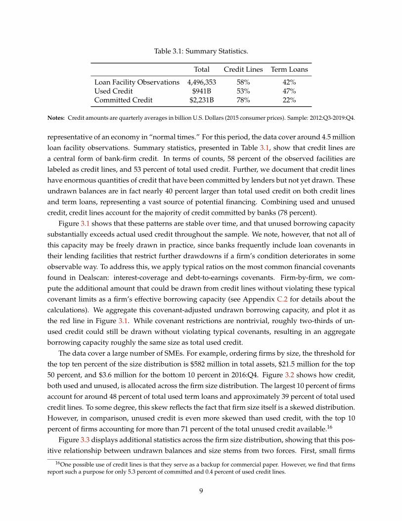
Table 3.1: Summary Statistics.

Total Credit Lines Term Loans

Loan Facility Observations 4,496,353 58% 42%Used Credit $941B 53% 47%Committed Credit $2,231B 78% 22%

Notes: Credit amounts are quarterly averages in billion U.S. Dollars (2015 consumer prices). Sample: 2012:Q3-2019:Q4.

representative of an economy in “normal times.” For this period, the data cover around 4.5 millionloan facility observations. Summary statistics, presented in Table 3.1, show that credit lines area central form of bank-firm credit. In terms of counts, 58 percent of the observed facilities arelabeled as credit lines, and 53 percent of total used credit. Further, we document that credit lineshave enormous quantities of credit that have been committed by lenders but not yet drawn. Theseundrawn balances are in fact nearly 40 percent larger than total used credit on both credit linesand term loans, representing a vast source of potential financing. Combining used and unusedcredit, credit lines account for the majority of credit committed by banks (78 percent).

Figure 3.1 shows that these patterns are stable over time, and that unused borrowing capacitysubstantially exceeds actual used credit throughout the sample. We note, however, that not all ofthis capacity may be freely drawn in practice, since banks frequently include loan covenants intheir lending facilities that restrict further drawdowns if a firm’s condition deteriorates in someobservable way. To address this, we apply typical ratios on the most common financial covenantsfound in Dealscan: interest-coverage and debt-to-earnings covenants. Firm-by-firm, we com-pute the additional amount that could be drawn from credit lines without violating these typicalcovenant limits as a firm’s effective borrowing capacity (see Appendix C.2 for details about thecalculations). We aggregate this covenant-adjusted undrawn borrowing capacity, and plot it asthe red line in Figure 3.1. While covenant restrictions are nontrivial, roughly two-thirds of un-used credit could still be drawn without violating typical covenants, resulting in an aggregateborrowing capacity roughly the same size as total used credit.

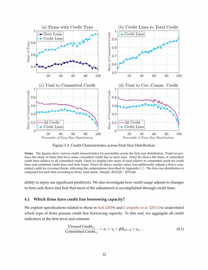
The data cover a large number of SMEs. For example, ordering firms by size, the threshold forthe top ten percent of the size distribution is $582 million in total assets, $21.5 million for the top50 percent, and $3.6 million for the bottom 10 percent in 2016:Q4. Figure 3.2 shows how credit,both used and unused, is allocated across the firm size distribution. The largest 10 percent of firmsaccount for around 48 percent of total used term loans and approximately 39 percent of total usedcredit lines. To some degree, this skew reflects the fact that firm size itself is a skewed distribution.However, in comparison, unused credit is even more skewed than used credit, with the top 10percent of firms accounting for more than 71 percent of the total unused credit available.16

Figure 3.3 displays additional statistics across the firm size distribution, showing that this pos-itive relationship between undrawn balances and size stems from two forces. First, small firms

16One possible use of credit lines is that they serve as a backup for commercial paper. However, we find that firmsreport such a purpose for only 5.3 percent of committed and 0.4 percent of used credit lines.

9

2013Q1 2015Q1 2017Q1 2019Q10

500

1000

1500

2000

2500

3000

Figure 3.1: Aggregate term loans and credit lines.

Notes: The figure shows the total amount of term loans and credit lines across all banks in billion U.S. dollars. Un-used credit is the difference between committed and used credit of credit lines and term loans. The red line indicatescovenant-adjusted undrawn borrowing capacity (see text and Appendix C.2 for details). Sample: 2012:Q3 - 2019:Q4.

have lower committed credit line balances. Panel (a) shows that while nearly 100 percent of thelargest firms have a credit line facility, that share drops close to 60 percent for the smallest firms.Panel (b) shows that the share of credit lines to total committed credit also trends upward withsize.17 Since firms have incentives to draw credit lines in periods of distress, these patterns mayreflect banks’ preference for allocating credit line facilities and balances to larger, more profitablefirms that are further from the distress boundary (Sufi, 2009).

Second, small firms have lower undrawn credit balances because they utilize more of their com-mitted credit. Panel (c) shows that, while firms below the 80th size percentile use a sizable andstable fraction of their committed credit balances, the very largest firms use little of their com-mitted credit line balances, a pattern that is even stronger adjusting for typical covenants (panel(d)). These results point to an additional key reason why small firms lack credit line capacity afteradverse shocks. Faced with a trade-off between reserving committed balances to insure againstshocks and drawing down committed balances today (e.g., for investment), these smaller, finan-cially constrained firms choose to use more credit in normal times. As a result, even when smallfirms have access to credit line facilities, their utilization policy may prevent them from drawingadditional balances following negative shocks.

17Since we observe only borrowing at a subset of banks, a potential concern is that smaller firms may obtain creditlines from banks that fall outside our data. Based on a firm’s total debt from all sources, we are able to verify thatour Y14 bank debt contains the majority of total debt for the smaller firms in our sample (see Appendix Figure D.2).The documented patterns can therefore only change for a larger set of firms if the small firms outside of our data aresubstantially different than the ones that we observe.

10

0 20 40 60 80 1000

0.2

0.4

0.6

0.8

1

Figure 3.2: Cumulative Shares across Firm Size Distribution.

Notes: The figure shows the cumulative shares of used term loans, used credit lines, unused credit, and unused creditadjusted for generic covenant rules (“Cov.”) across the firm size distribution. Unused credit is the difference betweenall committed and used credit, which is additionally adjusted by applying generic covenant rules (see Appendix C.2 fordetails). The firm size distribution is obtained for each date according to firms’ total assets. Sample: 2012:Q3 - 2019:Q4.

Appendix Figures D.1-D.3 further show that larger firms receive lower interest rates, are ratedmore creditworthy according to the banks’ internal ratings, are less likely to post collateral, andpost less collateral relative to the size of the loan when they do. Smaller firms obtain more fixed-rate and nonsyndicated loans, show higher probabilities of default, often use real estate as a formof collateral, and take on longer-maturity term loans but shorter-maturity credit lines (see alsoChodorow-Reich et al., 2020; Caglio et al., 2021).

Last, we investigate credit line pricing. The majority of credit line facilities in the Y14 data arevariable-rate loans with fixed spreads. While spreads can in principle be renegotiated, we findthat the spread on more than 90 percent of credit lines remains completely unchanged throughouttheir history, implying that it is safe to consider these spreads as constant over time.

Taken together, the data offer a detailed view into the composition of bank credit for a muchlarger set of U.S. firms than is typically studied. We show that credit lines account for the majorityof used and committed firm credit held by large banks. Cross-sectionally, credit line access and un-used borrowing capacity are overwhelmingly concentrated among the largest, most creditworthyfirms, and exhibit skewness even beyond what is observed for total credit.

4 Determinants and Use of Firm Credit

In this section, we present results from simple empirical models measuring what determines afirm’s unused borrowing capacity beyond its size. We show that various proxies for a borrower’s

11

20 40 60 80 100

0.4

0.6

0.8

1

20 40 60 80 1000.5

0.6

0.7

0.8

0.9

1

20 40 60 80 1000

0.2

0.4

0.6

0.8

1

20 40 60 80 1000

0.2

0.4

0.6

0.8

1

Figure 3.3: Credit Characteristics across Firm Size Distribution.

Notes: The figures show various credit characteristics for percentiles across the firm size distribution. Panel (a) por-trays the share of firms that have some committed credit line or term loan. Panel (b) shows the share of committedcredit lines relative to all committed credit. Panel (c) displays the share of used relative to committed credit for creditlines and combined credit lines and term loans. Panel (d) shows similar ratios, but additionally adjusts a firm’s com-mitted credit for covenant limits, following the computations described in Appendix C.2. The firm size distribution iscomputed for each date according to firms’ total assets. Sample: 2012:Q3 - 2019:Q4.

ability to repay are significant predictors. We also investigate how credit usage adjusts to changesin firm cash flows and find that most of the adjustment is accomplished through credit lines.

4.1 Which firms have credit line borrowing capacity?

We explore specifications related to those in Sufi (2009) and Campello et al. (2011) to understandwhich type of firms possess credit line borrowing capacity. To this end, we aggregate all creditindicators at the firm level and estimate

Unused Crediti,t

Committed Crediti,t= αt + τk + βXi,t−4 + ui,t , (4.1)

12

Table 4.1: Credit Line Borrowing Capacity.

Size Age Public EBITDA Leverage Tangible Assets Inv. Grade

Coeff. 0.02*** 0.02*** 0.13*** 0.28*** -0.58*** 0.18*** 0.12***(0.00) (0.00) (0.01) (0.01) (0.01) (0.01) (0.00)

R-squared 0.27

Notes: Estimation results for regression (4.1). Standard errors in parentheses are clustered by firm. Sample: 2012:Q3 -2019:Q4. Observations: 156,010. Number of firms: 31,209. ∗∗∗p < 0.01, ∗∗p < 0.05, ∗p < 0.1.

where the dependent variable is the firm’s level of unused borrowing capacity on credit lines (1-used credit/committed credit). All specifications include time (αt) and industry (τk) fixed effects.The vector Xi,t−4 collects several controls that are lagged by four quarters. Firm size is defined asthe natural log of a firm’s noncash assets. EBITDA and tangible assets are scaled by a firm’s non-cash assets, while leverage is defined as total liabilities over total assets.18 Investment Grade andPublic are dummy variables denoting whether a firm has an internal rating of BBB or better, andis publicly traded, respectively. For the estimation, we also adjust firms’ unused and committedbalances for covenants as described above in Section 3.

The results in Table 4.1 show that a higher unused borrowing capacity is more commonly ob-served among large, old, public, and profitable firms with low leverage that possess more tangibleassets and are well rated. These are all well-known proxies for firm credit constraints (see, e.g.,Cloyne et al., 2019). These results are consistent with theoretical models that stress the interplaybetween firm demand for liquidity insurance with lender concerns about moral hazard and otheragency problems (e.g., Holmström and Tirole, 1998; Acharya et al., 2014).

As shown in Appendix Table E.1, we obtain estimated coefficients with largely the same signsfor two alternative dependent variables in regression (4.1): (i) the log-odds ratio of a 0-1 variable,denoting whether a firm has a credit line facility with a positive committed balance, and (ii) acredit line intensity variable (unused credit/(unused credit + cash)) that measures the extent towhich a firm relies on its observed credit line capacity relative to cash as a source of liquidity.Older, public, profitable firms with low leverage are more likely to possess credit line access andtend to rely more heavily on unused credit lines as a potential source of liquidity.19

18To eliminate outliers and data entry errors, we exclude observations within the 1 percent tails of the distributionsfor EBITDA, tangible assets (both relative to noncash assets), and leverage.

19In Appendix E.1, we also compare estimations with and without covenant adjustments (Table E.2) and split thesample into private and public firms for the specification without covenant adjustments (Table E.3). Broadly, specifica-tions without covenant adjustments give similar results. In the private-public firm split, firm profitability is particularlyimportant for explaining whether private firms have credit lines and how much unused capacity they possess.

13

4.2 Credit Responses to Cash Flow Changes

We next investigate how firms use various bank credit instruments to smooth through shocks totheir cash flows. We estimate credit responses using the local projections

Li,t+h−3 − Li,t−4

0.5 (Li,t+h−3 + Li,t−4)= αh

i + τht,k + βh ∆4CFi,t

Assetsi,t−4+ γhXi,t−4 + uh

i,t−3 , (4.2)

where h = 0, 1, 2, ..., 8 and Li,t denotes credit of firm i at time t. In this regression setup, we usethe symmetric growth rate of firm i’s credit as the dependent variable.20 This symmetric growthrate is able to accommodate changes in credit from a starting level of zero, and is always boundedbetween −2 and 2, removing the typical challenge of extreme outliers and the need to winsorize.

We measure growth between t− 4 and t+ h− 3 due to a timing feature of our data. Specifically,our main cash flow variable records total net income over the preceding 12 months. As a result,the 4Q change in this variable at time t reflects changes in the period from t − 3 to t relative tothe period from t− 7 to t− 4. Since the change in cash flows could thus have occurred as earlyas t − 3, we begin our impulse response at that time (h = 0). At the same time, ∆4CFi,t reflectschanges in cash flows as late as time t, we should expect the estimated effects to build betweenh = 0 (time t− 3) and h = 3 (time t) as additional shocks arrive.

Our coefficient of interest is βh, associated with a firm’s change in cash flow ∆4CFi,t scaled bytotal assets. In addition, all specifications include a firm-horizon fixed effect (αh

i ) and an industry-time-horizon fixed effect (τh

t,k). The vector Xi,t−4 contains several firm controls: log of total assets,(cash and marketable securities)/total assets, tangible assets/total assets, and leverage. All firmfinancial variables are lagged by four quarters. In addition, Xi,t−4 includes two lagged values ofthe change in the cash flow variable and two lags of the four-quarter change in the dependentvariable to account for possible serial correlation. Moreover, to address outliers and measurementerror in ∆4CFi,t/Assetsi,t−4, as well as to focus on typical cash flow changes, we exclude absoluteannual changes of ∆4CFi,t/Assetsi,t−4 that are larger than 5 percentage points.21

The various control variables are intended to absorb non-cash flow drivers of firm credit, sothat βh captures the remaining variation due to cash flow changes. Even so, interpreting βh as acausal estimate would face identification challenges. Instead, our results focus on the differencesin βh across credit categories to decompose the roles of credit lines and term loans in driving theobserved correlations of cash flow changes and credit growth at various horizons.

Figure 4.1 shows the negative of the estimated coefficients βh to facilitate the interpretation.After a fall in net income, firms increase their total use of credit immediately (panel (a)). Therise in credit to a negative cash flow change reaches a peak after three quarters, and actually

20The symmetric growth rate is the second-order approximation of the log-difference for growth rates around zeroand has been used in a variety of contexts (see, e.g., Gomez et al., 2020).

21This assumption approximately corresponds to excluding observations below the 15th and above the 85th per-centiles of the sample distribution. In addition, the sample is also constrained to a balanced panel and loan historieswith time gaps are excluded. Our results are robust to considering absolute annual changes in net income relative toassets that are smaller than 10 p.p.

14

0 2 4 6 8

-2

-1

0

1

2

3

0 2 4 6 8

-2

-1

0

1

2

3

0 2 4 6 8

-2

-1

0

1

2

3

Figure 4.1: Credit Responses to a Cash-Flow Change.

Notes: Responses of firms’ total used credit, credit lines, and term loans to a one-unit decrease in net income relative toassets, based on the local projection approach in (4.2). Plots display estimates −βh, corresponding to a decline in cashflows. Observations with absolute annual changes in net income relative to assets larger than 5 percent are excluded.The estimations are based on a balanced panel for each credit type and include 9448 (panel (a)), 6751 (panel (b)), and3913 (panel (c)) observations for each impulse response horizon. 95 and 68 percent confidence bands are shown usingstandard errors that are clustered by firm. Sample: 2012:Q3 - 2019:Q4.

becomes negative after around six quarters, indicating that firms’ creditworthiness deteriorates inthe medium run. Panels (b) and (c) show that the rise in total credit is completely accounted for bythe adjustment in credit lines. By contrast, there is no statistically significant adjustment in termloan usage, with point estimates close to zero at all horizons.

To understand the quantitative importance of these effects, we re-estimate regression (4.2) us-ing the one-year change in total firm debt relative to assets as a dependent variable. We find thata $1 drop in net income is associated with an increase in total debt of around 33 cents, which isstatistically different from zero at the 5 percent level.22 Most important for our analysis, we findthat more than half of this change can be accounted for by credit lines drawn in our data, a lowerbound given that we observe only a subset of banks.

In Appendix E.2, we provide two refinements of these results. First, interacting the firm’scash flow change variable with lagged borrowing capacity shows that the adjustment in creditline usage is strongest for firms that have relatively more capacity prior to the cash flow change(Figure E.1). Second, there is relatively little adjustment in committed credit lines to changes incash flow. Instead, the response of credit is most clearly detected in a change in utilization rates ofexisting credit lines (Figure E.2).

5 Behavior of Firm Credit around Macroeconomic Events

The evidence so far shows that credit lines account for the majority of bank-firm credit in the ag-gregate and enable firms to meet their short-run liquidity needs following changes to their cash

22This estimate is very close to the one by Brown et al. (2020) who use weather events to instrument for cash-flowshocks and find a total debt increase of 35 cents for a $1 drop in net income.

15

flows. In this section, we study the role of credit lines in shaping the response of firm borrow-ing to macroeconomic shocks in the aggregate and the cross-section. In particular, we revisit theevidence presented in the introduction on the responses of bank-firm credit to monetary policyshocks and to the outbreak of COVID-19. We show that credit lines are the main driver of theincrease in overall credit to these two types of adverse macroeconomic shocks.

5.1 Credit Responses to Monetary Policy Surprises

We take two approaches to understand whether the responses in Figure 1.1 can be explained byan increase in credit lines after a monetary policy tightening. First, we construct aggregate timeseries for term loans and credit lines based on the micro-data and estimate separate responses foreach. Second, to study the cross-sectional reallocation induced by these shocks, we replicate theresponses using firm level data in Appendix F.2, which also allows us to decompose the aggregateresponse by prior firm characteristics.

Denote the total loan volume of some credit type at time t across all firms i = 1, ..., N and banksj = 1, ..., J by Lt = ∑N

i=1 ∑Jj=1 Lj

i,t. Based on these quarterly “aggregate” time series, we estimateimpulse responses using the specification

Lt+h − Lt−1

Lt−1= αh + βhεMP

t + γhXt−1 + uht , (5.1)

where h = 0, 1, ..., 8 and εMPt denotes the monetary policy shock at time t. Since the short-term

policy rate was expected to remain at its lower bound for a large part of the sample for which theY14 data is available, we use surprise movements in the two-year government bond yield as ameasure of the shock. In particular, we employ the high-frequency identification approach as inGürkaynak et al. (2005) based on the assumption that monetary policy news dominates over otherfactors in such tight windows.23 To match the frequency of the Y14 data, we convert the surprisesfrom a meeting-by-meeting frequency to a quarterly frequency by summing all meeting surpriseswithin a quarter. The resulting series is shown in Appendix Figure F.1. The vector Xt−1 collectsseveral controls: two lagged values of the one-quarter growth rate of the dependent variable andtwo lags of the monetary policy shock.24

The coefficient of interest in (5.1) is βh, which captures the response of credit at horizon hto a monetary policy shock. For the sample 2012:Q3 - 2019:Q4, Figure 5.1 shows the estimatedcoefficients, depending on whether the credit type are credit lines, term loans, or the sum of thetwo. Reassuringly, the response of all credit (panel (a)) takes a similar shape as that of Figure1.1 for a more recent sample, showing an expansion of aggregate bank-firm credit following a

23The surprises are given by changes in the two-year Treasury note over a 30-minute-window around policy an-nouncements: 10 minutes before, 20 minutes after an announcement.

24The lag length is chosen to yield good performance, as measured by the Aikake and Bayes information criteria,across outcome variables and impulse response horizons. In unreported results, we find that the results are similarwithout any controls or using four lagged values of both the one-quarter growth rate of the dependent variable and themonetary policy shock.

16

0 2 4 6 8

-20

0

20

40

0 2 4 6 8

-20

0

20

40

0 2 4 6 8

-20

0

20

40

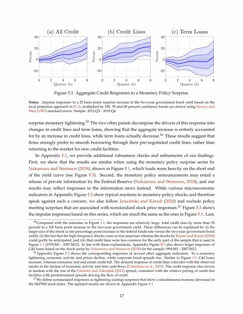
Figure 5.1: Aggregate Credit Responses to a Monetary Policy Surprise.

Notes: Impulse responses to a 25 basis point surprise increase in the two-year government bond yield based on thelocal projection approach in (5.1), multiplied by 100. 95 and 68 percent confidence bands are shown using Newey andWest (1987) standard errors. Sample: 2012:Q3 - 2019:Q4.

surprise monetary tightening.25 The two other panels decompose the drivers of this response intochanges in credit lines and term loans, showing that the aggregate increase is entirely accountedfor by an increase in credit lines, while term loans actually decrease.26 These results suggest thatfirms strongly prefer to smooth borrowing through their pre-negotiated credit lines, rather thanreturning to the market for new credit facilities.

In Appendix F.1, we provide additional robustness checks and refinements of our findings.First, we show that the results are similar when using the monetary policy surprise series byNakamura and Steinsson (2018), shown in Figure F.1, which loads more heavily on the short endof the yield curve (see Figure F.3). Second, the monetary policy announcements may entail arelease of private information by the Federal Reserve (Nakamura and Steinsson, 2018), and ourresults may reflect responses to the information news instead. While various macroeconomicindicators in Appendix Figure F.2 show typical reactions to monetary policy shocks and thereforespeak against such a concern, we also follow Jarocinski and Karadi (2020) and exclude policymeeting surprises that are associated with nonstandard stock price responses.27 Figure F.3 showsthe impulse responses based on this series, which are much the same as the ones in Figure 5.1. Last,

25Compared with the estimates in Figure 1.1, the responses are relatively large: total credit rises by more than 50percent to a 100 basis point increase in the two-year government yield. These differences can be explained by (i) thelarger size of the shock (a one percentage point increase in the federal funds rate versus the two-year government bondyield), (ii) the fact that the high-frequency shocks come as true surprises whereas the shocks by Romer and Romer (2004)could partly be anticipated, and (iii) that credit lines were less common for the early part of the sample that is used inFigure 1.1 (1970:M1 - 2007:M12). In line with these explanations, Appendix Figure B.3 also shows larger responses ofC&I loans based on the shock series by Nakamura and Steinsson (2018) for the sample 1994:M1 - 2007:M12.

26Appendix Figure F.2 shows the corresponding responses of several other aggregate indicators. To a monetarytightening, economic activity and prices decline, while corporate bond spreads rise. Similar to Figure 1.1, C&I loansincrease, whereas consumer and real estate credit fall. The delayed response of credit lines coincides with the observedinertia in the decline of economic activity and firm cash-flows (Christiano et al., 2005). The credit response also movesin tandem with the rise of the Gilchrist and Zakrajšek (2012) spread, consistent with the relative pricing of credit linefacilities with predetermined spreads driving the flow of credit.

27We define nonstandard responses as tightening (easing) surprises that show a simultaneous increase (decrease) inthe S&P500 stock index. The updated results are shown in Appendix Figure F.1.

17

we use the full scope of the micro-data in Appendix F.2 to understand which firms account for theaggregate responses. We find that the total response of credit lines is almost entirely explainedby firms that are large and have substantial ex-ante borrowing capacity. Taken together, theseresults show that credit lines are quantitatively important for the transmission of monetary policythrough bank lending.

5.2 Credit Movements during the COVID-19 Pandemic

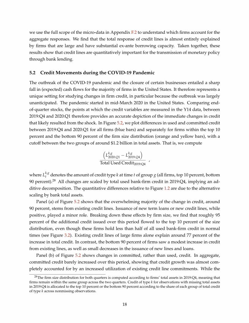
The outbreak of the COVID-19 pandemic and the closure of certain businesses entailed a sharpfall in (expected) cash flows for the majority of firms in the United States. It therefore represents aunique setting for studying changes in firm credit, in particular because the outbreak was largelyunanticipated. The pandemic started in mid-March 2020 in the United States. Comparing end-of-quarter stocks, the points at which the credit variables are measured in the Y14 data, between2019:Q4 and 2020:Q1 therefore provides an accurate depiction of the immediate changes in creditthat likely resulted from the shock. In Figure 5.2, we plot differences in used and committed creditbetween 2019:Q4 and 2020:Q1 for all firms (blue bars) and separately for firms within the top 10percent and the bottom 90 percent of the firm size distribution (orange and yellow bars), with acutoff between the two groups of around $1.2 billion in total assets. That is, we compute(

Lk,g2020:Q1 − Lk,g

2019:Q4

)Total Used Credit2019:Q4

,

where Lk,gt denotes the amount of credit type k at time t of group g (all firms, top 10 percent, bottom

90 percent).28 All changes are scaled by total used bank-firm credit in 2019:Q4, implying an ad-ditive decomposition. The quantitative differences relative to Figure 1.2 are due to the alternativescaling by bank total assets.

Panel (a) of Figure 5.2 shows that the overwhelming majority of the change in credit, around90 percent, stems from existing credit lines. Issuance of new term loans or new credit lines, whilepositive, played a minor role. Breaking down these effects by firm size, we find that roughly 95percent of the additional credit issued over this period flowed to the top 10 percent of the sizedistribution, even though these firms hold less than half of all used bank-firm credit in normaltimes (see Figure 3.2). Existing credit lines of large firms alone explain around 77 percent of theincrease in total credit. In contrast, the bottom 90 percent of firms saw a modest increase in creditfrom existing lines, as well as small decreases in the issuance of new lines and loans.

Panel (b) of Figure 5.2 shows changes in committed, rather than used, credit. In aggregate,committed credit barely increased over this period, showing that credit growth was almost com-pletely accounted for by an increased utilization of existing credit line commitments. While the

28The firm size distribution for both quarters is computed according to firms’ total assets in 2019:Q4, meaning thatfirms remain within the same group across the two quarters. Credit of type k for observations with missing total assetsin 2019:Q4 is allocated to the top 10 percent or the bottom 90 percent according to the share of each group of total creditof type k across nonmissing observations.

18

All Credit

Existing Credit

New Credit Lines

New Term Loans

0

5

10

15

20

25

All Credit

Existing Credit

New Credit Lines

New Term Loans

0

5

10

15

20

25

Figure 5.2: Changes in Used and Committed Credit for 2019:Q4 - 2020:Q1.

Notes: The blue bars show aggregate changes in used and committed credit across all banks between 2019:Q4 and2020:Q1, relative to total used credit in 2019:Q4. The orange and yellow bars display equivalent changes for the 10percent and the bottom 90 percent of the firm size distribution, also relative to total used credit in 2019:Q4. The changesare further separated into differences in existing credit, new credit line issuances, and new term loans (all in percentrelative to all used credit in 2019:Q4). The firm size distribution is computed according to firms’ total assets in 2019:Q4.

largest 10 percent of firms were able to slightly increase the balances of committed credit, thebottom 90 percent displayed a small drop stemming from lower commitments on new facilities.

Appendix Figure F.7 repeats these calculations for changes from 2019:Q4 to 2020:Q2 and to2020:Q3. While more than half of the initial increase of used existing credit tapers off in 2020:Q2,the change for the bottom 90 percent of firms actually turns negative for the two-quarter com-parison and the one for the top 10 percent remains elevated. Similar heterogeneity is present fornew credit issuances. By the end of 2020:Q3, the initial increase in bank-firm credit reversed in theaggregate, with some of the distributional differences still remaining.29

5.3 Credit Supply during the COVID-19 Pandemic

While these patterns indicate that access to credit differed in the cross-section of firms, they donot distinguish between credit demand and supply, and possible spillovers between firms. Inparticular, the large withdrawal of existing credit lines may have put pressure on bank balancesheets. In turn, banks may have reduced their supply of term loans, an important source of creditto SMEs. We test for such crowding out effects by employing a fixed effect regression similar toKhwaja and Mian (2008). The methodology for estimating a credit supply channel focuses on

29In Appendix F.3, we provide further evidence that credit shifted toward less financially constrained firms. Firmsthat accessed their credit lines in 2020:Q1 were disproportionately large, profitable, and public firms compared to the2012:Q3 - 2019:Q4 presample (see also Chodorow-Reich et al., 2020).

19

firms borrowing from multiple banks, where banks differ in their exposure to the outbreak ofCOVID-19. As a measure of exposure, we use variation in drawdowns on existing credit lines.

The approach relies on two key identifying assumptions. First, the shock must be exogenous,an assumption that we believe is satisfied, since the outbreak was largely unanticipated at theend of 2019. Second, a firm’s demand for term loans should not depend on its bank’s differentialexposure to the shock, holding the terms of the loan fixed. This second assumption would, forexample, be violated if firms substitute between credit lines and term loans at some bank. Onepossible reason for such a relation is that credit lines become relatively cheaper when the generalcost of credit increases, since they feature fixed, predetermined spreads. To ensure that the secondidentifying assumption is satisfied, we restrict the sample to term loans only, and exclude caseswhere firms have both term loans and credit lines at the same bank, so that our results are notdriven by substitution between the two. Based on the restricted data set, we estimate

Lj,ki,t+h − Lj,k

i,t−1

0.5(

Lj,ki,t+h + Lj,k

i,t−1

) = αki,h + βh ∆Credit Line Usagej

t

Assetsjt−1

+ µh ∆Depositsjt

Assetsjt−1

+ γh X jt−1 + uj,k

i,h , (5.2)

for h = 0, 1, 2, where t − 1 denotes 2019:Q4 and t + h is given by one of the following threequarters. For the dependent variable, we use the same formulation as in Section 4.2, which allowsfor possible zero-observations in t − 1 or t + h and is bounded in the range [−2, 2]. Lj,k

i,t is theaggregated loan amount of type k between bank j and firm i at time t. We consider variable- andfixed-rate loans as separate types k to account for possible differences in the demand for such loansdue to changes in short-term interest rates between t− 1 and t + h that may be correlated with thedrawdowns at the bank-level, and we again exclude observations with both types at the samebank. The firm-specific fixed effect αk

i,h absorbs a firm’s common demand for credit type k. Theestimated coefficient β associated with the change of used existing credit lines between t− 1 and tat bank j, relative to total bank assets in t− 1, therefore captures credit supply effects: banks maydiffer in their supply of term loans due to their differential intensity of credit line withdrawals.30

X jt−1 represents a vector of controls, which are omitted in the baseline specification and added

subsequently to test the robustness of the results.The estimation results are shown in Table 5.1. Column (i) shows the results for used term

loans between 2019:Q4 and 2020:Q1. The negative sign of the coefficient β implies that a bankthat experiences a larger drawdown of credit lines restricts its supply of term loans by more andthis effect is statistically different from zero at the 5 percent level.31 In column (ii), we extend the

30Drawdowns on precommitted credit lines cannot generally be refused by banks, unless the borrower has violatedits debt covenants or "material adverse change clauses" (Demiroglu and James, 2011). However, banks may use informalbargaining power to pressure firms not to draw their credit lines (Chodorow-Reich et al., 2020) or react to covenantviolations on other credit lines more strongly when they experience large drawdowns (Chodorow-Reich and Falato,2021). If banks discourage drawdowns more when their own balance sheets are impaired, then the estimated effects inTable 5.1 can be seen as a lower bound on the strength of the crowding out effect.

31Alongside these quantity responses, we test for price responses using the change in the interest rate, weighted byused term loans, as a dependent variable in (5.2), and report the results in Appendix Table F.2. For 2020:Q2/Q3, wefind a positive and statistically significant coefficient β. However, these results are sensitive to excluding outliers, andgenerally less precise than our quantity responses.

20

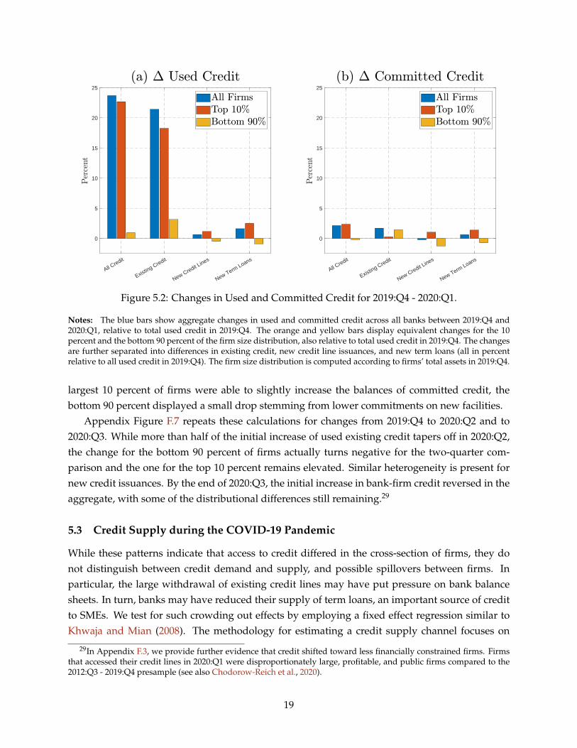
Table 5.1: COVID-19 − Credit Supply.

(i) (ii) (iii) (iv) (v) (vi)2020:Q1 2020:Q1 2020:Q1 2020:Q2 2020:Q3 2020:Q1

∆ Credit Line Usage -1.96** -2.28*** -2.57*** -3.03** -3.63** -1.70**(0.72) (0.65) (0.91) (1.14) (1.62) (0.66)

∆ Deposits 0.14(0.20)

Fixed Effects∗∗ Firm × Rate 3 3 3 3

∗∗ Firm × Rate ×Maturity 3

∗∗ Firm × Rate × Purpose 3

Bank Controls 3 3

R-squared 0.51 0.51 0.55 0.51 0.53 0.51Observations 1,678 1,596 1,007 1,519 1,390 1,638Number of Firms 749 712 464 682 624 733Number of Banks 28 28 27 28 28 26

Notes: Estimation results for regressions (5.2), where the dependent variable is given by changes in credit between2019:Q4 and 2020:Q1 in columns (i)-(iii) and (vi), from 2019:Q4 to 2020:Q2 in column (iv), and between 2019:Q4 and2020:Q3 in column (v). The regressors “∆ Credit Line Usage” and “∆ Deposits” denote the change of a bank’s usedexisting credit lines or deposits from 2019:Q4 to 2020:Q1, relative to total assets in 2019:Q4. All regressions include firm-specific fixed effects that additionally vary by rate type (adjustable- or fixed-rate) and the remaining maturity (columnii) or the loan purpose (column iii). Maturity fixed effects take the form of three bins according to their remainingmaturity in 2019:Q4: (i) less than one quarter, (ii) less than one year, and (iii) more than one year. Columns (iii) and(vi) include various bank controls for 2019:Q4: bank size (natural log of total assets), return on assets (net income/totalassets), leverage (total liabilities/total assets), deposit share (total deposits/total assets), and banks’ income gap (seeAppendix Table C.5 for details on the data). All specifications are estimated using OLS. Standard errors in parenthesesare clustered by bank. Sample: 2019:Q4 - 2020:Q3. ∗∗∗p < 0.01, ∗∗p < 0.05, ∗p < 0.1.

fixed effect to cover not only loan types according to the flexibility of their interest rate but alsoby their remaining maturity. This extension checks the robustness of the results for the possibilitythat the amount of credit line drawdowns and the maturity profile of a bank’s term loan portfolioare correlated, and a firm’s credit demand depends on the remaining maturity (see also Khwajaand Mian, 2008). If anything, the results become stronger with the extended fixed effect.

Another potential identification concern may be that banks specialize in certain types of lend-ing and the associated credit demand for such borrowing is correlated with the credit line draw-downs across banks (Paravisini et al., 2020). For bank specialization to explain our results, bankswould have to hedge their lending activities across loan types, such that banks with larger creditline drawdowns specialize in providing term loans that are less likely to be associated with firms’short-run liquidity needs. To address this concern, we additionally allow for the firm fixed effectin regression (5.2) to vary with the loan purpose that firms report.32 To account for other pre-crisis

32We distinguish between the purposes "Working Capital," "Capital Expenditures" (including real estate), "M&AFinancing," and "All Other Purposes" (see also Appendix Table C.2).

21

differences across banks, we also include various bank-specific controls that are collected in thevector X j

t−1 in regression (5.2). Among these, bank size could account for the possibility that firmsmay prefer to borrow from smaller relationship banks that offer fewer credit lines during a crisis.Column (iii) in Table 5.1 shows that the results actually intensify with the extended fixed effectand the additional control variables.

In Appendix F.3, we show that these findings are robust to various modifications of the re-gression specification. We first test whether our results hold in the absence of the firm fixed effectαk

i,h. Table F.3 presents these results for the multi-lender subsample, showing that the resultingcoefficients are close to those in Table 5.1. Table F.4 removes the restriction that firms borrow frommultiple lenders, estimating coefficients that are slightly attenuated but highly statistically signif-icant for this extended sample of nearly 30,000 firms. Table F.4 further shows strong spilloversfor firms with a single lender, a subsample that includes many of the smallest firms that we ob-serve. These results illustrate that firm credit demand and bank credit supply shocks are relativelyuncorrelated for that sample of firms, and that the firm fixed effect is not critical to our results.

The crowding out effects that we uncover are potentially a smaller concern if they are rela-tively short-lived. To test for the persistence of the results, we consider changes in the dependentvariable from 2019:Q4 to 2020:Q2/Q3 in regressions (5.2). As shown in columns (iv) and (v) ofTable 5.1, the effects not only remain but actually intensify towards the end of 2020:Q3, eventhough the initial drawdowns were largely repaid by 2020:Q3. Our results are therefore consistentwith inertia or planning time in bank lending decisions, or persistence in the uncertainty of addi-tional drawdowns. Tables F.5 and F.6 compare alternative fixed effect and control specificationsfor 2020:Q2/Q3, showing that the results are robust across these quarters as well.

To measure economic significance, we combine our results using a back-of-the-envelope cal-culation. Given the average ratio of term lending to bank assets that we observe, these estimatesimply a term lending cut of around 10-30 cents for a $1 drawdown of credit lines.33 While thesespillover effects are already substantial, we consider them a lower bound on the total crowdingout effect, which likely extends to other forms of credit not present in our sample such as smallbusiness, consumer, and real estate credit.

Finally, we test how these spillover effects differ by loan characteristics, with the results shownin Appendix Table F.7. Our findings are largely explained by a supply contraction of smaller,fixed-rate, and non-syndicated loans. All of these characteristics are more prevalent among SMEs,implying that these smaller firms faced a sharper lending cut due to drawdowns.

Liquidity and Bank Constraints. These spillover effects are perhaps surprising given that ag-gregate bank deposits increased by more than C&I loans over this period (see Figure 1.2) and, aspointed out in Gatev and Strahan (2006), banks generally have an incentive to match the cyclical-ity of their deposit flows and credit line draws. Even if banks were short on deposits, they could

33This is computed by multiplying the typical ratio of term lending to bank assets across the Y14 banks (∼5 percent)with the range of estimates for β in Tables 5.1, F.5, and F.6, which lie between −2 and −6.

22

have obtained additional liquidity through the interbank market. Taken together, this suggeststhat banks should have had more than sufficient funding to cover their credit line draws withoutcontracting their other lending activity. Instead, we find strong evidence of a credit crunch in themarket for term loans depending on banks’ credit line exposure, a result that we should not obtainif the balance sheet pressures were offset by the available liquidity.

To isolate the role of deposits, we modify the baseline specification and additionally control forthe deposit inflow in the first quarter of 2020, denoted by ∆Depositsj

t/Assetsjt−1 in regressions (5.2),

as well as various other bank characteristics collected in X jt−1.34 Column (vi) in Table 5.1 shows

the estimation results. Despite the additional controls, the estimated coefficient β remains nearlyunchanged compared with the baseline in column (i). At the same time, we find a coefficient closeto zero on the change in deposits, and can easily reject the hypothesis β + µ = 0. In other words,our estimates imply that the combination of a $1 deposit inflow, paired with a simultaneous $1outflow on a drawn credit line is not neutral, but instead causes a significant decrease in thatbank’s supply of term loans. This lack of equivalence between deposit inflows and credit lineoutflows can explain our findings of a term loan crunch in an environment of plentiful deposits.

Aware of the pressure on banks’ balance sheets, policymakers provided liquidity to financialmarkets, established lending programs targeting in particular SMEs, eased restrictions on banks,and also indirectly supported them through various monetary and fiscal actions.35 While ourfindings can be understood as a rationale for such interventions, they also show that the policyactions did not completely offset the pressure from the drawdowns on bank balance sheets, whichwould have instead led us to find β ≈ 0.

We interpret these results as providing strong evidence that banks were averse to taking onadditional risk or were facing constraints on lending in spite of the direct availability of funds inthe weeks following the outbreak of the pandemic. A particular mechanism that can explain ourfindings works through bank regulatory capital. Undrawn balances on credit lines typically have

34The regressors of interest in equation (5.2) show substantial variation across banks. The drawdown on existingcredit lines relative to lagged assets ranges from −0.2 to around 3.6 percent with a standard deviation of around 1percent. The change in deposits relative to lagged assets ranges from 0.9 percent to around 31 percent with a standarddeviation of around 6.7 percent. The two variables are negatively correlated with a correlation coefficient of −0.16,suggesting that a mechanism by which credit line drawdowns are immediately re-deposited at the same bank was nota dominant driver of deposit flows. In addition, using weekly deposit rate data from Ratewatch and weekly balancesheet data for U.S. commercial banks from the FR-2644 forms, we find no evidence that banks that paid higher depositrates attracted more deposits over the period that is shown in Figure 1.2 from 2/12/2020 to 4/8/2020 (results notreported), suggesting that the deposit inflow was not strongly influenced by individual bank policies.

35In response to the outbreak of the pandemic, the Economic Injury Disaster Loans, the Paycheck Protection Program(PPP), and the Main Street Lending Program (MSLP) provided credit to SMEs. With respect to our results, we note thatPPP are not part of the Y14 data, and that while MSLP loans do appear in the Y14 data, our subsample used for ourresults in Table 5.1 does not contain any, likely due to the relatively low initial usage of this program. We believethese lending programs are unlikely to confound our results for three reasons. First, both programs begin in 2020:Q2,while our results are already visible in 2020:Q1. Second, the larger banks that experienced a higher rate of credit linedrawdowns in our data also extended fewer PPP loans on average (Granja et al., 2020). As a result, it is unlikely thatthese banks reduced term lending to our subsample of firms due to substitution into PPP loans. Third, we show inTable 5.2 that our results carry through to total firm debt from all sources, implying that incorporating PPP lendingwould not materially change our findings.

23

substantially lower regulatory risk-weights than drawn balances (Pelzl and Valderrama, 2019).36

When credit lines are used and appear on bank balance sheets, they may therefore tie up bankcapital, leading banks to compensate by cutting their term lending supply. To test whether regu-latory constraints can explain our results, we consider alternative specifications of regression (5.2)that allow for interactions between the credit line drawdowns and bank capital buffers in 2019:Q4.The results are reported in Appendix Table F.8. Consistent with the described mechanism, we findthat banks with lower pre-crisis capital buffers restricted their term lending supply to a greaterdegree in response to drawdowns on their credit lines.

A potential alternative explanation for our results is that banks with larger credit line draw-downs also experienced a stronger decline in the expected profitability of their legacy loans. Inprinciple, declining health could both induce large drawdowns as firms “run” on their credit lines,and also lead the bank to reduce term lending, without any causal link between the two. To ad-dress this concern, we follow two approaches. First, we use an instrumental variable estimationfor regression (5.2). As an instrument for the credit line drawdowns, we use banks’ ratio of un-used credit commitments relative to assets in 2019:Q4 with the identifying assumption that bankswith different ratios have otherwise similar loan portfolios.37 Second, we directly control for thechange in the quality of a bank’s existing term loan portfolio using banks’ reported probabilitiesof default and provision for loan losses from banks’ income statements. The results are reportedin Appendix Table F.9 and are close to our baseline estimates.

Crowding Out Effects on Total Debt and Investment. Our estimates so far reflect relative re-sponses of credit at banks in our sample. Thus, to the extent that firms may substitute acrossbanks, toward non-bank lenders, or receive credit from other firms, the effects of drawdowns ontotal firm debt could differ. The ultimate impact on investment is similarly unclear if firms useother margins, like cash holdings, to replace declines in credit. To address these concerns, we nowturn to the firm financial data, which measures total firm borrowing from all sources, as well asinvestment. Using these data, we estimate firm level regressions of the form

Di,t+1 − Di,t−1

0.5 (Di,t+1 + Di,t−1)= αm + β

J

∑j=1

ωji,t−1

(∆Credit Line Usagej

t

Assetsjt−1

)+ γ Xi,t−1 + ui,t+1 , (5.3)

where Di,t denotes total debt of firm i at time t and αm is an industry fixed effect. The coefficientof interest is β related to the weighted sum of firms’ exposure across all banks in our data. Theassociated interaction terms consist of the observed share of term borrowing to total debt ω

ji,t =

(Term Loanji,t)/Di,t between firm i and bank j and bank j’s exposure to credit line drawdowns that

36Under the Basel framework’s standardized approach to calculating risk-based capital requirements, off-balance-sheet commitments are assigned credit conversion factors (CCFs) depending on maturity. Exposures with originalmaturity under one year receive a CCF of 20 percent, while exposures with maturities over one year receive a 50percent CCF. If the commitment can be unconditionally canceled at any time, the exposure receives a zero percent CCF,or a zero-risk weighting.

37Bank credit line drawdowns in 2020:Q1 and their unused commitments before the outbreak of the pandemic arestrongly positively correlated with a correlation coefficient of 0.67, showing that much of banks’ differential exposurein regressions (5.2) originates from differences in prior commitments.

24

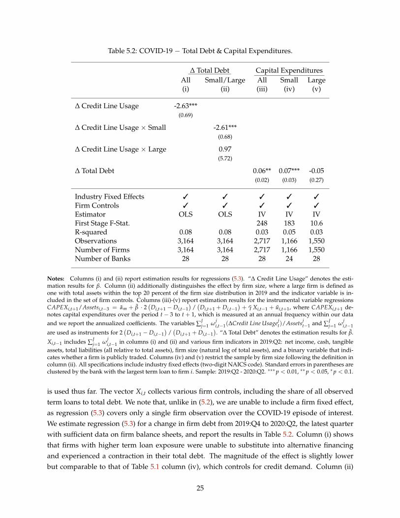
Table 5.2: COVID-19 − Total Debt & Capital Expenditures.

∆ Total Debt Capital ExpendituresAll Small/Large All Small Large(i) (ii) (iii) (iv) (v)

∆ Credit Line Usage -2.63***(0.69)

∆ Credit Line Usage × Small -2.61***(0.68)

∆ Credit Line Usage × Large 0.97(5.72)

∆ Total Debt 0.06** 0.07*** -0.05(0.02) (0.03) (0.27)

Industry Fixed Effects 3 3 3 3 3

Firm Controls 3 3 3 3 3

Estimator OLS OLS IV IV IVFirst Stage F-Stat. 248 183 10.6R-squared 0.08 0.08 0.03 0.05 0.03Observations 3,164 3,164 2,717 1,166 1,550Number of Firms 3,164 3,164 2,717 1,166 1,550Number of Banks 28 28 28 24 28

Notes: Columns (i) and (ii) report estimation results for regressions (5.3). “∆ Credit Line Usage” denotes the esti-mation results for β. Column (ii) additionally distinguishes the effect by firm size, where a large firm is defined asone with total assets within the top 20 percent of the firm size distribution in 2019 and the indicator variable is in-cluded in the set of firm controls. Columns (iii)-(v) report estimation results for the instrumental variable regressionsCAPEXi,t+1/Assetsi,t−3 = αm + β · 2

(Di,t+1 − Di,t−1

)/(

Di,t+1 + Di,t−1)+ γ Xi,t−1 + ui,t+1, where CAPEXi,t+1 de-

notes capital expenditures over the period t − 3 to t + 1, which is measured at an annual frequency within our dataand we report the annualized coefficients. The variables ∑J

j=1 ωji,t−1(∆Credit Line Usagej

t)/Assetsjt−1 and ∑J

j=1 ωji,t−1

are used as instruments for 2(

Di,t+1 − Di,t−1)

/(

Di,t+1 + Di,t−1). “∆ Total Debt” denotes the estimation results for β.

Xi,t−1 includes ∑Jj=1 ω

ji,t−1 in columns (i) and (ii) and various firm indicators in 2019:Q2: net income, cash, tangible

assets, total liabilities (all relative to total assets), firm size (natural log of total assets), and a binary variable that indi-cates whether a firm is publicly traded. Columns (iv) and (v) restrict the sample by firm size following the definition incolumn (ii). All specifications include industry fixed effects (two-digit NAICS code). Standard errors in parentheses areclustered by the bank with the largest term loan to firm i. Sample: 2019:Q2 - 2020:Q2. ∗∗∗p < 0.01, ∗∗p < 0.05, ∗p < 0.1.

is used thus far. The vector Xi,t collects various firm controls, including the share of all observedterm loans to total debt. We note that, unlike in (5.2), we are unable to include a firm fixed effect,as regression (5.3) covers only a single firm observation over the COVID-19 episode of interest.We estimate regression (5.3) for a change in firm debt from 2019:Q4 to 2020:Q2, the latest quarterwith sufficient data on firm balance sheets, and report the results in Table 5.2. Column (i) showsthat firms with higher term loan exposure were unable to substitute into alternative financingand experienced a contraction in their total debt. The magnitude of the effect is slightly lowerbut comparable to that of Table 5.1 column (iv), which controls for credit demand. Column (ii)

25

in Table 5.2 interacts firm term borrowing exposure with measures of firm size, showing that theestimated effects are strongest among SMEs.

In a second step, we employ an instrumental variable regression to investigate whether the re-ductions in firm debt also affected firm investment decisions. The first stage is given by regression(5.3), where firms’ term loan exposure serves as an instrument to estimate the relation betweenfirm debt and capital expenditures in the second stage. Columns (iii)-(v) in Table 5.2 report theresults for all firms, and separately for small and large ones. The positive coefficient in column (iii)shows that reductions in total debt resulted in lower capital expenditures. The relation is againdriven by smaller firms (column (iv)). In contrast, the estimated coefficient is not statistically dif-ferent from zero for large firms (column (v)), in part because of the weak link between term loanexposure and total debt in the first stage. The effects are also economically sizable. The estimatedcoefficient in column (iv) implies a reduction in capital expenditures of around 23 cents for every$1 decline in firm debt, given the typical debt-to-asset ratio in the data.

These results show that firms were unwilling or unable to buffer the lending cuts by using theircash holdings or other resources, leading to a fall in firm investment. To isolate the response offirm cash holdings, we rerun the IV-regressions using the change in cash holdings as a dependentvariable. The results, reported in Appendix Table F.10, show that SMEs partly reacted to the lend-ing cuts by reducing their cash buffers. Without these adjustments, the fall in investment wouldhave likely been even stronger. Taken together, our results show that the credit line drawdownsof large firms following the outbreak of COVID-19 crowded out term lending to SMEs, which inturn resulted in a decline of their total debt and investment.

6 Model

In this section we derive a theoretical model to study the general equilibrium implications of thecredit line channel for firm borrowing and investment. We briefly summarize the key ingredientsof the model, present the detailed structure, calibrate the model, and describe our findings.

6.1 Model Overview

Our model is designed to capture the main empirical patterns we document in Sections 3 - 5. Toaccount for heterogeneity in credit line access in a tractable way, we allow for two types of firms:constrained firms that face a binding lower limit on their dividend payouts, and unconstrainedfirms that do not. Inspired by our empirical findings, the unconstrained firms borrow using creditlines, while the constrained firms borrow using term loans. Importantly, neither type of firm isliterally credit constrained, and both types are able to obtain additional debt at the margin. Instead,all firms find an interior solution for debt that balances the benefits of debt against the increasedcovenant violation risk that comes with higher leverage. As a result, constrained primarily differfrom unconstrained firms in that they use their debt margin exclusively to fund new investments,while unconstrained firms use debt to both invest and pay dividends at the margin.

26

To introduce credit lines in a parsimonious manner, we make the simple assumption that termloans are priced at the market-clearing rate, while credit lines always have a fixed, predeterminedspread over the risk-free interest rate. Lenders face convex funding costs for providing either formof credit, implying that spreads increase with the quantity of credit demanded. As a result, bor-rowing by one type of firm (i.e., unconstrained firms drawing on credit lines) can crowd out creditsupply for the other firms in the economy. Superficially, this assumption is at odds with our find-ings in Tables 5.1 and F.8 showing that spillovers are more consistent with constraints on capitalrequirements than on the direct need to obtain funds. However, we view this convex funding costas a parsimonious approximation of a richer model in which banks face capital constraints butface convex costs of raising capital, where the degree of frictions on equity issuance in this richermodel should map directly into the curvature of our model’s convex funding cost.

To discipline debt accumulation, we impose debt-to-EBITDA covenants that are costly to vio-late following Greenwald (2019). Firms face idiosyncratic risk, leading them to reduce their prob-ability of violation by keeping a precautionary buffer between their debt-to-EBITDA ratio and thecovenant threshold. This specification matches the findings by Sufi (2009) that firms with creditlines are typically limited by their covenants rather than the amount of committed credit. Ourmodel also realistically ensures that firms are not literally constrained from obtaining credit atequilibrium, but instead choose not to do so to reduce the expected costs of violation and distress.

Finally, to discipline the model to directly match our empirical findings, we introduce ad-ditional heterogeneity by banking sector, so that following an adverse shock, some constrainedfirms are more exposed to credit line drawdowns by unconstrained firms. This variation allowsus to compute cross-sectional regression coefficients, and calibrate the key parameter governingcrowding out in the model so that they exactly match their empirical equivalents.

We embed this financial structure into a macroeconomic environment with dividend smooth-ing incentives and capital adjustment costs. Following an adverse shock, firms must balance thedrop in resources among three costly margins: reducing dividends, which impairs smoothing; re-ducing investment, which incurs adjustment costs; or increasing debt, which increases covenantviolation risk. At equilibrium, the more flexible dividend margin for the unconstrained firms willmake their credit demand more sensitive to spreads, a key driver of our results.

6.2 Model Structure

Bank-Firm Organization. Our model features a continuum of banking sectors, indexed by b,each of which lends to a continuum of firms, which are indexed by i.38 Each firm has a financialtype f ∈ {C, U}, corresponding to the constrained and unconstrained types, respectively. Weassume that type U firms borrow from all banks, which is without loss of generality in our exper-iments.39 Type C firms are matched to a single banking sector b. Given the firm’s identify i, we

38We use the terminology “banking sectors” instead of “banks” because each sector still prices loans competitively,whereas a single bank would have market power.

39All of our experiments either feature banks that behave symmetrically, or unconstrained firms that have access tocredit lines at fixed spreads. In either case, unconstrained firm borrowing behavior does not depend on the banking

27

can match it to the type f (i), and for constrained firms, its banking sector b(i). For parsimony,we will use the single index j ∈ {U, (C, b)}, to denote a firm’s type, which is either the singlefinancial type U or the financial type-sector pair (C, b). Since firms behave symmetrically in equi-librium, we typically index firm variables by j instead of i. We note that the presence of bankheterogeneity through b is important only for our calibration strategy, since it gives us the neededcross-sectional variation to match our empirical regressions, and that our core results would holdin an environment with homogeneous banks.

Demographics and Preferences. Households exist in three types: unconstrained entrepreneurs(denoted U), constrained entrepreneurs (denoted C), and savers (denoted S). Each agent hastrades a complete set of contracts among other agents of that type, but not across types, allowingaggregation and a representative agent for each type.40

An entrepreneur of type j has preferences over nondurable consumption Cj,t given by

Uj,t = Et

∞

∑k=0

βkj

C1−ψjj,t

1− ψj. (6.1)

The saver type has preferences over nondurable consumption CS,t and labor hours NS,t given by

US,t = Et

∞

∑k=0

βkS

(CS,t − ν

N1+ϕS,t

1 + ϕ

). (6.2)

These risk-neutral saver preferences simplify our analysis, implying an exogenous risk-free rateand removing wealth effects on labor supply. Following Herreño (2020), we specify total laborsupply as a CES aggregate of labor supplied to the constrained and unconstrained sectors, so that

NS,t =

(χU N

εn−1εn

U,t + χC

∫b

Nεn−1

εnC,b,t dΓb(b)

) εnεn−1

where χU and χC are the measures of unconstrained and constrained firms, respectively, and Γb isthe c.d.f over banking sector types b.

Productive Technology and Labor Demand. The production function for firm type j is

Yj,t = Zt(Kj,t−1

)α N1−αj,t

sector they borrow from. Matching between unconstrained firms and banks is therefore irrelevant for equilibriumallocations, except through its effects on constrained firm spreads.

40This assumption, made for parsimony, implies that constrained firms in different banking sectors use the sameconstrained entrepreneur stochastic discount factor (SDF). This is largely irrelevant since the smoothing incentivescreated by the SDFs are much less important for constrained firms that cannot adjust their dividend margin. Specifyinga separate representative entrepreneur for each type-banking sector pair yields quantitatively identical results.

28

where Zt is aggregate productivity, Kj,t−1 is capital, and Nj,t is labor. We assume that Zt followsan AR(1) in logs

log Zt = (1− ρZ) log Z + ρZ log Zt−1 + εZ,t, εZ,t ∼ N(0, σ2Z)

which represents the only source of aggregate risk in the economy.

Debt Contracts. Firms borrow from their respective banks using one-period risk-free debt, eitherin the form of term loans or credit lines, described in further detail below.

Corporate Bonds. An important feature of the data is that large firms typically borrow throughnon-bank channels like corporate bonds in normal times but draw heavily on the banking sectorin crises. As a result, the proportional increase in bank loans can be much larger than the propor-tional increase in total credit during a crisis, explaining the very large growth in bank-firm creditin the 2020:Q1 Y14 data (23.7%) compared to the rise in total firm credit observed in the 2020:Q1Flow of Funds (4.7%). To capture this, we allow each type of firm to have a fixed stock of corporatebonds Bj, which is not adjusted over the crisis episode we consider. The bond interest rate is equalto the risk-free short rate plus a fixed spread sbond

1 + rbond,t︸ ︷︷ ︸gross bond rate

= (1 + rt)︸ ︷︷ ︸risk-free rate

(1 + sbond)︸ ︷︷ ︸spread

.

Debt Covenants. We impose debt-to-EBITDA covenants — the most relevant financial covenantsover our sample — by requiring each firm to pay a penalty if its total debt on both loans and bondsexceeds a multiple of smoothed EBITDA.41 We define EBITDA Xj,t as revenue net of the wage bill

Xj,t = Pj,tYj,t − wtNj,t.

Since covenants measure smoothed EBITDA, we define this quantity, denoted X∗j,t as

X∗j,t = ρXj,t + (1− ρ)π−1X∗j,t−1.

where the economy’s (constant) inflation rate π adjusts for the convention of computing thesmoothed average in nominal terms.42

41Greenwald (2019) shows that the most common form of covenant is an interest coverage covenant, which limitsthe ratio of interest payments to EBITDA, followed by the debt-to-EBITDA covenant described above. However, thevery low interest rates observed entering and following the COVID-19 pandemic imply that interest coverage ratioswere largely slack over this period, motivating our choice to focus on the debt-to-EBITDA covenants.

42Using a constant inflation rate rather than framing debt in real terms is irrelevant for our main mechanisms, butallows us to more realistically match the weights on lagged vs. current EBITDA in the moving average X∗j,t, as well asthe opportunity cost of holding cash in our model extension with cash presented in Appendix A.3.

29

We assume that a firm violates its covenant if

π−1(Lj,t−1 + Bj) > ωi,tθX∗j,t (6.3)

where Lj,t denotes bank debt, and ωi,t is drawn i.i.d. from a distribution with mean unity andc.d.f. Γω,j. The shock ωi,t represents idiosyncratic risks that unexpectedly shift a firm’s EBITDA,potentially sending it into violation. Although we model this shock as affecting only the proba-bility of violation, and not the firm’s cash flows, we note that the scale of the individual firms isindeterminate, as each firm’s problem is linear in its capital stock. As a result, similar implicationswould be found in a model featuring the capital quality shocks used in Bernanke et al. (1999) andmuch of the subsequent literature.43 Rearranging (6.3), a firm of type j violates its covenant if andonly if ωi,t < ωj,t, for

ωj,t =π−1(Lj,t−1 + Bj)

θX∗j,t

so that the probability of violation is equal to Γω,j(ωj,t). As a result, the firm’s probability of vio-lation is smoothly increasing with its expected ratio of debt to EBITDA. For the violation penalty,we assume that violating firms pay a cost equal to fraction κj of their face value debt π−1Lj,t−1.

Firms. Each member of entrepreneur family j owns a firm, which uses capital and labor to pro-duce, and maximizes the present value of dividends Dj,t to entrepreneur type j,

Vj,t = max Dj,t + Et

[Λj,t+1Vj,t+1

], (6.4)

where Λj,t+1 is the stochastic discount factor of the type j entrepreneur

Λj,t+1 = β j

(Cj,t+1

Cj,t

)−ψj

.

We note that the concave utility captured by ψj will provide firms an incentive to smooth divi-dends. The budget constraint for a firm of type j is

Dj,t ≤ Aj,t︸︷︷︸cash on hand

− Qj,tKj,t︸ ︷︷ ︸new capital

+ Lj,t︸︷︷︸new debt

+Bj (6.5)

43For covenants written on non-smoothed EBITDA Xi,t, this model with capital quality shocks would be isomorphicto our baseline model, offering a simple microfoundation. When EBITDA is smoothed, a model with richer shockswould face the serious complications of tracking the history of past ωi,t shocks for each firm. We therefore consider(6.3) as a parsimonious approximation to this richer model.

30

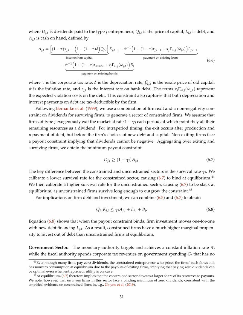
where Dj,t is dividends paid to the type j entrepreneur, Qj,t is the price of capital, Lj,t is debt, andAj,t is cash on hand, defined by

Aj,t =[(1− τ)xj,t +

(1− (1− τ)δ

)Qj,t

]︸ ︷︷ ︸

income from capital

Kj,t−1 − π−1(

1 + (1− τ)rj,t−1 + κjΓω,j(ωj,t))

Lj,t−1︸ ︷︷ ︸payment on existing loans

− π−1(

1 + (1− τ)rbond,t + κjΓω,j(ωj,t))

Bj︸ ︷︷ ︸payment on existing bonds

(6.6)

where τ is the corporate tax rate, δ is the depreciation rate, Qj,t is the resale price of old capital,π is the inflation rate, and rj,t is the interest rate on bank debt. The terms κjΓω,j(ωj,t) representthe expected violation costs on the debt. This constraint also captures that both depreciation andinterest payments on debt are tax-deductible by the firm.

Following Bernanke et al. (1999), we use a combination of firm exit and a non-negativity con-straint on dividends for surviving firms, to generate a sector of constrained firms. We assume thatfirms of type j exogenously exit the market at rate 1− γj each period, at which point they all theirremaining resources as a dividend. For intraperiod timing, the exit occurs after production andrepayment of debt, but before the firm’s choices of new debt and capital. Non-exiting firms facea payout constraint implying that dividends cannot be negative. Aggregating over exiting andsurviving firms, we obtain the minimum payout constraint

Dj,t ≥ (1− γj)Aj,t. (6.7)

The key difference between the constrained and unconstrained sectors is the survival rate γj. Wecalibrate a lower survival rate for the constrained sector, causing (6.7) to bind at equilibrium.44

We then calibrate a higher survival rate for the unconstrained sector, causing (6.7) to be slack atequilibrium, as unconstrained firms survive long enough to outgrow the constraint.45

For implications on firm debt and investment, we can combine (6.5) and (6.7) to obtain

Qj,tKj,t ≤ γj Aj,t + Lj,t + Bj. (6.8)

Equation (6.8) shows that when the payout constraint binds, firm investment moves one-for-onewith new debt financing Lj,t. As a result, constrained firms have a much higher marginal propen-sity to invest out of debt than unconstrained firms at equilibrium.

Government Sector. The monetary authority targets and achieves a constant inflation rate π,while the fiscal authority spends corporate tax revenues on government spending Gt that has no

44Even though many firms pay zero dividends, the constrained entrepreneur who prices the firms’ cash flows stillhas nonzero consumption at equilibrium due to the payouts of exiting firms, implying that paying zero dividends canbe optimal even when entrepreneur utility is concave.

45At equilibrium, (6.7) therefore implies that the constrained sector devotes a larger share of its resources to payouts.We note, however, that surviving firms in this sector face a binding minimum of zero dividends, consistent with theempirical evidence on constrained firms in, e.g., Cloyne et al. (2019).

31

effect on household utility.

Entrepeneurs’ Problems. The unconstrained and constrained entrepreneurs choose consump-tion Cj,t to maximize (6.1) subject to the budget constraint Cj,t ≤ Dj,t.

Firm’s Problem. The sector-type j firm maximizes (6.4) subject to (6.5) and (6.8).

Bank’s Problem. Each banking sector b contains a continuum of competitive banks that lend toa set of firms Sb, pays a convex funding cost, and returns the proceeds to the saver as a dividendDS,b,t. The representative bank in sector b solves the problem

Vb,t = max DS,b,t + Et [ΛS,t+1Vb,t+1]

subject to

DS,b,t ≤ π−1 (1 + rb,t−1) Lb,t−1 − Lb,t︸ ︷︷ ︸net lending income

−(

η

1 + ζL

)(Lb,t

Lb

)1+ζL

︸ ︷︷ ︸funding cost

where Lb,t is total lending to all types of firms, and Lb is its steady state value.Each bank’s optimality condition with respect to Lb,t is

(1 + rb,t) = (1 + rt)︸ ︷︷ ︸risk-free rate

(1 + sb,t)︸ ︷︷ ︸spread

, sb,t ≡ η

(Lb,t

Lb

)ζL

. (6.9)

When unconstrained and constrained firms are mixed in the set Sb, (6.9) implies that borrowingby one type raises spreads for the other type, inducing crowding out.

In our version of the model in which unconstrained firms have access to credit lines, theirinterest rate is instead given by

(1 + rt) = (1 + rt)(1 + s) (6.10)

where the constant s represents the predetermined spreads on credit lines facilities.For the matching structure Sb, we assume that each firm is randomly matched with a banking

sector b for their term lending. Absent credit lines, all banking sectors would therefore be sym-metric. However, for the model with credit lines, we assume that undrawn credit line capacity,and therefore drawdowns, vary across banking sectors (see Appendix A.2 for details). This cross-sectional variation allows us to replicate our empirical regression (5.3) in our calibration below.

32

Saver’s Problem. The saver chooses consumption CS,t and labor to each firm NS,i,t, and risk-freebonds At to maximize (6.2) subject to the budget constraint

CS,t ≤ wtNS,t +∫

bDS,b,t dΓb(b)︸ ︷︷ ︸

bank dividends

+ (1 + rt−1)π−1At−1 − At︸ ︷︷ ︸

risk-free bonds

+(

π−1(1 + rbond,t−1)− 1)

B︸ ︷︷ ︸corporate bonds

+ TS,t︸︷︷︸rebate

.

where At denotes risk-free bonds in zero net supply, B = BU + BC denotes total corporate bonds,and TS,t rebates the funding cost lump sum to savers to ensure that this cost has no effect on theeconomy’s total supply of resources.

Capital Producers. Competitive producers create capital for each sector using

Kj,t = Φ(ij,t)Kj,t−1 + (1− δ)Kj,t−1

where ij,t = Ij,t/Kj,t−1 is the share of investment expenditures to existing capital in sector j. Thecapital producers buy existing capital at price Qj,t and sell new capital at price Qj,t. The capitalproducer’s problem is therefore given by

maxij,t,Kj,t−1

Qj,t

[Φ(ij,t)Kj,t−1 + (1− δ)Kj,t−1

]− ij,tKj,t−1 − Qj,t(1− δ)Kj,t−1.

Final Good Producers. The intermediate goods from each sector are packaged by competitivefinal goods producers using the technology

Yt =

(χUY

εy−1εy

U,t + χC

∫b

Yεy−1

εyC,b,t dΓb(b)

) εyεy−1

where χU and χC are the measures of unconstrained and constrained firms, respectively. The priceof the final good is normalized to unity, while the price of the intermediate good produced by firmj is Pj,t. Combining, the final good producer’s problem is

maxYj,t

(∫jY

εy−1εy

j,t

) εyεy−1

−∫

jPj,tYj,t.

6.3 Equilibrium

Competitive equilibrium in this model is an allocation of endogenous states (Kj,t, X∗j,t, rj,t), policies(Nj,t, ij,t, nS,t, At), and prices (rj,t, Qj,t, Qj,t, rt, Pj,t, , wt), for j ∈ {U, (C, b)}, such that all agents’problems are optimized, and the markets for labor, capital goods, intermediate goods, final goods,and loans all clear. We provide (6.9) and (6.10) in the main text above, and relegate the remainingequilibrium conditions to Appendix A.1.

33

6.4 Calibration

Our quarterly calibration is displayed in Table 6.1. To stay parallel to our empirical findings, wematch unconstrained firms to data on firms in the top 10% of the size distribution and constrainedfirms to data on firms in the bottom 90% of the size distribution.

Table 6.1: Parameter Values: Baseline Calibration (Quarterly)

Parameter Name Value Internal Target/Source

Preferences

Entrepreneur Discount Factor (U) βU 0.992 N See textEntrepreneur Discount Factor (C) βC 0.992 N See textEntrepreneur RRA (U) ψU 0.01 N See textEntrepreneur RRA (C) ψC 0.01 N See textSaver Discount Factor βS 0.995 N See textSaver Labor Disutility ϕ 0.5 N StandardSaver Labor Disutility ν 0.536 Y N = 1

Funding Cost

Funding Cost Curvature ζL 4.606 N See textFunding Cost Level η 0.625% Y 250bp Spread (Ann.)Credit Line Spread s 0.625% N 250bp Spread (Ann.)Bond Spread sbond 0.625% N 250bp Spread (Ann.)

Financial

Minimum Payout 1− γC 0.02 N See textMinimum Payout 1− γU 0.00 N See textDebt-to-EBITDA Limit θ 15 N DealscanCovenant Smoothing ρL 0.75 N 4Q smoothingCovenant Violation Fee (U) κU 0.000272 N See textCovenant Violation Fee (C) κC 0.0253 N See textIdio. EBITDA Vol. (U) σω,U 0.660 N See textIdio. EBITDA Vol. (C) σω,C 0.882 N See textCorporate Bonds (U) BU 2.944 N See textCorporate Bonds (C) BC 0 N See text

Technology and Government

Capital Share α 0.33 N StandardCapital Adjustment Cost ζK 0.5 N StandardVariety Elasticity εy 6 N See textLabor Sector Elasticity εn 6 N See textUnconstrained Share aU 0.752 N Asset sharesProductivity log Z -0.715 Y Y = 1Productivity ρZ 0.75 N SPF ForecastCorporate Tax Rate τ 0.21 N StandardInflation Rate π 1.005 N 2% inflation

34

Preferences. We assume that constrained and unconstrained entrepreneurs have the same pref-erence parameters, so that the only difference between the two types come from their exit ratesand credit technologies. Our preference specification requires calibration of two parameters, ψ

and β, which control the entrepreneur dividend smoothing incentive and discount factor, respec-tively. In principle, we could calibrate these parameters to match the growth in payouts and creditover the COVID-19 episode. However, it turns out that our model is unable to fully match thedecline in payouts or rise in credit for any feasible value of these parameters, given our remainingcalibration strategy. We believe this is due to a strong precautionary motive to amass financialresources in uncertain times that is not present in our model’s perfect foresight experiments. Asa result, we instead choose each parameter to get as close as possible to the true moments withinthat parameter’s feasible range. We note that in both cases our core results strengthen as we getcloser to the true data moment, implying our results are likely conservative.

For the β parameters, our baseline calibration βU = βC = 0.992 falls at the upper end of thefeasible range, implying that unconstrained firms are close to indifferent between borrowing andinternal finance. For the ψ parameters, our baseline calibration ψU = ψC = 0.01 falls at the lowerend of the feasible range, representing a weak but nonzero motivation to smooth payouts. Thisweak smoothing incentive reflects the various flexible financial margins available to large firms,such as repurchasing stock, spending out of cash, and issuing new non-bank debt. Further detailsabout the calibration of these parameters, as well as sensitivity results using a range of parametersfor both ψ and β, can be found in Appendix A.5.

For the saver, we set βS to 0.995 to target a steady state annualized real discount rate of 2%.Saver labor disutility is calibrated so that ϕ, the inverse Frisch elasticity, is equal to 0.5, while themultiplicative term χ is set so that N = 1 in steady state.

Funding Cost. We next calibrate the funding cost parameters. The key parameter here is theelasticity ζL, which determines the strength of the crowding out effect. We calibrate this parameterso that estimating the cross-sectional regression (5.3) on constrained firms in the model deliversthe exact coefficient implied by Table 5.2, yielding a value of 4.606. Full details on this procedurecan be found in Appendix A.2. Once we have obtained our value for ζL, the coefficient η is setto ensure a steady-state spread of 250bp, while s and sbond are chosen to ensure the same 250bpspread on credit lines and corporate bonds, respectively. For intuition, these parameters implythat a 1% increase in bank-firm credit raises credit spreads on bank loans by 11.7bp. Finally, forbanking sector heterogeneity, we assume in our benchmark economy that log undrawn credit linebalances (and therefore log credit line draws) are normally distributed across banking sectors withstandard deviation σb = 0.914, calibrated to match the dispersion across banks in our sample.

Financial. We set the exit rate for unconstrained firms to zero, and set the exit rate for constrainedfirms to 2 percent, close to the value used in Bernanke et al. (1999). For the debt covenants, wechoose a debt-to-EBITDA limit of 3.75 (annual), in line with the evidence in Greenwald (2019). We

35

set the smoothing parameter ρL to 0.75, consistent with covenants averaging EBITDA over fourquarters. We parameterize the ωi,t distribution as a lognormal, so that

log ωj,t ∼ N(−1

2σ2

ω,j, σ2ω,j

).

We calibrate the violation costs κU , κC and the idiosyncratic volatilities σω,U and σω,C for eachsector to match four targets: the ratio of debt to capital in each sector, equal to 32% for the uncon-strained sector, and 28% for the constrained sector; and the rate at which firms exceed the modeldebt-to-EBITDA threshold of 15 (quarterly), equal to 34% for the unconstrained sector and 32% forthe constrained sector, rates similar to those found in Chodorow-Reich and Falato (2021). Exper-imenting with alternative values for these parameters had little influence on the results providedthey yielded reasonable values for firm leverage. Finally, we assume that constrained firms do notissue corporate bonds (BC = 0) and choose the level of bonds held by unconstrained firms (BU) toensure that 40% of bank debt is held by the unconstrained sector in steady state, consistent withthe share held by the 10% largest firms in the Y14 data.46

Technology and Government. We set the capital share to α = 0.33, a standard value. We param-eterize the investment adjustment cost as

Φ(ij,t) = φ0 + φ1i1−ζKj,t

1− ζK.

We set ζK = 0.5, which is in the typical range used by the literature and generates a reasonableinvestment response to a TFP decline. For the other coefficients, we set

φ0 = δ

(ζK

ζK − 1

), φ1 = δζK

to ensure that Φ(i) = i and Φ′(i) = 1 in steady state.For productivity, we set the average level Z so that steady-state output is normalized to unity,

and the persistence φZ = 0.75 to match the COVID-19 output scenario implied by the 2020:Q2Survey of Professional Forecasters.47 For the final goods aggregator, we choose a typical elasticityvalue εy = 6 and symmetrically set εn = 6. Experimentation has shown that these elasticityparameters are quantitatively unimportant for our main results. We choose the weights aU = 0.752and aC = 1− aU , so that unconstrained firms account for 86% of sales in steady state, consistentwith the share produced by the top 10% largest firms in our data.

46Assuming that the constrained sector holds a positive amount of corporate bonds would require us to assign alarger share of bonds to the unconstrained sector, implying that the proportional growth of bank credit would be evenlarger over the COVID-19 episode. We therefore consider this to be a conservative calibration.

47This forecast projected 2020:Q2 output growth of -32.2 percent and 2020:Q3 output growth of 10.6 percent, bothannualized. The implied quarterly log growth rates are -0.0972 and 0.0252, respectively. Under an AR(1) processbeginning from steady state, these rates should correspond to εZ,t and −(1 − φZ)εZ,t, respectively. Solving for twoequations in two unknowns yields φZ = 0.741.

36

For the government sector we set τ to 0.21, matching the US corporate tax rate, and the inflationrate to 1.005, implying an annual inflation rate of 2%.

6.5 Results

We study the response of the economy to an adverse TFP shock, designed to mimic the COVID-19 episode. Specifically, we compute perfect foresight paths in response to the unexpected shockεZ = −0.0552, a magnitude chosen to match the decline in GDP in 2020:Q2 in our benchmark(“Credit Lines”) specification.48 For each experiment, we apply an unexpected shock, then tracethe nonlinear transition back to steady state.

To shed light on the specific contributions of the credit line channel and of cross-type spilloversmore generally, we compare outcomes under two different models. To set a baseline, we considera “Term Loans” economy in which all firms borrow in one period debt at the current marketspread, given by (6.9). From this starting point, we move to a “Credit Lines” economy in whichunconstrained firms borrow on credit lines at a fixed spread according to (6.10), while constrainedfirms borrow using term loans at the current market spread according to (6.9).

We begin with Figure 6.1, which shows the separate responses for unconstrained (U) and con-strained (C) firms in each economy, where results for constrained firms aggregate over all possiblebanking sectors b. To set a baseline, we can begin with the Term Loans economy. Following anegative shock to TFP, profits fall for both types of firms. As a result, each firm is forced to adjustby balancing three costly margins: (i) cutting dividends (if unconstrained), subject to dividendsmoothing motives; (ii) cutting investment, subject to adjustment costs; or (iii) increasing debt,subject to increasing expected violation costs.

Importantly, unconstrained firms are able to adjust their dividend, and do so heavily, reducingdividends 35.7% on impact. As a result, unconstrained firms are able to balance their budgetconstraint with only a very small decline in investment, with capital falling by only 0.18% overthe 20Q following the shock. In contrast, constrained firms already face a binding minimum fordividends, and cannot voluntarily cut them further.49 Instead, constrained firms are forced to cutinvestment, leading to a much larger drop in capital of 0.74% in the 20Q following the shock.

At equilibrium, unconstrained firms also have a more price sensitive demand for debt, sincethey would rather reduce their dividend than pay high spreads. In contrast, constrained firmshave a more inelastic demand for debt, since decreasing debt requires them to cut investment —a more costly margin of adjustment. At equilibrium, this drives constrained firms to substantiallyincrease their borrowing following the shock, while unconstrained firms cut their borrowing by asimilar margin to avoid the increase in spreads. As a result, the Term Loans economy delivers arelative flow of credit from unconstrained toward constrained firms following the negative shock,generating the opposite pattern compared to what we observed empirically in Figure 5.2.

48This decline in productivity is smaller than the 9.5 percent target drop in GDP due to the endogenous reductionin labor hours, which amplifies the impact of the shock on output.

49Constrained firm payouts still exhibit some decline due to the lower values of exiting firms.

37

0 5 10 15 20

0

10

20

Bank Debt (U)

0 5 10 15 200.2

0.1

0.0Capital (U)

0 5 10 15 20

30

20

10

0Dividends (U)

0 5 10 15 20Quarters

5

0

Bank Debt (C)

0 5 10 15 20Quarters

3

2

1

0Capital (C)

0 5 10 15 20Quarters

7.5

5.0

2.5

0.0Dividends (C)

Credit LinesTerm Loans

Figure 6.1: Responses by Type, Credit Line vs. Term Loan Economies

Notes: This figure plots the impulse response to the productivity shock εZ = −0.0552. Variable definitions are asfollows: “Debt (U)” is LU,t; “Capital (U)” is KU,t; “Dividends (U)” is DU,t; “Debt (C)” is LC,t; “Capital (C)” is KC,t;“Dividends (C)” is DC,t. All variables are in logs and are displayed in percent.

From this baseline, we now turn to the Credit Lines economy, which allows unconstrainedfirms, and only unconstrained firms, to borrow through credit lines at a fixed spread s. Figure6.2 shows that unconstrained firms now increase, rather than decrease their borrowing. Althoughunconstrained firms are still highly sensitive to the price of credit, the fixed spread on credit linesinsulates them from any rising spreads. As a result, unconstrained firms now primarily adjustby borrowing much more (at ex-post underpriced rates), while decreasing their dividend payoutnearly four times less on impact (4.6%) as in the Term Loans economy. Unconstrained firm invest-ment is largely unaffected by the inflow of credit, falling by a virtually identical 0.14% after 20Q,demonstrating these firms’ low marginal propensities to invest.

This large increase in unconstrained firm borrowing puts pressure on bank balance sheets dueto banks’ convex funding costs, raising the spreads on new debt and crowding out borrowingby constrained firms. Constrained firm borrowing now falls where it had previously risen inthe Term Loans economy. Since constrained firms are forced to offset this change in debt withreduced investment, their capital now falls by roughly five times more after 20Q compared to theTerm Loans economy (3.16% vs. 0.74%).

38

0 5 10 15 2010

5

0Output

0 5 10 15 20

0.4

0.2

0.0Capital

0 5 10 15 20

20

10

0Dividends

0 5 10 15 20Quarters

0.0

2.5

5.0

7.5Bank Debt

0 5 10 15 20Quarters

0.0

0.5

1.0

Spread

0 5 10 15 20Quarters

0.0

2.5

5.0

Bank Debt Share (U)

Credit LinesTerm Loans

Figure 6.2: Aggregate Responses, Credit Line vs. Term Loan Economies

Notes: This figure plots the impulse response to the shock εZ = −0.0552. Variable definitions are as follows: “Out-put” is Yt; “Capital” is aUKU,t + aCKC,t; “Dividends” is aU DU,t + aCDC,t; “Debt” is aU LU,t + aC LC,t; “Spread” is sC,t,equivalently sU,t in the All Unconstrained and Term Loans economies; “Debt Share (U)” is aU LU,t/(aU LU,t + aC LC,t).The responses of “Spread” and “Debt Share (U)” are displayed in levels in percentage points, while the responses ofthe remaining variables are displayed in logs in percent.

To study the model’s macroeconomic implications, Figure 6.2 displays aggregate series for ourTerm Loans and Credit Lines economies. The bottom left panel shows that the introduction ofcredit lines substantially increases aggregate debt issuance following the negative shock, peakingat over 7% growth, compared to just over 1% peak growth in the Term Loans economy. Thisoccurs because unconstrained firms borrow much more than in the Term Loans economy, whilethe highly inelastic credit demand of the constrained firms does not fall sufficiently to offset it.Further, the bottom right panel shows that the addition of credit lines causes credit to flow towardunconstrained firms following the shock, matching our empirical findings. The model thereforeimplies that credit lines were central to both the aggregate and cross-sectional patterns observedfollowing the outbreak of COVID-19 in Figures 1.2 and 5.2.

Despite boosting aggregate credit growth, credit lines worsen aggregate disinvestment fol-lowing this shock. Figure 6.2 shows that aggregate capital falls by 0.56% in the 20Q followingthe shock, nearly tripling the decline in the Term Loan economy (0.26%). Although total credit is-suance is larger compared to the Term Loans economy, credit lines lead to a large transfer of credit

39

from constrained firms, who have the highest marginal propensities to invest in the economy, to-ward unconstrained firms, who have the lowest. As a result, the decline in investment by theconstrained firms is not offset by increases in investment by the unconstrained firms, who investvirtually none of these resources. Instead, larger credit flows to unconstrained firms primarilyprop up aggregate dividends, which now fall by 6.0% on impact, a decline more than four timesless than observed in the Term Loans economy (23.8%).

In summary, our model indicates that credit lines are structurally important to the patterns weobserved in the data, and that it would be challenging to replicate the strong flow of bank credittoward unconstrained firms in bad times without them. But despite increasing overall lendingto the corporate sector in bad times, the fact that these credit lines are overwhelmingly held byunconstrained firms can worsen the economic consequences of the recession. In closing, we notethat while our model lacks any mechanism for this channel to influence output beyond excessivedisinvestment, parallel phenomena could easily occur if constrained firms were forced to losematch surplus by laying off workers or destroy value by inefficiently liquidating in default. Asa result, we believe our quantitative results could be substantially amplified by considering theimpact of these countercyclical credit flows in richer models of firm production and investment.

6.6 Extensions

This section presents several extensions to our baseline model. We summarize the specificationsand results here, and relegate additional details to Appendix A.

Cash Holdings. While our baseline model abstracts from cash holdings for parsimony, in prac-tice cash represents an alternative store of precautionary resources that small firms could use tosmooth investment following an adverse shock. In Appendix A.3, we extend the model to allowboth types of firms to hold cash. Since our results largely hinge on how flexibly cash is used tosmooth investment, we proxy for the precautionary value of cash using a simple specification inwhich cash enters the utility function of the firm, so that the curvature of utility from cash willmap directly into the flexibility of this margin. Our estimates in Tables 5.2 and F.10 imply thatsmall firms react to crowding out by reducing investment and cash holdings equally, we repro-duce these IV estimates in the model, and calibrate the key curvature parameter so that the modelexactly reproduces the equality of these IV coefficients.50

The impulse responses from the model with cash, shown in Figure A.1, illustrate that theability of small firms to spend down cash does reduce the quantitative fall in investment, with theaggregate capital stock now falling by 0.39% rather than 0.56% after 20Q. However, this decline

50Both of these IV coefficients are 0.12 in the model, reasonably close to the 0.07 found in the data. To the extentthat the difference is due to a decline in resources used for productive purposes such as working capital, or representsfuture investment delayed by time-to-build frictions not present in the model, the model with cash will somewhatunderestimate the strength of the credit line channel. To the extent that the difference is instead accounted for bydecreased dividend payouts by small firms, the model with cash will somewhat overestimate the strength of the creditline channel. This distinction would require additional data and is left for future work.

40

in the capital stock in the Credit Lines economy with cash is still more than 60% larger than thecorresponding 0.24% decline in the Term Loans economy with cash, due to the influence of thecredit line channel. As a result, we conclude that the cash margin is quantitatively relevant, butinsufficient to fundamentally alter our core results based on our empirically estimated elasticities.

Bond Market Interventions. Although our model correctly captures a strong rise in bank-firmcredit following the outbreak of COVID-19, it predicts that bank-firm credit remains elevated forseveral years. In the data, however, much of the change in bank-firm credit following the COVID-19 outbreak reverted by 2020:Q3. We believe that this discrepancy is due to changes in bondmarket conditions, largely due to interventions by the Federal Reserve, that restored bond mar-kets as a conduit for large firms to obtain credit at affordable rates. The resulting wave of bondissuance, which increased the stock of corporate bonds by over 7% between 2020:Q1 and 2020:Q2,substituted for bank credit, allowing large firms to pay down their credit line balances (Darmouniand Siani, 2020).

To investigate this in the context of our model, Appendix A.4 extends our framework to allowour previously static bond holdings Bj to instead follow a stochastic process. Figure A.2 showsthat a modest increase in bond holdings can lead large firms to fully pay down their credit lines,as observed in the data. Importantly, this repayment removes pressure on bank balance sheets,alleviating the crowding out effects harming small firms and increasing aggregate investment.We therefore conclude that one of the most important effects of bond market interventions mayhave been indirect, by improving credit access to small firms that do not use corporate bonds, butnonetheless benefited from better access to bank term lending.

Still, aggregate capital and constrained firm debt remain persistently depressed in the BondMarket Shock extension relative to the Term Loans economy without credit lines. Since con-strained firms have already disinvested substantially by the intervention date, capital adjustmentcosts and tighter covenant limits due to lower EBITDA prevent them from rapidly reaccumulatingdebt and investment. These results imply that ex-post bond market interventions may not be acomplete solution, and may also explain why we find continuing crowding out effects in 2020:Q3,even after many credit lines have been repaid.

7 Conclusion

In this paper, we have argued that credit lines are central to the transmission of macroeconomicshocks to firm credit, at both the aggregate and cross-sectional levels. Using a highly granular dataset, we are able to open the black box of U.S. bank balance sheets to show that unused credit linecapacity is vast, but overwhelmingly concentrated among the largest, least financially constrainedfirms. As a result, while credit lines allow for a large expansion of aggregate firm credit followingadverse shocks, they also crowd out credit to constrained firms in favor of unconstrained firms,potentially depressing firm investment. Our theoretical results show that the predetermined pric-

41

ing and terms of credit lines are key to this relative flow of credit, which would otherwise favorconstrained firms following adverse shocks to productivity. Moreover, this cross-sectional pat-tern has important aggregate implications, severely worsening the drop in investment followingnegative shocks, despite increasing the aggregate flow of credit.

Looking ahead, our work has implications for both research and policy. On the research side,workhorse macroeconomic models, such as Bernanke et al. (1999) and Kiyotaki and Moore (1997),impose that the corporate sector is financially constrained, and is either unable to borrow furtheror dissuaded from doing so by rising credit spreads. Our data show instead that, in the aggregate,the corporate sector is far from constrained, with access to large amounts of unused credit underpredetermined conditions. The financial accelerator mechanism therefore depends crucially onthe allocation of credit across the firm distribution, and not merely on aggregate quantities. Weencourage researchers to view the reallocation of credit between firms as of primary importancein driving macrofinancial dynamics.

For policymakers, these findings highlight the potential risks inherent in banks’ undrawncredit lines. Because committed credit line balances have lower risk weights when undrawn, asudden wave of drawdowns can tie up bank capital in bad times, leading banks to reduce otherlending in an attempt to improve their capital ratios. Regulatory treatment of unused credit capac-ity should be carefully calibrated to account for these macroeconomic externalities. Our findingscould also motivate various policy interventions during severe crises, particularly ones that di-rectly provide credit to SMEs, such as the Paycheck Protection Program. Finally, the effects thatwe document could have been even stronger without some of the policy interventions put in placeover the COVID-19 outbreak period. For example, we find that a quick recovery in the corporatebond market may have had strong indirect effects by improving bank credit conditions for smallfirms that do not issue corporate bonds. To the extent that this recovery was due to Federal Re-serve interventions, our results provide additional motivation for such a policy.

Overall, the central role of credit lines in driving credit flows in bad times makes them a highlysalient target for future academic and policy research.

References

Acharya, Viral, Heitor Almeida, and Murillo Campello, 2013, Aggregate risk and the choice between cashand lines of credit, The Journal of Finance 68, 2059–2116.

Acharya, Viral, Heitor Almeida, Filippo Ippolito, and Ander Pérez Orive, 2014, Credit lines as monitoredliquidity insurance: Theory and evidence, Journal of Financial Economics 112, 287–319.

Acharya, Viral, Heitor Almeida, Filippo Ippolito, and Ander Pérez Orive, 2019, Bank lines of credit ascontingent liquidity: Covenant violations and their implications, Journal of Financial Intermediation 44,100817.

Acharya, Viral, Heitor Almeida, Filippo Ippolito, and Ander Pérez Orive, 2021a, Credit lines and the liq-uidity insurance channel, Journal of Money, Credit, and Banking 53, 901–938.

Acharya, Viral, Robert Engle, and Sascha Steffen, 2021b, Why did bank stocks crash during covid-19?,Unpublished Manuscript. NYU Stern .

42

Acharya, Viral, and Sascha Steffen, 2020, The risk of being a fallen angel and the corporate dash for cash inthe midst of covid, COVID Economics 10, 44–61.

Anderson, Gareth, and Ambrogio Cesa-Bianchi, 2020, Crossing the credit channel: credit spreads and firmheterogeneity, Unpublished working paper, Bank of England .

Ashcraft, Adam B., 2005, Are banks really special? new evidence from the fdic-induced failure of healthybanks, American Economic Review 95, 1712–1730.

Bahaj, Saleem, Angus Foulis, Gabor Pinter, and Paolo Surico, 2020, Employment and the collateral channelof monetary policy, Unpublished working paper, Bank of England .

Barraza, Santiago, Andrea Civelli, and Nicola Zaniboni, 2019, Business loans and the transmission of mon-etary policy, Journal of Financial and Quantitative Analysis 54, 925–965.

Berg, Tobias, Anthony Saunders, and Sascha Steffen, 2016, The total cost of corporate borrowing in the loanmarket: Don’t ignore the fees, The Journal of Finance 71, 1357–1392.

Berg, Tobias, Anthony Saunders, Sascha Steffen, and Daniel Streitz, 2017, Mind the gap: The differencebetween us and european loan rates, The Review of Financial Studies 30, 948–987.

Bernanke, Ben, Mark Gertler, and Simon Gilchrist, 1999, The financial accelerator in a quantitative businesscycle framework, Chap. 21 in Handbook of Macroeconomics, ed. J. B. Taylor and M. Woodford. Amsterdam:Elsevier. 1C.

Bernanke, Ben S., and Mark Gertler, 1995, Inside the black box: The credit channel of monetary policytransmission, Journal of Economic Perspectives 9, 27–48.

Berrospide, Jose, and Ralf Meisenzahl, 2015, The real effects of credit line drawdowns, Finance and EconomicDiscussion Series 2015-007, Board of Governors of the Federal Reserve System (U.S.) .

Bidder, Rhys, John Krainer, and Adam Shapiro, 2020, De-leveraging or de-risking? how banks cope withloss, Review of Economic Dynamics .

Blattner, Laura, Luísa Farinha, and Francisco Rebelo, 2020, When losses turn into loans: The cost of weakbanks, Unpublished Manuscript, Stanford .

Brown, James, Matthew Gustafson, and Ivan Ivanov, 2020, Weathering cash flow shocks, Journal of Finance,forthcoming .

Caglio, Cecilia, Matthew Darst, and Sebnem Kalemli-Özcan, 2021, Risk-taking and monetary policy trans-mission: Evidence from loans to smes and large firms, NBER Working Paper .

Campello, Murillo, Erasmo Giambona, John R. Graham, and Campbell Harvey, 2011, Liquidity manage-ment and corporate investment during a financial crisis, Review of Financial Studies 24, 1944–1979.

Campello, Murillo, John Graham, and Campbell Harvey, 2010, The real effects of financial constraints:Evidence from a financial crisis, Journal of Financial Economics 97, 470–487.

Chari, Varadarajan, Lawrence Christiano, and Patrick Kehoe, 2008, Facts and myths about the financialcrisis of 2008, Federal Reserve Bank of Minneapolis, Unpublished working paper .

Chodorow-Reich, Gabriel, 2014, The employment effects of credit market disruptions: Firm-level evidencefrom the 2008-09 financial crisis, Quarterly Journal of Economics 129, 1–59.

Chodorow-Reich, Gabriel, Olivier Darmouni, Stephan Luck, and Matthew Plosser, 2020, Bank liquidityprovision across the firm size distribution, NBER Working Paper .

Chodorow-Reich, Gabriel, and Antonio Falato, 2021, The loan covenant channel: How bank health trans-mits to the real economy, Journal of Finance, Forthcoming .

43

Christiano, Lawrence J., Martin Eichenbaum, and Charles L. Evans, 2005, Nominal Rigidities and the Dy-namic Effects of a Shock to Monetary Policy, Journal of Political Economy 113, 1–45.

Cloyne, James, Clodomiro Ferreira, Maren Froemel, and Paolo Surico, 2019, Monetary policy, corporatefinance and investment, Unpublished working paper, Bank of Spain .

Cohen-Cole, Ethan, Burcu Duygan-Bump, Jose Fillat, and Judit Montoriol-Garriga, 2008, Looking behindthe aggregates: a reply to "facts and myths about the finacial crisis", Federal Reserve Bank of Boston, Un-published working paper .

Coibion, Olivier, 2012, Are the effects of monetary policy shocks big or small?, American Economic Journal:Macroeconomics 4, 1–32.

Coibion, Olivier, Yuriy Gorodnichenko, Lorenz Kueng, and John Silvia, 2017, Innocent bystanders? mone-tary policy and inequality in the u.s, Journal of Monetary Economics 88, 70–89.

Cornett, Marcia, Jamie McNutt, Philip Strahan, and Hassan Tehranian, 2011, Liquidity risk managementand credit supply in the financial crisis, Journal of Financial Economics 101, 297–312.

Crouzet, Nicolas, and Neil Mehrotra, 2020, Small and large firms over the business cycle, American EconomicReview 110, 3549–3601.

Darmouni, Olivier, Oliver Giesecke, and Alexander Rodnyansky, 2020, The bond lending channel of mon-etary policy, CEPR Discussion Paper .

Darmouni, Olivier, and Kerry Siani, 2020, Crowding out bank loans: Liquidity-driven bond issuance, Un-published Manuscript, Columbia University .

Demiroglu, Cem, and Christopher James, 2011, The use of bank lines of credit in corporate liquidity man-agement, Journal of Banking and Finance 35, 775–782.

den Haan, Wouter, Steven Sumner, and Guy Yamashiro, 2007, Bank loan portfolios and the monetary trans-mission mechanism, Journal of Monetary Economics 54, 904–924.

Drechsler, Itamar, Alexi Savov, and Philipp Schnabl, 2017, The deposits channel of monetary policy, TheQuarterly Journal of Economics 132, 1819–1876.

Driscoll, John C., and Aart C. Kraay, 1998, Consistent covariance matrix estimation with spatially dependentpanel data, The Review of Economics and Statistics 80, 549–560.

Field, Laura Casares, and Jonathan M. Karpoff, 2002, Takeover defenses of ipo firms, The Journal of Finance57, 1857–1889.

Gan, Jie, 2007, The real effects of asset market bubbles: Loan- and firm-level evidence of a lending channel,Review of Financial Studies 20, 1941–1973.

Gatev, Evan, and Philip Strahan, 2006, Banks’ advantage in hedging liquidity risk: Theory and evidencefrom the commercial paper market, The Journal of Finance 61, 867–892.

Gertler, Mark, and Simon Gilchrist, 1993a, The cyclical behavior of short-term business lending: Implica-tions for financial propagation mechanisms, European Economic Review 37, 623–631.

Gertler, Mark, and Simon Gilchrist, 1993b, The role of credit market imperfections in the monetary trans-mission mechanism: arguments and evidence, Scandinavian Journal of Economics 95, 43–64.

Gertler, Mark, and Simon Gilchrist, 1994, Monetary policy, business cycles, and the behavior of small man-ufacturing firms, The Quarterly Journal of Economics 109, 309–340.

Gilchrist, Simon, and Egon Zakrajšek, 2012, Credit spreads and business cycle fluctuations, American Eco-nomic Review 102, 1692–1720.

44

Gomez, Matthieu, Augustin Landier, David Sraer, and David Thesmar, 2020, Banks exposure to interestrate risk and the transmission of monetary policy, Journal of Monetary Economics .

Granja, João, Christos Makridis, Constantine Yannelis, and Eric Zwick, 2020, Did the paycheck protectionprogram hit the target?, NBER Working Paper .

Greenwald, Daniel, 2019, Firm debt covenants and the macroeconomy: The interest coverage channel,Unpublished Manuscript, MIT .

Gürkaynak, Refet, Brian Sack, and Eric Swanson, 2005, Do Actions Speak Louder Than Words? The Re-sponse of Asset Prices to Monetary Policy Actions and Statements, International Journal of Central Banking1, 55–93.

Herreño, Juan, 2020, The aggregate effects of bank lending cuts, Unpublished working paper, Columbia Uni-versity .

Holmström, Bengt, and Jean Tirole, 1998, Private and public supply of liquidity, Journal of Political Economy106, 1–40.

Huber, Kilian, 2018, Disentangling the effects of a banking crisis: Evidence from german firms and counties,American Economic Review 108, 868–898.

Ippolito, Filippo, José-Luis Peydró, Andrea Polo, and Enrico Sette, 2016, Double bank runs and liquidityrisk management, Journal of Financial Economics 122, 135–154.

Ivashina, Victoria, and David Scharfstein, 2010, Bank lending during the financial crisis of 2008, Journal ofFinancial Economics 97, 319–338.

Iyer, Rajkamal, José-Luis Peydró, Samuel da Rocha-Lopes, and Antoinette Schoar, 2014, Interbank liquiditycrunch and the firm credit crunch: Evidence from the 2007–2009 crisis, Review of Financial Studies 27,347–372.

Jarocinski, Marek, and Peter Karadi, 2020, Deconstructing monetary policy surprises: the role of informa-tion shocks, American Economic Journal: Macroeconomics 12, 1–43.

Jeenas, Priit, 2019, Monetary policy shocks, financial structure, and firm activity: A panel approach, Unpub-lished working paper .

Jiménez, Gabriel, Jose A Lopez, and Jesús Saurina, 2009, Empirical analysis of corporate credit lines, TheReview of Financial Studies 22, 5069–5098.

Jiménez, Gabriel, Atif Mian, José-Luis Peydró, and Jesús Saurina, 2020, The real effects of the bank lendingchannel, Journal of Monetary Economics 115, 162–179.

Jiménez, Gabriel, Steven Ongena, José-Luis Peydró, and Jesús Saurina, 2012, Credit supply and monetarypolicy: Identifying the bank balance-sheet channel with loan applications, American Economic Review 102,2301–26.

Jiménez, Gabriel, Steven Ongena, José-Luis Peydró, and Jesús Saurina, 2014, Hazardous times for monetarypolicy: What do twenty three million bank loans say about the effects of monetary policy on credit risktaking?, Econometrica 82, 463–505.

Jordà, Oscar, 2005, Estimation and inference of impulse responses by local projections, American EconomicReview 95, 161–182.

Kapan, Tumer, and Camelia Minoiu, 2021, Liquidity insurance vs. credit provision: Evidence from thecovid-19 crisis, Unpublished Manuscript .

45

Kashyap, Anil, and Jeremy Stein, 1995, The impact of monetary policy on bank balance sheets, Carnegie-Rochester Series on Public Policy 42, 151–195.

Khwaja, Asim Ijaz, and Atif Mian, 2008, Tracing the impact of bank liquidity shocks: Evidence from anemerging market, American Economic Review 98, 1413–42.

Kiyotaki, Nobuhiro, and John Moore, 1997, Credit cycles, Journal of Political Economy 105, 211–48.

Li, Lei, Philip Strahan, and Song Zhang, 2020, Banks as lenders of first resort: Evidence from the covid-19crisis, The Review of Corporate Finance Studies 9, 472–500.

Lian, Chen, and Yueran Ma, 2021, Anatomy of corporate borrowing constraints, Quarterly Journal of Eco-nomics 136, 229–291.

Lins, Karl, Henri Servaes, and Peter Tufano, 2010, What drives corporate liquidity? an international surveyof cash holdings and lines of credit, Journal of Financial Economics 98, 160–176.

Loughran, Tim, and Jay Ritter, 2004, Why has ipo underpricing changed over time?, Financial Management33, 5–37.

Luck, Stephan, and Tom Zimmermann, 2020, Employment effects of unconventional monetary policy: Evi-dence from qe, Journal of Financial Economics 135, 678–703.

Martín, Alberto, Enrique Moral-Benito, and Tom Schmitz, 2020, The financial transmission of housingbooms: Evidence from spain, American Economic Review, forthcoming .

Morgan, Donald, 1998, The credit effects of monetary policy: evidence using loan commitments, Journal ofMoney, Credit and Banking 30, 102–118.

Nakamura, Emi, and Jón Steinsson, 2018, High frequency identification of monetary non-neutrality: Theinformation effect, Quarterly Journal of Economics 133, 1283–1330.

Newey, Whitney, and Kenneth West, 1987, A simple, positive-definite, heteroskedasticity and autocorrela-tion consistent covariance matrix, Econometrica 55, 703–708.

Nikolov, Boris, Lukas Schmid, and Roberto Steri, 2019, Dynamic corporate liquidity, Journal of FinancialEconomics 132, 76–102.

Ottonello, Pablo, and Thomas Winberry, 2020, Financial heterogeneity and the investment channel of mon-etary policy, Econometrica 88, 2473–2502.

Paravisini, Daniel, 2008, Local bank financial constraints and firm access to external finance, Journal ofFinance 63, 2161–2193.

Paravisini, Daniel, Veronica Rappoport, and Philipp Schnabl, 2020, Specialization in bank lending: Evi-dence from exporting firms, Unpublished working paper, London School of Economics .

Peek, Joe, and Eric S. Rosengren, 2000, Collateral damage: Effects of the japanese bank crisis on real activityin the united states, American Economic Review 90, 30–45.

Pelzl, Paul, and Maria Teresa Valderrama, 2019, Capital regulations and the management of credit commit-ments during crisis times, DNB Working Paper .

Romer, Christina D., and David H. Romer, 2004, A New Measure of Monetary Shocks: Derivation andImplications, American Economic Review 94, 1055–1084.

Schnabl, Philipp, 2012, The international transmission of bank liquidity shocks: Evidence from an emergingmarket, Journal of Finance 67, 897–932.

46

Sofianos, George, Paul Wachtel, and Arie Melnik, 1990, Loan commitments and monetary policy, Journal ofBanking and Finance 14, 677–689.

Sufi, Amir, 2009, Bank lines of credit in corporate finance: An empirical analysis, The Review of FinancialStudies 22, 1057–1088.

47

Internet Appendix

A Model Appendix

A.1 Model Optimality Conditions

This section derives the optimality conditions that must hold at equilibrium.

Firms. Define

ξ j,t = κjΓω,j(ωj,t)

to be the expected violation cost per unit of debt, equal to the product of the cost and probability of violation.The optimality condition for capital for a firm of type j is

(1 + µj,t)Qj,t = Et

{Λj,t+1

[(1 + γjµj,t+1)

((1− τ)xj,t+1 + (1− δ)Qt+1

)+ Ψj,t+1

∂Lj,t+1

∂Kj,t

]}

where

Ψj,t = −(1 + γµj,t)π−1Lj,t

∂ξ j,t

∂Lj,t+ Et

{Λj,t+1Ψj,t+1

∂Lj,t+1

∂Lj,t

}

and where µj,t is the multiplier on the payout constraint (6.7). The condition for debt is

1 + µj,t = Et

{Λj,t+1π−1(1 + γµj,t+1)

[(1 + (1− τ)rt + ξ j,t+1

)+

∂ξ j,t+1

∂Lj,tLj,t

]}.

At equilibrium, we have µj,t > 0 for constrained firms, and µj,t = 0 for unconstrained firms.

Saver. The saver’s optimality condition for labor is

νNϕS,t = C−ψS

S,t wt

while the optimality condition for bonds is

1 + rt = Et

[ΛS,t+1π−1

]−1. (A.1)

where ΛS,t+1 is the saver’s stochastic discount factor

ΛS,t+1 = βS

(CS,t+1

CS,t

)−ψS

.

48

Capital Producer. The optimality condition for a capital producer of type j is

Qj,t = Φ′(ij,t)−1

Qj,t = Qj,t +Qj,tΦ(ij,t)− ij,t

1− δ

where ij,t ≡ Ij,t/Kj,t−1.51

Final Goods Producer. The optimality condition for the final goods producer’s problem is

Pj,t =

(Yj,t

Yt

)− 1εy

which pins down the relative prices of the different types of goods.

Aggregation. Values for the total constrained sector are obtained by integrating over banks. For exam-ple, aggregate bank debt of constrained firms is computed as

LC,t =∫

bLC,b,t dΓb

where Γb is the c.d.f. of the bank distribution (see Appendix A.2). In practice we compute these integralsusing three-point Gauss-Hermite quadrature.

Values for the aggregate economy are obtained by combining unconstrained and constrained firm val-ues, weighting by their respective measures. For example, aggregate bank debt is computed as

Lt = χU LU,t + χCLC,t.

A.2 Matching our Cross-Sectional Estimates

To calibrate the strength of our spillover channel, we directly set the funding cost parameter ζL so thata simulated regression from our model with credit lines is able to exactly reproduce our cross-sectionalestimate in Table 5.2. We first provide more detail on our parametrization of bank heterogeneity, beforeturning to the calibration itself.

Bank Heterogeneity. To implement bank heterogeneity, we assume that banks vary in their committedbut undrawn credit line balances, so that undrawn balances at a bank in sector b, denoted Lb are given by

log Lb = const + eb, eb ∼ N(0, σ2b ). (A.2)

We assume that when unconstrained firms draw their credit lines, they randomly draw credit among theiropen lines, implying that actual credit line draws at each bank are proportional to Lb. The constant termin the equation (A.2) is only relevant if the unconstrained sector exhausts its undrawn balances. Motivatedby our empirical results, we assume this never occurs, implying that the value of const is irrelevant. We

51The difference between Qj,t and Qj,t is second order and disappears in the linearized solution.

49

further assume that the distribution of used credit by unconstrained firms is equal across banking sectortypes in steady state.52

Combining these assumptions, the total used credit balances by unconstrained firms at a bank of typeb are

LbU,t = LU︸︷︷︸

old credit

+

(Lb

∑b Lb

)(LU,t − LU)︸ ︷︷ ︸

new credit line draws

where LU represents per-bank credit in the steady state, and the second term represents new credit linedraws by unconstrained firms, equal to the relative share of draws at a bank of that type multiplied by theaverage amount drawn net of the steady state.

To calibrate bank heterogeneity, we choose σb to directly target the cross-sectional variance of the shareof drawdowns, equivalent to

Var(

Lb

∑b Lb

)in the model. Matching this to the corresponding moment in the data yields σb = 0.914.

For our Term Loans economy counterfactual, we assume that term lending is done symmetrically acrossbanks, so that Lb

U,t = LU,t.

Calibration Step. To compute the model-implied version of our regression coefficient, we first definedrawdown exposure at bank b by

Drawdownb,t =Lb

U,t − LbU

LbU + Lb

C=

LbU,t − LU

LU + LC

where variables without time indices indicate steady states, and where the second equality imposes that allbanks are identical in steady state. We similarly compute the debt response of a constrained firm matchedwith bank b as

DebtResponseb,t =Lb

C,t − LbC

LbC

=Lb

C,t − LC

LC.

Given these variables, we compute the model regression coefficient as

βmodelt =

Cov(Drawdownb,t, DebtResponseb,t)

Var(Drawdownb,t).

To compute these integrals (variances and covariances) in practice, we employ three-point Gauss-Hermitequadrature.53 With βmodel computed, we next match it to our empirical results. Because banks in our model

52This assumption is without loss of generality, since what drives heterogeneity in our bank drawdown measures islarge drawdowns relative to the existing stock of credit. As a result, a model with pre-existing heterogeneity in usedcredit, along with additional variation in drawdowns would deliver identical results.

53This number of quadrature nodes extends out 1.73 standard deviations in each direction. While we could com-putationally handle more quadrature nodes, this would incorporate more extreme observations beyond anything thatactually occurred at the banks that make up our sample. Because some of the impacts of bank spillovers are nonlinear,this would potentially bias our results, undoing any benefit of additional quadrature accuracy.

50

have no assets besides loans to firms, we first adjust our target coefficient. Our original regression impliesthat a 1 percent shock to the balance sheet of the entire banking sector (as a share of total assets) shouldreduce bank credit to small (constrained) firms by 2.61 percent. Adjusting for the fact that firm credit isonly 9.3 percent of bank assets implies that drawdowns equal to 1% of firm credit at bank b reduces lendingto constrained firms by 0.093× 2.61% = 0.243% on impact. We calibrate ζL = 4.606 to exactly match thiscross-sectional regression coefficient.

As a final remark, note that we can also compute model equivalents to our IV estimates in Tables 5.2and F.10. To match the IV regression of Table 5.2, we can compute the CapEx coefficient as

βmodelcapex,t =

Cov(

Drawdownb,t, (∑0j=−3 CapExb,t−j)/Assetsb,t−4

)Cov

(Drawdownb,t, DebtResponseb,t

)and for the IV regression of Table F.10, we can compute the cash coefficient as

βmodelcash,t =

Cov(

Drawdownb,t, (∆4Cashb,t)/Assetsb,t−4

)Cov

(Drawdownb,t, DebtResponseb,t

) .

A.3 Extension: Model with Cash Holdings

An important feature missing from our benchmark model is that the constrained firms can use cash toinsure themselves in the absence of credit lines. To address this, we now incorporate cash explicitly into themodel. To parsimoniously include cash, we update the firm objective function (6.4) to read

Vj,t = max Dj,t + νH,jH1−ψH

j,t

1− ψH+ Et

[Λj,t+1Vj,t+1

]where Hj,t is cash holdings. The concave benefit derived from cash can be interpreted as either a reducedform for investment opportunities the firm can take advantage of through its flexibility, or as a reductionof dividend risk that leads to a corresponding increase in the certainty equivalent dividend. In practice,this functional form represents a parsimonious way to introduce a cash margin with an arbitrary degree offlexibility via the curvature parameter ψH that we can use to match our cash regression in Table F.10.

With the addition of cash, several equations from Sections 6 and A.1 must be updated. We now have

Dj,t ≤ Aj,t−1︸ ︷︷ ︸cash on hand

− Qj,tKj,t︸ ︷︷ ︸new capital

+ Lj,t︸︷︷︸new debt

− Hj,t︸︷︷︸new cash holdings

Aj,t =[(1− τ)xj,t +

(1− (1− τ)δ

)Qj,t

]︸ ︷︷ ︸

income from capital

Kj,t−1 − π−1(

1 + (1− τ)rj,t−1 + κjΓω,j(ωj,t))

Lj,t−1︸ ︷︷ ︸payment on existing loans

− π−1(

1 + (1− τ)rbond,t + κjΓω,j(ωj,t))

Bj︸ ︷︷ ︸payment on existing bonds

+ π−1Hj,t−1︸ ︷︷ ︸start of period cash

in place of (6.5), (6.6), where we note that “cash on hand” Aj,t is defined as in Section 6 and is distinct from

51

cash holdings Hj,t. We also obtain the new equilibrium condition

1 + µj,t = νH,jH−νHj,t + π−1Et

[(1 + γjµj,t+1)Λj,t+1

]that sets the current cost of holding $1 of cash ($1 plus the shadow cost of tightening the dividend con-straint) equal to the marginal utility of holding cash plus the continuation value of cash in the next period(sum of direct value and shadow value of relaxing the dividend constraint).

Calibration. For this extension, we need to calibrate three new parameters: νH,U , νH,C and ψH . We usea common curvature parameter for both constrained and unconstrained firms since we only have a singletarget to match, as the first stage in the IV cash regression in Table F.10 is not significant for large firms.This assumption is of little importance since the flexible dividend margin available to unconstrained firmsmakes their cash margin much less relevant to begin with. We calibrate νA,U = 0.00675 to target a cash-to-assets ratio for large firms of 7.4%, and νA,C = 0.01291 for small firms, to target a cash-to-assets ratio forsmall firms of 9.6%, with both targets obtained from the Y14 data. This stronger cash-holding motive forsmall firms generally have less access to credit lines is consistent with results from Sufi (2009) showing thatcredit lines are a substitute for cash as an insurance mechanism.

For the curvature parameter ψA, we calibrate this parameter so that the two IV regressions for CapEx(Table 5.2) and the change in cash (Table F.10) are equal, as we find in our empirical analysis, implyingthat the two margins are used equally following the COVID-19 shock. In the model, these coefficients areslightly larger than the data, each taking the value 0.12 instead of 0.07 as in our empirical estimates. Last,recalibrating our spillover parameter ζL to match our debt regression in the model with cash yields thevalue ζL = 2.490.

Results. The results of the COVID-19 experiment for the Credit Lines and Term Loans economies withcash can be seen in Figure A.1. Overall, the plot shows a very similar qualitative story to the one describedin Section 6.5. In the Term Loans economy with cash, credit once again flows from unconstrained firms, whoprefer to cut dividends rather than pay high spreads, toward constrained firms who lack a flexible dividendmargin. In the Credit Lines economy, unconstrained firms draw heavily on credit lines used mainly toincrease payouts, while constrained firms are crowded out of bank credit and decrease investment, leadingto a larger fall in the capital stock.

The main quantitative difference comes from the fact that constrained firms now split their adjustmentsbetween their investment and cash margins following a change in debt. As a result, while bank debt fallsfor constrained firms by a similar amount in the Credit Lines economy for both our cash extension andbaseline model, constrained firms in the extended model absorb part of the change by spending cash,leading their cash holdings to fall by more than 4%. This cash financing allows firms in the cash extensionto cut investment by less, with the capital stock declining by 2.00% at the 20Q horizon, compared to 3.16%in the Credit Lines economy without cash. Correspondingly, the aggregate capital stock falls by 0.39% after20Q in the cash extension, compared to 0.56% in the baseline Credit Lines economy. While adding cashtherefore quantitatively dampens our result, our finding that credit lines amplifies disinvestment is robust,as this 0.39% decline is still more than 60% larger than the 0.24% decline observed under the Term Loanseconomy with cash.

52

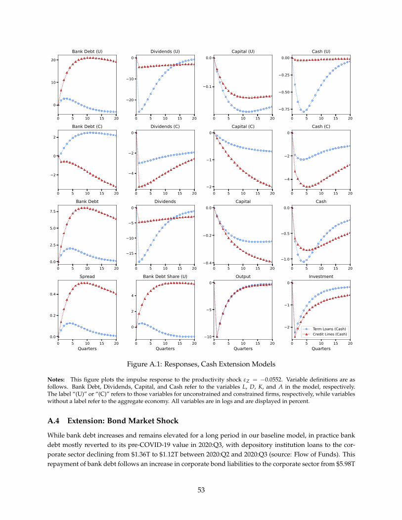
0 5 10 15 20

0

10

20

Bank Debt (U)

0 5 10 15 20

20

10

0Dividends (U)

0 5 10 15 20

0.1

0.0Capital (U)

0 5 10 15 20

0.75

0.50

0.25

0.00Cash (U)

0 5 10 15 20

2

0

2

Bank Debt (C)

0 5 10 15 20

4

2

0Dividends (C)

0 5 10 15 202

1

0Capital (C)

0 5 10 15 20

4

2

0Cash (C)

0 5 10 15 200.0

2.5

5.0

7.5

Bank Debt

0 5 10 15 20

15

10

5

0Dividends

0 5 10 15 200.4

0.2

0.0Capital

0 5 10 15 20

1.0

0.5

0.0Cash

0 5 10 15 20Quarters

0.0

0.2

0.4

Spread

0 5 10 15 20Quarters

0

2

4

Bank Debt Share (U)

0 5 10 15 20Quarters

10

5

0Output

0 5 10 15 20Quarters

2

1

0Investment

Term Loans (Cash)Credit Lines (Cash)

Figure A.1: Responses, Cash Extension Models

Notes: This figure plots the impulse response to the productivity shock εZ = −0.0552. Variable definitions are asfollows. Bank Debt, Dividends, Capital, and Cash refer to the variables L, D, K, and A in the model, respectively.The label “(U)” or “(C)” refers to those variables for unconstrained and constrained firms, respectively, while variableswithout a label refer to the aggregate economy. All variables are in logs and are displayed in percent.

A.4 Extension: Bond Market Shock

While bank debt increases and remains elevated for a long period in our baseline model, in practice bankdebt mostly reverted to its pre-COVID-19 value in 2020:Q3, with depository institution loans to the cor-porate sector declining from $1.36T to $1.12T between 2020:Q2 and 2020:Q3 (source: Flow of Funds). Thisrepayment of bank debt follows an increase in corporate bond liabilities to the corporate sector from $5.98T

53

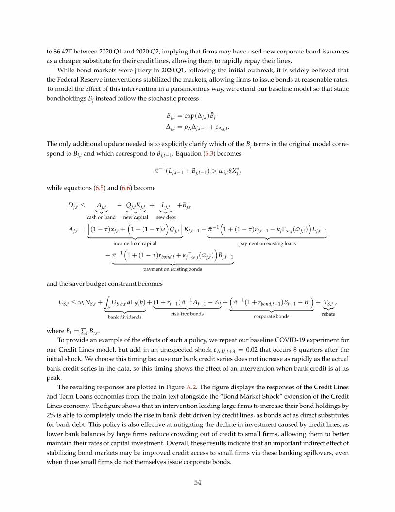
to $6.42T between 2020:Q1 and 2020:Q2, implying that firms may have used new corporate bond issuancesas a cheaper substitute for their credit lines, allowing them to rapidly repay their lines.

While bond markets were jittery in 2020:Q1, following the initial outbreak, it is widely believed thatthe Federal Reserve interventions stabilized the markets, allowing firms to issue bonds at reasonable rates.To model the effect of this intervention in a parsimonious way, we extend our baseline model so that staticbondholdings Bj instead follow the stochastic process

Bj,t = exp(∆j,t)Bj

∆j,t = ρ∆∆j,t−1 + ε∆,j,t.

The only additional update needed is to explicitly clarify which of the Bj terms in the original model corre-spond to Bj,t and which correspond to Bj,t−1. Equation (6.3) becomes

π−1(Lj,t−1 + Bj,t−1) > ωi,tθX∗j,t

while equations (6.5) and (6.6) become

Dj,t ≤ Aj,t︸︷︷︸cash on hand

− Qj,tKj,t︸ ︷︷ ︸new capital

+ Lj,t︸︷︷︸new debt

+Bj,t

Aj,t =[(1− τ)xj,t +

(1− (1− τ)δ

)Qj,t

]︸ ︷︷ ︸

income from capital

Kj,t−1 − π−1(

1 + (1− τ)rj,t−1 + κjΓω,j(ωj,t))

Lj,t−1︸ ︷︷ ︸payment on existing loans

− π−1(

1 + (1− τ)rbond,t + κjΓω,j(ωj,t))

Bj,t−1︸ ︷︷ ︸payment on existing bonds

and the saver budget constraint becomes

CS,t ≤ wtNS,t +∫

bDS,b,t dΓb(b)︸ ︷︷ ︸

bank dividends

+ (1 + rt−1)π−1 At−1 − At︸ ︷︷ ︸

risk-free bonds

+(

π−1(1 + rbond,t−1)Bt−1 − Bt

)︸ ︷︷ ︸

corporate bonds

+ TS,t︸︷︷︸rebate

,

where Bt = ∑j Bj,t.To provide an example of the effects of such a policy, we repeat our baseline COVID-19 experiment for

our Credit Lines model, but add in an unexpected shock ε∆,U,t+8 = 0.02 that occurs 8 quarters after theinitial shock. We choose this timing because our bank credit series does not increase as rapidly as the actualbank credit series in the data, so this timing shows the effect of an intervention when bank credit is at itspeak.

The resulting responses are plotted in Figure A.2. The figure displays the responses of the Credit Linesand Term Loans economies from the main text alongside the “Bond Market Shock” extension of the CreditLines economy. The figure shows that an intervention leading large firms to increase their bond holdings by2% is able to completely undo the rise in bank debt driven by credit lines, as bonds act as direct substitutesfor bank debt. This policy is also effective at mitigating the decline in investment caused by credit lines, aslower bank balances by large firms reduce crowding out of credit to small firms, allowing them to bettermaintain their rates of capital investment. Overall, these results indicate that an important indirect effect ofstabilizing bond markets may be improved credit access to small firms via these banking spillovers, evenwhen those small firms do not themselves issue corporate bonds.

54

0 5 10 15 20

0

10

20

Bank Debt (U)

0 5 10 15 200.2

0.1

0.0Capital (U)

0 5 10 15 20

30

20

10

0Dividends (U)

0 5 10 15 20

5

0

Bank Debt (C)

0 5 10 15 20

3

2

1

0Capital (C)

0 5 10 15 2010

5

0Dividends (C)

0 5 10 15 2010

5

0Output

0 5 10 15 200.6

0.4

0.2

0.0Capital

0 5 10 15 20

20

10

0Dividends

0 5 10 15 20Quarters

0

2

4

6

Bank Debt

0 5 10 15 20Quarters

0.0

0.5

1.0

Spread

0 5 10 15 20Quarters

0.0

2.5

5.0

Bank Debt Share (U)

Credit LinesBond Market ShockTerm Loans

Figure A.2: Responses, Baseline Experiment vs. Bond Market Shock

Notes: The “Bond Market Shock” plots the impulse response to the productivity shock εZ = −0.0552 at time 0 in theCredit Lines economy, followed by the bond market shock ε∆,U,t = 0.02 at time 8. The Credit Lines and Term Loanseconomies are defined as in Section 6.5. Variable definitions are as follows: “Debt (U)” is LU,t; “Capital (U)” is KU,t;“Dividends (U)” is DU,t; “Debt (C)” is LC,t; “Capital (C)” is KC,t; “Dividends (C)” is DC,t; “Output” is Yt; “Capital” isaUKU,t + aCKC,t; “Dividends” is aU DU,t + aCDC,t; “Debt” is aU LU,t + aC LC,t; “Spread” is sC,t, equivalently sU,t in theAll Unconstrained and Term Loans economies; “Debt Share (U)” is aU LU,t/(aU LU,t + aC LC,t). All variables except for“Spread” and “Debt Share (U)” are in logs, and all variables are displayed in percent.

At the same time, the capital stock still remains depressed following the intervention relative to theTerm Loans economy. While total bank debt returns to roughly its steady state level following the interven-

55

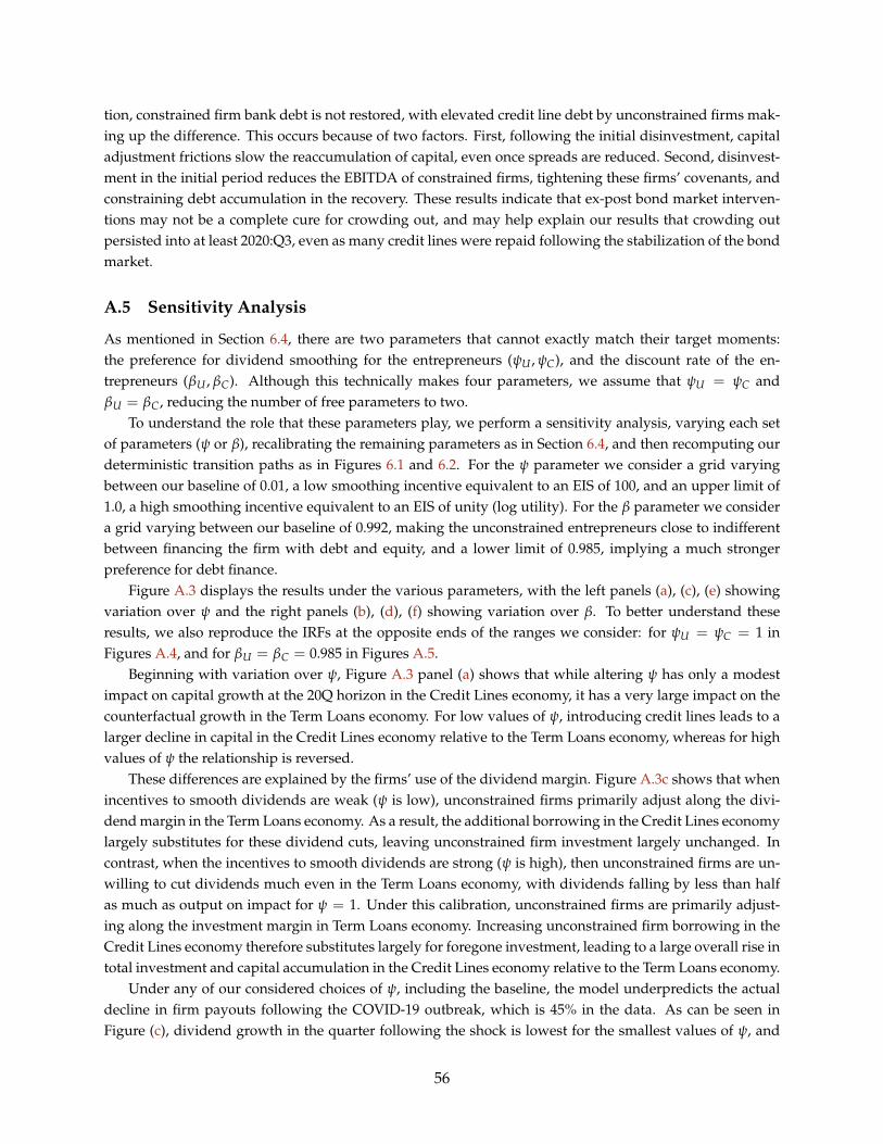
tion, constrained firm bank debt is not restored, with elevated credit line debt by unconstrained firms mak-ing up the difference. This occurs because of two factors. First, following the initial disinvestment, capitaladjustment frictions slow the reaccumulation of capital, even once spreads are reduced. Second, disinvest-ment in the initial period reduces the EBITDA of constrained firms, tightening these firms’ covenants, andconstraining debt accumulation in the recovery. These results indicate that ex-post bond market interven-tions may not be a complete cure for crowding out, and may help explain our results that crowding outpersisted into at least 2020:Q3, even as many credit lines were repaid following the stabilization of the bondmarket.

A.5 Sensitivity Analysis

As mentioned in Section 6.4, there are two parameters that cannot exactly match their target moments:the preference for dividend smoothing for the entrepreneurs (ψU , ψC), and the discount rate of the en-trepreneurs (βU , βC). Although this technically makes four parameters, we assume that ψU = ψC andβU = βC, reducing the number of free parameters to two.

To understand the role that these parameters play, we perform a sensitivity analysis, varying each setof parameters (ψ or β), recalibrating the remaining parameters as in Section 6.4, and then recomputing ourdeterministic transition paths as in Figures 6.1 and 6.2. For the ψ parameter we consider a grid varyingbetween our baseline of 0.01, a low smoothing incentive equivalent to an EIS of 100, and an upper limit of1.0, a high smoothing incentive equivalent to an EIS of unity (log utility). For the β parameter we considera grid varying between our baseline of 0.992, making the unconstrained entrepreneurs close to indifferentbetween financing the firm with debt and equity, and a lower limit of 0.985, implying a much strongerpreference for debt finance.

Figure A.3 displays the results under the various parameters, with the left panels (a), (c), (e) showingvariation over ψ and the right panels (b), (d), (f) showing variation over β. To better understand theseresults, we also reproduce the IRFs at the opposite ends of the ranges we consider: for ψU = ψC = 1 inFigures A.4, and for βU = βC = 0.985 in Figures A.5.

Beginning with variation over ψ, Figure A.3 panel (a) shows that while altering ψ has only a modestimpact on capital growth at the 20Q horizon in the Credit Lines economy, it has a very large impact on thecounterfactual growth in the Term Loans economy. For low values of ψ, introducing credit lines leads to alarger decline in capital in the Credit Lines economy relative to the Term Loans economy, whereas for highvalues of ψ the relationship is reversed.

These differences are explained by the firms’ use of the dividend margin. Figure A.3c shows that whenincentives to smooth dividends are weak (ψ is low), unconstrained firms primarily adjust along the divi-dend margin in the Term Loans economy. As a result, the additional borrowing in the Credit Lines economylargely substitutes for these dividend cuts, leaving unconstrained firm investment largely unchanged. Incontrast, when the incentives to smooth dividends are strong (ψ is high), then unconstrained firms are un-willing to cut dividends much even in the Term Loans economy, with dividends falling by less than halfas much as output on impact for ψ = 1. Under this calibration, unconstrained firms are primarily adjust-ing along the investment margin in Term Loans economy. Increasing unconstrained firm borrowing in theCredit Lines economy therefore substitutes largely for foregone investment, leading to a large overall rise intotal investment and capital accumulation in the Credit Lines economy relative to the Term Loans economy.

Under any of our considered choices of ψ, including the baseline, the model underpredicts the actualdecline in firm payouts following the COVID-19 outbreak, which is 45% in the data. As can be seen inFigure (c), dividend growth in the quarter following the shock is lowest for the smallest values of ψ, and

56

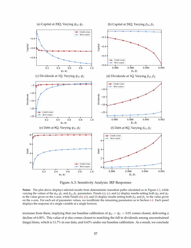
(a) Capital at 20Q, Varying ψU , ψC

0.2 0.4 0.6 0.8 1.0U, C

0.8

0.6

0.4

Capi

tal

Credit LinesTerm Loans

(b) Capital at 20Q, Varying βU , βC

0.986 0.988 0.990 0.992U, C

0.6

0.5

0.4

0.3

Capi

tal

Credit LinesTerm Loans

(c) Dividends at 1Q, Varying ψU , ψC

0.2 0.4 0.6 0.8 1.0U, C

25

20

15

10

5

Divi

dend

s

Credit LinesTerm Loans

(d) Dividends at 1Q, Varying βU , βC

0.986 0.988 0.990 0.992U, C

25

20

15

10

Divi

dend

s

Credit LinesTerm Loans

(e) Debt at 8Q, Varying ψU , ψC

0.2 0.4 0.6 0.8 1.0U, C

2

4

6

8

Debt

Credit LinesTerm Loans

(f) Debt at 8Q, Varying βU , βC

0.986 0.988 0.990 0.992U, C

0

2

4

6

Debt

Credit LinesTerm Loans

Figure A.3: Sensitivity Analysis: IRF Responses

Notes: The plot above displays selected results from deterministic transition paths calculated as in Figure 6.2, whilevarying the values of the ψU , ψC and βU , βC parameters. Panels (a), (c), and (e) display results setting both ψU and ψCto the value given on the x-axis, while Panels (b), (d), and (f) display results setting both βU and βC to the value givenon the x-axis. For each set of parameter values, we recalibrate the remaining parameters as in Section 6.4. Each paneldisplays the response of a single variable at a single horizon.

increases from there, implying that our baseline calibration of ψU = ψC = 0.01 comes closest, delivering adecline of 6.00%. This value of ψ also comes closest to matching the fall in dividends among unconstrained(large) firms, which is 11.7% in our data, and 4.63% under our baseline calibration. As a result, we conclude

57

that our calibration with the most flexible dividend margin (lowest ψ) comes closest to fitting the data.Beyond moment matching, a more general justification comes from a broader look at corporate finance.

Although we refer to firm payouts as “dividends” in our model, this margin really reflects any financialtransactions firms could use to avoid reducing either bank debt or investment. For example, while firmsseem to make efforts to keep quarterly dividends smooth, they distribute a comparable amount of payoutsin the form of repurchases, the size of which is both volatile and irregular. Firms that utilize repurchasesshould therefore be able to adjust their payouts very flexibly. Adjustments to nonbank credit or cash wouldsimilarly be reflected by this margin. Such transactions, potentially carry a small but nontrivial cost interms of fees, flexibility, or potential negative signals to the market, are an alternative interpretation of thedividend margin in our model, and point to a low but nonzero value for ψ.

Next, we can consider variation over β. Panel (b) shows that as the calibrated value for βU and βC

decreases, the difference in capital accumulation between the Credit Lines and Term Loans economies atthe 20Q horizon falls sharply. The mechanism behind this result is a bit subtle, and largely occurs throughindirect effects on how other parameters are internally calibrated. Recall that the violation cost κj is cali-brated to match the leverage ratio of each type of firm in the data. When βU falls, the value of borrowingfrom the entrepreneurs’ perspective rises, and so the model must calibrate a higher violation cost κU tokeep unconstrained leverage at the target level. With higher violation costs, unconstrained firms’ capitalstructure decisions are effectively driven more by the marginal cost of increased violation costs ξU,t and lessby the direct cost of credit rj,t. Because of this, introducing credit lines have a much smaller impact on firmborrowing, since their main benefit (lower rates) are less important in a model where lending is primarilydriven by covenant concerns.

This mechanism implies that aggregate borrowing, shown at the 8Q horizon in Panel (f), is stronglyincreasing in βU in the Credit Lines economy. Since our model underpredicts the actual growth of bank-firm debt, which was 23.7% larger in 2020:Q1 than in 2019:Q4, we come closest by choosing a value of βU

as high as possible, yielding a peak increase in bank-firm credit of around 7%. This calibration impliesthat unconstrained firms are close to indifferent between financing with bank debt or internally in steadystate, which we believe is reasonable considering that firms have access to many forms of nonbank creditin practice.

58

0 5 10 15 200

10

20

Bank Debt (U)

0 5 10 15 20

0.75

0.50

0.25

0.00Capital (U)

0 5 10 15 20

3

2

1

0Dividends (U)

0 5 10 15 20

5

0

Bank Debt (C)

0 5 10 15 204

2

0Capital (C)

0 5 10 15 2010

5

0Dividends (C)

0 5 10 15 2010

5

0Output

0 5 10 15 20

0.5

0.0Capital

0 5 10 15 20

4

2

0Dividends

0 5 10 15 20Quarters

0.0

2.5

5.0

7.5

Bank Debt

0 5 10 15 20Quarters

0.0

0.5

1.0Spread

0 5 10 15 20Quarters

0.0

2.5

5.0

7.5

Bank Debt Share (U)Credit LinesTerm Loans

Figure A.4: Responses: Credit Line vs. Term Loan Economies, ψU = ψC = 1

Notes: This figure plots the impulse response to the productivity shock εZ = −0.0552. Variable definitions areas follows: “Debt (U)” is LU,t; “Capital (U)” is KU,t; “Dividends (U)” is DU,t; “Debt (C)” is LC,t; “Capital (C)” isKC,t; “Dividends (C)” is DC,t; “Output” is Yt; “Capital” is aUKU,t + aCKC,t; “Dividends” is aU DU,t + aCDC,t; “Debt” isaU LU,t + aC LC,t; “Spread” is sC,t, equivalently sU,t in the All Unconstrained and Term Loans economies; “Debt Share(U)” is aU LU,t/(aU LU,t + aC LC,t). All variables except for “Spread” and “Debt Share (U)” are in logs, and all variablesare displayed in percent.

59

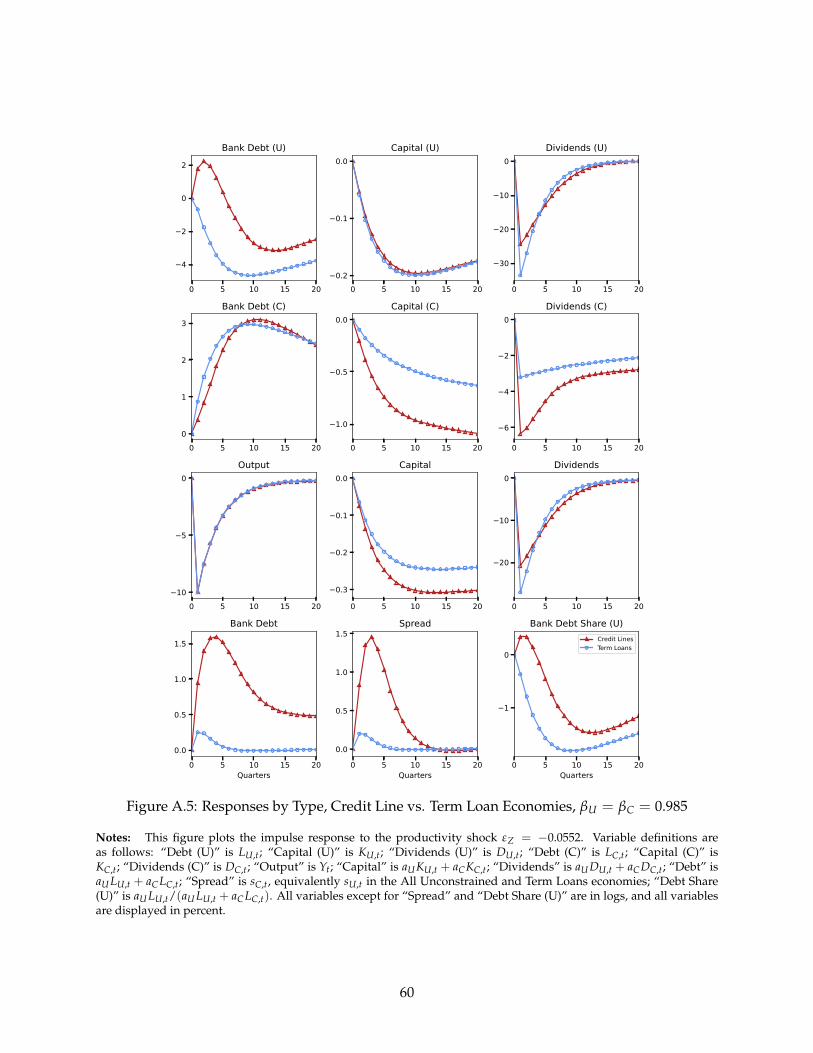
0 5 10 15 20

4

2

0

2

Bank Debt (U)

0 5 10 15 200.2

0.1

0.0Capital (U)

0 5 10 15 20

30

20

10

0Dividends (U)

0 5 10 15 200

1

2

3

Bank Debt (C)

0 5 10 15 20

1.0

0.5

0.0Capital (C)

0 5 10 15 20

6

4

2

0Dividends (C)

0 5 10 15 2010

5

0Output

0 5 10 15 20

0.3

0.2

0.1

0.0Capital

0 5 10 15 20

20

10

0Dividends

0 5 10 15 20Quarters

0.0

0.5

1.0

1.5

Bank Debt

0 5 10 15 20Quarters

0.0

0.5

1.0

1.5Spread

0 5 10 15 20Quarters

1

0

Bank Debt Share (U)Credit LinesTerm Loans

Figure A.5: Responses by Type, Credit Line vs. Term Loan Economies, βU = βC = 0.985

Notes: This figure plots the impulse response to the productivity shock εZ = −0.0552. Variable definitions areas follows: “Debt (U)” is LU,t; “Capital (U)” is KU,t; “Dividends (U)” is DU,t; “Debt (C)” is LC,t; “Capital (C)” isKC,t; “Dividends (C)” is DC,t; “Output” is Yt; “Capital” is aUKU,t + aCKC,t; “Dividends” is aU DU,t + aCDC,t; “Debt” isaU LU,t + aC LC,t; “Spread” is sC,t, equivalently sU,t in the All Unconstrained and Term Loans economies; “Debt Share(U)” is aU LU,t/(aU LU,t + aC LC,t). All variables except for “Spread” and “Debt Share (U)” are in logs, and all variablesare displayed in percent.

60

B Aggregate Responses to Monetary Policy Shocks

B.1 Further Evidence and Robustness

In this Appendix, we describe the estimations of the impulse responses in Figure 1.1 and provide furtherevidence and robustness checks. Given an identified series of monetary policy shocks, we run several localprojections. Let yt be the outcome variable at time t, e.g., (log) real credit or the federal funds rate. FollowingJordà (2005), we estimate

yt+h − yt−1 = αh + βh · εMPt + γhXt−1 + uh

t , (B.1)

where h = 0, 1, ..., 48. The estimated coefficients βh give the percentage (point) change at horizon h to a100-basis-point monetary policy shock εMP

t . Xt−1 denotes a vector of controls. The specification in Figure1.1 includes one year of lagged values of the monetary policy shock and one year of lagged values of theone-month change in the respective dependent variable. We check and confirm the robustness of the resultsto the choice of the lag length, as explained below.

Figure B.1 replicates the results in Figure 1.1 and additionally shows the responses for the “FederalFunds Rate,” “Industrial Production,” “Consumer Price Index,” “Deposits,” “Loans & Leases,” and “Secu-rities.”54 Importantly, in response to a monetary policy tightening, deposits flow out of the banking sector(Drechsler et al., 2017), in contrast to the behavior of deposits around the outbreak of COVID-19 (see Figure1.2). This deposit outflow may be an additional source of bank credit supply contraction after a monetarypolicy tightening.

In Figures B.2-B.4, we provide further evidence. First, we test whether the findings depend on thechoice of the lag length. Figure B.2 shows that the results remain much the same whether any, one year, ortwo years worth of controls of the shocks and the one-month change in the dependent variable are added.Second, we check whether the responses depend on the identification approach. Using the high-frequencyidentification approach (see e.g., Gürkaynak et al., 2005), Figure B.3 shows impulse responses to the shockseries from Nakamura and Steinsson (2018) for the sample 1994:M1 - 2007:M12.55 Apart from the CPIresponse, which shows a price puzzle initially, the remaining responses are similar compared with the onesin Figure 1.1.

Last, we investigate the response of total firm credit using quarterly data from the Flow of Funds (seeAppendix Table C.1 for details about the data). Figure B.4 shows the impulse responses of various types ofcredit to nonfinancial businesses following a contractionary monetary policy shock.56 Nonfinancial busi-nesses can be separated into corporate and noncorporate categories. Nonfinancial noncorporate businesses(e.g., sole proprietorships and limited partnerships) only borrow using loans, and panel (b) shows that suchcredit contracts to a monetary policy tightening. These loans likely consist of term loans, so this responseis consistent with the results in Section 5.1. In contrast, corporate loans, which include more credit lines,increase as shown in panel (c), again in line with the findings in Section 5.1. In addition, corporate debt

54We do not include controls in the equation for the federal funds rate, since the rate responds on impact to theshock. The responses of the federal funds rate are largely unaffected by including additional controls.

55The policy news shock series by Nakamura and Steinsson (2018) is the first principal component across surprisechanges of five futures contracts around scheduled policy announcements: the one with respect to the Fed funds rateimmediately following a meeting by the Federal Open Market Committee (FOMC), the expected federal funds rateimmediately following the next FOMC meeting, and expected three-month eurodollar interest rates at horizons of two,three, and four quarters. These are the same contracts that are used in the rotations by Gürkaynak et al. (2005). Thescale of the shock series is arbitrary, and we rescale it such that its effect on the two-year government bond yield is oneand therefore comparable to the results in Section 5.1.

56All local projections include one year of lagged values of the monetary policy shock and the one-month change inthe respective dependent variable as controls.

61

securities also rise after an initial dip (see panel (d)). Commercial paper and corporate bonds, which areboth part of corporate debt securities, also increase as shown in panels (e) and (f), after a drop over the firstquarters for corporate bonds. Taking all corporate and noncorporate loans and debt securities together,total firm credit also rises following a monetary policy tightening, as shown in panel (a).

Figure B.1: Impulse Responses to a Monetary Policy Shock.

Notes: Impulse responses to a 1 percentage point contractionary monetary policy shock based on the identificationapproach by Romer and Romer (2004). The shock series is taken from Coibion et al. (2017) and the remaining dataare obtained from St. Louis Fed’s FRED database. The credit series are based on the H.8 releases for U.S. commercialbanks from the Board of Governors of the Federal Reserve (see Appendix Table C.1 for details about the data). Sample:1970:M1 - 2007:M12. 95 and 68 percent confidence bands are shown using Newey and West (1987) standard errors.

62

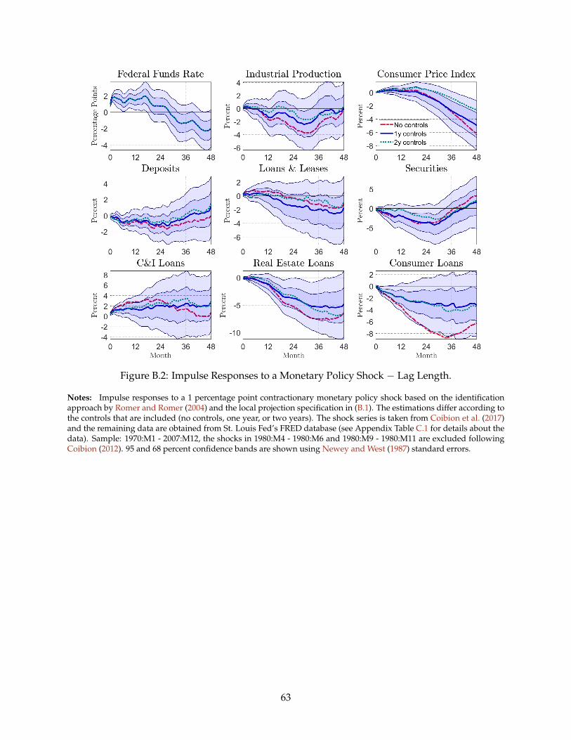
Figure B.2: Impulse Responses to a Monetary Policy Shock − Lag Length.

Notes: Impulse responses to a 1 percentage point contractionary monetary policy shock based on the identificationapproach by Romer and Romer (2004) and the local projection specification in (B.1). The estimations differ according tothe controls that are included (no controls, one year, or two years). The shock series is taken from Coibion et al. (2017)and the remaining data are obtained from St. Louis Fed’s FRED database (see Appendix Table C.1 for details about thedata). Sample: 1970:M1 - 2007:M12, the shocks in 1980:M4 - 1980:M6 and 1980:M9 - 1980:M11 are excluded followingCoibion (2012). 95 and 68 percent confidence bands are shown using Newey and West (1987) standard errors.

63

Figure B.3: Impulse Responses to a Monetary Policy Shock − High-Frequency Surprises.

Notes: Impulse responses to a 1 percentage point contractionary monetary policy shock based on the local projectionspecification in (B.1). The shock series follows the computations in Nakamura and Steinsson (2018) (see also footnote55) and the remaining series are obtained from St. Louis Fed’s FRED database (see Appendix Table C.1 for details aboutthe data). All specifications exclude additional controls, apart from the estimations for industrial production and theconsumer price index, for which two years worth of the shocks and the one-month change in the respective dependentvariable are included. Sample: 1994:M1 - 2007:M12. 95 and 68 percent confidence bands are shown using Newey andWest (1987) standard errors.

64

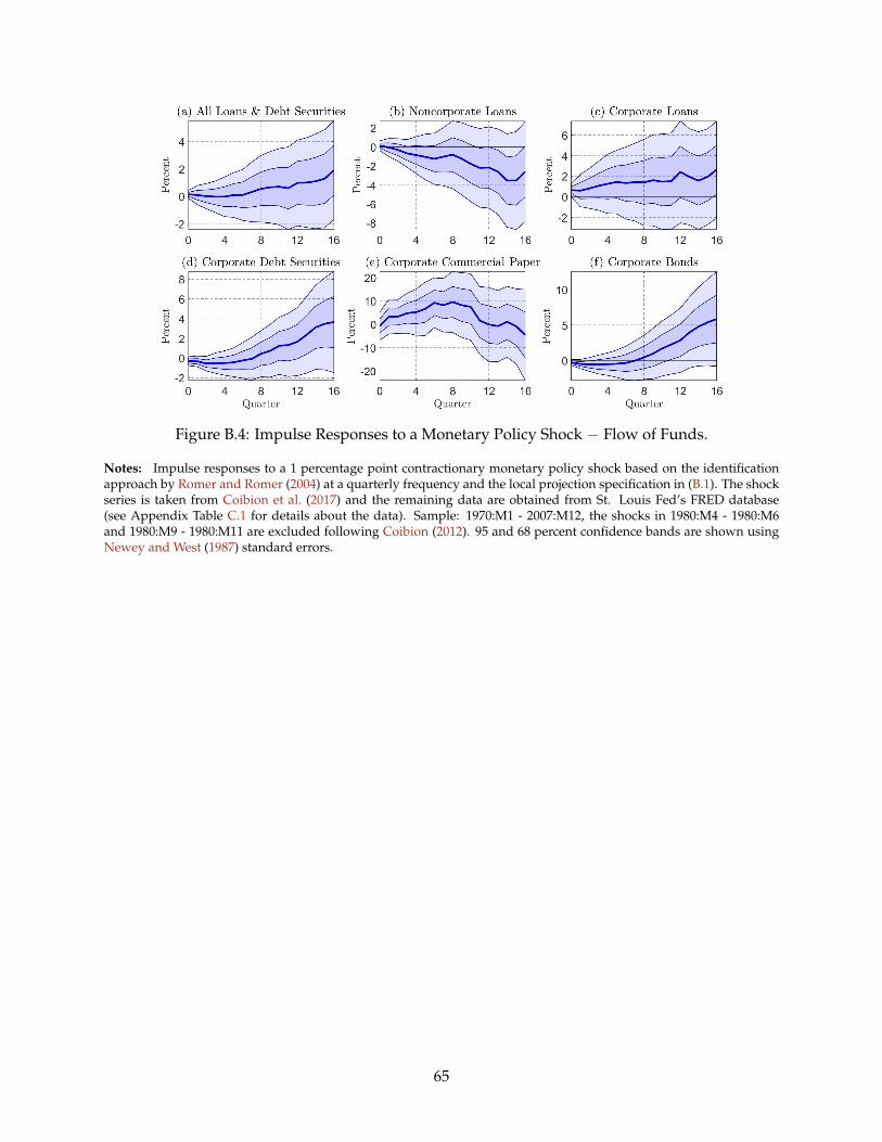
Figure B.4: Impulse Responses to a Monetary Policy Shock − Flow of Funds.

Notes: Impulse responses to a 1 percentage point contractionary monetary policy shock based on the identificationapproach by Romer and Romer (2004) at a quarterly frequency and the local projection specification in (B.1). The shockseries is taken from Coibion et al. (2017) and the remaining data are obtained from St. Louis Fed’s FRED database(see Appendix Table C.1 for details about the data). Sample: 1970:M1 - 2007:M12, the shocks in 1980:M4 - 1980:M6and 1980:M9 - 1980:M11 are excluded following Coibion (2012). 95 and 68 percent confidence bands are shown usingNewey and West (1987) standard errors.

65

C Data

C.1 Variable Definitions and Data Sources

In Tables C.1-C.5, we provide names, definitions, and sources for all variables that are used in the empiricalanalysis. Table C.1 reports the macro time series that are used in Section 1 and Appendix B. Table C.2collects all variables that are used from the FR Y-14Q H.1 data, Table C.3 the ones from Compustat, andTable C.4 reports the ones from Orbis. These variables are employed in Sections 3-5 and the Appendix. Thevariables from the FR Y-9C Filings are described in Table C.5.

Table C.1: Macro Time Series.

Variable Name Description SourceBank Credit H.8 releases, All U.S. commercial banks, weekly, SA FREDLoans and Leases H.8 releases, All U.S. commercial banks, weekly, SA FREDSecurities H.8 releases, All U.S. commercial banks, weekly, SA FREDC&I Loans H.8 releases, All U.S. commercial banks, weekly, SA FREDReal Estate Loans H.8 releases, All U.S. commercial banks, weekly, SA FREDConsumer Loans H.8 releases, All U.S. commercial banks, weekly, SA FREDTotal Assets H.8 releases, All U.S. commercial banks, weekly, SA FREDDeposits H.8 releases, All U.S. commercial banks, weekly, SA FREDFederal Funds Rate Effective funds rate, daily, NSA FREDConsumer Price Index All Items for the United States, SA, 2015=100 FREDIndustrial Production Real Index, 2012=100, SA FREDGross Domestic Product Real, Billions of Chained 2012 Dollars, SA FREDGilchrist-Zakrajsek Spread Based on Gilchrist and Zakrajšek (2012), NSA FEDS NotesNonfinancial Business;

Flow of Funds, NSA FREDDebt Securities and LoansNonfinancial Noncorporate

Flow of Funds, NSA FREDBusiness; LoansNonfinancial Corporate

Flow of Funds, NSA FREDBusiness; LoansNonfinancial Corporate

Flow of Funds, NSA FREDBusiness; Debt SecuritiesNonfinancial Corporate

Flow of Funds, NSA FREDBusiness; Commercial PaperNonfinancial Corporate

Flow of Funds, NSA FREDBusiness; Corporate Bonds

Notes: All nominal credit series are converted into real series using the consumer price index. All weekly or monthlytime series are averaged to monthly or quarterly frequency for purposes of computing impulse responses in Figure1.1 and Appendix B. Notation: “FRED” = St. Louis Fed’s FRED Database, ”SA” = seasonally-adjusted, “NSA” = non-seasonally-adjusted.

66

Table C.2: FR Y-14 Variable Definitions.

Variable Name Description / Use Field No.Zip code Zip code of headquarters 7Industry Derived 2-Digit NAICS Code 8Internal risk rating Internal risk rating mapped to S&P scale 10TIN Taxpayer Identification Number 11Internal Credit Facility ID Used together with BHC and previous facility ID to

construct loan histories15

Previous Internal CreditFacility ID

Used together with BHC and facility ID to construct loanhistories

16

Origination Date Used to distinguish new and existing loans 18Maturity Date Used to determine remaining maturity 19Term Loan Loan facility type reported as Term Loan, includes Term

Loan A-C, Bridge Loans, Asset-Based, and Debtor inPossession.

20

Credit Line Loan facility type reported as revolving or non-revolvingline of credit, standby letter of credit, fronting exposure,or commitment to commit.

20

Purpose Credit facility purpose 22Committed Credit Committed credit exposure 24Used Credit Utilized credit exposure 25Line Reported on Y-9C Line number reported in HC-C schedule of FR Y-9C 26Secured Credit Security type of credit 36Variable Rate Interest rate variability reported as “Floating” or “Mixed” 37Interest Rate Current interest rate 38Date Financials Financial statement date used to match firm financials to

Y-14 date52

EBITDA Derived from operating income plus depreciation andamortization

56, 57

Interest Expense Used in calculating implied covenants 58Net Income Current and prior year net income for trailing 12-months

used to construct cash flow changes59, 60

Cash and Securities Cash and marketable securities 61Tangible Assets Tangible assets 68Total Assets Total assets, current year and prior year 70Short Term Debt Used in calculating implied covenants & total debt 74Long Term Debt Used in calculating implied covenants & total debt 78Total Liabilities Total liabilities 80Capital Expenditures 12-month trailing CAPEX 82Probability of Default Probability of default for firms 88Collateral Value Collateral market value 93Syndicated Loan Syndicated loan flag 100

Notes: All nominal series are converted into real series using the consumer price index (see TableC.1). The corresponding “Field No.” can be found in the data dictionary (Schedule H.1, pp. 162-217):https://www.federalreserve.gov/reportforms/forms/FR_Y-14Q20200331_i.pdf

67

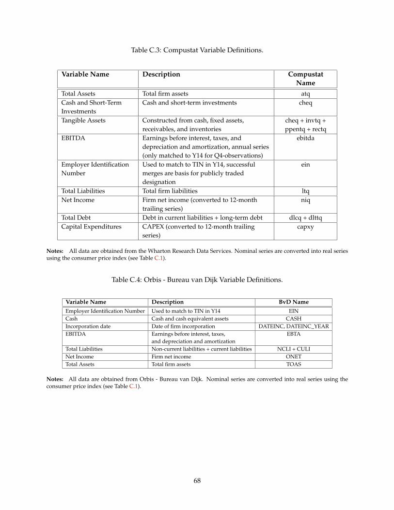
Table C.3: Compustat Variable Definitions.

Variable Name Description CompustatName

Total Assets Total firm assets atqCash and Short-TermInvestments

Cash and short-term investments cheq

Tangible Assets Constructed from cash, fixed assets,receivables, and inventories

cheq + invtq +ppentq + rectq

EBITDA Earnings before interest, taxes, anddepreciation and amortization, annual series(only matched to Y14 for Q4-observations)

ebitda

Employer IdentificationNumber

Used to match to TIN in Y14, successfulmerges are basis for publicly tradeddesignation

ein

Total Liabilities Total firm liabilities ltqNet Income Firm net income (converted to 12-month

trailing series)niq

Total Debt Debt in current liabilities + long-term debt dlcq + dlttqCapital Expenditures CAPEX (converted to 12-month trailing

series)capxy

Notes: All data are obtained from the Wharton Research Data Services. Nominal series are converted into real seriesusing the consumer price index (see Table C.1).

Table C.4: Orbis - Bureau van Dijk Variable Definitions.

Variable Name Description BvD NameEmployer Identification Number Used to match to TIN in Y14 EINCash Cash and cash equivalent assets CASHIncorporation date Date of firm incorporation DATEINC, DATEINC_YEAREBITDA Earnings before interest, taxes, EBTA

and depreciation and amortizationTotal Liabilities Non-current liabilities + current liabilities NCLI + CULINet Income Firm net income ONETTotal Assets Total firm assets TOAS

Notes: All data are obtained from Orbis - Bureau van Dijk. Nominal series are converted into real series using theconsumer price index (see Table C.1).

68

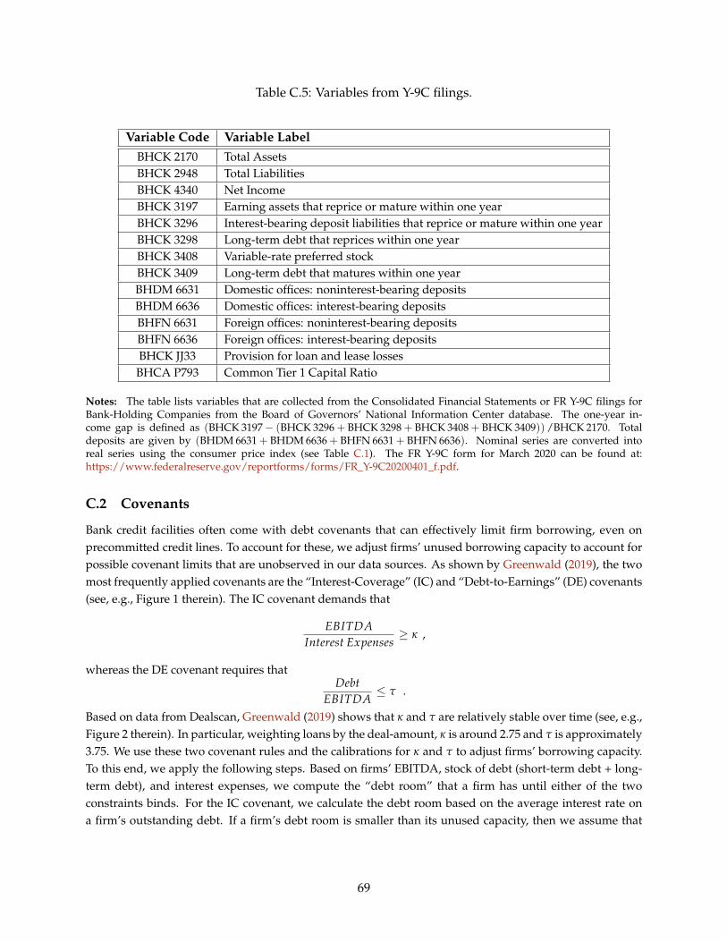
Table C.5: Variables from Y-9C filings.

Variable Code Variable LabelBHCK 2170 Total AssetsBHCK 2948 Total LiabilitiesBHCK 4340 Net IncomeBHCK 3197 Earning assets that reprice or mature within one yearBHCK 3296 Interest-bearing deposit liabilities that reprice or mature within one yearBHCK 3298 Long-term debt that reprices within one yearBHCK 3408 Variable-rate preferred stockBHCK 3409 Long-term debt that matures within one yearBHDM 6631 Domestic offices: noninterest-bearing depositsBHDM 6636 Domestic offices: interest-bearing depositsBHFN 6631 Foreign offices: noninterest-bearing depositsBHFN 6636 Foreign offices: interest-bearing depositsBHCK JJ33 Provision for loan and lease lossesBHCA P793 Common Tier 1 Capital Ratio

Notes: The table lists variables that are collected from the Consolidated Financial Statements or FR Y-9C filings forBank-Holding Companies from the Board of Governors’ National Information Center database. The one-year in-come gap is defined as (BHCK 3197− (BHCK 3296 + BHCK 3298 + BHCK 3408 + BHCK 3409)) /BHCK 2170. Totaldeposits are given by (BHDM 6631 + BHDM 6636 + BHFN 6631 + BHFN 6636). Nominal series are converted intoreal series using the consumer price index (see Table C.1). The FR Y-9C form for March 2020 can be found at:https://www.federalreserve.gov/reportforms/forms/FR_Y-9C20200401_f.pdf.

C.2 Covenants

Bank credit facilities often come with debt covenants that can effectively limit firm borrowing, even onprecommitted credit lines. To account for these, we adjust firms’ unused borrowing capacity to account forpossible covenant limits that are unobserved in our data sources. As shown by Greenwald (2019), the twomost frequently applied covenants are the “Interest-Coverage” (IC) and “Debt-to-Earnings” (DE) covenants(see, e.g., Figure 1 therein). The IC covenant demands that

EBITDAInterest Expenses

≥ κ ,

whereas the DE covenant requires thatDebt

EBITDA≤ τ .

Based on data from Dealscan, Greenwald (2019) shows that κ and τ are relatively stable over time (see, e.g.,Figure 2 therein). In particular, weighting loans by the deal-amount, κ is around 2.75 and τ is approximately3.75. We use these two covenant rules and the calibrations for κ and τ to adjust firms’ borrowing capacity.To this end, we apply the following steps. Based on firms’ EBITDA, stock of debt (short-term debt + long-term debt), and interest expenses, we compute the “debt room” that a firm has until either of the twoconstraints binds. For the IC covenant, we calculate the debt room based on the average interest rate ona firm’s outstanding debt. If a firm’s debt room is smaller than its unused capacity, then we assume that

69

a firm’s actual unused capacity is equal to the debt room.57 Based on this procedure, we find that around37 percent of firms violate one of the two constraints in normal times (2012:Q3-2019:Q4). Chodorow-Reichand Falato (2021) find a slightly lower share of violations across loans (around 25 percent). Hence, while inthe same range, our procedure can be viewed as conservative, since firms with looser limits or without thetype of covenants that we assume could in fact be non-violaters.

C.3 Data Cleaning and Sample Restrictions

We apply the following set of sample restrictions to the Y14 data:

1. We restrict the sample to begin in 2012:Q3. The Y14 collection began in 2011:Q3, but there was asignificant expansion in the number of BHCs required to submit Y14 commercial loan data until2012:Q3. Moreover, the starting date in 2012:Q3 also affords a short phase-in period for the structureof the collection and variables to stabilize.

2. We constrain the sample to loan facilities with line reported on the HC-C schedule in the FR Y9-Cfilings as commercial and industrial loans, “other” loans, “other” leases, and owner-occupied com-mercial real estate (corresponding to Field No. 26 in the H.1 schedule of the Y14 to be equal to 4, 8,9, or 10; see Table C.2). In addition, we drop all observations with NAICS codes 52 and 53 (loans tofinancial firms and real estate firms).

3. When we use information about the facility type (credit line or term loan) or interest rate variabilitytype (i.e., fixed or floating), we exclude observations for which this information is missing or chang-ing over the facility history.

4. Drop all facility records with origination dates before 1990 and maturities greater than 30 years, tominimize the potential influence of data entry errors.

5. Observations with negative or zero values for committed exposure, negative values for utilized ex-posure, and with committed exposure less than utilized exposure are excluded.

6. When aggregating loans at the firm-level, we exclude observations for which the firm identifier “TIN”is missing. To preserve some of these missing values, we fill in missing TINs from a history wherethe non-missing TIN observations are all the same over a unique facility ID.

7. When using information on firms’ financials in the analysis, we apply a set of filters to ensure thatthe reported information is sensible. We exclude observations (i) if total assets, total liabilities, short-term debt, long-term debt, cash assets, tangible assets, or interest expenses are negative, (ii) if tangibleassets, cash assets, or total liabilities are greater than total assets, and (iii) if total debt (short term +long term) is greater than total liabilities.

8. In parts of the empirical analysis, we differentiate between new and existing loans. In some instances,the reporting banks change the IDs for the same facility over time, which would lead to an incorrectclassification of such loans as newly issued. To address this issue, we use information on whether acredit facility previously had a different ID, which banks have to report in the Y14 (see Table C.2). Ifwe can find a record for the prior ID, we append the history of the new ID onto the history of theprior ID.

57To account for covenant limits in Figure 3.1, we adjust the total amount of unused credit based on the ratio of debtroom to unused credit for firms for which we observe all balance sheet and income information within a period.

70

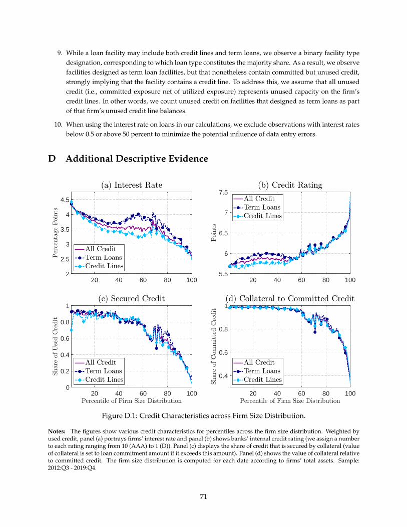
9. While a loan facility may include both credit lines and term loans, we observe a binary facility typedesignation, corresponding to which loan type constitutes the majority share. As a result, we observefacilities designed as term loan facilities, but that nonetheless contain committed but unused credit,strongly implying that the facility contains a credit line. To address this, we assume that all unusedcredit (i.e., committed exposure net of utilized exposure) represents unused capacity on the firm’scredit lines. In other words, we count unused credit on facilities that designed as term loans as partof that firm’s unused credit line balances.

10. When using the interest rate on loans in our calculations, we exclude observations with interest ratesbelow 0.5 or above 50 percent to minimize the potential influence of data entry errors.

D Additional Descriptive Evidence

20 40 60 80 1002

2.5

3

3.5

4

4.5

20 40 60 80 1005.5

6

6.5

7

7.5

20 40 60 80 1000

0.2

0.4

0.6

0.8

1

20 40 60 80 100

0.4

0.6

0.8

1

Figure D.1: Credit Characteristics across Firm Size Distribution.

Notes: The figures show various credit characteristics for percentiles across the firm size distribution. Weighted byused credit, panel (a) portrays firms’ interest rate and panel (b) shows banks’ internal credit rating (we assign a numberto each rating ranging from 10 (AAA) to 1 (D)). Panel (c) displays the share of credit that is secured by collateral (valueof collateral is set to loan commitment amount if it exceeds this amount). Panel (d) shows the value of collateral relativeto committed credit. The firm size distribution is computed for each date according to firms’ total assets. Sample:2012:Q3 - 2019:Q4.

71

20 40 60 80 100

0.4

0.6

0.8

1

20 40 60 80 1000

1

2

3

4

20 40 60 80 1000

0.2

0.4

0.6

0.8

1

20 40 60 80 100

2

4

6

8

20 40 60 80 1000

0.2

0.4

0.6

20 40 60 80 1000

0.2

0.4

0.6

0.8

1

Figure D.2: Credit Characteristics across Firm Size Distribution.

Notes: The figures show various credit characteristics for percentiles across the firm size distribution. The top leftgives the share of loans that carry a variable rate. The top right shows banks’ assessed probability of default. Themiddle left gives the share of used credit that is syndicated and the middle right shows remaining maturity weightedby all used credit. The bottom left gives the share of firms that use at least 90 percent of their committed credit, which isadditionally adjusted for covenants (see Appendix C.2). The bottom right graph shows the average share of observedcredit in our data relative to total debt. The firm size distribution is computed for each date according to firms’ totalassets. Sample: 2012:Q3 - 2019:Q4.

72

20 40 60 80 1000

0.2

0.4

0.6

0.8

1

20 40 60 80 1000

0.2

0.4

0.6

0.8

1

20 40 60 80 1000

0.2

0.4

0.6

0.8

1

20 40 60 80 1000

0.2

0.4

0.6

0.8

1

20 40 60 80 1000

0.2

0.4

0.6

0.8

1

20 40 60 80 1000

0.2

0.4

0.6

0.8

1

Figure D.3: Credit Characteristics across Firm Size Distribution.

Notes: The figures show the share of used credit that is secured by collateral for percentiles across the firm sizedistribution. The top left gives the share of loans that is secured by some type of collateral. The remaining graphsshow the share of used credit secured by real estate (top right), cash and marketable securities (middle left), fixedassets excluding real estate (middle right), accounts receivables and inventory (A.R.I., bottom left), or by a blanket lien(bottom right). The firm size distribution is computed for each date according to firms’ total assets. Sample: 2012:Q3 -2019:Q4.

73

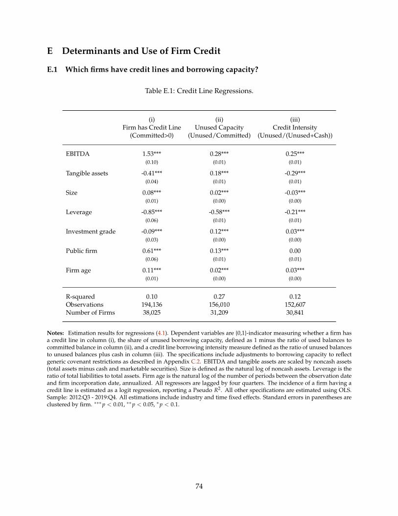
E Determinants and Use of Firm Credit

E.1 Which firms have credit lines and borrowing capacity?

Table E.1: Credit Line Regressions.

(i) (ii) (iii)Firm has Credit Line Unused Capacity Credit Intensity

(Committed>0) (Unused/Committed) (Unused/(Unused+Cash))

EBITDA 1.53*** 0.28*** 0.25***(0.10) (0.01) (0.01)

Tangible assets -0.41*** 0.18*** -0.29***(0.04) (0.01) (0.01)

Size 0.08*** 0.02*** -0.03***(0.01) (0.00) (0.00)

Leverage -0.85*** -0.58*** -0.21***(0.06) (0.01) (0.01)

Investment grade -0.09*** 0.12*** 0.03***(0.03) (0.00) (0.00)

Public firm 0.61*** 0.13*** 0.00(0.06) (0.01) (0.01)

Firm age 0.11*** 0.02*** 0.03***(0.01) (0.00) (0.00)

R-squared 0.10 0.27 0.12Observations 194,136 156,010 152,607Number of Firms 38,025 31,209 30,841

Notes: Estimation results for regressions (4.1). Dependent variables are {0,1}-indicator measuring whether a firm hasa credit line in column (i), the share of unused borrowing capacity, defined as 1 minus the ratio of used balances tocommitted balance in column (ii), and a credit line borrowing intensity measure defined as the ratio of unused balancesto unused balances plus cash in column (iii). The specifications include adjustments to borrowing capacity to reflectgeneric covenant restrictions as described in Appendix C.2. EBITDA and tangible assets are scaled by noncash assets(total assets minus cash and marketable securities). Size is defined as the natural log of noncash assets. Leverage is theratio of total liabilities to total assets. Firm age is the natural log of the number of periods between the observation dateand firm incorporation date, annualized. All regressors are lagged by four quarters. The incidence of a firm having acredit line is estimated as a logit regression, reporting a Pseudo R2. All other specifications are estimated using OLS.Sample: 2012:Q3 - 2019:Q4. All estimations include industry and time fixed effects. Standard errors in parentheses areclustered by firm. ∗∗∗p < 0.01, ∗∗p < 0.05, ∗p < 0.1.

74

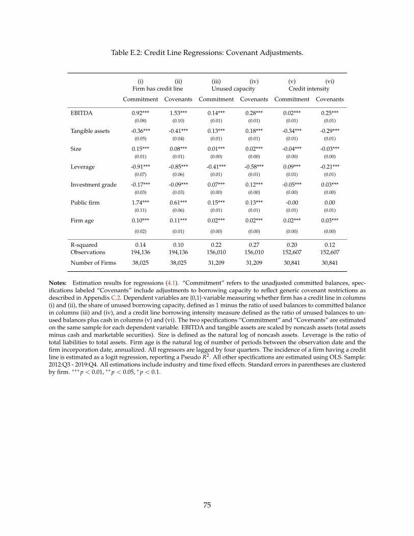
Table E.2: Credit Line Regressions: Covenant Adjustments.

(i) (ii) (iii) (iv) (v) (vi)Firm has credit line Unused capacity Credit intensity

Commitment Covenants Commitment Covenants Commitment Covenants

EBITDA 0.92*** 1.53*** 0.14*** 0.28*** 0.02*** 0.25***(0.08) (0.10) (0.01) (0.01) (0.01) (0.01)

Tangible assets -0.36*** -0.41*** 0.13*** 0.18*** -0.34*** -0.29***(0.05) (0.04) (0.01) (0.01) (0.01) (0.01)

Size 0.15*** 0.08*** 0.01*** 0.02*** -0.04*** -0.03***(0.01) (0.01) (0.00) (0.00) (0.00) (0.00)

Leverage -0.91*** -0.85*** -0.41*** -0.58*** 0.09*** -0.21***(0.07) (0.06) (0.01) (0.01) (0.01) (0.01)

Investment grade -0.17*** -0.09*** 0.07*** 0.12*** -0.05*** 0.03***(0.03) (0.03) (0.00) (0.00) (0.00) (0.00)

Public firm 1.74*** 0.61*** 0.15*** 0.13*** -0.00 0.00(0.11) (0.06) (0.01) (0.01) (0.01) (0.01)

Firm age 0.10*** 0.11*** 0.02*** 0.02*** 0.02*** 0.03***

(0.02) (0.01) (0.00) (0.00) (0.00) (0.00)

R-squared 0.14 0.10 0.22 0.27 0.20 0.12Observations 194,136 194,136 156,010 156,010 152,607 152,607

Number of Firms 38,025 38,025 31,209 31,209 30,841 30,841

Notes: Estimation results for regressions (4.1). “Commitment” refers to the unadjusted committed balances, spec-ifications labeled “Covenants” include adjustments to borrowing capacity to reflect generic covenant restrictions asdescribed in Appendix C.2. Dependent variables are {0,1}-variable measuring whether firm has a credit line in columns(i) and (ii), the share of unused borrowing capacity, defined as 1 minus the ratio of used balances to committed balancein columns (iii) and (iv), and a credit line borrowing intensity measure defined as the ratio of unused balances to un-used balances plus cash in columns (v) and (vi). The two specifications “Commitment” and “Covenants” are estimatedon the same sample for each dependent variable. EBITDA and tangible assets are scaled by noncash assets (total assetsminus cash and marketable securities). Size is defined as the natural log of noncash assets. Leverage is the ratio oftotal liabilities to total assets. Firm age is the natural log of number of periods between the observation date and thefirm incorporation date, annualized. All regressors are lagged by four quarters. The incidence of a firm having a creditline is estimated as a logit regression, reporting a Pseudo R2. All other specifications are estimated using OLS. Sample:2012:Q3 - 2019:Q4. All estimations include industry and time fixed effects. Standard errors in parentheses are clusteredby firm. ∗∗∗p < 0.01, ∗∗p < 0.05, ∗p < 0.1.

75

Table E.3: Credit Line Regressions: Private versus Public Firms.

(i) (ii) (iii) (iv) (v) (vi)Firm has credit line Unused capacity Credit intensity

Private Public Private Public Private Public

EBITDA 0.82*** -0.23 0.10*** 0.06 0.02*** -0.06(0.07) (1.16) (0.01) (0.03) (0.01) (0.04)

Tangible assets -0.27*** -0.10 0.11*** 0.14*** -0.33*** -0.32***(0.04) (0.29) (0.01) (0.01) (0.01) (0.02)

Size 0.11*** 0.36*** 0.01*** 0.04*** -0.04*** -0.06***(0.01) (0.06) (0.00) (0.00) (0.00) (0.00)

Leverage -0.94*** -0.50 -0.43*** -0.14*** 0.10*** 0.12***(0.07) (0.43) (0.01) (0.02) (0.01) (0.03)

Investment grade -0.19*** 0.22 0.06*** 0.05*** -0.05*** 0.00(0.03) (0.18) (0.00) (0.01) (0.00) (0.01)

Firm age 0.11*** -0.11 0.01*** 0.01** 0.02*** 0.03***

(0.02) (0.09) (0.00) (0.00) (0.00) (0.01)

R-squared 0.10 0.06 0.17 0.14 0.20 0.27Observations 210,532 32,578 172,149 31,928 137,150 31,470

Number of Firms 41,910 2,347 34,510 2,298 30,458 2,269

Notes: Estimation results for regressions (4.1). “Private” and “Public” refer to samples restricted to only private or onlypublic firms, respectively. Committed and unused balances are computed without covenant adjustments. Dependentvariables are {0,1}-variable measuring whether firm has a credit line in columns (i) and (ii), the share of unused borrow-ing capacity, defined as 1 minus the ratio of used balances to committed balance in columns (iii) and (iv), and a creditline borrowing intensity measure defined as the ratio of unused balances to unused balances plus cash in columns (v)and (vi). EBITDA and tangible assets are scaled by noncash assets (total assets minus cash and marketable securities).Size is defined as the natural log of noncash assets. Leverage is the ratio of total liabilities to total assets. Firm age isthe natural log of number of periods between the observation date and the firm incorporation date, annualized. Allregressors are lagged by four quarters. The incidence of a firm having a credit line is estimated as a logit regression,reporting a Pseudo R2. All other specifications are estimated using OLS. Sample: 2012:Q3 - 2019:Q4. All estimationsinclude industry and time fixed effects. Standard errors in parentheses are clustered by firm. ∗∗∗p < 0.01, ∗∗p < 0.05,∗p < 0.1.

76

E.2 Credit Responses to Cash-Flow Changes

We extend regressions (4.2) to investigate whether firms with different levels of borrowing capacity priorto a change in cash flow show distinct credit line responses. To this end, we estimate

Li,t+h−3 − Li,t−4

0.5(

Li,t+h−3 + Li,t−4) = αh

i + τht,k + βh

1∆4CFi,t

Assetsi,t−4+ βh

2∆4CFi,t

Assetsi,t−4· Capi,t−4 + γhXi,t−4 + uh

i,t−3 , (E.1)

where h = 0, 1, ..., 8 and Capi,t−4 is the ratio of unused to committed credit of firm i at time t− 4. Unusedcredit is the sum of unused credit lines and unused term loans. Figure E.1 shows the negative of theestimated coefficients β1 and β2. To determine firms’ borrowing capacity, we also consider a version thatadditionally adjusts for covenants as described in Appendix C.2.

In addition, we estimate the local projections (4.2) using the committed instead of the used amount ofcredit for the dependent variable, and also consider the specification

Li,t+h−3

Ci,t+h−3− Li,t−4

Ci,t−4= αh

i + τht,k + βh

1∆4CFi,t−4

Assetsi,t−4+ γhXi,t−4 + uh

i,t−3 , (E.2)

where h = 0, 1, ..., 8 and Li,t/Ci,t is the ratio of used to committed credit of firm i at time t. The estimationresults to a negative cash flow change for (E.2) are shown in Figure E.2, again considering a version thatadditionally adjusts for covenants.

0 2 4 6 8

-5

0

5

10

0 2 4 6 8

-5

0

5

10

0 2 4 6 8

-5

0

5

10

0 2 4 6 8-5

0

5

0 2 4 6 8-5

0

5

0 2 4 6 8-5

0

5

Figure E.1: Credit Responses to a Cash-Flow Change − Borrowing Capacity.

Notes: Responses of firms’ used credit lines to a one-unit decrease in net income relative to assets, based on the localprojection approach in (E.1). The figures at the top show the estimated coefficients for specifications that use firms’lagged borrowing capacity, defined as the ratio of unused credit to committed credit, and the ones at the bottom adjustfirms’ borrowing capacity for generic covenant limits (see Appendix C.2). The left and the middle graphs give theestimated coefficients βh

1 and βh2, and the right figure indicates the sum of the two. Observations with absolute annual

changes in net income relative to assets larger than 5 percent are excluded. The estimations are based on a balancedpanel with 6,751 observations (top) and 6,710 observations (bottom), respectively, for each impulse response horizon.95 and 68 percent confidence bands are shown using standard errors that are clustered by firm. Sample: 2012:Q3 -2019:Q4.

77

0 2 4 6 8

-2

0

2

0 2 4 6 8

-0.5

0

0.5

1

0 2 4 6 8-4

-2

0

2

0 2 4 6 8

-1

0

1

2

3

Figure E.2: Credit Responses to a Cash-Flow Change − Committed Credit.

Notes: Responses of firms’ committed credit lines (left) and the ratio of used-to-committed credit lines (right) to a one-unit decrease in net income relative to assets, based on the local projection approaches in (4.2) and (E.2). Observationswith absolute annual changes in net income relative to assets larger than 5 percent are excluded. The estimations arebased on a balanced panel with 6,751 observations (top) and 2,744 observations (bottom), respectively, for each impulseresponse horizon. 95 and 68 percent confidence bands are shown using standard errors that are clustered by firm.Sample: 2012:Q3 - 2019:Q4.

78

F Behavior of Firm Credit around Macroeconomic Events

F.1 Credit Responses to Monetary Policy Surprises - Aggregate Data

2013Q1 2014Q1 2015Q1 2016Q1 2017Q1 2018Q1 2019Q1-15

-10

-5

0

5

10

Figure F.1: Monetary Policy Surprises.

Notes: The figure shows monetary policy surprises that are measured within a 30-minute window around policyannouncements of the Federal Reserve (10 minutes before and 20 minutes after each announcement) and aggregatedto a quarterly frequency by summing up the individual surprises within a quarter (see also Romer and Romer, 2004,regarding the aggregation). The shock series displayed by the blue line follows the computations in Nakamura andSteinsson (2018) (see also footnote 55). The green line shows the surprises of the two-year government bond yield andthe red line uses the same surprises but excludes the ones that are associated with nonstandard stock price responsesfollowing Jarocinski and Karadi (2020). Sample: 2012:Q3 - 2019:Q4.

79

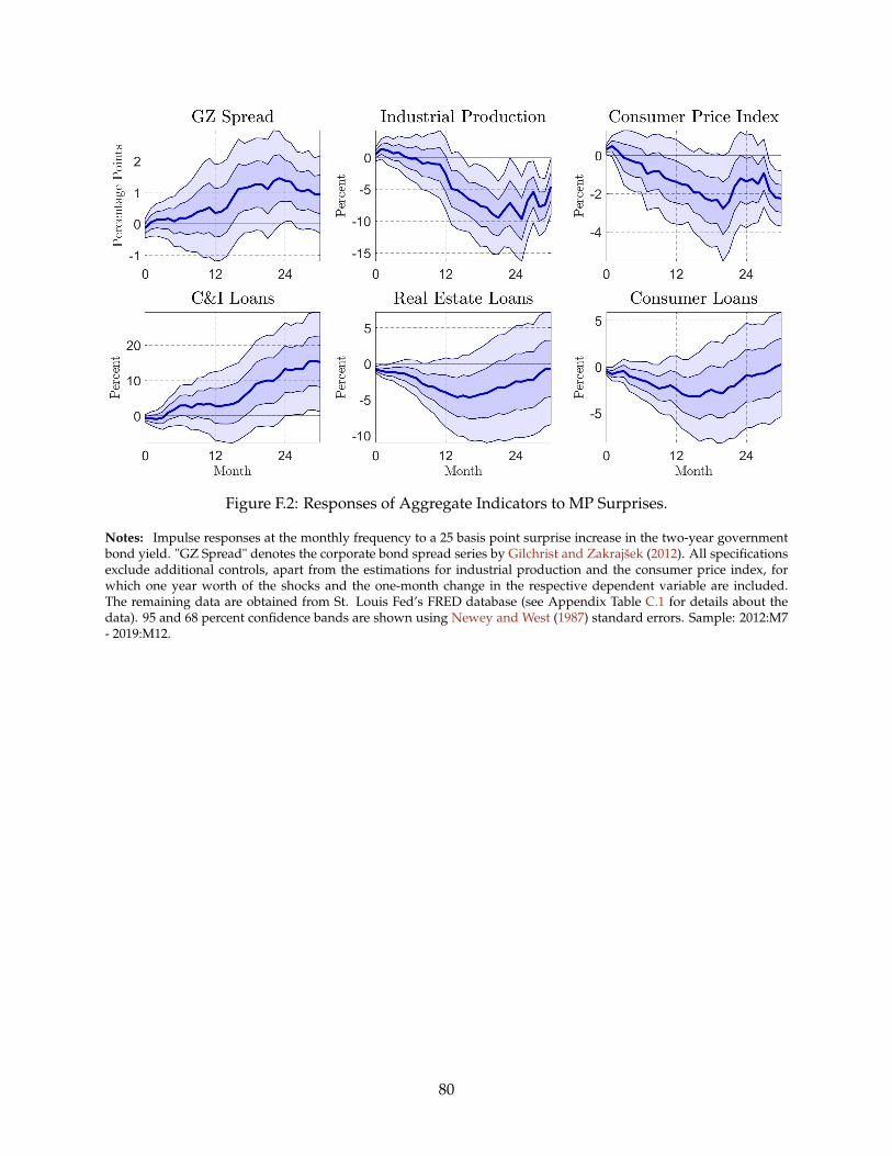
Figure F.2: Responses of Aggregate Indicators to MP Surprises.

Notes: Impulse responses at the monthly frequency to a 25 basis point surprise increase in the two-year governmentbond yield. "GZ Spread" denotes the corporate bond spread series by Gilchrist and Zakrajšek (2012). All specificationsexclude additional controls, apart from the estimations for industrial production and the consumer price index, forwhich one year worth of the shocks and the one-month change in the respective dependent variable are included.The remaining data are obtained from St. Louis Fed’s FRED database (see Appendix Table C.1 for details about thedata). 95 and 68 percent confidence bands are shown using Newey and West (1987) standard errors. Sample: 2012:M7- 2019:M12.

80

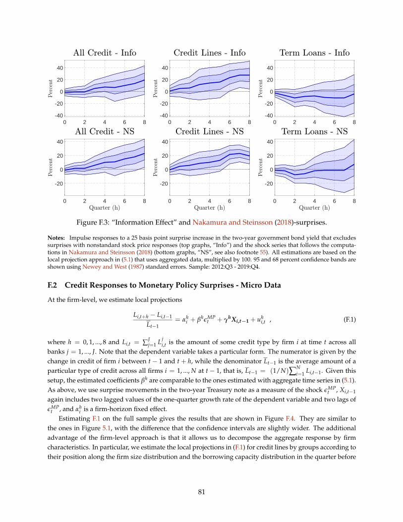
0 2 4 6 8-40

-20

0

20

40

0 2 4 6 8-40

-20

0

20

40

0 2 4 6 8-40

-20

0

20

40

0 2 4 6 8

-20

0

20

40

0 2 4 6 8

-20

0

20

40

0 2 4 6 8

-20

0

20

40

Figure F.3: “Information Effect” and Nakamura and Steinsson (2018)-surprises.

Notes: Impulse responses to a 25 basis point surprise increase in the two-year government bond yield that excludessurprises with nonstandard stock price responses (top graphs, “Info”) and the shock series that follows the computa-tions in Nakamura and Steinsson (2018) (bottom graphs, “NS”, see also footnote 55). All estimations are based on thelocal projection approach in (5.1) that uses aggregated data, multiplied by 100. 95 and 68 percent confidence bands areshown using Newey and West (1987) standard errors. Sample: 2012:Q3 - 2019:Q4.

F.2 Credit Responses to Monetary Policy Surprises - Micro Data

At the firm-level, we estimate local projections

Li,t+h − Li,t−1

Lt−1= αh

i + βhεMPt + γhXi,t−1 + uh

i,t , (F.1)

where h = 0, 1, ..., 8 and Li,t = ∑Jj=1 Lj

i,t is the amount of some credit type by firm i at time t across allbanks j = 1, ..., J. Note that the dependent variable takes a particular form. The numerator is given by thechange in credit of firm i between t− 1 and t + h, while the denominator Lt−1 is the average amount of aparticular type of credit across all firms i = 1, ..., N at t− 1, that is, Lt−1 = (1/N)∑N

i=1 Li,t−1. Given thissetup, the estimated coefficients βh are comparable to the ones estimated with aggregate time series in (5.1).As above, we use surprise movements in the two-year Treasury note as a measure of the shock εMP

t , Xi,t−1

again includes two lagged values of the one-quarter growth rate of the dependent variable and two lags ofεMP

t , and αhi is a firm-horizon fixed effect.

Estimating F.1 on the full sample gives the results that are shown in Figure F.4. They are similar tothe ones in Figure 5.1, with the difference that the confidence intervals are slightly wider. The additionaladvantage of the firm-level approach is that it allows us to decompose the aggregate response by firmcharacteristics. In particular, we estimate the local projections in (F.1) for credit lines by groups according totheir position along the firm size distribution and the borrowing capacity distribution in the quarter before

81

the shock occurs.58 We separate firms into three groups of similar size and rescale their response by thenumber of firms in each group relative to the total number of firms for each respective estimation. Theresults are shown in Figures F.5 and F.6. The total response of credit lines is almost entirely explained byfirms that are large and have substantial ex-ante borrowing capacity.59

0 2 4 6 8

-20

0

20

0 2 4 6 8

-20

0

20

0 2 4 6 8

-20

0

20

Figure F.4: Firm-Level Credit Responses to a Monetary Policy Surprise.

Notes: Impulse responses of firms’ total used credit, credit lines, and term loans to a 25 basis point surprise increase ofthe two-year government bond yield based on the local projection approach in (F.1), multiplied by 100. The estimationsare based on a balanced panel and include 235,225 observations for credit lines, 286,934 for term loans, and 498,384 forall credit for each impulse response horizon. 95 and 68 percent confidence bands are shown using Driscoll and Kraay(1998) standard errors. Sample: 2012:Q3 - 2019:Q4.

58Firm size is measured by total assets, and borrowing capacity is the amount of unused credit, combining unusedcredit lines and term loans. In Figure F.6, we consider two versions for firms’ borrowing capacity, an unadjusted one,where unused credit is given by the difference between committed credit and used credit, and one that additionallyadjusts unused credit for generic covenant rules (see Appendix C.2 for details).

59In separate regressions, we confirm that the responses of large firms and the ones with large unused borrowingcapacity are also statistically different from the responses of either of the two other groups around the seven-quarter-ahead impulse response horizon at the one standard deviation confidence intervals. Differences in the magnitude ofthe total responses between Figures 5.1, F.4, F.5, and F.6 may arise because of variations in the sample of firms arisingfrom differences in the data availability that is used in each respective estimation.

82

0 2 4 6 8-50

0

50

0 2 4 6 8-50

0

50

0 2 4 6 8-50

0

50

Figure F.5: Credit Line Responses by Firm Size.

Notes: Impulse responses of firms’ credit lines to a 25 basis points surprise increase of the two-year government bondyield based on the local projection approach in (F.1), multiplied by 100. The estimations are based on a balanced paneland include a total of 88,941 observations for each respective impulse response horizon. Firms are separated into threebins of equal size according to their position along the firm size distribution in the quarter before the shock occurs.95 and 68 percent confidence bands are shown using Driscoll and Kraay (1998) standard errors. Sample: 2012:Q3 -2019:Q4.

0 2 4 6 8

-10

0

10

20

30

0 2 4 6 8

-10

0

10

20

30

0 2 4 6 8

-10

0

10

20

30

0 2 4 6 8

-20

0

20

40

0 2 4 6 8

-20

0

20

40

0 2 4 6 8

-20

0

20

40

Figure F.6: Credit Line Responses by Borrowing Capacity.

Notes: Impulse responses of firms’ credit lines to a 25 basis points surprise increase of the two-year government bondyield based on the local projection approach in (F.1), multiplied by 100. Firms are separated into three bins of similarsize according to their position along the borrowing capacity distribution in the quarter before the shock occurs. Thetop graphs use firms’ total unused borrowing as a measure of borrowing capacity, and the bottom graphs additionallyadjust this measure for generic covenant rules (see Appendix C.2 for details). The estimations are based on a balancedpanel and include a total of 235,225 observations (top figures), and 84,088 observations (bottom figures), respectively,for each impulse response horizon. 95 and 68 percent confidence bands are shown using Driscoll and Kraay (1998)standard errors. Sample: 2012:Q3 - 2019:Q4.

83

F.3 Credit Movements during the COVID-19 Pandemic

To further understand which firms accounted for the drawdowns on existing credit lines and how thosefirm characteristics changed relative to other periods, we estimate a set of regressions,

Yi,t = αt + τk + β1Xi,t−1 + β2Xi,t−1 · It + ui,t , (F.2)

where Xi,t−1 is a vector of firm characteristics, It is an indicator variable that is equal to one in 2020:Q1and zero otherwise, and Yi,t is one of three possible dependent variables. In the first specification, it isgiven by the log-odds ratio of a (0-1)-indicator, determining whether a firm draws on an existing creditline from one quarter to the next (column (i) of Table F.1). Along the intensive margin, column (ii) con-siders the change in the use of an existing credit line, where the functional form is again given by 2 ·(Li,t − Li,t−1) / (Li,t + Li,t−1) to account for possible zero observations and diminish the influence of ex-treme observations. We also specify a change of an existing credit line measure that is scaled by laggedaverage credit line use across all firms as a way of detecting which type of firms account for the aggregatechange in utilization, (Li,t − Li,t−1) /Lt−1 (column (iii) in Table F.1).60 Besides the time- and industry-fixedeffects αt and τk, the same set of explanatory variables is used as in Section 4.1, apart from using net incomeinstead of EBITDA as a measure of profitability.61 The interaction terms are intended to uncover whetherthe usual financing patterns may have changed in 2020:Q1.

Similar to the findings in Section 4.2, the negative coefficient on “Net Income” suggests that firms drawon their credit lines when they experience low profits in normal times. However, at the onset of the pan-demic, this relationship flips, such that previously profitable firms access their credit lines. A similar patternoccurs for the variables “Size” and “Public,” as well as for “Borrowing Capacity” at the extensive margin.Thus, in 2020:Q1, the type of firms that access their existing credit lines are different than in normal times:large, profitable, publicly traded firms with preestablished borrowing capacity draw on their availablefunding. In addition, highly leveraged firms and firms rated below investment grade are more likely to usetheir credit lines.

60Li,t and Li,t−1 in columns (ii) and (iii) of Table F.1 denote credit lines that were established in t− 1 or prior to that

date. Lt−1 is the average credit line use across all firms in t− 1, that is, Lt−1 = (1/N)∑Ni=1 Li,t−1.

61To eliminate outliers and data entry errors, observations within the 1 percent tails of the distributions for netincome, tangible assets (both relative to noncash assets), and leverage are excluded.

84

Table F.1: COVID-19 − Changes in Existing Credit Lines.

(i) (ii) (iii)Draw Existing Line ∆ Existing Line ∆ Existing Line

(0,1)-Dummy 2 · (Li,t − Li,t−1)/(Li,t + Li,t−1) (Li,t − Li,t−1)/Lt−1

Coeff. Std.Err. Coeff. Std.Err. Coeff. Std.Err.

Borrowing Capacity -0.34*** 0.02 -0.77*** 0.01 -1.49*** 0.05· × It -0.53*** 0.06 -0.59*** 0.03 -0.51*** 0.19Net Income -0.11*** 0.05 -0.04*** 0.02 -0.31*** 0.04· × It -0.44*** 0.12 -0.22*** 0.06 -1.65*** 0.26Tangible Assets -0.73*** 0.03 -0.08*** 0.01 -0.05*** 0.03· × It -0.59*** 0.08 -0.00*** 0.04 -0.19*** 0.29Size -0.02*** 0.00 -0.00*** 0.00 -0.09*** 0.01· × It -0.05*** 0.01 -0.04*** 0.01 -0.82*** 0.09Leverage -0.77*** 0.04 -0.07*** 0.01 -0.17*** 0.04· × It -0.01*** 0.09 -0.06*** 0.05 -1.90*** 0.42Investment Grade -0.16*** 0.01 -0.02*** 0.01 -0.13*** 0.03· × It -0.04*** 0.05 -0.04*** 0.02 -0.09*** 0.23Public -0.17*** 0.03 -0.12*** 0.01 -0.34*** 0.04· × It -0.39*** 0.07 -0.15*** 0.04 -5.59*** 0.61Firm Age -0.02*** 0.01 -0.00*** 0.00 -0.03*** 0.01· × It -0.02*** 0.02 -0.02*** 0.01 -0.09*** 0.14

Sum of Coefficients 2020:Q1Borrowing Capacity -0.19*** 0.06 -1.37*** 0.03 -2.00*** 0.18Net Income -0.33*** 0.11 -0.17*** 0.06 -1.35*** 0.25Tangible Assets -1.32*** 0.08 -0.09*** 0.04 -0.13*** 0.28Size -0.03*** 0.01 -0.03*** 0.01 -0.73*** 0.09Leverage -0.79*** 0.09 -0.13*** 0.05 -2.06*** 0.42Investment Grade -0.20*** 0.04 -0.06*** 0.02 -0.04*** 0.22Public -0.22*** 0.07 -0.03*** 0.04 -5.25*** 0.61

Firm Age -0.00*** 0.02 -0.03*** 0.01 -0.06*** 0.14R-squared 0.04 0.08 0.03Observations 260,766 183,457 260,766

Number of Firms 41,563 32,900 41,563

Notes: Estimation results for firm credit regressions (F.2) using changes in existing credit lines from one quarter tothe next. Dependent variables are a {0,1}-variable measuring whether a firm drew on an existing credit line in column(i), the change in used credit of an existing credit line, relative to a firm’s own stock over two quarters in column (ii)or the average existing credit line stock in the previous quarter in column (iii). All explanatory variables are given bythe most recent observations over the previous four quarters. Borrowing capacity is the share of unused borrowing tototal commitments. Net income and tangible assets are scaled by noncash assets (total assets minus cash and marketablesecurities). Size is defined as the natural log of noncash assets. Leverage is the ratio of total liabilities to total assets. Firmage is the natural log of the number of periods between the observation date and firm incorporation date, annualized.The incidence of a firm drawing on an existing credit line is estimated as a logit regression, reporting a Pseudo R2. Allother specifications are estimated using OLS. All estimations include time and industry fixed effects. Standard errorsin parentheses are clustered by firm. Sample: 2012:Q3 - 2020:Q1. ∗∗∗p < 0.01, ∗∗p < 0.05, ∗p < 0.1.

85

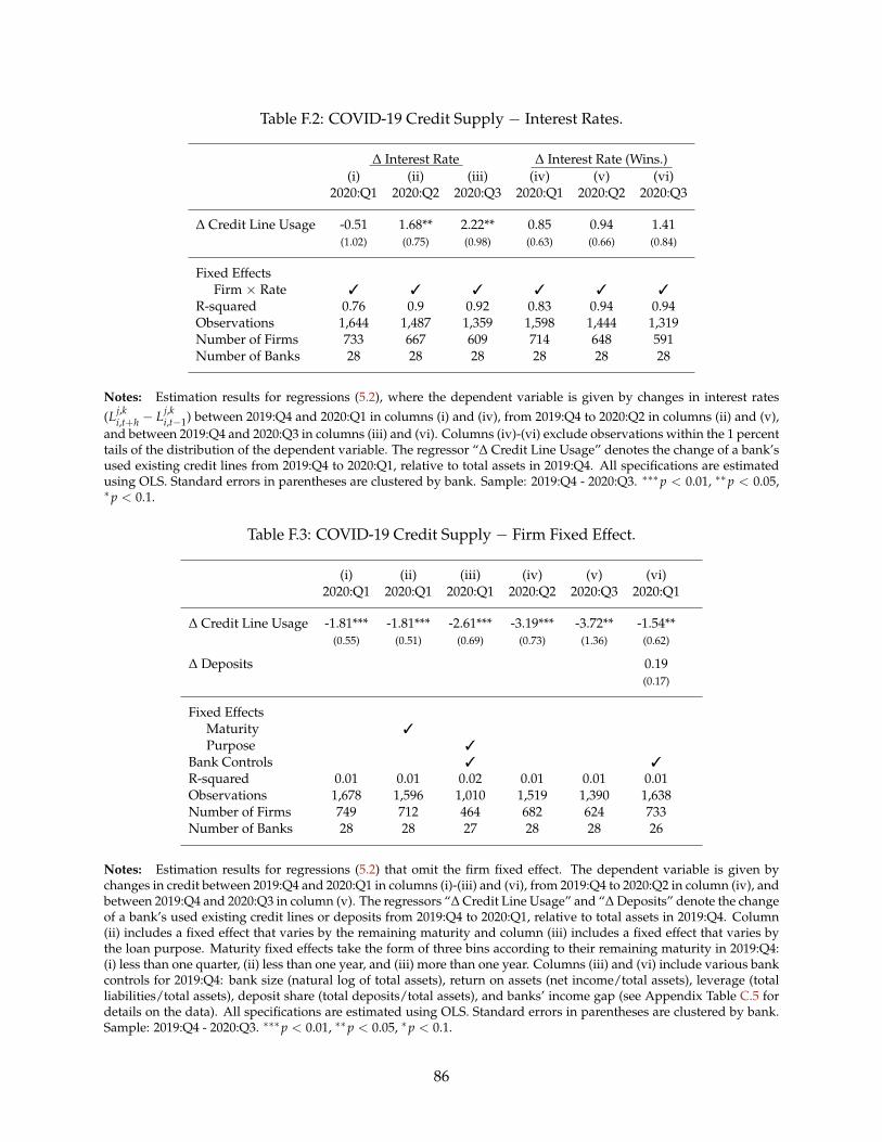
Table F.2: COVID-19 Credit Supply − Interest Rates.

∆ Interest Rate ∆ Interest Rate (Wins.)(i) (ii) (iii) (iv) (v) (vi)

2020:Q1 2020:Q2 2020:Q3 2020:Q1 2020:Q2 2020:Q3

∆ Credit Line Usage -0.51 1.68** 2.22** 0.85 0.94 1.41(1.02) (0.75) (0.98) (0.63) (0.66) (0.84)

Fixed Effects∗∗ Firm × Rate 3 3 3 3 3 3

R-squared 0.76 0.9 0.92 0.83 0.94 0.94Observations 1,644 1,487 1,359 1,598 1,444 1,319Number of Firms 733 667 609 714 648 591Number of Banks 28 28 28 28 28 28

Notes: Estimation results for regressions (5.2), where the dependent variable is given by changes in interest rates(Lj,k

i,t+h − Lj,ki,t−1) between 2019:Q4 and 2020:Q1 in columns (i) and (iv), from 2019:Q4 to 2020:Q2 in columns (ii) and (v),

and between 2019:Q4 and 2020:Q3 in columns (iii) and (vi). Columns (iv)-(vi) exclude observations within the 1 percenttails of the distribution of the dependent variable. The regressor “∆ Credit Line Usage” denotes the change of a bank’sused existing credit lines from 2019:Q4 to 2020:Q1, relative to total assets in 2019:Q4. All specifications are estimatedusing OLS. Standard errors in parentheses are clustered by bank. Sample: 2019:Q4 - 2020:Q3. ∗∗∗p < 0.01, ∗∗p < 0.05,∗p < 0.1.

Table F.3: COVID-19 Credit Supply − Firm Fixed Effect.

(i) (ii) (iii) (iv) (v) (vi)2020:Q1 2020:Q1 2020:Q1 2020:Q2 2020:Q3 2020:Q1

∆ Credit Line Usage -1.81*** -1.81*** -2.61*** -3.19*** -3.72** -1.54**(0.55) (0.51) (0.69) (0.73) (1.36) (0.62)

∆ Deposits 0.19(0.17)

Fixed Effects∗∗Maturity 3

∗∗ Purpose 3

Bank Controls 3 3

R-squared 0.01 0.01 0.02 0.01 0.01 0.01Observations 1,678 1,596 1,010 1,519 1,390 1,638Number of Firms 749 712 464 682 624 733Number of Banks 28 28 27 28 28 26

Notes: Estimation results for regressions (5.2) that omit the firm fixed effect. The dependent variable is given bychanges in credit between 2019:Q4 and 2020:Q1 in columns (i)-(iii) and (vi), from 2019:Q4 to 2020:Q2 in column (iv), andbetween 2019:Q4 and 2020:Q3 in column (v). The regressors “∆ Credit Line Usage” and “∆ Deposits” denote the changeof a bank’s used existing credit lines or deposits from 2019:Q4 to 2020:Q1, relative to total assets in 2019:Q4. Column(ii) includes a fixed effect that varies by the remaining maturity and column (iii) includes a fixed effect that varies bythe loan purpose. Maturity fixed effects take the form of three bins according to their remaining maturity in 2019:Q4:(i) less than one quarter, (ii) less than one year, and (iii) more than one year. Columns (iii) and (vi) include various bankcontrols for 2019:Q4: bank size (natural log of total assets), return on assets (net income/total assets), leverage (totalliabilities/total assets), deposit share (total deposits/total assets), and banks’ income gap (see Appendix Table C.5 fordetails on the data). All specifications are estimated using OLS. Standard errors in parentheses are clustered by bank.Sample: 2019:Q4 - 2020:Q3. ∗∗∗p < 0.01, ∗∗p < 0.05, ∗p < 0.1.

86

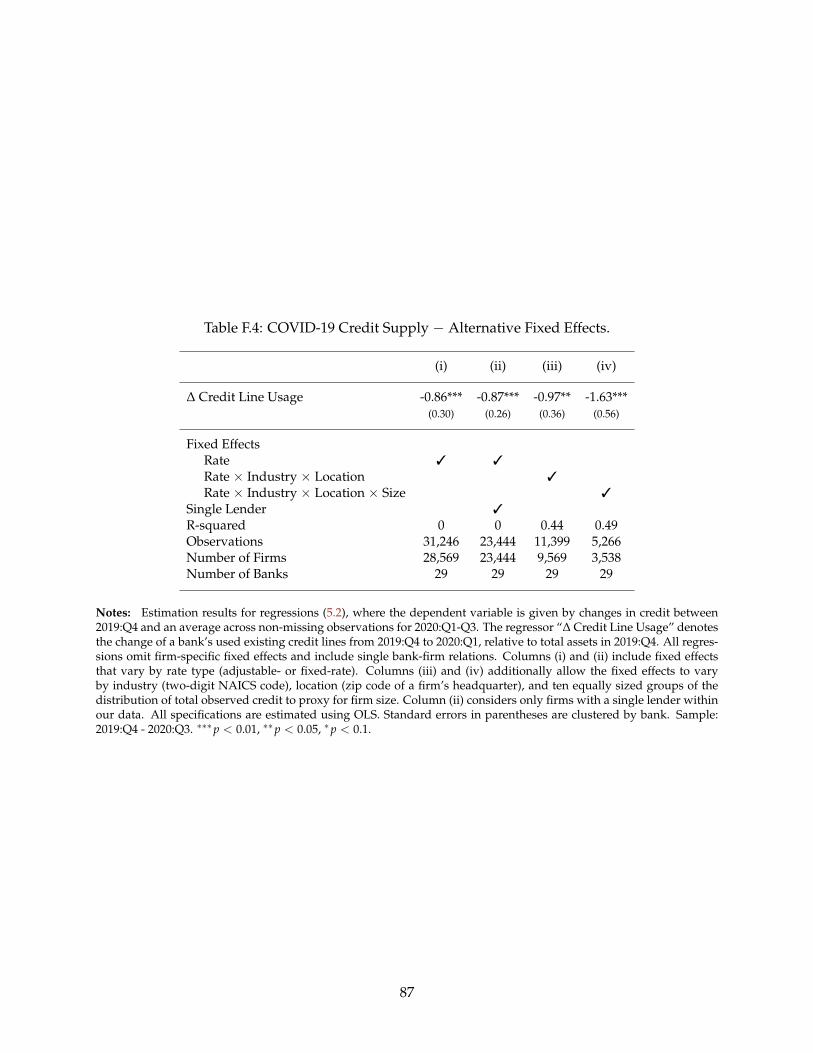
Table F.4: COVID-19 Credit Supply − Alternative Fixed Effects.

(i) (ii) (iii) (iv)

∆ Credit Line Usage -0.86*** -0.87*** -0.97** -1.63***(0.30) (0.26) (0.36) (0.56)

Fixed Effects∗∗ Rate 3 3

∗∗ Rate × Industry × Location 3

∗∗ Rate × Industry × Location × Size 3

Single Lender 3

R-squared 0 0 0.44 0.49Observations 31,246 23,444 11,399 5,266Number of Firms 28,569 23,444 9,569 3,538Number of Banks 29 29 29 29

Notes: Estimation results for regressions (5.2), where the dependent variable is given by changes in credit between2019:Q4 and an average across non-missing observations for 2020:Q1-Q3. The regressor “∆ Credit Line Usage” denotesthe change of a bank’s used existing credit lines from 2019:Q4 to 2020:Q1, relative to total assets in 2019:Q4. All regres-sions omit firm-specific fixed effects and include single bank-firm relations. Columns (i) and (ii) include fixed effectsthat vary by rate type (adjustable- or fixed-rate). Columns (iii) and (iv) additionally allow the fixed effects to varyby industry (two-digit NAICS code), location (zip code of a firm’s headquarter), and ten equally sized groups of thedistribution of total observed credit to proxy for firm size. Column (ii) considers only firms with a single lender withinour data. All specifications are estimated using OLS. Standard errors in parentheses are clustered by bank. Sample:2019:Q4 - 2020:Q3. ∗∗∗p < 0.01, ∗∗p < 0.05, ∗p < 0.1.

87

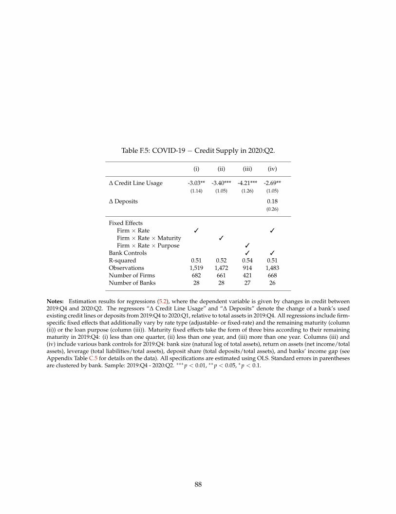
Table F.5: COVID-19 − Credit Supply in 2020:Q2.

(i) (ii) (iii) (iv)

∆ Credit Line Usage -3.03** -3.40*** -4.21*** -2.69**(1.14) (1.05) (1.26) (1.05)

∆ Deposits 0.18(0.26)

Fixed Effects∗∗ Firm × Rate 3 3

∗∗ Firm × Rate ×Maturity 3

∗∗ Firm × Rate × Purpose 3

Bank Controls 3 3

R-squared 0.51 0.52 0.54 0.51Observations 1,519 1,472 914 1,483Number of Firms 682 661 421 668Number of Banks 28 28 27 26

Notes: Estimation results for regressions (5.2), where the dependent variable is given by changes in credit between2019:Q4 and 2020:Q2. The regressors “∆ Credit Line Usage” and “∆ Deposits” denote the change of a bank’s usedexisting credit lines or deposits from 2019:Q4 to 2020:Q1, relative to total assets in 2019:Q4. All regressions include firm-specific fixed effects that additionally vary by rate type (adjustable- or fixed-rate) and the remaining maturity (column(ii)) or the loan purpose (column (iii)). Maturity fixed effects take the form of three bins according to their remainingmaturity in 2019:Q4: (i) less than one quarter, (ii) less than one year, and (iii) more than one year. Columns (iii) and(iv) include various bank controls for 2019:Q4: bank size (natural log of total assets), return on assets (net income/totalassets), leverage (total liabilities/total assets), deposit share (total deposits/total assets), and banks’ income gap (seeAppendix Table C.5 for details on the data). All specifications are estimated using OLS. Standard errors in parenthesesare clustered by bank. Sample: 2019:Q4 - 2020:Q2. ∗∗∗p < 0.01, ∗∗p < 0.05, ∗p < 0.1.

88

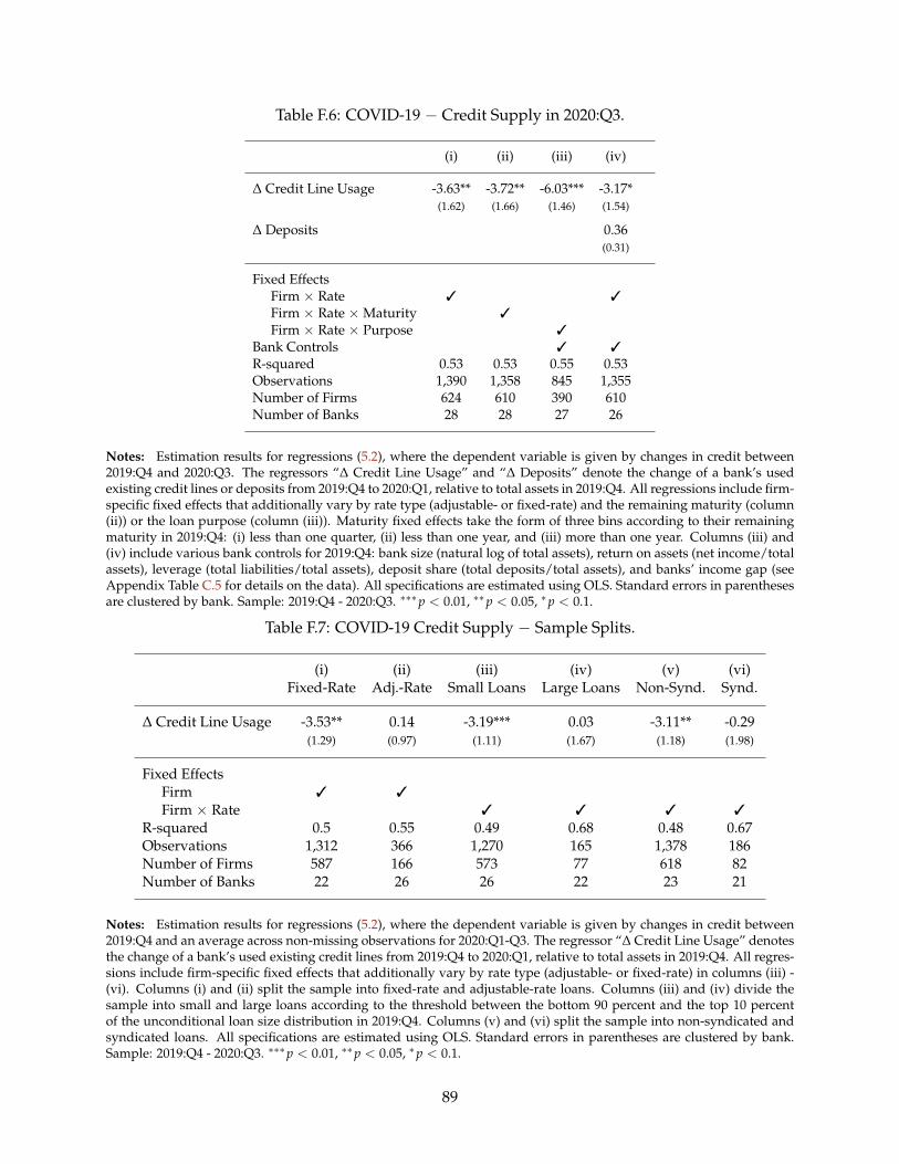
Table F.6: COVID-19 − Credit Supply in 2020:Q3.

(i) (ii) (iii) (iv)

∆ Credit Line Usage -3.63** -3.72** -6.03*** -3.17*(1.62) (1.66) (1.46) (1.54)

∆ Deposits 0.36(0.31)

Fixed Effects∗∗ Firm × Rate 3 3

∗∗ Firm × Rate ×Maturity 3

∗∗ Firm × Rate × Purpose 3

Bank Controls 3 3

R-squared 0.53 0.53 0.55 0.53Observations 1,390 1,358 845 1,355Number of Firms 624 610 390 610Number of Banks 28 28 27 26

Notes: Estimation results for regressions (5.2), where the dependent variable is given by changes in credit between2019:Q4 and 2020:Q3. The regressors “∆ Credit Line Usage” and “∆ Deposits” denote the change of a bank’s usedexisting credit lines or deposits from 2019:Q4 to 2020:Q1, relative to total assets in 2019:Q4. All regressions include firm-specific fixed effects that additionally vary by rate type (adjustable- or fixed-rate) and the remaining maturity (column(ii)) or the loan purpose (column (iii)). Maturity fixed effects take the form of three bins according to their remainingmaturity in 2019:Q4: (i) less than one quarter, (ii) less than one year, and (iii) more than one year. Columns (iii) and(iv) include various bank controls for 2019:Q4: bank size (natural log of total assets), return on assets (net income/totalassets), leverage (total liabilities/total assets), deposit share (total deposits/total assets), and banks’ income gap (seeAppendix Table C.5 for details on the data). All specifications are estimated using OLS. Standard errors in parenthesesare clustered by bank. Sample: 2019:Q4 - 2020:Q3. ∗∗∗p < 0.01, ∗∗p < 0.05, ∗p < 0.1.

Table F.7: COVID-19 Credit Supply − Sample Splits.

(i) (ii) (iii) (iv) (v) (vi)Fixed-Rate Adj.-Rate Small Loans Large Loans Non-Synd. Synd.

∆ Credit Line Usage -3.53** 0.14 -3.19*** 0.03 -3.11** -0.29(1.29) (0.97) (1.11) (1.67) (1.18) (1.98)

Fixed Effects∗∗ Firm 3 3

∗∗ Firm × Rate 3 3 3 3

R-squared 0.5 0.55 0.49 0.68 0.48 0.67Observations 1,312 366 1,270 165 1,378 186Number of Firms 587 166 573 77 618 82Number of Banks 22 26 26 22 23 21

Notes: Estimation results for regressions (5.2), where the dependent variable is given by changes in credit between2019:Q4 and an average across non-missing observations for 2020:Q1-Q3. The regressor “∆ Credit Line Usage” denotesthe change of a bank’s used existing credit lines from 2019:Q4 to 2020:Q1, relative to total assets in 2019:Q4. All regres-sions include firm-specific fixed effects that additionally vary by rate type (adjustable- or fixed-rate) in columns (iii) -(vi). Columns (i) and (ii) split the sample into fixed-rate and adjustable-rate loans. Columns (iii) and (iv) divide thesample into small and large loans according to the threshold between the bottom 90 percent and the top 10 percentof the unconditional loan size distribution in 2019:Q4. Columns (v) and (vi) split the sample into non-syndicated andsyndicated loans. All specifications are estimated using OLS. Standard errors in parentheses are clustered by bank.Sample: 2019:Q4 - 2020:Q3. ∗∗∗p < 0.01, ∗∗p < 0.05, ∗p < 0.1.

89

Table F.8: COVID-19 Credit Supply − Bank Capital.

(i) (ii) (iii)2020:Q1 2020:Q2 2020:Q3

∆ Credit Line Usage -5.16*** -8.72*** -13.95***(1.15) (1.94) (3.08)

∆ Credit Line Usage × Cap-Buffer 1.29** 2.30** 3.88***(0.52) (0.88) (1.34)

Cap-Buffer -0.01** -0.02** -0.04***(0.01) (0.01) (0.02)

Fixed Effects: Firm × Rate 3 3 3

Bank Controls 3 3 3

R-squared 0.51 0.51 0.53Observations 1,650 1,493 1,365Number of Firms 738 672 614Number of Banks 27 27 27

Notes: Estimation results for regressions (5.2), where the dependent variable is given by changes in credit between2019:Q4 and 2020:Q1 (column (i)), 2020:Q2 (column (ii)), or 2020:Q3 (column (iii)). The regressor “∆ Credit Line Usage”denotes the change of a bank’s used existing credit lines from 2019:Q4 to 2020:Q1, relative to total assets in 2019:Q4.“Cap-Buffer" denotes banks’ voluntary capital buffers in 2019:Q4, which are defined as the difference between commonTier 1 capital ratios and (4.5 + SCB + GSIB) where SCB is the stress capital buffer and GSIB is the additional buffer forglobal systemically important banks. “∆ Credit Line Usage × Cap-Buffer" denotes the interaction between the twovariables. All specifications include various bank controls for 2019:Q4: bank size (natural log of total assets), return onassets (net income/total assets), leverage (total liabilities/total assets), deposit share (total deposits/total assets), andbanks’ income gap (see Appendix Table C.5 for details on the data). Standard errors in parentheses are clustered bybank. Sample: 2019:Q4 - 2020:Q3. ∗∗∗p < 0.01, ∗∗p < 0.05, ∗p < 0.1.

90

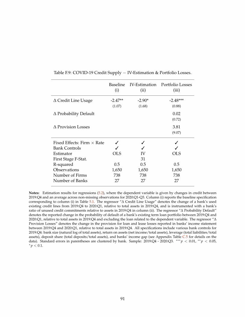
Table F.9: COVID-19 Credit Supply − IV-Estimation & Portfolio Losses.

Baseline IV-Estimation Portfolio Losses(i) (ii) (iii)

∆ Credit Line Usage -2.47** -2.90* -2.48***(1.07) (1.68) (0.88)

∆ Probability Default 0.02(0.72)

∆ Provision Losses 3.81(9.07)

Fixed Effects: Firm × Rate 3 3 3

Bank Controls 3 3 3

Estimator OLS IV OLSFirst Stage F-Stat. 31R-squared 0.5 0.5 0.5Observations 1,650 1,650 1,650Number of Firms 738 738 738Number of Banks 27 27 27

Notes: Estimation results for regressions (5.2), where the dependent variable is given by changes in credit between2019:Q4 and an average across non-missing observations for 2020:Q1-Q3. Column (i) reports the baseline specificationcorresponding to column (i) in Table 5.1. The regressor “∆ Credit Line Usage” denotes the change of a bank’s usedexisting credit lines from 2019:Q4 to 2020:Q1, relative to total assets in 2019:Q4, and is instrumented with a bank’sratio of unused credit commitments relative to assets in 2019:Q4 in column (ii). The regressor “∆ Probability Default”denotes the reported change in the probability of default of a bank’s existing term loan portfolio between 2019:Q4 and2020:Q1, relative to total assets in 2019:Q4 and excluding the loan related to the dependent variable. The regressor “∆Provision Losses” denotes the change in the provision for loan and lease losses reported in banks’ income statementbetween 2019:Q4 and 2020:Q1, relative to total assets in 2019:Q4. All specifications include various bank controls for2019:Q4: bank size (natural log of total assets), return on assets (net income/total assets), leverage (total liabilities/totalassets), deposit share (total deposits/total assets), and banks’ income gap (see Appendix Table C.5 for details on thedata). Standard errors in parentheses are clustered by bank. Sample: 2019:Q4 - 2020:Q3. ∗∗∗p < 0.01, ∗∗p < 0.05,∗p < 0.1.

91

Table F.10: COVID-19 − Total Debt & Cash.

∆ Total Debt ∆ Cash

All Small/Large All Small Large(i) (ii) (iii) (iv) (v)

∆ Credit Line Usage -2.63***(0.69)

∆ Credit Line Usage × Small -2.61***(0.68)

∆ Credit Line Usage × Large 0.97(5.72)

∆ Total Debt 0.07*** 0.07*** -0.87(0.01) (0.01) (0.78)

Industry Fixed Effects 3 3 3 3 3

Firm Controls 3 3 3 3 3

Estimator OLS OLS IV IV IVFirst Stage F-Stat. 233 167 10.9R-squared 0.08 0.08 0.02 0.18 0.02Observations 3,164 3,164 3,163 1,572 1,590Number of Firms 3,164 3,164 3,163 1,572 1,590Number of Banks 28 28 28 23 28

Notes: Columns (i) and (ii) report estimation results for regressions (5.3). “∆ Credit Line Usage” denotesthe estimation results for β. Column (ii) additionally distinguishes the effect by firm size, where a large firmis defined as one with total assets within the top 20 percent of the firm size distribution in 2019 and the indi-cator variable is included in the set of firm controls. Columns (iii)-(v) report estimation results for the instru-mental variable regressions (Cashi,t+1 − Cashi,t−3)/Assetsi,t−3 = αm + β · 2

(Di,t+1 − Di,t−1

)/(

Di,t+1 + Di,t−1)+

γ Xi,t−1 + ui,t+1, where Cashi,t denotes cash holdings at time t and the timing is chosen to match the one in Ta-

ble 5.2. The variables ∑Jj=1 ω

ji,t−1(∆Credit Line Usagej

t)/Assetsjt−1 and ∑J

j=1 ωji,t−1 are used as instruments for

2(

Di,t+1 − Di,t−1)

/(

Di,t+1 + Di,t−1). “∆ Total Debt” denotes the estimation results for β. Xi,t−1 includes ∑J

j=1 ωji,t−1

in columns (i) and (ii) and various firm indicators in 2019:Q2: net income, cash, tangible assets, total liabilities (all rela-tive to total assets), firm size (natural log of total assets), and a binary variable that indicates whether a firm is publiclytraded. Columns (iv) and (v) restrict the sample by firm size following the definition in column (ii). All specificationsinclude industry fixed effects (two-digit NAICS code). Standard errors in parentheses are clustered by the bank withthe largest term loan to firm i. Sample: 2019:Q2 - 2020:Q2. ∗∗∗p < 0.01, ∗∗p < 0.05, ∗p < 0.1.

92

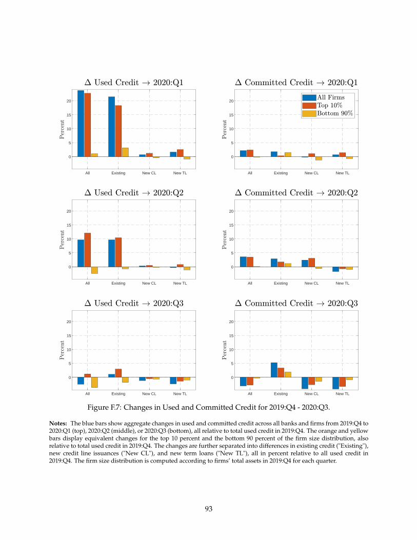
All Existing New CL New TL

0

5

10

15

20

All Existing New CL New TL

0

5

10

15

20

All Existing New CL New TL

0

5

10

15

20

All Existing New CL New TL

0

5

10

15

20

All Existing New CL New TL

0

5

10

15

20

All Existing New CL New TL

0

5

10

15

20

Figure F.7: Changes in Used and Committed Credit for 2019:Q4 - 2020:Q3.

Notes: The blue bars show aggregate changes in used and committed credit across all banks and firms from 2019:Q4 to2020:Q1 (top), 2020:Q2 (middle), or 2020:Q3 (bottom), all relative to total used credit in 2019:Q4. The orange and yellowbars display equivalent changes for the top 10 percent and the bottom 90 percent of the firm size distribution, alsorelative to total used credit in 2019:Q4. The changes are further separated into differences in existing credit ("Existing"),new credit line issuances ("New CL"), and new term loans ("New TL"), all in percent relative to all used credit in2019:Q4. The firm size distribution is computed according to firms’ total assets in 2019:Q4 for each quarter.

93