The Cross-Sectional Relation between Distress Risk Premiums

and the Explanatory Power of Structural Models

December 31, 2014§

Abstract

We investigate the effect of CDS-implied distress risk premiums on the

explanatory power of structural models on CDS spreads. Interestingly, we find

that the cross-sectional variation in the power can be attributed to a few of

factors, especially to the ratio of distress risk premium to CDS spread. Our

analysis reveals the negative relation between distress risk premium

proportion in CDS spreads and the explanatory power of structural models.

Structural variables inspired by theory are more likely to fail to account for

CDS spreads of firms with higher distress risk premiums in a given level of

spreads. Based on this evidence, we argue that the distress risk premium

embedded in CDS spreads is a culprit that hampers empirical studies using the

structural approach. We also find evidence that the distress risk premiums are

not related to firm-specific default rates. Rather, the main driving forces of the

distress risk premiums are the market-wide factors. Several robustness checks

also support our results.

JEL Classification: G12; G13; E32

Keywords: distress risk premium, credit default swap, structural models, reduce-form approach

§ This is a very preliminary version. Please do not cite this article without any permission of the authors.

1

1. Introduction

The option pricing model by Black and Scholes (1973) and Merton (1974) has been one of

the most successful works in finance literature over the past few decades. Nevertheless,

application of the model, typically referred to as a structural approach, to the pricing of

corporate debt is not as satisfactory. While the Merton model and its many variants are

theoretically elegant, a substantial amount of papers report that the structural models do quite

a poor job in accounting for empirical prices of corporate bonds. For example, Jones et al.

(1984), Eom et al. (2004), and Huang and Huang (2012) calibrate many Merton-kind

structural models to historical bond price data and find that any structural models, even

though incorporating realistic and complicated features, hardly match model prices to those

observed in the market. Most structural models they investigate underestimate market prices.

As such, the failure of the structural approach has been rather surprising to academics.

After such negative findings of the calibration studies, another strand of literature has

instead used a linear regression model, and has tried to confirm whether structural variables

inspired by theory are important determinants to explain the variation in corporate spreads or

credit default swap (CDS) spreads. For instance, Collin-Dufresne et al. (2001) and Ericsson

et al. (2009) not only show that structural variables such as leverage ratio, asset volatility,

and riskless short rate are statistically significant for explaining corporate yield spreads or

CDS spreads, they also confirm that the signs of the estimates are consistent with theory.

However, the findings using a lineal regression model are still questionable to academics.

These findings are that the change in corporate spreads is significantly unexplained by the

change in the structural factors. The previous studies show that in the change regressions, the

explanatory power of the model is, at most, about 20% in terms of average R2 and the

residuals of the model for each firm have (economically unknown but statistically

pronounced) systematic co-movements; we also confirm these phenomena with our sample.

In this study, we place particular focus on the cross-sectional variation in the explanatory

powers rather than on the low average. Although the body of literature has made an effort to

increase such a strikingly low explanatory power of structural variables by adding possibly

2

omitted variables, none of them have paid attention to the cross-sectional variation in the

explanatory power. Compared to previous studies, it is true that the average explanatory

power of structural variables is similarly low (about 26.8% on average) in our sample.

However, we find that the power is very different from firm to firm and, more interestingly,

the variation seems systematic. For instance, while the explanatory power is 0.8% for

Franklin Resources, Inc., it is as much as 78.7% for Lehman Brothers Holdings Inc. This

finding motivates us to examine whether the significant variation is systematic or trivial. In

other words, we ask whether it is attributable to some firm-specific characteristics or to

something else or is attributable to nothing. Thus, the purpose of our study is explaining why

the variation exists and what it may be attributed to.

Intuition suggests that a distress risk premium implicit in CDS spreads can be a culprit to

weaken an explanatory power of structural variables on CDS spreads since the individual

distress risk premium would not be explained by the structural variables but instead market-

wide risk premiums would drive it. Before identifying the reasons, we may illustrate the

distress risk premium (DRP hereafter) with intuitive words. Consider two CDS contracts for

firms A and B which have the same expected default probabilities, whatever they are

measured by (e.g., structural variables such as the leverage ratio and asset volatility, or rating,

etc.). The only difference between the two firms is the extent to which their conditional

default risk varies over time in an unexpected way. For example, the asset value of firm A

could be highly sensitive to unpredictable changes in market covariates, and subsequently,

the firm is more likely to suffer from severe and unexpected ups-and-downs of its conditional

default rate than the other firm is likely to. All else being equal, CDS sellers should command

a higher CDS spread for firm A than firm B because when they offer an insurance for the

event of firm A’s default, they would have more exposure to unexpected changes in

conditional default risk. In other words, CDS sellers would require a compensation for

bearing distress risk, and hence, they command DRP in addition to a spread for the

conditionally expected default risk, implying that the same expected default rate does not

necessarily lead to the same level of CDS spreads. Therefore, we can guess that CDS spreads

include DRPs.

3

From this intuition, it is easy to summarize the hypotheses we test and research design

by three steps. First, we expect that a significant amount of DRP is involved in a given CDS

spread and its proportion differs from various firms. One of the challenges to examining this

may lie on estimating the DRP contained in CDS spreads. To address the econometrics issue,

we borrow the novel idea proposed by Pan and Singleton (2008) to estimate DRPs from CDS

data with a single factor affine term structure model. Pan and Singleton (2008) explicitly

specify the market price of risk associated with unexpected changes in instantaneous default

probability and estimate CDS term structures under both risk-neutral and physical measures,

which allows one to identify the related risk premium by taking a difference between the

risk-neutral and physical expectations on future default risk.

Second, we conjecture that individual DRPs are driven by market-wide risk premiums

rather than by firm-specific variables which determine the firm-specific conditional default

rate. It is reasonable to say that, if the DRP estimated by the PS model is a good measure for

our purpose so that it can isolate the risk premium part from the other part caused by expected

default rates in a CDS spread, the individual DRP should only respond to the fluctuation of

aggregate risk premiums observed in the financial markets, and it would not be related to

individual expected default rate measures. Conversely, testing this hypothesis can be viewed

as testing whether the PS model-implied DRP is a good estimate for the purpose of our study.

Given the estimated DRPs, testing this hypothesis is quite straightforward. We regress either

DRP or DRP proportion on several market risk premiums. Guided by literature, we employ

aggregate risk premiums stemming from three important financial markets. First, from the

bond market we obtain the risk-free rate measured by the ten-year Treasury bond yield

(Collin-Dufresne et al. 2001; Ericsson et al. 2009), term premium measured by difference

between 20 year and 1 year U.S. Treasury yields and default premium measured by the

difference between yields on Baa and Aaa corporate bonds (Chen et al., 1986). The Treasury

yield and term premium also can be interpreted as the level and slope factors of interest rate

risk from the term structure model’s perspective (Duffie and Kan, 1996). Second, from the

stock market we obtain three equity risk premiums, the so called, MKT, SMB, and HML

(Fama and French, 1993) and market liquidity risk premium (Pástor and Stambaugh, 2003).

4

Third, from the option market we consider the variance risk premium measured by the VIX

minus realized volatility of the S&P 500 in the spirit of Bollerslev et al. (2009), Carr and Wu

(2009), Todorov (2009), and Wang et al. (2013). In addition to the regression, we also test

firm-specific variables such as leverage ratio and asset volatility measured by historical

volatility of individual stock returns or option-implied volatility to confirm that DRPs are not

related to firm-specific determinants of conditional default rates.

Finally and most important, we hypothesize that a DRP involved in a CDS spread

hampers the structural variables from explaining the CDS spreads. In other words, we expect

that, for firms with a higher DRP in a given CDS spread, the explanatory power of structural

variables on their CDS spread would be weaker. This hypothesis naturally arises from the

results of the aforementioned two tests. As expected above, if the movement of individual

DRPs is not relevant to firm-specific conditional default rates, it would be more difficult to

explain the time variation of CDS spreads only with firm-specific variables measuring the

conditionally expected default rates especially for firms with higher DRP proportion in their

CDS spreads. Thus, we expect to find out a decreasing pattern in explanatory power with

DRP proportion. To test the hypothesis, we follow the conventional procedure that has been

commonly employed in the literature on cross-section of expected stock returns; that is,

sorting, examining any pattern, testing the difference between extreme groups, controlling

for other characteristics, and regressing the patterned value on potential attributes. Being

familiar with literature on the returns on stock, one may easily understand our research

method if he or she substitutes the object of the study from expected stock returns to

explanatory power measures of Merton model regressions. In doing so, we measure the firm-

by-firm explanatory power by both adjusted R2 and root-mean-squared-errors (RMSE) which

are obtained from the changes regressions of the CDS spread on the Merton variables, as a

bench-mark linear model like previous studies. The specific tests are as follows. First, we

sort all firms into five groups based on their DRP proportions, examine, if any exist,

decreasing patterns in the cross-section of explanatory power, and test statistical significance

in the difference between the average explanatory power of two extreme groups. Next, to

control for other firm-specific characteristics, we repeat the test 3-by-3 independent double-

5

sorts based on DRP proportions and one of the firm-specific control variables including the

leverage ratio, historical volatility, implied volatility, rating, stock liquidity and CDS liquidity.

Finally, to begin formal testing, we estimate cross-sectional regressions. The dependent

variable of the regression is adjusted R2 values from the Merton model, and the independent

variables include the time-series average of the tested attributes, namely, DRP proportion,

leverage ratio, historical volatility, implied volatility, rating, stock liquidity, and CDS

liquidity.

The empirical findings are quite consistent with our conjectures. First, a sizable portion

of CDS spreads is due to DRP. On median, while the level of an individual CDS spread is

104 bps, the level of DRP is 34 bps, amounting to 33% of a given CDS spread. The DRP and

its proportion are statistically different from zero with significant cross-sectional variations

of 119 bps and 68%, respectively. In addition, the individual DRP and its proportion fluctuate

over time as well.

Next, we find that both the DRP and its proportion of individual firms systematically

respond to the movements of market-wide factors, but there is no evidence that they are

relevant to firm-specific expected default rates. Specifically, a variety of market risk

premiums are statistically and economically significant for explaining the changes in DRP

and DRP proportion both in univariate and multivariate regressions at a conventional

significance level. In the test of the significance of firm-specific default rates, leverage ratio,

historical volatility, and implied volatility are all significant, seeming to be contrary to our

prediction. However, after controlling for the market-wide risk factors, the significance of

firm-specific default risk factors is all subsumed, suggesting that seemingly significant

effects of the firm-specific default risks are due to somewhat correlated information with

market-wide risk premiums. For example, the effect of leverage disappears when we control

for Fama-French three factors. It can be justified by the notion that the variation in leverage

of a firm is mostly driven by the variation in its equity price, and the equity price is strongly

affected by Fama-French pricing factors. Similarly, it is not surprising that the market-wide

volatility premium subsumes the effects of individual historical and implied volatilities.

6

Furthermore, we find evidence that explanatory power of the bench-mark regression

decreases with the amount of DRP in a given CDS spread. In the univariate sort analysis, we

find a monotonically decreasing pattern of average adjusted R2 for the bench-mark model,

showing that 29%, 27%, 23%, 21% and 19% from the lowest to the highest DRP proportion

group. The difference between the explanatory power of two extreme groups is statistically

significant with a t-statistic of 5.04. In the bivariate sort analysis, we also find that the

monotonically decreasing patterns and statistically significant difference in all groups

controlled for firm-specific characteristics including the leverage ratio, historical and implied

volatility, rating, stock liquidity, and CDS liquidity. The only exception is for the lowest and

the next leverage groups. The patterns are slightly inverted V-shape, but the difference

between the extreme groups along the dimension of DRP proportion is still marginally

significant.

Our findings are also confirmed by a variety of robustness checks. We conduct robustness

tests in two fronts. First, we replicate the results with an alternative measure for DRPs

proposed by Friewald et al. (2014). Second, we repeat the analysis with the subsample

excluding the recent financial crisis period. Due to the limit of space, not all results are

reported, but we show that the main findings remain intact. That is, we confirm the

monotonically decreasing pattern with the alternative DRP measure and in the subsample

period.

Our study relates and contributes to the literature in three aspects. First, the results of our

study have implications that time-varying market-wide risk premiums should be considered

in modelling credit risk. A number of papers have shown that market-wide variables have an

impact on CDS or/and bond spreads although it cannot be reconciled within the Merton

framework. For example, Hackbarth et al. (2006), Chen (2010), and Tang and Yan (2010)

argue that macroeconomic risk is an important factor in structural models. Collin-Dufresne

et al. (2001) and Ericsson et al. (2009) test market variables such as the VIX, the S&P 500,

the yield curve slope, etc. in their regression analysis. Galil et al. (2014) also show that Fama

and French's (1993) three factors and Chen et al.'s (1986) five factors have a statistical

significance for CDS spread changes. Wang et al. (2013) take the market-wide variance risk

7

premium into account in order to explain CDS spreads. From our perspective, the efforts of

these studies can be viewed as proxying for distress risk premiums which cannot be captured

by firm-related default factors. We add another empirical evidence that market-wide factors

beyond the structural variables play an important role in explaining CDS spreads in a

different way.

Second, we contribute to the literature by comprehensive speculation on a variety of

attributes which are related to the systematic difference in explanatory power or pricing errors

of a structural model. So far as we know, little empirical study has been done on explaining

the systematic variation in pricing errors or explanatory power. Only two exceptions are

Jones et al. (1984) and Eom et al. (2004). In their calibration experiments, they find that

pricing errors are systemically related to several firm-characteristics including leverage ratio,

asset volatility, bond maturity, bond rating, etc. Among the tested characteristics, they argue

that leverage ratio has the most significant effect on pricing errors. Although we address the

same question in a different framework (that is, with a linear regression rather than non-linear

calibration), our findings are consistent with theirs. Moreover, we find another important

dimension, or a DRP to which the previous studies have not paid attention. We provide strong

evidence that the amount of DRPs in CDS spreads are a very significant dimension related

to the explanatory power, even after controlling for the firm-characteristics that have been

shown as important factors related to pricing errors in the previous studies.

Finally, to the best of our knowledge, this study is the first in the literature on CDS/bond

spread models, in that we investigate cross-sectional variation in explanatory power of linear

regressions, while most previous studies have tried to increase low average explanatory

power (e.g., Collin-Dufresne et al. 2001; Alexander and Kaeck 2008; Das et al. 2009;

Ericsson et al. 2009; Zhang et al. 2009; Cao et al. 2010; Tang and Yan 2010; Wang et al. 2013;

Galil et al. 2014; among others). A better understanding of cross-variation in explanatory

power of structural models will help better price contingent claims on credit risk and devise

a better model for them.

The rest of this article proceeds as follows. Section 2 implements a preliminary analysis

to show the cross-sectional variation in the explanatory power. Our main findings are shown

8

in section 3. In section 4, we examine robustness for the results in several ways. We replicate

the main findings with an alternative measure of DRPs and the subsample excluding the

recent financial crisis period. Section 5 discusses the reason why structural models do a

particularly poor job in explaining CDS spread changes with an illustration of a simulation

study. Finally, we conclude in section 6. Appendix in the end describes the econometrical

details about estimating DRP measures and calculating explanatory variables.

2. Cross-sectional variation in explanatory power of structural variables

Before empirically testing the aforementioned hypotheses, we confirm the empirical

findings of previous studies with our sample. By doing so, not only do we prove that our

sample is qualitatively the same with that of literature while this study covers rather a

different period and firms; we also introduce new empirical findings that have motivated this

study, i.e., the cross-sectional variation in the explanatory power of the structural models.

To compare the results of previous studies such as Collin-Dufresne et al. (2001) and

Ericsson et al. (2009), the bench-mark structural model we test throughout this paper is the

Merton model. The Merton model suggests that the likelihood of default of a firm is

determined by three variables or structural variables5: i) leverage ratio, ii) asset volatility, iii)

risk-free rate. We will test the explanatory power of the Merton model with a linear regression.

Hence, the specification of level regressions is given as:

𝐶𝐷𝑆𝑖,𝑡 = 𝛽0 + 𝛽1𝐿𝐸𝑉𝑖,𝑡 + 𝛽2𝐻𝑉𝑖,𝑡 + 𝛽3𝐼𝑉𝑖,𝑡 + 𝛽4𝑅𝐹𝑡 + 휀𝑖,𝑡 , (1)

and similarly, the specification of change regressions is as below:

Δ𝐶𝐷𝑆𝑖,𝑡 = 𝛽0 + 𝛽1Δ𝐿𝐸𝑉𝑖,𝑡 + 𝛽2Δ𝐻𝑉𝑖,𝑡 + 𝛽3Δ𝐼𝑉𝑖,𝑡 + 𝛽4Δ𝑅𝐹𝑡 + 휀𝑖,𝑡, (2)

where LEV, HV, IV, and RF denote the leverage ratio, historical volatility, implied volatility,

and risk-free rate, respectively, and ΔXt = Xt − Xt−1 represents their differences. Refer to

5 Throughout the paper, we use the terminology of Merton variables and structural variables interchangeably. In any case, they

indicate the leverage ratio, asset volatility, and risk-free rate.

9

the data section and appendix for the details on the source of the data and method to calculate

the variables.

[Insert Table 1 about here]

Table 1 shows the similar result with that in previous studies. That is, the structural

variables are statistically and economically significant for explaining both the level and

change of CDS spreads. In addition, it is also consistent with the literature that the average

R2 notably drops in the change regressions, as shown in Panel B. Specifically, while the R2

of the level regression of M3 is about 72% on average, it drops to 27% for the corresponding

change regression. The significant drop of explanatory power is similarly observed in all

specifications from M1 to M3 even though the coefficients of the structural variables retain

the similar values in the level and change regressions. This implies that the ability of

structural model to explain the change in CDS spreads is much poorer than the ability to

explain the level for some reasons. Despite all previous papers’ efforts to increase the average

explanatory power of the structural models, the poor performance of the change regression

has remained and it has been a puzzle to academics.

This paper shifts attention from increasing the low average explanatory power to

explaining a reason for the poor performance of the Merton model. What has captured our

interest is cross-sectional variation of the R2s rather than the average value of them. As shown

in the bottoms of each panel of Table 1, there exists significant variation in the R2s firm-by-

firm. In the M3 change regression, for example, the ability of the Merton model is merely 5%

for the five percentile firm. In contrast, it is as much as 54%, as measured by R2, for the 95

percentile firm. That is, even though the Merton model does a poor job on explaining CDS

spread changes on average, the model is quite a good for some firms while it completely fails

for other firms.

Thus, we examine whether there exists a reason for such variation. Should we be able to

attribute the variation to any firm characteristics, it may signpost for structural approach to

resolving the puzzle. Furthermore, as explained before, we expect that one of the reasons

10

would be a DRP which is contained in a CDS spread but not related to firm-specific structural

variables.

3. Empirical analysis

3.1 Data

Monthly observations of CDS spreads come from Markit. Compared with the stock prices

and firms’ accounting data, CDS data are available only for a relatively short period, hence

our sample period based on the availability of CDS data range from January 2001 to

November 2012. We limit our attention to the U.S. corporate CDS spreads with modified

restructuring (MR) for dollar-denominated senior unsecured debt. Throughout the paper, we

analyze CDS spreads maturing in five-years. However, term structure data are also necessary

for estimating DRPs by using the Pan and Singleton’s (2008) model. For the estimation

purpose, we require that firms have CDS spread observations for one-, five-, and ten-year

maturity contracts. In addition, based on the Markit’s sector classification, we exclude firms

in the utility sector which are typically protected by the government and hence the default

risk of them may be rather different from that of the other private firms.

To calculate Merton variables such as leverage ratio and asset volatility, we should obtain

daily equity prices and quarterly accounting data for the sample firms. To this end, we first

link the Center for Research on Security Prices (CRSP) database to the COMPUSTAT

database. Next, by Entitycusip from Markit's Reference Entity Database (RED), we match

the CRSP/COMPUSTAT merged database to the CDS sample obtained above. After merging

all databases, only firms which have monthly observations more than 20 are selected in order

to avoid spurious results from regressions. Finally, we are left with 388 firms and 40,397

firm-month observations.

3.1.1 Identifying DRPs implicit in CDS spreads

As previously explained, insight suggests that CDS spreads generally include premiums

for distress risk, as defined by DRPs, as well as for expected default risk. Our econometrical

challenge is to disentangle a DRP from a CDS spread. Our approach to modeling and

11

estimating DRP implicit in CDS spreads closely follows the work of Pan and Singleton (2008)

who employ the idea that a risk premium for future change in default risk is priced in the

difference between expectations under risk-neutral and physical measures.6

Our model is constructed as follows. First, we assume that conditional instantaneous

default risk is driven by a single factor. In particular, we assume that (risk-neutral) intensity

𝜆𝑄 follows a log-normal process with Brownian motion 𝑊𝑃 under the physical (or P)

measure:

𝑑 ln 𝜆𝑄 = 𝜅𝑃(𝜃𝑃 − ln 𝜆𝑄)𝑑𝑡 + 𝜎𝑑𝑊𝑃 . (3)

Next, we specify the market price of risk by 𝛬𝑡 = 𝛿0 + 𝛿1 ln 𝜆𝑡𝑄

so that the stochastic

movement of intensity follows 𝑑𝑊𝑄 = 𝑑𝑊𝑃 + 𝛬𝑑𝑡 under the risk-neutral (or Q) measure

and the log-normal property of the intensity process remains even after the change of measure.

The market price of risk allows us to measure a risk premium associated with the future

change in default risk. With this setting, we can obtain the model price of a CDS and estimate

the model parameters related to intensity process as well as the market-price-of-risk process

(Appendix A1 provides the detail).

The unpredictable future change in default risk, which is instantaneously captured by

𝜎𝑑𝑊𝑃, is priced in a CDS spread in the way of 𝜅𝑄 = 𝜅𝑃 + 𝛿1𝜎 and 𝜅𝑄𝜃𝑄 = 𝜅𝑃𝜃𝑃 − 𝛿0𝜎.

Thus, the risk premium associated with volatility risk of the conditional default risk (note

that this model is doubly stochastic) is implicit in the difference between Q-expected default

probability and P-expected default probability.

To extract the implicit risk premium (or DRP), we compute a ‘pseudo-CDS spread’ with

the physical default probability (P-measure) as in Pan and Singleton (2008). Specifically, the

pseudo-CDS spread, denoted by 𝐶𝐷𝑆𝑃 , is computed by using the estimated parameters

under the P-measure (i.e., using 𝜅𝑃 and 𝜃𝑃 instead of 𝜅𝑄 and 𝜃𝑄 ), while the model

spread of a CDS is computed by using the estimated parameters under the Q-measure. We

6 This idea is further used by, for example, Longstaff et al. (2011), Díaz et al. (2013), Zinna (2013), and Friewald et al. (2014) to

study CDS-implied risk premiums.

12

note that, in general, the rule of risk-neutral pricing of contingent claims suggests that a model

CDS spread should be calculated under the Q-measure (Harrison and Kreps, 1979). Thus, the

additional spread due to the risk premium, denoted by DRP, can be obtained from the

difference between the model spread and the psuedo-spread, i.e., the DRP for firm i at time t

is defined by

𝐷𝑅𝑃𝑖,𝑡 ≡ 𝐶𝐷𝑆𝑖,𝑡 − 𝐶𝐷𝑆𝑖,𝑡𝑃 . (4)

Also, we define DRP proportion as the ratio of DRP to CDS spread

𝑝𝑖,𝑡𝐷𝑅𝑃 ≡

𝐷𝑅𝑃𝑖,𝑡

𝐶𝐷𝑆𝑖,𝑡, (5)

which measures how much amount is due to distress risk in a given CDS spread.

We illustrate the implications of DRPs with a numerical example. To demonstrate the

effect of the premium for distress risk on a CDS spread, we change the volatility parameter

σ from zero to one, keeping P-expected default risk within five years constant, and we

calculate corresponding model spreads of a CDS with a maturity of five years.

[Insert Figure 1 about here]

Figure 1 displays the model spread of a five year CDS for different σ values while the

expected default probability under the P-measure is kept as 0.05, 0.10, or 0.15. Consistent

with the intuition, it shows that higher distress risk causes higher CDS spreads even though

the P-expected default probability (and in turn 𝐶𝐷𝑆𝑃) is constant. For example, controlling

for the P-expected default probability as 0.10, we see that 𝐶𝐷𝑆 is the same with 𝐶𝐷𝑆𝑃 as

124 bps for no distress risk, i.e., σ = 0, while 𝐶𝐷𝑆, showing 350 bps, is approximately

twice as higher as 𝐶𝐷𝑆𝑃 for the highest distress risk, i.e., σ = 1. In the case of the highest

distress risk, 𝐷𝑅𝑃 = 226bps and 𝑝𝐷𝑅𝑃 = 64%. This numerical experiment suggests that

the presence of DRPs increases the level of CDS spreads, explicitly showing our intuition on

DRPs. Even if conditionally expected default risks are the same for two firms, investors

would command a higher CDS spread for a firm with highly unpredictable change in the

13

future default risk because they want a compensation for the higher distress risk as well as

the default risk. In the next section, we will show the empirical results regarding DRPs with

real data.

3.1.2 Descriptive statistics

Descriptive statistics for the estimated DRP and the explanatory variables are reported in

Table 2. Except for market variables, the other statistics are obtained from individual

averages for each firm. With regard to CDS spreads, the overall mean of the averages from

each firm is about 162 bps and the standard deviation is about 174. This large standard

deviation indicates that our sample include firms with various credit levels. Not only the

spreads but the estimated DRP also shows large variation among the firms. The averages

range from the five percentile of -130 bps to the 95 percentile of 181 bps. Negative risk

premiums on CDS spreads are also found in Longstaff et al. (2011). In their research there is

a country that has a negative median of the risk premium. Since credit qualities of the

companies in our sample are distributed widely and each series behavior of spreads is various,

several firms have extremely negative or positive risk premiums. The median of the averages

of DRP is about 34 bps and this value is a little bit larger than that of Díaz et al. (2013) where

they estimate risk premiums from European corporate CDS data. Like the DRP, averages of

DRP proportion also exhibit large variation across the firms. Since DRP proportion is the

relative size of the risk premium, from the median for the averages of DRP proportion we

see that DRP occupies a large portion of the total CDS spread. The 37 percent of the median

percentage is about a third of the spread.

[Insert Table 2 about here]

Next, we focus on confirming the time series variation of DRP and DRP proportion. In

Figure 2 and Figure 3, we plot cross-sectional averages of the DRP and the DRP proportion

over time. To show the relation between DRP and the market states preliminarily, market or

macroeconomic variable levels are plotted together. The empirical features are summarized

in three points. First, the aggregate DRP and DRP proportion exhibit positive values most of

14

the time, and it reveals that investors require premiums on expected future changes of credit

worthiness on average. Second, the time series behavior of the aggregate DRP and DRP

proportion varies considerably. The means of DRP and DRP proportion sore especially

during the Global Financial Crisis (GFC), and we see that not only the default risk but the

distress risk is high during that time. After the GFC, the level of DRP falls, whereas DRP

proportion maintains high levels continuously. It shows that investors tend to require a large

portion of the risk premium after they experience a large shock in markets. Lastly, DRP and

DRP proportion exhibit the strong relation with the market variables. In particular, DRP and

DRP proportion are closely related to the default premium and the term premium,

respectively.

[Insert Figure 2 about here]

[Insert Figure 3 about here]

3.2 DRPs are driven by market-wide risk premiums

This section explores what determine the time variations of the individual corporate

distress risk premiums. Given that our DRP truly estimates a compensation for unpredictable

changes in conditional default risk, the DRP is likely to respond to the movements of market-

wide risk premiums because a firm value (and subsequently conditional default risk) co-

varies with the state of the economy. As shown before, indeed, the aggregate DRP and DRP

proportion vary markedly over time, and particularly, they co-moves with a couple of market-

wide factors, suggesting that the individual CDS-implied distress risk premium could be

potentially related to several market risk premiums. Thus, we examine whether the individual

DRP and DRP proportion are driven by a variety of market-wide risk premiums or firm-

specific structural variables, or both. We expect that aggregate risk premiums would drive

the individual DRPs because the DRP is a risk premium for bearing the unexpected change

in default risk. In addition, the firm-specific variables which measure the conditionally

expected default rates would have nothing to do with the individual DRPs.

3.2.1 The effect of aggregate risk premiums

15

We start by running firm-by-firm regressions of either a DRP or a DRP proportion as a

dependent variable yi,t on a set of aggregate risk premiums as explanatory variables

including the risk-free rate (RF), variance risk premium (VRP), three equity risk premiums

(MKT, SMB, and HML), liquidity risk premium (PSLIQ), term premium (UTS), and

corporate default premium (UPR). The time-series regression for firm i is nested within the

following specification:

𝛥𝑦𝑖,𝑡 = 𝛽0 + 𝛽1𝛥𝑅𝐹𝑡 + 𝛽2𝛥𝑉𝑅𝑃𝑡 + 𝛽3𝑀𝐾𝑇𝑡 + 𝛽4𝑆𝑀𝐵𝑡 + 𝛽5𝐻𝑀𝐿𝑡 + 𝛽6𝑃𝑆𝐿𝐼𝑄𝑡

+ 𝛽7𝛥𝑈𝑇𝑆𝑡 + 𝛽8𝛥𝑈𝑃𝑅𝑡 + 휀𝑖,𝑡 . (6)

Note that MKT, SMB, HML and PSLIQ are not differenced as they are the returns on factor

mimicking portfolios. Except those variables, all variables are differenced. Table 3 presents

the result; the dependent variable is DRP in Panel A while it is DRP proportion in Panel B.

Following Collin-Dufresne et al. (2001) and Ericsson et al. (2009), parameter estimates and

adjusted R2 are averaged across firm-by-firm regressions and associated t-statistics are

calculated for the average estimates.

[Insert Table 3 about here]

As expected, both of individual DRPs and DRP proportions are driven by the aggregate

risk premiums we test. Specifically, several results are noteworthy. First, the coefficients are

statistically and economically significant in the simple and multiple regressions. Except for

some cases showing marginal significance, the aggregate risk premiums from the three

important markets are all significant at the most conservative level or 1%, for explaining the

movements of DRPs as well as DRPs per unit spread (or DRP proportion), which suggests

that DRPs and DRP proportions are strongly related to the aggregate risk premiums. This

also provides evidence that the credit derivative market is closely linked to the other financial

markets. In particular, it is interesting that the market liquidity risk premium (PSLIQ) has

something to do with the individual DRPs measured in the CDS market.

In addition, adding all the market-wide risk premiums in a multiple regression shows that

all the variables hold their significance for explaining the DRPs per unit spread (see M6 in

16

Panel B of Table 3). The evidence is slightly weak for the regression of individual DRPs, but

the MKT factor and equity market liquidity risk premium are statistically and economically

significant.

Finally, we note that the signs of the coefficients of premiums are the same for both DRPs

regressions and DRP proportions regressions. For example, the risk-free rate, MKT and SMB

factors, and equity market liquidity risk premium are negatively related to the individual

DRPs and DRP proportions, whereas the variance risk premium, HML factor, term premium,

and default premium are positively related to the individual DRPs and DRP proportions (see

M1-M5 in Table 3).

In sum, whether we measure CDS-implied risk premiums by an amount or its proportion,

we verify that individual CDS-implied risk premiums are closely related to the aggregate risk

premiums of other financial markets.

3.2.2 The effect of firm-specific default risk factors

Next, we proceed to examine whether the individual DRPs are affected by firm-specific

determinants of default rates. As before, the dependent variable yi,t is either the DRP or the

DRP proportion for firm i at month t, and the firm-by-firm time-series regressions are nested

in the specification as below:

𝛥𝑦𝑖,𝑡 = 𝛽0 + 𝛽1ΔLEV𝑖,𝑡 + 𝛽2ΔHV𝑖,𝑡 + 𝛽3ΔIV𝑖,𝑡 + 𝛾′𝑋𝑡 + 휀𝑖,𝑡. (7)

where LEV, HV, and IV denote leverage ratio, historical volatility, and implied volatility,

respectively, and the vector X includes all the market-wide risk premiums used in (6). Note

that we here control for the effect of market-wide risk factors Xt.

[Insert Table 4 about here]

When the DRPs or DRP proportions are regressed only on firm-specific structural

variables (or not controlled for market-wide risk factors), we are faced with a somewhat

conflicting result against our prediction (refer to M1 in Table 4). That is, the firm-specific

variables seem to be statistically significant. However, after controlling for the effect of

17

aggregate risk premiums, the significance of them disappears whereas the significance of the

market-wide factors remains (refer to M7 in Table 4). The reason for this could be that the

seemingly significant effects of the firm-specific variables are attributable to the correlated

information with the market-wide factors, which is justified in the result of M2 to M6 in

Table 4. For example, the effect of leverage disappears when we control for Fama-French

three factors, which can be justified by the notion that the variation in leverage of a firm is

mostly driven by the variation in its equity price, and the equity price is strongly affected by

Fama-French pricing factors (see M4). Similarly, it is not surprising that the market-wide

volatility premium subsumes the effects of individual historical and implied volatilities (see

M3). Therefore, the movements of DRPs and DRP proportions are mostly captured by those

of market-wide factors rather than firm-specific variables. Compared to the result of

regression (6) in Table 3, it is particularly interesting that the estimated coefficients and their

significance remain unchanged when we add firm-specific variables in Table 4. That is, the

risk-free rate, MKT and SMB factors, and equity market liquidity risk premium are

negatively related to the individual DRPs and DRP proportions, whereas the variance risk

premium, HML factor, term premium, and default premium are positively related to the

individual DRPs and DRP proportions, as before.

As shown so far, we conclude that the DRPs and DRPs per unit spread are determined by

the aggregate risk premiums. More importantly, we verify that DRPs are not related to firm-

specific determinants of conditionally expected default rates. Conversely, we can conclude

that the model-implied DRP is a good proxy of the DRP we define for our purpose.

3.3 Effect of DRP on the explanatory power of structural models

In this section, we test the hypothesis that a higher DRP leads to weaker explanatory

power of structural models. Regarding

3.3.1 Test model: base regressions

The structural models that we test are linear models and the specification is as follows.

First, for each firm i, we regress the level of CDS spread on a set of structural variables

inspired by the Merton model as below:

18

𝐶𝐷𝑆𝑖,𝑡 = 𝛽0 + 𝛽1𝐿𝐸𝑉𝑖,𝑡 + 𝛽2𝐻𝑉𝑖,𝑡 + 𝛽3𝐼𝑉𝑖,𝑡 + 𝛽5𝑅𝐹𝑡 + 휀𝑖,𝑡, (8)

where the explanatory variables denote leverage, historical volatility, option-implied

volatility, and interest rate, respectively. Second, to investigate the explanatory power of

structural models on change in CDS spreads, we run changes regressions in a similar manner:

Δ𝐶𝐷𝑆𝑖,𝑡 = 𝛽0 + 𝛽1Δ𝐿𝐸𝑉𝑖,𝑡 + 𝛽2Δ𝐻𝑉𝑖,𝑡 + 𝛽3Δ𝐼𝑉𝑖,𝑡 + 𝛽5Δ𝑅𝐹𝑡 + 휀𝑖,𝑡 , (9)

Note that all regressions are time-series regressions and conducted firm-by-firm. As such,

we run both level regressions (8) and change regressions (9) and examine the explanatory

power of the models in several ways as will be shown in subsequent sections.

3.3.2 Cross-sectional variation: R2-approach

Now, we will examine whether the unconditional mean of DRP proportion has any effect

on the explanatory power of structural models in terms of adjusted R2 in level and change

regressions.7 In other words, we test whether cross-sectional differences in adjusted R2, if

any, are attributable to cross-sectional variation of the unconditional mean of DRP proportion.

To this end, we first sort all firms by their average DRP proportions, p̅iDRP, which is

calculated by

�̅�𝑖𝐷𝑅𝑃 =

1

𝑇∑

𝐷𝑅𝑃𝑖,𝑡

𝐶𝐷𝑆𝑖,𝑡

𝑇

𝑡=1

, for 𝑖 = 1, … , 𝑁. (10)

Next, we assign each firm to five groups – that is, from the lowest average DRP proportion

group denoted by G1 to the highest one denoted by G5. For each firm, we obtain adjusted-

R2 from regressions (8) and (9). After that, we compare the average of adjusted-R2 for each

group. The result is plotted in Figure 4 to see a tendency easily and the regression details are

reported in Table 5.

7 To be more conservative, we use adjusted R2 rather than ordinary R2. All results remain intact even if we measure the explanatory

power in terms of ordinary R2.

19

[Insert Figure 4 about here]

The left and right panels of Figure 4 show the pattern of average adjusted-R2 of level and

change regressions, respectively. At a glance, we can see a tendency of adjusted-R2 to

decrease with �̅�𝑖𝐷𝑅𝑃 for all structural models we test. For example, when we add all

structural variables inspired by the Merton model in level regression (refer to M5 in the left

panel of Figure 4), the average adjusted-R2 is 74.8% for the lowest group G1 while it is 59.7%

for the highest group G5. Similarly, in the change regression, we can see that the explanatory

power decreases from 28.9% to 18.5% as a group has more DRP. This tendency is consistent

for all models whether the regressions are implemented in a form of level or change as shown.

Our finding indicates that structural models are more likely to have weak explanatory power

on firms with higher average DRP proportion; or, on average, the more DRP in CDS spreads,

the more likely to fail for structural variables to account for CDS spreads in both level and

change regressions.

To formally test the argument above, we implement t-test on the explanatory power

difference between G1 and G5. In level regressions, the t-statistics of the explanatory power

for G1 minus G5 are 5.98, 5.16, 5.42, 5.34, and 5.04 for M1 to M5, respectively.8 In change

regressions, those are 2.58, 3.30, 4.34, 4.57, and 3.94 for M1 to M5, respectively. As a result,

we strongly reject the null hypothesis (at the 1% level) that average explanatory power of a

structural model is not different from different groups. We instead find evidence that it is

statistically significant that explanatory power for the lowest DRP proportion group G1 is

stronger than that for the highest group G5. Therefore, we confirm again the same result in

this formal test.

[Insert Table 5 about here]

One may wonder if such differential explanatory power stems from insignificance of

structural variables or inconsistency with theory for some groups, especially for G5. But the

8 The t-tests are carried out under an equal-variance assumption. But, the results are almost the same with those under an unequal-

variance assumption.

20

regression details in Table 5 show that it is not the case. Each panel of Table 5 presents the

regression result for each group from G1 to G5. Following Collin-Dufresne et al. (2001) and

Ericsson et al. (2009), we report average estimates and t-statistics for their cross-sectional

average in Table 5. We note that all structural variables are statistically and economically

significant. Also, the signs of the estimates are consistent with theory for all DRP groups.

Since previous studies have already analyzed the meaning of the estimates and it lies outside

of the core of this paper, we do not mention the regression results further. Instead, we

emphasize that structural models are significant for all groups. Nevertheless, the explanatory

power difference is noticeable. Thus, the decreasing tendency of R2 is due to neither

insignificance nor inconsistence with theory for some groups.

From these results, we argue again that the unconditional mean of DRP proportion, �̅�𝐷𝑅𝑃,

has a significant impact on the explanatory power of structural models in both level and

change regressions.

3.3.3 Time variation in the risk premium: RMSE-approach

Next, we will consider the effect of time variation in DRP proportion. In the previous

section, we analyzed the effect of unconditional mean of DRP proportion, but DRP

proportion significantly varies over time. This implies that, for example, a firm with high

average DRP proportion does not necessarily stay in high group at every point of time. The

constituents may differ time to time. As a result, a firm in G1 at a month could be assigned

to G5 next month. We can indeed see in Figure 3 that DRP proportion changes a great deal

over time.

So, we will here test the time-varying effect of DRP proportion by tracking the pricing

errors of the DRP groups evaluated at each point of time. The specific procedure of the test

is as follows. First, as before, we estimate linear structural models (8) and (9) and get time-

series of residuals for each firm9, denoted by εi,t. Then, at month t, we rank all firms by their

9 To be specific, we use studentized residuals rather than ordinary ones. The studentized residuals are standardized version of residuals.

The reason that we choose them in our analysis is as follows. To compare the size of residuals, we should control for the trivial difference

in residuals due to total variation of a dependent variable. For example, when CDS spreads are high, their residuals (or pricing errors) of

models are proportionally getting high; such an effect will lead us to wrong conclusion. This consideration is similar with the fact that R-squared is calculated from not only variation in regressors but also total variation in a dependent variable.

21

month-t DRP proportion, 𝑝𝑖,𝑡𝐷𝑅𝑃, and place them in five bins. We calculate root-mean-squared

errors for group R at month t by

𝑅𝑀𝑆𝐸𝑡𝑅 = √

1

𝑁∑ 휀𝑖,𝑡

𝑅

𝑖=1

, for R = 1(Low), … ,5(High), (11)

where 휀𝑖,𝑡𝑅 denotes the residual for firm i which is ranked at group R at month t. That is, we

track over time the RMSEs for each group ranked based on each month’s DRP proportion.

Finally, we have five time-series of RMSEs: 𝑅𝑀𝑆𝐸𝑡1 for Low to 𝑅𝑀𝑆𝐸𝑡

5 for High.

Similarly with the R2-analysis, we focus on the difference between group 1 and group 5. If

our conjecture that higher DRP proportion leads to weaker explanatory power of structural

models is true, average pricing error for group 5, 𝑅𝑀𝑆𝐸𝑡5, will be consistently higher over

time than those for group 1, 𝑅𝑀𝑆𝐸𝑡1. To statistically test this hypothesis, we perform a t-test

on the time-series difference between group 1 and group 5. If the mean of the difference of

𝑅𝑀𝑆𝐸𝑡1 − 𝑅𝑀𝑆𝐸𝑡

5 is significantly negative, we can infer that pricing errors for G1 (low DRP)

are small, implying a strong explanatory power. This is not a novel idea. In option literature,

for example, Trolle and Schwartz (2009) employ the idea to test pricing performance for

commodity options. We conduct the t-test for pricing errors of the five structural models that

is analyzed in the previous section.

For all models tested, we find strong evidence that structural models have a stronger

explanatory power for group 1(Low DRP) than group 5(High DRP). Specifically, for M1 to

M5, associated t-statistics are -2.55, -3.01, -3.05, -3.03, and -3.07, respectively in level

regressions and those are -3.18, -3.19, -3.14, -3.19, and -3.10, respectively in change

regressions. All these tests reject the null hypothesis at 1% level that the pricing errors are

not significantly different between the two groups. Thus, the result that, for firms with higher

DRP proportion, structural variables are more likely to lose to some extent their explanatory

power on CDS spread levels and changes consistently at every point of time.

3.3.4 Controlling for firm characteristics

22

One can see that the explanatory power of structural models decrease with leverage ratios

from the result of Collin-Dufresne et al. (2001) even though they do not point it out explicitly.

So, one may doubt that the observed pattern of explanatory power in our study can be

attributable to firm-specific characteristics such as the leverage ratio, historical volatility,

option-implied volatility, equity liquidity, CDS liquidity, and credit rating. To verify that the

decreasing pattern is not due to the other firm characteristics, we control for such effects. Our

empirical methodology to address this issue is easy to summarize. We repeat the R2- and

RMSE-analyses as presented in subsection 3.3.2 and 3.3.3. The only difference is that,

instead of univariate-sorting, we double-sort all firms independently based on their DRP

proportions and either of the firm characteristics such as the leverage ratio, historical

volatility, implied volatility, and equity liquidity so that we can control for the effects. To

guarantee the sufficient number of firms in each sort, we assign firms into 3-by-3 sorts in this

analysis. The specific ways of ranking firms and evaluating the measures of the explanatory

power are the same as previously mentioned. Due to the limit of space, we only run the

change regression of Model 5 in the previous section, i.e.,

Δ𝐶𝐷𝑆𝑖,𝑡 = 𝛽0 + 𝛽1Δ𝐿𝐸𝑉𝑖,𝑡 + 𝛽2Δ𝐻𝑉𝑖,𝑡 + 𝛽3Δ𝐼𝑉𝑖,𝑡 + 𝛽5Δ𝑅𝐹𝑡 + 휀𝑖,𝑡 . (12)

Table 6 exhibits that averages of adjusted-R2 for each portfolio sorted on the DRP

proportion and each firm characteristic. The t-statistics of adjusted adjusted-R2 for Group 1

minus Group 3 are positive and significant in all firm characteristics. Except for the group

with low implied volatility, all the other portfolios show significant t-tests regardless of levels

of firm characteristics. In the case of the portfolio with the highest rating, adjusted-R2

declines from 30% to 18% as the average of DRP proportions rises, which shows the

influence of the distress risk premium on explanatory power of Merton variables is not small.

We can also see that the pattern of decreasing adjusted-R2 as the DRP proportion increases

in many cases.

Next, to consider time-varying DRP proportion, we perform the RMSE-analysis in

controlling for the firm characteristics. Table 7 shows that t-statistics for the difference of the

pricing errors. For each level of firm characteristics, the difference between two groups with

23

the lowest and the highest DRP proportions are tested. All t-statistics are negative and

significant except for the group with the highest illiquidity and the highest rating. It indicates

firms with high DRP proportions tend to have poor explanatory power of Merton variables

on CDS spread changes and this tendency is not attributable to individual firm characteristics.

However, though we do not represent the RMSEs in the table, monotonically increasing

patterns of RMSEs as DRP proportion do not appear firmly. So we guess that the existence

of other possibilities that hamper explaining CDS spreads in Merton’s framework.

3.3.5 Cross-sectional regressions

To provide the last evidence on the negative relation between DRP proportions and

explanatory power of structural models, we perform cross-sectional regressions with a

specification nested in the following:

𝑅𝑖2 = 𝛼 + 𝛽 × �̅�𝑖

𝐷𝑅𝑃 + 𝛾′𝑋𝑖 + 휀𝑖 , (13)

where the dependent variable 𝑅𝑖2 is a firm i's adjusted R2 value obtained from the level

regression in (1) and the change regression in (2)10, �̅�𝑖𝐷𝑅𝑃 denotes the time-series average of

DRP proportion of firm i, and Xi is the vector of control variables including the leverage

ratio (LEV), historical volatility (HV), implied volatility (IV), equity illiquidity (ILLIQ),

CDS liquidity (DEPTH), and ratings. All control variables are averaged over the sample

period and standardized in order to compare their importance in the regressions. The

intercepts are zero by construction in every regressions. Refer to Appendix regarding details

of calculating the average ratings of each firm.

Panel A of Table 8 displays the result of the case where we use the level regression

explanatory power as the dependent variable, showing which characteristics the explanatory

power of a level regression model is attributable to. Most importantly, the average DRP

proportion is economically and statistically significant for explaining the cross-sectional

variation in explanatory power of the level regression model. In particular, the coefficient is

10 Thus, (adjusted) R2 values are obtained from the first-pass regressions, and we run the second-pass regressions in (13) by using

the first-pass R2s as a dependent variable.

24

estimated as negative values (ranging from -0.17 to -0.21) for every regressions we

investigate. That is, no matter which variables we control for, the effect of DRP proportion

on the explanatory power of a structural model is negative (and quite stable), consistent with

our hypothesis. This provides an economic implication that an increase in DRP proportion

by one standard deviation leads to a decrease in R2 by approximately 0.2 standard deviation

in a cross-sectional sense. Moving to Panel B, the similar conclusion can be reached, where

we use the change regression explanatory power as the dependent variable of the second-

pass cross-sectional regression. The coefficient of DRP proportion ranges from -0.16 to -0.27

at the 1% significance for every models, which suggests that a structural model in a change

regression does a better job for firms with higher average DRP proportions in explaining

CDS spread changes.

The results also provide some other interesting insights. Whereas the coefficient of the

DRP proportion remains significant and the sign does not alter very much whether the first-

pass regression is level or change (as shown in Panel A and Panel B, respectively), other firm

characteristics have different effects. For example, historical volatility (HV) and credit

ratings (RATING) significantly account for the variation of level regression R2, but not for

the variation of change regression R2. Rather, the leverage ratio and CDS liquidity are

important characteristics accounting for the variation in change regression explanatory power.

This should not be surprising. The level explanatory power is significantly and positively

related to credit ratings (note that in our study a higher value of ratings corresponds to lower

credit quality). This is consistent with previous studies reporting that a structural model has

more difficulty matching empirical credit spreads of investment grade bonds than those of

non-investment grade bonds (see, e.g., Eom et al., 2004; Huang and Huang, 2012).

When it comes to liquidity, M8 of Panel A reveals that the coefficient of ILLIQ -0.13

with a t-statistic of -2.40 while DEPTH is insignificant. In contrast, M8 of Panel B shows

that the coefficient of DEPTH is 0.40 with a t-statistic of 8.59 while ILLIQ is -0.08 and

marginally significant. This suggest that equity liquidity is a more important characteristic

for explaining CDS spread levels, but CDS liquidity plays a more important role in explaining

changes. In addition, the coefficient’s sign implies that firms with illiquid equity has weak

25

explanatory power in level regressions while firms with an illiquid CDS has weak

explanatory power in change regressions. Particularly, noticeable is the role of CDS liquidity

in explaining explanatory power variation on CDS spread changes. In Panel B we see that

the relative size of the coefficient for DEPTH is largest among the characteristics, and it is

most significant; the coefficient and the associated t-statistic are 0.4 and 8.59, respectively.11

This tells us that CDS liquidity is relatively the most important factor to CDS spread changes

and much of pricing errors in the CDS spread changes are attributable to illiquidity of CDS

contracts.

In sum, the cross-sectional regressions offer strong evidence that how much fraction of

CDS spreads is due to DRPs is important to determining the structural model performance

whether the model is implemented by a CDS level regression or a CDS change regression.

Consistent with our expectation, a higher DRP proportion hampers the model performance.

Aside from the DRP proportion, the finding that credit rating is an important factor to

determining the performance is consistent with that of literature. Furthermore, we find that

CDS liquidity plays an important role in the model performance of explaining CDS spread

changes.

4. Robustness checks

To fortify our main argument that the distress risk premium harms the explanatory power

of the structural model in explaining credit spreads, we check the results of our analysis by

changing the sample in two ways. The regressions in subsection 3.3.2 and 3.3.3 are repeated,

and we confirm whether our results are still valid when using an alternative measure for the

DRP and excluding the period of the Global Financial Crisis (GFC).

DRP by Friewald et al. (2014). First, instead of using DRP derived from Pan and

Singleton's (2008) method, we use different risk premiums suggested by Friewald et al.

(2014). As Cochrane and Piazzesi (2005) find that a linear combination of forward rates

predicts risk premiums on bonds, Friewald et al. (2014) propose a proxy for a risk premium

11 Note that we run the regression with standardized variables and higher DEPTH implies higher liquidity.

26

on CDSs by using a simple regression. They regress the average of risk premiums from CDS

spreads with different maturities on the current one-year spread and the forward CDS spreads

which start after one, three, five, and seven years from the current time. The maturities are

all one-year, so the proxy for the risk premium is defined as

𝑅𝑃𝑡𝐹 ≡ 𝛽0 + 𝛽1𝐶𝐷𝑆𝑡(1) + 𝛽2𝐹𝑡

1×1 + 𝛽3𝐹𝑡3×1 + 𝛽4𝐹𝑡

5×1 + 𝛽5𝐹𝑡7×1. (14)

In this equation, the average risk premium 𝑅𝑃𝑡𝐹 is calculated from the difference

between the expected future spreads under the physical and the risk-neutral measures. By

following the procedure, we get the new DRP and apply this measure to the previous analysis.

To compare this DRP with that calculated Pan and Singleton's (2008) method, we compute

pairwise correlations from the common firms and it shows the median (mean) of the

correlations is 0.47 (0.31). This strong positive value indicates the risk premiums from the

two methods have similar variations. With the new DRP, we want to confirm the difference

of effects of DRP across firms again because there are possibilities that the DRP estimated as

in Pan and Singleton (2008) has problems such as estimation errors and model assumptions.

We test the cross-sectional variation in adjusted-R2 when firm characteristics are controlled

and results are reported in Panel A of Table 9. It is statistically confirmed that the explanatory

power decreases with the DRP proportion in all firm characteristics. We also see the

monotonically decreasing pattern of the average of adjusted-R2 in almost all cases regardless

of the specific firm characteristics. The RMSE-analysis is also performed by using the new

DRP and the result is shown in Panel A of Table 10. All the negative t-statistics prove that

firms belonging to the group with high DRP proportions have large pricing errors regardless

of the levels of the firm characteristics. As a result, this robustness check reassures us that

our argument is not a spurious result by the DRP measure.

Excluding the period of GFC. Second, we exclude the time series data of the GFC period

(from August 2007 to June 2009) from our sample. During the crisis, overall CDS spreads

are very high and the level of risk aversion is strong. So, we test whether our results are

caused by the effect of the rare event, and it further reinforces the argument of this paper if

the results are still the same. The results of the R2-approach and RMSE-approach are

27

exhibited in Panel B of Table 9 and Table 10, respectively. Similarly, we find that the average

value of adjusted R2 decreases as the DRP proportion increases although the overall degree

of explanatory declines in comparison with the result from our full sample. The significance

is still valid in most of the cases. In the case of the RMSE-analysis in Panel B of Table 10,

the result is almost same with that in Table 7. Our conclusions are robust over the subsample.

[Insert Table 9 about here]

[Insert Table 10 about here]

5. Conclusion

In this paper, we argue that the presence of distress risk premiums (DRPs) in CDS spreads

can be a reason for the failure of the structural approach because the DRPs might be related

to market-wide factors but not related to firm-specific default factors. While previous

empirical studies have paid much attention to increasing weak explanatory power of the

Merton model in terms of an average R2, motivated by the presence of cross-sectional

differences in the R2, we have focused on examining whether the variation is attributable to

how much amount of DRPs is incorporated in CDS spreads.

The research design and results of the study are easily summarized as three fold. First,

we estimate the DRP implicit in the CDS term structure, using the methodology suggested

by Pan and Singleton (2008). We find that, in terms of median, DRPs account for about 30%

of CDS spreads, suggesting that a non-trivial part of CDS spreads is due to the compensation

for bearing the risk of unexpected changes in default risk, i.e. DRPs. Second, once we identify

the individual firm’s DRPs, we show that they are strongly driven by various aggregate risk

premiums observed in the bonds, stocks, and options markets. More interestingly, after

controlling for the market-wide risk premiums, the DRPs have nothing to do with firm-

specific default risk measures such as leverage ratio, historical volatility, and implied

volatility, as expected. Finally, we examine whether the DRP is a culprit to weaken the

explanatory power of the structural approach to explaining CDS spreads. This hypothesis

naturally arises from the finding that CDS spreads contain a significant amount of DRPs

which are not related to firm-specific structural variables. To test the hypothesis, we sort all

28

firms based on their DRP proportions. As a result, we find strong evidence supporting our

hypothesis, showing a monotonically decreasing pattern in adjusted R2s and statistically

significant differences between the extreme groups. Furthermore, to take the time-varying

effect of DRPs into account, we sort the firms every month and take a track of RMSEs of the

two extreme groups. Then, we show that the two time-series of RMSEs are different with

statistical significance. We also find empirical support for our hypothesis in terms of both

adjusted R2s and RMSEs, after controlling for other firm characteristics such as leverage

ratio, asset volatility, rating, equity liquidity, and CDS liquidity. Additionally, the cross-

sectional regression shows that DRPs are an important determinant of the model performance.

A battery of robustness checks also support our results. We use an alternative measure for

the DRPs with a model-free approach suggested by Friewald et al. (2014). Using the

alternative DRPs, we show that the empirical findings remain intact. That is, we confirm

monotonically decreasing patterns in explanatory power with DRP proportions and the

statistical significance for the difference between extreme two groups based on either

adjusted R2s or RMSEs, even after controlling for other firm-specific characteristics.

Analyzing with a subsample excluding the recent financial crisis period, we also confirm

qualitatively the same results.

This study suggests that DRPs may be an important dimension which should be taken

into account when modelling prices of contingent claims which are subject to credit risk.

Also, our findings can be a new starting point to resolve the so-called credit spread puzzle.

Appendix

A1. Pricing a CDS spread and estimating model parameters

Defined the process of the default intensity 𝜆𝑡𝑄

under the physical measure and the

market process of risk, the formula for a CDS spread at time 𝑡 with maturity τ is

29

𝐶𝐷𝑆𝑡𝑄(𝜏) =

𝐿𝑄 ∫ 𝐸𝑡𝑄

[𝜆𝑢𝑄

𝑒− ∫ (𝑟𝑠+𝜆𝑠

𝑄)𝑑𝑠

𝑢

𝑡 ] 𝑑𝑢𝑡+𝜏

𝑡

1

4∑ 𝐸𝑡

𝑄[𝑒

− ∫ (𝑟𝑠+𝜆𝑠𝑄

)𝑑𝑠𝑡+𝑖/4

𝑡 ]4𝜏𝑖=1

. (15)

The numerator represents the protection lag which is the value of the protection seller’s

payment in the default event, and 𝑟𝑡 denotes the risk-free rate. 𝐿𝑄 is the loss given default

under the risk-neutral distribution and assumed to 0.6. When 𝐶𝐷𝑆𝑡𝑄(𝜏) is multiplied to the

denominator, it is the premium lag with quarterly payments. From the equality of the both

lags, the CDS spread formula is derived. If the additional assumption that 𝑟𝑡 and 𝜆𝑡𝑄

are

independent is exerted, the CDS spread can be calculated as

𝐶𝐷𝑆𝑡𝑄(𝜏) =

4𝐿𝑄 ∫ 𝐷(𝑡, 𝑢)𝐸𝑡𝑄

[𝜆𝑢𝑄𝑒− ∫ 𝜆𝑠

𝑄𝑑𝑠

𝑢

𝑡 ] 𝑑𝑢𝑡+𝜏

𝑡

∑ 𝐷(𝑡, 𝑡 + 𝑖/4)𝐸𝑡𝑄

[𝑒− ∫ 𝜆𝑠𝑄

𝑑𝑠𝑡+𝑖/4

𝑡 ]4𝜏𝑖=1

(16)

where 𝐷(𝑡, 𝑢) denotes the price of a default-free zero-coupon bond at time 𝑡 and maturing

at time 𝑢. Since the expectations in equation (16) are not solved in closed forms, we calculate

the expectations numerically by using Crank–Nicolson implicit finite-difference method.

Using the formula for pricing a CDS spread, we estimate the parameters for the default

intensity process and the market price of risk process from CDS data. One-, five-, and ten-

year CDS contracts are used because those are most actively traded. Among the three

maturities, five-year contracts are used to invert a CDS spread to the current default intensity

𝜆𝑡𝑄

of each date since the five-year maturity is the most quoted spread in almost all firms.

The derived default intensity is used for pricing the model prices of CDSs with the other two

maturities, and we assume that there are pricing errors meaning the difference between the

market CDS spread and the priced CDS spread. The pricing errors in CDSs with one- and

ten-year maturities are assumed to follow normal distributions with mean o and standard

deviations 𝜎𝜖(1) and 𝜎𝜖(10) , respectively. That is to say, the error equation is

𝜖𝑡(𝜏) = 𝐶𝐷𝑆𝑡(𝜏) − 𝐶𝐷𝑆𝑡𝑄(𝜏) for τ = 1, 10 , where the error 𝜖𝑡(𝜏) is independent and

normally distributed. Then, the joint likelihood of the default intensity and the error can be

30

calculated as 𝑓𝑃(𝜆𝑡𝑄 , 𝜖𝑡|𝜆𝑡−1

𝑄 ) = 𝑓𝑃(𝜖𝑡|𝜆𝑡𝑄)𝑓𝑃(𝜆𝑡

𝑄|𝜆𝑡−1𝑄 ) where 𝜖𝑡 represents the vector

with elements of the errors 𝜖𝑡(1) and 𝜖𝑡(10) . Using the likelihood, parameters

𝜅𝑄 , 𝜃𝑄 , 𝜅𝑃, 𝜃𝑃, 𝜎𝜆𝑄 , 𝜎𝜖(1), and 𝜎𝜖(10) for each firm can be estimated and the parameters

for the market price of risk are also calculated.

A2. Firm-specific variables

Leverage ratio (LEV): is defined by the debt-to-asset ratio. Therefore, the leverage ratio

is typically calculated by

𝐿𝐸𝑉 =𝐷 + 𝑃𝐸

𝐷 + 𝑃𝐸 + 𝐸, (17)

where D is a sum of book values of long-term debt and debt in current liabilities, PE denotes

the book value of preferred equity, and E denotes the market value of equity. Since the book

values are available with the quarterly frequency from the COMPUSTAT database, we

linearly interpolate the quarterly observations to have monthly ones like Ericsson et al. (2009).

The market value of equity is obtained from the CRSP database.

Historical Volatility (HV): In the structural model, volatility of firm value increases the

default probability. Since volatility of firm value and equity volatility are closely related,

historical volatility is widely used to explain variation of credit spreads (e.g., in Ericsson et

al. (2009), Galil et al. (2014)). Historical volatility is calculated as annualized standard

deviation of returns from previous 250 trading days. We use daily stock returns from CRSP.

Implied Volatility (IV): As measures for volatility, we test not only historical volatility

but also implied volatility. Cao et al. (2010) show that implied volatility from put options

prevails over historical volatility in explaining CDS spread changes. Implied volatilities of

the firms in our sample are obtained from OptionMetrics’ standardized options. We use

implied volatility of at-the-money put options with 30-day expiration.

Illiquidity (ILLIQ): Illiquidity means the absence of trade in an individual security and it

can affects stock returns. We use illiquidity as one of firm characteristics and calculate the

31

measure according to Amihud (2002). From the daily ratio of a stock's absolute return to its

dollar volume, we multiply 1,000,000 to the average and then calculate monthly average of

the value.

CDS liquidity (Depth): Although we use cleaned CDS spreads by Markit, the liquidity of

CDSs may affect values of the spreads. Markit data have a proxy for the liquidity called depth,

which is the number of contributors to build spreads of each day. Following some papers

(Qiu and Yu 2012; Lee et al. 2013), we also use the depth as a measure for CDS liquidity.

Credit rating (Rating): We use the average rating provided by Markit where credit ratings

range from ‘AAA’ to ‘CCC’. Those ratings are averages of Moody’s and S&P ratings. To use

the ratings in regression analysis, we convert the average ratings to numerical values using

the conversion table of Anderson et al. (2003). Since the rating from Markit does not have

‘+’ and ‘-’ levels, we use the averages of the conversion numbers in their paper.

A3. Market variables

Risk-free rate (RF): Treasury bond yields are regarded as the risk-free interest rate.

Though TB10 is a market variable, it can also be considered as a factor of the structural model.

In Merton’s framework, the risk-free rate increases the drift of the firm value process, so it

decreases the default probability. We use 10-year Treasury Constant Maturity Rate from

Federal Reserve.

Variance risk premium (VRP): Variance risk premiums are the difference between

implied and realized market variation. To quantify the variance risk premium, we use VIX

index as the implied volatility measure and historical sample standard deviation of S&P 500

for realized volatility. The VIX index is a near-term implied volatility calculated from S&P

500 option prices, and we obtain VIX data from Chicago Board Options Exchange (CBOE).

To calculate the sample variation, we use historical 250 trading day returns of S&P 500 index.

Fama-French three factors (MKT, SMB, HML): MKT is the market excess return and

calculated as Rm-Rf. Rm is the value weighted return of all CRSP firms incorporated in the

US and listed on the NYSE, AMEX, or NASDAQ. Rf is the one-month Treasury bill rate.

SMB is calculated as an average return on the small portfolios minus an average return on

32

the large portfolios. HML is calculated as an average return on the value portfolios minus an

average return on the growth portfolios. All the three factors are provided in Kenneth French's

website.

Market liquidity risk premium (PSLIQ): Market-wide liquidity can be considered as one

of systematic risk factors in pricing stocks and also a state variable of a market. As a measure

for the liquidity risk premium, we use Pástor and Stambaugh's (2003) traded factor which is

the value-weighted return.

Term structure (UTS): Chen et al. (1986) shows innovations of economic variables are

risk factors and the risk are rewarded. In addition to the relation of the factors with stock

returns, Galil et al. (2014) test the effect on CDS spreads, and they found the factors are

significant in several regressions. Among the factors, UTS means the term spread which is

the difference between yields on long-term and short-term bonds. Fama and French (1989)

show the term spread is closely related to business cycles. We calculate this premium as the

difference of yields on 20-year and 1-year Treasury securities from Federal Reserve

Economic Data (FRED).

Risk premium (UPR): As the other factor of Chen et al. (1986), UPR indicates the default

premium. It is affected by the economy’s heath, so the premium is likely to be high when

business conditions are weak. This premium is calculated as the yield of Moody’s seasoned

corporate bonds with Baa minus that with Aaa. The data are obtained from FRED.

References

Alexander, Carol, and Andreas Kaeck. 2008. “Regime Dependent Determinants of Credit

Default Swap Spreads.” Journal of Banking & Finance 32 (6): 1008–21.

doi:10.1016/j.jbankfin.2007.08.002.

Amihud, Yakov. 2002. “Illiquidity and Stock Returns: Cross-Section and Time-Series

Effects.” Journal of Financial Markets 5 (1): 31–56.

Anderson, Ronald C., Sattar A. Mansi, and David M. Reeb. 2003. “Founding Family

Ownership and the Agency Cost of Debt.” Journal of Financial Economics 68 (2): 263–

85.

33

Black, Fischer, and Myron Scholes. 1973. “The Pricing of Options and Corporate Liabilities.”

The Journal of Political Economy, 637–54.

Bollerslev, Tim, George Tauchen, and Hao Zhou. 2009. “Expected Stock Returns and

Variance Risk Premia.” Review of Financial Studies 22 (11): 4463–92.

Cao, Charles, Fan Yu, and Zhaodong Zhong. 2010. “The Information Content of Option-

Implied Volatility for Credit Default Swap Valuation.” Journal of Financial Markets 13

(3): 321–43. doi:10.1016/j.finmar.2010.01.002.

Carr, Peter, and Liuren Wu. 2009. “Variance Risk Premiums.” Review of Financial Studies

22 (3): 1311–41.

Chen, Hui. 2010. “Macroeconomic Conditions and the Puzzles of Credit Spreads and Capital

Structure.” The Journal of Finance 65 (6): 2171–2212. doi:10.1111/j.1540-

6261.2010.01613.x.

Chen, Nai-Fu, Richard Roll, and Stephen A. Ross. 1986. “Economic Forces and the Stock

Market.” Journal of Business, 383–403.

Cochrane, John H., and Monika Piazzesi. 2005. “Bond Risk Premia.” American Economic

Review 95 (1): 138–60. doi:10.1257/0002828053828581.

Collin-Dufresne, Pierre, Robert S. Goldstein, and J. Spencer Martin. 2001. “The

Determinants of Credit Spread Changes.” The Journal of Finance 56 (6): 2177–2207.

Das, Sanjiv R., Paul Hanouna, and Atulya Sarin. 2009. “Accounting-Based versus Market-

Based Cross-Sectional Models of CDS Spreads.” Journal of Banking & Finance 33 (4):

719–30. doi:10.1016/j.jbankfin.2008.11.003.

Díaz, Antonio, Jonatan Groba, and Pedro Serrano. 2013. “What Drives Corporate Default

Risk Premia? Evidence from the CDS Market.” Journal of International Money and

Finance 37 (October): 529–63. doi:10.1016/j.jimonfin.2013.07.003.

Duffie, Darrell, and Rui Kan. 1996. “A Yield-Factor Model of Interest Rates.” Mathematical

Finance 6 (4): 379–406. doi:10.1111/j.1467-9965.1996.tb00123.x.

Eom, Young Ho, Jean Helwege, and Jing-Zhi Huang. 2004. “Structural Models of Corporate

Bond Pricing: An Empirical Analysis.” Review of Financial Studies 17 (2): 499–544.

doi:10.1093/rfs/hhg053.

34

Ericsson, Jan, Kris Jacobs, and Rodolfo Oviedo. 2009. “The Determinants of Credit Default

Swap Premia.” Journal of Financial and Quantitative Analysis 44 (01): 109–32.

Fama, Eugene F., and Kenneth R. French. 1993. “Common Risk Factors in the Returns on

Stocks and Bonds.” Journal of Financial Economics 33 (1): 3–56.

Friewald, Nils, Christian Wagner, and Josef Zechner. 2014. “The Cross-Section of Credit

Risk Premia and Equity Returns.” The Journal of Finance.

http://onlinelibrary.wiley.com/doi/10.1111/jofi.12143/abstract.

Galil, Koresh, Offer Moshe Shapir, Dan Amiram, and Uri Ben-Zion. 2014. “The

Determinants of CDS Spreads.” Journal of Banking & Finance 41 (April): 271–82.

doi:10.1016/j.jbankfin.2013.12.005.

Hackbarth, Dirk, Jianjun Miao, and Erwan Morellec. 2006. “Capital Structure, Credit Risk,

and Macroeconomic Conditions.” Journal of Financial Economics 82 (3): 519–50.

doi:10.1016/j.jfineco.2005.10.003.

Harrison, J. Michael, and David M Kreps. 1979. “Martingales and Arbitrage in Multiperiod

Securities Markets.” Journal of Economic Theory 20 (3): 381–408. doi:10.1016/0022-

0531(79)90043-7.

Huang, Jing-Zhi, and Ming Huang. 2012. “How Much of the Corporate-Treasury Yield

Spread Is Due to Credit Risk?” Review of Asset Pricing Studies 2 (2): 153–202.

doi:10.1093/rapstu/ras011.

Jones, E. Philip, Scott P. Mason, and Eric Rosenfeld. 1984. “Contingent Claims Analysis of

Corporate Capital Structures: An Empirical Investigation.” The Journal of Finance 39 (3):

611–25.

Lee, Jongsub, Andy Naranjo, and Stace Sirmans. 2013. “The Exodus from Sovereign Risk:

Sovereign Ceiling Violations in Credit Default Swap Markets.” J Finance, Forthcoming.

http://w.ccfr.org.cn/cicf2013/schedule_files/13_17_2.pdf.

Longstaff, Francis A., Jun Pan, Lasse Heje Pedersen, and Kenneth J. Singleton. 2011. “How

Sovereign Is Sovereign Credit Risk?” American Economic Journal: Macroeconomics 3

(2): 75–103.

Merton, Robert C. 1974. “On the Pricing of Corporate Debt: The Risk Structure of Interest

35

Rates*.” The Journal of Finance 29 (2): 449–70.

Pan, Jun, and Kenneth J. Singleton. 2008. “Default and Recovery Implicit in the Term

Structure of Sovereign CDS Spreads.” The Journal of Finance 63 (5): 2345–84.

Pástor, Ľuboš, and Robert F. Stambaugh. 2003. “Liquidity Risk and Expected Stock Returns.”

Journal of Political Economy 111 (3): 642–85. doi:10.1086/374184.

Qiu, Jiaping, and Fan Yu. 2012. “Endogenous Liquidity in Credit Derivatives.” Journal of

Financial Economics 103 (3): 611–31.

Tang, Dragon Yongjun, and Hong Yan. 2010. “Market Conditions, Default Risk and Credit

Spreads.” Journal of Banking & Finance, INTERACTION OF MARKET AND CREDIT

RISK, 34 (4): 743–53. doi:10.1016/j.jbankfin.2009.05.018.

Todorov, Viktor. 2009. “Variance Risk-Premium Dynamics: The Role of Jumps.” Review of

Financial Studies, hhp035.

Wang, Hao, Hao Zhou, and Yi Zhou. 2013. “Credit Default Swap Spreads and Variance Risk

Premia.” Journal of Banking & Finance 37 (10): 3733–46.

Zhang, Benjamin Yibin, Hao Zhou, and Haibin Zhu. 2009. “Explaining Credit Default Swap

Spreads with the Equity Volatility and Jump Risks of Individual Firms.” Review of

Financial Studies 22 (12): 5099–5131. doi:10.1093/rfs/hhp004.

Zinna, Gabriele. 2013. “Sovereign Default Risk Premia: Evidence from the Default Swap

Market.” Journal of Empirical Finance 21: 15–35.

36

Table 1. Explanatory power of The Merton Variables on CDS Spread Levels and Changes This table reports the result of regressions of monthly CDS spreads from January 2001 to November 2012. The results of level and change regressions are shown in Panel A and Panel B, respectively. The dependent variable is a CDS spread. The explanatory variables are the

leverage ratio (LEV), the historical volatility (HV), the option-implied volatility (IV), and the risk-free rate (RF). We run time-series

regressions firm-by-firm. Parameter estimates and R2 are averaged across the firm-by-firm regressions and associated t-statistics (shown in parentheses) are calculated for the average estimates as in Collin-Dufresne et al. (2001). *, **, and *** denote statistical significance at the

10%, 5%, and 1% levels, respectively. At the bottoms of each panel, the cross-section of R2s is reported for 5-, 25-, 50-, 75-, and 95-

percentiles.

Panel A: Level Regression Panel B: Change Regression

M1 M2 M3 M1 M2 M3

Intercept -73.41** -22.38 -25.41 Intercept -0.73** -0.44* -0.49

(-2.52) (-1.38) (-1.63) (-2.35) (-1.87) (-1.60) LEV 5.70*** 3.97*** 3.67*** ΔLEV 5.45*** 4.39*** 4.23***

(13.93) (12.10) (10.16) (14.13) (12.61) (12.08)

HV 1.69*** 0.59*** ΔHV 1.20*** 0.93*** (10.28) (4.44) (8.20) (6.75)

IV 2.74*** 2.45*** ΔIV 0.80*** 0.74***

(10.97) (10.45) (10.97) (10.47)

RF -15.87*** -19.15*** -18.54*** ΔRF -22.12*** -21.43*** -20.36***

(-6.17) (-8.26) (-8.54) (-11.15) (-11.01) (-10.92)

#Firms 388 388 388 #Firms 388 388 388 R2 0.63 0.67 0.72 R2 0.23 0.25 0.27

5th PCTL 0.23 0.28 0.32 5th PCTL 0.02 0.02 0.05

25th PCTL 0.52 0.59 0.63 25th PCTL 0.11 0.13 0.16 50th PCTL 0.67 0.73 0.76 50th PCTL 0.20 0.23 0.26

75th PCTL 0.78 0.81 0.84 75th PCTL 0.33 0.35 0.38

95th PCTL 0.87 0.88 0.90 95th PCTL 0.49 0.53 0.54

37

Table 2. Descriptive Statistics for Sample Data This table shows descriptive statistics for sample data. All variables are monthly observations covering from January 2001 to November 2012. The summary statistics for the CDS related variables and the firm-specific variables are obtained from individual averages of 388

firms. The CDS related variables are 5-year CDS spreads (CDS), distress risk premium (DRP), and distress risk premium proportion (DRP

proportion). The DRP and DRP proportion are calculated by Pan and Singleton's (2008) model. The firm-specific variables are leverage ratio (LEV), historical volatility (HV), option-implied volatility (IV), and Amihud’s (2002) illiquidity measure (ILLIQ). The statistics for

the market-wide variables are calculated from 143 monthly observations. The market-wide variables include risk-free rate (RF), variance

risk premium (VRP), three equity risk premiums (MKT, SMB, and HML), liquidity risk premium (PSLIQ), term premium (UTS), and corporate default premium (UPR).

MEAN MEDIAN STD 5th PCTL 95th PCTL

CDS related variables CDS (bps) 162.00 103.61 173.65 34.18 490.44

DRP (bps) 26.70 33.53 118.97 -129.99 180.52 DRP proportion (%) 19.17 37.30 67.57 -76.41 68.86

Firm-specific variables LEV (%) 29.24 24.91 18.72 7.06 66.41

HV (%) 38.09 36.60 11.04 23.88 58.30

IV (%) 36.69 35.38 9.93 23.46 54.81 ILLIQ 2.66 0.30 19.74 0.03 6.28

Market-wide variables RF (%) 3.85 4.00 0.99 1.83 5.11

VRP (%) 2.13 2.15 6.63 -7.44 13.04

MKT (%) 0.23 0.79 4.72 -8.18 7.72 SMB (%) 0.44 0.17 2.65 -3.72 5.33

HML (%) 0.32 0.22 2.88 -4.36 4.40

PSLIQ (%) 0.89 0.51 4.24 -6.52 6.88 UTS (%) 2.47 2.76 1.35 0.00 4.03

UPR (%) 1.16 1.01 0.50 0.73 2.52

38

Table 3. Effect of Market-wide Risk Premiums on CDS-implied Distress Risk Premium This table reports the result of regressions in (6). The dependent variable is either distress risk premium (shown in Panel A) or distress risk premium proportion (shown in Panel B), which are calculated by Pan and Singleton's (2008) model. The explanatory variables are a set of

aggregate risk premiums including risk-free rate (RF), variance risk premium (VRP), three equity risk premiums (MKT, SMB, and HML),

liquidity risk premium (PSLIQ), term premium (UTS), and corporate default premium (UPR). All variables are monthly observations covering from January 2001 to November 2012. The number of firms investigated is 388 for all regressions. Parameter estimates and

adjusted R2 are averaged across firm-by-firm regressions and associated t-statistics (shown in parentheses) are calculated for the average

estimates as in Collin-Dufresne et al. (2001). *, **, and *** denote statistical significance at the 10%, 5%, and 1% levels, respectively.

M1 M2 M3 M4 M5 M6

Panel A: Distress Risk Premium

ΔRF -7.51*** -1.71 (-3.60) (-1.31)

ΔVRP 0.37*** 0.04

(2.89) (0.35) MKT -0.64*** -0.51**

(-3.20) (-2.55)

SMB -0.30* -0.16

(-1.73) (-0.83)

HML 0.39** -0.02

(2.40) (-0.12) PSLIQ -0.46*** -0.32***

(-3.04) (-2.72)

ΔUTS 1.05 1.15 (0.77) (0.92)

ΔUPR 14.17*** 5.35

(2.88) (1.38)

Adj. R2 0.07 0.06 0.16 0.04 0.10 0.25

Panel B: Distress Risk Premium Proportion

ΔRF -2.51*** -1.45*** (-8.10) (-3.91)

ΔVRP 0.13*** 0.04*

(4.55) (1.88) MKT -0.20*** -0.12***

(-6.63) (-5.90)

SMB -0.12*** -0.06** (-4.74) (-2.02)

HML 0.00 -0.05**

(0.06) (-2.04) PSLIQ -0.12*** -0.06***

(-7.97) (-4.56)

ΔUTS 1.46*** 2.06*** (6.24) (6.87)

ΔUPR 4.42*** 2.17***

(8.62) (4.65)

Adj. R2 0.04 0.04 0.10 0.02 0.03 0.12

39

Table 4. Effect of Firm-specific Variables on CDS-implied Distress Risk Premium This table reports the result of regressions in (7). The dependent variable is either distress risk premium (shown in Panel A) or distress risk premium proportion (shown in Panel B), which are calculated by Pan and Singleton's (2008) model. The explanatory variables are structural

variables including leverage ratio (LEV), historical volatility (HV), and option-implied volatility (IV). We control for a set of aggregate

risk premiums including risk-free rate (RF), variance risk premium (VRP), three equity risk premiums (MKT, SMB, and HML), liquidity risk premium (PSLIQ), term premium (UTS), and corporate default premium (UPR). All variables are monthly observations covering from

January 2001 to November 2012. The number of firms investigated is 388 for all regressions. Parameter estimates and adjusted R2 are

averaged across firm-by-firm regressions and associated t-statistics (reported in parentheses) are calculated for the average estimates as in Collin-Dufresne et al. (2001). *, **, and *** denote statistical significance at the 10%, 5%, and 1% levels, respectively.

M1 M2 M3 M4 M5 M6 M7

Panel A: Distress Risk Premium

Firm-specific variables ΔLEV 0.86*** 0.79*** 0.64** 0.27 0.97*** 0.73** 0.13

(2.87) (2.76) (2.10) (0.92) (3.18) (2.44) (0.42)

ΔHV 0.46*** 0.33*** 0.68*** 0.23** 0.33*** 0.08 -0.18 (4.71) (3.19) (6.39) (2.25) (3.43) (0.78) (-1.13)

ΔIV 0.13* 0.12 -0.02 -0.03 0.08 0.12* -0.01

(1.77) (1.60) (-0.28) (-0.41) (1.18) (1.67) (-0.18)

Market-wide risk premiums

ΔRF -6.27*** -2.69*

(-4.82) (-1.87) ΔVRP 0.51*** 0.11

(5.48) (1.07)

MKT -0.73*** -0.60*** (-5.47) (-3.84)

SMB -0.13 0.04

(-1.22) (0.33) HML 0.36* 0.01

(1.83) (0.06)

PSLIQ -0.45*** -0.36*** (-4.23) (-3.88)

ΔUTS 1.70 2.25**

(1.49) (2.05) ΔUPR 14.16*** 11.77***

(4.68) (3.36)

Adj.R2 0.21 0.24 0.22 0.26 0.23 0.25 0.33

Panel B: Distress Risk Premium Proportion

Firm-specific variables

ΔLEV 0.21* 0.18 0.20** 0.08 0.24* 0.20 0.14 (1.66) (1.46) (2.41) (0.92) (1.92) (1.58) (1.39)

ΔHV 0.13*** 0.09*** 0.18*** 0.07*** 0.09*** 0.04 -0.02

(5.57) (3.68) (6.29) (3.27) (4.12) (1.43) (-0.43) ΔIV 0.06*** 0.06*** 0.02 0.01 0.05*** 0.05*** 0.00

(4.95) (4.96) (1.32) (1.22) (4.32) (4.25) (0.21)

Market-wide risk premiums ΔRF -2.10*** -1.64***

(-8.20) (-5.20)

ΔVRP 0.09*** 0.00 (3.29) (-0.03)

MKT -0.15*** -0.12***

(-5.75) (-3.21) SMB -0.11*** -0.05

(-4.07) (-1.38)

HML 0.04 -0.01

(1.50) (-0.17)

PSLIQ -0.10*** -0.07***

(-6.19) (-3.69) ΔUTS 1.36*** 1.98***

(5.86) (7.08)

ΔUPR 3.80*** 2.55*** (6.34) (4.12)

Adj.R2 0.10 0.12 0.11 0.13 0.10 0.11 0.15

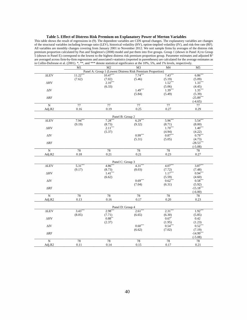
40

Table 5. Effect of Distress Risk Premium on Explanatory Power of Merton Variables This table shows the result of regressions in (9). The dependent variables are CDS spread changes. The explanatory variables are changes of the structural variables including leverage ratio (LEV), historical volatility (HV), option-implied volatility (IV), and risk-free rate (RF).

All variables are monthly changes covering from January 2001 to November 2012. We sort sample firms by averages of the distress risk

premium proportion calculated by Pan and Singleton's (2008) model and put them into five groups. Group 1 (shown in Panel A) to Group 5 (shown in Panel E) correspond to the lowest to the highest distress risk premium proportion group. Parameter estimates and adjusted R2

are averaged across firm-by-firm regressions and associated t-statistics (reported in parentheses) are calculated for the average estimates as

in Collin-Dufresne et al. (2001). *, **, and *** denote statistical significance at the 10%, 5%, and 1% levels, respectively.

M1 M2 M3 M4 M5

Panel A: Group 1 (Lowest Distress Risk Premium Proportion)

ΔLEV 11.22*** 10.47*** 7.74*** 7.43*** 6.86***

(7.62) (7.02) (5.46) (5.19) (5.09) ΔHV 2.10*** 1.52*** 1.33***

(6.33) (5.06) (4.45)

ΔIV 1.49*** 1.39*** 1.35*** (5.84) (5.49) (5.39)

ΔRF -25.89***

(-4.65)

N 77 77 77 77 77

Adj.R2 0.16 0.19 0.25 0.27 0.29

Panel B: Group 2

ΔLEV 7.94*** 7.28*** 6.29*** 5.96*** 5.54***

(9.19) (8.73) (9.32) (8.71) (8.00)

ΔHV 2.11*** 1.70*** 1.40*** (5.37) (4.94) (4.22)

ΔIV 0.99*** 0.87*** 0.79***

(5.31) (5.05) (4.73) ΔRF -28.53***

(-5.08)

N 78 78 78 78 78

Adj.R2 0.18 0.21 0.21 0.23 0.27

Panel C: Group 3

ΔLEV 5.31*** 4.86*** 4.31*** 4.07*** 3.87***

(9.17) (8.73) (8.03) (7.72) (7.48)

ΔHV 1.41*** 1.17*** 0.94***

(6.62) (5.59) (4.60)

ΔIV 0.69*** 0.62*** 0.58*** (7.04) (6.31) (5.92)

ΔRF -15.18*** (-6.00)

N 78 78 78 78 78

Adj.R2 0.13 0.16 0.17 0.20 0.23

Panel D: Group 4

ΔLEV 3.43*** 2.98*** 2.61*** 2.31*** 1.92***

(8.05) (7.71) (6.65) (6.30) (5.85)

ΔHV 0.88** 0.67* 0.42 (2.37) (1.95) (1.23)

ΔIV 0.60*** 0.54*** 0.52***

(6.62) (7.02) (7.19) ΔRF -14.99***

(-5.08)

N 78 78 78 78 78

Adj.R2 0.11 0.14 0.15 0.17 0.21

41

Panel E: Group 5 (Highest Distress Risk Premium Proportion)

ΔLEV 3.90*** 3.83*** 3.15*** 3.12*** 2.97*** (7.21) (7.33) (6.24) (6.26) (5.98)

ΔHV 1.00*** 0.84*** 0.56*

(4.37) (3.47) (1.68) ΔIV 0.50*** 0.48*** 0.44***

(4.32) (4.15) (3.83)

ΔRF -17.25*** (-6.06)

N 77 77 77 77 77

Adj.R2 0.10 0.12 0.14 0.15 0.19

42

Table 6. Effect of Distress Risk Premium on Explanatory Power of Merton Variables: Controlling

for Firm Characteristics This table reports the result of regressions in (12). The dependent variables are CDS spread changes. The explanatory variables are changes

of the structural variables including leverage ratio, historical volatility, option-implied volatility, and risk-free rate. All variables are

monthly changes covering from January 2001 to November 2012. We use 9 portfolios formed from the intersection of tercile portfolios sorted by averages of the distress risk premium proportion and each firm characteristic including leverage ratio (LEV), historical volatility

(HV), option-implied volatility (IV), Amihud’s (2002) illiquidity measure (ILLIQ), CDS liquidity (DEPTH), and credit ratings (Rating).

The distress risk premium of each firm is calculated by Pan and Singleton's (2008) model. Group 1 to Group 3 correspond to the lowest to the highest firm characteristic. For each portfolio, adjusted R2 are averaged across firm-by-firm regressions and t-statistics (reported in

bottom) are calculated from the difference of adjusted R2 between the groups with the lowest and the highest distress risk premium. *, **,

and *** denote statistical significance at the 10%, 5%, and 1% levels, respectively.

Group by Firm characteristics

DRP proportion Low Med High

Leverage ratio

Low 0.21 0.27 0.33

Med 0.21 0.25 0.27 High 0.14 0.22 0.23

L-H 0.07** 0.05* 0.10***

t-statistics (2.09) (1.49) (2.73)

Historical volatility

Low 0.22 0.29 0.30

Med 0.19 0.30 0.23

High 0.16 0.22 0.20 L-H 0.06** 0.08** 0.10***

t-statistics (2.07) (2.09) (2.59)

Implied volatility

Low 0.21 0.33 0.29 Med 0.19 0.30 0.23

High 0.18 0.20 0.20

L-H 0.04 0.13*** 0.09** t-statistics (1.28) (3.59) (2.21)

Amihud’s illiquidity

Low 0.31 0.28 0.26

Med 0.24 0.28 0.19 High 0.21 0.18 0.18

L-H 0.10*** 0.10*** 0.07**

t-statistics (2.66) (3.09) (2.02)

CDS liquidity

Low 0.18 0.34 0.33

Med 0.14 0.26 0.30 High 0.12 0.23 0.22

L-H 0.06** 0.10*** 0.11***

t-statistics (1.82) (3.18) (3.37)

Credit ratings

Low 0.27 0.28 0.30

Med 0.27 0.24 0.22

High 0.21 0.19 0.18 L-H 0.06* 0.08*** 0.11***

t-statistics (1.56) (2.68) (3.03)

43

Table 7. Test for Time-varying Effect of Distress Risk Premium on Explanatory Power of Merton

Variables: Controlling for Firm Characteristics This table reports the result of root-mean-squared errors in (11). The root-mean-squared errors are calculated from regressions in (12). The

dependent variables are CDS spread changes. The explanatory variables are changes of the structural variables including leverage ratio,

historical volatility, option-implied volatility, and risk-free rate. All variables are monthly changes covering from January 2001 to November 2012. To control firm characteristics, we sort sample firms into 9 portfolios formed from the intersection of tercile portfolios

sorted by the distress risk premium proportion and each firm characteristic at each month. The distress risk premium of each firm is

calculated by Pan and Singleton's (2008) model and the firm characteristics include leverage ratio (LEV), historical volatility (HV), option-implied volatility (IV), Amihud’s (2002) illiquidity measure (ILLIQ), CDS liquidity (Depth), and credit rating (Rating). For each time,

root-mean-squared errors are calculated from the lowest distress risk premium proportion to the highest distress risk premium proportion

group. From the time series root-mean-squared errors of the two groups, t-statistics from the difference of root-mean-squared errors are calculated for each group sorted by firm characteristics. *, **, and *** denote statistical significance at the 10%, 5%, and 1% levels,

respectively.

Group by Firm characteristics

DRP proportion Low Med High

Leverage ratio

L-H -0.27*** -0.16*** -0.17**

t-statistics (-3.15) (-2.37) (-2.04)

Historical volatility

L-H -0.23*** -0.23*** -0.15* t-statistics (-3.68) (-3.29) (-1.56)

Implied volatility

L-H -0.20*** -0.25*** -0.18**

t-statistics (-2.93) (-4.08) (-1.81)

Equity illiquidity

L-H -0.22*** -0.12** -0.10

t-statistics (-2.96) (-1.68) (-1.12)

CDS liquidity

L-H -0.12* -0.17*** -0.16** t-statistics (-1.59) (-2.41) (-2.01)

Ratings

L-H -0.17** -0.18** -0.10

t-statistics (-2.00) (-2.28) (-1.11)

44

Table 8. Cross-sectional relation between adjusted R2 and DRPs This table shows the result of cross-sectional regressions of explanatory power, measured by adjusted R2, on the average DRP proportions. We perform two-pass regressions: The first-pass (time-series) regressions are conducted firm-by-firm by either:

Level regression: 𝐶𝐷𝑆𝑖,𝑡 = 𝛽0 + 𝛽1𝐿𝐸𝑉𝑖,𝑡 + 𝛽2𝐻𝑉𝑖,𝑡 + 𝛽3𝐼𝑉𝑖,𝑡 + 𝛽4𝑅𝐹𝑡 + 휀𝑖,𝑡,

or

Change regression: Δ𝐶𝐷𝑆𝑖,𝑡 = 𝛽0 + 𝛽1Δ𝐿𝐸𝑉𝑖,𝑡 + 𝛽2Δ𝐻𝑉𝑖,𝑡 + 𝛽3Δ𝐼𝑉𝑖,𝑡 + 𝛽4Δ𝑅𝐹𝑡 + 휀𝑖,𝑡 .

Using the adjusted R2s obtained from the first-pass regressions as the dependent variable, the second-pass regression is performed by

𝑅𝑖2 = 𝛼 + 𝛽 × �̅�𝑖

𝐷𝑅𝑃 + 𝛾′𝑋𝑖 + 휀𝑖 .

Panels A and B shows the results using level regression R2s and change regression R2s as the dependent variable of the second stage,

respectively. The second stage explanatory variables are time-series averaged over the period where the each firm’s observations are

available. The cross-sectional regressions use standardized variables so that importance of each variable is comparable. *, **, and *** denote statistical significance at the 10%, 5%, and 1% levels, respectively.

M1 M2 M3 M4 M5 M6 M7 M8

Panel A. Level Regression R2

p̅DRP -0.21*** -0.21*** -0.21*** -0.21*** -0.21*** -0.21*** -0.21*** -0.17***

(-4.18) (-3.95) (-4.09) (-4.20) (-4.16) (-4.09) (-4.26) (-3.32)

Control variables

LEV 0.014 0.08 (0.28) (1.38)

HV 0.03 0.47***

(0.59) (2.87) IV -0.02 -0.30*

(-0.40) (-1.71)

ILLIQ -0.09* -0.13** (-1.78) (-2.40)

DEPTH 0.04 -0.002

(0.74) (-0.03) RATING 0.14*** 0.23***

(2.78) (3.29)

Adj. R2 0.04 0.04 0.04 0.04 0.05 0.04 0.06 0.09

Panel B. Change Regression R2

p̅DRP -0.27*** -0.20*** -0.25*** -0.25*** -0.26*** -0.23*** -0.26*** -0.16***

(-5.37) (-4.08) (-5.09) (-5.12) (-5.35) (-4.96) (-5.35) (-3.45)

Control variables LEV 0.23*** 0.16***

(4.50) (2.89)

HV 0.12** 0.24 (2.50) (1.64)

IV 0.10* -0.05

(1.95) (-0.31) ILLIQ -0.04 -0.08*

(-0.79) (-1.77)

DEPTH 0.38*** 0.40*** (8.39) (8.59)

RATING -0.06 0.02

(-1.30) (0.35)

Adj. R2 0.07 0.11 0.08 0.07 0.07 0.21 0.07 0.27

45

Table 9. Robustness Test for Effect of Distress Risk Premium on Explanatory Power of Merton

Variables This table reports the result of regressions in (12). The dependent variables are CDS spread changes. The explanatory variables are changes

of the structural variables including leverage ratio, historical volatility, option-implied volatility, and risk-free rate. All variables are

monthly changes covering from January 2001 to November 2012 (in Panel A), but the period of the Global Financial Crisis is excluded in Panel B. We use 9 portfolios formed from the intersection of tercile portfolios sorted by averages of the distress risk premium proportion

and each firm characteristic including leverage ratio (LEV), historical volatility (HV), option-implied volatility (IV), Amihud’s (2002)

illiquidity measure (ILLIQ), CDS liquidity (Depth), and credit rating (Rating). The distress risk premium of each firm is calculated either by Friewald et al.’s (2014) model (shown in Panel A) or by Pan and Singleton's (2008) model (shown in Panel B). Group 1 to Group 3

correspond to the lowest to the highest firm characteristic. For each portfolio, adjusted R2 are averaged across firm-by-firm regressions and

t-statistics (reported in bottom) are calculated from the difference of adjusted R2 between the groups with the lowest and the highest distress risk premium. *, **, and *** denote statistical significance at the 10%, 5%, and 1% levels, respectively.

Panel A: DRP by Friewald et al. (2014) Panel B: Excluding the period of GFC

DRP proportion Group by Firm characteristics

DRP proportion Group by Firm characteristics

Low Med High Low Med High

Leverage ratio Leverage ratio

Low 0.23 0.31 0.36 Low 0.19 0.25 0.25

Med 0.18 0.25 0.26 Med 0.13 0.20 0.30

High 0.15 0.18 0.22 High 0.12 0.18 0.19 L-H 0.07*** 0.13*** 0.15*** L-H 0.07** 0.07** 0.06*

t-statistic (2.41) (3.74) (4.06) t-statistic (1.94) (2.15) (1.66)

Historical volatility Historical volatility

Low 0.25 0.33 0.34 Low 0.16 0.26 0.26 Med 0.17 0.26 0.25 Med 0.12 0.24 0.25

High 0.15 0.17 0.21 High 0.14 0.17 0.17

L-H 0.10*** 0.16*** 0.12*** L-H 0.02 0.09*** 0.09*** t-statistic (3.21) (4.22) (3.40) t-statistic (0.58) (2.67) (2.45)

Implied volatility Implied volatility

Low 0.24 0.34 0.32 Low 0.17 0.29 0.24

Med 0.17 0.26 0.25 Med 0.12 0.24 0.23 High 0.16 0.17 0.20 High 0.16 0.17 0.16

L-H 0.08*** 0.16*** 0.12*** L-H 0.01 0.13*** 0.08**

t-statistic (2.94) (4.40) (3.19) t-statistic (0.31) (3.75) (2.12)

Amihud’s illiquidity Amihud’s illiquidity

Low 0.31 0.32 0.28 Low 0.27 0.24 0.21

Med 0.23 0.21 0.25 Med 0.17 0.24 0.19

High 0.17 0.21 0.17 High 0.21 0.14 0.15 L-H 0.14*** 0.11*** 0.11*** L-H 0.06** 0.10*** 0.06*

t-statistic (3.93) (3.06) (3.03) t-statistic (1.73) (3.11) (1.66)

CDS liquidity CDS liquidity

Low 0.23 0.32 0.34 Low 0.11 0.29 0.30

Med 0.15 0.27 0.25 Med 0.11 0.21 0.27

High 0.11 0.25 0.23 High 0.09 0.19 0.21 L-H 0.12*** 0.07** 0.11*** L-H 0.02 0.10*** 0.09***

t-statistic (4.11) (1.90) (2.74) t-statistic (0.73) (3.05) (2.92)

Credit rating Credit rating

Low 0.32 0.28 0.31 Low 0.23 0.24 0.25 Med 0.27 0.25 0.18 Med 0.26 0.21 0.14

High 0.19 0.17 0.19 High 0.18 0.15 0.16

L-H 0.13*** 0.12*** 0.12*** L-H 0.05 0.09*** 0.08** t-statistic (3.48) (3.77) (3.10) t-statistic (1.21) (2.94) (2.32)

46

Table 10. Robustness Test for Time-varying Effect of Distress Risk Premium on Explanatory

Power of Merton Variables This table reports the result of root-mean-squared errors in (11). The root-mean-squared errors are calculated from regressions in (12). The

dependent variables are CDS spread changes. The explanatory variables are changes of the structural variables including leverage ratio,

historical volatility, option-implied volatility, and risk-free rate. All variables are monthly changes covering from January 2001 to November 2012 (in Panel A), but the period of the Global Financial Crisis is excluded in Panel B. To control firm characteristics, we sort

sample firms into 9 portfolios formed from the intersection of tercile portfolios sorted by the distress risk premium proportion and each

firm characteristic at each month. The distress risk premium of each firm is calculated either by Friewald et al.’s (2014) model (shown in Panel A) or by Pan and Singleton's (2008) model (shown in Panel B). The firm characteristics include leverage ratio (LEV), historical

volatility (HV), option-implied volatility (IV), Amihud’s (2002) illiquidity measure (ILLIQ), CDS liquidity (Depth), and credit rating

(Rating). For each time, root-mean-squared errors are calculated from the lowest distress risk premium proportion to the highest distress risk premium proportion group. From the time series root-mean-squared errors of the two groups, t-statistics from the difference of root-

mean-squared errors are calculated for each group sorted by firm characteristics. *, **, and *** denote statistical significance at the 10%,

5%, and 1% levels, respectively.

Panel A: DRP by Friewald et al. (2014) Panel B: Excluding the period of GFC

DRP proportion Group by Firm characteristics

DRP proportion Group by Firm characteristics

Low Med High Low Med High

Leverage ratio Leverage ratio

L-H -0.22*** -0.24*** -0.35*** L-H -0.25*** -0.17** -0.17** t-statistics (-3.07) (-3.68) (-4.28) t-statistics (-2.88) (-2.22) (-2.04)

Historical volatility Historical volatility

L-H -0.18*** -0.26*** -0.33*** L-H -0.23*** -0.24*** -0.14*

t-statistics (-2.64) (-3.91) (-3.96) t-statistics (-3.80) (-3.46) (-1.45)

Implied volatility Implied volatility

L-H -0.20*** -0.21*** -0.34*** L-H -0.19*** -0.24*** -0.19**

t-statistics (-2.89) (-3.49) (-3.87) t-statistics (-2.81) (-3.78) (-1.98)

Amihud’s illiquidity Amihud’s illiquidity

L-H -0.24*** -0.25*** -0.30*** L-H -0.24*** -0.13* -0.11 t-statistics (-3.17) (-3.93) (-3.82) t-statistics (-3.29) (-1.61) (-1.16)

CDS liquidity CDS liquidity

L-H -0.24*** -0.26*** -0.32*** L-H -0.11* -0.20*** -0.19***

t-statistics (-3.12) (-3.88) (-4.31) t-statistics (-1.33) (-2.70) (-2.45)

Credit rating Credit rating

L-H -0.28*** -0.31*** -0.21*** L-H -0.14* -0.19** -0.14**

t-statistics (-3.31) (-4.56) (-2.46) t-statistics (-1.51) (-2.26) (-1.71)

47

0 0.2 0.4 0.6 0.8 10

100

200

300

400

500

600

700

800

CD

S s

pre

ad

(b

ps)

DP=0.15

DP=0.10

DP=0.05

Figure 1. The model spreads of a CDS

This figure shows the relationship between the variation level of the default intensity process, 𝜎, and the CDS spread. The default intensity

follows the lognormal process in equation (3) and the CDS spread is calculated by equation (16) with five-year maturity. We set the current

default intensity, 𝜆𝑡𝑄

, and the parameters for the market price of risk, 𝛿0 and 𝛿1, to 0.005, -2.906, and -0.619, respectively. The parameter

of the mean-reversion rate under the physical measure, 𝜅𝑃, is fixed to 0.637 and the long-term mean parameter, 𝜃𝑃, is adjusted to hold constant the default probability to 0.05, 0.10, and 0.15.

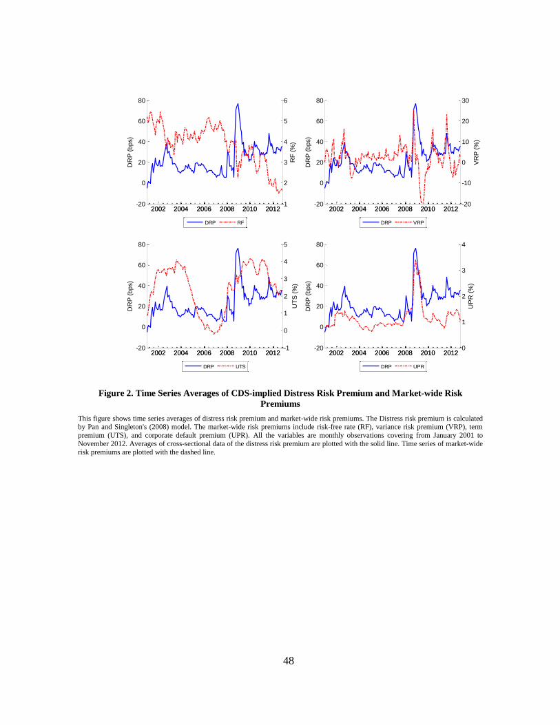
48

Figure 2. Time Series Averages of CDS-implied Distress Risk Premium and Market-wide Risk

Premiums

This figure shows time series averages of distress risk premium and market-wide risk premiums. The Distress risk premium is calculated by Pan and Singleton's (2008) model. The market-wide risk premiums include risk-free rate (RF), variance risk premium (VRP), term

premium (UTS), and corporate default premium (UPR). All the variables are monthly observations covering from January 2001 to November 2012. Averages of cross-sectional data of the distress risk premium are plotted with the solid line. Time series of market-wide

risk premiums are plotted with the dashed line.

2002 2004 2006 2008 2010 2012-20

0

20

40

60

80

DR

P (

bp

s)

2002 2004 2006 2008 2010 20121

2

3

4

5

6

RF

(%

)

DRP RF

2002 2004 2006 2008 2010 2012-20

0

20

40

60

80

DR

P (

bp

s)

2002 2004 2006 2008 2010 2012-20

-10

0

10

20

30

VR

P (

%)

DRP VRP

2002 2004 2006 2008 2010 2012-20

0

20

40

60

80

DR

P (

bp

s)

2002 2004 2006 2008 2010 2012-1

0

1

2

3

4

5

UT

S (

%)

DRP UTS

2002 2004 2006 2008 2010 2012-20

0

20

40

60

80

DR

P (

bp

s)

2002 2004 2006 2008 2010 20120

1

2

3

4

UP

R (

%)

DRP UPR

49

Figure 3. Time Series Averages of CDS-implied Distress Risk Premium Proportion and Market-wide

Risk Premiums

This figure shows time series averages of distress risk premium proportion and market-wide risk premiums. The Distress risk premium is calculated by Pan and Singleton's (2008) model. The market-wide risk premiums include risk-free rate (RF), variance risk premium (VRP),

term premium (UTS), and corporate default premium (UPR). All the variables are monthly observations covering from January 2001 to November 2012. Averages of cross-sectional data of the distress risk premium proportion are plotted with the solid line. Time series of

market-wide risk premiums are plotted with the dashed line.

2002 2004 2006 2008 2010 2012-10

0

10

20

30

40

DR

P p

rop

ort

ion

(%

)

2002 2004 2006 2008 2010 20121

2

3

4

5

6

RF

(%

)

DRP proportion RF

2002 2004 2006 2008 2010 2012-10

0

10

20

30

40

DR

P p

rop

ort

ion

(%

)

2002 2004 2006 2008 2010 2012-20

-10

0

10

20

30

VR

P (

%)

DRP proportion VRP

2002 2004 2006 2008 2010 2012-10

0

10

20

30

40

DR

P p

rop

ort

ion

(%

)

2002 2004 2006 2008 2010 2012-1

0

1

2

3

4

5

UT

S (

%)

DRP proportion UTS

2002 2004 2006 2008 2010 2012-10

0

10

20

30

40

DR

P p

rop

ort

ion

(%

)

2002 2004 2006 2008 2010 20120

1

2

3

4

UP

R (

%)

DRP proportion UPR

50

Figure 4. Explanatory Power Change of Merton Variables by Distress Risk Premium

This figure shows adjusted R-square changes from regressions in (8) and (9). The regressions are performed on both levels (shown on the left) and changes (shown on the right). The dependent variables are CDS spreads and the explanatory variables are the structural variables

including leverage ratio, historical volatility, option-implied volatility, and risk-free rate. All variables are monthly observations covering

from January 2001 to November 2012. We sort sample firms by averages of the distress risk premium proportion calculated by Pan and Singleton's (2008) model and put them into five groups. Group 1 to Group 5 correspond to the lowest to the highest distress risk premium

proportion group. Adjusted R2 are averaged across firm-by-firm regressions.

Low 2 3 4 High20

30

40

50

60

70

80

DRP Proportion

Ad

juste

d R

2 (

%)

M1 M2 M3 M4 M5

Low 2 3 4 High5

10

15

20

25

30

DRP Proportion

Ad

juste

d R

2 (

%)

M1 M2 M3 M4 M5