Eleventh USA/Europe Air Traffic Management Research and Development Seminar (ATM2015)

The current practice of separation delivery

at major European airports

Gerben van Baren

Air Transport Safety Institute

National Aerospace Laboratory - NLR

Amsterdam, The Netherlands

vanbaren@nlr-atsi.nl

Catherine Chalon-Morgan, Vincent Treve

Airport Research Unit, D-ATM

EUROCONTROL

Brussels, Belgium

vincent.treve@eurocontrol.int

Abstract— Separation minima are or can become a key

bottleneck for the runway throughput at major airports.

Therefore, in the context of SESAR Project 6.8.1,

EUROCONTROL is investigating concepts for flexible and

dynamic use of wake turbulence separations. In order to

successfully develop such concepts and optimize the benefits, it is

important that current practices and lessons learnt from today’s

operations are understood and taken into account. The aim of the

study presented in this paper is therefore to baseline the current

practices for separation delivery on final approach at major

European airports. For this, site visits to European ATC units in

combination with analysis of radar data have been conducted.

Statistical characteristics on speed, distance and time spacing as

observed in today’s operations depending on e.g., airport,

headwind, and distance to threshold are determined. Distance

spacing close to the threshold as observed in the data satisfies the

minimum radar or wake turbulence separation minima with a

buffer that is on average in between 0.5 and 1.0 NM and has a

standard deviation of about 0.5 NM. The mean compression of

distance spacing on the last 10 NM of the final approach is

approximately 1 NM. About half of this compression occurs when

the leader aircraft is beyond 4 DME when aircraft adapt to their

final approach speed. It is shown that there are considerable

differences per airport, and this illustrates that it is important to

take into account local conditions in the assessment of benefits for

a certain airport. Furthermore, the observed mean and variation

of spacing buffers may suggest that for optimized runway

throughput, new concepts should not only focus on reduction of

minima but also on the management of distance spacing

compression variation, e.g. better understanding and predicting

aircraft speed performance, such that buffers can be optimized.

The results of this study are used by SESAR and

EUROCONTROL in the development of a new ATC tool to

predict aircraft speed performance. This Leading Optimised

Runway Delivery (LORD) tool supports Air Traffic Controllers

to optimize the separation buffer and more efficiently and easily

deal with the compression effect on the last part of the final

approach.

Wake turbulence separation, minimum separation, speed

control, separation management

I. INTRODUCTION

In today’s operations, a limiting factor for runway throughput is the required minimum separation. This is either a minimum radar separation or a wake turbulence separation. The latter is based on ICAO’s definition of wake turbulence categories and minima, sometimes with local adaptations. SESAR Project 6.8.1 investigates concepts for the flexible and dynamic use of wake turbulence separations that could replace the static and to some extent suboptimal ICAO Wake Turbulence (WT) classification scheme. This includes concepts such as Time Based Separation (TBS, see e.g., [1]), Pairwise separation (PWS) and conditional reduction of wake separation as a function of weather conditions. These concepts may be operated individually or in combination.

In order to ensure that such new concepts bring the expected benefits, it is important that current practices and lessons learnt from today’s operations are taken into account, in particular the busiest operations at major airports. This way, the benefits for European stakeholders can be optimized. Therefore, in the context of SESAR Project 6.8.1, EUROCONTROL launched the ‘Optimised Runway Delivery study’.

To obtain the required understanding of the current practices, information on operational experience has been collected through site visits to six major European airports: Barcelona El Prat, London Gatwick, London Heathrow, Milan Malpensa, Paris Charles de Gaulle, and Vienna Schwechat. These are all airports in the Top 30 with respect to arrival ATFM delay as described in EUROCONTROL’s Performance Review Report 2013 [2]. The working practice of TWR and APP controllers has been observed and operational controllers have been interviewed. Furthermore, radar data of approach operations to these airports has been collected and analyzed with respect to ground speed, and distance and time spacing and has been correlated to weather data with a focus on headwind conditions.

In the following, the current practice is described as observed in the site visits and in the radar data analysis. First, a

This work was funded by the SESAR Project 6.8.1

description of the flight data set and the analysis method is given.

II. FLIGHT DATA SET DESCRIPTION AND ANALYSIS METHOD

Radar data has been provided by the Air Navigation Service Providers (ANSPs) for four of the six visited airports. For one other airport, ADS-B data has been used. The radar data sets per airport cover at least several months of data in 2012 and 2013. The ADS-B data set is smaller covering two weeks of data in 2013. In total, the data set counts about 130,000 flights.

For each flight, time, lateral and longitudinal position coordinates, altitude (sometimes in feet, sometimes in flight levels), ground speed, and aircraft type are available.

The position data has been converted to distance to threshold. For this, the coordinates of the runway thresholds have been used. The runway concerned for a certain track – if not available in the data – is determined based on course of the track and the distance of the track points to the runway threshold.

As the focus of this project is on the delivery of separation to aircraft on final approach, where the approach path follows the extended runway centerline, the data per flight is limited to the last 20 NM before the runway threshold and only flights for which these data points are complete are taken into account.

The analysis is focused on determining the evolution of ground speed, distance and time spacing along the final approach, from glide path interception down to passing the runway threshold.

Ground speed is directly available in the data set. The spacing in nautical miles (NM) or seconds (s) at a certain position on the final approach path is determined as the spacing behind an aircraft to its successor: spacing is looked at from the perspective of the leader aircraft.

To focus on relatively high traffic density situations, those flights are selected where 3 or more aircraft are simultaneously within the last 10 NM of the final approach. The distribution of how many aircraft are within the last 10 NM at each airport (referred to as APT1 to APT5) is shown in Figure 1. The number is in between 1 and 4. The percentage of flights with 3 or more aircraft within 10 NM on final is an indication of the overall traffic pressure at the airport. The figure shows that traffic pressure is highest at airport 4 and lowest at airport 3, where respectively for 74% and 13% of the flights there are 3 or more aircraft within 10 NM (see also Table I). The relatively low percentage of for airport 5 is due to a high percentage of mixed mode operations with departure gap spacing.

Furthermore, only flights of aircraft types in the ICAO Heavy or Medium WTC have been considered. Applying the abovementioned selection criteria, about 50,000 flights have been used for analysis (see Table I). All graphs shown in the following are based on this set of data.

Given the type of the leader and follower aircraft and their wake turbulence category, the applicable separation minimum can be determined. The percentage of occurrence of aircraft

types in the traffic mix per airport is shown in Figure 2 for the 43 most frequently occurring types in the ICAO Wake Turbulence Categories (WTC). It is to be noted that for UK airports, another classification is used, which is introduced in section III.C. Obviously, aircraft types of the A320-family are dominant. Regarding WTC, this implies that the dominant combination is Medium behind Medium. For the airports investigated this is in the order of 80 to 90% in the selected data set.

TABLE I. NUMBER OF FLIGHTS IN THE DATA SET

Airport APT1 APT2 APT3 APT4 APT5

Total number of

flights 28,395 35,724 2,524 36,921 25,521

Selected number of

flights 7,128 10,631 315 25,650 4,046

Percentage of

flights selected 25 30 12 69 16

To analyze the difference between actual spacing as observed in the radar data and the related separation minimum, the spacing buffer is defined as the distance in NM between actual spacing at a certain point and the separation minimum. The use of spacing buffer as a metric instead of absolute distance spacing facilitates to compare airports that apply different WTC and separation minima and also – to some extent – filters out the effect of different traffic mixes.

Figure 1 – Percentage of occurrence of number of aircraft

within last 10 NM (either 1, 2, 3 or 4)

Figure 2 – Percentage of occurrence of aircraft types in the traffic mix per

airport (25 most frequently occurring Heavy and Medium types)

In addition to the flight data, weather data has been collected. In the current study, publicly available METAR data is used including wind speed and direction at the runway surface, gust, and visibility information. It is to be noted that the runway surface headwind can be considerably different from the headwind as experienced on the glide slope. For the current study only data on runway surface headwind has been used. For each flight, the METAR closest in time to the runway threshold passage time is used. Distribution of the runway surface headwind and visibility conditions as experienced by the flights in the data set is shown in Figure 3 and 4. In Figure 3, the colors refer to intervals of headwind strength in kts, as explained in the legend. Runway surface headwind predominantly (for more than 50% of the time) is in between 0 and 10 kts. Stronger headwind above 10 kts occurs most frequently (25%) at airport 2. For the other airports this is less than 20%. Regarding visibility as presented in Figure 4, it is shown that for more than 65% of the time at all airports, visibility exceeds 6 NM. Visibility below 1 NM occurs in maximum 5% (airport 3) of the time.

III. DESCRIPTION OF THE CURRENT PRACTICE

A. Introduction

The current practice is described distinguishing the following

aspects: process from entering the Terminal Maneuvering

Area (TMA) to touchdown, speed control, separation minima,

separation assurance, and compression and pull away. For

each of these aspects, the information from the site visits and

data analysis is discussed in combination.

B. Process from entering TMA to touchdown

An aircraft approaching an aerodrome typically follows a Standard Arrival Route (STAR) providing the transition from the en-route structure to the flow for the active landing runway. Aircraft from different directions may use different STARs which are then merged into a single flow.

Within the TMA, the aircraft is controlled by one or more approach (APP) controllers, dependent on the traffic density and the number of directions aircraft can come from. The names of these controllers and their distribution of tasks may vary from unit to unit. E.g., there may be an initial controller (INI), an intermediate controller (INT) or feeder, and final controller (FIN) or director. The FIN transfers the aircraft to the tower (TWR) or runway controller.

A typical distribution of the approach segments over the positions is sketched in Figure 6 with indications of the Initial Approach Fix (IAF) and Final Approach Point (FAP).

Regarding transfer from approach to the tower, distinction can be made between hand-over of communication and transfer of control. Transfer of control and thus transfer of responsibility for separation usually is at 4 DME

1, although

there are examples where it is 6 or 8 DME. In these latter cases the tower controller may also be qualified as radar controller.

Transfer of communication from APP to TWR is normally before the transfer of control and usually is a silent hand-over which takes place between 10 and 6 DME and not later than 4 DME before the runway threshold. In a silent hand-over the APP controller instructs the flight crew to change frequency to the TWR and then to contact the TWR; there is no communication required between APP and TWR. This typically occurs when the aircraft is established on the glide slope, has adopted the instructed speed and is sufficiently separated.

The point where aircraft intercept the localizer can vary considerably from runway to runway and further depend on ATC practices and traffic density. The altitude to which aircraft level off before glide slope interception varies as well, roughly between 1500 and 4500 ft (assuming a 3 degrees glide slope angle) above the altitude of the runway threshold. As a consequence, the location of the FAP, the point where the aircraft intercepts the glide slope, varies roughly between 5 and 14 DME before the threshold.

Figure 5 shows the mean altitude profiles as observed in the data per airport. The altitude profiles converge to a 3 degrees glide slope path on the last 8 NM. Differences in altitude profiles before 8 DME are caused by different ATC practices, different locations of the FAP and accordingly differences in intercept altitudes. It is to be noted that per airport, data of flights to various runways, with different FAP locations is included.

1 Distance to threshold is denoted here in DME in order to

avoid confusion with distance spacing expressed in NM.

Figure 4 – Percentage of occurrence of visibility conditions per airport

Figure 3 – Percentage of occurrence of runway surface headwind

conditions per airport

C. Speed control

Speed control, where ATC instructs the aircraft to fly a certain Indicated Air Speed (IAS) at a certain segment of the approach, is defined and described in the Aeronautical Information Publication (AIP) at many airports.

The speed control as described for the visited airports appears to be quite similar. It typically starts with 210/220 kts on downwind, 180 kts is to be expected from baseleg to localizer interception or from localizer interception to glide slope interception, then reducing to 160 kts until 4 DME. Afterwards, the aircraft adopts its Final Approach Speed (FAS). The speeds at the various segments are sketched in Figure 6. Because of differences in Final Approach Points, the length of the segments where a certain speed is controlled may vary.

To what extent the speed control is actually applied may be subject to the traffic density or other conditions. And even when speed control is applied, there can still be considerable variation in the actual distribution of speed, both indicated airspeed (IAS) and ground speed. Variation in IAS is impacted by a number of factors. It depends on the timing of when the controller issues a speed instruction, which is influenced on the initial spacing set up and whether there is a need to intervene through speed control because of a developing separation infringement scenario. Furthermore, the adaptation of an instructed speed may take time: the flight crew has to act and depending on the Flight Management System (FMS) of the

aircraft, the time it takes to reach the instructed speed can vary as well. Given a certain IAS, the resulting ground speed is affected by the headwind along the glide slope. Figure 7 shows the mean ground speed profiles per airport. The plot shows considerable differences up to 30 kts in mean speed over the airports, in particular before 4 DME from the threshold. Beyond 4 DME, the ground speed curves converge to a common mean value in accordance with the Final Approach Speed of aircraft.

There can be considerable variation around the mean value, because of differences in aircraft type, traffic mix, landing weight, stabilization altitude, stabilization mode, weather conditions, and the associated airline operator cockpit procedures. The range of FAS varies from under 100 kts for some Light wake category aircraft types to over 160 kts for some Heavy wake category aircraft types. Even for a particular aircraft type, the variation in FAS may be ± 20 kts, e.g., because of variations in actual landing weight and weather, and the actual FAS is usually not known to ATC. Figure 8 shows the distribution of ground speed at 2 DME before the runway threshold for aircraft types DH8D, A320, and B744 as observed in the data. On top of the histograms, the mean and 5

th and 95

th percentile are indicated. Although there are

differences between FAS and resulting ground speed the figure illustrates the substantial variation in speed for a certain aircraft type as well as between different aircraft types.

Figure 8 – Distribution of ground speed at 2 DME for

three different aircraft types

FAP

IAF

180 kts

4 NM

Figure 6 - Sketch of typical distribution of approach segments

between controller positions and generic speed control procedure

Figure 7 – Mean ground speed profiles per airport

Figure 5 – Mean altitude profiles per airport

Figure 9 shows the variation in ground speed for data of all airports together on the last 10 NM of the approach. In addition to the mean value, the 5

th and 95

th percentile and the mean ±

the standard deviation are shown. The variation as observed is ± 30 kts at 10 DME, decreasing to ±15 kts on the segment after 4 DME down to threshold. The standard deviation is in the order of 20 kts at 10 DME decreasing to 10 kts close to the threshold.

Variation in ground speed per airport is shown in Figure 10. In this figure, each row represents a location along the approach path (at 10, 7, 4 and 0.5 NM before the runway threshold). The first column represents data of all airports together and the following columns each represent an airport. The vertical bars indicate the 5

th to 95

th percentile interval. The

marker indicates the mean value. The label next to the marker lists the mean (µ) and standard deviation (σ) value. The figure shows differences in mean as already shown in Figure 7 and also differences in variation. Standard deviation is highest at airport 2, starting at 26 kts and decreasing to 10 kts, and lowest at airport 4, starting at 16 kts and decreasing to 10 kts.

Figure 11 presents similar information on mean and variation per headwind condition. A headwind condition is defined as a 5 kts interval, e.g., from 0 to 5 kts, from 5 to 10

kts, etc. The figure clearly shows the effect of headwind on mean ground speed. The mean ground speed roughly decreases with the same amount as the headwind increases, but drops more steeply in headwinds above 15 kts. One can also observe that the standard deviation is quite constant over the headwind conditions, around 20 kts at 10 DME down to 9 kts at 0.5 DME.

D. Separation minima

For safely separating approaching aircraft, in addition to Minimum Radar Separation (MRS), WT separation is considered. Default MRS is 3.0 NM and most airports have specified conditions where and when 2.5 NM is allowed on final. Such conditions are defined in terms of weather (visibility) conditions, runway conditions, and the WTC of the involved aircraft and can be applied up to a distance varying between 10 and 20 NM before the runway threshold.

WT separations predominantly follow ICAO WTC and minima (Table II, [3]), with some local adaptations for specific aircraft types like B777, B757 or turbo props, and except for UK airports where the UK six categories and associated minima (Table III, [4]) are applied.

Visual separation is allowed in certain specified conditions at many airports and is used as a way to relieve MRS and WT separation minima. Distinction is to be made between visual separation by the TWR controller and by the flight crew. In the first case, the TWR controller should have both aircraft in sight and the required visibility conditions vary from airport to airport, from at least 4 NM to 6.5 NM. In the latter case, the controller asks the flight crew to maintain own separation from the preceding aircraft. It can also occur that the flight crew asks permission to maintain own separation.

E. Separation assurance

Given the approach path, the speed control applied and the wind conditions, the resulting ground speed profile of two succeeding aircraft determines how the spacing develops on the final approach in view of the separation criteria.

Figure 11 – Evolution of ground speed per headwind condition, showing mean,

5th and 95th percentile and standard deviation, at 10, 7, 4, and 0.5 NM

before the runway threshold

Figure 10 – Evolution of ground speed per airport, showing mean, 5th and 95th

percentile and standard deviation, at 10, 7, 4, and 0.5 NM

before the runway threshold

Figure 9 – Ground speed profile of all airports together, showing mean, 5th and

95th percentile and standard deviation

TABLE II. ICAO WTC AND MINIMA IN NM ([3])

Leader

WTC

Follower WTC

Super Heavy Medium Light

Super 6 7 8

Heavy 4 5 6

Medium 5

Light

TABLE III. UK WTC AND MINIMA IN NM ([4])

Leader

WTC

Follower WTC

Super Heavy Upper

Medium

Lower

Medium Small Light

Super 6 7 7 7 8

Heavy 4 5 5 6 7

Upper

Medium 3 4 4 6

Lower

Medium 3 5

Small 3 4

Light

Based on experience, the approach controller(s) will set up the initial spacing before localizer interception, taking into account the abovementioned factors, the traffic density conditions and the applicable minimum radar or wake turbulence separation. Initial spacing applied between two arriving aircraft is generally about 5 NM, or 10 NM in case of two traffic flows. To the extent possible sequencing takes into account WT categories, in order to group Heavies.

The approach controllers mainly use vectoring and speed control as instruments to establish and maintain separation. A small or temporary loss of separation can be tolerated, e.g., when it is caused by a sudden change of wind that is resolved quickly afterwards.

Regarding the point of delivery, the point until where the required separation minimum should be satisfied, there are two main procedures: delivery to threshold (most common) and delivery to 4 DME. Note that in both cases, ATC is responsible for separation to threshold. In the latter case, WT separation minima are applied at 4 DME, taking into account compression after 4 DME.

Generally speaking, separation assurance is the responsibility of the APP controller. The TWR controller has only few options to directly manage separation and will when necessary coordinate with the APP controller. However, in some ATC units the TWR controller has responsibility already from 6 or 8 DME before the threshold and has a radar rating. To resolve a potential loss of separation, the first option considered is to reduce the airspeed of the follower aircraft. When this is judged as not being sufficient, or when this is not possible because of the follower has a high FAS, other options such as path stretching can be considered if the situation permits. In exceptional cases and when the runway configuration allows it may be possible to switch the follower

to a parallel runway as long as the aircraft has sufficient time to establish and stabilize again. An option for the TWR controller is to apply or offer the aircraft visual separation (provided VMC applies) to relieve the radar or WT separation minimum. If no other option is available the controller can instruct the follower aircraft a go-around.

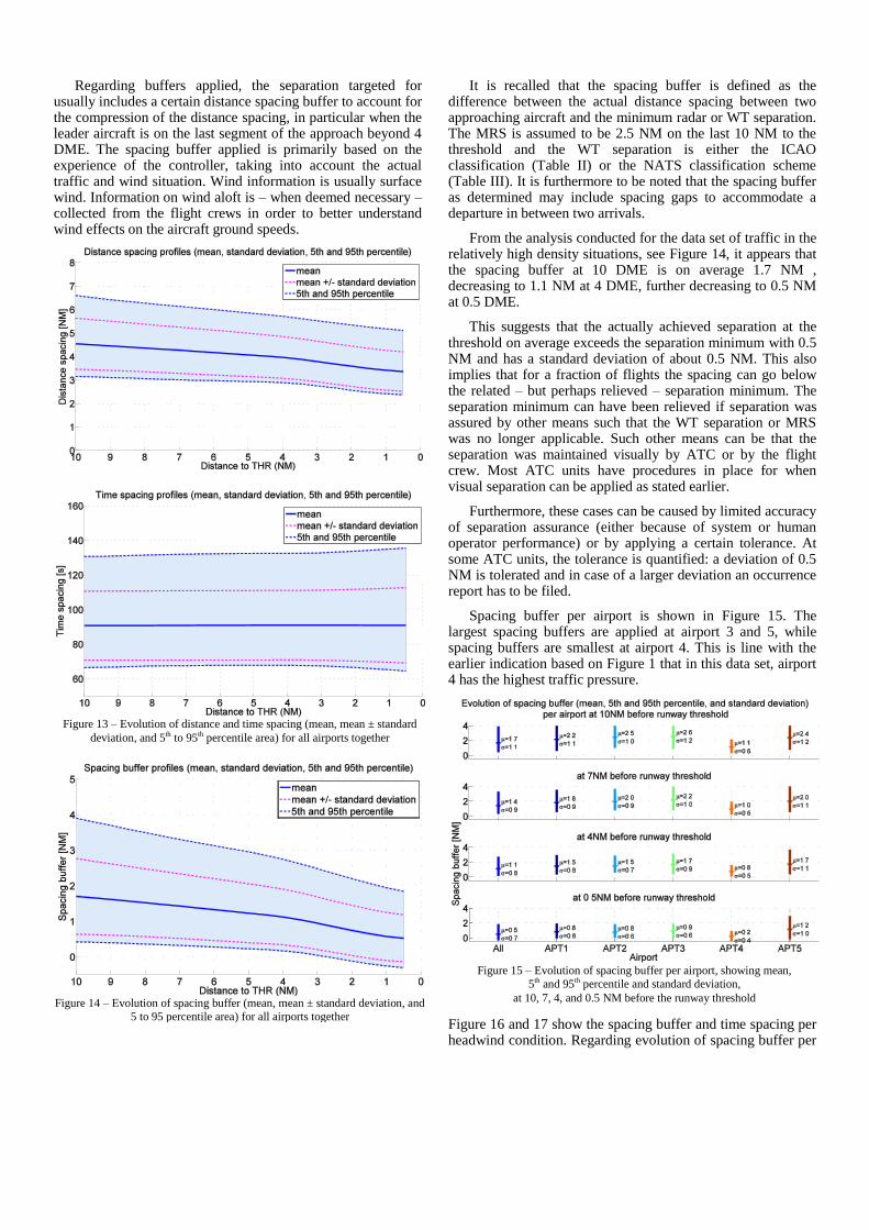
The mean distance and time spacing as observed in the data is shown in Figure 12. For all airports, there is a slightly decreasing trend of mean distance spacing towards the threshold. This is the distance compression effect because of the follower aircraft having a ground speed higher than the leader aircraft. Time spacing appears to be rather constant with decreasing distance to threshold. Obviously, lower mean value of distance spacing (e.g., orange curve for airport 4) results in lower mean time spacing. Apparently, mean spacing can vary considerably over the airports, up to 1 NM or 20 seconds. This can be explained by differences in traffic mix, differences in applied wake turbulence categories and minima, and/or differences in buffers applied.

In addition to the variations in mean spacing per airport, there is variation around the mean, as shown for the data of all airports together in Figure 13. The distance spacing (top plot) can vary (5

th to 95

th percentile) between 3 and 7 NM at 10

DME and between 2.5 and 5.5 NM at 0.5 DME. The overall variation in time spacing (bottom plot) is in the order of 60 seconds.

Figure 12 – Evolution of mean distance and time spacing per airport

Regarding buffers applied, the separation targeted for usually includes a certain distance spacing buffer to account for the compression of the distance spacing, in particular when the leader aircraft is on the last segment of the approach beyond 4 DME. The spacing buffer applied is primarily based on the experience of the controller, taking into account the actual traffic and wind situation. Wind information is usually surface wind. Information on wind aloft is – when deemed necessary – collected from the flight crews in order to better understand wind effects on the aircraft ground speeds.

It is recalled that the spacing buffer is defined as the difference between the actual distance spacing between two approaching aircraft and the minimum radar or WT separation. The MRS is assumed to be 2.5 NM on the last 10 NM to the threshold and the WT separation is either the ICAO classification (Table II) or the NATS classification scheme (Table III). It is furthermore to be noted that the spacing buffer as determined may include spacing gaps to accommodate a departure in between two arrivals.

From the analysis conducted for the data set of traffic in the relatively high density situations, see Figure 14, it appears that the spacing buffer at 10 DME is on average 1.7 NM , decreasing to 1.1 NM at 4 DME, further decreasing to 0.5 NM at 0.5 DME.

This suggests that the actually achieved separation at the threshold on average exceeds the separation minimum with 0.5 NM and has a standard deviation of about 0.5 NM. This also implies that for a fraction of flights the spacing can go below the related – but perhaps relieved – separation minimum. The separation minimum can have been relieved if separation was assured by other means such that the WT separation or MRS was no longer applicable. Such other means can be that the separation was maintained visually by ATC or by the flight crew. Most ATC units have procedures in place for when visual separation can be applied as stated earlier.

Furthermore, these cases can be caused by limited accuracy of separation assurance (either because of system or human operator performance) or by applying a certain tolerance. At some ATC units, the tolerance is quantified: a deviation of 0.5 NM is tolerated and in case of a larger deviation an occurrence report has to be filed.

Spacing buffer per airport is shown in Figure 15. The largest spacing buffers are applied at airport 3 and 5, while spacing buffers are smallest at airport 4. This is line with the earlier indication based on Figure 1 that in this data set, airport 4 has the highest traffic pressure.

Figure 16 and 17 show the spacing buffer and time spacing per headwind condition. Regarding evolution of spacing buffer per

Figure 15 – Evolution of spacing buffer per airport, showing mean,

5th and 95th percentile and standard deviation,

at 10, 7, 4, and 0.5 NM before the runway threshold

Figure 14 – Evolution of spacing buffer (mean, mean ± standard deviation, and

5 to 95 percentile area) for all airports together

Figure 13 – Evolution of distance and time spacing (mean, mean ± standard

deviation, and 5th to 95th percentile area) for all airports together

headwind conditions, there are no significant differences observed. For time spacing both the mean and standard deviation appear to increase with headwind. For headwind up to 15 kts, the increase in time spacing appears limited to about 1 second per 5 kts increase of headwind. For stronger headwind, the observed increase is larger, in the order of 8 seconds. This is in line with the observed differences in ground speed per headwind conditions in Figure 11.

For visibility conditions, it is interesting to see in Figure 18 that for visibility in between 0 and 1 NM, the spacing buffer is about 0.5 NM larger than in the other visibility conditions. It is to be noted that this observation is based on a limited number of flights, because these conditions only concern less than 1% of the analyzed flights. Nevertheless, this larger spacing buffer can be caused by procedural reduction of runway throughput and increased separation minima in low visibility (Low Visibility Procedures or LVP). It is to be noted that these increased separation minima have not been taken into account in determining the spacing buffer. Furthermore, it can be an indication that spacings less than the MRS or WT minima,

using visual separation instead, are applied in good visibility conditions only.

F. Compression and pull away

In general, distance spacing tends to reduce during the final approach phase. This demonstrates the compression effect because of the reduction of speed between interception and touchdown. There can however be wind conditions evolving along the glide slope that result in (temporarily) increasing distance spacing.

The compression is visualized in Figure 19 for the mean of the spacing buffer distinguishing three segments of the approach: from 10 to 7 DME before threshold, from 7 to 4 DME, and from 4 to 0.5 DME. For example, looking at the first column in Figure 19, representing data of all airports together, the mean buffer at 10 DME is 1.7 NM, then reduces to 1.4 NM at 7 DME, further reduces to 1.1 NM at 4 DME and to 0.5 NM at 0.5 DME before the threshold. Overall, the mean spacing between 10 and 0.5 DME has thus reduced by 1.2 NM and half (0.6 NM) of this total compression occurs when the leader aircraft is beyond 4 DME. The most compression is observed at airports 2 and 3 and the least compression at airport 4.

Compression in the first phase, covering glide slope interception down to 4 DME, is relatively predictable as the speed variations are coherent for all aircraft and dictated by the procedural speed control. Time spacing is rather constant in this phase, as can be seen in Figure 20, showing the compression of time spacing per airport. The least compression observed for airport 4 in Figure 19, may be the result of relatively strict application and adherence to speed control procedures. As stated earlier, airport 4 has the highest traffic pressure in this data set and for airports 2 and 3 with lower traffic pressure, spacing buffers can be larger and compression is then less of an issue.

Figure 18 – Evolution of spacing buffer per visibility condition, showing mean,

5th and 95th percentile and standard deviation ,

at 10, 7, 4, and 0.5 NM before the runway threshold

Figure 17 – Evolution of time spacing per headwind condition, showing mean,

5th and 95th percentile and standard deviation,

at 10, 7, 4, and 0.5 NM before the runway threshold

Figure 16 – Evolution of spacing buffer per headwind condition, showing

mean, 5th and 95th percentile and standard deviation,

at 10, 7, 4, and 0.5 NM before the runway threshold

In the second phase, beyond 4 DME, the spacing distances continue to reduce but in different proportions as a function of the leader and follower Final Approach Speeds. The time spacings may vary significantly in this phase. The follower is gaining or loosing time compared to the leading aircraft. At the first order, the time lost or gained is driven by the Final Approach Speeds of the leader and follower and therefore by the pair of aircraft types. This is illustrated in Figure 21 and Figure 22 for combinations of B744, A320, and DH8D for compression of spacing buffer and time spacing respectively.

In Figure 21, the compression of the spacing buffer is presented. The plot e.g., shows that for B744 behind B744, there is on average a reduction in mean spacing buffer of 0.7 NM. At 10 DME, the mean spacing buffer is 0.8 NM and reduces to 0.2 NM at 0.5 DME. The associated time spacing as shown in Figure 22 hardly changes (0.6 seconds) for B744 behind B744.

For A320 behind B744, the mean spacing also reduces by 0.7 NM, while the time spacing increases by about 10 s. This demonstrates the ‘pull away’ effect when the FAS of the follower aircraft (in this case the A320) is lower than that of the leader aircraft (the B744), see also Figure 8.

For DH8D behind A320 or vice versa, compression of distance spacing is for both 1.7 NM, while time spacing increases by about 5 s when the DH8D is follower and decreases by about 5 s when the A320 is follower. This is

because the mean FAS of the DH8D is slower than the mean FAS of the A320, see also Figure 8.

IV. CONCLUDING REMARKS

Regarding the current practices for separation delivery, there are commonalities – partly obvious because of the common ICAO standards and regulations that are adhered to – e.g., the use of separation minima, the organization of controller tasks, the use of speed control, and the use of tools to visualize, monitor and manage separation and related (speed, weather) information.

There are furthermore obvious airport dependencies, such as runway use modes, approach procedures, location of FAP and glide path interception altitude, weather conditions, traffic mix and traffic pressure.

In addition, differences have been observed, e.g., in the point of separation delivery, exceptions on separation minima for particular aircraft types, the use of visual separation in certain conditions, and the way potential separation infringements are dealt with.

Other factors that are expected to have a substantial influence on the resulting spacing, but are more difficult to

Figure 20 – Compression of mean time spacing per airport at three segments

Figure 22 – Compression of mean time spacing for certain aircraft

combinations at three segments

Figure 21 – Compression of mean spacing buffer for certain aircraft

combinations at three segments

Figure 19 – Compression of mean spacing buffer per airport at three segments

analyze are differences in individual controllers’ practices, differences in airline and flight crew practices and in actual aircraft weight.

The radar data analysis has shown the effect of certain of the abovementioned parameters on the speed and spacing. Overall, distance spacing as observed satisfies the (MRS and WT) separation minima with a buffer that is close to the threshold (analyzed at 0.5 DME) on average in between 0.5 and 1.0 NM. The variability in spacing buffer has a standard deviation of about 0.5 NM and this variability is rather common over all airports, runways, combinations of WT categories, headwind and visibility conditions.

One effect observed is the effect of headwind: With increasing headwind, the ground speed decreases and – in consequence – the time spacing increases. It can also be observed that the spacing buffer applied hardly varies with headwind.

For a percentage of the data, the distance spacing observed is below the related MRS or WT separation minimum. These cases can be (partly) because of application of visual separation by ATC or flight crew, inaccuracies or (temporarily) tolerated reductions in separation, but the data could not be analyzed with respect to these parameters.

Considering all data, the amount of distance compression on the final approach from 10 DME to 0.5 DME before threshold is approximately 1 NM. About half of this total compression occurs when the leader aircraft is beyond 4 DME. Distance compression appears rather insensitive to runway surface headwind and visibility conditions. Looking at differences between airports, compression from 10 to 0.5 DME varies between 0.9 NM to 1.7 NM.

The results of this study, being a description of the baseline while also indicating the local variations can be used in the further development and validation of separation concepts. The differences in results per airport illustrate that it is furthermore important to take into account local conditions in the assessment of benefits for a certain airport.

The observed variation in speed and spacing with mean spacing buffers of 0.5 NM or more may suggest that for optimized runway throughput, new concepts should not only focus on reduction of minima but also on the management of distance spacing compression variation. Better understanding and predicting aircraft speed performance will enhance predictability of operations, such that buffers can be optimized. For this, more detailed information on weather and aircraft performance may be needed.

The results of this study are used as an input by SESAR and EUROCONTROL in the development of a new ATC tool to predict aircraft speed performance. This Leading Optimized Runway Delivery (LORD) tool supports Air Traffic Controller to optimize the separation the buffer and more efficiently and easily deal with the compression effect on the last part of the final approach. Real-time simulations have already shown that for delivering separation minima at threshold, a better prediction of the required separation buffer can reduce the rate of under-spaced pairs while increasing runway throughput. This is especially true in adverse wind conditions, like tailwind

at interception and headwind at threshold, when delivering separation accurately is more difficult.

ACKNOWLEDGMENT

The authors would like to thank SESAR Project 6.8.1 partners, in particular NATS for their contribution in this study. Furthermore, we would also like to thank AENA, Austro Control, DSNA, ENAV, and NATS for their support and cooperation in facilitating the site visits and the provision of radar data.

REFERENCES

[1] Time-Based Separation (TBS) for Arrivals – Concept, EUROCONTROL SESAR Airport Unit, Vincent Treve, Presented at the World ATM Congress, Madrid, March 2014.

[2] Performance Review Report, An assessment of Air Traffic Management in Europe during the calendar year 2013, PRR 2013, EUROCONTROL, March 2014.

[3] ICAO Doc 4444, Procedures for Air Navigation Services – Air Traffic Management, 15th Edition, 2007.

[4] AERONAUTICAL INFORMATION CIRCULAR P 3/2014, NATS Services, February 2014.

AUTHOR BIOGRAPHIES

Gerben van Baren, NLR, has more than 15 years of experience in aviation. He has been involved in many ATM related consultancy projects for ANSPs, airports, airlines and other clients, as well as research projects for the European commission. In his projects, he has a strong focus on the analysis and understanding of operational performance, in particular safety performance. His activities include safety assessments of existing or newly proposed operations and analysis of flight operations. He has been involved in many wake vortex related projects including S-Wake, ATC-Wake, I-Wake, and Awiator and more recently in the RECAT initiatives, and SESAR Projects 6.8.1 and 12.2.2.

Catherine Chalon Morgan, EUROCONTROL, has a M.Sc. in Human Factors, and has worked in the defence, rail and ATM domains. For the past nine years she has been working for EUROCONTROL as a Human Factors and Validation expert. Her work at EUROCONTROL has involved developing tools and methodologies to support the design and validation of ATM concepts, as well as working on research projects to support the development of concepts for En-route, TMA and Airport operations. Catherine’s current role in the Airport Research unit, includes leading the Human Performance assessment for the wake vortex related projects within the frame of SESAR.

Vincent Treve, EUROCONTROL, is a runway throughput and validation expert with an aeronautical engineering background. He is the project Manager of the RECAT-EU and Time Based projects. He was the EUROCONTROL representative in the joined International working group (AIRBUS, EUROCONTROL, EASA, and FAA) called by ICAO for designing the A380 Wake turbulence separation. He developed and conducted the Paris CDG WIDAO project. He also represented EUROCONTROL in the ICAO Working Group assessing the potential needs of special guidance for the B747-8 wake turbulence separation.