Embed Size (px)
Citation preview

< > - +
The Curse of Dimensionality
ACAS 2002 – p.1/66

< > - +
Curse of Dimensionality
The basic idea of the curse of dimensionality is that highdimensional data is difficult to work with for several reasons:
Adding more features can increase the noise, and hence theerror.
There aren’t enough observations to get good estimates.
Most of the data is in the tails.
ACAS 2002 – p.2/66

< > - +
Curse of Dimensionality
Consider a two class problem, with each class distributed as amultivariate Normal with (known) identity covariance and means
��� � ������ �
�� � � � ��
���
and � � ��� ��� � �� � � �� � � � �� � �� �
.
Note that the discriminant information gained by increasing thedimension goes to zero.
Trunk showed that:
1. If � � � � � � is known, the probability of error goes to 0.
2. If � is unknown the probability of error goes to
� .
ACAS 2002 – p.3/66

< > - +
The Curse and Kernel Estimators
Silverman provides a table illustrating the difficulty of kernel estimationin high dimensions. To estimate the density at 0 with a given accuracy,he reports:
Dimensionality Required Sample Size
1 4
2 19
5 786
7 10,700
10 842,000
Silverman, Density Estimation for Statistics and Data Analysis, 1986, Chapman
& Hall.
ACAS 2002 – p.4/66

< > - +
Ball in Square
Consider a sphere of radius � inscribed inside a hypercube ofdimension
�
and sides of length
� �.
The volume of the hypercube is
� � � � .
The volume of the sphere is
� ��� � ��
� � � � .
ACAS 2002 – p.5/66

< > - +
Ball in Square
Thus the proportion of the volume of the square that is inside thesphere is
�� �
� �� � � � � � � � � �as
� � �.
For large
�
all the mass is in the corners of the hypercube.
Similar calculations show that all the mass in a ball is near theedge (like a soccer ball).
ACAS 2002 – p.6/66
< > - +
Dimensionality Reduction
ACAS 2002 – p.7/66

< > - +
Dimensionality Reduction
We want to reduce the number of dimensions because:
Efficiency.
Measurement costs.
Storage costs.
Computation costs.
Classification performance.
Ease of interpretation/modeling.
ACAS 2002 – p.8/66

< > - +
Principal Components
The idea is to project onto the subspace which accounts for mostof the variance.
This is accomplished by projecting onto the eigenvectors of thecovariance matrix associated with the largest eigenvalues.
This is generally not the projection best suited for classification.
It can be a useful method for providing a first-cut reduction indimension from a high dimensional space.
ACAS 2002 – p.9/66

< > - +
Principal Components
0 1 2 3 4 5 6 7 8 9 10 11 12 13 14 15 16 170
1
2
3
4
5
6
7
In the first case the PC is the optimal projection to 1D.
In the second case it is perpendicular to the optimal projection.
ACAS 2002 – p.10/66

< > - +
Fisher’s Linear Discriminant - Motivation
Another look at the effect of projection axis. Want to find theoptimal projection for classification.
��
��
��
��
��
��
����
����
�����
�� ���� �� ����
����
��
��
��
��
������ ���� ��
ACAS 2002 – p.11/66

< > - +
Fisher’s Linear Discriminant - Methodology
Let � �� � � � � �� ��� be a set of d-dimensional samples with � � ofthese in class 1 and � of these in class 2
Given a projection vector � define
�� �� � � � � � � � � �� � � �
�� � �� �� ���� � �
��� � � ��
FLD seeks to maximize
� � � � ���� � �� � � � �
�� � � ��� ��
ACAS 2002 – p.12/66

< > - +
FLD - Bottom Line
The optimization is easier than it looks. Let
�� �� � � ���� � �
� � � �� � � � ��
� � � �� � �
Then
� � � � ��
� �� � � �
ACAS 2002 – p.13/66

< > - +
Local Fisher’s Linear Discriminant
The FLD is optimal if the data are Normal, with equal covariances.
One can extend this idea to local projections as follows.
For each training observation �� , define a local region (say, the
�
nearest training observations from each class).
Construct the FLD for that local region.
For new data, use the FLD appropriate to the region in whichthe new data lies.
This results in a local-linear classifier, which can approximatemuch more general decision regions.
ACAS 2002 – p.14/66

< > - +
Multi-class Fisher’s Linear Discriminant
If there are � classes, one can compute the FLD in a mannersimilar to the 2 class case.
The optimization is a little more complicated.
The projection is � � �
dimensional.
Alternatively, one can perform pairwise 2 class FLDs:
Class
�
versus class
�
.
Class
�
versus all other classes.
ACAS 2002 – p.15/66

< > - +
Projection Pursuit Exploratory Data Analysis
A search for and exploration of nonlinear structure in amulti-dimensional data set via a sequence of two-dimensionalprojections (Friedman and Tukey (1974)).
The hope is that two-dimensional projections will reveal structurethat is resident in the original data.
Purposes of projection pursuit
Exploratory data analysis
Clustering
Discriminant analysis
ACAS 2002 – p.16/66

< > - +
Projection Pursuit Exploratory Data Analysis in a Nutshell
Formulate an index that measures the degree that a particularprojection reveals the property of interest (departure fromnormality, cluster structure, class separation).
Formulate a method to solve for the projection that yields thelargest projection pursuit index.
Proceed.
ACAS 2002 – p.17/66

< > - +
Projection Pursuit - EDA Notation - I
�
is a � � �
matrix, where each row
� ��
corresponds to ad-dimensional observation and � is the sample size.
�
is the sphered version of
�
.
� � is the
� � �
sample mean:
� � � ��� �� .
� �
is the sample covariance matrix:���� � �� � �
� �� � � � � �� � � � �
.
�� �
are orthonormal ( � � � � � � � � �
and � � � � �
)
�
-dimensional vectors that span the projection plane.
� �� �
is the projection plane spanned by �� �
.
ACAS 2002 – p.18/66

< > - +
Projection Pursuit - EDA Notation - II
� �� � ��
� are the sphered observations projected onto the vectors �
and
�
:
� �� � � �� �
��
� � � �� �
.
� � �� � �
denotes the plane where the index is maximum.
��� �
� �� �
denotes the chi-squared projection index evaluatedusing the data projected onto the plane spanned by � and
�
.
� is the standard bivariate Normal density.
ACAS 2002 – p.19/66

< > - +
Projection Pursuit - EDA Notation - III
�� is the probability evaluated over the k-th region using thestandard bivariate Normal density,
�� � � ��� �� � �� � � .
� � is a box in the projection plane.
� � � is the indicator function for region� � .
�� � �� �� �� � � �� � � ��
is the angle by which the data are rotatedin � � ��
and
� � ��
are given by
� � �� � � � �� � � � � ��
� � �� � � � � �� � �� �� .
ACAS 2002 – p.20/66

< > - +
Projection Pursuit - EDA Notation - IV
� is a scalar that determines the size of the neighborhood around� � �� � �
that is visited in the search for planes that provide bettervalues for the projection pursuit index.
� is a vector uniformly distributed on the unit�
-dimensionalsphere.
��� � �
specifies the number of steps without an increase in theprojection index, at which time the value of the neighborhood ishalved.
� represents the number of searches or random starts to find thebest plane.
ACAS 2002 – p.21/66
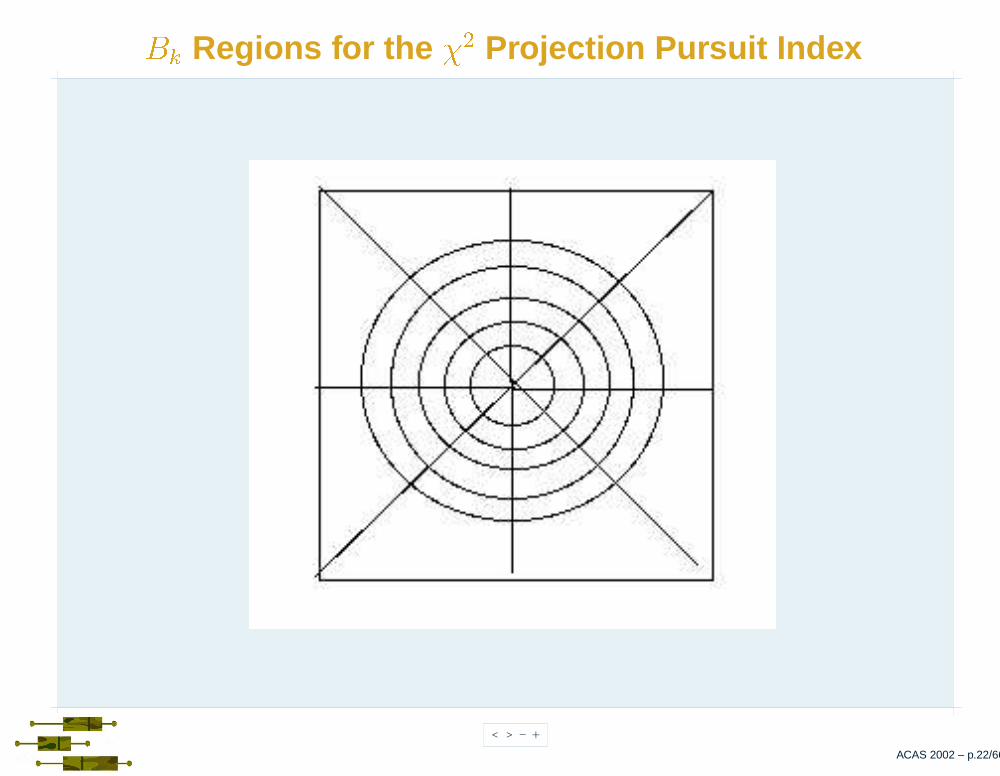
< > - +
��� Regions for the �
�
Projection Pursuit Index
ACAS 2002 – p.22/66
< > - +
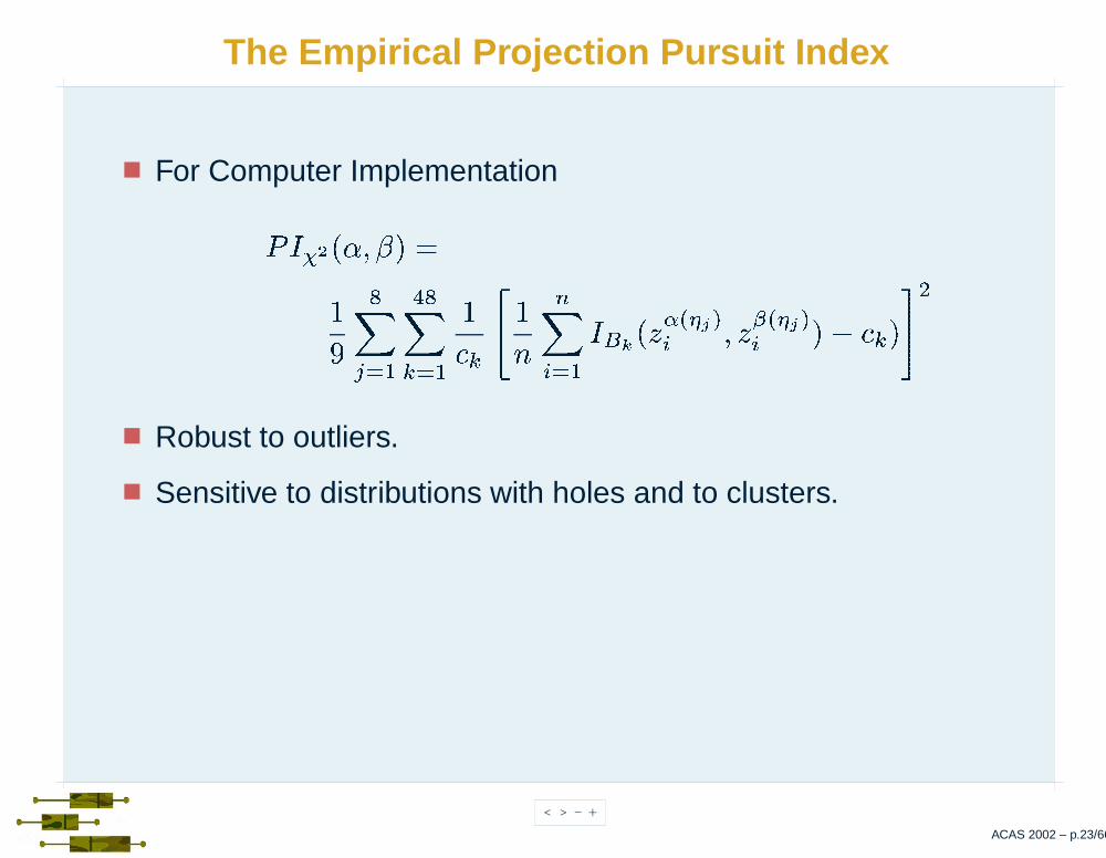
The Empirical Projection Pursuit Index
For Computer Implementation
�� �
� �� � �
��
�
� � �� �
� � ��
��
� ��
�� � �
� � �� � � �� � �� � �� �� � �� � ��
�
Robust to outliers.
Sensitive to distributions with holes and to clusters.
ACAS 2002 – p.23/66

< > - +
Finding the Structure
How do we optimize the projection index over all possibleprojections to
�
?
Method of Posse
� � �� � � � �
� � � � � � �
�� �� � � � � �� � � � �
� � � � � � �� � � � � �
� �� � � � �
� � � � � � �
� �� � � � � � � � �
� � � � � � � � � � �
ACAS 2002 – p.24/66

< > - +
Algorithm - Projection Pursuit Exploratory Data Analysis-I
1. Sphere the data using
�� � � � � � � � � �� � � � � � ��� � � �� �
�
= eigenvectors of
� �
;
�
= diagonal matrix of correspondingeigenvalues,
�� = i-th observation.
2. Generate a random starting plane,
� ���� ��
� � �� � � � � ��� ��
.
3. Calculate the projection index for the starting plane
�� �
� ��� ��
.
4. Generate two candidate planes� � �� ��
and
� � � �
.
5. Evaluate the value of the projection index for these planes,
��� �
� � �� ��
and
��� �
� � � �
.
ACAS 2002 – p.25/66
< > - +
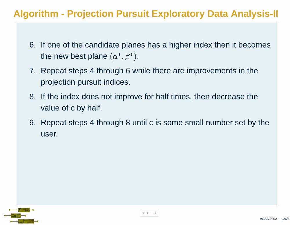
Algorithm - Projection Pursuit Exploratory Data Analysis-II
6. If one of the candidate planes has a higher index then it becomesthe new best plane
� � �� � �
.
7. Repeat steps 4 through 6 while there are improvements in theprojection pursuit indices.
8. If the index does not improve for half times, then decrease thevalue of c by half.
9. Repeat steps 4 through 8 until c is some small number set by theuser.
ACAS 2002 – p.26/66

< > - +
Projection Pursuit Exploratory Data Analysis - Conclusion
Typically an iterative process with structure removed at each stepof the process.
Discriminant analysis needs might lead one to consider alternateprojection pursuit indices.
ACAS 2002 – p.27/66

< > - +
Trees, Graphs and Combining Classifiers
ACAS 2002 – p.28/66

< > - +
Classification Trees
One of the first, and most popular is CART (Classification andRegression Trees).
The idea is to build a tree of simple decision rules.
Each branch of the tree is taken based on a comparison of asingle variable with a value or threshold.
CART implementation issues
How many splits shall we allow at a node?
What properties should be tested at a node?
When should a node be declared a leaf or terminal node?
How shall we prune trees?
If a leaf is impure then how shall we assign the class label?
What shall we do with missing data?
ACAS 2002 – p.29/66

< > - +
CART Iris Analysis
ACAS 2002 – p.30/66

< > - +
CART Details
At each node in the tree, the data is split according to a singlevariable.
The variable and split value are selected in order to best split thedata.
Petal Length<2.45+
Setosa Virginica and Versicolor
The tree is grown until each leaf is pure (single class).
The tree is then pruned to reduce overfitting.
The variables can be continuous or categorical.ACAS 2002 – p.31/66

< > - +
SALAD CART Analysis on Full 13 Bands
This tree uses bands 1,5,7,8,10,12,13.
ACAS 2002 – p.32/66

< > - +
CART Properties
Benefits
CART is an appropriate technique when not much is knownabout the form of an optimal classifier.
CART is an appropriate technique when presented withnon-metric data.
The classifier can often be easily understood as a sequenceof rules, and is thus easily understood by a client.
Like nearest neighbor classifiers, it often produces areasonable classifier for comparison with other techniques.
Missing values are easily incorporated in the classifier.
ACAS 2002 – p.33/66

< > - +
CART Properties
Drawbacks
CART is highly sensitive to the training data set. Smallchanges in the training set can have a marked effect on thenature of the classifier.
Large trees are not really more “understandable” than otherclassifiers.
The decision region is not smooth (an intersection ofrectangles).
ACAS 2002 – p.34/66

< > - +
ID3 and C4.5
The machine learning community has also developed decisiontrees.
ID3 was designed to work on nominal data.
It handles real-valued data via binning.
The algorithm continues until all of the terminal nodes are pure orthere are no more variables to split upon.
C4.5, a follow-on to ID3, is similar to CART, except that differentchoices are made in the design of the tree.
For example, it allows:
Variable numbers of branches from a node.
“Soft” thresholds, to account for observations near thethreshold.
Machine learning is also interested in generating rules, and thereare methods for turning a tree into a set of rules, which can beevaluated by experts, or used in an expert system.
ACAS 2002 – p.35/66

< > - +
Dual Representation of the Linear Classifier
The linear decision function may be rewritten as follow
� � � � � �� � � � � � � �� � � � �� � � � � � � � � �� � � ��Support vector machines are linear classifiers represented in adual fashion.
Data appears within dot products in the decision and trainingfunctions
ACAS 2002 – p.36/66

< > - +
Support Vector Machines (The Cartoon)
We seek a mapping f where we may separate our points via asimple linear classifier
ACAS 2002 – p.37/66

< > - +
Kernels
A function that returns the dot product between the images of thetwo arguments� � � �� � � � � � � � � � � � �
Given a function K it is possible to verify that it is a kernel.
One can use linear classifiers in a feature space by simplyrewriting it in dual representation and replacing dot products withkernels.
ACAS 2002 – p.38/66

< > - +
Kernel Examples
� � �� � � � �� � ��
� � �� � � �� ��� � � � �
� �
Polynomial kernel:
Let � � � � �� �
and � � � ��� �
.
We may write
� �� � � � � � � �� � � �
� � � � � � � � � � � � �� � �
� � � � �� � �
� � � � � � � � �� � �
� � �� � �
� � � � � � � � � � �
ACAS 2002 – p.39/66
< > - +
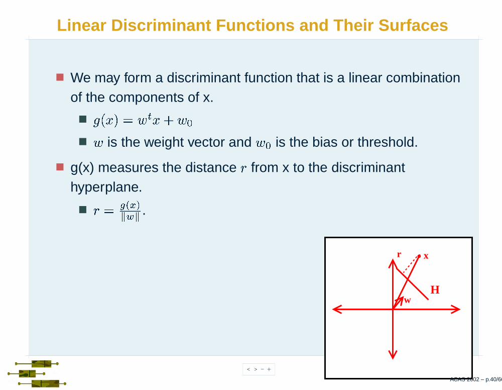
Linear Discriminant Functions and Their Surfaces
We may form a discriminant function that is a linear combinationof the components of x.
�� � � � � � ��
� is the weight vector and �� is the bias or threshold.
g(x) measures the distance � from x to the discriminanthyperplane.
� � � � �� � � .
H
x
w
r
ACAS 2002 – p.40/66

< > - +
Homogeneous Form of the Linear Discriminant Functions
�� � � � � � ��
�� � � �� �
�� � �
�� �� ��
� ��
�� ��
� ��
�������������
�� �
...��
��������������
� ��
�������������
����
...
���
�������������
ACAS 2002 – p.41/66

< > - +
SVM Training Cartoon
R1
R2Margin
Margin
svm
svm
svm
We seek a hyperplane with maximum margin.
The training vectors that define the margins are the supportvectors.
ACAS 2002 – p.42/66

< > - +
SVM Criterion Function - I
Let our training patterns be � � where
� � ��� � � �� �.
Assume the patterns have been subjected to a transformation
�
toproduce � � � � � � � � �
.
Each � � has an associated class � � � � �
.
Our LD in the augmented space is given by
��� � � � .
�� ��� � � ��� � � ��� � � �� �.
ACAS 2002 – p.43/66

< > - +
SVM Criterion Function - II
Recall the distance from our hyperplane to a transformation pointy is given by� � � � �
� � � .
Assuming b a positive margin exists we have
� � � � � �
� � �
� � � � � to ensure uniqueness.
Minimize
� � �
.
ACAS 2002 – p.44/66

< > - +
Solving for the Support Vectors
Choosing
�
Domain knowledge
Polynomials
Gaussians
� � � � � � � � � � � �� � � � � � �� � � � � � �
� � � � �� � � �� � �
����
� � � �� �� �� � � � � .
Subject to
�� � � �� � � � � � � � �� � � ��� � � �� �.
ACAS 2002 – p.45/66

< > - +
A Trivial Example SVM: X-OR
��� � � � � � � � � � � � � �� � � ����
� � � ��
� � � �
� � � � � � � �� �
We seek to maximize�� � � � � � �
����
� � � �� �� �� � � � �
Subject to ��� � � � � � � � � � � � � � � � � � � � � ��� �� � � �
.
ACAS 2002 – p.46/66

< > - +
Two-Dimensional Projection of Six-Dimensional Space
−2 −1.5 −1 −0.5 0 0.5 1 1.5 2−2
−1.5
−1
−0.5
0
0.5
1
1.5
2
g=1
g=−1
2.5x 1x 2
2.5x1
g=0
�� � �� � � � � � � �
.
� � � �
.
Hyperplanes through the support vectors
� � � � � � � �
in themapped space correspond to hyperbolas � � � � � �
in the originalspace.
ACAS 2002 – p.47/66

< > - +
Boosting and Bagging
Many classifiers can be improved by taking aggregates ofclassifiers (ensemble classifiers).
The idea is to construct many classifiers, and combine theirresults into some overall classification.
The simplest of these ideas is Bagging (bootstrap aggregation):
Draw a bootstrap sample of size � � � � and construct acomponent classifier on the sample.
The overall classifier is a vote of the component classifiers.
ACAS 2002 – p.48/66

< > - +
Boosting
The idea of boosting is to construct an ensemble of classifiers,each specialized to the points that previous classifiers haddifficulty with.
Construct a classifier and determine the observations that itmakes errors on.
Reweight the observations to give these difficult observationsgreater weight.
Construct a new classifier on these reweighted observations,and repeat.
The final classifier is a weighted average of the individualones.
ACAS 2002 – p.49/66

< > - +
AdaBoost
Initialize
�� � � ,
� � � �� � � � ��
��
�
,
� � �
Do
k=k+1Train classifier
�� using weights
�� .Variation: train on a bootstrap sample according to
�
.�� � weighted error of
�� .
� � � ��� � � � � �
.
�� � �� �� � � � � � �� � � � �
.Normalize
�
.While
� � �� � � .
Return
� � � � sign�� ��
� � �� � �� � �
ACAS 2002 – p.50/66

< > - +
Class Cover
Assume (for now) that we have two classes whose supports donot intersect (so they are perfectly separable).
Assume further that we have no model for the classes (or theirseparating surface).
The class cover problem is to cover one class (
�
) with balls suchthat none of the balls intersect the other class (
�
).
One way to approximate this is to center balls at
�
observationswith radii no larger than the distance from the observation to any
�
observation.
ACAS 2002 – p.51/66

< > - +
Class Cover Example
�
�
��
��
�
��
��
��
����
��
����
����
We want to cover the support of one class, without covering thatof the other.
ACAS 2002 – p.52/66

< > - +
Class Cover Example
�
�
��
��
�
��
��
��
����
��
����
����
�� !
"#
$%&'
()
*+,-
./01
Circles indicate regions “near” blue observations. They aredefined to be the largest circle centered on a blue that does notcover a red.
ACAS 2002 – p.52/66

< > - +
Class Cover Example
�
�
��
��
�
��
��
��
����
��
����
����
�� !
"#
$%&'
()
*+,-
./01
Blue area shows the decision region for the blue class.
ACAS 2002 – p.52/66

< > - +
Class Cover Catch Digraph
Note that we have one ball per observation, which is more thannecessary. We want to reduce the complexity of the cover.
Define a directed graph (digraph) as follows:
The vertices are the observations from�
.
There is an edge from � � to � if the ball at � � covers � .
We cover the class by a digraph defined by the balls that catch
(contain) the vertices.
We abbreviate this CCCD.
ACAS 2002 – p.53/66

< > - +
CCCD Example
�
�
��
�
��
��
�� �
��
����
����
ACAS 2002 – p.54/66

< > - +
Complexity Reduction
A dominating set of a graph is a set of vertices
�
such that everyvertex is either a member of
�
or has an edge to it from a vertex in
�
.
A minimum dominating set is one which has smallest cardinality.
Denote the cardinality of a minimum dominating set by �.
Note that if we take a minimum dominating set of the CCCD, westill cover all the training observations, thus producing a reducedcover.
ACAS 2002 – p.55/66

< > - +
A Dominating Set
�
�
��
��
�
�
�
�
�
��
����
��
����
����
Note that in this case we obtain a large reduction in complexity and a
“better” class cover.
ACAS 2002 – p.56/66

< > - +
Choosing the Dominating Set
Selecting a minimum dominating set is hard.
A greedy algorithm works well to select a (nearly) minimumdominating set.
The algorithm is fast (given that the interpoint distance matrix hasalready been calculated).
A fast algorithm has been developed which allows the selection ofa small dominating set with large data sizes.
ACAS 2002 – p.57/66

< > - +
The Greedy Algorithm
Select the ball that covers the most
�
points.
While there are still points that are uncovered:
Select the ball that covers the most points not yet covered.
Return the balls selected.
Notes
We do not restrict our selection of balls to those whosecenters are not already covered.
Ties are broken arbitrarily (we can break them in favor of ballswith a higher statistical depth (local density) if we choose).
ACAS 2002 – p.58/66

< > - +
CCCD Classification
The dominating set for the CCCD provides a set of centers andradii.
Compute these for each class.
Compute the minimum scaled distance between a newobservation � and the centers (
� � �� �� � �� ).
The class of the minimum is the class assigned the newobservation.
The CCCD is like a reduced nearest neighbor classifier with avariable metric.
ACAS 2002 – p.59/66

< > - +
CCCD Extensions
One can relax the constraint that the reduced set be a dominatingset by allowing a small number of observations to not be covered.This can simply be done by stopping the greedy algorithm early.
Similarly, one can relax the purity constraint, and allow a smallnumber of other-class observations to be covered. Variousalgorithms are possible, such as only covering a
�
observation ifdoing so covers “enough” new
�
observations.
ACAS 2002 – p.60/66

< > - +
Putting It All Together
We now give an example of a tool that puts all the steps describedtogether.
The tool was designed to operate on images and allow the user toconstruct classifiers to find certain types of objects within images.
This was a “low level” image processing application.
ACAS 2002 – p.61/66

< > - +
Advanced Distributed Region of Interest Tool (ADROIT)
FeatureExtraction
DimensionalityReduction
DiscriminantRegion
Construction
ProbabilityDensity
Estimation
ACAS 2002 – p.62/66
< > - +
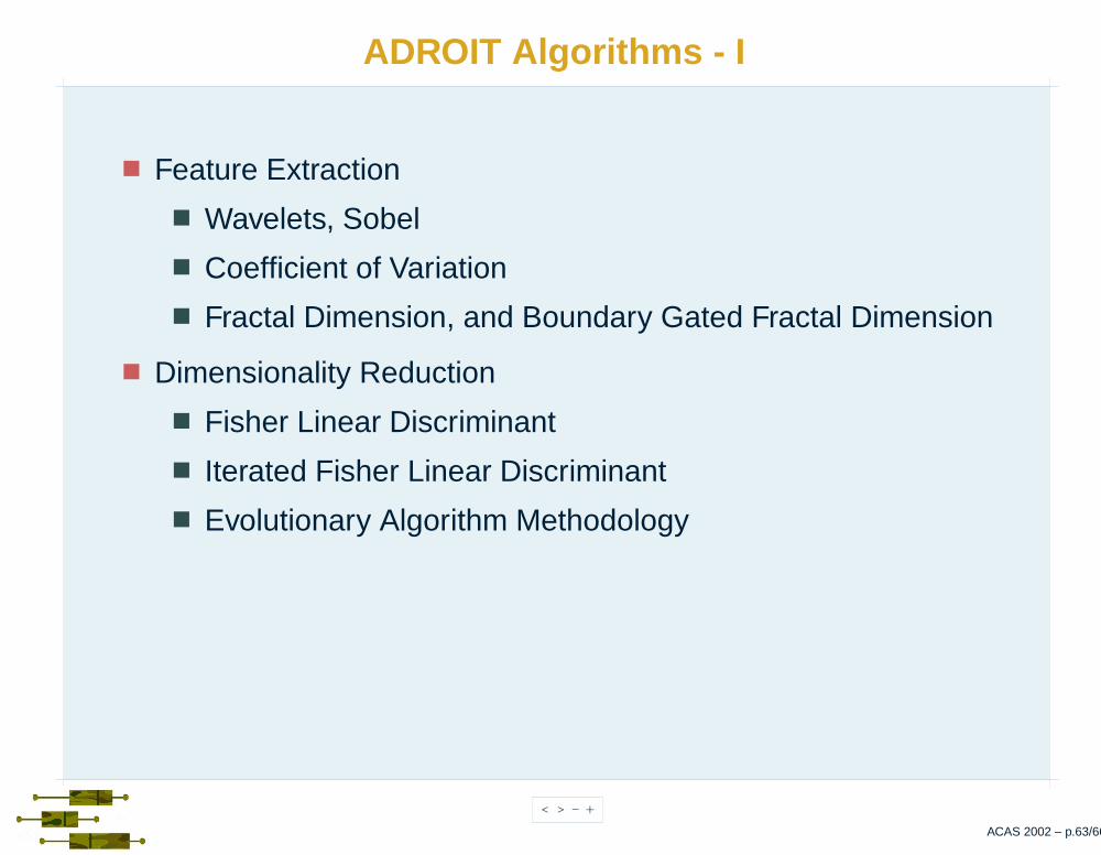
ADROIT Algorithms - I
Feature Extraction
Wavelets, Sobel
Coefficient of Variation
Fractal Dimension, and Boundary Gated Fractal Dimension
Dimensionality Reduction
Fisher Linear Discriminant
Iterated Fisher Linear Discriminant
Evolutionary Algorithm Methodology
ACAS 2002 – p.63/66

< > - +
ADROIT Algorithms - II
Probability Density Estimation
Finite Mixture
Adaptive Mixtures
Classifier Construction
Likelihood Ratio (Bayes Rule)
ACAS 2002 – p.64/66

< > - +
ADROIT Analysis
ACAS 2002 – p.65/66

< > - +
ADROIT Multiclass
ACAS 2002 – p.66/66