Embed Size (px)
Citation preview
The Decline of Competition and Change in Congressional Elections
James E. Campbell and Steve J. JurekDepartment of Political Science
University at Buffalo, SUNYBuffalo, New York 14260
e-mail: [email protected]
in Congress Responds to the Twentieth Century,edited by Sunil Ahuja and Robert Dewhirst,
(Columbus, OH: Ohio State University Press, 2003), pp. 43-72. In the Parliaments and Legislatures Series,
Samuel C. Patterson, General Advisory Editor.

The Decline of Competition and Change in Congressional Elections
Congressional elections changed in many ways over the course of the twentieth century.
At the beginning of the century, the 90 U.S. Senators representing the then 45 states were elected
by their respective state legislatures.1 There were only 357 seats in the U.S. House.2 A number of
these seats in the early decades were elected in multi-member elections, rather than in the now
universally used single member district system. In most years, multi-member districts numbered
fewer than a dozen, but there were 27 such seats in 1912 and the number swelled to 54 in 1932.3
Multi-member or at-large seats existed as late as 1968. Although relatively few third-party
congressional candidates were elected in any election in the century, third party candidates were
present on many ballots throughout the early decades. Cross-endorsements of the same candidate
by several parties (including the major parties) were also common in several states (but
particularly California) in the first part of the century. The size of districts and their turnout also
changed over the years. Turnout in a typical district in the first decade of the century was about
40,000 voters. In the 1990s, despite embarrassingly low turnout rates, the typical district turnout
exceeded 200,000 voters. The geographic distribution of House seats also changed dramatically.
In the century’s opening decade, Florida and California had three and eight seats respectively. By
the century’s closing decade, Florida had 23 seats and California had 52.
There were also enormous changes in how congressional campaigns were conducted.
Much of the change reflected the century’s revolution in communication technology. In the early
1900s, congressional candidates were essentially limited to reaching prospective constituents
directly through stump speeches or indirectly through party workers and local newspaper stories.
The advent of radio, television, mass-mailing technologies, and the Internet, along with scientific
polling and the tremendous increases in campaign spending dramatically altered how
congressional candidates campaigned.
Despite these many changes in congressional elections and campaigning, some
characteristics of congressional elections can be compared across the century. Perhaps the two
most important of these are competition and interelection seat change (the change in the number
of seats for a party as a consequence of an election).
Without competition, elections are meaningless exercises. Competition, the real option
for voters to redirect their representation, is what makes elections important instruments of
representative government. Since the major parties structured American electoral and legislative
politics throughout the twentieth century, the focus of this study is the competition between the
Democrats and the Republicans. By the same token, if voters do not provide some direction to
government through elections, producing meaningful aggregate electoral changes, then even
competitive elections are poor instruments of popular control of the government.
The evaluation of congressional elections over the twentieth century raises several
important questions. How competitive have congressional elections been? How did the extent of
competition between Democratic and Republican candidates change? What affected changes in
the parties’ congressional election fortunes? And how and why have both competition and the
factors affecting interelection seat change evolved over the century?
Before evaluating the extent and change in competition in the twentieth century, we
should note that while competition is to be valued for fueling the electoral incentive for
responsiveness in elected representatives and demonstrating the efficacy of the ballot for
controlling these representatives, competition in extreme doses may not serve the interests of
representative government. Elections that are so competitive that majorities are constantly
turning out representatives at the district level and turning over control of chambers at the

national level may not provide an adequate level of stability. However, the possibility of such
change is important and some regular occurrence of electoral change is necessary to demonstrate
that this possibility is real. Moreover, entrenched majorities may become unresponsive and
permanent minorities may become frustrated with the system. Just how much change or how
close elections must be to provide this beneficial effect without introducing unnecessary
instability is a normative question to keep in mind, but is beyond the scope of answering here.
Our examination of competition and seat change for the parties is organized in three parts.
In the first part, we examine several measures of competition at both the national and constituency
levels for both House and Senate elections. The principal focus is to determine whether there has
been a discernable trend in the competitiveness of congressional elections. The evidence indicates
that there has been a decline in competition, particularly in House elections.4 The second part of
the analysis examines seat change in House and Senate elections. The evidence indicates that
interelection seat change in both the House and Senate have been strongly shaped by presidential
politics. A party’s congressional fortunes in an on-year election are tied to the strength of its
presidential candidate. In midterm elections, the congressional party feels the repercussions of the
previous presidential election in which they stood for election. If congressional candidates were
helped by the top of the ticket in the prior presidential election, they suffer from losing this help in
the midterm. On the other hand, if congressional candidates were hampered by running with a
weak presidential candidate, they tend to run more strongly when they shed this disadvantage in
the midterm. While this presidential pulse of congressional elections continues to provide
important structure to change in congressional politics, there is also evidence that it is weaker than
it once was.5 The third part of the analysis explores one common reason for both the decline in
competition and the weakening of the presidential pulse. As Alan Abramowitz argued in his study

of House elections in the 1970s and 1980s, the huge increases in campaign spending combined
with the great disparity in spending between the candidates have allowed incumbents to secure
their reelections with large margins and provided insulation from the political tides associated
with presidential politics.6
Competition in Congressional Elections
Competition in congressional elections can be evaluated at two levels: the national and
constituency level. Each is important. Competition in national politics– the balance of power
between the parties in the House and in the Senate–has important implications for the course of
national policy. Greater competition nationally makes party government less feasible and may
increase pressures for bipartisanship to sustain governing coalitions. With multiple built-in
roadblocks to governing by a small majority (e.g., veto override requirements, bicameralism,
Senate cloture requirements), narrow party majorities are forced to compromise and to reach
across the aisle for bipartisan cooperation in order to pass legislation. Competition at the district
level (for House races) or at the state level (for Senate races) has direct consequences for voters. It
is at the district or state constituency level that voters in competitive elections may shift party
control and help redirect the course of national politics. How did competition between Democrats
and Republicans at these two levels change throughout the century?
To evaluate the extent and trends in both national and district competition, we examined
several measures of competition. At the national level, two indicators of competition (one static
and one dynamic) were examined. The first indicator was the narrowness of the seat majority.
Elections are more competitive nationally in inverse proportion to the size of a chamber’s
majority. The second indicator is the frequency of alternation in which party holds a chamber’s
majority. A narrow but permanent majority is less indicative of competition than a narrow
majority that shifts control between the parties on a regular basis. The fluidity of control is as
much a consideration in evaluating competition as the size of the majority at any one time. The
first of these indicators is static in that it considers conditions in isolated elections. The second is
dynamic in that it considers conditions of change between elections. The data for these measures
are from Ornstein, Mann, and Malbin’s Vital Statistics on Congress, 1997-1998.7
Five indicators of constituency competition (three static and two dynamic) are examined.
The first is the percentage of all districts or states in which seats are uncontested by one of the
major parties.8 Competition, at least in a minimal sense, is present to the extent that fewer seats
are left uncontested by one of the major parties. The second indicator is the percentage of seats
won by a margin of 55 to 45 percent of the two-party vote or closer. A spread between the
winning and losing major party candidates of ten percent of the vote or less is the conventional
standard of a marginal race. The third indicator is the median winning two-party vote percentage.9
Like marginality, this competition measure examines the apparent ease with which candidates are
elected. More marginal races and lower median winning vote percentages indicate more
competitive politics.
The fourth indicator of constituency competitiveness is the variability in the district or
state vote from one election to the next. This volatility of the local vote is measured as the median
district or state’s percentage point change in the two-party vote from one election to the next. The
real potential for a larger vote change from one election to the next means that more seats cannot
be taken for granted just because they had been won by what appeared to be a comfortable margin
in the previous election. If a district or state had been won with a 60 to 40 vote split in one
election, it may be secure if ten percentage point vote shifts are unusual, but may still be regarded
as competitive if vote swings of this magnitude are common.
The fifth indicator of constituency competition is the percentage of seats in which one
party took the seat from the opposing party that had held the seat prior to the election. In a sense,
this is the ultimate measure of competition. How likely was it that one party was able to
successfully compete to win a seat away from the party previously holding the seat? The
congressional district vote return data used to compute these competition measures were obtained
from Gary King, Congressional Quarterly’s Guide to U.S. Elections, various editions of CQ’s
Politics in America, and Edward Cox’s The Representative Vote in the Twentieth Century.10
National Competition
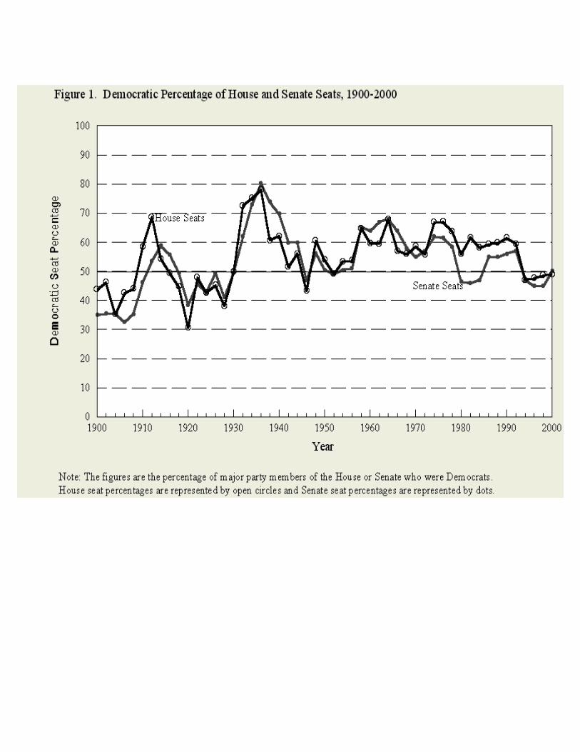
The extent and trend of competition at the national level can be discerned from the plot of
the percentage of House and Senate seats in Figure 1. The most noticeable aspect of this plot is
how closely the parties’ fortunes in House and Senate elections correspond to each other. Since
the popular election of Senators in 1914, the percentage of seats held by Democrats in the House
has been strongly correlated ( r =.81) with their percentage of seats in the Senate.
/Figure 1 about here/
In terms of competition, the closeness of the seat division to the 50 percent line and the
crossing of that line in Figure 1, congressional elections viewed from the national level have been
only modestly competitive in both the House and the Senate. The median election resulted in one
party having 57.5 percent of House seats and 56.6 percent of Senate seats. Congressional elections
have not typically produced near-even divisions, nor have they typically produced extraordinarily
large majorities. As to the turnover of majorities, elections produced new party majorities in only
eight of the 51 congressional elections to the House (16 percent) and in only nine of the 44
popular vote elections of the Senate (21 percent since 1914). At the national level then,
congressional elections have typically produced moderately sized, continuing majorities. This is

what one might expect from a party system that for approximately the first three decades of the
century was decidedly Republican in its bent, for the next 50 years clearly favored the Democrats,
and in the last two decades was quite balanced in its partisanship.
There was no discernable long-term trend in national competition over the century in
either the House or the Senate. The century began with Republican majorities, broken by several
years of Democratic control around the Wilson era, and followed by Democratic New Deal
majorities, broken at several points by Republican post-WWII insurgencies. From the mid-1950s
to 1980, Democrats continuously controlled both chambers with substantial majorities. However
in the closing decades of the century, and particularly in the 1990s, competition for control of both
the House and the Senate were especially keen. However, competition at the national level does
not necessarily reflect competition at the district or state level, where elections are decided.
Competition in the Constituencies
How competitive were typical House and Senate elections in the twentieth century? Table
1 presents the median values from 1920 to 2000 of the five competitiveness indicators for both
House and Senate elections. Elections prior to 1920 were excluded for comparability reasons
because they occurred before the popular election of Senators or before the electoral change
measures could be calculated for Senate elections (the change measures require a prior election).
Like the national level analysis, the constituency measures suggest only a middling level of
competitiveness. In terms of comparing House and Senate elections, Senate elections have
typically been more competitive than House elections. House seats are more than twice as likely
as Senate seats to be uncontested. Whereas fewer than one-fifth of House seats in a typical year
could be characterized as marginal, nearly a third of Senate seats were this closely contested.
While the typical Senate election was decided by a difference of approximately 59 to 41 percent
of the vote, the typical winning margin in House races was nearly 65 to 35 percent. Although there
was little difference between House and Senate elections in the typical amount of vote swing from
one election to the next, because of the greater proportion of closely decided Senate contests, the
typical election shifted party control of nearly a quarter of Senate seats, while elections normally
changed party representation in fewer than one in 10 House seats. As a more valued prize that is
less frequently up for election, Senate seats attracted greater competition than House seats. The
fact that House members constitute an experienced pool of would-be Senate candidates also has
contributed to making Senate elections more closely fought.11
/Table 1 here/
How did the competitiveness of congressional elections change over the century?
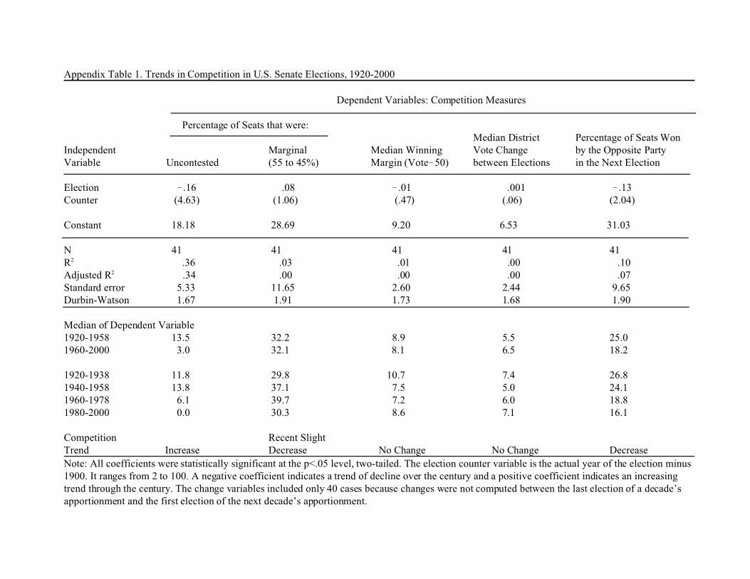
By most indications, competition in Senate elections did not change greatly. There was no
appreciable change in the proportion of Senate seats that were marginal (about a third normally),
or in the median size of winning vote margins, or in the volatility of the vote from one year to the
next.12 Moreover, in terms of nominal competition, far fewer Senate seats went uncontested in
later decades (a decline from a median of 13.5 percent in the 1920-58 period to three percent
since). However, there was a decline in competitiveness in terms of the partisan turnover of seats.
Typically a quarter of all seats were won by a candidate of a different party in Senate elections
from 1920 to 1958 and this declined to about 18 percent of Senate contests in elections in recent
years (see Appendix Table 1).
While competition in Senate elections may have declined slightly, competition in House
elections declined quite a bit over the century. Table 2 presents the trend regressions for each
competition measure along with median values of the indicators over different periods in the
century. The independent variable in these regressions is simply a counter variable reflecting the
year (the last two digits) of the election year. A positive coefficient associated with the counter
reflects a general increase in the measure over the years, while a negative coefficient indicates a
downward trend. In addition to the regressions, to provide a more tangible view of the trends, the
table presents the median values of each of the five competition measures for the first and second
halves of the century and for each quarter of the century. Since an increase in some measures
(uncontested seats and the median winning vote) indicates a decrease in competition, trends are
interpreted in terms of their competition implication in the bottom row of the table.
/Table 2 here/
As the table indicates, while the number of uncontested seats declined a bit and the size of
vote swings increased a bit (both ostensibly signs of increased competition), there was a
substantial decline in the percentage of seats won by narrow margins. Whereas more than 100
seats (in a House of 435) were marginal in the typical election from 1900 to 1948, about 66 fit this
description in the typical post-1976 election. These were, in the immortal words of David
Mayhew, “the vanishing marginals.”13 And this all occurred at the same time that the Democratic
party’s domination of the one-party South was coming to an end–a development that should have
increased the number of competitive districts.
This diminished level of competition was also apparent in a rise in winning vote margins.
Winning candidates won by significantly larger margins (particularly since 1976) and this more
than offset the increased vote swing between election years.14 Although the typical interelection
vote swing increased by about one and a half percentage points in the last quarter of the century
(from about 4.9 to 6.5 percent), the typical winning vote margin rose by nearly four percentage
points.15 The increased apparent volatility of congressional races may have reflected in part the
increase in winning margins. Larger margins are simply more difficult to sustain, causing greater

vote swings from election to election.
As a consequence of the increase in winning vote margins outstripping the increase in
vote change between elections, the likelihood that a district would switch in an election from a
representative of one party to the other party declined substantially. The decline was especially
great in the final quarter of the century.16 Over the first half of the century, nearly 13 percent of
seats were won by a candidate of a party other than the one already holding the seat. In the last
quarter of the century, this rate of party turnover (5.3 percent) was less than half of what it had
been. In short, despite slightly greater interelection vote swings and slightly fewer uncontested
seats, competition in House elections declined significantly over the twentieth century and
particularly in the last quarter of the century. Beneath the competition at the national level at the
century’s close were many districts that were either safely in the Republican column or safely in
the Democratic column. The outcomes of elections in these districts were virtually foregone
conclusions.
Seat Change
As suggested by Figure 1, the net shift of seats for a political party in an election varied a
good deal. Some elections left the status quo intact while others produced rather dramatic changes
in the balance of power between the parties. The 1932 election at the onset of the New Deal
realignment, for instance, shifted nearly one hundred House seats from the Republicans to the
Democrats. Over the century, the typical election shifted about 22 House seats and 5 Senate seats
(median) from one party to the other.
What accounts for the variation in seat change from one election to the next? While many
of the changes are undoubtedly local in nature, different candidates running or retiring and
different issues emerging or receding from local prominence, many of the changes reflect national
political conditions. Interelection seat change in the House for the Democrats over the century can
be largely explained as a function of four variables.17 The first of these is the Democratic
presidential vote margin (the two-party presidential vote for the Democratic candidate minus 50
percent). Its effect on a party’s congressional fortunes is thought to be positive in on-year
elections when presidential coattails help candidates lower on the ticket. This effect provides
important additional congressional support for whichever party wins the presidency. In midterm
elections, however, the hypothesized effect of the previous presidential vote margin in the district
is negative since congressional candidates who had been helped are now stranded without that
support from the top of the ticket. The loss should be commensurate with the magnitude of the
previous support. This dynamic is the impact of the presidential pulse of congressional elections
observed in the theory of surge and decline.18
In addition to the presidential pulse variable, the equation includes the number of seats
won by the party in the previous election. This reflects the fact that it is more difficult to gain
seats if you already hold a large number and, conversely, that it is easier to register gains when a
party has a relatively small number to defend.19 The final two variables reflect the two partisan
realignments of the century, the pro-Democratic New Deal realignment of the 1930s and the pro-
Republican realignment that deepened into congressional politics in the 1990s. The long-term
partisan shifts resulting from these realignments are captured by two dichotomous variables, one
for the 1932 and 1934 elections and the second for the 1992 and 1994 elections. The first should
have a positive coefficient, indicating the shift to Democrats beyond the surge and decline of
short-term forces reflected by the presidential vote margin, and the second should indicate by a
negative coefficient the losses sustained by Democrats as a consequence of the Republican
realignment in the last decades of the century.20
As Table 3 indicates, about three-quarters of net seat shifts for the parties in the U.S. House
over the twentieth century can be explained by the surge and decline of the parties’ presidential
fortunes, each parties’ base or share of seats going into the election, and the two realignments that
took place.21 The estimated effect of each variable is statistically significant and in the expected
direction. Democrats fared better in on-years when their presidential candidate ran a strong race, in
midterms after the Republican presidential candidate had run strongly, when they had fewer seats
to begin with, and as the result of the New Deal realignment. Every percentage point of the
Democratic presidential vote added about three seats to the Democratic column in the House,
though the midterm election reversed these gains by a commensurate amount.22 For every four
seats a party held going into the election, its expected gains were reduced by one seat, reflecting the
fact that a party cannot gain what it already holds. Finally, the New Deal realignment shifted about
63 seats to the Democrats and the Republican realignment of the 1900s shifted about 24 seats to
the Republicans.
/Table 3 here/
The analysis divides the century of elections in half in the last two columns of Table 3. The
seat change equation is estimated first for the 26 elections from 1900 to 1950 and then for the 25
elections from 1952 to 2000. Since the two realignments took place in the different halves of the
century, each realignment variable is only included in the applicable period. In both halves of the
century the equation accounts for nearly three-quarters of the variance in seat change. There are,
however, some important differences. Most notably, the impact of surge and decline in elections in
the second half of the century was only about 80 percent of what it was (3.25 vs. 2.6). Presidential
coattails and the midterm repercussions from them appear to have been shortened in the second
half of the century and these presidential effects were even more seriously eroded in recent
decades.23
There is substantial evidence that one reason for this weakening of the presidential pulse to
congressional elections was the staggered nature of the Republican realignment.24 The greatest
change in the post-1960s Republican realignment occurred in southern states. The lack of a serious
local Republican party in these states complicated and delayed the completion of the realignment.
The South had been solidly Democratic since the end of Reconstruction in the 1870s to the point
that there was virtually no serious local Republican party infrastructure even as late as the 1960s.
Conservative southerners were thus able and willing to vote for Republican presidential candidates
in many areas throughout the South long before they could vote for viable Republican
congressional candidates. In many cases, Republicans failed to put forth a congressional candidate
at all, even in districts in which their presidential candidate won by overwhelming margins.25 It
took several decades before Republicans had assembled a cohort of candidates that could mount
serious challenges to Democratic congressional candidates. The lack of viable Republican
congressional candidates meant that Republican presidential coattails (of Nixon in 1968 and 1972,
of Reagan in 1980 and 1984, and Bush in 1988) were often wasted. The time needed to cultivate
local Republican candidates in the south held back the final chapter in the Republican realignment,
the breakthrough in House elections, and temporarily weakened the pulling power of the
presidential contest on congressional elections.
While wasted coattails may have temporarily diminished the presidential pulse to
congressional elections, the decline in competition may also have weakened presidential effects
and generally reduced the number of seats that changed toward either party as the result of an
election. As indicated in Table 3, the typical seat shift produced by an election in the first half of
the century was about 31 seats. The typical election in the second half of the century, however,
produced a net partisan shift of only 12 or 13 seats. The difference was especially great in the last
quarter of the century. In the 38 elections from 1900 to 1974, 33 (or 87 percent) involved seat
swings of at least ten seats from one party to the other. Of the 13 elections since 1974, only five (or
38 percent) resulted in double-digit seat shifts. With far more seats safely in the hands of one party
or the other, there are fewer seats to be swung either way in elections. In effect, the lack of
competition at the constituency level has made change of any sort at the national level much less
likely and much more difficult.
An analysis of seat shifts in the Senate, using the same model but adjusting for the different
length of the Senate term, essentially confirms the House findings.26 There has been a presidential
pulse to Senate elections which was substantially weakened in the second half of the century and
the net partisan changes in Senate seats resulting from elections were much smaller later in the
century. The median Senate seat shift (after adjusting Senate size to a constant 100 seats) in the 21
elections from 1918 to 1958 was about seven seats. In the 21 elections from 1960 to 2000 the
median net shift of seats from one party to the other was only two seats. The only post-1960
elections in which Senate seats were as great as the earlier seven seat median level were 1980 when
Republicans gained 12 seats, 1986 when Democrats regained eight seats, and 1994 when
Republicans picked up 10 seats. But these were clearly the exceptions. Most Senate elections in
recent years have produced net shifts of no more than a couple of seats one way or the other. In
general then, congressional elections over the century were driven less by presidential elections,
involved fewer seat shifts from one party to the other and, relatedly, were significantly less
competitive than they had been. Congressional elections became less competitive and produced
less partisan change over time.
Incumbency and Campaign Financing
The decline in both competition and interelection seat change is in keeping with findings
that incumbency effects were sizeable and had grown in the last several decades of the century.27
Various electoral advantages have been attributed to congressional incumbency and the increase in
impact on the vote in recent decades. Incumbents have many advantages over challengers. These
include greater name recognition and familiarity to voters, the ability to claim credit for both
general conditions and casework and to stake out issue positions popular with constituents, the
enhancement of their images with the voters through a hospitable “homestyle” and an attentive
permanent campaign from their office, their influence over redistricting to maintain friendly
constituency groups, the early use of these advantages to discourage strong opponents from
mounting a challenge, and the various organizational and informational advantages that come from
having already run and won in the constituency.28 While all of these factors undoubtedly help
incumbents, most are perennial advantages of incumbency and cannot explain why competition
and electoral change declined over the century.
One factor that did change over the century and helped incumbents was the financing of
campaigns.29 Spending on congressional campaigns ballooned in the closing decades of the
century. Between the early 1970s and the late 1990s, total spending on congressional elections
increased nearly ten-fold.30 Substantially more money is spent on congressional races than ever
before. Typically one candidate greatly outspends his or her opponent and the candidate with the
larger war chest is almost always the incumbent. In contested House elections between 1992 and
2000, the incumbent outspent the challenger in 94 to 96 percent of the races. As indicated in Table
4, in the typical House election during this period, the incumbent spent at least five times as much
on the campaign as his or her challenger. In the 2000 election, the median incumbent spent nearly
twelve times what his or her opponent spent. House candidates outspending their opponents by
better than two to one almost always won their election. In the 1990s these incumbents won
between 94 and 99 percent of their elections. When one candidate outspends the other by a large
margin, voters effectively witness a one-sided campaign producing an uncompetitive election.
/Table 4 here/
The situation in the Senate, while not as severe as in the House, also heavily favored
incumbents. Of contested Senate elections from 1992 to 1998 with an incumbent in the race, the
incumbent outspent the challenger 89 percent of the time (86 of 97 elections). As Table 4 shows,
while spending ratios varied from year to year, the incumbent on average spent nearly three dollars
($2.70) for every dollar spent by the challenger. Incumbents who outspent their challengers won 94
percent of their elections, compared to a victory rate of only 64 percent among those who were
outspent by the challenger.
The impact of campaign spending is also evident in a more sophisticated constituency level
analysis (district or state) of the congressional vote. The analysis examines the two-party vote for
the Democratic candidate in contested congressional elections in the 1990s using a fairly simple
regression equation. The equation is estimated separately for House elections in four election years
(1994, 1996, 1998, and 2000) and for the pooled Senate elections from 1992 to 2000. Senate
elections are pooled across years so that all seats could be examined in the same equation and
because of the small number of Senate elections in each election year. The equation explains the
congressional vote as a function of five independent variables: campaign spending, incumbency,
the prior congressional vote, the most recent presidential vote, and the quality of the challenger.
The campaign spending advantage variable is the difference between campaign expenditures of the
Democratic and Republican candidates as a percentage of spending by both candidates. The
variable ranges from a value of one, when the Democratic candidate spends all of the money in the
race, to negative one, when the Republican does all of the spending. A value of zero indicates that
both candidates spent an equal amount on the campaign. This index has a number of virtues
including taking into account the interactive and nonlinear aspects of campaign spending effects.31
The incumbency advantage variable is scored +1 when a Democratic incumbent is seeking
reelection, -1 when a Republican incumbent is running, and 0 when the seat is open. The prior
Democratic congressional vote refers to the vote in the constituency in the last election for that
seat. The Democratic two-party presidential vote in the constituency is used here as a measure of
constituency partisanship. Finally, the quality of the challenger is assessed by whether the
challenger had previously been successful in attaining elective office. The challenger quality
variable is score +1 when a Democratic challenger had previously held elective office and -1 when
the he or she had not. The coding is reversed for Republican challengers (-1 for experienced
Republican challengers and +1 for inexperienced Republicans (a Democratic advantage)). When
both or neither candidate in an open seat contest have held elective office the variable is scored 0.
Since all Senate candidates are highly visible to voters, the challenger variable was not included in
the Senate regression.
The regression results are reported in Table 5. As the table indicates, the five variable
model does an exceedingly good job of explaining the congressional vote. The equation explains
anywhere from 90 to 95 percent of variance in the House vote (the adjusted R2s). Although Senate
elections are higher profile contests and are more heavily influenced by local factors such as the
personal and policy strengths and weaknesses of the candidates and their campaigns, the Senate
equation accounts for more than three-quarters of the variance in the Senate vote. Combining the
campaign spending values for incumbents with the estimated coefficients indicates that the typical
advantage of both House and Senate incumbents (median campaign spending advantage values of
.46 for Senate incumbents and between .66 and .84 for House incumbents) adds anywhere from
seven to eleven percentage points to their vote shares compared to the expected vote if incumbents
and challengers spent equal amounts. By these calculations, the campaign spending advantage of
incumbents dwarfs the estimated two to three point advantages from all other incumbency
advantages. In short, the much vaunted incumbency advantage would appear to be substantially a
campaign spending advantage.32
/Table 5 here/
The paramount importance of the campaign spending advantage may also be seen by an
inspection of the regressions’ standardized coefficients (in parentheses in Table 5). The
standardized coefficients indicate the relative importance of the variables in explaining variation in
the vote. In each of the four regressions, covering more than a thousand House races and more than
one hundred Senate contests, the campaign spending advantage was far and away the most
important variable in determining the congressional vote.33 It was more important than
incumbency, the presidential vote, and even the prior congressional vote. The simple correlations
between campaign spending and the vote (in the bottom row) also show just how closely campaign
spending is now related to the congressional vote. The correlation of spending and the vote could
hardly be any stronger.
While our focus has been on the campaign spending advantage enjoyed by most
incumbents, the effects of campaign spending on boosting the vote out of the competitive range are
not restricted to incumbents exclusively.34 While open seat races are more often competitive, some
candidates in these races are able to greatly outspend their opponents to the point that the election
is no longer seriously competitive. In the typical open seat contested House race in 1998, for
instance, the winning candidate outspent the opposition by 2.5 to 1. When winning candidates in
these open seat races outspent their opposition by more than 2.5 to 1, the race was seldom (11
percent) decided in the marginal vote range. When spending was more evenly balanced than this,
the outcome was quite often (72 percent) decided as a marginal contest.
Unfortunately campaign spending data before the 1970s do not exist, and so we cannot
directly test the proposition that campaign financing has led to diminished competition, reduced
interelection seat change, and a weakening of the presidential surge and decline in congressional
elections. However, it is nevertheless probably quite safe to say (1.) that more money is now spent
on congressional elections than ever before, (2.) that campaign spending matters a great deal to the
vote, and (3.) that campaign spending is lopsidedly in favor of one of the candidates, normally the
incumbent. Based on these facts, it is difficult to escape the conclusion that the amount of
campaign spending and the disparity in it has reduced competition in congressional elections. With
diminished competition, fewer seats being truly “in play” in an election, the possibilities of
electoral change in tandem with the presidential vote are greatly reduced as well.
Conclusion
As the century closed and the new one began, congressional politics at the national level
looked highly competitive. Republicans held razor-thin majorities in both the House and the
Senate. After the 2000 election, until Vermont’s Senator James Jeffords left the party, Republicans
controlled an evenly divided Senate by virtue of the tie-breaking vote of Republican Vice President
Richard Cheney. In the House of Representatives, Republicans had a mere five seat majority.
However, the competitiveness of the parties at the national level belied a far less competitive
situation at the congressional district and state levels. Congressional elections in many districts and
states had become mere formalities. David Broder, reporting in early September on congressional

campaigns of 2000, observed that “barely four dozen districts”of the total of 435 could be
described as being “seriously in play.”35 The chance that the vast majority of congressional
elections would make any difference had become remote.
Although noncompetitive elections outnumbered competitive elections throughout the
century, competition was far more common in the first part of the century than in the century’s
closing decades. Even when Republicans dominated national politics in the first 30 years of the
century or when Democrats dominated in the following 30 years (and dominated in the South to
the virtual exclusion of Republicans from the end of Reconstruction until the 1980s), competitive
elections had been more common. Both the gross amount of seat change (a seat changing either
way in an election (Table 2)) and the net amount of seat change (net partisan gains or losses (Table
3)) in House elections after 1970 were typically less than half of what they had been in earlier
years. Perhaps because Senate seats have a broader pool of quality candidates and the campaign
spending disparities had not typically been as severe, the decline in competition in Senate elections
was not nearly so great.
The decline in competition was not the only change in congressional elections in the
twentieth century. Congressional elections changed in a number of important respects and several
of these changes appear to be linked. As Alan Abramowitz found in his study of House elections in
the 1970s and 1980s, we found that increased spending on congressional campaigns, especially by
incumbents, had the effect of diminishing competition and providing additional insulation of
congressional elections from national political tides.36 Occasionally, as in the 1994 midterm
breakthrough election for the Republicans, the tides were strong enough to overwhelm the
considerable campaign spending advantage of incumbents. But elections of this sort were the rare
exception. Most congressional elections at the end of the twentieth century produced relatively

small seat shifts toward either party because few seats were competitive enough that candidates of
either party stood a real chance of winning them. A major factor in setting aside so many seats as
either safely in the hands of the Democrats or safely held by Republicans appears to be the relative
financing of the major party candidates. Congressional incumbents hold their seats more safely
than ever because they have the finances to run campaigns that drown out their opposition’s
campaign.
In a sense, the decline of competition and of seat changes in congressional elections have
greatly reduced the importance of elections as instruments for the public to hold those in
government accountable. If the stability in congressional vote had simply reflected stable voter
preferences, one could conclude that elections did not produce change because voters did not want
change. Elections would still be available as instruments of democratic control, if and when voters
chose to use them. However, the analysis in Table 5 indicated that the stability of voter preferences
is a rather distant secondary reason for the lack of change. Incumbent-friendly campaign financing
and incumbency have had much more to do with preserving the status quo. As such, while we
cannot say how much competition is optimal for the system, it is probably safe to say that it is not
healthy for democracy to have a considerable amount of competition bought off through campaign
financing disparities. From the standpoint of representation, it might also be supposed that the
electoral security purchased by their campaign spending advantage has reduced the pressure on
incumbents to please their constituencies.
With party competition so evenly balanced at the national level, it seems likely that
America will have two types of politics across the country for the foreseeable future. In those states
and districts that remain competitive, competition is likely to intensify. Since these areas are now
relatively few and hold the key to control of the House or Senate, the parties and their supporters
will fight no-holds-barred contests to win these seats. Most voters, however, will not experience
this competitive ferocity. Most of the nation suffers from competition anemia as voters sleepwalk
through the campaign to the anointing of the preordained winner. In their political malaise, unless
and until some radical reform of campaign financing is undertaken to rectify the huge imbalances
in campaign resources (reform not seriously contemplated in national politics at this time), voters
can only watch the high priced candidate television ads extolling the supposed virtues of their
incumbents and lament that congressional elections are not what they used to be.

Table 1. Comparison of Competition in House and Senate Elections, 1920-2000
Competition Measure
Percentage of Seats that wereMedian District Percentage of Seats Won
Marginal Median Winning Vote Change by the Opposite Party Elections for Uncontested (55 to 45%) Margin (Vote!50) between Elections in the Next Election
House 17.8 18.8 14.5 5.4 8.8
Senate 8.3 32.1 8.6 6.4 23.1
More Competition Senate Senate Senate No Difference Senate
Note: The entries are median values for each indicator. The series starts with 1920 to maintain comparability between the House and the Senate.Senators were elected by state legislatures until 1914. The vote and outcome change measures could not be calculated until the 1914 class of seatshad been elected for a second term in 1920. The number of elections over which these medians are calculated is 41, except for the vote change andoutcome change indicators for House elections. These changes are not computed across elections in which general reapportionment took place. Themedians for these two variables are based on 33 elections. The median for House elections since 1900 are within one percentage point off each ofthe post-1920 medians and do not alter any of the House-Senate comparisons.
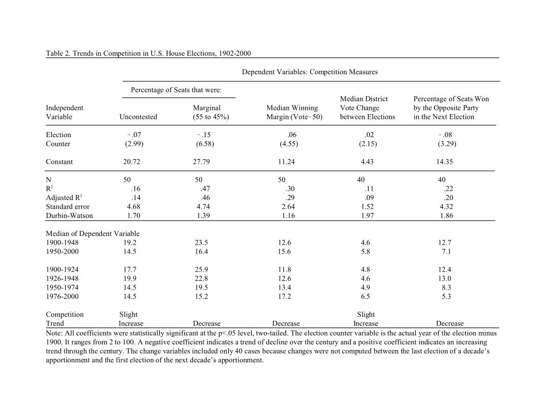
Table 2. Trends in Competition in U.S. House Elections, 1902-2000
Dependent Variables: Competition Measures
Percentage of Seats that were:Median District Percentage of Seats Won
Independent Marginal Median Winning Vote Change by the Opposite Party Variable Uncontested (55 to 45%) Margin (Vote!50) between Elections in the Next Election
Election !.07 !.15 .06 .02 !.08Counter (2.99) (6.58) (4.55) (2.15) (3.29)
Constant 20.72 27.79 11.24 4.43 14.35
N 50 50 50 40 40R2 .16 .47 .30 .11 .22Adjusted R2 .14 .46 .29 .09 .20Standard error 4.68 4.74 2.64 1.52 4.32Durbin-Watson 1.70 1.39 1.16 1.97 1.86
Median of Dependent Variable1900-1948 19.2 23.5 12.6 4.6 12.71950-2000 14.5 16.4 15.6 5.8 7.1
1900-1924 17.7 25.9 11.8 4.8 12.4 1926-1948 19.9 22.8 12.6 4.6 13.0 1950-1974 14.5 19.5 13.4 4.9 8.3 1976-2000 14.5 15.2 17.2 6.5 5.3
Competition Slight SlightTrend Increase Decrease Decrease Increase Decrease
Note: All coefficients were statistically significant at the p<.05 level, two-tailed. The election counter variable is the actual year of the election minus1900. It ranges from 2 to 100. A negative coefficient indicates a trend of decline over the century and a positive coefficient indicates an increasingtrend through the century. The change variables included only 40 cases because changes were not computed between the last election of a decade’sapportionment and the first election of the next decade’s apportionment.
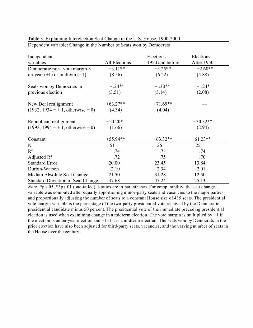
Table 3. Explaining Interelection Seat Change in the U.S. House, 1900-2000Dependent variable: Change in the Number of Seats won by Democrats
Independent Elections Electionsvariables All Elections 1950 and before After 1950
Democratic pres. vote margin × +3.11** +3.25** +2.60**on-year (+1) or midterm (!1) (8.56) (6.22) (5.88) Seats won by Democrats in !.24** ! .30** ! .24*previous election (3.51) (3.14) (2.08)
New Deal realignment +63.27** +71.69** —(1932, 1934 = + 1, otherwise = 0) (4.34) (4.04)
Republican realignment !24.20* — !30.32**(1992, 1994 = + 1, otherwise = 0) (1.66) (2.94)
Constant +55.94** +63.32** +61.23**N 51 26 25R2 .74 .78 .74Adjusted R2 .72 .75 .70Standard Error 20.00 23.45 13.84Durbin-Watson 2.10 2.34 2.01Median Absolute Seat Change 21.50 31.28 12.50Standard Deviation of Seat Change 37.68 47.24 25.13Note: *p#.05, **p#.01 (one-tailed). t-ratios are in parentheses. For comparability, the seat changevariable was computed after equally apportioning minor-party seats and vacancies to the major partiesand proportionally adjusting the number of seats to a constant House size of 435 seats. The presidentialvote margin variable is the percentage of the two-party presidential vote received by the Democraticpresidential candidate minus 50 percent. The presidential vote of the immediate preceding presidentialelection is used when examining change in a midterm election. The vote margin is multiplied by +1 ifthe election is an on-year election and !1 if it is a midterm election. The seats won by Democrats in theprior election have also been adjusted for third-party seats, vacancies, and the varying number of seats inthe House over the century.
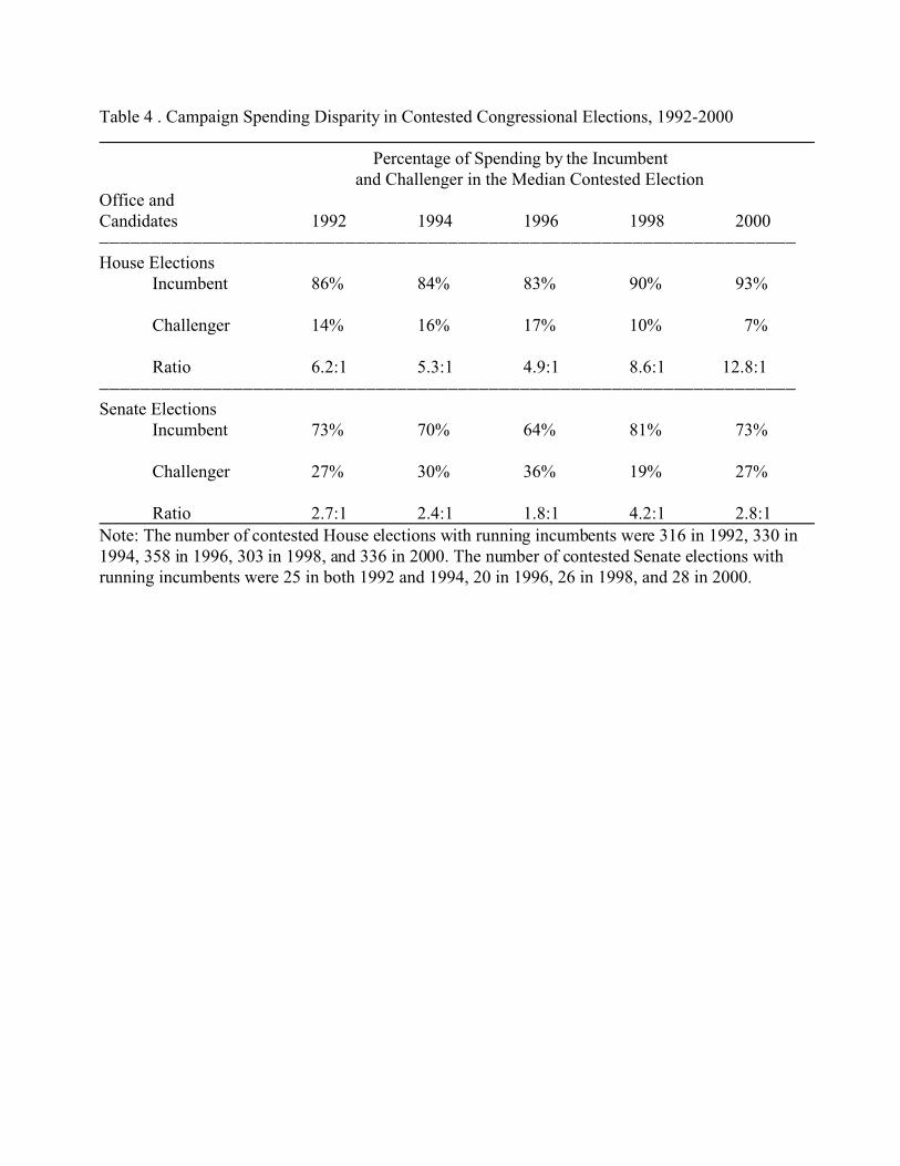
Table 4 . Campaign Spending Disparity in Contested Congressional Elections, 1992-2000
Percentage of Spending by the Incumbent and Challenger in the Median Contested Election
Office andCandidates 1992 1994 1996 1998 2000))))))))))))))))))))))))))))))))))))))))))))))))))))))))))))))))))))
House ElectionsIncumbent 86% 84% 83% 90% 93%
Challenger 14% 16% 17% 10% 7%
Ratio 6.2:1 5.3:1 4.9:1 8.6:1 12.8:1))))))))))))))))))))))))))))))))))))))))))))))))))))))))))))))))))))
Senate ElectionsIncumbent 73% 70% 64% 81% 73%
Challenger 27% 30% 36% 19% 27%
Ratio 2.7:1 2.4:1 1.8:1 4.2:1 2.8:1Note: The number of contested House elections with running incumbents were 316 in 1992, 330 in1994, 358 in 1996, 303 in 1998, and 336 in 2000. The number of contested Senate elections withrunning incumbents were 25 in both 1992 and 1994, 20 in 1996, 26 in 1998, and 28 in 2000.
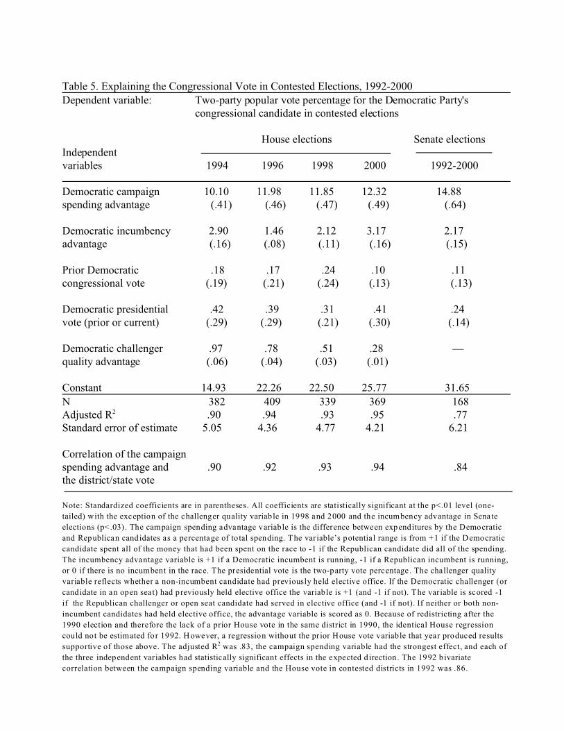
Table 5. Explaining the Congressional Vote in Contested Elections, 1992-2000Dependent variable: Two-party popular vote percentage for the Democratic Party's
congressional candidate in contested elections
House elections Senate electionsIndependent variables 1994 1996 1998 2000 1992-2000 Democratic campaign 10.10 11.98 11.85 12.32 14.88spending advantage (.41) (.46) (.47) (.49) (.64)
Democratic incumbency 2.90 1.46 2.12 3.17 2.17advantage (.16) (.08) (.11) (.16) (.15)
Prior Democratic .18 .17 .24 .10 .11congressional vote (.19) (.21) (.24) (.13) (.13) Democratic presidential .42 .39 .31 .41 .24 vote (prior or current) (.29) (.29) (.21) (.30) (.14)
Democratic challenger .97 .78 .51 .28 — quality advantage (.06) (.04) (.03) (.01)
Constant 14.93 22.26 22.50 25.77 31.65
N 382 409 339 369 168 Adjusted R2 .90 .94 .93 .95 .77Standard error of estimate 5.05 4.36 4.77 4.21 6.21
Correlation of the campaignspending advantage and .90 .92 .93 .94 .84the district/state vote
Note: Standardized coefficients are in parentheses. All coefficients are statistically significant at the p<.01 level (one-
tailed) with the exception of the challenger quality variable in 1998 and 2000 and the incumbency advantage in Senate
elections (p<.03). The campaign spending advantage variable is the difference between expenditures by the Democratic
and Republican cand idates as a percentage of total spending. The variable’s potential range is from +1 if the Democratic
candidate spent all of the money that had been spent on the race to -1 if the Republican candidate did all of the spending.
The incumbency advantage variable is +1 if a Democratic incumbent is running, -1 if a Republican incumbent is running,
or 0 if there is no incumbent in the race. The presidential vote is the two-party vote percentage. The challenger quality
variable reflects whether a non-incumbent candidate had previously held elective office. If the Democratic challenger (or
candidate in an open seat) had previously held elective office the variable is +1 (and -1 if not). The variable is scored -1
if the Republican challenger or open seat candidate had served in elective office (and -1 if not). If neither or both non-
incumbent candidates had held elective office, the advantage variable is scored as 0. Because of redistricting after the
1990 election and therefore the lack of a prior House vote in the same district in 1990, the identical House regression
could not be estimated for 1992. However, a regression without the prior House vote variable that year produced results
supportive of those above. The adjusted R2 was .83, the campaign spending variable had the strongest effect, and each of
the three independent variables had statistically significant effects in the expected d irection. The 1992 b ivariate
correlation between the campaign spending variable and the House vote in contested districts in 1992 was .86.
Appendix Table 1. Trends in Competition in U.S. Senate Elections, 1920-2000
Dependent Variables: Competition Measures
Percentage of Seats that were:Median District Percentage of Seats Won
Independent Marginal Median Winning Vote Change by the Opposite Party Variable Uncontested (55 to 45%) Margin (Vote!50) between Elections in the Next Election
Election !.16 .08 !.01 .001 !.13Counter (4.63) (1.06) (.47) (.06) (2.04)
Constant 18.18 28.69 9.20 6.53 31.03
N 41 41 41 41 41R2 .36 .03 .01 .00 .10Adjusted R2 .34 .00 .00 .00 .07Standard error 5.33 11.65 2.60 2.44 9.65Durbin-Watson 1.67 1.91 1.73 1.68 1.90
Median of Dependent Variable1920-1958 13.5 32.2 8.9 5.5 25.01960-2000 3.0 32.1 8.1 6.5 18.2
1920-1938 11.8 29.8 10.7 7.4 26.8 1940-1958 13.8 37.1 7.5 5.0 24.1 1960-1978 6.1 39.7 7.2 6.0 18.8 1980-2000 0.0 30.3 8.6 7.1 16.1
Competition Recent Slight Trend Increase Decrease No Change No Change Decrease
Note: All coefficients were statistically significant at the p<.05 level, two-tailed. The election counter variable is the actual year of the election minus1900. It ranges from 2 to 100. A negative coefficient indicates a trend of decline over the century and a positive coefficient indicates an increasingtrend through the century. The change variables included only 40 cases because changes were not computed between the last election of a decade’sapportionment and the first election of the next decade’s apportionment.

Appendix Table 2. Explaining Interelection Seat Change in the U.S. Senate, 1918-2000
Dependent variable: Change in the Percentage of Seats held by Democrats
Independent Elections Electionsvariables All Elections 1958 and before After 1958
Democratic pres. vote margin ×on-year (+1) +.31** +.41** + .12or prior vote (t-6) × midterm (!1) (3.29) (2.80) (.86) Percentage of Seats that are up ! .24** ! .23** !.23** that were held by Democrats (4.28) (2.59) (3.06)
New Deal realignment +6.73** + 5.97 —(1932, 1934, 1936 = +1 otherwise = 0) (2.41) (1.68)
Republican realignment ! 4.96* — !4.64*(1992, 1994, 1996 = +1, otherwise = 0) (1.86) (1.88)
Constant +13.06** +12.61** +11.28**
N 42 21 21R2 .62 .72 .42Adjusted R2 .58 .66 .32Standard Error 4.36 4.82 3.86Durbin-Watson 2.16 2.01 1.99
Median Absolute Percentage Seat Change 4 .58 7.29 2.00 Standard Deviation of Percentage Seat Change 6 .70 8.32 4.69Note: *p#.05, **p#.01 (one-tailed). t-ratios are in parentheses. For comparability, the dependent variable is the change as the result of the
election in the percentage of Senate seats held by Democrats. Also for comparability across years, seats held by independents or third-parties
are divided evenly between the major parties. The presidential vote margin variable is the percentage of the two-party presidential vote
received by the Democratic presidential candidate minus 50 percent. The presidential vote of the immediate preceding presidential election is
used when examining change in a midterm election. The vote margin is multiplied by +1 if the election is an on-year election and !1 if it is a
midterm election. The percentage of seats held by Democrats that are up for election are computed from all seats that were up for election in
that year.

1. The 17th Amendment to the U.S. Constitution provided for the popular election of U.S.Senators. The amendment was ratified in 1913 and took effect in the 1914 midterm congressionalelections.
2.The number of seats in the U.S. House of Representatives was increased to 386 seats for the1902 election, 391 for the 1908 election, and finally its present number of 435 for the 1912election.
3.Multi-member districts were generally used in one of three situations: (1.) in relatively smallpopulation states with two seats, (2.) after a reapportionment, but before the state could agree onnew district lines, and (3.) for one or two at-large seats in a state with other districted seats.
4. See, David R. Mayhew, Congress: The Electoral Connection (New Haven: Yale UniversityPress, 1974) and "Congressional Elections: The Case of the Vanishing Marginals," Polity 6(1974) 295-318; Albert D. Cover and David R. Mayhew, "Congressional Dynamics and theDecline of Competitive Elections," in Congress Reconsidered, Second Edition ed. Lawrence C.Dodd and Bruce I. Oppenheimer (Washington, D.C.: Congressional Quarterly Press, 1981), 62-82; and James C. Garand and Donald A. Gross, "Changes in the Vote Margins for CongressionalCandidates: A Specification of Historical Trends," American Political Science Review 78(1984):17-30.
5. See James E. Campbell, "The Presidential Surge and its Midterm Decline in CongressionalElections," The Journal of Politics 53 (1991): 477-87; "The Presidential Pulse of CongressionalElections, 1868-1988." in The Atomistic Congress ed. by Allen D. Hertzke and Ronald M. Peters,Jr., (Armonk, N.Y.: M.E. Sharpe, 1992): 49-72; and The Presidential Pulse of CongressionalElections, Second Edition (Lexington, KY: The University Press of Kentucky, 1997).
6. Alan I. Abramowitz, “Incumbency, Campaign Spending, and the Decline of Competition inU.S. House Elections,” The Journal of Politics 53 (1991): 34-56.
7. Normal J. Ornstein, Thomas E. Mann, and Michael J. Malbin, Vital Statistics on Congress,1997-1998 (Washington, D.C.: American Enterprise Institute, 1998).
8. See, Peverill Squire, "Competition and Uncontested Seats in U.S. House Elections."Legislative Studies Quarterly 14 (1989): 281-95 and J. Mark Wrighton and Peverill Squire,"Uncontested Seats and Electoral Competition for the U.S. House of Representatives OverTime," (paper delivered at the annual meeting of the Midwest Political Science Association,Chicago, April 1995).
9. See Garand and Gross, “Changes in the Vote Margins for Congressional Candidates: ASpecification of Historical Trends,” and James C. Garand, Kenneth Wink, and Bryan Vincent,"Changing Meanings of Electoral Marginality in U.S. House Elections, 1824-1978." PoliticalResearch Quarterly 46 (1993): 27-48 and Gary C. Jacobson "Getting the Details Right: AComment on `Changing Meanings of Electoral Marginality in U.S. House Elections, 1824-1978'," Political Research Quarterly 46 (1993): 49-54.
Notes
10. See Gary King, Elections to the U.S. House of Representatives: 1898-1992, ICPSR StudyNumber 06311 (1994); Congressional Quarterly, Guide to U.S. Elections, 2nd ed. (Washington,D.C.: Congressional Quarterly, 1985); Alan Ehrenhalt, ed. Politics in America (Washington,D.C.: CQ Press,1983, 1985,1987); Phil Duncan, ed. Politics in America (Washington, D.C.: CQPress, 1989, 1991, 1993); Phil Duncan and Christine C. Lawrence, eds. Politics in America(Washington, D.C.: CQ Press, 1995, 1997); Phil Duncan and Brian Nutting, eds. Politics inAmerica (Washington, D.C.: CQ Press, 1999); and Edward Franklin Cox, The RepresentativeVote in the Twentieth Century (Bloomington, IN: The Institute of Public Administration, 1981).The dynamic or across-elections measures of competition are not computed between eachdecade’s reapportionments since changing district boundaries make comparisons inappropriate.While some redistrictings have occurred during a decade (see Cox The Representative Vote in theTwentieth Century, 7) basic district identities have been maintained so that districts can bematched up from one election to the next. Nevertheless, the disruptions of district borders in themiddle of decades may have the effect of inflating vote and outcome change measures. Some ofthis problem may be mitigated, however, by the use of multi-member at-large elections prior toredistricting later in the decade. Multi-member districts are not included in this analysis.
11. John R. Alford and John R. Hibbing in “Electoral Convergence in the U.S. Congress” in Bruce I. Oppenheimer (ed.) Senate Exceptionalism (Columbus, OH: Ohio State University Press,forthcoming) conclude that the Senate and House are converging in their electoral sensitivity orresponsiveness. That is, the two houses are now about equally likely to change as the result of anelection. Their conclusion is based on an analysis of switches in partisan control of eachchamber, tenure and turnover of the membership of each chamber, and the swing ratios (howmany seats are shifted between parties by a change in the popular vote). The current analysis isnot inconsistent with these findings. While individual Senate elections are likely to be morecompetitive than individual House elections, the greater frequency of House elections (becauseof the shorter term) makes up for the difference. Additional, it would seem that while to twochambers are becoming similarly sensitive to electoral forces, the convergence is more the resultof House elections becoming less sensitive than Senate elections becoming more sensitive toelectoral forces. This is suggested by their estimate of a generally declining swing-ratio forHouse elections.
12. Donald Gross and David Breaux in “Historical Trends in U.S. Senate Elections, 1912-1988"American Politics Quarterly, 19 (1991): 284-309 also find a slight decline in competition inSenate elections. However, they note that the decline was much more pronounced in nonsouthernstates. An increase in competition within Southern states largely offset the greater nonsoutherndecline.
13. Mayhew, "Congressional Elections: The Case of the Vanishing Marginals."
14. James Garand and Donald Gross in examining House elections up to 1980 found evidence ofa long-term trend of declining competition (as measured by the average winning vote margin)since 1894, but they found no further decrease in elections from 1966 to 1980. See Garand andGross "Changes in the Vote Margins for Congressional Candidates: A Specification of HistoricalTrends," and Donald A. Gross and James C. Garand, “The Vanishing Marginals, 1824-1980,”The Journal of Politics 46 (1984): 224-237.. The regression in Table 2 concurs with Garand andGross’ finding of a general increase in the size of winning vote margins through the century.

However, inspection of the median vote margins by the century’s quarters, as well as a dummyvariable analysis of the margin levels in each quarter, indicates that the increase in winningmargins was greatest in elections since 1975. The dummy variable analysis, assigning a separatedichotomous variable to elections in each quarter of the century, indicated positive but notstatistically significant increases for the second and third quarters of the century (.6 and 1.1percentage point increases over the first quarter) and a statistically significant and positiveincrease (4.6 percentage points) in the final quarter century. The analysis indicates that medianwinning vote margins in fourth quarter were significantly higher than they were elections in thethird quarter.
15. For a time it was thought that the increased volatility in the congressional vote entirely offsetthe higher winning vote margins. If so, there would have been no decline in competition, acandidate who in the volatile vote years won with a margin of 60 percent might have no reason tofeel any safer for reelection than a candidate who in the nonvolatile vote years won with a marginof 55 percent. Gary Jacobson claimed that the marginals never truly vanished since winning by alarge margin did not mean what it once did. See Gary C. Jacobson, “The Marginals NeverVanished: Incumbency and Competition in Elections to the U.S. House of Representatives, 1952-82," American Journal of Political Science 31 (1987): 126-41. Garand, Wink, and Vincent alsoexamined vote volatility (interelection vote swing) and the chances of reelection or defeat andfound that the actual vulnerability of an incumbent to defeat in the next election was a function ofboth the volatility of the vote and the magnitude of the prior victory. See Garand, Wink, andVincent, "Changing Meanings of Electoral Marginality in U.S. House Elections, 1824-1978." While this study concurred with Jacobson’s principal theoretical point, Jacobson claimed thattheir estimates of mean vote margins and mean vote swings were exaggerated by the inclusion ofuncontested districts. See Jacobson, "Getting the Details Right: A Comment on `ChangingMeanings of Electoral Marginality in U.S. House Elections, 1824-1978." Including uncontesteddistricts makes the electorate look less evenly divided and more volatile than it really is sincevoters have no control over whether their districts will be contested or not. On the other hand,excluding these districts and only examining contested districts raises other problems ofcomparability across election years and excluding nominally uncontested districts whileincluding those with merely token candidates. By examining the median, rather than mean levelsof vote margins and vote swings, this analysis avoids both the pitfalls. These measures are notdistorted by the skewing effect of uncontested districts and also considers all districts rather thansome varying subset of districts.
16. A dummy variable regression, assigning a separate dichotomous variable to election in eachquarter of the century, indicated that seat turnover from one party to another was significantlylower in the final quarter of the century than it had been in prior elections, though the percentageof seats subsequently won by the opposing party in the next election declined throughout thecentury. Of particular note, when the third quarter dummy is omitted and serves as a baseline, thefourth quarter dummy coefficient is statistically significant and indicates a decline of 3.3percentage points in turnover seats.
17.For comparability over the years the number of seats for a party has been adjusted to aconstant house size of 435, with seats held by third-parties apportioned equally between themajor parties.
18. See Angus Campbell, "Surge and Decline: A Study of Electoral Change," Public OpinionQuarterly 24 (1960): 397-418. For a revised and updated version of the theory of surge anddecline see Campbell, The Presidential Pulse of Congressional Elections, Second Edition.
19. See James E. Campbell, "Predicting Seat Gains from Presidential Coattails," AmericanJournal of Political Science 30 (1986): 165-83. The effect of this base is mathematicallyequivalent to the exposure variable explored by Oppenheimer, Stimson, and Waterman. SeeBruce I. Oppenheimer, James A. Stimson, and Richard W. Waterman, "Interpreting U.S.Congressional Elections: The Exposure Thesis," Legislative Studies Quarterly 11(1986):227-47and Richard W. Waterman, Bruce I. Oppenheimer and James A. Stimson, "Sequence andEquilibrium in Congressional Elections: An Integrated Approach." The Journal of Politics 53(1991): 373-93.. The exposure variable simply subtracts a constant (the number of seats normallywon by the party) from the number won in the previous election. Subtracting or adding a constantto a variable does not change the effect of the variable.
20.Unlike the New Deal realignment, the Republican realignment was a staggered and very slowmoving change in the balance of power between the parties. See, James E. Campbell, CheapSeats: The Democratic Party's Advantage in U.S. House Elections (Columbus, OH: Ohio StateUniversity Press, 1996), pp.162-168; The Presidential Pulse of Congressional Elections, pp.226-30; and James E. Campbell, The American Campaign: U.S. Presidential Campaigns and theNational Vote (College Station, TX: Texas A&M University Press, 2000), pp.207-18. Also, seeEverett Carll Ladd, "As the Realignment Turns: A Drama in Many Acts," Public Opinion 7,(no.6, 1985): 2-7, "The 1988 Elections: Continuation of the Post-New Deal System," PoliticalScience Quarterly 104 (1989): 1-18, "The 1992 Vote for President Clinton: Another BrittleMandate," Political Science Quarterly 108 (1993):1-28, and "The 1994 Congressional Elections:The Postindustrial Realignment Continues," Political Science Quarterly 110 (1995): 1-23;Charles S. Bullock, III, "Regional Realignment from an Officeholding Perspective," The Journalof Politics 50 (1988): 553-74; Charles S. Bullock, III, Ronald Keith Gaddie, and Donna R.Hoffman, “Regional Realignment Revisited,” (paper delivered at the annual meeting of theAmerican Political Science Association, September 2000); John R. Petrocik, "Realignment: NewParty Coalitions and the Nationalization of the South," The Journal of Politics 49 (1987):347-75, Harold W. Stanley, “Southern Partisan Changes: Dealignment, Realignment, or Both?”The Journal of Politics 50 (1988): 64-88; Edward G. Carmines and James A. Stimson, IssueEvolution: Race and the Transformation of American Politics (Princeton, N.J.: PrincetonUniversity Press, 1989); and Alan I. Abramowitz, “The End of the Democratic Era? 1994 and theFuture of Congressional Election Research,” Political Research Quarterly 48 (1995): 873-889.
21. A comparable analysis for interelection Senate change is presented in Appendix Table 2.Since Senate elections are conducted in two-thirds of the states, involve districts (states) that aremuch more unequal in the number of votes cast, and are higher visibility contests, the modelexplains a smaller proportion of the variance.
22. The symmetry of the surge and decline effects, the seat gains associated with the presidentialvote margin in the on-year elections and the seat losses associated with the prior presidential votemargin in midterms, was confirmed by separating the presidential vote margin into two variables:the Democratic presidential vote margin in on-years and that margin (times negative one) formidterms. The on-year variable was coded to zero for midterms and the midterm variable was

coded to zero for on-years. The estimates of the two effects were quite close, 3.01 for in the on-year surge and 3.26 for the midterm decline. In short, there is no significant cost to combining thesurge and the decline components into a single variable as we have done in Table 3.
23. Segmenting the century in quarters indicated a greater decline in the surge and decline(presidential vote margin) effect. The effects of surge and decline weakened in each quarter ofthe century but dropped most seriously from the third to fourth quarter. The coefficients were3.45 in elections from 1900 to 1924, 3.03 from 1926 to 1948, 2.79 from 1950 to 1974, and 1.94from 1974 to 2000. The strength of surge and decline in the last quarter of the century was onlyabout 56 percent of what it had been in the first quarter of the century.
24. See Campbell, The Presidential Pulse of Congressional Elections, Second Edition. Thestaggered realignment refers to the very gradual change from a party system in which Democratsdominated Republicans to a much more competitively balanced system nationally. Republicans first made inroads in presidential voting in the 1970s, in party identification in the1980s, and finally, in the 1990s, with viable congressional candidates in areas that had beenvoting Republican in presidential contests for years, Republicans gained narrow congressionalmajorities in both the House and Senate in 1994. The Republican breakthrough in the House wasparticularly momentous because of both the obstacles to this achievement and the unprecedentedlength of the Democratic control of the House. See Campbell, Cheap Seats.
25. Republicans did not even mount nominal congressional opposition to Democraticcongressional candidates in dozens of southern districts carried convincingly by Republicanpresidential candidates. Nixon carried 35 southern House districts in 1972 in which Republicansfailed to run a House candidate. Reagan in 1984 carried 33 southern districts that had been leftuncontested by Republicans at the congressional level and Bush in 1988 carried 24 such districts.Moreover, this underestimates wasted Republican coattails since there were other districts inwhich Republicans put forth token candidates. See Campbell, The Presidential Pulse ofCongressional Elections, Second Edition. Republican presidential candidates often carried thesedistricts by wide margins. In 1972, Nixon received 70 percent of the vote or more in 22 southerndistricts uncontested by congressional Republicans. See Campbell, "The Presidential Pulse ofCongressional Elections, 1868-1988."
26. Because of the six-year Senate term, each of the four independent variables in the seat changeequation had to be modified. The surge and decline variable (the presidential vote margin) wasthe same as in the House equation for on-years, but used the presidential margin from six yearsbefore for midterm Senate elections (t-6 rather than t-2). This reflects the delayed declineproduced by the six-year term. The party’s base was the percentage of seats that were up forelection in the particular year, rather than the percentage of the whole Senate. See Alan I.Abramowitz, "Explaining Senate Election Outcomes," American Political Science Review 82(1988): 385-403. The two realignment variables were extended one election (1932-36 for theNew Deal realignment and 1992-96 for the Republican realignment) so that all three classes ofSenate seats would be covered by the variables. Because of the enormous variation in the sizes ofSenate constituencies, the fact that only two-thirds of the states have Senate elections in any year,and the greater intensity of Senate elections, it is to be expected that the national equation wouldnot account for as much variance in Senate seat changes as it did House seat changes. The overallSenate equation accounted for about three-fifths of the variance in Senate seat change (adjusted
R2=.58). All of the independent variables were statistically significant (p<.05). The halvedsample analysis indicated a drop in explained variance from 66 percent to only 32 percent and thesurge and decline coefficient dropped from .41 to .12. The surge and decline variable was notstatistically significant in Senate elections after 1958.
27. Various estimates indicate that the House incumbency advantage grew from about zero tothree percentage points before the late 1960s to about 7 to 10 points after the late 1960s. See,James E. Campbell, “Is the House Incumbency Advantage Mostly a Campaign FinanceAdvantage?” (paper delivered at the annual meeting of the New England Political ScienceAssociation, May, 2002).
28. There is an abundant literature regarding the congressional incumbency advantage and itsgrowth since the mid-1960s. Among the most prominent of the early studies setting off theavalanche of later work include Robert S. Erikson, "The Advantage of Incumbency inCongressional Elections," Polity 3 (1971):395-405; Walter Dean Burnham, "Insulation andResponsiveness in Congressional Elections," Political Science Quarterly 90 (1975):411-35;Thomas E. Mann, Unsafe at Any Margin (Washington, D.C.: American Enterprise Institute,1978); John A. Ferejohn, “On the Decline of Competition in Congressional Elections,”AmericanPolitical Science Review 71 (1977): 166-76, Albert D. Cover, "One Good Term DeservesAnother: The Advantage of Incumbency in Congressional Elections." American Journal ofPolitical Science 21 (1977):523-41; and Mayhew Congress: The Electoral Connection and"Congressional Elections: The Case of the Vanishing Marginals." Later studies include James L.Payne,"The Personal Electoral Advantage of House Incumbents, 1936-1976." American PoliticsQuarterly 8 (1980):465-82; John R. Alford and John R. Hibbing, "Increased IncumbencyAdvantage in the House," The Journal of Politics, 43 (1981):1042-61; Melissa P. Collie, "Incumbency, Electoral Safety, and Turnover in the House of Representatives, 1952-76," American Political Science Review 75 (1981): 119-31; James E. Campbell, “The Return of theIncumbents: The Nature of the Incumbency Advantage," Western Political Quarterly 36 (1983):434-444; Bruce Cain, John Ferejohn, and Morris Fiorina, The Personal Vote (Cambridge:Harvard University Press, 1987); Gary C. Jacobson, "The Marginals Never Vanished:Incumbency and Competition in Elections to the U.S. House of Representatives, 1952-82," American Journal of Political Science 31 (1987):126-41; Monica Bauer and John R. Hibbing,"Which Incumbents Lose in House Elections: A Response to Jacobson's 'The Marginals NeverVanished,'" American Journal of Political Science 33 (1989): 262-71; Stephen Ansolabehere,David Brody and Morris Fiorina, "The Vanishing Marginals and Electoral Responsiveness,"British Journal of Political Science 22 (1992): 21-38; John R. Alford and David W. Brady,"Personal and Partisan Advantage in U.S. Congressional Elections, 1846-1990." in CongressReconsidered, 5th Edition ed. by Lawrence C. Dodd and Bruce I. Oppenheimer (Washington,D.C.: CQ Press, 1993); Michael Krashinsky and William J. Milne, "The Effects of IncumbencyIn U.S. Congressional Elections, 1950-1988," Legislative Studies Quarterly 18 (1993): 321-44;Levitt and Wolfram, “Decomposing the Sources of Incumbency Advantage in the U.S. House,”and Richard Herrera and Michael Yawn, “The Emergence of the Personal Vote,” The Journal ofPolitics 61 (1999): 136-150. Levitt and Wolfram attribute virtually all of the growth in theincumbency advantage to a reduction in the quality of challengers. The advantage of incumbentsin campaign finances may be an important reason why quality challengers are deterred fromrunning. Indeed Abramowitz includes campaign spending as element of candidate quality. SeeAbramowitz, "Explaining Senate Election Outcomes."

29. The classic study of the effects of congressional campaign spending is Gary C. Jacobson,Money in Congressional Elections (New Haven: Yale University Press, 1980). Jacobson’s studysuggested that incumbent spending was much less important than challenger spending and anumber of studies since have examined this difference and whether incumbent spendingmattered. Findings that minimize the impact of incumbent spending may be a result ofspecification error, specifying the effects of incumbent spending to be additive rather thaninteractive and dependent on the amount spent by their challengers. Since most campaigns forincumbents are well-financed, whether they need the money or not, high levels of incumbentspending do not necessarily reflect the relative balance of resources between the candidates.When incumbent spending is high, sometimes the incumbent is greatly outspending thechallenger but sometimes the incumbent is simply keeping pace with a well-funded challenger. Challenger spending, on the other hand, usually reflects the balance of resources. Whenchallenger spending is high, incumbent and challenger spending is usually more in balance.When challengers have little to spend, incumbent spending usually dwarfs challenger spending. In either case, it is preferable to measure the relative campaign spending of the candidatesdirectly as we do in Table 5. It is instructive to observe that, as expected, challenger spending ismuch more strongly correlated (in absolute terms) to the relative spending measure ( r =.76 and.72 for 1996 and 1998) than is incumbent spending ( r = .22 and .25).
30. Herbert E. Alexander, “Spending in the 1996 Elections,” in Financing the 1996 Election, ed.by John C. Green (Armonk, NY: M.E. Sharpe, 1999).
31. For a discussion of the merits of this specification see Campbell, The Presidential Pulse ofCongressional Elections, Second Edition, pp.148-9.
32. Elsewhere, Campbell has estimated that about two-thirds of the House incumbencyadvantage in contested elections in the 1990s was the result of the incumbents’ campaign financeadvantage over their challengers. See, Campbell, “Is the House Incumbency Advantage Mostly aCampaign Finance Advantage?”
33. There are several issues of causal ordering concerning campaign spending that this equationspecification does not address. It has been suggested that some candidates receive morecampaign contributions because they are expected to win. In effect, it is argued that theanticipated vote affects campaign spending, rather than campaign spending influencing the vote.It has also been suggested that higher quality candidates receive more money and do well at theballot box because of their quality, not their financial advantage. While there may be a grain oftruth in both of these claims, they may suggest more about why a candidate outspends his or heropponent than about the impact of the spending. It is also worth observing that theunstandardized coefficients for the campaign spending variable in Table 5 are very close inmagnitude to those reported previously for the 1976 and 1984 elections. See Campbell, ThePresidential Pulse of Congressional Elections, Second Edition, Table 7.1. The analysis as awhole, despite examining different years with differently specified models, strongly concurs withAbramowitz’s findings. See Abramowitz, “Incumbency, Campaign Spending, and the Decline ofCompetition in U.S. House Elections.” Also, in regards to incumbency, the coefficient forincumbency captures only a portion of its effect on the vote. As we have noted, part of the effectof incumbency is achieved indirectly through providing incumbents with a campaign spendingadvantage over their challengers. See, Campbell, “Is the House Incumbency Advantage Mostly a
Campaign Finance Advantage?”
34. Regressions comparable to those in Table 5 were estimated on open contested House seatsfor 1994, 1996, and 1998. Since these seats were all open, the incumbency variable wasexcluded. The equations accounted for 82 to 85 percent of the variance (adjusted R2). Thespending advantage variable was statistically significant in each regression and, as suggested bythe standardized coefficients, appeared second in importance to the partisanship of the district asindicated by the presidential vote. Also, the median campaign spending advantage for open seatwinners in 1998 was greater than it was in 1996 or 1994, but in all three years the medianwinning candidate had a spending edge over the opposition. The impact of campaign spending oncompetition in open seats suggests that the decline in competition is not purely linked to anincumbency advantage, but to the “winner’s advantage” as Garand and Gross put it, or perhapsmore accurately a “big spender’s advantage.” See Garand and Gross,"Changes in the VoteMargins for Congressional Candidates: A Specification of Historical Trends."
35. David S. Broder, “Parties Narrowing Efforts to True Tossup Districts,” The Washington Post,(September 3, 2000) p.A1 and A19. Broder’s impressionistic estimate of “barely four dozen”competitive House seats in the 2000 election squares with the objective indicators. As Table 2indicated, typically about 15 percent of seats (66 seats) in the last quarter of the century were“marginal” (won by 55 vs 45 percent or closer) and only about 5 percent (23 seats) switched theparty they elected.
36. Abramowitz, “Incumbency, Campaign Spending, and the Decline of Competition in U.S.House Elections.” See also Stephen Ansolabehere and James M. Snyder, Jr., “Money and Office:The Sources of the Incumbency Advantage in Congressional Campaign Finance,” in David W.Brady, John F. Cogan, and Morris P. Fiorina (eds.) Continuity and Change in House Elections.(Stanford, CA: Stanford University Press, 2000) 65-86 and Campbell, “Is the House IncumbencyAdvantage Mostly a Campaign Finance Advantage?”