Embed Size (px)
Citation preview
I
The Decomposition of Hydrogen Peroxide in Acidic Copper
Sulfate Solutions
Bongani Mlasi
A dissertation submitted to the Faculty of Engineering and the Built Environment,
University of the Witwatersrand, in fulfillment of the requirements for the degree of
Master of Science in Engineering
Johannesburg, 2015
The Decomposition of Hydrogen Peroxide in acidic Copper Sulfate Solutions
i
DECLARATION
I hereby declare that the work set out in this dissertation is the result of my own
unaided work, and that it has not been submitted for another degree at any other
university or institution.
Signed: ………………….
Bongani Mlasi
Date:.………………… 2015

The Decomposition of Hydrogen Peroxide in acidic Copper Sulfate Solutions
ii
ABSTRACT
The effects of copper sulfate on the kinetics of the decomposition of hydrogen
peroxide in a sulfuric acid solution were investigated. This was done by measuring
the change in temperature as a function of time in a well stirred batch reactor
(vacuum flask) immersed in a temperature controlled water bath. The cooling curve
when no reaction was taking place was used to determine the heat loss from the
reactor. The temperature that was measured during reaction was then corrected to
account for heat losses and this corrected temperature profile corresponds to that
which would be found in an effectively adiabatic reactor. The corrected temperature
is related to the extent of reaction and thus by following the corrected (adiabatic)
temperature profile one can monitor the extent as a function of time.
It was found that at lower temperatures (below 58C) the rate of reaction was too
slow to measure in the equipment. The reaction rate was sufficiently fast so as to
allow accurate measurements of temperatures when the initial temperature was
increased to 67C. Unlike what had been expected there was not a single reaction
but an exothermic reaction followed by an endothermic reaction. It was shown that
both the adiabatic temperature rise and fall were proportional to the amount of
hydrogen peroxide added.
The amount of copper sulfate present in the solution affected the exothermic part of
the rate of the decomposition of peroxide. However, the amount of copper sulfate
had no effect on the rate of the endothermic reaction. A simple model that had an
asymptote was chosen to model the effect of the copper sulfate on the rate of the
exothermic reaction and it was shown to fit the results very well. A possible

The Decomposition of Hydrogen Peroxide in acidic Copper Sulfate Solutions
iii
explanation for the exothermic reaction followed by the endothermic reaction was
proposed.

The Decomposition of Hydrogen Peroxide in acidic Copper Sulfate Solutions
iv
DEDICATION
To the Mlasi family, my wife Mrs Stella Marope Mlasi and our son Siyeza Olaniyi
Mlasi, and beloved friends in COMPS

The Decomposition of Hydrogen Peroxide in acidic Copper Sulfate Solutions
v
ACKNOWLEDGEMENTS
I would like to express gratitude to my supervisors, Professor Diane Hildebrandt and
Professor David Glasser, for their motivation and guidance over the past two years.
Their encouragement, advice, insight and creativity have been valuable. I am
indebted to both of them for all their contributions to my studies and beyond.

The Decomposition of Hydrogen Peroxide in acidic Copper Sulfate Solutions
vi
CONTENTS PAGES DECLARATION .......................................................................................................... i
ABSTRACT ............................................................................................................... ii
DEDICATION ............................................................................................................ iv
ACKNOWLEDGEMENTS .......................................................................................... v
LIST OF FIGURES ................................................................................................... viii
LIST OF TABLES ...................................................................................................... xi
1. Introduction ............................................................................................................ 1
1.1. Statement of the problem .................................................................................... 1
1.2. Research objectives ............................................................................................ 2
1.3. Structure of the dissertation ................................................................................ 3
2. Literature review ..................................................................................................... 5
2.1. The discovery and formation processes of hydrogen peroxide ......................................5
2.2. The uses of hydrogen peroxide .......................................................................................6
2.2.1. The activation of hydrogen peroxide ...........................................................................6
2.3. The metal recovering processes ......................................................................................8
2.3.1. Hydrogen peroxide in a sulfuric acid system for metal recovery .......................... 10
2.3.2 Copper ions in a leaching solution of hydrogen peroxide and sulfuric acid ........... 11
2.3.3 The reaction kinetics for Hydrogen peroxide decomposition in a sulfuric acid
system .............................................................................................................................. 15
3. The description of the temperature–time technique ............................................. 18
3.1. Adiabatic batch reactor measurement ...........................................................................18
3.2. Mathematical Analysis of Adiabatic batch system .......................................................20
3.3. The energy balance equation for adiabatic batch reactor .............................................21
3.4. Determination of the heat transfer coefficient ..............................................................24
3.5. Analysis of the nature of the order of the reaction .......................................................24
4. Experimental section ............................................................................................ 27
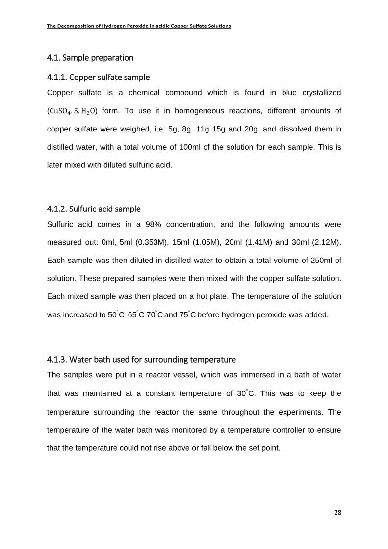
4.1. Sample preparation ........................................................................................... 28
4.1.1. Copper sulfate sample ................................................................................................28
4.1.2. Sulfuric acid sample ...................................................................................................28
4.1.3. Water bath used for surrounding temperature ...........................................................28
4.1.4. Addition of hydrogen peroxide ..................................................................................29
4.2. Reaction mechanism ......................................................................................... 30
4.2.1. The Reaction Vessel ..................................................................................................30
4.3. Temperature profile ........................................................................................... 31
4.3.1. The thermocouple sensitivity .....................................................................................31
4.3.2. Thermocouple calibration ..........................................................................................32
The Decomposition of Hydrogen Peroxide in acidic Copper Sulfate Solutions
vii
4.4. Data analysis .................................................................................................. 33
4.4.1. Coefficient of determination (R2) ..........................................................................34
4.4.2. Confidence intervals of parameters .......................................................................34
4.4.3. Error bars ...............................................................................................................35
5. Results and discussion ......................................................................................... 37
5.1. Introduction ...................................................................................................................37
5.1.2. The heat transfer coefficient for water .......................................................................38
5.2. The rate of decomposition of hydrogen peroxide .............................................. 42
5.2.1. The effect of temperature ...........................................................................................42
5.2.2. The effect of various environments on the decomposition of hydrogen peroxide 4748
5.2.3. The effects of varying volume of hydrogen peroxide ............................................5152
5.2.4. The effect of varying the amount of copper sulfate ...............................................5657
5.2.4.1. Effects of copper on reaction constant ............................................................ 6162
5.3. Model selection ............................................................................................. 6465
5.3.1. Confidence on the optimized parameters (𝐚, 𝐛) for model ....................................6768
The Endothermic Reaction ................................................................................... 6869
6. Conclusions ...................................................................................................... 7071
6.1.1. Effect of initial temperature ...................................................................................7071
6.1.2. Effects of reaction components on peroxide at 67C .............................................7172
6.1.3. Varying the volume of peroxide ............................................................................7172
6.1.4. The role of copper sulfate in the reaction ..............................................................7273
6.1.5. Rate determination .................................................................................................7273
6.2. Overall conclusion ......................................................................................... 7374
7. References ....................................................................................................... 7576
The Decomposition of Hydrogen Peroxide in acidic Copper Sulfate Solutions
viii
LIST OF FIGURES Figure 2.1: (a) is the graph of Cu2+-NH2OH-H2O2 system at constant initial concentration of
H2O2 and NH3OH+ with the concentration of Cu2+ varied, as a function of pH (Erlenmeyer,
Flierl and Sigel 1969); (b) is the evaluation of Figure 2.1.(a) at pH of 4.5. ............................... 13
Figure 2.2: The plot of the dependence of the initial rate on the concentration of copper
sulfate ( Perez-Benito 2001); main figure: [H2O2]0=0.196(empty circles)M and 0.392 (filled
circles and triangles) M, [KHPO4]=1.20(triangles) and 6.00(empty and filled circles) X10-2M,
pH=6.31(triangles) and 6.7 (empty and filled circles), [KNO3]=0(empty and filled circles) and
1.80 (triangles)M, at temperature of 25C,inset: initial rate in 10-7 circles,[KNO3]=2.64M) at
[H2O2]0=0.392M, [KH2PO4]=[K2HPO3]=1.20X10⁻² M, pH=6.16(circles) and 6.26 (triangles)
also at 25C ......................................................................................................................................... 15
Figure 4.1: The summarised flowchart of the experimental procedure. .................................... 27
Figure 4.2: This is the 3-dimensional image of the reaction vessel ........................................... 30
Figure 4.3: The rate at which the probe responds when immersed in two solutions of
different temperatures. ...................................................................................................................... 32
Figure 4.4: The graphical presentation of the temperature obtained from thermocouple and
thermometer. ....................................................................................................................................... 33
Figure 5.1: Temperature–time profile for the 250ml water contained in a batch reactor
cooling from an initial temperature of 67C which is immersed in a water batch at a controlled
temperature of 30 C. ......................................................................................................................... 39
Figure 5.2: The logarithm curve of the cooling water with an initial temperature of 67 C in a
water bath of 30 C. ............................................................................................................................ 40
Figure 5.3: Adiabatic temperature of the cooling water with initial temperature of 67 C. The
water bath temperature is 30C........................................................................................................ 41
The Decomposition of Hydrogen Peroxide in acidic Copper Sulfate Solutions
ix
Figure 5.4: Temperature–time profile of the 1.0 M solution of sulfuric acid and 0.3144M of
copper sulfate with 5ml of hydrogen peroxide injected at different initial temperatures (47C,
53C, 58 C and 67
C) with water bath at 30
C. ......................................................................... 4344
Figure 5.5: This displays the tail after 5 hours for the logarithm vs time curves of the solution
of 1.0M sulfuric acid and 0.3144M of copper sulfate with 5ml of peroxide at different initial
temperatures. Water bath is at 30C. .......................................................................................... 4445
Figure 5.6: The corrected (adiabatic) curves for the solution of 1.0M of sulfuric acid and
0.3144 M of copper sulfate and 5ml peroxide with initial temperature varying from 47C to
67C .................................................................................................................................................. 4647
Figure 5.7: The results of 5ml of peroxide decomposing in the presence of 250ml water
(red); 1.0M sulfuric acid (light green) and 0.3144M copper sulfate (purple). Pure water curve
(light blue) and the solution of CuSO4 and H2SO4 with 5ml H2O2 (Black). All at initial
temperature of 67C and total volume of 250ml. Water bath at 30
C. .................................... 4849
Figure 5.8: The linear plots of the cooling curves after five hours from Figure 5.7. ............. 4950
Figure 5.9: Corrected adiabatic curves from Figure 5.7 for the addition of 5ml solution of
peroxide in various media containing 1M sulfuric acid, 250ml water and 0.3144M copper
sulfate at initial temperature of 67C ........................................................................................... 5051
Figure 5.10: Temperature–time profile for 1.0 M of sulfuric acid,0.3144 M of copper sulfate
solutions at initial temperature of 67C . Volume of peroxide added: 0ml (purple), 5ml
(blue),15ml (dark red), 20ml (light green) and 30ml (light blue). Water bath temperature is
30C. ................................................................................................................................................. 5253
Figure 5.11: The linear plot of the tails of the curves from Figure 5.10 starting after 5h. .. 5354
Figure 5.12: The corrected adiabatic curves of the decomposition reaction of hydrogen
peroxide from the results in Figure 5.11. .................................................................................... 5455
The Decomposition of Hydrogen Peroxide in acidic Copper Sulfate Solutions
x
Figure 5.13: Graph of the temperature change versus the amount of peroxide added for the
results from Table 5.2. ................................................................................................................... 5657
Figure 5.14: The temperature–time profile for 1.0M sulfuric acid with 30ml hydrogen peroxide
added in the presence of different amount of copper sulfate: 0g (green), 5g (dark red), 8g
(light green), 11g (purple), 15g (light blue) and 20g (orange), all with initial temperature of
67C and the water bath was kept at 30
C . .............................................................................. 5758
Figure 5.15:The linear plot of the tail of the curves from Figure 5.14. ................................... 5859
Figure 5.16A: The corrected adiabatic curves of the results from Figure 5.14..................... 5960
Figure 5.16B: The adiabatic temperature rise plot from Figure 5.14 in which only the first 15
minutes duration is considered. ................................................................................................... 6061
Figure 5.17: The 𝐥𝐧𝐓∞− 𝐓𝐚𝐝 for the decomposition of hydrogen peroxide with different
amounts of copper sulfate against time. In this case 0g (Orange), 5g (Blue), 8g (Dark red),
11g (Light green), 15g (Purple) and 20g (Green) of copper sulfate is in solution with 1.0M
sulfuric acid and 30ml of peroxide is added. The experiments are done with an initial
temperature of 67 C. ..................................................................................................................... 6263
Figure 5.18: The graph of the change in mass of copper sulfate with the estimated first order
rate constant of the solution in which the mass of copper sulfate used was 0g, 5g, 8g, 11g,
15g and 20g in 1.0M of sulfuric acid at an initial temperature of 67C and with 30ml of
peroxide added. .............................................................................................................................. 6465
Figure 5.19: The graph of the amount of copper sulfate against the reaction rate constants
estimated in Figure 5.17 in comparison with the theoretical best fit model at a confidence
level of 95%. .................................................................................................................................... 6768
The Decomposition of Hydrogen Peroxide in acidic Copper Sulfate Solutions
xi
LIST OF TABLES Table. 5. 1: The linear trend line slopes from Figure 5.5 with their initial temperatures. .... 4546
Table 5.2: Change in the temperature between the initial and maximum temperature (rise) in
Figure 5.12, between the maximum and asymptotic temperature (drop) in Figure 5.12
together with the corresponding amount of peroxide added. .................................................. 5556
Table 5.3: The estimated rate constants with the corresponding amount of copper sulfate
added. .............................................................................................................................................. 6364
Table 5.4: Values of optimized parameters in Equation 5.2 computed at a confidence level of
95% .................................................................................................................................................. 6768
Table 5.5: Data for the plot of the mass of copper sulfate against estimated rate constant (k)
showing 95% error bands ............................................................................................................. 6869
The Decomposition of Hydrogen Peroxide in acidic Copper Sulfate Solutions
1
CHAPTER 1
1. Introduction
Chemical kinetics is one of the prerequisites for designing any production process
that includes chemical reactions. This study of reaction kinetics is governed by the
factors on which the rates of reaction depend, including the nature of the reactants
(acidic or basic), the amount of the reactants involved (which is known as the
concentration), the temperature of the system and pressure. The last of these,
pressure, can play an important role if the reaction system concerned uses
compressive mediums like gases (rather than liquids) or heterogeneous reactions.
In the metal recovery industries, kinetics are of vital use in processes involving
heterogeneous reactions between the metal deposited in solid ore and a liquid
lixiviate, resulting in dissolved metal and a by-product, normally an ionic salt. Such
processes are energy- and resource-intensive, and thus are responsible for a
significant portion of the costs of minerals processing plants. If the nature of the
reactions involved in the process is not thoroughly understood, then most of the
energy and materials required will be squandered. The important contribution
kinetics studies can make is to provide the knowledge necessary to optimizing the
process in question. This includes an understanding of the reaction mechanism, the
nature of the reactants, and their relation to the final product.
1.1. Statement of the problem
Most of the mineral leaching processes in common use involve a process with a
relatively slow reaction of several hours’ duration. One of the ways in which such
processes can be improved (and made more rapid) is to use oxidizing agents. Of the
The Decomposition of Hydrogen Peroxide in acidic Copper Sulfate Solutions
2
several types of oxidizing agent that have been considered for metal recovery, the
most common are air, chlorine and hydrogen peroxide (Haiyu, Jingyang and Jiakuan
2011; Olubambi, Borode and Ndlovu 2006).
Most mineral recovery plants find hydrogen peroxide the most suitable oxidant
because of its reaction products. It decomposes to water and oxygen, which makes it
eco-friendly (Li and Sheng 2008). Because it is in liquid form it is easier to handle
than oxygen/air, which is a cheaper oxidant than peroxide (Haiyu, Jingyang and
Jiakuan 2011). However, it has certain disadvantages that limit its use: it is
expensive, and it is not regenerable (Li and Sheng 2008), which implies that it
cannot be reused.
1.2. Research objectives
Our interest in the reaction kinetics for decomposition of hydrogen peroxide in
sulfuric acid solution with copper sulfate is the effects that the presence of copper
sulfate imposes on the peroxide in this system. These effects are studied using
temperature–time profile technique in an adiabatic batch reactor. The determination
of an empirical model relating the effects of mass of copper sulfate to the rate of
decomposition of hydrogen peroxide is also studied. The determination of this
relationship might be more easily understood when a better understanding of the
effect of temperature on the decomposition rate of peroxide and the contribution of
excess of peroxide in the solution is attained. If determined such knowledge might
have important consequences in the optimization of the use of peroxide in copper
leaching processes where sulfuric acid system is utilized.
The Decomposition of Hydrogen Peroxide in acidic Copper Sulfate Solutions
3
1.3. Structure of the dissertation
Chapter 2
In this chapter the writer provides an account of the discovery and significance of
hydrogen peroxide. The literature on the decomposition of peroxide is reviewed, and
particular attention is paid to description of the kinetic mechanism involved when the
peroxide is exposed to a catalytic reaction.
Chapter 3
The chapter starts by introducing the published work on temperature–time
measurements, and then sets out the equations derived from the batch reactor
energy and mass balances and discusses the correction required to take into
account the heat loss. The data is then corrected so that it is effectively models an
adiabatic batch reactor. The writer compares and discusses concentration–time and
temperature–time profiles for the various experimental conditions. The linear
dependency of the log of temperature versus time for the cooling curve is explained,
as is the estimation of the heat transfer coefficient of the system.
Chapter 4
This section describes the experimental apparatus and methods used, the
procedures followed and the variables measured.
Chapter 5
In this chapter the results obtained from the experiments are presented, discussed
and compared with the predictions arising from the theoretical analysis.
The Decomposition of Hydrogen Peroxide in acidic Copper Sulfate Solutions
4
Chapter 6
The conclusions derived from the analysis in the previous chapter are presented in
this chapter. The overall conclusion is based on the experimental findings and
evaluation of the data imparted by previous researchers.
The Decomposition of Hydrogen Peroxide in acidic Copper Sulfate Solutions
5
CHAPTER 2
2. Literature review
This chapter covers the discovery and manufacturing processes of hydrogen
peroxide. It presents the history of the manufacturing processes and the drawback
encountered in an attempt to advance those processes. The uses of peroxides are
further explained, with its contribution to environmental effects. The decomposition of
the peroxide is a function of its environment. This is significant in metal recovery.
2.1. The discovery and formation processes of hydrogen peroxide
Hydrogen peroxide was discovered in 1818 by a French chemist Louis Jacques
Thenard. He used the reaction of barium peroxide with nitric acid to produce a low
concentration of aqueous hydrogen peroxide (Strukul 1992). His process produced a
3% m/m solution of aqueous hydrogen peroxide. The production cost for this process
was high, therefore there was only a limited market. This was one of the major
disadvantages of its production. Later, in the year 1853, Meidinger discovered that
hydrogen peroxide can be produced from an electrochemical process using aqueous
sulfuric acid. The sulfuric acid in electrolysis was later replaced by ammonium
sulfate. By 1924 the annual production as a 100% m/m of aqueous hydrogen
peroxide had reached approximately 3.5X10⁶ kilograms. Further research on the
production processes of peroxide was conducted using different reactants, and with
tests such as the use of hydroquinones or hydrazobenzenes in alkaline conditions
(Jones 1999). Peroxide was produced from the treatment of hydroquinone with
oxygen, and also from the hydrogenation of an anthroquinone in the presence of a
catalyst. Another production process was the direct synthesis of hydrogen peroxide
The Decomposition of Hydrogen Peroxide in acidic Copper Sulfate Solutions
6
from H2 and O2 using a range of Au-Pd which was supported by alumina (Lunsford
2003; Solsona, et al. 2006; Yildiz and Akin 2007).
2.2. The uses of hydrogen peroxide
Hydrogen peroxide has been useful in various ways, from biological functions and
domestic uses to therapeutic uses (Abdollahi and Hosseini 2014). Although the
familiar use of peroxide for more than a century has been as a popular bleaching
agent (Beeman and Reichert 1953), this study investigates its use as an oxidizing
agent. This is due to the present industry focus on recovering metals.
2.2.1. The activation of hydrogen peroxide
In many applications the decomposition of hydrogen peroxide is an aided process
because it is a relatively weak oxidant. Especially when used alone in a mild
condition, it requires activation (Salem, El-Maazawi and Zaki 2000). The objective of
this activation is to increase its reactivity by converting peroxide into a different, more
active species (Strukul 1992).
One of the ways in which peroxide is activated is through radical decomposition. A
clear description is shown in Fenton’s reagent. In this case the iron catalyzes the
peroxides to generate a highly reactive species called hydroxyl radicals (OH∙)
(Schmidt, et al. 2011):
𝐇𝟐𝐎𝟐 + 𝐅𝐞𝟐+ → 𝐎𝐇 ∙ +𝐎𝐇− + 𝐅𝐞𝟑+ 𝟐. 𝟏
In situ chemical oxidation (ISCO) is an increasingly popular technology for the
treatment of contaminated soils. It is also based on this equation in which the highly
reactive hydroxyl radical rapidly reacts with most contaminants of concern (Buxton,
The Decomposition of Hydrogen Peroxide in acidic Copper Sulfate Solutions
7
et al. 1988; Haag and Yao 1992). ISCO includes catalyzed H2O2 propagation (CHP),
which differs slightly from Fenton’s reagent. The peroxide is used in a relatively high
concentration, together with alternative catalysts (e.g. iron (III), chelated iron, and
naturally occurring iron and manganese minerals). Other reactive oxygen species
are then generated through promotion of propagation reactions, namely, superoxide
anion (O2.-) and hydroperoxide anion (HO2
-).
𝐇𝟐𝐎𝟐 + 𝐎𝐇 ∙→ 𝐇𝐎𝟐 ∙ +𝐇𝟐𝐎 𝟐. 𝟐
𝐇𝟐𝐎𝟐 + 𝐅𝐞𝟑+ → 𝐇𝐎𝟐 ∙ +𝐇
+ + 𝐅𝐞𝟐+ 𝟐. 𝟑
𝐇𝐎𝟐 ∙↔ 𝐎𝟐 ∙−+𝐇+ 𝐩𝐊𝐚 = 𝟒. 𝟖 𝟐. 𝟒
𝐇𝐎𝟐 ∙ +𝐅𝐞𝟐+ → 𝐅𝐞𝟑+ +𝐇𝐎𝟐 ∙
− 𝟐. 𝟓
These oxygen species contribute to the CHP potential for rapid treatment of almost
all biorefractory compounds. However, its disadvantage lies in the rapid
decomposition of peroxide, which greatly reduces its effectiveness (Watts and Teel
2006).
The generation of metal peroxy or hydroperoxy species from the reaction of peroxide
and metal is also the mode of activation for H2O2 (Strukul 1992). This reaction is
essential to increase either the electrophilic or the nucleophilic character of the
peroxygens. An appropriate reaction for the formation of hydroperoxyl species is
found in the research investigating the decomposition of azo dye by the UV/H2O2
process (Chang, et al. 2010). Hydroxyl radicals that were generated by the UV
irradiation according to Equation 2.6 are being consumed to form hydroperoxyl
radical that has a lower oxidation capability, as shown in Equation 2.7
The Decomposition of Hydrogen Peroxide in acidic Copper Sulfate Solutions
8
𝐇𝟐𝐎𝟐 𝒉𝒗→ 𝟐𝐎𝐇 ∙ 𝟐. 𝟔
𝐇𝟐𝐎𝟐 + 𝐎𝐇 ∙→ 𝐇𝐎𝟐 ∙ +𝐇𝟐𝐎 𝟐. 𝟕
Thus the excess of peroxide favours the consumption of hydroxyl radicals and
decreases the dye reaction rate.
Croiset, Rice and Hanush (1997) studied the kinetics of the decomposition of
hydrogen peroxide in supercritical water. In their research they used supercritical
water oxidation (SCWO). This is a promising alternative technology for destroying
hazardous waste using the hydrothermal oxidation process. The technology is made
possible by the fact that above a critical point (at 374C and 22.1MPa) water causes
organic compounds (e.g. H2O2) to oxidize rapidly in a single phase. However, this
supercritical water experiment consumes a lot of energy in order to attain the high
temperatures required.
2.3. The metal recovering processes
In the process of recovering metals several methods have been found to be appropriate
and have been thoroughly investigated. The methods include mechanical processes,
pyrometallurgy and hydrometallurgy. Mechanical/physical processes are familiar separation
methods in the recycling industry though they cause dust emission and noise pollution, and
require tremendous energy usage (Li and Sheng 2008). Most importantly, the use of this
method has never recovered high purity metals. Pyrometallurgy uses high temperature
combustion to get the high temperatures required and, thus leads to serious air pollution.
Also, due to the smelters, like for copper, being located in remote areas away from urban
centres, the cost of the operation rises tremendously from energy consumption and
transportation of feedstock (Oishi, et al. 2007). Hydrometallurgy is a process in which metal

The Decomposition of Hydrogen Peroxide in acidic Copper Sulfate Solutions
9
contents are dissolved into leachants such as acids or alkalis (Olubambi and Potgieter
2009). This process has potentially lower costs and can be operated economically even on
a small scale (Li and Sheng 2008). Due to the flexibility, simplicity of operations and energy
saving, hydrometallurgical processing has become a substantial aspect of the metal
recovery industries.
Notwithstanding these positive features in hydrometallurgy, there have been drawbacks in
the operations of this process. These problems include low recovery of extracted metal and
difficulties in separating solids from liquids; in addition, the ease of purification is affected
by impurities (Olubambi and Potgieter 2009). The problem with for instance a sulfide ore in
hydrometallurgical processing is its low solubility in many leaching solutions. In principle it
was essential to simplify the dissolution of the constituent metal and an appropriate
leachant needed to be selected for the recovery of the targeted metal.
In assessing the dissolution capacity of a leaching reagent, the primary criteria for making
this selection are the cost and the effects that such a medium might have on the
environment. Previously, in the processes of copper leaching, several reagents have been
studied for their effectiveness in recovering this base metal. These reagents included the
following. Halogen salts of chlorides and bromides were studied by Stanley and
Subramanian (1977). Frankiewicz and Lueders (1979) researched using nitrogen dioxide
and chlorine gas-saturated water was studied by Ekinci, et al. (1998). All of these solutions
were used to recover copper from a chalcopyrite ore. However, these reagents are
relatively slow in the rate of recovering copper metal. They are also used in the removal of
other available metals such as zinc and iron. In 1998 the effectiveness of sulfuric acid
compared with hydrochloric acid, nitric acid, ferric chloride and ferrous sulfate was
reviewed by Prasad & Pandey (1998). In this study, nitric acid and hydrochloric acid were

The Decomposition of Hydrogen Peroxide in acidic Copper Sulfate Solutions
10
the most effective. However, both nitric acid and hydrochloric acid cause corrosion.
Therefore corrosion resistant equipment is required, but it is expensive.
Sulfuric acid is not as effective as other stronger oxidizing acids like nitric acid (Copur
2001; Copur 2002; Prasad and Pandey 1998). However, it is preferred to all other reagents
in terms of cost, corrosion wear and the ease of regeneration during electro winning
(Biswas and Davenport 1980). Besides, sulfuric acid is easily available and is a relatively
cheap reagent for base metal recovery (Antonijevic and Bogdanovic 2004). Therefore
optimization of sulfuric acid for a better recovery in leaching metals had to be considered.
2.3.1. Hydrogen peroxide in a sulfuric acid system for metal recovery
In assisting or optimizing the dissolution kinetics of sulfuric acid solution, hydrogen
peroxide became very useful. This is because peroxide is a strong oxidizing agent that
promotes the oxidation and leaching potential of the sulfuric acid system (Olubambi,
Borode and Ndlovu 2006). The leaching of ores/metals using sulfuric acid in conjunction
with hydrogen peroxide has been studied and successful results were obtained. The
dissolution kinetics of manganese-silver associated ores in the solution of H2SO4 and H2O2
were studied, and the recovery of silver was increased by the presence of hydrogen
peroxide (Tao, et al. 2002). In addition silver leaching was noted as diffusion controlled
with the kinetic model: 1-2x/3-(1-x) 2/3=kt (X is the mole fraction, t is the time (min), and k is
a mass transfer coefficient). The kinetics of the dissolution of chalcopyrite by hydrogen
peroxide in sulfuric acid was researched by Antonijevic, Dimitrijevic and Jankovic (1997) .
The presence of hydrogen peroxide with sulfuric acid again showed a significant increase
in the amount of copper recovered.
The Decomposition of Hydrogen Peroxide in acidic Copper Sulfate Solutions
11
Olubambi, Borode and Ndlovu (2006) also using the sulfuric and hydrogen peroxide
system, investigated the effectiveness of hydrogen peroxide as an oxidant. Their research
was on the leaching of zinc and copper from a Nigerian bulk sulfide ore. In this case they
observed that the leaching rate of zinc and copper increased with an increase in hydrogen
peroxide concentration. The dissolution kinetics of chalcopyrite in sulfuric acid and
hydrogen peroxide were also investigated by Adebayo, Impinmoroti and Ajayi (2003). They
found that the increase in stirring speed attributed to the faster decomposition of hydrogen
peroxide. They speculated that the molecular oxygen evolved is adsorbed onto the surface
of the chalcopyrite particles, and this hinders the contact between the particles and the
hydrogen peroxide solution.
2.3.2 Copper ions in a leaching solution of hydrogen peroxide and sulfuric acid
The leaching solution for copper metal recovery, using a sulfuric acid and hydrogen
peroxide system results in copper ions in solution with the remaining hydrogen
peroxide in diluted sulfuric acid. It is important to find out the nature of the
processes which take place in the remaining solution. There have been several
research studies on some combinations of this solution.
In the late 1960s Grant, Harwood and Wells (1968) reported that copper (Cu2+) in
solution contributes to the decomposition of hydrogen peroxide. That proceeds by a
combination of a molecular mechanism comprising the formation of free radicals
like HO2 and OH. Sigel, Flierl and Griesser (1969) confirmed the catalytic activity of
Cu2+ on hydrogen peroxide decomposition. They add that the activity of the catalyst
is a function of the concentration of the ligand of the copper ions. Their justification
lies in the activity of Cu2+-2, 2’-bipyridyl and Cu2+-2, 2’, 6’, 2’’terpyridyl.
The Decomposition of Hydrogen Peroxide in acidic Copper Sulfate Solutions
12
The kinetics and mechanism of the catalysis of the reaction between hydrogen
peroxide and hydrazine or hydroxylamine, by Cu2+ and Cu2+-2, and 2’-bipyridyl
complex, were also studied (Erlenmeyer, Flierl and Sigel 1969). This system was
represented by Equation 2.2 below:
𝟐𝐇𝟐𝐎𝟐 + 𝐍𝐇𝟐𝐍𝐇𝟐 → 𝐍𝟐 + 𝟒𝐇𝟐𝐎 𝟐. 𝟐
In this case it was discovered that in the decomposition of peroxide in the presence
of copper ion without a ligand, a precipitate was formed; the experiment was
therefore rendered difficult. However, the kinetics of the system was derived from
the proportionality of the initial velocity of the decreasing concentration of H2O2 to
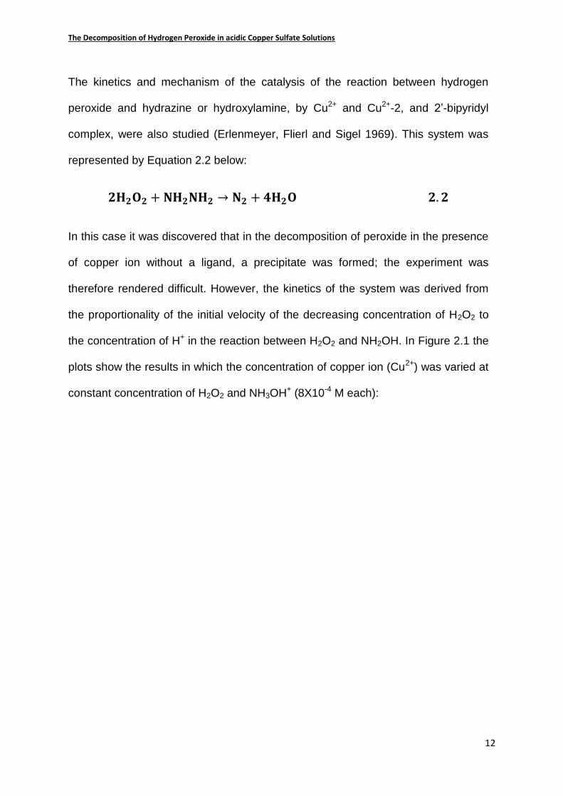
the concentration of H+ in the reaction between H2O2 and NH2OH. In Figure 2.1 the
plots show the results in which the concentration of copper ion (Cu2+) was varied at
constant concentration of H2O2 and NH3OH+ (8X10⁻⁴ M each):
The Decomposition of Hydrogen Peroxide in acidic Copper Sulfate Solutions
13
Figure 2.1: (a) is the graph of Cu2+-NH2OH-H2O2 system at constant initial
concentration of H2O2 and NH3OH+ with the concentration of Cu2+ varied, as a
function of pH (Erlenmeyer, Flierl and Sigel 1969); (b) is the evaluation of Figure
2.1.(a) at pH of 4.5.
Onuchukwu (1984) used copper and nickel ferrites to study the heterogeneous
catalytic decomposition of hydrogen peroxide. The findings revealed that under the
same experimental conditions the activity of copper superseded that of the nickel
catalyst. This shows that copper is a better catalyst in decomposing peroxide than
nickel. Furthermore the decomposition of peroxide in potassium hydroxide (KOH)
obeyed the first order rate equation with respect to total hydrogen peroxide content;
such a trend concurred with several reports of previous authors for peroxide
decomposition in an alkaline media.
The catalytic action of copper (II) on the hydrogen peroxide decomposition which is
in near neutrality aqueous solution is activated by halide ions (Perez-Benito 2001).
Though the effect of fluorine (F-) ion could only be studied at relatively low
The Decomposition of Hydrogen Peroxide in acidic Copper Sulfate Solutions
14
concentrations (up to 0.360M), its increase in concentration contributes to an
increase in pH. This is caused by the formation of HF, which is a weaker acid than
the other hydrogen halides. Thus the activation effect of the halide ions was found to
follow this sequence: Cl>F>Br. KCl was more efficient as activator of the catalyst
while KBr- had an inhibiting effect. However, I- yielded a precipitate Cu2I2 when
reacting with Cu (II) which affects the homogeneity of the solution.
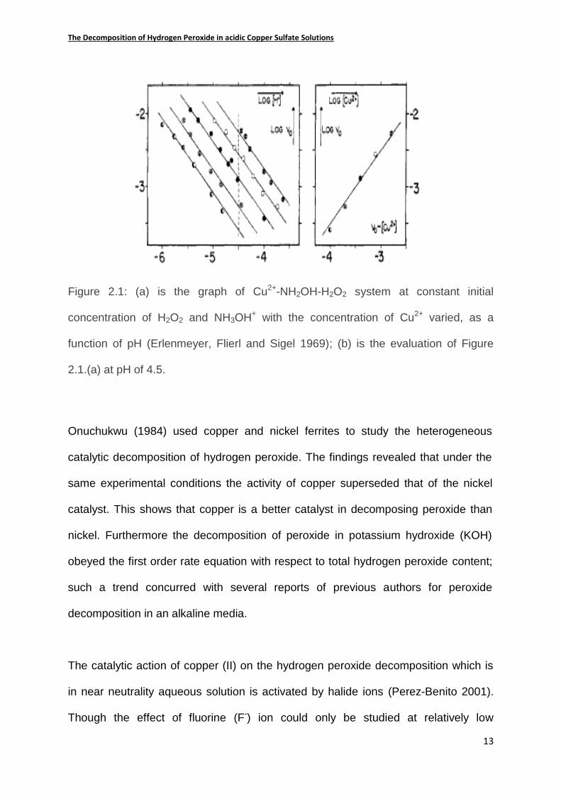
Figure 2.2 shows the effect of the increment of Cu (II) on the decomposition of
peroxide in the presence of the solution constituents. The inset graph displayed the
effect of Cu (II) on the rate constant. It is worth noting that at [Cu (II)] =0M, the graph
has a zero coordinate, which implies that copper ion is the driving force behind the
decomposition of hydrogen peroxide
The Decomposition of Hydrogen Peroxide in acidic Copper Sulfate Solutions
15
Figure 2.2: The plot of the dependence of the initial rate on the concentration of
copper sulfate ( Perez-Benito 2001); main figure: [H2O2]0=0.196(empty circles)M and
0.392 (filled circles and triangles) M, [KHPO4]=1.20(triangles) and 6.00(empty and
filled circles) X10-2M, pH=6.31(triangles) and 6.7 (empty and filled circles),
[KNO3]=0(empty and filled circles) and 1.80 (triangles)M, at temperature of
25C,inset: initial rate in 10-7 circles,[KNO3]=2.64M) at [H2O2]0=0.392M,
[KH2PO4]=[K2HPO3]=1.20X10⁻² M, pH=6.16(circles) and 6.26 (triangles) also at 25C
2.3.3 The reaction kinetics for Hydrogen peroxide decomposition in a sulfuric acid
system
The reaction kinetics for hydrogen peroxide decomposition has been studied for a
long time especially with respect to catalytic decomposition using transition metals
(Haber and Weiss 1934; Sigel, Flierl and Griesser 1969; Kanungo, Parida and Sant
1981; Borrull and Cerda 1987; Strukul 1992). Due to the increasing interest in the
use of hydrogen peroxide as an oxidant for specific organic transformations, it

The Decomposition of Hydrogen Peroxide in acidic Copper Sulfate Solutions
16
seems suitable to review the research based on transition metal catalyzed oxidation
especially with copper which is the metal of interest for this research. Nevertheless,
what is significant is the researchers’ findings, the procedures which were followed
in studying the kinetics and the relevance of their findings relevant to our research
studies.
In the study of the kinetics of hydrogen peroxide decomposition the measuring of the
initial velocity, vo, of the decreasing concentration of H202 with temperature at 25C
was used (Erlenmeyer, Flierl and Sigel 1969; Sigel, Flierl and Griesser 1969).
Kanungo, Parida and Sant (1981) similarly studied the kinetics of peroxide; however,
they considered the oxygen liberated as the H2O2 decomposed at various
temperatures (20C -40C). Borrull and Cerda (1987) used temperature–time profiles
while Jiang et al. (2002) and Choudhary and Gaikwad (2003) considered the
relationship between the rate of reaction and the concentration of the reactants at
various temperatures 8oC-40C and 30C –60C respectively.
So far the kinetics of sulfuric acid and peroxide system had been studied relating
their concentrations with the rate of the reacting metal (Antonijevic and Bogdanovic
2004). Also the effect of copper ions in solution had been shown by previous
researchers to promote catalytic decomposition. Furthermore, peroxide had been
recommended in the metal recovery industries rather than other oxidants.
However, in the previous research findings a gap remained unfilled as far as the
leaching of metal using peroxide is concerned, which prompted the current
research. First of all, though the sulfuric acid system had been examined, the effect
of the copper concentration on the peroxide decomposition was still to be
investigated. This was because the report on the effects of copper ions on the

The Decomposition of Hydrogen Peroxide in acidic Copper Sulfate Solutions
17
peroxide was based on a different system and no thorough research had been
done. The present research looks at the effect of copper in solution on the
hydrogen peroxide decomposition.
The Decomposition of Hydrogen Peroxide in acidic Copper Sulfate Solutions
18
CHAPTER 3
3. The description of the temperature–time technique
This chapter provides a contextual background on the use of temperature–time
profiles for kinetic analysis of chemical reaction processes. It explains the theory
behind the analysis of the measured temperature versus time profiles, and sets out
the relevant equations derived from the mass and energy balances in a batch reactor
system. It also explains the writer’s reasons for choosing to use this method. The
measured temperature–time profiles were corrected for heat loss so as to predict the
effective temperature vs time curves that would have been measured if the reactor
was adiabatic. This allows us to relate the corrected adiabatic temperature to the
reaction conversion which allows us to determine the reaction kinetics
3.1. Adiabatic batch reactor measurement
Although continuous (flow) reactors are dominant in the chemical industry (Schmidt
1998), a batch reactor is preferable for experiments undertaken at the laboratory
scale. It is worth noting that the equations describing batch and plug flow tubular
reactors are very similar (Schmidt 1998). Previous researchers (Hartridge and
Roughton 1924) utilized temperature profiles for an improved apparatus for
measuring the velocity of very rapid chemical reactions. To enhance their
understanding of this apparatus, they also used the neutralization of sodium
hydroxide and monitored the time it takes to reach completion (calling it the
theoretical temperature rise). However, a flow reactor has been generally used for
fast reactions (La Mer and Read 1930).

The Decomposition of Hydrogen Peroxide in acidic Copper Sulfate Solutions
19
Dyne, Glasser and King (1967) studied reaction rates using an automatically
controlled adiabatic reactor using temperature-time measurements. In this
experiment, the wall temperature was maintained at the same level as that of the
mixture in the reactor by means of a direct heating current, thereby making the
reactor effectively adiabatic.
In the study of homogeneous liquid phase kinetics, also carried out in a batch
reactor, Glasser and Williams (1971) considered temperature as a variable against
time. In this case, the kinetic parameters were obtained by means of regression
analysis, using the corrected experimental temperature–time curve. It is worth noting
that regression analysis is appropriate when the concentration of the contents and
the temperature are varied simultaneously, and therefore can be expressed by the
differential equation 3.1 (Scott, Glasser and Nicol 1975).
∆𝐇𝐫𝐱𝐧𝒅𝒙
𝒅𝒕= 𝐔𝐀(𝑻 − 𝑻𝒔) + 𝐌𝐂𝐏
𝒅𝑻
𝒅𝒕− 𝑸 𝟑. 𝟏
where:
∆𝐻𝑟𝑥𝑛 is the heat of reaction
x is the extent of reaction
𝑀 is the total mass of the reactor and its contents
𝐶𝑃 is the heat capacity of the reactor and the contents
𝑄 is the rate of heat generated by the mechanical stirrer
𝑈 is the heat transfer coefficient between the contents of reactor and the
surroundings
𝑇 is the temperature of the contents of the reactor
The Decomposition of Hydrogen Peroxide in acidic Copper Sulfate Solutions
20
𝑇𝑆 is the temperature of the surroundings; and
𝐴 is the external area of the reactor, corresponding to the surface through which
heat transfer between the reactor and the surroundings occurs.
In order to ensure that the heat loss to the surroundings could be controlled and
modelled, the reactor was placed in a constant temperature bath so that the
temperature of the surroundings was constant.
The technique developed by Glasser and Williams (1971) for the estimation of the
rate of reaction for a homogeneous reaction is known as the classical method. In
this research the temperature of the walls of the reactor was automatically
controlled in order to keep the temperature of the walls the same as that of the
contents. Most importantly, the classical method enabled the temperature–time
curve to be converted directly into concentration versus time data. The data can
therefore be analyzed to determine reaction kinetics. Notwithstanding, there was
discrepancy at higher temperature, which they presumed was attributable to their
having halted the reaction from time to time to take samples for concentration
measurement. This might have diminished the accuracy obtainable by the classical
method.
3.2. Mathematical Analysis of Adiabatic batch system
Heat is released (or absorbed) when a reaction occurs, and this leads to an increase
(decrease) in temperature in an adiabatic reactor. The differential equation
appropriate to such curves is derived from the combination of the mass and energy
balance for the reaction and the following assumptions:
The law of mass and energy conservation
The Decomposition of Hydrogen Peroxide in acidic Copper Sulfate Solutions
21
The Arrhenius equation described the temperature dependence of reaction
rates;
that the heat change is almost entirely attributable to a single reaction;
that the heat of reaction is not a function of temperature; and
the specific heat of the system is independent of temperature and composition
of the reacting mixture.
The equation of the mass balance can be related to that of the energy balance.
There is proportionality between the temperature of the single reaction and its extent
of reaction. This results in a differential equation in terms of temperature–time
variations for an adiabatic system. This is shown in section 3.3 below.
3.3. The energy balance equation for adiabatic batch reactor
In this section, the derivation of the equation produced from energy and mass
balance, which relates the kinetics and thermodynamic parameters of a reaction, is
set out. The relationship between reaction kinetics and the temperature of the
reacting constituents is explicitly defined.
A batch reactor that is perfectly mixed, meaning that the concentration of the
reacting constituents is spatially uniform (Fogler 1999), has the molar balance in
terms of the concentration of the reactant:
−𝐫𝐀 = −𝟏
𝐕
𝐝𝐍𝐀𝐝𝐭 = −
𝐝𝐂𝐀𝐝𝐭 (𝟑. 𝟐. )
where −𝑟𝐴 is the rate of formation of species A
V is the volume of the reacting solution
The Decomposition of Hydrogen Peroxide in acidic Copper Sulfate Solutions
22
NA is the moles of A in the reacting solution
t is time
CA is the concentration of reactant A in the solution.
The energy balance around a reactor can be clearly expressed through the
consideration of these terms:
o the energy produced by the reactants;
o the energy generated by the mechanical stirrer in mixing the solution;
o the absorbed energy by the reactor contents;
o the energy due to heat transfer to the surrounding through the reactor walls.
Thus for a small time interval the mathematical equation relates the energy
generated with that absorbed and released for a steady state process according to
Equation 3.3:
(−∆𝐇𝐫𝐱𝐧)(−𝐫𝐀)𝐕𝐝𝐭 + 𝐐𝐬𝐝𝐭 = 𝐌𝐂𝐩𝐝𝐓 + 𝐔𝐀(∆𝐓)𝐝𝐭 (𝟑. 𝟑)
Shatynski and Hanesian (1993) considered the heat due to stirring in Equation 3.3
( Qsdt ) to be negligible, and this is the assumption considered in this investigation
since according to them compared to the other terms of Equation 3.3, it is relatively
small. The remaining equation becomes:
(−∆𝐇𝐫𝐱𝐧)(−𝐫𝐀)𝐕𝐝𝐭 = 𝐌𝐂𝐩𝐝𝐓 + 𝐔𝐀(∆𝐓)𝐝𝐭 (𝟑. 𝟒)
since also in terms of extent of reaction the rate equation can be written thus:
(−𝒓𝑨 )𝑽 = 𝒅𝜺
𝒅𝒕 = rate of reaction (𝟑. 𝟓)
In this case 𝛆 is the extent of reaction.
Therefore Equation 3.5 is substituted into Equation 3.4 to yield Equation 3.6:
The Decomposition of Hydrogen Peroxide in acidic Copper Sulfate Solutions
23
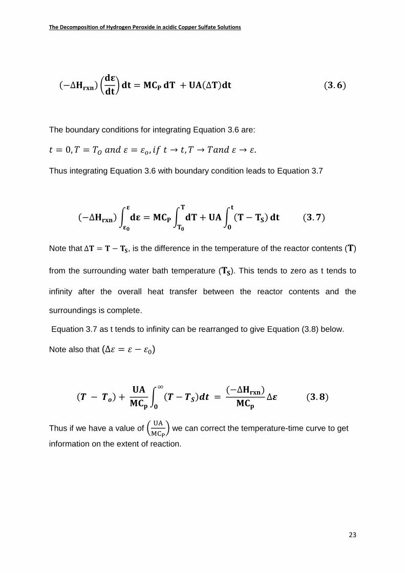
(−∆𝐇𝐫𝐱𝐧) (𝐝𝛆
𝐝𝐭)𝐝𝐭 = 𝐌𝐂𝐏 𝐝𝐓 + 𝐔𝐀(∆𝐓)𝐝𝐭 (𝟑. 𝟔)
The boundary conditions for integrating Equation 3.6 are:
𝑡 = 0, 𝑇 = 𝑇𝑂 𝑎𝑛𝑑 𝜀 = 𝜀𝑜, 𝑖𝑓 𝑡 → 𝑡, 𝑇 → 𝑇𝑎𝑛𝑑 𝜀 → 𝜀.
Thus integrating Equation 3.6 with boundary condition leads to Equation 3.7
(−∆𝐇𝐫𝐱𝐧)∫ 𝐝𝛆𝛆
𝛆𝟎
= 𝐌𝐂𝐏∫ 𝐝𝐓𝐓
𝐓𝟎
+ 𝐔𝐀∫ (𝐓 − 𝐓𝐒)𝐭
𝟎
𝐝𝐭 (𝟑. 𝟕)
Note that ∆𝐓 = 𝐓 − 𝐓𝐒, is the difference in the temperature of the reactor contents (𝐓)
from the surrounding water bath temperature (𝐓𝐒). This tends to zero as t tends to
infinity after the overall heat transfer between the reactor contents and the
surroundings is complete.
Equation 3.7 as t tends to infinity can be rearranged to give Equation (3.8) below.
Note also that (∆𝜀 = 𝜀 − 𝜀0)
(𝑻 − 𝑻𝒐) + 𝐔𝐀
𝐌𝐂𝐩∫ (𝑻 − 𝑻𝑺)𝒅𝒕 =
(−∆𝐇𝐫𝐱𝐧)
𝐌𝐂𝐩∆𝜺
∞
𝟎
(𝟑. 𝟖)
Thus if we have a value of (UA
MCP) we can correct the temperature-time curve to get
information on the extent of reaction.
The Decomposition of Hydrogen Peroxide in acidic Copper Sulfate Solutions
24
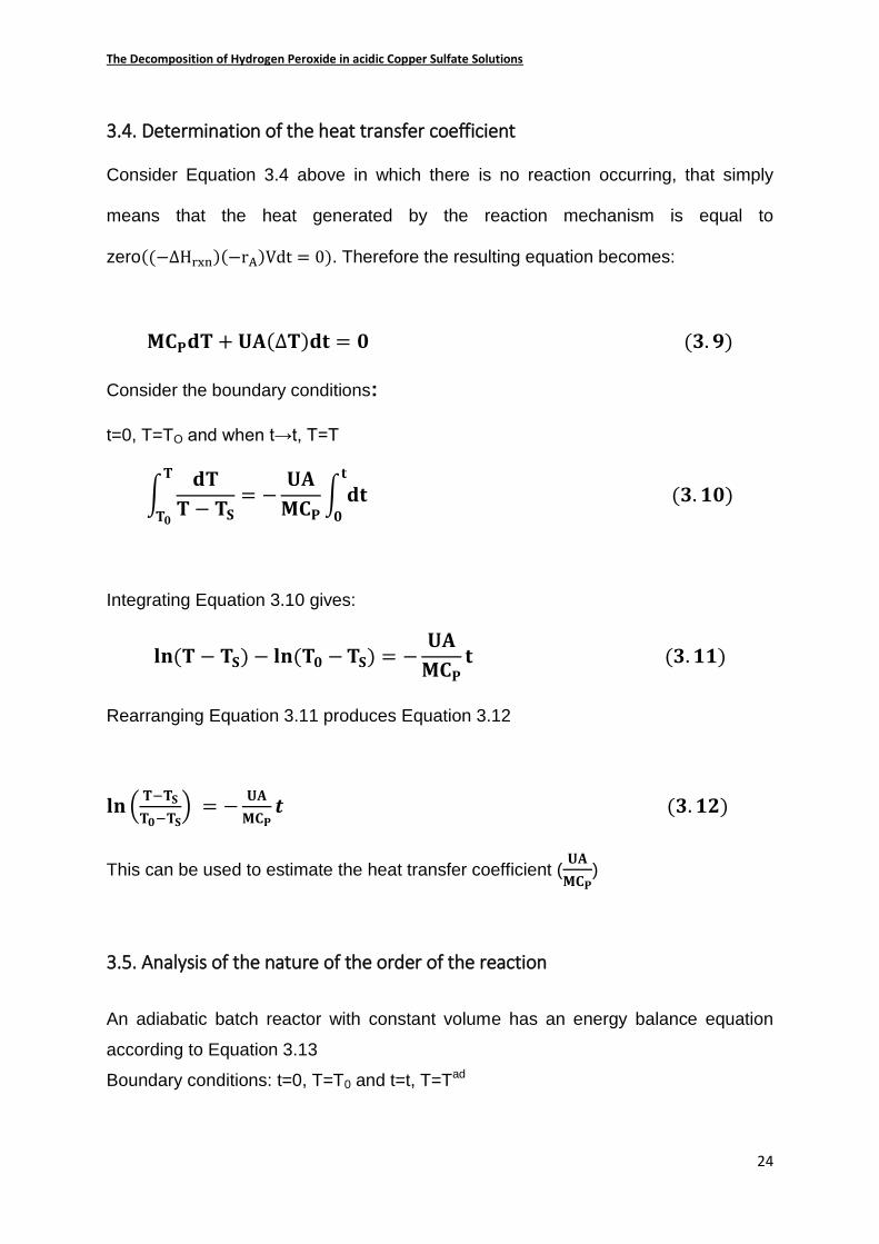
3.4. Determination of the heat transfer coefficient
Consider Equation 3.4 above in which there is no reaction occurring, that simply
means that the heat generated by the reaction mechanism is equal to
zero((−∆Hrxn)(−rA)Vdt = 0). Therefore the resulting equation becomes:
𝐌𝐂𝐏𝐝𝐓 + 𝐔𝐀(∆𝐓)𝐝𝐭 = 𝟎 (𝟑. 𝟗)
Consider the boundary conditions:
t=0, T=TO and when t→t, T=T
∫𝐝𝐓
𝐓 − 𝐓𝐒
𝐓
𝐓𝟎
= −𝐔𝐀
𝐌𝐂𝐏∫ 𝐝𝐭𝐭
𝟎
(𝟑. 𝟏𝟎)
Integrating Equation 3.10 gives:
𝐥𝐧(𝐓 − 𝐓𝐒) − 𝐥𝐧(𝐓𝟎 −𝐓𝐒) = −𝐔𝐀
𝐌𝐂𝐏𝐭 (𝟑. 𝟏𝟏)
Rearranging Equation 3.11 produces Equation 3.12
𝐥𝐧 (𝐓−𝐓𝐒
𝐓𝟎−𝐓𝐒) = −
𝐔𝐀
𝐌𝐂𝐏𝒕 (𝟑. 𝟏𝟐)
This can be used to estimate the heat transfer coefficient (𝐔𝐀
𝐌𝐂𝐏)
3.5. Analysis of the nature of the order of the reaction
An adiabatic batch reactor with constant volume has an energy balance equation
according to Equation 3.13
Boundary conditions: t=0, T=T0 and t=t, T=Tad

The Decomposition of Hydrogen Peroxide in acidic Copper Sulfate Solutions
25
𝐌𝐂𝐩 𝐝𝐓𝒂𝒅
𝐝𝐭= (−∆𝐇𝐑𝐱𝐧)(−𝒓𝑨𝑽) (𝟑. 𝟏𝟑)
For a perfectly insulated batch reactor no heat loss occurs and (Tad) is the difference
between the temperature in the adiabatic reactor at time t and the temperature in the
reactor initially.
For a constant volume reaction, the rate equation in terms of concentration is written
in this way (see Equation 3.2):
𝐫𝐀 =𝐝𝐂𝐀
𝐝𝐭 (𝟑. 𝟏𝟒)
Note that A represents a reactant, thus CA is the concentration of A and rAthe rate
of formation of A. Now substituting equation 3.14 in 3.13 leads to Equation 3.15
below:
𝐌𝐂𝐏𝐝(𝐓𝐚𝐝)
𝐝𝐭=∆𝐇𝐫𝐱𝐧𝐕𝐝𝐂𝐀
𝐝𝐭 (𝟑. 𝟏𝟓)
Now rearranging Equation 3.15 gives Equation 3.16:
𝐝(𝐓𝐚𝐝)
𝐝𝐂𝐀=∆𝐇𝐑𝐱𝐧𝐕
𝐌𝐂𝐏 (𝟑. 𝟏𝟔)
To integrate Equation 3.16 the boundary condition should be specified.
Boundary conditions: at t= 0, T (0) =TO and CA (0) =CAO; at t=t, T (t) =Tad CA (t) =CA
∫ 𝐝(𝐓𝐚𝐝)𝐓𝐚𝐝
𝐓𝟎
=∆𝐇𝐫𝐱𝐧𝐕
𝐌𝐂𝐏∫ 𝐝𝐂𝐀
𝐂𝐀
𝐂𝐀𝐨
(𝟑. 𝟏𝟕)
Therefore Equation 3.17 gives Equation 3.18:
The Decomposition of Hydrogen Peroxide in acidic Copper Sulfate Solutions
26
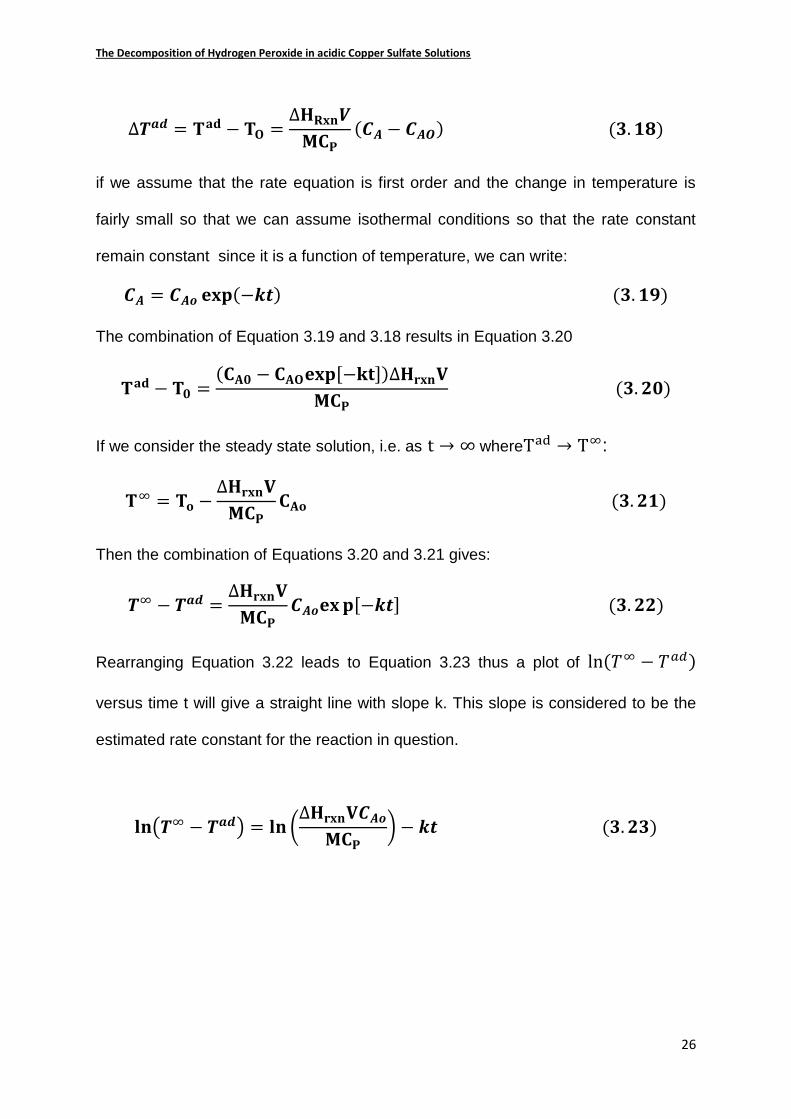
∆𝑻𝒂𝒅 = 𝐓𝐚𝐝 − 𝐓𝐎 =∆𝐇𝐑𝐱𝐧𝑽
𝐌𝐂𝐏(𝑪𝑨 − 𝑪𝑨𝑶) (𝟑. 𝟏𝟖)
if we assume that the rate equation is first order and the change in temperature is
fairly small so that we can assume isothermal conditions so that the rate constant
remain constant since it is a function of temperature, we can write:
𝑪𝑨 = 𝑪𝑨𝒐 𝐞𝐱𝐩(−𝒌𝒕) (𝟑. 𝟏𝟗)
The combination of Equation 3.19 and 3.18 results in Equation 3.20
𝐓𝐚𝐝 − 𝐓𝟎 =(𝐂𝐀𝟎 − 𝐂𝐀𝐎𝐞𝐱𝐩[−𝐤𝐭])∆𝐇𝐫𝐱𝐧𝐕
𝐌𝐂𝐏 (𝟑. 𝟐𝟎)
If we consider the steady state solution, i.e. as t → ∞ whereTad → T∞:
𝐓∞ = 𝐓𝐨 −∆𝐇𝐫𝐱𝐧𝐕
𝐌𝐂𝐏𝐂𝐀𝐨 (𝟑. 𝟐𝟏)
Then the combination of Equations 3.20 and 3.21 gives:
𝑻∞ − 𝑻𝒂𝒅 =∆𝐇𝐫𝐱𝐧𝐕
𝐌𝐂𝐏𝑪𝑨𝒐𝐞𝐱𝐩[−𝒌𝒕] (𝟑. 𝟐𝟐)
Rearranging Equation 3.22 leads to Equation 3.23 thus a plot of ln(𝑇∞ − 𝑇𝑎𝑑)
versus time t will give a straight line with slope k. This slope is considered to be the
estimated rate constant for the reaction in question.
𝐥𝐧(𝑻∞ − 𝑻𝒂𝒅) = 𝐥𝐧 (∆𝐇𝐫𝐱𝐧𝐕𝑪𝑨𝒐𝐌𝐂𝐏
) − 𝒌𝒕 (𝟑. 𝟐𝟑)
The Decomposition of Hydrogen Peroxide in acidic Copper Sulfate Solutions
27
CHAPTER 4
4. Experimental section
This chapter outlines the mode in which experimental data was brought together and
also explains the apparatus that was used to perform the experiments. The focus of
these experiments was on the hydrogen peroxide decomposing in copper leaching
solution. According to the display of Equation 4.1 (Khandpur 2005) the dissolution of
copper in sulfuric acid solution, with peroxide as an oxidant, yields a metal salt called
copper sulfate, and water:
𝐂𝐮 + 𝐇𝟐𝐒𝐎𝟒 +𝐇𝟐𝐎𝟐 → 𝐂𝐮𝐒𝐎𝟒 + 𝟐𝐇𝟐𝐎 𝟒. 𝟏
In order to maintain a high reaction rate most industrial processes normally run with
an excess of the reagent. Because of this excess of reactant/s, the final solution can
still contain unreacted reagents. Thus these experiments were performed with an
excess of the reagents in the solution. The solution prepared comprised dissolved
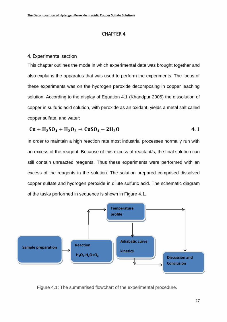
copper sulfate and hydrogen peroxide in dilute sulfuric acid. The schematic diagram
of the tasks performed in sequence is shown in Figure 4.1.
Figure 4.1: The summarised flowchart of the experimental procedure.
Adiabatic curve
kinetics Sample preparation
Reaction
H2O2-H2O+O2
Temperature
profile
Discussion and
Conclusion
The Decomposition of Hydrogen Peroxide in acidic Copper Sulfate Solutions
28
4.1. Sample preparation
4.1.1. Copper sulfate sample
Copper sulfate is a chemical compound which is found in blue crystallized
(CuSO4. 5. H2O) form. To use it in homogeneous reactions, different amounts of
copper sulfate were weighed, i.e. 5g, 8g, 11g 15g and 20g, and dissolved them in
distilled water, with a total volume of 100ml of the solution for each sample. This is
later mixed with diluted sulfuric acid.
4.1.2. Sulfuric acid sample
Sulfuric acid comes in a 98% concentration, and the following amounts were
measured out: 0ml, 5ml (0.353M), 15ml (1.05M), 20ml (1.41M) and 30ml (2.12M).
Each sample was then diluted in distilled water to obtain a total volume of 250ml of
solution. These prepared samples were then mixed with the copper sulfate solution.
Each mixed sample was then placed on a hot plate. The temperature of the solution
was increased to 50C, 65C 70C and 75C before hydrogen peroxide was added.
4.1.3. Water bath used for surrounding temperature
The samples were put in a reactor vessel, which was immersed in a bath of water
that was maintained at a constant temperature of 30C. This was to keep the
temperature surrounding the reactor the same throughout the experiments. The
temperature of the water bath was monitored by a temperature controller to ensure
that the temperature could not rise above or fall below the set point.
The Decomposition of Hydrogen Peroxide in acidic Copper Sulfate Solutions
29
4.1.4. Addition of hydrogen peroxide
In all the experiments performed, the hydrogen peroxide used was 30% in
concentration. Peroxide was injected at room temperature into the reactor by means
of a syringe with a volume of 50ml. The amounts injected were 0ml, 5ml, 15ml, 20ml
and 30ml, depending on the experiment.
The details of the solution components used are summarized in Table 4.1 below. In
this case the molarity of each component is included.
Table 4.1: The concentration and the amounts of the components that were used for
the experiments
Copper sulfate Hydrogen peroxide
grams
in
250ml
MW Conc% ml in
250ml
MW Conc%
250 100 34 30
moles moles/l moles moles/l
5 20 80 5 44 176
8 32 128 15 132 529
11 44 176 20 176 706
15 60 240 30 265 1059
20 80 320
The Decomposition of Hydrogen Peroxide in acidic Copper Sulfate Solutions
30
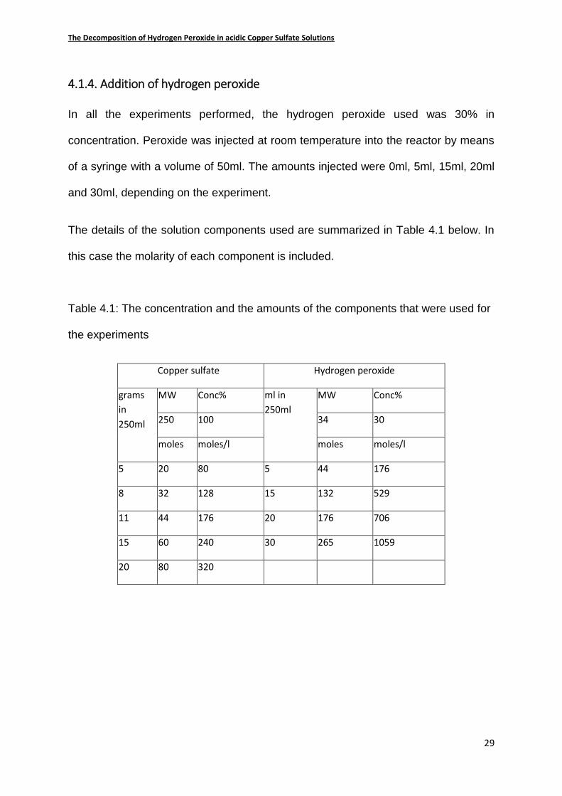
4.2. Reaction mechanism
4.2.1. The Reaction Vessel
The reaction vessel used was a 500ml thermos flask with a removable cap lid made
of expanded polystyrene to minimize heat losses. The lid was pierced to make two
holes small enough to allow a probe and syringe to be passed through. Stirring was
carried out in the flask by means of a magnetic stirrer. Figure 4.2 is a photograph of
the flask used.
Figure 4.2: This is the 3-dimensional image of the reaction vessel
A heated solution of sulfuric acid and copper sulfate was poured into the reaction
vessel, and a temperature probe was inserted through the lid. The temperature
recorded by the probe was displayed on the computer monitor. The temperature in
the reaction vessel was allowed to stabilize prior to the addition of peroxide.
Hydrogen peroxide was then slowly injected through the second hole to avoid the
formation of bubbles inside the reactor.
Reactor vessel
Polystyrene lid
The Decomposition of Hydrogen Peroxide in acidic Copper Sulfate Solutions
31
The hydrogen peroxide was introduced at room temperature. The temperature of the
solution in the reactor dropped relative to the amount of the oxidant used. The nature
of the reaction that follows determines the resultant temperature of the solution: an
exothermic reaction has a positive temperature gradient, while an endothermic
reaction has a negative gradient. The pH of the solution was not considered an
important parameter in these experiments.
4.3. Temperature profile
4.3.1. The thermocouple sensitivity
Sulfuric acid is a very strong acid which reacts with most metals. Since the
thermocouple (type K) used is chromel/alumel (metallic) (Wang 1990), it is sheathed
in a blown glass container to act as an insulator against the acidity of the solution.
However, as the air surrounding the thermocouple inside the glass reduces the
sensitivity of the thermocouple, a small amount of water was poured into the glass to
increase the contact surface between the glass and the thermocouple. This
insulation sheath caused a delay in the measurement by the thermocouple when it
was inserted into the medium.
The thermocouple was immersed in two media, each of a different temperature, in
order to measure the delay of the response. In the first instance, this device was
immersed in tap water at 20C. After three minutes it was removed and immediately
afterwards plunged into a mixture of water and crushed ice at a temperature of 0C.
The temperature detected by the probe dropped from 20C to -0.008C in just under
four minutes, as shown in Figure 4.3. The Figure shows that the probe took
approximately 20 seconds to read the temperature of the new medium, it follows that
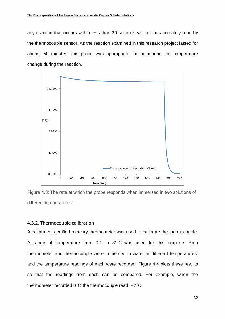
The Decomposition of Hydrogen Peroxide in acidic Copper Sulfate Solutions
32
any reaction that occurs within less than 20 seconds will not be accurately read by
the thermocouple sensor. As the reaction examined in this research project lasted for
almost 50 minutes, this probe was appropriate for measuring the temperature
change during the reaction.
Figure 4.3: The rate at which the probe responds when immersed in two solutions of
different temperatures.
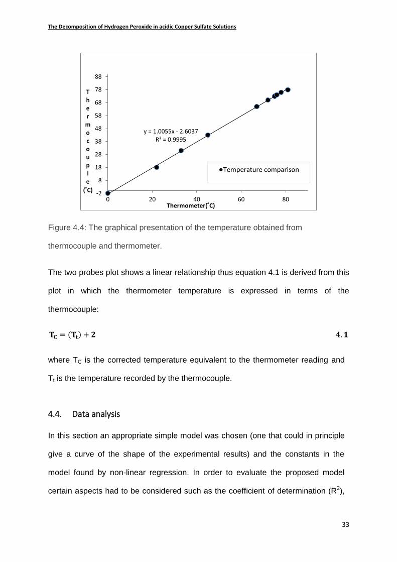
4.3.2. Thermocouple calibration
A calibrated, certified mercury thermometer was used to calibrate the thermocouple.
A range of temperature from 0C to 81C was used for this purpose. Both
thermometer and thermocouple were immersed in water at different temperatures,
and the temperature readings of each were recorded. Figure 4.4 plots these results
so that the readings from each can be compared. For example, when the
thermometer recorded 0 C, the thermocouple read ~-2 C.
The Decomposition of Hydrogen Peroxide in acidic Copper Sulfate Solutions
33
Figure 4.4: The graphical presentation of the temperature obtained from
thermocouple and thermometer.
The two probes plot shows a linear relationship thus equation 4.1 is derived from this
plot in which the thermometer temperature is expressed in terms of the
thermocouple:
𝐓𝐂 = (𝐓𝐭) + 𝟐 𝟒. 𝟏
where TC is the corrected temperature equivalent to the thermometer reading and
Tt is the temperature recorded by the thermocouple.
4.4. Data analysis
In this section an appropriate simple model was chosen (one that could in principle
give a curve of the shape of the experimental results) and the constants in the
model found by non-linear regression. In order to evaluate the proposed model
certain aspects had to be considered such as the coefficient of determination (R2),
y = 1.0055x - 2.6037 R² = 0.9995
-2
8
18
28
38
48
58
68
78
88
0 20 40 60 80
T h e r
m o c o u p l e
(C)
Thermometer(C)
●Temperature comparison
The Decomposition of Hydrogen Peroxide in acidic Copper Sulfate Solutions
34
confidence interval and error bars to know how scientifically plausible values the
best fit values are.
4.4.1. Coefficient of determination (R2)
By definition the coefficient of determination (R2) is considered as the amount of the
variation in the dependent variable that is explained by the regression line in terms
of the predictor variable (Katubilwa 2012). This in short is used to quantify the
goodness of the proposed model to the experimental data fit. As the rule of thumb a
value of R2 ≥ 0.99 is recommended for a fit to be very good. Nonetheless a value of
R2 ≥ 0.95 is considered as a standard value that can be accepted by statisticians
worldwide (Palm 2001). Though the coefficient of determination (R2) describes the
goodness of fit of the curve to practical data, this does not determine the accuracy
of the estimated parameters.
4.4.2. Confidence intervals of parameters
The point of regression is basically to find a best fit between the model and the
experimental results using parameters in the model. However, one of the other key
factors to draw a plausible scientific conclusion is the precision of the values of the
parameters. For this to be achieved one introduces confidence interval.
Laboratory gathered data is subject to change every time a new experiment is
performed; this is due to the environmental factors surrounding such an
investigation. It is therefore essential to define best-fit parameters and an estimate
of their confidence interval to allow one to take the variability inherent to the
measurements into account in the regression (Motulsky and Christopoulos 2003).
The Decomposition of Hydrogen Peroxide in acidic Copper Sulfate Solutions
35
The concept of variability in experimentally collected data is best handled by use of
a confidence level. It is recommended that a 95% confidence level serves as a
good balance between precision and reliability of the estimate relative to the
experimental data. This means that every time a non-linear regression is performed
the probability of getting the true value within the confidence level is 95% of the
time; however, once in twenty times the true value may not be included within the
confidence level.
A confidence band is normally also used in curve fitting. This is considered to be
the enclosed region in which the true values lie with a certain probability. In a
region in which the confidence band is considered to be 95% it simply implies that
the chances of not finding the best fit values in that region is 5% (Motulsky and
Christopoulos 2003). In other words, 95% of the time in that region, one will find the
combination of the best fit values.
4.4.3. Error bars
The error bar normally highlights how accurate the experimental data is. It focuses
on the reproducibility of the experimental data. This concept operates almost like
the confidence band since it also uses regions in which the reproducibility of the
data point lies would one want to repeat the experiment under the same conditions.
The reproducible region is represented by bars on each coordinate. This is
because the dependent variable is a function of external effects rather than the
independent variable. The longer the bar around the point the larger is the region of
uncertainty.

The Decomposition of Hydrogen Peroxide in acidic Copper Sulfate Solutions
36
This plotting is done using the plotting capabilities of the Curve Fitting Toolbox of
MATLAB. The confidence band considered is 95% and the variability of the best fit
parameters is assessed.

The Decomposition of Hydrogen Peroxide in acidic Copper Sulfate Solutions
37
CHAPTER 5
5. Results and discussion
5.1. Introduction
This chapter presents the results obtained from the temperature measurements of
the homogeneous liquid phase reactions using temperature–time measurements in
vacuum flasks. The pure water cooling curve experiments were done to provide
reference curves that are used to compare with reaction processes to help to specify
their reactivity. Thus for instance if the long time linearized curve (logarithm of the
temperature difference from the bath temperature versus time, Eq 3.12) of the
reacting process lies parallel to that of the cooling water curve, one can infer that the
reaction was effectively complete by then; if it is not parallel then some reaction is
still in progress.
The heat transfer coefficient per the effective specific heat of the system(UA
MCP) for
the apparatus was estimated from the long time linear plot as described above, then
later used to compensate for the heat lost in order to produce an approximate
adiabatic curve. The reaction experiments were done at different initial temperatures
and with different concentrations of constituents. Thus sufficient information was
obtained to propose an explanation of what was occurring. A cooling curve was
measured for each experiment under the assumption that the reaction was complete.
As mentioned above, this could be compared with the pure water curve, to test
whether the assumption that the reaction was effectively complete was valid.
The Decomposition of Hydrogen Peroxide in acidic Copper Sulfate Solutions
38
The choice of copper sulfate was motivated by the fact that it is the metal salt
produced during the copper leaching processes in the presence of sulfuric acid and
hydrogen peroxide. Because hydrogen peroxide is an expensive chemical, it is
useful to know its rate of decomposition under different conditions so as to be able to
minimize its use in copper leaching.
The batch reactor was a vacuum flask to minimize the heat lost to the surroundings
so that the correction to effectively adiabatic conditions was as small as possible.
The temperature–time profile for each experiment was recorded. A change in
temperature under adiabatic conditions is a common feature of almost all chemical
reactions because of their heat of reaction. Temperature is an easily measurable
parameter and a variety of thermometric techniques can be used. The changes in
temperature become a useful method to follow these reactions. This is particularly
helpful in a study of chemical reactions from a kinetic point of view, which can be
difficult if reactions happen quickly.
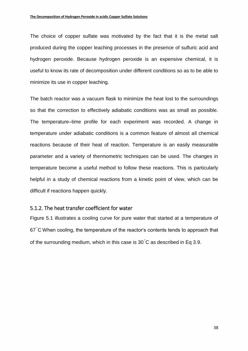
5.1.2. The heat transfer coefficient for water
Figure 5.1 illustrates a cooling curve for pure water that started at a temperature of
67 C. When cooling, the temperature of the reactor‘s contents tends to approach that
of the surrounding medium, which in this case is 30 C as described in Eq 3.9.

The Decomposition of Hydrogen Peroxide in acidic Copper Sulfate Solutions
39
Figure 5.1: Temperature–time profile for the 250ml water contained in a batch
reactor cooling from an initial temperature of 67C which is immersed in a water
batch at a controlled temperature of 30 C.
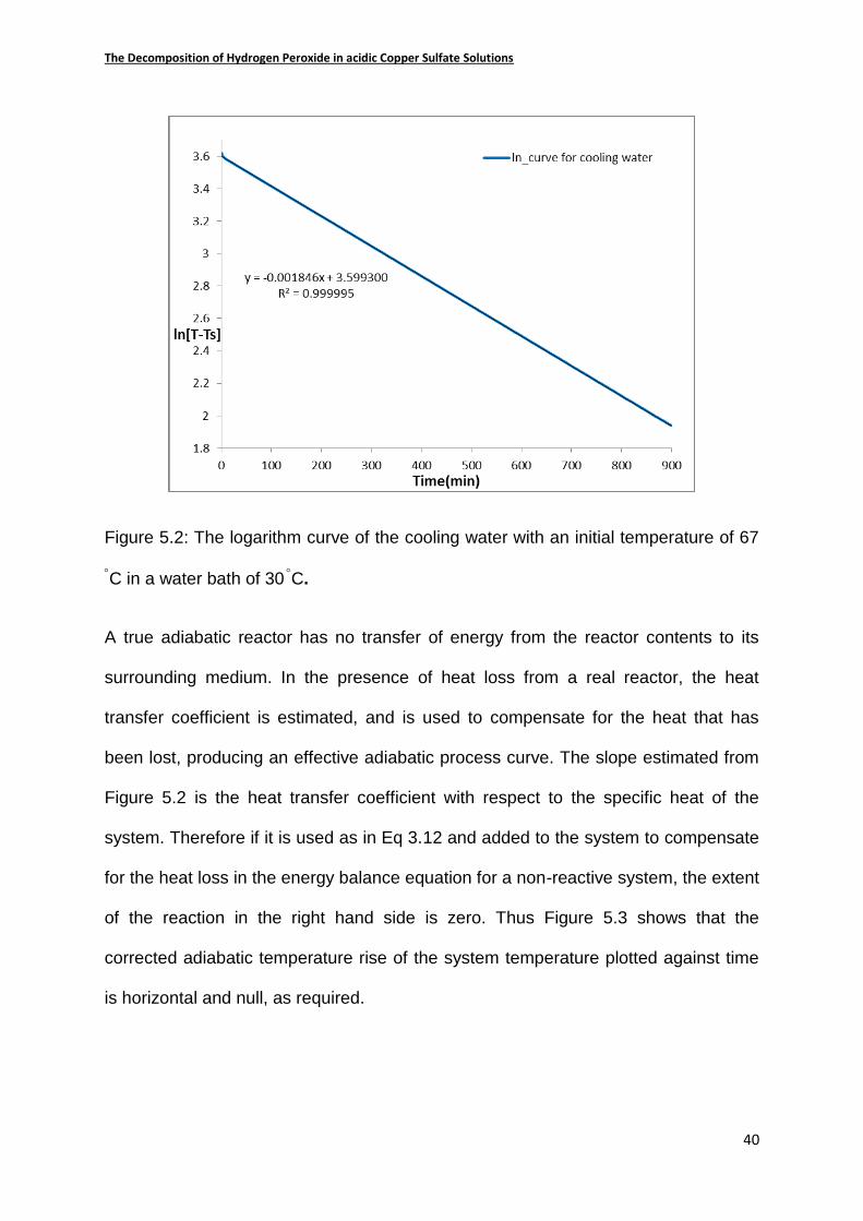
The cooling process of water in this experiment is due to heat transfer only as there
is no reaction taking place. The natural logarithm of the difference between the
temperature of the reactor contents and the water in the bath (Eq 3.12) is plotted
against time in Figure 5.2. In every other result that follows, this plot will be referred
to as “the linear plot”. The linear trend line gives a coefficient of determination (R2) of
0.9999, which is shown to be an excellent fit for this curve. The slope of the linear
curve in Figure 5.2 is estimated from the trend line and found to be -1.846 x 10⁻³ min-
1. This is the value of (UA
MCP) for the non-reactive situation described in Equation
3.12.
The Decomposition of Hydrogen Peroxide in acidic Copper Sulfate Solutions
40
Figure 5.2: The logarithm curve of the cooling water with an initial temperature of 67
C in a water bath of 30 C.
A true adiabatic reactor has no transfer of energy from the reactor contents to its
surrounding medium. In the presence of heat loss from a real reactor, the heat
transfer coefficient is estimated, and is used to compensate for the heat that has
been lost, producing an effective adiabatic process curve. The slope estimated from
Figure 5.2 is the heat transfer coefficient with respect to the specific heat of the
system. Therefore if it is used as in Eq 3.12 and added to the system to compensate
for the heat loss in the energy balance equation for a non-reactive system, the extent
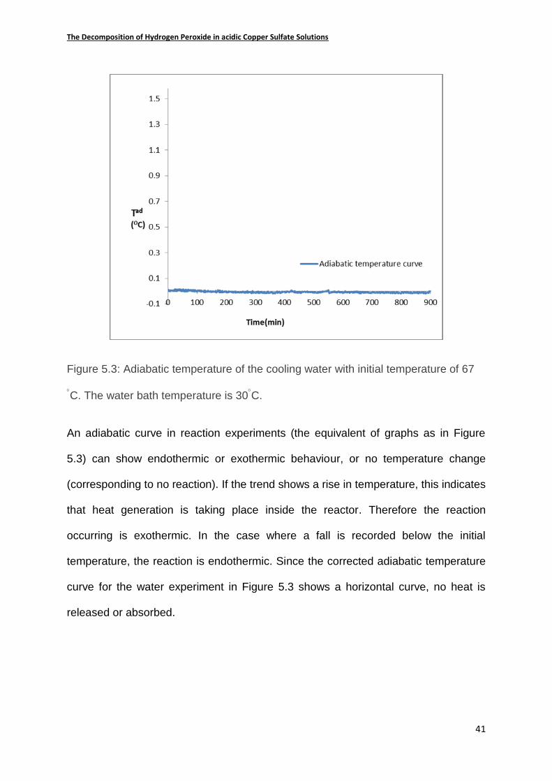
of the reaction in the right hand side is zero. Thus Figure 5.3 shows that the
corrected adiabatic temperature rise of the system temperature plotted against time
is horizontal and null, as required.
The Decomposition of Hydrogen Peroxide in acidic Copper Sulfate Solutions
41
Figure 5.3: Adiabatic temperature of the cooling water with initial temperature of 67
C. The water bath temperature is 30C.
An adiabatic curve in reaction experiments (the equivalent of graphs as in Figure
5.3) can show endothermic or exothermic behaviour, or no temperature change
(corresponding to no reaction). If the trend shows a rise in temperature, this indicates
that heat generation is taking place inside the reactor. Therefore the reaction
occurring is exothermic. In the case where a fall is recorded below the initial
temperature, the reaction is endothermic. Since the corrected adiabatic temperature
curve for the water experiment in Figure 5.3 shows a horizontal curve, no heat is
released or absorbed.
The Decomposition of Hydrogen Peroxide in acidic Copper Sulfate Solutions
42
5.2. The rate of decomposition of hydrogen peroxide
In this section the decomposition of hydrogen peroxide is evaluated as a function of
different initial temperatures. The initial temperature of the reactor contents was
varied from 47C to 67C, while the amounts of hydrogen peroxide injected were
varied between 5ml and 30ml. The mass of copper sulfate used was also varied (i.e.
5g to 20g). All other constituents were kept constant, and the water bath temperature
was controlled at 30C throughout the experiments. The changes in temperature
inside the reactor were recorded.
5.2.1. The effect of temperature
In this set of experiments, 5ml of hydrogen peroxide is injected into a solution of 1M
of sulfuric acid solution and 0.3144M of copper sulfate at different initial
temperatures (47C, 53C, 58C and 67C). Throughout the experimentation, the
reactor’s content was stirred, using a removable magnetic stirrer, at constant speed
to keep the temperature and composition of the solution uniform. A thermocouple
was used as the temperature measuring device.
Figure 5.4 displays the measured temperatures as a function of time. Note that the
concentration of the constituents of the solution was kept constant, and only the
initial temperatures were varied. The effects of the initial temperature on the reacting
solution showed an increment in the heat generated. It is evident that the change in
initial temperature results in the change of the rate of decomposition of hydrogen
peroxide. At the lowest temperature of 47C there is very little temperature rise and
this initial increase gets larger as the initial temperature increases. However, the rise
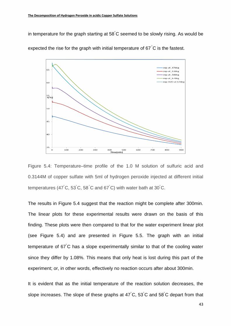
The Decomposition of Hydrogen Peroxide in acidic Copper Sulfate Solutions
43
in temperature for the graph starting at 58C seemed to be slowly rising. As would be
expected the rise for the graph with initial temperature of 67 C is the fastest.
Figure 5.4: Temperature–time profile of the 1.0 M solution of sulfuric acid and
0.3144M of copper sulfate with 5ml of hydrogen peroxide injected at different initial
temperatures (47C, 53C, 58 C and 67C) with water bath at 30C.
The results in Figure 5.4 suggest that the reaction might be complete after 300min.
The linear plots for these experimental results were drawn on the basis of this
finding. These plots were then compared to that for the water experiment linear plot
(see Figure 5.4) and are presented in Figure 5.5. The graph with an initial
temperature of 67C has a slope experimentally similar to that of the cooling water
since they differ by 1.08%. This means that only heat is lost during this part of the
experiment; or, in other words, effectively no reaction occurs after about 300min.
It is evident that as the initial temperature of the reaction solution decreases, the
slope increases. The slope of these graphs at 47C, 53C and 58C depart from that
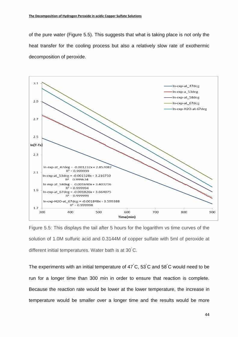
The Decomposition of Hydrogen Peroxide in acidic Copper Sulfate Solutions
44
of the pure water (Figure 5.5). This suggests that what is taking place is not only the
heat transfer for the cooling process but also a relatively slow rate of exothermic
decomposition of peroxide.
Figure 5.5: This displays the tail after 5 hours for the logarithm vs time curves of the
solution of 1.0M sulfuric acid and 0.3144M of copper sulfate with 5ml of peroxide at
different initial temperatures. Water bath is at 30C.
The experiments with an initial temperature of 47C, 53C and 58C would need to be
run for a longer time than 300 min in order to ensure that reaction is complete.
Because the reaction rate would be lower at the lower temperature, the increase in
temperature would be smaller over a longer time and the results would be more
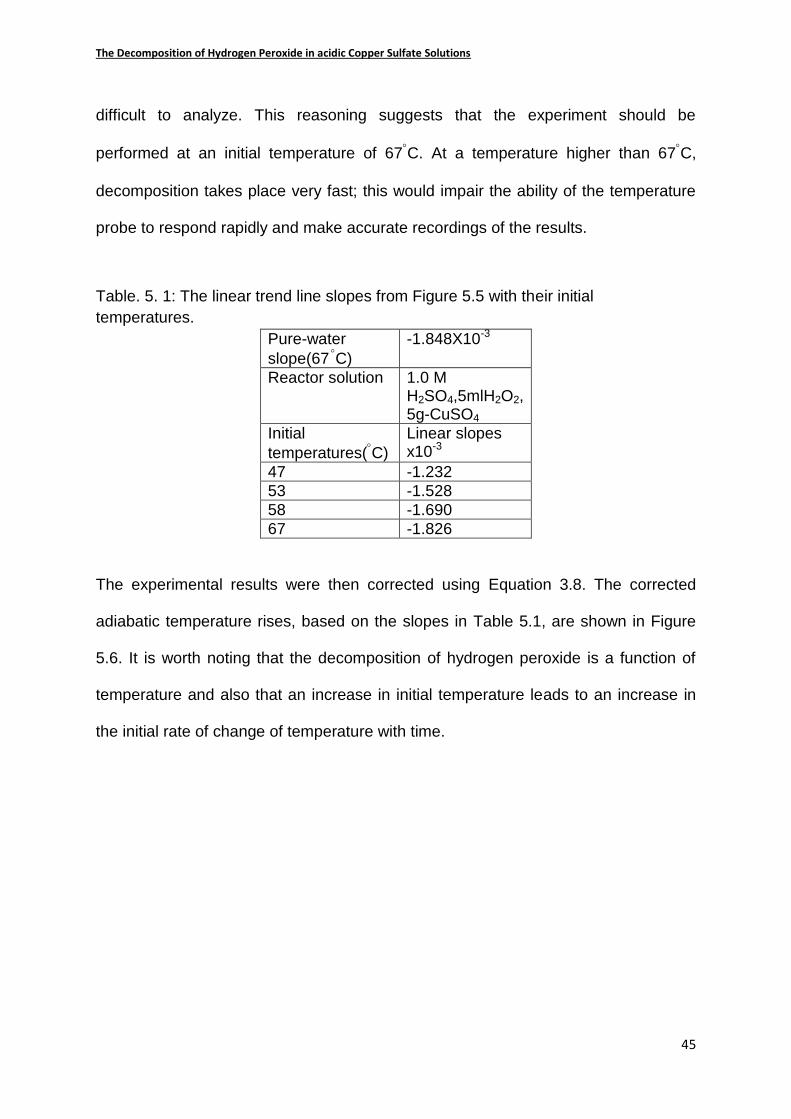
The Decomposition of Hydrogen Peroxide in acidic Copper Sulfate Solutions
45
difficult to analyze. This reasoning suggests that the experiment should be
performed at an initial temperature of 67C. At a temperature higher than 67C,
decomposition takes place very fast; this would impair the ability of the temperature
probe to respond rapidly and make accurate recordings of the results.
Table. 5. 1: The linear trend line slopes from Figure 5.5 with their initial
temperatures.
Pure-water
slope(67 C)
-1.848X10⁻³
Reactor solution 1.0 M H2SO4,5mlH2O2,5g-CuSO4
Initial
temperatures(C)
Linear slopes x10-3
47 -1.232
53 -1.528
58 -1.690
67 -1.826
The experimental results were then corrected using Equation 3.8. The corrected
adiabatic temperature rises, based on the slopes in Table 5.1, are shown in Figure
5.6. It is worth noting that the decomposition of hydrogen peroxide is a function of
temperature and also that an increase in initial temperature leads to an increase in
the initial rate of change of temperature with time.
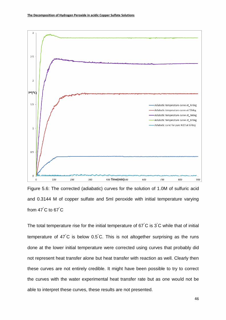
The Decomposition of Hydrogen Peroxide in acidic Copper Sulfate Solutions
46
Figure 5.6: The corrected (adiabatic) curves for the solution of 1.0M of sulfuric acid
and 0.3144 M of copper sulfate and 5ml peroxide with initial temperature varying
from 47C to 67C
The total temperature rise for the initial temperature of 67C is 3C while that of initial
temperature of 47C is below 0.5C. This is not altogether surprising as the runs
done at the lower initial temperature were corrected using curves that probably did
not represent heat transfer alone but heat transfer with reaction as well. Clearly then
these curves are not entirely credible. It might have been possible to try to correct
the curves with the water experimental heat transfer rate but as one would not be
able to interpret these curves, these results are not presented.
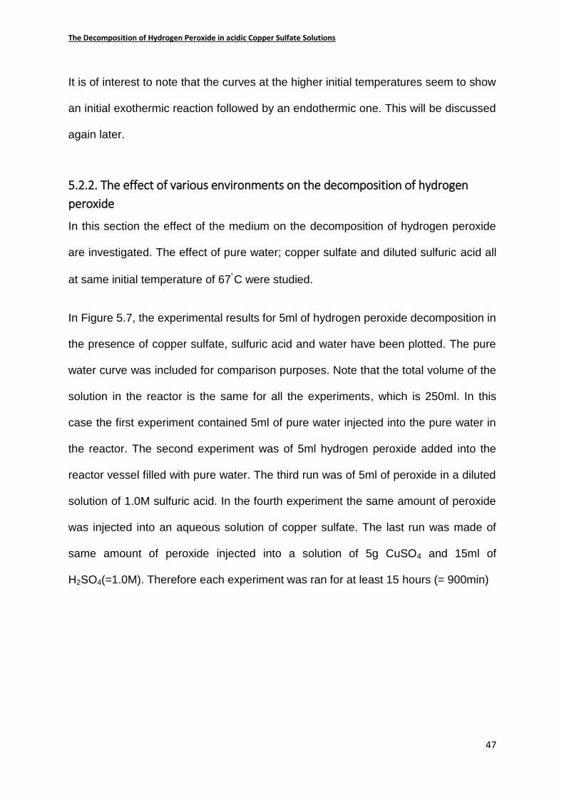
The Decomposition of Hydrogen Peroxide in acidic Copper Sulfate Solutions
47
It is of interest to note that the curves at the higher initial temperatures seem to show
an initial exothermic reaction followed by an endothermic one. This will be discussed
again later.
5.2.2. The effect of various environments on the decomposition of hydrogen
peroxide
In this section the effect of the medium on the decomposition of hydrogen peroxide
are investigated. The effect of pure water; copper sulfate and diluted sulfuric acid all
at same initial temperature of 67C were studied.
In Figure 5.7, the experimental results for 5ml of hydrogen peroxide decomposition in
the presence of copper sulfate, sulfuric acid and water have been plotted. The pure
water curve was included for comparison purposes. Note that the total volume of the
solution in the reactor is the same for all the experiments, which is 250ml. In this
case the first experiment contained 5ml of pure water injected into the pure water in
the reactor. The second experiment was of 5ml hydrogen peroxide added into the
reactor vessel filled with pure water. The third run was of 5ml of peroxide in a diluted
solution of 1.0M sulfuric acid. In the fourth experiment the same amount of peroxide
was injected into an aqueous solution of copper sulfate. The last run was made of
same amount of peroxide injected into a solution of 5g CuSO4 and 15ml of
H2SO4(=1.0M). Therefore each experiment was ran for at least 15 hours (= 900min)
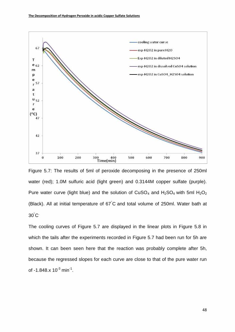
The Decomposition of Hydrogen Peroxide in acidic Copper Sulfate Solutions
48
Figure 5.7: The results of 5ml of peroxide decomposing in the presence of 250ml
water (red); 1.0M sulfuric acid (light green) and 0.3144M copper sulfate (purple).
Pure water curve (light blue) and the solution of CuSO4 and H2SO4 with 5ml H2O2
(Black). All at initial temperature of 67C and total volume of 250ml. Water bath at
30C.
The cooling curves of Figure 5.7 are displayed in the linear plots in Figure 5.8 in
which the tails after the experiments recorded in Figure 5.7 had been run for 5h are
shown. It can been seen here that the reaction was probably complete after 5h,
because the regressed slopes for each curve are close to that of the pure water run
of -1.848.x 10-3 min-1.
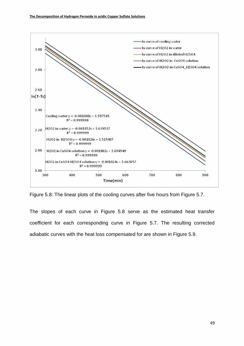
The Decomposition of Hydrogen Peroxide in acidic Copper Sulfate Solutions
49
Figure 5.8: The linear plots of the cooling curves after five hours from Figure 5.7.
The slopes of each curve in Figure 5.8 serve as the estimated heat transfer
coefficient for each corresponding curve in Figure 5.7. The resulting corrected
adiabatic curves with the heat loss compensated for are shown in Figure 5.9.
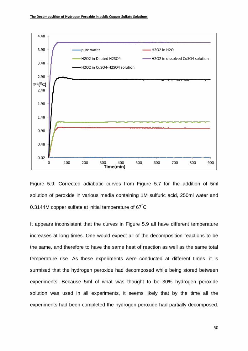
The Decomposition of Hydrogen Peroxide in acidic Copper Sulfate Solutions
50
Figure 5.9: Corrected adiabatic curves from Figure 5.7 for the addition of 5ml
solution of peroxide in various media containing 1M sulfuric acid, 250ml water and
0.3144M copper sulfate at initial temperature of 67C
It appears inconsistent that the curves in Figure 5.9 all have different temperature
increases at long times. One would expect all of the decomposition reactions to be
the same, and therefore to have the same heat of reaction as well as the same total
temperature rise. As these experiments were conducted at different times, it is
surmised that the hydrogen peroxide had decomposed while being stored between
experiments. Because 5ml of what was thought to be 30% hydrogen peroxide
solution was used in all experiments, it seems likely that by the time all the
experiments had been completed the hydrogen peroxide had partially decomposed.
-0.02
0.48
0.98
1.48
1.98
2.48
2.98
3.48
3.98
4.48
0 100 200 300 400 500 600 700 800 900
Tad(OC)
Time(min)
pure water H2O2 in H2O
H2O2 in Diluted H2SO4 H2O2 in dissolved CuSO4 solution
H2O2 in CuSO4-H2SO4 solution
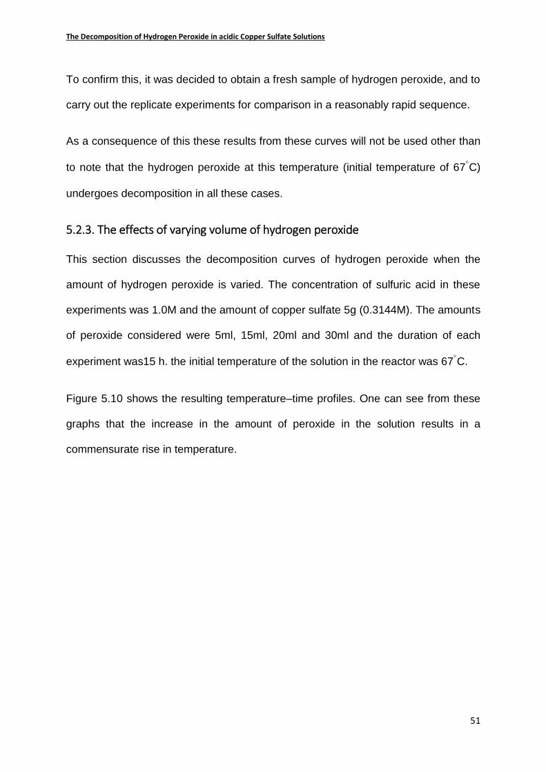
The Decomposition of Hydrogen Peroxide in acidic Copper Sulfate Solutions
51
To confirm this, it was decided to obtain a fresh sample of hydrogen peroxide, and to
carry out the replicate experiments for comparison in a reasonably rapid sequence.
As a consequence of this these results from these curves will not be used other than
to note that the hydrogen peroxide at this temperature (initial temperature of 67C)
undergoes decomposition in all these cases.
5.2.3. The effects of varying volume of hydrogen peroxide
This section discusses the decomposition curves of hydrogen peroxide when the
amount of hydrogen peroxide is varied. The concentration of sulfuric acid in these
experiments was 1.0M and the amount of copper sulfate 5g (0.3144M). The amounts
of peroxide considered were 5ml, 15ml, 20ml and 30ml and the duration of each
experiment was15 h. the initial temperature of the solution in the reactor was 67C.
Figure 5.10 shows the resulting temperature–time profiles. One can see from these
graphs that the increase in the amount of peroxide in the solution results in a
commensurate rise in temperature.
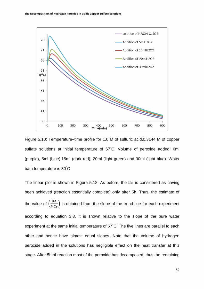
The Decomposition of Hydrogen Peroxide in acidic Copper Sulfate Solutions
52
Figure 5.10: Temperature–time profile for 1.0 M of sulfuric acid,0.3144 M of copper
sulfate solutions at initial temperature of 67C. Volume of peroxide added: 0ml
(purple), 5ml (blue),15ml (dark red), 20ml (light green) and 30ml (light blue). Water
bath temperature is 30C.
The linear plot is shown in Figure 5.12. As before, the tail is considered as having
been achieved (reaction essentially complete) only after 5h. Thus, the estimate of
the value of (UA
MCP) is obtained from the slope of the trend line for each experiment
according to equation 3.8. It is shown relative to the slope of the pure water
experiment at the same initial temperature of 67C. The five lines are parallel to each
other and hence have almost equal slopes. Note that the volume of hydrogen
peroxide added in the solutions has negligible effect on the heat transfer at this
stage. After 5h of reaction most of the peroxide has decomposed, thus the remaining
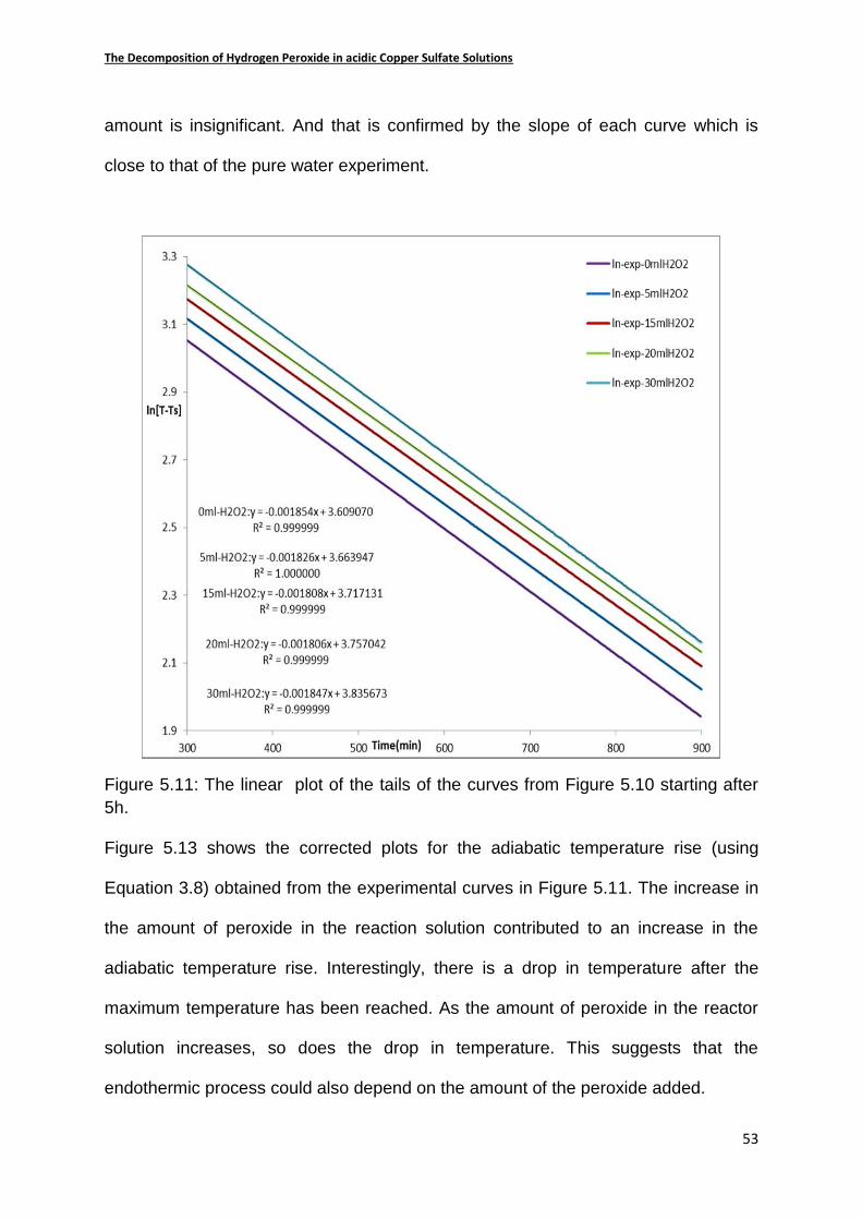
The Decomposition of Hydrogen Peroxide in acidic Copper Sulfate Solutions
53
amount is insignificant. And that is confirmed by the slope of each curve which is
close to that of the pure water experiment.
Figure 5.11: The linear plot of the tails of the curves from Figure 5.10 starting after
5h.
Figure 5.13 shows the corrected plots for the adiabatic temperature rise (using
Equation 3.8) obtained from the experimental curves in Figure 5.11. The increase in
the amount of peroxide in the reaction solution contributed to an increase in the
adiabatic temperature rise. Interestingly, there is a drop in temperature after the
maximum temperature has been reached. As the amount of peroxide in the reactor
solution increases, so does the drop in temperature. This suggests that the
endothermic process could also depend on the amount of the peroxide added.

The Decomposition of Hydrogen Peroxide in acidic Copper Sulfate Solutions
54
Table 5.2 below shows the amount of peroxide added, with the temperature rise to
the maximum, and the subsequent drop for each graph. Each of the curves in Figure
5.12 shows a sharp change in slope at about 200min. This could be attributable to a
slight inaccuracy in the correction to adiabatic temperature, as no allowance was
made for the endothermic reaction. It is also believed that the correction does not
make any significant difference up to this point, and that therefore the results are
credible.
Figure 5.12: The corrected adiabatic curves of the decomposition reaction of
hydrogen peroxide from the results in Figure 5.11.
The change in temperature between the initial and maximum temperature (rise) and
between the maximum and the asymptotic temperature (drop) is shown in Table 5.2,
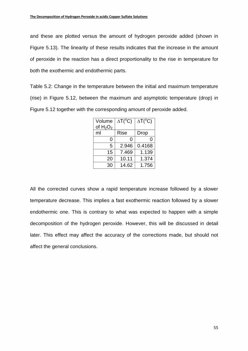
The Decomposition of Hydrogen Peroxide in acidic Copper Sulfate Solutions
55
and these are plotted versus the amount of hydrogen peroxide added (shown in
Figure 5.13). The linearity of these results indicates that the increase in the amount
of peroxide in the reaction has a direct proportionality to the rise in temperature for
both the exothermic and endothermic parts.
Table 5.2: Change in the temperature between the initial and maximum temperature
(rise) in Figure 5.12, between the maximum and asymptotic temperature (drop) in
Figure 5.12 together with the corresponding amount of peroxide added.
Volume of H2O2
∆T(oC) ∆T(oC)
ml Rise Drop
0 0 0
5 2.946 0.4168
15 7.469 1.139
20 10.11 1.374
30 14.62 1.756
All the corrected curves show a rapid temperature increase followed by a slower
temperature decrease. This implies a fast exothermic reaction followed by a slower
endothermic one. This is contrary to what was expected to happen with a simple
decomposition of the hydrogen peroxide. However, this will be discussed in detail
later. This effect may affect the accuracy of the corrections made, but should not
affect the general conclusions.
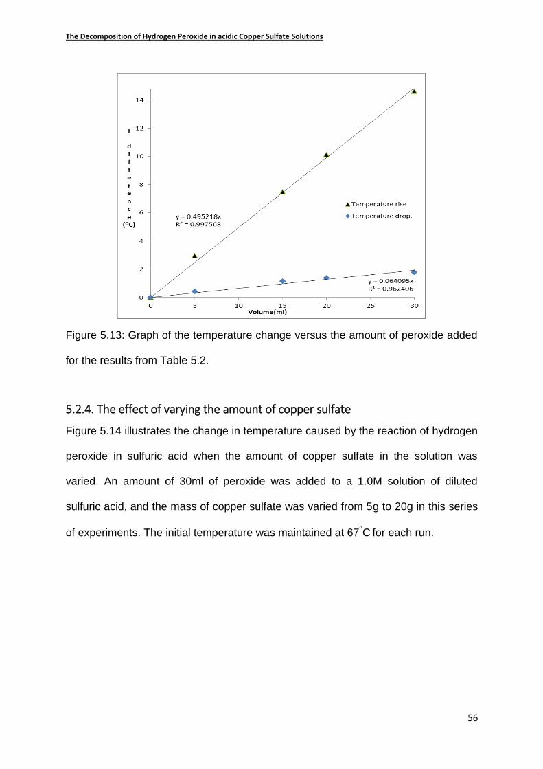
The Decomposition of Hydrogen Peroxide in acidic Copper Sulfate Solutions
56
Figure 5.13: Graph of the temperature change versus the amount of peroxide added
for the results from Table 5.2.
5.2.4. The effect of varying the amount of copper sulfate
Figure 5.14 illustrates the change in temperature caused by the reaction of hydrogen
peroxide in sulfuric acid when the amount of copper sulfate in the solution was
varied. An amount of 30ml of peroxide was added to a 1.0M solution of diluted
sulfuric acid, and the mass of copper sulfate was varied from 5g to 20g in this series
of experiments. The initial temperature was maintained at 67C for each run.
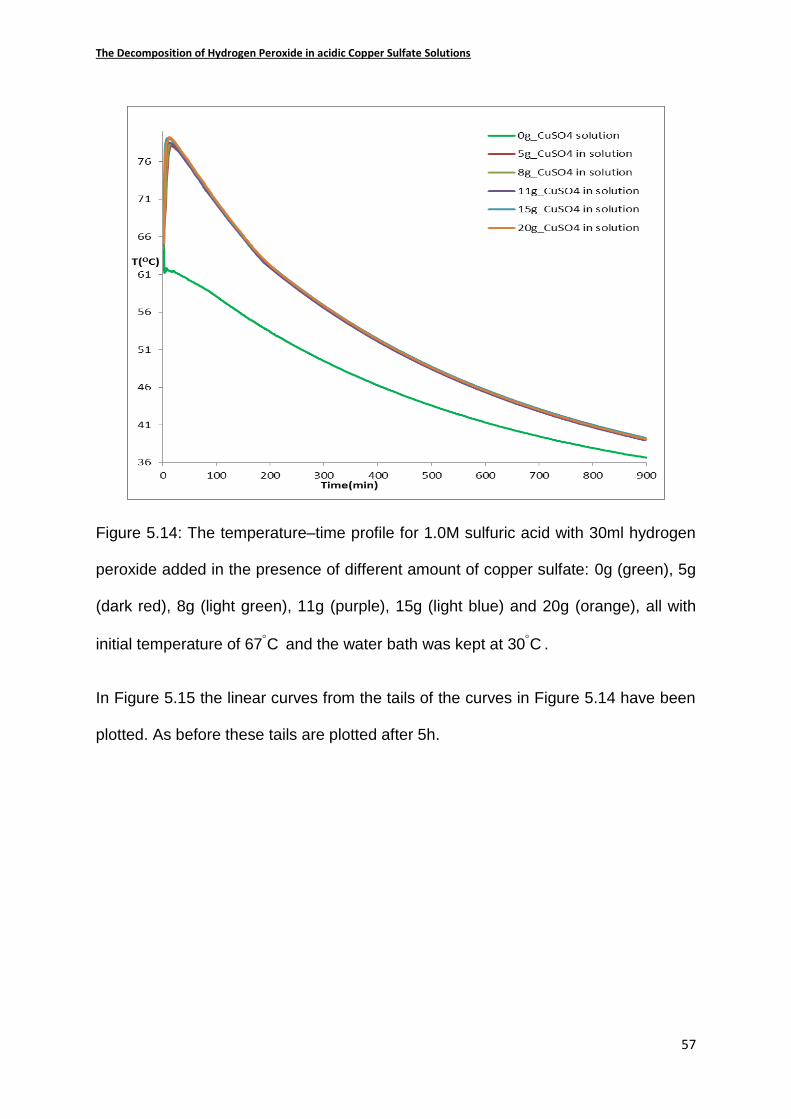
The Decomposition of Hydrogen Peroxide in acidic Copper Sulfate Solutions
57
Figure 5.14: The temperature–time profile for 1.0M sulfuric acid with 30ml hydrogen
peroxide added in the presence of different amount of copper sulfate: 0g (green), 5g
(dark red), 8g (light green), 11g (purple), 15g (light blue) and 20g (orange), all with
initial temperature of 67C and the water bath was kept at 30C .
In Figure 5.15 the linear curves from the tails of the curves in Figure 5.14 have been
plotted. As before these tails are plotted after 5h.
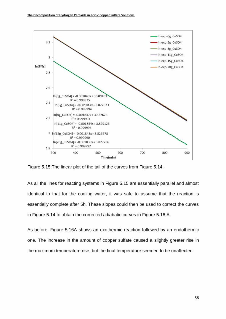
The Decomposition of Hydrogen Peroxide in acidic Copper Sulfate Solutions
58
Figure 5.15:The linear plot of the tail of the curves from Figure 5.14.
As all the lines for reacting systems in Figure 5.15 are essentially parallel and almost
identical to that for the cooling water, it was safe to assume that the reaction is
essentially complete after 5h. These slopes could then be used to correct the curves
in Figure 5.14 to obtain the corrected adiabatic curves in Figure 5.16.A.
As before, Figure 5.16A shows an exothermic reaction followed by an endothermic
one. The increase in the amount of copper sulfate caused a slightly greater rise in
the maximum temperature rise, but the final temperature seemed to be unaffected.
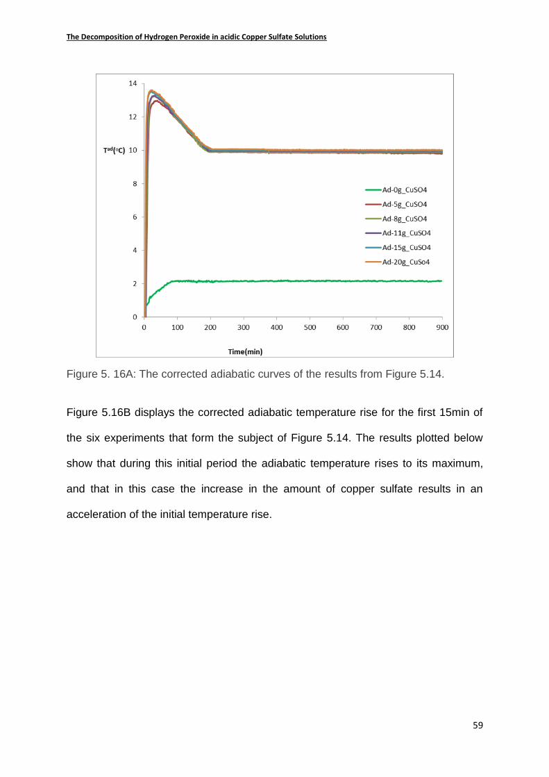
The Decomposition of Hydrogen Peroxide in acidic Copper Sulfate Solutions
59
Figure 5. 16A: The corrected adiabatic curves of the results from Figure 5.14.
Figure 5.16B displays the corrected adiabatic temperature rise for the first 15min of
the six experiments that form the subject of Figure 5.14. The results plotted below
show that during this initial period the adiabatic temperature rises to its maximum,
and that in this case the increase in the amount of copper sulfate results in an
acceleration of the initial temperature rise.
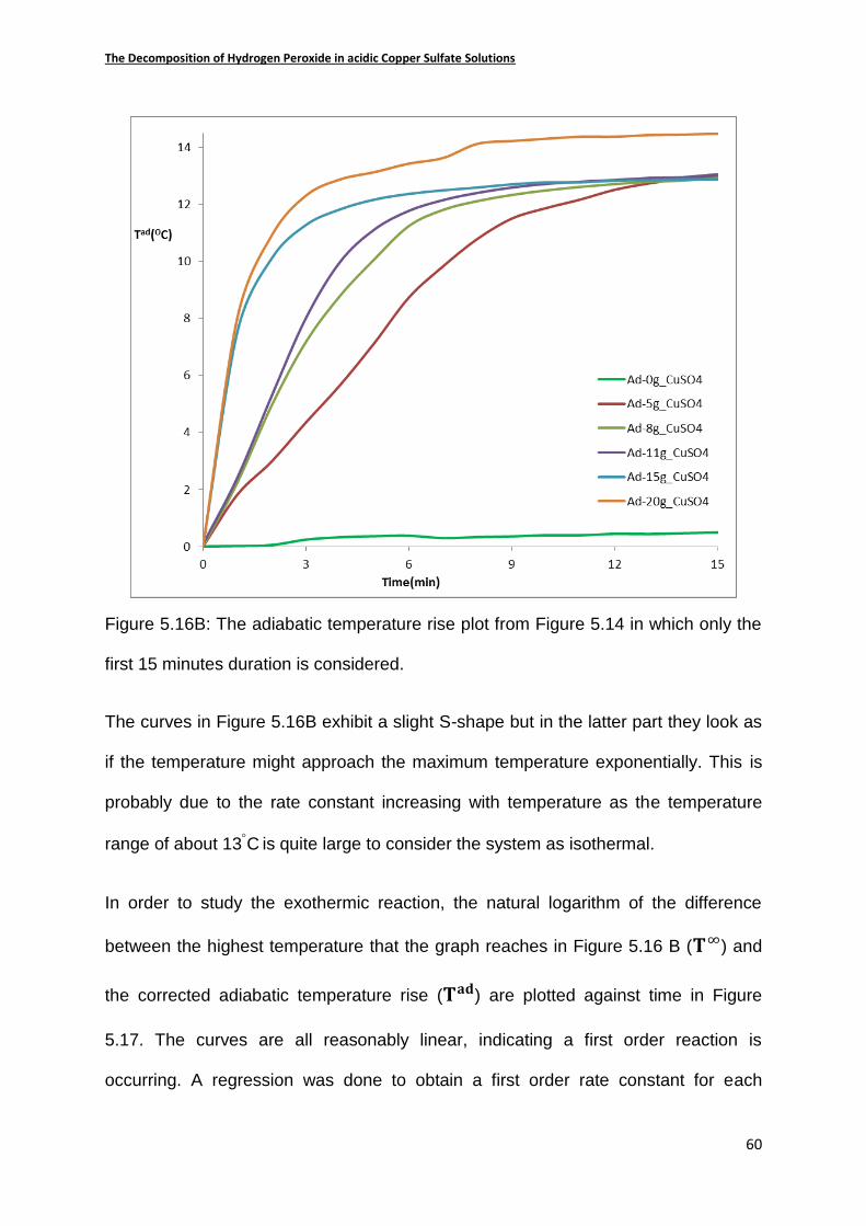
The Decomposition of Hydrogen Peroxide in acidic Copper Sulfate Solutions
60
Figure 5.16B: The adiabatic temperature rise plot from Figure 5.14 in which only the
first 15 minutes duration is considered.
The curves in Figure 5.16B exhibit a slight S-shape but in the latter part they look as
if the temperature might approach the maximum temperature exponentially. This is
probably due to the rate constant increasing with temperature as the temperature
range of about 13C is quite large to consider the system as isothermal.
In order to study the exothermic reaction, the natural logarithm of the difference
between the highest temperature that the graph reaches in Figure 5.16 B (𝐓∞) and
the corrected adiabatic temperature rise (𝐓𝐚𝐝) are plotted against time in Figure
5.17. The curves are all reasonably linear, indicating a first order reaction is
occurring. A regression was done to obtain a first order rate constant for each
The Decomposition of Hydrogen Peroxide in acidic Copper Sulfate Solutions
61
experiment. Equation 5.1 probably describes the exothermic reaction taking place in
this system (Costa, et al. 2006). For the generation of heat which results in a rise in
temperature of the system is probably from this catalytic decomposition of peroxide.
𝐇𝟐𝑶𝟐 → 𝐇𝟐𝐎 +𝟏
𝟐𝑶𝟐 𝟓. 𝟏
5.2.4.1. Effects of copper on reaction constant
It is evident from Figure 5.17 that the greater the amount of copper sulfate, the
greater the first order rate constant for decay will be. The values of these rate
constants with the amount of copper sulfate added are shown in Table 5.3.
It should be noted that doing these plots to get the so-called first order rate constants
is contingent on the fact that the exothermic reaction is essentially complete before
the endothermic reaction starts. These results appear to justify this assumption.

The Decomposition of Hydrogen Peroxide in acidic Copper Sulfate Solutions
62
Figure 5. 17: The 𝐥𝐧(𝐓∞ − 𝐓𝐚𝐝) for the decomposition of hydrogen peroxide with
different amounts of copper sulfate against time. In this case 0g (Orange), 5g (Blue),
8g (Dark red), 11g (Light green), 15g (Purple) and 20g (Green) of copper sulfate is in
solution with 1.0M sulfuric acid and 30ml of peroxide is added. The experiments are
done with an initial temperature of 67 C.
As previously mentioned the slopes of the regression curves in Figure 5.17 provide
the estimated rate constants for first order reaction for each corresponding amount of
copper sulfate. Table 5.3 contains the mass of copper sulfate with the corresponding
estimated rate constants which is plotted in Figure 5.18.

The Decomposition of Hydrogen Peroxide in acidic Copper Sulfate Solutions
63
Table 5.3: The estimated rate constants with the corresponding amount of copper
sulfate added.
Mass(g) of
CuSO4
Estimated rate
constant(k)
0 0.03858
5 0.2659
8 0.3145
11 0.3999
15 0.4331
20 0.4637
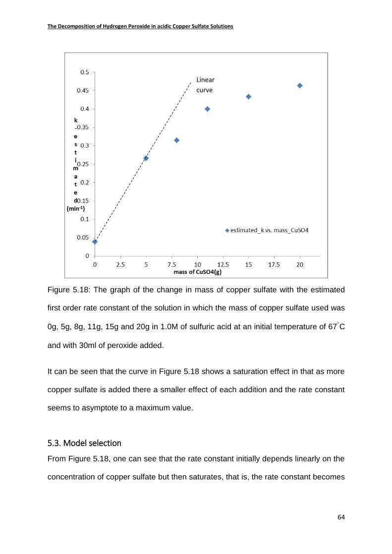
The Decomposition of Hydrogen Peroxide in acidic Copper Sulfate Solutions
64
Figure 5.18: The graph of the change in mass of copper sulfate with the estimated
first order rate constant of the solution in which the mass of copper sulfate used was
0g, 5g, 8g, 11g, 15g and 20g in 1.0M of sulfuric acid at an initial temperature of 67C
and with 30ml of peroxide added.
It can be seen that the curve in Figure 5.18 shows a saturation effect in that as more
copper sulfate is added there a smaller effect of each addition and the rate constant
seems to asymptote to a maximum value.
5.3. Model selection
From Figure 5.18, one can see that the rate constant initially depends linearly on the
concentration of copper sulfate but then saturates, that is, the rate constant becomes
Linear
curve
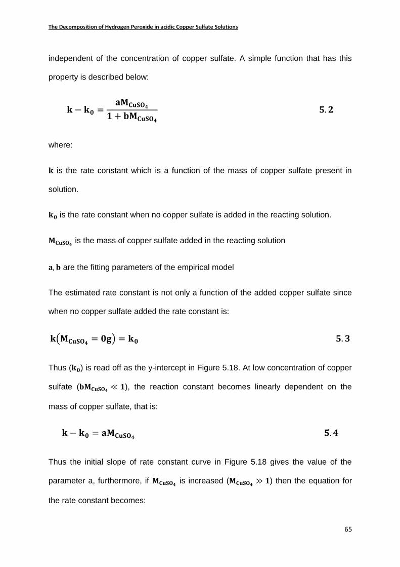
The Decomposition of Hydrogen Peroxide in acidic Copper Sulfate Solutions
65
independent of the concentration of copper sulfate. A simple function that has this
property is described below:
𝐤 − 𝐤𝟎 =𝐚𝐌𝐂𝐮𝐒𝐎𝟒
𝟏 + 𝐛𝐌𝐂𝐮𝐒𝐎𝟒 𝟓. 𝟐
where:
𝐤 is the rate constant which is a function of the mass of copper sulfate present in
solution.
𝐤𝟎 is the rate constant when no copper sulfate is added in the reacting solution.
𝐌𝐂𝐮𝐒𝐎𝟒 is the mass of copper sulfate added in the reacting solution
𝐚, 𝐛 are the fitting parameters of the empirical model
The estimated rate constant is not only a function of the added copper sulfate since
when no copper sulfate added the rate constant is:
𝐤(𝐌𝐂𝐮𝐒𝐎𝟒 = 𝟎𝐠) = 𝐤𝟎 𝟓. 𝟑
Thus (𝐤𝟎) is read off as the y-intercept in Figure 5.18. At low concentration of copper
sulfate (𝐛𝐌𝐂𝐮𝐒𝐎𝟒 ≪ 𝟏), the reaction constant becomes linearly dependent on the
mass of copper sulfate, that is:
𝐤 − 𝐤𝟎 = 𝐚𝐌𝐂𝐮𝐒𝐎𝟒 𝟓. 𝟒
Thus the initial slope of rate constant curve in Figure 5.18 gives the value of the
parameter a, furthermore, if 𝐌𝐂𝐮𝐒𝐎𝟒 is increased (𝐌𝐂𝐮𝐒𝐎𝟒 ≫ 𝟏) then the equation for
the rate constant becomes:
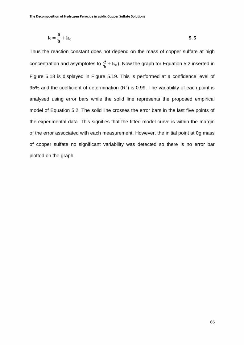
The Decomposition of Hydrogen Peroxide in acidic Copper Sulfate Solutions
66
𝐤 =𝐚
𝐛+ 𝐤𝟎 𝟓. 𝟓
Thus the reaction constant does not depend on the mass of copper sulfate at high
concentration and asymptotes to (𝐚
𝐛+ 𝐤𝟎). Now the graph for Equation 5.2 inserted in
Figure 5.18 is displayed in Figure 5.19. This is performed at a confidence level of
95% and the coefficient of determination (R2) is 0.99. The variability of each point is
analysed using error bars while the solid line represents the proposed empirical
model of Equation 5.2. The solid line crosses the error bars in the last five points of
the experimental data. This signifies that the fitted model curve is within the margin
of the error associated with each measurement. However, the initial point at 0g mass
of copper sulfate no significant variability was detected so there is no error bar
plotted on the graph.

The Decomposition of Hydrogen Peroxide in acidic Copper Sulfate Solutions
67
Figure 5.19: The graph of the amount of copper sulfate against the reaction rate
constants estimated in Figure 5.17 in comparison with the theoretical best fit model
at a confidence level of 95%.
5.3.1. Confidence on the optimized parameters (𝐚, 𝐛) for model The constraints in Equation 5.2 have been optimized at a confidence level of 95%
and are listed in Table 5.4. The value of (𝐚) is estimated to be 0.08333 while (𝐛) is
0.1278.
Table 5.4: Values of optimized parameters in Equation 5.2 computed at a confidence
level of 95%
ko(min-1) 3.858X10⁻²
a(g-1min-1)= 8.333X10⁻² ±0.03158
b(g-1min-1)= 1.278X10⁻² ±0.07643
Confidence level =95%
Coefficient of determination (R2) = 0.99

The Decomposition of Hydrogen Peroxide in acidic Copper Sulfate Solutions
68
In reality the experimental data does not coincide perfectly with the theoretical. The
deviation is due to discrepancies encountered during the performing of the
experimental exercise. The k in Table 5.5 cannot be accurate and precise since it is
derived from experimental findings. Therefore a degree of uncertainty around k has
been allocated based on the allowable error of 5% chosen. This makes the
acceptable region that k can be considered to be enclosed by the maximum and
minimum values. Therefore k+ is the highest acceptable value that k can reach, k-
being the lowest value reachable by k. The ∆k is the amount in which k can increase
or decrease and still be in the accepted region. The region between k+ and k- is
produced by the 5% error which connotes that outside this region the error is higher
than 5%, which is not acceptable. Such evidence in Figure 5.19 is illustrated by the
vertical bars on each coordinate.
Table 5.5: Data for the plot of the mass of copper sulfate against estimated rate
constant (k) showing 95% error bands
Mass(g) of CuSO4 k k+ k- ∆k
0 0.03858 0.04104 0.03612 0.00246
5 0.2659 0.291 0.2408 0.0251
8 0.3145 0.3398 0.2893 0.0253
11 0.3999 0.4287 0.3711 0.0288
15 0.4331 0.4687 0.3976 0.0356
20 0.4637 0.5004 0.427 0.0367
The Endothermic Reaction
Up until now the focus has only been on the exothermic part of the curves in Figure
5.16A. However, it is evident that a substantial endothermic part follows the
The Decomposition of Hydrogen Peroxide in acidic Copper Sulfate Solutions
69
exothermic reaction. When this work was started, it was believed that there was only
a single exothermic reaction taking place, which is seen In Equation 5.1. But, clearly
something more complex is happening.
As this reaction happens when there is no copper sulfate present it is likely to be as
a result of the presence of the sulfuric acid. Nevertheless the investigation on the
endothermic reaction requires more thorough research. This could entail
concentration of the hydroxyl radicals produced, the peroxides and superoxide. This
part of the reaction was not covered in this research. Now it is known that hydrogen
peroxide can react with sulfuric acid to produce Caro’s Acid (Olubambi, Borode and
Ndlovu 2006). Caro's acid (or peroxymonosulfuric acid) is an equilibrium product
obtained by mixing hydrogen peroxide with sulfuric acid.
𝑯𝟐𝑶𝟐 +𝑯𝟐𝑺𝑶𝟒 ↔ 𝑯𝟐𝑺𝑶𝟓 +𝑯𝟐𝑶 𝟓. 𝟔
This is usually thought to occur only in concentrated solutions at low temperature,
but as these reactions at 67C are quite fast, maybe some is produced and nearly
immediately decomposed. If this is the case its decomposition must be endothermic.
This point has not been followed at this stage but could be the focus of more work in
the future.
The Decomposition of Hydrogen Peroxide in acidic Copper Sulfate Solutions
70
Chapter 6
6. Conclusions
In this research the effect of copper sulfate on the decomposition of hydrogen
peroxide was investigated. This was done in the solution of diluted sulfuric acid. An
insulated batch reactor (vacuum flask) was used. The reactor was immersed in a
temperature controlled water bath in order to keep the surrounding temperature of
the reactor constant at 30C. Three variables were considered in doing these
experiments, namely the initial temperature of the reactor contents, the volume of
hydrogen peroxide used, and the amount of copper sulfate added to the process
solution. In each experiment the temperature change of the reactor contents was
monitored as a function of time after the addition of hydrogen peroxide. The
exponential tail of the curves was used to measure the apparent heat loss rate from
the reactor. By measuring the heat transfer rate when only water was present, or
after a long time when it was assumed reaction was essentially complete, the
experimental rate could be corrected to obtain an effective adiabatic curve. These
effective adiabatic curves were then used to interpret the results. In cases when the
apparent heat loss rate did not agree with the one from water it was assumed that
the reaction was too slow and was not essentially complete and so the corrected
results were not that meaningful.
6.1.1. Effect of initial temperature
Four different initial temperatures of the solution, 47C , 53C , 58C and 67C were
used and the same concentration was maintained at 1.0M of sulfuric acid; 5g of
copper sulfate was added and 5ml of injected peroxide. At all the temperatures
except 67C it was observed that the apparent cooling rate was lower than that for
The Decomposition of Hydrogen Peroxide in acidic Copper Sulfate Solutions
71
the pure water, and so it was presumed that the reaction was not complete when the
cooling rate was estimated (after 300 minutes) and hence the lower initial
temperature experiments were not suitable for estimating the kinetics. As a
consequence, all later experiments were done at 67C.
6.1.2. Effects of reaction components on peroxide at 67C
At an initial temperature of 67C , 5ml of hydrogen peroxide was tested in four
different solutions, namely, 250ml of hot water alone; 1.0M of sulfuric acid; 0.3144M
of copper sulfate in a solution of 1.0M of sulfuric acid; and finally with copper sulfate
alone. In this case all the cooling curves were essentially parallel so it was believed
the corrected adiabatic curves could be used. The adiabatic temperature rise for
each of the reaction in the different solutions was very different. This means either
the reaction was not complete when the correction was made or, as was surmised,
because the measurements were done at different times the peroxide had
decomposed while being stored. It was therefore decided that in future fresh
peroxide would be used. Experiments that were to be compared were done as soon
after each other as possible.
6.1.3. Varying the volume of peroxide
The volumes of the hydrogen peroxide added to the reaction solution of 1.0M sulfuric
acid and 5g of copper sulfate were 0ml, 5ml, 15ml, 20ml and 30ml respectively. The
peroxide that was at room temperature was added to the reactor contents at 67C.
All the cooling curves were essentially the same as for the cooling water and
therefore a correction was done to the experimental data. It was very clear from the
experiments that the reaction was not a straightforward exothermic decomposition as
there was both an exothermic followed by an endothermic reaction. It was shown
The Decomposition of Hydrogen Peroxide in acidic Copper Sulfate Solutions
72
that the maximum adiabatic temperature rise was proportional to the amount of
peroxide added, so was the subsequent adiabatic temperature drop. It was therefore
concluded that there are at least two reactions occurring, both a function of the
amount of peroxide present.
6.1.4. The role of copper sulfate in the reaction
Different amounts of copper sulfate were used, namely 0g, 5g, 8g, 11g, 15g and 20g,
which were added to a 1.0M of diluted sulfuric acid with an initial temperature of 67C
. Then 30ml of hydrogen peroxide which was at room temperature was injected into
the solution at 67C initial temperature. It was observed that the change in the
amount of copper sulfate affected the rate of decomposition of peroxide since the
higher the amount of copper sulfate the faster the reaction occurred. It is worth
noting that the change in the amount of copper sulfate had no effect on the rate of
the side reaction.
6.1.5. Rate determination
This study has shown that an increase in the amount of copper sulfate in the reacting
solution increases the rate of decomposition of peroxide. It was further found that for
each experiment the decomposition of peroxide followed a first order rate. When the
first order rate constants were plotted against the amount of copper sulfate present,
the constant increased steeply initially as the copper catalyzes the peroxide but
tailed off as the amount of copper sulfate increased. A simple rate expression that
showed a saturation effect was chosen with two constants. The constants were
estimated and the model was shown to give a good fit to the experimental results.
The Decomposition of Hydrogen Peroxide in acidic Copper Sulfate Solutions
73
As the endothermic part was unaffected by the presence of copper it was not further
analyzed. It was suggested that the decomposition of the hydrogen peroxide was not
a simple process, as it was possible that Caro’s acid was formed, and what we saw
was the decomposition of this as well as of the hydrogen peroxide directly.
6.2. Overall conclusion
The effect of copper sulfate on the kinetics of the decomposition of hydrogen
peroxide was investigated and a model elucidating the effect of the amount of copper
sulfate on the decomposition of peroxide was proposed. The primary decomposition
of peroxide followed a first order rate law as reported in the literature (Croiset, Rice
and Hanush 1997). As would be expected, it was also found that in an adiabatic
reactor the maximum temperature rise of the reacting solution was found to be
proportional to the amount of hydrogen peroxide added. Furthermore it was shown
that copper sulfate served as a catalyst for the decomposition of hydrogen peroxide
in a sulfuric acid solution (Perez-Benito 2004). The decomposition was also shown
to contain an exothermic as well as an endothermic part and a possible explanation
for this was proposed.
Because the copper in solution catalyses the decomposition of the hydrogen
peroxide it would be desirable to keep the copper in industrial leaching solutions as
low as possible. Therefore one would like to continuously remove the copper in
solution during the leaching process. This could for instance be done by the addition
of solvent extraction and electro-winning units in a recycle system with the leaching
unit.
The Decomposition of Hydrogen Peroxide in acidic Copper Sulfate Solutions
74
Solvent extraction provides high concentrations of copper ions (Cu2+) in a solution
using extractants such as aldoximes and ketoximes (Beltran 2009). The solution
with the high concentration of copper is then taken for further purification of copper
in an electro-winning unit while the stream with the lower copper concentration is
returned to the leaching unit for further processing. Thus the amount of peroxide
used in copper leaching solution could be minimized.
The Decomposition of Hydrogen Peroxide in acidic Copper Sulfate Solutions
75
7. References
Haiyu, Y., Liu, J. & Yang, J. 2011, “Leaching Copper from Shredded Particles of
Waste Printed Circuit Boards”, Journal of Hazardous Materials,vol.187,pp. 393-400.
Li, J. & Sheng, G. 2008, “The Research of Copper Leaching from the Waste
Computer Mainboards,” Institute of Electrical and Electronics Engineers, pp.4662-
4666.
Strukul, G. 1992, Catalytic oxidations with hydrogen peroxide as oxidant, Kluwer
academic publishers, AH Dordrecht, Netherlands
Jones, C.W.,1999. Applications of hydrogen peroxide and derivatives. The Royal
Society of Chemistry,Thomas Graham House, Cambridge, UK
Lunsford, J. H. 2003, “The direct formation of H2O2 from H2 and O2 over palladium
catalysts.” Journal of Catalysis, vol.216, pp 455-460.
Solsona, B. E., Edwards, K. J., Landon, P., Carley, A. F., Herzing, A., Kiely, C. J.,
Hutchings, G. J., 2006, “Direct synthesis of hydrogen peroxide from hydrogen and
oxygen using Al2O3 supported AU-Pd catalysts”, American Chemical Society, vol. 18,
no. 11, pp. 2689-2695.
Yildiz, M., & Akin, A. N., 2007, “Direct Formation of H2O2 from H2 and O2”, Turk J
Chem, vol. 31,pp. 479–486.
Abdollahi, M., & Hosseini, A., 2014, “Hydrogen peroxide”, Elsevier inc., vol. 2, pp.
966-970.
Beeman, L A., & Reichert, J. S., 1953, “The Bleaching of pulp”, TAPPI Monography
Series No. 10, New York, Chapter XII.
The Decomposition of Hydrogen Peroxide in acidic Copper Sulfate Solutions
76
Salem, I. A., El-Maazawi, M., Zaki, B. M., 2000, “Kinetics and mechanisms of
decomposition of hydrogen peroxide in presence of metal complexes”, John Wiley &
Sons, Inc, pp. 643-666.
Schmidt, J.T., Ahmad, M., Teel, A.L., Watts, R.J., 2011, “Hydrogen peroxide
stabilization in one-dimensional flow columns,” Journal of Contaminant Hydrology,
vol. 126, pp.1-7.
Buxton, G. V., Greenstock, C.L., Helman, W.P., Ross, A.B., 1988, “Critical review of
rate constant for reactions of hydrated electrons, hydrogen atom and hydroxyl
radicals (OH./O.-) in aqueous solution”, J. Phys. Chem. Ref. Data, vol.17, no. 2, pp.
1-21.
Haag, W. R., & Yao, C.C.D., (1992), “Rate Constants for Reaction of Hydroxyl
Radicals with Several Drinking Water Contaminants”, Environmental Science and
Technology, vol.26, pp.1005–1013.
Watts, R.J., and Teel, A L., 2006, “Treatment of Contaminated Soils and
Groundwater Using ISCO”, Pract. Period. Hazard. Tox. Radioact. Waste
Management, vol. 10, pp.2-9.
Chang, M.W., Chung, C. C., Chern, J. M., Chen. T. S., 2009, “Dye decomposition
kinetics by UV/H2O2: Initial rate analysis by effective kinetic modeling methodology”,
Chemical Engineering Science, Vol.65, pp. 135-140.
Croiset, E., Rice, S.F. & Hanush, R.G., 1997, “Hydrogen peroxide decomposition in
supercritical water”, AIChE Journal, Vol.43, no. 9, pp.3243-2352.

The Decomposition of Hydrogen Peroxide in acidic Copper Sulfate Solutions
77
Oishi, T., Koyama, K., Alam, S., Tanaka, M., & Lee, J.C., (2007) “Recovery of High
Purity Copper Cathode from Printed Circuit Boards using Ammoniacal Sulfate or
Chloride Solutions”, Hydrometallurgy, vol. 89, pp. 82-88.
Olubambi, P.A., & Potgieter, J H., 2009, “Investigation on the Mechanism of Sulfuric
Acid Leaching of Chalcopyrite in the Presence of Hydrogen Peroxide”, Mineral
Processing and Extractive Metallurgy Review, vol. 30, pp.326-345.
Stanley, R. W., Subramanian, N.K., 1977,” Recovering Copper from Concentrates
with Insoluble Sulfate Forming Leach.”, United States of America Patent 4, 039,406.
Frankiewicz, T C., & Lueders, R. E., 1979,”Copper Leaching Employing Nitrogen
Dioxide as Oxidant”, United States of America Patent 4,132,758.
Ekinci, Z., Colak, S., Cakici, A., and Sarac, H., 1998, “Leaching Kinetics of Sphalerite
with Pyrite in Chlorine Saturated Water”, Minerals Engineering, vol. 11, pp.279-283.
Prasad, S, & Pandey, B.D., 1998, “Alternative Process for Treatment of
Chalcopyrite-a Review”, Minerals Engineering, vol. 11, pp. 763-781.
Copur, M., 2001, “Solubility of Concentrate Containing Pyrite and Chalcopyrite in
HNO3 Solutions”, Chemical and Biochemical Engineering Quaterly, vol. 15 pp.181-
184.
Copur, M., 2002, “An Optimization Study of Dissolution of Zn and Cu in ZnS
Concentrate with HNO3 Solutions” Chemical and Biochemical Engineering Quaterly,
vol. 16, pp. 191-197.
Biswas, A K, & Davenport W G., 1980, Extractive Metallurgy of Copper, Oxford,
Pergamon Press, pp.263-269.

The Decomposition of Hydrogen Peroxide in acidic Copper Sulfate Solutions
78
Antonijevic, M.M., & Bogdanovic, G.D., 2004, “Investigation of the Leaching of
Chalcopyritic ore in Acidic Solutions”, Hydrometallurgy, vol. 73, pp. 245-256.
Olubambi, P. A., Borode, J. O., Ndlovu, S., 2006, Sulfuric acid leaching of zinc and
Copper from Nigerian Complex Sulfide Ore in the presence of hydrogen peroxide,
The Journal of the Southern African Institute of Mining and Metallurgy, vol. 106,
pp.765-770.
Jiang, T., Yang, Y., Zhang, B., & Huang, Z., 2002, “Kinetics of Silver Leaching from
Manganese-Silver Associated Ores in Sulfuric Acid Solution in the Presence of
Hydrogen Peroxide”, Metallurgical and Materials Transactions, vol. 33B, pp. 813-
816.
Antonijevic, M. M., Dimitrijevic, M., & Jankovic, Z., 1997, “Leaching of Pyrite with
Hydrogen Peroxide in Sulfuric Acid”, Hydrometallurgy, vol. 46, pp. 71-83.
Adebayo, A O, Ipinmoroti, K.O., & Ajayi, O.O., 2003, “Dissolution Kinetics of
Chalcopyrite with Hydrogen Peroxide in Sulfuric acid Medium”, Chemical and
Biochemical Engineering, vol. 17, pp. 213-218.
Grant, R. C., S J Harwood, S.J., Wells, R.D., 1968, “Catalytic Decomposition of
Hydrogen Peroxide by Copper Chelates and Mixed Ligand Complexes of Histamine
in the Presence of Phosphate Buffer in the Neutral pH Region”, Journal of the
American Chemical Society, vol. 90, no. 16, pp. 4476-4478.
Sigel, H., Flierl, C., & Griesser, R.,1969, “On the Kinetics and Mechanism of the
Decomposition of Hydrogen Peroxide ,Catalyzed by the Cu2+-2,2'-Bipyridyl
Complex.”, Journal of the American Chemical Society, vol. 91, no. 5, pp.1061-1064.
The Decomposition of Hydrogen Peroxide in acidic Copper Sulfate Solutions
79
Erlenmeyer, H., Flierl, C., & Sigel, H.,1969, “On the Kinetics and Mechanism of the
Reactions of Hydrogen Peroxide with Hydrazine or Hydroxylamine, Catalyzed by
Cu2+ and by the Cu2+-2,2'-Bipyridyl Complex”, Journal of the American Chemical
Society, vol. 91, no. 5, pp.1065-1071.
Onuchukwu, A.I., 1984, “Kinetics of the Decomposition of Hydrogen Peroxide
Catalyzed by Copper and Nickel Ferrites”, Journal of Chemical Society, vol. 80,
pp.1447-1456.
Perez-Benito, J.F., 2001, “Copper (II)-Catalyzed Decomposition of Hydrogen
Peroxide: Catalyst Activation by Halides Ions”, Monatshefte fuÈ r Chemie, vol. 132,
pp. 1477-1492.
Haber, F., & Weiss, J., 1934, “The Catalytic Decomposition of Hydrogen Peroxide by
Iron Salt”, The Royal Society, vol. 147, no. 861, pp.332-351.
Kanungo, S B., Parida, K. M., and Sant, B.R., 1981, “Studies on MnO2-III. The
Kinetics and the Mechanism for the Catalytic Decomposition of H2O2 over Different
Crystalline Modifications of MnO2”, Pergamon Press Ltd, vol. 26, no. 8, pp. 1157-
1167.
Borrull, F, & Cerda, V., 1987, “Copper (II) Determination by Means of a
Thermometric Method Based on its Catalytic Effect on the Hydrazine-Hydrogen
Peroxide Reaction”, Elsevier Science Publishers, vol. 112, pp.335-340.
Choudhary, V.R., & Gaikwad, A G., 2003, “Kinetics of Hydrogen Peroxide
Decomposition in Aqueous Sulfuric Acid over Palladium/Carbon: Effect of Acid
Concentration.”, Akadémiai Kiadó, Budapest and Kluwer Academic Publisher,
Dordrecht, vol. 80, no. 1, pp. 27-32.

The Decomposition of Hydrogen Peroxide in acidic Copper Sulfate Solutions
80
Schmidt, L.D., 1998, The engineering of chemical reactions, Oxford University Press,
Inc. New York
Hartridge, H. & Roughton, F. J. W., 1924, Improvement in the apparatus for
measuring the velocity of very rapid chemical reactions, mathematical proceedings
of the Cambridge philosophical society,vol. 22, no. 03,pp. 426-431.
La Mer, V.K., & Read, C.L., 1930, “Rapid Reactions. The Velocity and Heat Effects
involved in the Neutralization of Sodium Dichromate by Sodium Hydroxide”vol. 52
no. 631, pp.3098-3111.
Dyne, S. R, Glasser, D., & King, R. P., 1967. “Automatically Controlled Adiabatic
Reactor for Reaction Rate Studies”, AIP Publishing, vol. 38, no. 209, pp.209-214.
Glasser, D., & Williams, D. F., 1971, “The Study of Liquid-Phase Kinetics using
Temperature as a Measured Variable”, Industrial Engineering Chemistry, vol. 10, no.
3, pp. 516-519.
Scott, P. D., Glasser, D., & Nicol, M.J., 1975, “Thermal Determination of the Kinetics
of the Iron (III)-Tin (II) Redox Reaction in Chloride Solution”, National Institute of
Metallurgy, pp.1413-1421.
Fogler, S.H., 1999, Elements of Chemical Reaction Engineering, Prentice-Hall New
Jersey,
Shatynski, J.J., & Hanesian, D., 1993. “Adiabatic Kinetic Studies of the
Cytidine/Acetic Anhydride Reaction by Utilizing Temperature versus Time Data,”
American Chemical Society, vol. 32, no. 4, pp. 594-599
The Decomposition of Hydrogen Peroxide in acidic Copper Sulfate Solutions
81
Khandpur, R. S., 2005, Printed Circuits Boards: Design, Fabrication, Assembly and
Testing. Tata McGraw-Hill, New Delhi.
Wang, T.P., 1990, “Thermocouple Materials”, The Material Information Society, vol.
2, pp. 88-107.
Katubilwa, F.M., 2012, “Effects of pool volume on wet milling efficiency”, PhD Thesis,
University of the Witwatersrand, Johannesburg
Palm, W.J., 2001, Introduction to Matlab 6 for Engineers, McGraw-Hill, Boston, USA.
Motulsky, H.J., Christopoulos, A., 2003, Fitting models to biological data using linear
and nonlinear regression: A practical guide to curve fitting. GraphPad Software Inc.,
San Diego, www.graphpad.com
Costa, R.C.C., Lelis, M,F.F., Oliveira, L.C.A., Fabris, J.D., Ardisson, J.D.,Rios,
R.R.V.A,Silva, C.N., Lago, R.M., 2006, Novel active heterogeneous Fenton system
based on Fe3-xMxO4 (Fe, Co, Mn, Ni): The role of M2+ species on the reactivity
towards H2O2 reactions. Journal of Hazardous Materials, vol. 129, pp.171-178
Perez-Benito, J.F., 2004,”Reaction pathways in the decomposition of hydrogen
peroxide catalyzed by copper (II)”, Journal of Inorganic Biochemistry, vol. 98, pp.
430–438.
Beltran, M. S.,2009, Recovery of Copper from Electronic Waste, MSc. Thesis,
Chalmers University of Technology, Sweden.