Embed Size (px)
Citation preview

The Deformation Theory of a
Birationally Commutative Surface of
Gelfand-Kirillov Dimension 4
Chris Campbell
Supervisor:
Dr. Susan J. Sierra
Doctor of Philosophy
The University of Edinburgh
2016

ii

The Deformation Theory of a Birationally
Commutative Surface of Gelfand-Kirillov
Dimension 4
Doctoral Dissertation
Chris Campbell
School of MathematicsThe University of Edinburgh
Chris CampbellE-mail: [email protected]
Supervisor: Susan J. SierraE-mail: [email protected]
Examiners:Internal: David JordanExternal: Ulrich Krahmer
School of MathematicsThe University of EdinburghJames Clerk Maxwell BuildingThe King’s BuildingsPeter Guthrie Tait RoadEdinburgh, EH9 3FDUnited Kingdom
©2016 Chris CampbellDoctoral dissertationInitial Submission: 31/05/16Final Submission:Typeset in LATEX

ii

Declaration
I declare that this thesis was composed by myself and that the work contained therein
is my own, except where explicitly stated otherwise. This work has not been submitted
for any other degree or professional qualification.
Edinburgh, July 23, 2016
Place, DateChris Campbell
iii

iv

Lay Abstract
In the pure mathematical field of noncommutative algebra we are interested in under-
standing systems of numbers where the rules that are true for the counting numbers
fail to hold. In particular, we examine abstract number systems where the order in
which you multiply can effect the final result. For example, although in the counting
numbers 3 × 6 = 6 × 3, there are more exotic mathematical settings in which this
equation fails to hold. We call these exotic number systems rings. One of the main
aims of noncommutative algebra is to classify all of the possible rings.
Unfortunately, this goal is currently unattainable. Indeed, this question of classifi-
cation is so hard that we do not even know what kinds of rings could possibly exist, let
alone how to categorise them. For this reason generating new examples of rings allows
us to test our preconceptions of what must or must not be true about them.
One method for generating new examples of rings is to ‘deform’ rings that are
already well understood. For example, the ring of polynomials is made up of elements
like xy + 1 and x2 + 1. In this ring, xy = yx is a rule that always holds. One can ask
however what happens if instead the rule was xy = 2yx. Amazingly, this simple change
to the rule has connections as far afield as quantum mechanics in physics.
In this thesis, we approach a well understood ring and deform it using a method
similar to the above. In our case we adopt a recipe for using symmetries of objects like
the sphere to determine deformations of this ring. In order to do so we develop new
ideas in one large class of rings of interest across mathematics. We then describe how
to apply these ideas in the specific case of this well understood ring.
v

vi
Abstract
Let K be the field of complex numbers. In this thesis we construct new examples ofnoncommutative surfaces of GK-dimension 4 using the language of formal and infinites-imal deformations as introduced by Gerstenhaber. Our approach is to find families ofdeformations of a certain well known GK-dimension 4 birationally commutative surfacedefined by Zhang and Smith in unpublished work cited in [YZ06], which we call A.
Let B∗ and K∗ be respectively the bar and Koszul complexes of a PBW algebraC = K〈V 〉
(R) . We construct a graph whose vertices are elements of the free algebra K〈V 〉and edges are relations in R. We define a map m2 : B2 → K2 that extends to achain map m∗ : B∗ → K∗. This map allows the Gerstenhaber bracket structure to betransferred from the bar complex to the Koszul complex. In particular, m2 provides amechanism for algorithmically determining the set of infinitesimal deformations withvanishing primary obstruction.
Using the computer algebra package ‘Sage’ [Dev15] and a Python package developedby the author [Cam], we calculate the degree 2 component of the second Hochschildcohomology of A. Furthermore, using the map m2 we describe the variety U ⊆ HH2
2(A)of infinitesimal deformations with vanishing primary obstruction. We further show thatU decomposes as a union of 3 irreducible subvarieties Vg, Vq and Vu.
More generally, let C be a Koszul algebra with relations R, and let E be a local-isation of C at some (left and right) Ore set. Since R is homogeneous in degree two,there is an embedding R ↪→ C⊗C and in the following we identify R with its (nonzero)image under this map. We construct an injective linear map Λ : HH2(C) → HH2(E)and prove that if f ∈ HH2(E) satisfies f(R) ⊆ C then f ∈ Im(Λ). In this way wedescribe a relationship between infinitesimal deformations of C with those of E.
Rogalski and Sierra [RS12] have previously examined a family of deformations ofA arising from automorphism of the surface P1 × P1. By applying our understandingof the map Λ we show that these deformations correspond to the variety of infinites-imal deformations Vg. Furthermore, we show that deformations defined similarly byautomorphisms of other minimal rational surfaces also correspond to infinitesimal de-formations lying in Vg.
We introduce a new family of deformations of A, which we call Aq. We show thatelements of this family have families of deformations arising from certain quantumanalogues of geometric automorphisms of minimal rational surfaces, as defined by Alevand Dumas [AD95]. Furthermore, we show that after taking the semi-classical limitq → 1 we obtain a family of deformations of A whose infinitesimal deformation lies inVq.
Finally, we apply a heuristic search method in the space of Hochschild 2-cocycles ofA. This search yields another new family of deformations of A. We show that elementsof this family are non-noetherian PBW noncommutative surfaces with GK-dimension4. We further show that elements of this family can have as function skew field thedivision ring of the quantum plane Kq(u, v), the division ring of the first Weyl algebraD1(K) or the commutative field K(u, v).
vii

viii
Acknowledgements
First and foremost I would like to thank my supervisor Sue Sierra for many hours of
guidance and conversation, without which this thesis would never have been possible. I
would also like to extend this thanks to the Mathematics Department of the University
of Edinburgh more generally for being such a welcoming and exciting place to learn
and research mathematics.
I have had helpful conversations and classes with so many mathematicians over the
past few years that it is hard to single any out. However special thanks to the following
people: Iain Gordon, David Jordan, Adrien Brochier, Cris Negron, Uli Kraehmer, Joe
Karmazyn, Noah White, Simon Crawford, Sian Fryer, Kevin McGerty, Ivan Cheltsov,
Andrew Ranicki and Igor Krylov.
Thanks also to my family who have been nothing but encouraging and provided
much needed sanctuary in times of stress. Finally I would like to thank my wife, Misa,
for providing me with unfailing love and support. Without her I would never have
made it through.
ix

x
Contents
Contents xi
1 Introduction 1
1.1 Motivation . . . . . . . . . . . . . . . . . . . . . . . . . . . . . . . . . . 1
1.2 Summary of Approach . . . . . . . . . . . . . . . . . . . . . . . . . . . . 2
1.3 Summary of General Results . . . . . . . . . . . . . . . . . . . . . . . . 5
1.4 The Deformation Theory of A . . . . . . . . . . . . . . . . . . . . . . . . 6
1.5 Further Work . . . . . . . . . . . . . . . . . . . . . . . . . . . . . . . . . 11
2 Background 13
2.1 Koszul Algebras . . . . . . . . . . . . . . . . . . . . . . . . . . . . . . . 13
2.2 The Algebra A . . . . . . . . . . . . . . . . . . . . . . . . . . . . . . . . 17
2.3 Deformation Theory . . . . . . . . . . . . . . . . . . . . . . . . . . . . . 21
3 The Second Hochschild Cohomology Space for Two Algebras of In-
terest 29
3.1 Introduction . . . . . . . . . . . . . . . . . . . . . . . . . . . . . . . . . . 29
3.2 Calculations of Hochschild Cohomology Spaces . . . . . . . . . . . . . . 30
3.3 The Second Hochschild Cohomology of A . . . . . . . . . . . . . . . . . 32
3.4 A q-Deformation of A and its Second Hochschild Cohomology . . . . . . 35
4 A Partial Chain Map from the Bar Resolution to the Koszul Resolu-
tion for a PBW-Algebra 41
4.1 Preliminaries . . . . . . . . . . . . . . . . . . . . . . . . . . . . . . . . . 41
4.2 The Map in Position 1 . . . . . . . . . . . . . . . . . . . . . . . . . . . . 43
4.3 The Bergman Graph . . . . . . . . . . . . . . . . . . . . . . . . . . . . . 44
4.4 The Minimal Partial Monoid Order on 〈V 〉 . . . . . . . . . . . . . . . . 46
4.5 A Few Operations on Paths . . . . . . . . . . . . . . . . . . . . . . . . . 51
4.6 Diamonds in the Bergman Graph . . . . . . . . . . . . . . . . . . . . . . 53
4.7 The Main Theorem . . . . . . . . . . . . . . . . . . . . . . . . . . . . . . 61
xi
5 Primary Obstructions to Infinitesimal Deformations 71
5.1 Introduction . . . . . . . . . . . . . . . . . . . . . . . . . . . . . . . . . . 71
5.2 Calculations of Obstruction-Free Infinitesimal Deformations . . . . . . . 72
5.3 The Obstruction-Free Infinitesimal Deformations of A . . . . . . . . . . 75
5.4 The Obstruction-Free Infinitesimal Deformations of Aq . . . . . . . . . . 81
6 Infinitesimal Deformations Arising From Automorphisms of Minimal
Rational Surfaces 83
6.1 Introduction . . . . . . . . . . . . . . . . . . . . . . . . . . . . . . . . . . 83
6.2 Infinitesimal Deformations of a Localisation . . . . . . . . . . . . . . . . 85
6.3 Overview of Calculations . . . . . . . . . . . . . . . . . . . . . . . . . . . 93
6.4 Infinitesimals Arising from Automorphisms of P1 × P1 . . . . . . . . . . 95
6.5 Infinitesimals Arising from Automorphisms of P2 . . . . . . . . . . . . . 100
6.6 Infinitesimals Arising from Automorphisms of Fn . . . . . . . . . . . . . 109
6.7 Closing Remarks . . . . . . . . . . . . . . . . . . . . . . . . . . . . . . . 115
7 Deformations of Aq Arising from Quantum Analogues of Geometric
Automorphisms 117
7.1 Introduction . . . . . . . . . . . . . . . . . . . . . . . . . . . . . . . . . . 117
7.2 A Discussion of a Paper of Alev and Dumas . . . . . . . . . . . . . . . . 118
7.3 Infinitesimal Deformations of Aq Arising from the Quantum Cremona
Group . . . . . . . . . . . . . . . . . . . . . . . . . . . . . . . . . . . . . 120
8 A Family of Deformations of A with the PBW Property 125
8.1 A Heuristic Search Approach to Finding Deformations . . . . . . . . . . 125
8.2 A Family of Deformations of A . . . . . . . . . . . . . . . . . . . . . . . 131
Appendices 141
A Bases Relevant to Calculations on Hochschild Cohomology 143
A.1 Calculations For A . . . . . . . . . . . . . . . . . . . . . . . . . . . . . . 143
A.2 Calculations For Aq . . . . . . . . . . . . . . . . . . . . . . . . . . . . . 148
B Polygnome Source Code 153
B.1 Koszul Boundary Maps . . . . . . . . . . . . . . . . . . . . . . . . . . . 153
B.2 The Map m2 . . . . . . . . . . . . . . . . . . . . . . . . . . . . . . . . . 154
B.3 The Map i∗ . . . . . . . . . . . . . . . . . . . . . . . . . . . . . . . . . . 156
B.4 Gerstenhaber Bracket . . . . . . . . . . . . . . . . . . . . . . . . . . . . 157
xii

C Calculations Relevant to Deformations of A Arising from Geometric
Automorphisms of K(u, v) 159
C.1 Calculation of F1 Applied to the Relations of A . . . . . . . . . . . . . . 159
C.2 Investigation of Other Choices for the Map b in the Case of P2 . . . . . 161
D Calculations Relevant to Deformations of Aq Arising from Quantised
Geometric Automorphisms of Kq(u, v) 167
D.1 Calculation of F1 applied to the Relations of Aq . . . . . . . . . . . . . . 167
D.2 Calculation of the Cohomology Class of F1 for Aq . . . . . . . . . . . . . 168
D.3 Calculation of the Cohomology Class of F1 for A . . . . . . . . . . . . . 169
E Calculations Relevant to a Family of PBW Deformations of A 171
E.1 Choices of the Sets Ξi . . . . . . . . . . . . . . . . . . . . . . . . . . . . 171
E.2 Resolving Overlap Ambiguities for A(a, c, d, f) . . . . . . . . . . . . . . 171
E.3 Verifying that F Satisfies the Relations of A(a, c, d, f) . . . . . . . . . . 175
References 177
Index 181
xiii

xiv
Chapter 1
Introduction
In this thesis we study the infinitesimal deformation theory of certain noncommutative
algebras, with a view to applying this theory to find novel families of GK-dimension
4 noncommutative surfaces. We develop algorithmic tools to approach the problem
before applying these to one specific birationally commutative surface. As a result we
describe a new family of noncommutative surfaces, elements of which have either the
q-division ring or the division ring of the first Weyl algebra as their function skew fields.
1.1 Motivation
Throughout we will assume K is the field of complex numbers, although outside of
Chapter 6 all of the results hold over any algebraically closed field of characteristic
0. One of the aims of noncommutative projective geometry it to classify so-called
noncommutative surfaces. In this thesis, we mean by this finitely graded K-algebras
with function skew fields that are division rings of ‘transcendence degree’ 2 over K (see
Section 2.2). This classification problem is open and very difficult. A possible first step
is to find all the possible division rings of transcendence degree 2 that occur as the
function skew field for noncommutative surfaces.
This approach is known as the birational classification of noncommutative projective
surfaces, and is also very much an open problem. In [Art97], Artin made the bold
conjecture that these division rings fall into the following four classes.
1. a field of transcendence degree 2
2. a division ring finite-dimensional over a central field of transcendence degree 2
3. the full quotient division ring of an Ore extension K[x;σ, δ], where K is a field of
transcendence degree 1
4. the function skew field of a Sklyanin algebra. (We will not define Sklyanin algebras
here as they are not relevant for this thesis.)
1

This conjecture remains unproven, but substantial progress has been made regarding
algebras within each class.
Amongst the strongest of these results are those concerning birationally commu-
tative surfaces. These are the noncommutative surfaces whose function skew field is
commutative. In [Rog09], Rogalski showed that if C is a birationally commutative
surface with finite GK-dimension, then its GK-dimension must be 3, 4 or 5. The bira-
tionally commutative surfaces in GK-dimension 3 are completely classified, whilst those
in GK-dimension 5 are very well understood.
Relatively little is known about birationally commutative surfaces with GK-dimension
4. For example, it was incorrectly conjectured by Rogalski and Stafford [RS09] that
these could never be noetherian. This was shown to be false by Rogalski and Sierra
[RS12]. Part of the problem is that we simply do not know of many examples of GK-
dimension 4 noncommutative surfaces. This paucity of examples is the main motivation
behind the research in this thesis. The approach is inspired by work of Rogalski and
Sierra [RS12] and can be be loosely summarised as ‘deform what you know’. We recall
an algebra central to [RS12] which is the main object of study in this thesis.
Definition 1.1.1. We define the algebra
A =K〈x1, x2, x3, x4〉
(R)
where R is the set comprising six relations
R =
{r1 := x3x1 − x1x3, r2 := x4x2 − x2x4, r3 := x4x1 − x2x3
r4 := x1x2 − x2x3, r5 := x3x2 − x1x4, r6 := x4x3 − x1x4
}.
This algebra was shown by Zhang and Smith [YZ06] to be a birationally commuta-
tive surface of GK-dimension 4 that is neither left nor right noetherian.
Rogalski and Sierra found that A has a family of deformations whose generic element
is noetherian, disproving a conjecture of Rogalski and Stafford. We take this result as
a strong hint that the algebra A is interesting, and that it has families of deformations
with surprising properties. With that in mind, our aim is to deform the algebra A to
find new families of GK-dimension 4 noncommutative surfaces.
1.2 Summary of Approach
We provide here a brief narrative of the structure of the research in this thesis. We
assume for this section only that the reader is comfortable with all definitions from
Chapter 2. The main aim of the research was to find families of deformations of the
algebra A (see Definition 1.1.1). This algebra is therefore of central importance to the
entire document.
2
The approach we take is to apply the theory of formal deformations, first introduced
by Murray Gerstenhaber in the middle of the last century. Informally, this theory works
on the intuition of having a ‘moduli space’ of algebras and finding families of algebras
that lie on curves passing through a chosen algebra of interest. More formally, this
moduli space often does not exist, and one must work over the power series ring K[[s]].
However, the intuition is still useful to keep in mind.
The relevant notion for us is that of infinitesimal deformations. These can be
thought of as tangent vectors to the space of algebras at A, and provide a sense of
what ‘directions’ one can deform an algebra in. In his foundational papers [Ger63,
Ger64], Gerstenhaber showed that the space of isomorphism classes of infinitesimal
deformations is parametrised by the second Hochschild cohomology group HH2(A).
For this reason, we start the thesis by calculating the second Hochschild cohomology
of A. Since we are interested in graded deformations, we restrict our attention to the
degree two component of the cohomology space.
There is a slight wrinkle in the theory of infinitesimal deformations in that there
exist infinitesimal deformations that do not arise as tangent vectors to any formal defor-
mations. This fact is measured by the obstruction theory of the algebra. Obstructions
are also measured by Hochschild cohomology, in this case by the third Hochschild co-
homology group. In particular, the primary obstruction to the so-called integration
problem of finding formal deformations with a given infinitesimal deformation as tan-
gent is a cohomology class in HH3 (see Section 2.3 for a formal statement of this).
In general, determining the set U of infinitesimal deformations with vanishing pri-
mary obstruction is a difficult process. In the case of A there is a useful property
that we can leverage; Sierra and Rogalski established in [RS12] that A is PBW. The
relevance of this is that PBW algebras come equipped with a particularly nice locally
finite resolution called the Koszul complex. Since cohomology theories are independent
of the particular resolution used to define them, this allows us to reduce the general
problem considerably.
There are already known families of deformations of A discovered by Rogalski and
Sierra [RS12]. In order to avoid rediscovering these families we follow a four step
process:
1. Calculate HH22(A).
2. Find the set in HH22(A) of cohomology classes with vanishing primary obstruction.
3. Establish which tangent directions in HH22(A) correspond to families of deforma-
tions studied by Rogalski and Sierra.
4. ‘Follow’ the other tangent directions to discover new families of deformations of
A.
3

In terms of the thesis: step 1 is the content of Chapter 3, step 2 is the content of
Chapters 4 and 5, step 3 is the content of Chapter 6 and step 4 is the content of
Chapters 7 and 8.
Steps 1 and 2 are mostly computational. However, Chapter 4 details the techniques
used to reduce the generally difficult calculations of primary obstructions to a problem
in finite dimensional linear algebra. This work relies heavily on the work of Bergman
in his famous Diamond Lemma [Ber78].
We establish with these calculations that the variety of infinitesimal deformations
of A with vanishing primary obstructions decomposes as a union of three irreducible
subvarieties which we call Vg, Vq and Vu. We now explain the names of these varieties.
The following paragraph should be read as an informal discussion for intuition
purposes. Consider Qgr(A) = K(u, v)[t, t−1;σ]. There are two ways one might naively
attempt to deform Qgr(A):
(a) ‘Deform’ σ by composing it with some parametrised family of automorphisms of
K(u, v). We refer to these as geometric deformations.
(b) ‘Deform’ K(u, v) to some division ring D so that σ still defines an automorphism
of D. We call these quantum deformations.
Since there is a homomorphism of algebras A ↪→ Qgr(A), one may hope that the
Hochschild cohomology (and so the infinitesimal deformations) of A and Qgr(A) may
be related to one another. Since Hochschild cohomology is not functorial, this is not as
simple as one might at first expect. However, we establish in Section 6.2 that in this
case a comparison can be made because the embedding is in particular a localisation.
Applying this work, step 3 of our overview corresponds to taking tangent vectors
in Lie algebras of automorphism groups of minimal rational surfaces and deforming A
using these. We find that these deformations, which are infinitesimals of those studied
by Rogalski and Sierra, correspond precisely to the variety Vg. Therefore the g in Vg
stands for geometric, as these are deformations of type (a).
In contrast, we define in Chapter 3 a family of deformations of A whose function
skew field is the q-division ring. This family arises precisely as a quantum deformation
as defined above. This family has infinitesimal lying in Vq and the q in Vq therefore
stands for quantum as this family is of type (b). Unfortunately, we have been unable to
find any families corresponding to vectors lying in Vu, and therefore the u in Vu stands
for unknown.
Finally in step 4, we use a heuristic computer based search in order to discover
a new family of deformations of A whose associated infinitesimals lie in Vq. Unlike
those with infinitesimal lying in Vg, the members of this family are not birationally
commutative. Furthermore, we find that algebras in this family are noncommutative
surfaces of GK dimension 4 that are PBW but not noetherian.
4

1.3 Summary of General Results
Before discussing results specific to the algebra A, we explain the main theorems of the
thesis that hold for more general algebras. Note that Chapter 2 contains the necessary
background material that provides the foundation for the work in this thesis.
1.3.1 An Algorithmic Approach to Calculating Primary Obstructions
for PBW Algebras
If C is a K-algebra then there is a natural resolution of C as a C-bimodule called
the bar complex which is defined as B∗ = C⊗∗+2 (see Definition 2.1.2 for the full
definition). The bar complex is often used to define the Hochschild cohomology of C
as the cohomology of HomCe(B∗, C).
In [Ger63], Gerstenhaber showed that there exists a graded Lie algebra structure on
B∗ called the Gerstenhaber bracket. Moreover, this descends to a graded Lie algebra
on Hochschild cohomology HH∗(C). Gerstenhaber established that if an infinitesimal
deformation f integrates to a formal deformation then [f, f ] = 0 ∈ HH3. For this
reason we call the cohomology class of [f, f ] the primary obstruction of f .
The bar complex is unwieldy to say the least. Much effort has been spent trying to
move the Gerstenhaber bracket to other complexes in which calculations might be more
efficiently carried out. One particularly nice set of algebras is the Koszul algebras. For
a full definition of Koszul algebras please see Definition 2.1.4, but it suffices to say here
that these algebras come equipped with a resolution called the Koszul complex K∗.
It is known that for a Koszul algebra, there exists a chain map m∗ : B∗ → K∗
that would allow the bracket structure to be moved across to the (often locally finite)
Koszul complex K∗. An explicit map m∗ has not been found, but the existence of the
map m∗ has been used to establish strong theorems about the deformation theory of
Koszul algebras, most notably by Braverman and Gaitsgory in [BG96]. In Chapter 4,
our approach is to attack the problem head on, but in the restricted setting of PBW
algebras.
Let C = K〈V 〉R be a PBW algebra with Koszul complex K∗. We define the Bergman
graph to be a certain weighted directed acyclic graph whose vertices correspond to
elements of the free algebra K〈V 〉 and whose edges are relations r ∈ R. This graph
builds upon the theory of reduction systems and the Diamond Lemma introduced by
Bergman [Ber78].
We write 〈V 〉 for the free monoid on the finite set of generators V . To every element
of 〈V 〉 we associate a certain set of paths in the Bergman graph called simplification
paths. The main result of Chapter 4 is the following:
Theorem 1.3.1 (Theorem 4.7.1). Let P = {px,y} be a choice of simplification path of
xy for every x, y ∈ 〈V 〉. Then P determines an explicitly constructable map m2 : B2 →
5
K2 that extends to a chain map m∗ : B∗ → K∗.
The details of the construction of m2 are too involved to discuss in this summary,
but are entirely algorithmic. In fact we implement this function in Python in Appendix
B. The utility of m2 is that it reduces the problem of calculating the cohomology class of
[f, f ] to an application ofm2 and finite dimensional linear algebra. Since this calculation
allows us to verify when primary obstructions of infinitesimal deformations vanish, this
map makes the calculations in the rest of the thesis possible and amenable to computer
calculation.
1.3.2 Relating Infinitesimal Deformations of an Algebra to those of a
Localisation
Let C be a Koszul domain with relations R. If S is a (left and right) Ore set in C then
we may consider the localisation E := CS and ask what relation the deformation theory
of C has to that of E. We pay particular attention to the infinitesimal deformations of
C and E.
Unlike Hochschild homology, Hochschild cohomology is not functorial. For this
reason, it is not enough that we have an algebra map C ↪→ E to deduce that there
exists a corresponding mapping of cohomology spaces HH2(C) → HH2(E). However,
in Chapter 6 we establish the existence of a map Λ : HH2(C) → HH2(E) using the
assumption that E is a localisation of C. Therefore a more formal statement of the
question we address is how to determine which f ∈ HH2(E) lie in Im ˜(Λ).
For a Hochschild cocycle f we write [f ] for the Hochschild cohomology class of f . An
infinitesimal deformation of E is determined by a cocycle f ∈ Hom(E⊗4, E). Under the
canonical localisation map C ↪→ E we can consider the restriction f |1⊗C⊗2⊗1. It follows
from the definition of the bar complex that if f(1⊗ C⊗2 ⊗ 1) ⊆ C then [f ] ∈ Im(Λ).
In this way, we have a sufficient condition for f ∈ HH2(E) to lie in Im(Λ).
However, since f is nothing more than a linear map on an infinite dimensional space,
this condition does not provide a particularly useful test in practice. We address this
by utilising the Koszul complex and establish the following result which provides an
efficiently computable condition in the setting of Koszul algebras.
Theorem 1.3.2 (Theorem 6.2.9). If f ∈ Hom(E⊗4, E) is a cocycle and f(1⊗R⊗1) ⊆ Cthen [f ] ∈ Im(Λ).
1.4 The Deformation Theory of A
We now discuss results that are specific to the algebra A and are built upon the general
results of the preceding section.
6
1.4.1 The Second Hochschild Cohomology of A and Obstructions
In this section we elucidate the results that provide a road map for finding new defor-
mations of A. The first of these concerns the second Hochschild cohomology. Since we
are interested in families of deformations that are quadratic algebras, we only concern
ourselves with the degree 2 piece of HH2(A). The calculation of this space is the content
of Chapter 3.
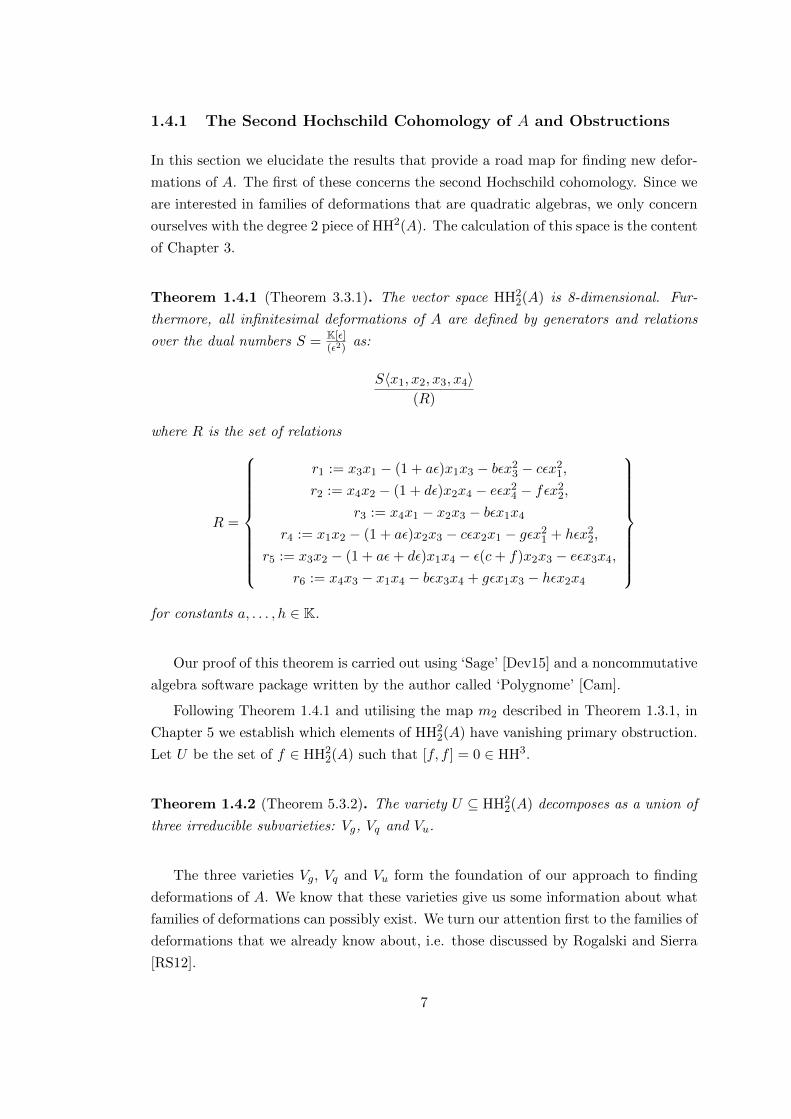
Theorem 1.4.1 (Theorem 3.3.1). The vector space HH22(A) is 8-dimensional. Fur-
thermore, all infinitesimal deformations of A are defined by generators and relations
over the dual numbers S = K[ε](ε2)
as:
S〈x1, x2, x3, x4〉(R)
where R is the set of relations
R =
r1 := x3x1 − (1 + aε)x1x3 − bεx23 − cεx2
1,
r2 := x4x2 − (1 + dε)x2x4 − eεx24 − fεx2
2,
r3 := x4x1 − x2x3 − bεx1x4
r4 := x1x2 − (1 + aε)x2x3 − cεx2x1 − gεx21 + hεx2
2,
r5 := x3x2 − (1 + aε+ dε)x1x4 − ε(c+ f)x2x3 − eεx3x4,
r6 := x4x3 − x1x4 − bεx3x4 + gεx1x3 − hεx2x4
for constants a, . . . , h ∈ K.
Our proof of this theorem is carried out using ‘Sage’ [Dev15] and a noncommutative
algebra software package written by the author called ‘Polygnome’ [Cam].
Following Theorem 1.4.1 and utilising the map m2 described in Theorem 1.3.1, in
Chapter 5 we establish which elements of HH22(A) have vanishing primary obstruction.
Let U be the set of f ∈ HH22(A) such that [f, f ] = 0 ∈ HH3.
Theorem 1.4.2 (Theorem 5.3.2). The variety U ⊆ HH22(A) decomposes as a union of
three irreducible subvarieties: Vg, Vq and Vu.
The three varieties Vg, Vq and Vu form the foundation of our approach to finding
deformations of A. We know that these varieties give us some information about what
families of deformations can possibly exist. We turn our attention first to the families of
deformations that we already know about, i.e. those discussed by Rogalski and Sierra
[RS12].
7
1.4.2 Families of Deformations Arising from Automorphisms of Sur-
faces
The families of deformations discovered by Rogalski and Sierra are constructed by
deforming Qgr(A), the graded quotient ring of A. By work of Yekutieli and Zhang
[YZ06], Qgr(A) is isomorphic to K(u, v)[t, t−1;σ], where σ is a certain automorphism
of K(u, v). If we are to find new families of deformations, we certainly want to avoid
rediscovering those families that are already well understood. For this reason, we
establish which elements of HH22 appear as infinitesimals of these previously studied
families.
Rogalski and Sierra restricted their attention to deformations of Qgr(A) of the form
K(u, v)[t, t−1;σ ◦ τ ],
where τ is the pull back of some automorphism of the surface P1 × P1. In Chapter 6
we examine the more general case of τ being an automorphism of any minimal rational
surface, in the hopes of finding families with distinct infinitesimals.
Since Qgr(A) is a localisation of A, and A is a Koszul domain, we may apply
Theorem 1.3.2 in order to determine which infinitesimals are tangent to these families.
The combined result of this work is the following.
Theorem 1.4.3 (Theorems 6.4.1, 6.5.1 and 6.6.2). The deformations of A arising from
automorphisms of minimal rational surfaces correspond to the space of infinitesimal
deformations Vg. Furthermore, the set of deformations studied by Rogalski and Sierra
comprises all of Vg.
This result is a signal that in order to find new families of deformations of A, one
must concentrate on those families whose infinitesimals lie in Vq and Vu. The rest of
the results concern such deformations.
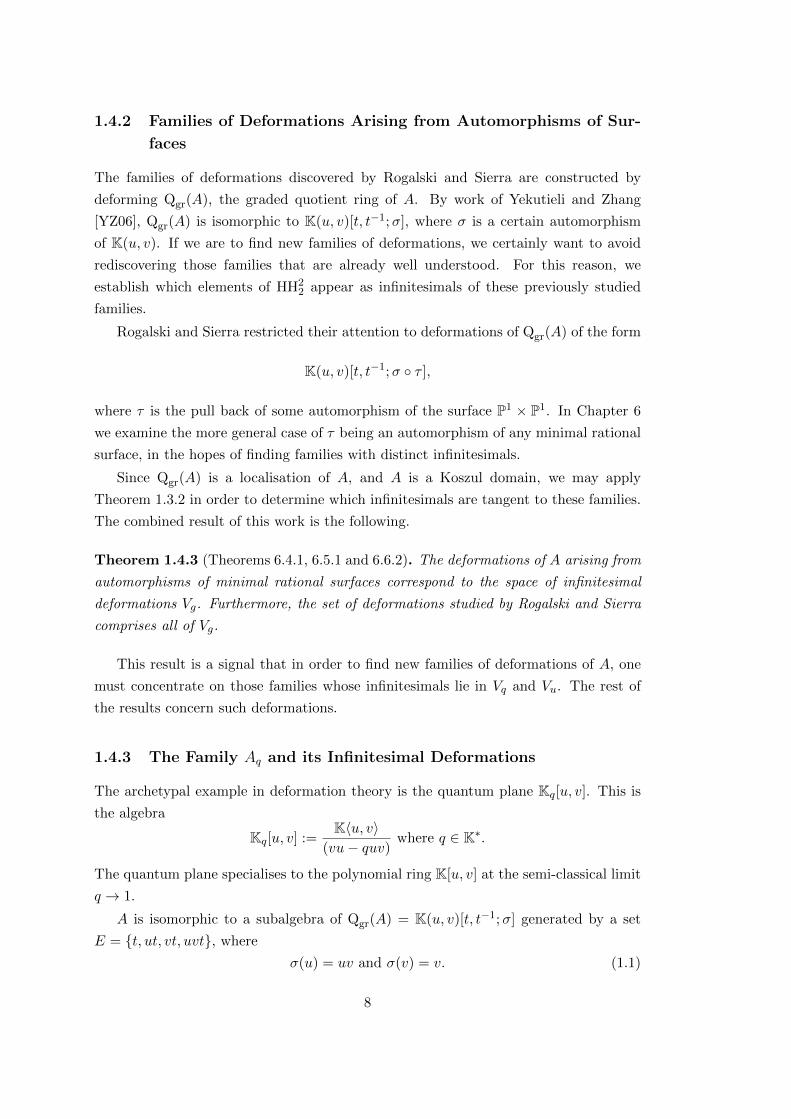
1.4.3 The Family Aq and its Infinitesimal Deformations
The archetypal example in deformation theory is the quantum plane Kq[u, v]. This is
the algebra
Kq[u, v] :=K〈u, v〉
(vu− quv)where q ∈ K∗.
The quantum plane specialises to the polynomial ring K[u, v] at the semi-classical limit
q → 1.
A is isomorphic to a subalgebra of Qgr(A) = K(u, v)[t, t−1;σ] generated by a set
E = {t, ut, vt, uvt}, where
σ(u) = uv and σ(v) = v. (1.1)
8

Let Kq(u, v) be the full division ring of Kq[u, v]. The equations (1.1) also define an
automorphism of Kq(u, v). Therefore we may define a family of algebras generated by
Eq = {t, ut, vt, uvt} in the graded division ring
Kq(u, v)[t, t−1;σ].
We call this family of algebras Aq, and prove that the family Aq is a family that deforms
A in Corollary 3.4.2.
Using similar methods to those of Theorems 1.4.1 and 1.4.2, in Chapters 3 and 5
we find the following theorem.
Theorem 1.4.4 (Theorem 3.4.3 and Proposition 5.4.1).
1. HH22(Aq) is a four dimensional space.
2. All infinitesimal deformations of Aq have vanishing primary obstruction.
We use Aq to generate more families of A by mimicking the work of Rogalski and
Sierra. Since Kq(u, v) is noncommutative, it is not the function field of any projective
surface. However, there is work of Alev and Dumas [AD95] that describes subgroups
of Kq(u, v) that are quantum analogues to certain automorphism groups of projective
surfaces. We define families of deformations of Aq by taking appropriate subalgebras
of
Kq′(u, v)[t, t−1;σ ◦ τ ]
for τ an automorphism arising from these ‘quantum’ geometric automorphism groups.
Unlike in the case of A, these families have infinitesimals that comprise all of HH22(Aq).
Theorem 1.4.5 (Theorem 7.3.1). For every isomorphism class of infinitesimal de-
formations L of Aq there exists a family of deformations of Qgr(Aq) such that the
associated infinitesimal F1 satisfies:
[F1|Rq ] = L.
Once these families are described, we take the semi-classical limit q → 1 and find
that these families provide new families of deformations of the algebra A.
Proposition 1.4.6 (Proposition 7.3.2). The semi-classical limits of the families of
deformations of Aq arising from quantum geometric automorphisms correspond to a 2
dimensional subspace of infinitesimal deformations of A lying in Vq.
1.4.4 A Family of Deformations of A with the PBW Property
The final result in the thesis is that we define a new family of deformations of A all
of whose elements satisfy the PBW property. In order to find this family, we carried
9

out a heuristic search of the space Vq for cocycles that would define such a family. The
details of this search are beyond the scope of this summary. The main result of Chapter
8 is the following.
Theorem 1.4.7 (Theorem 8.2.1, Corollary 8.2.8 and Corollary 8.2.3). Let
A(a, c, d, f) :=K〈x1, x2, x3, x4〉
(Ra,c,d,f )
where a, c, d, f ∈ K and Ra,c,d,f is the set of relations
Ra,c,d,f =
r1 := x3x1 − (1 + a)x1x3 − cx2
1, r2 := x4x2 − (1 + d)x2x4 − fx22,
r3 := x4x1 − (1 + d)x2x3 − fx2x1, r4 := x1x2 − x2x3,
r5 := x3x2 − (1 + a)x1x4 − cx2x3, r6 := x4x3 − (1 + a)x1x4 − cx2x3
.
If af − cd = 0 and a 6= −1 6= d then A(a, c, d, f) is a non-noetherian GK-dimension 4
domain that is PBW with respect to the lexicographic ordering induced by x2 < x1 <
x3 < x4.
In particular we establish that A(a, c, d, f) is a flat family of algebras deforming A.
Theorem 1.4.8 (Corollary 8.2.2). A(a, c, d, f) is a flat family of algebras deforming
A over the ringK[a, c, d, f, 1
1+a ,1
1+d ]
(af − cd).
We analyse this family further by describing the function skew field, and thereby
classifying these algebras up to birational equivalence. In particular, we demonstrate
that A(a, c, d, f) is a GK-dimension 4 noncommutative surface.
Theorem 1.4.9 (Corollary 8.2.7 and Proposition 8.2.9). The function skew field of
A(a, c, d, f) is isomorphic to
1. Kq(u, v) where q = 1+d1+a if a 6= d.
2. D1(K), the division ring of the first Weyl algebra, if a = d = 0 and f 6= c.
3. K(u, v) if a = d and c = f .
The methods used to find this family are interesting in their own right, but fail
to yield results for infinitesimal deformations lying in the variety Vu. However, since
Vq ∩ Vu and Vu ∩ Vg are large subvarieties in Vu, we have already seen several families
of algebras whose infinitesimal lies in Vu. In conclusion, we have seen families whose
infinitesimals comprise all of Vg, a substantial portion of Vq and large subvarieties of
Vu.
10

1.5 Further Work
1.5.1 The map m∗
In the setting of PBW algebras we may apply basic homological algebra and deduce that
there exist maps mn for all n ∈ N that extend m2 to the entire bar resolution. Although
we have not discussed this explicitly, our work in Chapter 4 implies an algorithm for
calculating a continuation to B3 of m2 by taking ‘paths’ of 2-cells in the Bergman graph.
It is a firm belief of the author that the maps mn may be defined algorithmically by
taking choices of sequences of n-cells in the Bergman graph that have as boundary
(n− 1)-cells that are specified by the choice of mn−1.
The more general problem of finding a map φ∗ : B∗ → K∗ for Koszul algebras is
interesting and known to be difficult. The map m2 provides an obvious starting point
for further study. The combinatorial theory underlying the Bergman Diamond Lemma
is well known in computer science, where an almost identical theorem known as the
Church-Rosser theorem is fundamental in the theory of λ-calculus. In the λ-calculus
theory there are situations where the diamond lemma only holds for certain subsets of
the ‘terms’ under study. This failure reflects somewhat the difference between a general
Koszul algebra and a PBW algebra and there may be already developed theory that
one may apply in the setting of noncommutative algebras.
1.5.2 Deformations of A
There are immediate questions for investigation in the family A(a, c, d, f). None of the
algebras in this family are noetherian, in contrast to those examined by Rogalski and
Sierra. It would be extremely surprising if they were AS-Gorenstein as none of those in
the Rogalski-Sierra family had this property. These algebras are an obvious launching
point for further work on GK-dimension 4 noncommutative surfaces.
Turning to A, we have not discussed the formal deformations of A for the most part
as our aims have been realising flat families over non-local rings. However, we have ev-
idence that many of the infinitesimal deformations with vanishing primary obstruction
integrate to formal deformations. An interesting property for algebras to have is that
infinitesimal deformations integrate if and only if they have vanishing primary obstruc-
tion. This would be worth investigating in A, and the classification of the infinitesimal
deformations in Chapter 5 would provide a useful starting point for such work.
As for other families of deformations over non-local rings, we conjecture that there
exist families of algebras that deform A with associated infinitesimals that cover all
of Vq. We have discussed in Chapter 8 that answering this question will require new
techniques as the resulting algebra cannot be PBW with the specified basis that we
have studied.
11
Finally, are there any flat families of algebras whose associated infinitesimal lies in
Vu? We have been unable to answer this question, except in the case of the overlaps
with Vq and Vg. The author believes the answer to be positive, but this is not based
on anything but optimism. The main conjecture we make about any such algebras is
that they will have function skew field that is isomorphic Kq(u, v) for some q. This
reasoning behind this is that the generic element of all the families discussed in the
thesis has such a skew field. These algebras are worth investigation not least because
examples of transcendence degree 2 division rings ‘in the wild’ are of interest as testing
grounds for the theory of noncommutative surfaces and Artin’s conjecture.
12

Chapter 2
Background
In this chapter we present the background material, theory and theorems upon which
the rest of the thesis is based. In particular we will provide an overview of the funda-
mentals of algebraic deformation theory, the theory of Koszul and PBW algebras, and
introduce the algebra A that will play a key role in the thesis.
Notation 2.0.1. We adopt the global convention that K is a field and unadorned
tensor products are to be considered as tensor products over K. Furthermore, we will
sometimes use the symbol | for the tensor product ⊗K.
2.1 Koszul Algebras
First introduced by Priddy [Pri70], Koszul algebras have proved fertile ground for
research. The motivation in studying them has been that whilst they are a large class
of quadratic algebras, their behaviour is considerably less wild than the general case.
The definitive text on Koszul algebras is by Polishchuk and Positelskei [PP05], although
we also take definitions from [BG96] as they are more suited to the work in this thesis.
Definition 2.1.1. For a K-algebra C we call the K-algebra Ce := C ⊗K Cop the
enveloping algebra of C.
The useful property of enveloping algebras is that the category of C-bimodules is
equivalent to the category of right Ce-modules.
Before considering Koszul algebras themselves, we define the bar resolution which
plays a central role in deformation theory and will appear throughout the thesis.
Definition 2.1.2. For a K-algebra C, let Bn(C) be the C-bimodule C⊗n+2, which we
often just write as Bn if the context is clear. We define the bar (or standard) resolution
of C to be the complex of right Ce-modules
B∗ → C,
13

where the boundary map bn : Bn → Bn−1 is given by
bn(c0 ⊗ c1 ⊗ . . .⊗ cn ⊗ cn+1) = c0c1 ⊗ c2 ⊗ . . .⊗ cn+1
+∑i
(−1)ic0 ⊗ . . .⊗ cici+1 ⊗ . . .⊗ cn+1
+ (−1)n+1c0 ⊗ c1 ⊗ . . .⊗ cncn+1,
and the final map C ⊗ C → C is the multiplication map.
Note that the above definition is completely general and requires no assumptions
about the structure of C. From this point forwards however, we will be dealing only
with quadratic algebras.
Notation 2.1.3. If V is a finite set then we denote by T (V ) the tensor algebra on
spK(V ). Note that T (V ) =⊕
i T (V )i is a graded algebra with each generator lying in
T (V )1.
Definition 2.1.4. For a set of relations R ⊆ spK(V )⊗ spK(V ) we consider an algebra
C :=K〈V 〉(R)
.
Since R ⊆ T (V )2, C is N-graded and we write this grading as
C =⊕i∈N
Ci.
The Koszul complex is given by Kn = C ⊗Kn ⊗ C, where Kn is defined as:
Kn =
K if n = 0
C1 if n = 1⋂n−2j=0 C
⊗j1 ⊗R⊗ C
⊗i−j−21 otherwise.
The inclusion of R into C1 ⊗ C1 gives a C-bimodule embedding in : Kn ↪→ Bn. The
differential of the Koszul complex is induced by restriction from that of the bar complex;
this is well defined since Im bn ◦ in ⊆ in−1(Kn−1).
An algebra is Koszul if the Koszul complex is a resolution of C as a right Ce-module.
Remark 2.1.5. There are many equivalent definitions of a Koszul algebra. We choose
a homological definition, since much of the work in the thesis is homological in nature.
For a comparison of other definitions of Koszul algebras we direct the reader to [BG96,
Appendix A].
14
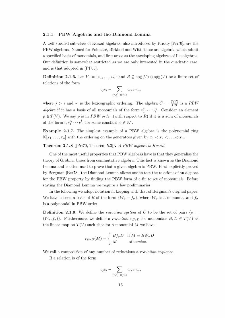
2.1.1 PBW Algebras and the Diamond Lemma
A well studied sub-class of Koszul algebras, also introduced by Priddy [Pri70], are the
PBW algebras. Named for Poincare, Birkhoff and Witt, these are algebras which admit
a specified basis of monomials, and first arose as the enveloping algebras of Lie algebras.
Our definition is somewhat restricted as we are only interested in the quadratic case,
and is that adopted in [PP05].
Definition 2.1.6. Let V := {v1, . . . , vγ} and R ⊆ spK(V ) ⊗ spK(V ) be a finite set of
relations of the form
vjvi −∑
(r,s)≺(j,i)
crsvrvs,
where j > i and ≺ is the lexicographic ordering. The algebra C := T (V )(R) is a PBW
algebra if it has a basis of all monomials of the form vi11 · · · viγγ . Consider an element
p ∈ T (V ). We say p is in PBW order (with respect to R) if it is a sum of monomials
of the form civi11 · · · v
iγγ for some constant ci ∈ K∗.
Example 2.1.7. The simplest example of a PBW algebra is the polynomial ring
K[x1, . . . , xn] with the ordering on the generators given by x1 < x2 < . . . < xn.
Theorem 2.1.8 ([Pri70, Theorem 5.3]). A PBW algebra is Koszul.
One of the most useful properties that PBW algebras have is that they generalise the
theory of Grobner bases from commutative algebra. This fact is known as the Diamond
Lemma and is often used to prove that a given algebra is PBW. First explicitly proved
by Bergman [Ber78], the Diamond Lemma allows one to test the relations of an algebra
for the PBW property by finding the PBW form of a finite set of monomials. Before
stating the Diamond Lemma we require a few preliminaries.
In the following we adopt notation in keeping with that of Bergman’s original paper.
We have chosen a basis of R of the form {Wσ − fσ}, where Wσ is a monomial and fσ
is a polynomial in PBW order.
Definition 2.1.9. We define the reduction system of C to be the set of pairs {σ =
(Wσ, fσ)}. Furthermore, we define a reduction rBσD for monomials B,D ∈ T (V ) as
the linear map on T (V ) such that for a monomial M we have:
rBσD(M) =
{BfσD if M = BWσD
M otherwise.
We call a composition of any number of reductions a reduction sequence.
If a relation is of the form
vjvi −∑
(r,s)≺(j,i)
crsvrvs,
15

then we label the associated element of the reduction system σj,i.
The idea of the Diamond Lemma is that in order to verify that a set of relations
defines a PBW algebra, one only needs to check that the PBW forms of a finite set of
monomials are unique.
Definition 2.1.10. If V and R are as in Definition 2.1.6 then an overlap ambiguity is
a degree 3 monomial of the form
vjvkvl with j > k > l.
By definition, for an overlap ambiguity w, there are two reductions one may apply
to w: rvjσk,l and rσj,kvl .
Definition 2.1.11. An overlap ambiguity w = vjvkvl is said to be resolvable if there
exist two reduction sequences rn · · · r1 and sm · · · s1 such that s1 = rvjσk,l , r1 = rσj,kvland
sm · · · s1(w) = rn · · · r1(w).
We are now ready to state the Diamond Lemma. Note that the version we use
is not as powerful as the original result as we are only interested in graded quadratic
algebras in this thesis. For this reason we have modified the theorem slightly.
Theorem 2.1.12 ([Ber78, Theorem 1.2]). If V and R are as in Definition 2.1.6, then
the algebra C = K〈V 〉(R) is PBW if and only if all overlap ambiguities are resolvable.
Example 2.1.13. We show using the Diamond Lemma that the algebra A defined in
Definition 1.1.1 is PBW with respect to the ordering given by x2 < x1 < x3 < x4. Note
that this was previously established by Rogalski and Sierra [RS12, Proof of Lemma
5.7]. The overlaps of A are precisely the monomials
{x4x1x2, x3x1x2, x4x3x2, x4x3x1}.
We show the resolution in full for x4x1x2 but only give the two sequences for the other
three cases.
1.
rx2r6rr2x3rx4r4(x4x1x2) = rx2r6rr2x3(x4x2x3) = rx2r6(x2x4x3) = x2x1x4
= rx2r5(x2x3x2) = rx2r5rr3x2(x4x1x2)
2.
rx1r6rr5x3rx3r4(x3x1x2) = x21x4 = rx1r5rr1x2(x3x1x2)
16

3.
rr3x4rx4r5(x4x3x2) = x2x3x4 = rr4x4rx1r2rr6x2(x4x3x2)
4.
rr3x3rx4r1(x4x3x1) = x2x23 = rr4x3rx1r3rr6x1(x4x3x1)
Since all four overlaps are resolvable, we can apply the Diamond Lemma and conclude
that A is PBW with the basis {xi2xj1xk3x
l4}.
2.2 The Algebra A
The main focus of this thesis is applying deformation theory to study algebras ‘close’
to the algebra A as defined in Definition 1.1.1. Before discussing A itself we provide
some context and definitions that will allow us to state fully the properties that A has
that we are particularly interested in.
2.2.1 Preliminary Definitions from Noncommutative Projective Ge-
ometry
In the field of noncommutative projective geometry the main idea is to generalise the
sheaf theoretic approach of modern algebraic geometry to noncommutative algebras.
We will not discuss the field in detail, as the technical heart of the thesis is Gersten-
haber’s deformation theory. However, many of the concepts are relevant. In particular,
the growth and dimension of a ring will be used throughout the thesis.
Gelfand-Kirillov Dimension
There are many definitions of dimension for noncommutative rings which go some way
to generalising commutative notions of dimension. The most relevant in this thesis is
Gelfand-Kirillov dimension.
Definition 2.2.1. The Gelfand-Kirillov dimension (hereafter GK-dimension) of an
algebra C is
GKdim(C) = supV
lim supn→∞
(logn(dimF(V n))),
where the supremum ranges over all finite dimensional subspaces V of C.
GK-dimension generalises Krull dimension in the sense that they agree for finitely
generated commutative domains. Unfortunately, GK-dimension has some bad proper-
ties in general. For example, for any real number r larger than 2, there is an algebra
with GK-dimension r [KL00, Theorem 2.9]. In the algebraic setting of this thesis the
GK-dimension of an algebra is strongly related to its Hilbert series.
17
Definition 2.2.2. For a graded K-algebra C =⊕
iCi the Hilbert series of C is the
power series
hC(p) =∑i
dim(Ci)pi.
In other words, hC(p) is the generating function for dim(Ci).
Lemma 2.2.3 ([Rog, Lemma 2.7]). Suppose that C =⊕
iCi is a graded algebra such
that C0 = K. If the Hilbert series of C is of the form hC(t) = 1/p(t), where p ∈ Z[t],
then C has finite GK-dimension if and only if all roots of p in the complex plane lie on
the unit circle. Moreover, in this case, the GK-dimension is an integer, and it is equal
to the multiplicity of vanishing of p(t) at t = 1.
Noncommutative Localisation
Localisation refers to the process of adding inverses to a ring. In the noncommutative
setting there are problems with naively inverting given sets of elements. the condition
required to avoid these issues is the Ore conditions.
Definition 2.2.4. A set S ⊆ C is a right Ore set with respect to a subset B ⊆ C if S
is a multiplicatively closed set such that for any a ∈ B and s ∈ S, there exist b ∈ Band r ∈ S such that the following holds:
ar = sb.
S is a right Ore set if B is the whole ring C. A left Ore set is defined in the same way
mutatis mutandis.
If S is a right Ore set in a domain C then we can consider the localisation of C at
S, which we define with a universal property.
Definition 2.2.5. For S a right Ore set in a domain C then the localisation of C at S
is written CS and is a ring with a homomorphism θ : C ↪→ CS satisfying the following
universal property: if R is a ring and φ : C → R is a ring homomorphism so that φ(s)
is a unit for every element s ∈ S, then φ factors through CS under θ.
The existence of a ring satisfying this property is the content of [MR01, Theorem
2.1.12]. Noncommutative localisation is the tool that allows us to consider birational
geometry in a noncommutative setting.
Noncommutative Birational Equivalence
Noncommutative birational equivalence generalises the commutative notion of bira-
tional equivalence between two projective varieties to noncommutative graded domains.
18

Definition 2.2.6. For C a graded domain of finite GK-dimension we define the graded
quotient ring
Qgr(C) := C〈h−1| 0 6= h ∈ C is homogeneous〉
It is not immediately obvious that such a ring is well defined, in that localisation
in noncommutative rings depends on the Ore condition being satisfied. This can be
verified by combining [NvO82, Theorem C.I.1.6] and [KL00, Theorem 4.12].
The utility of this construction arises from the following theorem.
Theorem 2.2.7 ([NvO82, Theorems A.I.5.8 and C.I.1.6]). For C a graded domain of
finite GK-dimension, there exists a division ring D and τ an automorphism of D such
that
Qgr(C) ∼= D[t, t−1; τ ].
Definition 2.2.8. We call the division ring D in Theorem 2.2.7 the function skew field
of C. We will often refer to this simply as the function field by abuse of language,
although we remind the reader that this is not intended to suggest D is commutative.
Two algebras are said to be birationally equivalent if they have isomorphic function
skew fields.
Definition 2.2.9. We call a finitely generated graded K-algebra C =⊕
iCi with C0 =
K finitely graded . A finitely graded domain with a function skew field of transcendence
degree 2 over the ground field K is called a noncommutative projective surface or simply
a noncommutative surface.
Classifying noncommutative surfaces is an open and difficult problem, even up to
birational equivalence (see [SVdB01]). One particularly well understood class of non-
commutative surfaces are the birationally commutative surfaces.
Definition 2.2.10. If a finitely graded domain has a function field that is commutative
then we call it birationally commutative. We will refer to noncommutative projective
surfaces that are birationally commutative as birationally commutative surfaces.
2.2.2 Definition of A and Basic Properties
Although A was first defined by Yekutieli and Zhang in [YZ06, Section 7] as a subgroup
of a group algebra, we prefer to follow Rogalski and Sierra [RS12] and we have defined
A by a finite presentation in Definition 1.1.1.
The following result is due to Smith and Zhang, although the proof is not published,
and establishes many of the basic properties of A. Note that although due to Smith
and Zhang, the result was published in a paper of Yekutieli and Zhang.
Proposition 2.2.11 ([YZ06, Proposition 7.6]). A is a finitely graded K-algebra with
the following properties.
19

(a) A is a Koszul algebra.
(b) A is a domain with Hilbert series
hA(p) =1
(1− p)4.
(c) A is neither left nor right noetherian.
Note that we have already established Part (a) of Proposition 2.2.11 in Example
2.1.13 since PBW algebras are Koszul by Theorem 2.1.8. Of particular interest from a
noncommutative geometry perspective is the following birational classification of A.
Notation 2.2.12. For a set X the symbol K〈X〉 is used to denote the subalgebra
generated by X if X is a subset of a K-algebra and the free algebra on X otherwise. It
will be clear from the context which is meant.
Proposition 2.2.13 ([YZ06, Proposition 7.8 and its proof]). A is a GK-dimension 4
birationally commutative surface. In particular, there exists a isomorphism:
Qgr(A) ∼= K(u, v)[t, t−1;σ]
where σ ∈ Aut(K(u, v)) is defined by
σ(u) = uv and σ(v) = v.
Indeed, A is embedded in Qgr(A) in the following manner:
Lemma 2.2.14 ([RS12, Lemma 5.7 (i)]). Let E := {t, ut, vt, uvt}. Then the map
φ : A→ K(u, v)[t, t−1;σ] given by
φ(x1) = t, φ(x2) = ut, φ(x3) = vt, φ(x4) = uvt
defines an isomorphism:
A ∼= K〈E〉.
This particular embedding of A into Qgr(A) is a useful tool that will appear through-
out the thesis. There are several properties of A that are best understood when con-
sidering A as a subalgebra of Qgr(A), whereas the presentation of A given in Definition
1.1.1 is often easier to make calculations with.
2.2.3 Deformations Of A
By basic theory from birational geometry [Har77, Theorem 4.4], the automorphism
σ ∈ Aut(K(u, v)) defined in Proposition 2.2.13 defines a birational self-map for any
20
rational surface. Rogalski and Sierra consider one such birational self-map in [RS12].
In the following we abuse notation and write σ for both the automorphism of K(u, v)
and the birational map of P1 × P1.
Definition 2.2.15. Define the birational map σ : P1 × P1 99K P1 × P1 by
σ([x : y][z : w]) = [xz : yw][z : w].
Then choose the chart on P1 × P1 given by u = x/y and v = z/w.
It is immediate that this choice of chart on P1×P1 corresponds to the automorphism
of K(u, v) defined in Proposition 2.2.13. The paper [RS12] concerns families of algebras
that ‘deform’ A by certain a set of automorphisms {τ} ⊆ Aut(P1 × P1).
Definition 2.2.16. If τ ∈ Aut(P1 × P1) then consider the set
E(τ) := {t, ut, vt, uvt} ⊆ K(u, v)[t;σ ◦ τ ].
Then define A(τ) to be the algebra K〈E(τ)〉.
Intuitively, one expects A(τ) to be an algebra with similar properties to A. In
fact the main theorem of [RS12] is that whilst it is true that (for certain τ) A(τ) has
GK-dimension 4, almost all of these algebras are noetherian.
Theorem 2.2.17 ([RS12, Theorem 1.6]). There exists a subgroup of automorphisms
in Aut(P1 × P1) comprised of elements τ = τ(ρ, θ) parametrised by ρ, θ ∈ K, such that
if ρ and θ are algebraically independent over the prime subfield of K then A(τ) is a
GK-dimension 4 noetherian finitely graded domain which is Koszul.
This theorem was surprising since at the time no examples of noetherian birationally
commutative surfaces were known to exist in GK-dimension 4. The algebras A(τ) can
be considered as deformations of A in an obvious way. One goal of this thesis is to
discover whether or not there are other families of algebras that deform A.
2.3 Deformation Theory
The theory of formal deformations of algebras was first introduced by Gerstenhaber
[Ger64], and has had wide ranging impact in both mathematics and physics. Inspired
by ideas from analytic deformation theory [KNS58, KS58] and examples from quantum
mechanics [Moy49], Gerstenhaber defined families of algebras that can be thought of
as ‘close’ to a given algebra.
There are several readable surveys of Gerstenhaber’s deformation theory available.
Szendroi has written a very readable introduction with applications to Calabi-Yau
21
manifolds in [Sze99]. However, for more detailed and algebraic considerations of the
theory the reader is directed to [Fox93] for an introduction and [Gia11] for a high level
historical survey. Furthermore, the original papers by Gerstenhaber [Ger63, Ger64] are
still extremely relevant and accessible.
2.3.1 Hochschild Cohomology
The main thrust of Gerstenhaber’s foundational papers [Ger63, Ger64] is that the
deformation theory of a K-algebra is intimately related to its Hochschild cohomology.
Furthermore, the Hochschild cohomology comes with a wealth of algebraic structures
defined upon it and these also have relation to the deformation theory of the algebra in
question. For that reason we first define Hochschild cohomology, which was introduced
by Hochschild in [Hoc45].
Definition 2.3.1. The Hochschild cohomology of a K-algebra C, written HH∗(C), is
the homology of the dual complex to the bar complex (see Definition 2.1.2). That is to
say that it is the cohomology of the bar complex under the contravariant functor
HomCe(−, C).
Example 2.3.2. 1. HH0(C) is the centre of the algebra C. To see this, note that
f ∈ HomCe(C⊗2, C) is determined by f(1⊗1) = c ∈ C so that HomCe(C
⊗2, C) ∼=CCe . Then f is a Hochschild 0-cocycle if and only if for every d ∈ C
b1(f)(1⊗ d⊗ 1) = f(d⊗ 1)− f(1⊗ d) = dc− cd = 0.
Therefore f is a cocycle if and only if c is central.
2. HH1(C) is the quotient of the group of derivations of C by the group of inner
derivations of C.
Of course, by the Comparison Theorem [Wei94, Theorem 2.2.6] the explicit depen-
dence on the bar complex in the definition of Hochschild cohomology is illusory, in
that HH∗(C) ∼= Ext∗Ce(C,C). One could replace this resolution with any other projec-
tive resolution of C as a right Ce-module and the resulting cohomology would be the
same. Indeed, much of the work in this thesis depends upon that fact. However, there
are several algebraic structures defined on the bar complex that have significance in
Gerstenhaber’s theory of formal deformations, as we shall shortly see.
2.3.2 Deformations
Definition 2.3.3. Let R be a K-algebra with an augmentation map R → K so that
K has a canonical R-module structure. For a K-algebra C we define a flat family of
22

algebras that deforms C over R to be a flat R-algebra AR with an algebra isomorphism
AR ⊗R K ∼= A.
We define a formal deformation of C to be a flat family of algebras that deforms C
over R = K[[s]]. Equivalently, a formal deformation of C is an associative K[[s]]-algebra
structure on the K[[s]] vector space Cs := C⊗K[[s]] with an isomorphism of K-algebras
Cs(s)∼= C.
Intuitively, one can think of a formal deformation of an algebra as a one-parameter
family of algebras such that for any choice of q ∈ K one obtains a new algebra Cs(s−q) .
Unfortunately, in general this raises issues of convergence that are best left aside. How-
ever, we can certainly write the algebra structure on Cs = C⊗K[[s]] as a power series
which proves useful.
Definition 2.3.4. A formal deformation of a K-algebra C is defined by an associative
K[[s]]-bilinear map F : Cs ⊗K[[s]] Cs → Cs which is given on elements of a, b ∈ C by
F (a, b) =∑i
Fi(a, b)si,
where each Fi is a bilinear map on C. By the definition of a formal deformation we
know that F0(a, b) = ab, i.e. F0 is the multiplication map of C. We call the first Fi
that is nonzero for i > 0 the infinitesimal of F . By an abuse of language, we will often
refer to the power series F as a formal deformation.
An infinitesimal is best thought of as a tangent vector lying in the tangent space
to some moduli space of algebras. Using noncommutative differentials one can make
this statement more formal and accurate [Art96, Section 9], but the intuition suffices
for this thesis.
Now we repeat the definition of formal deformation, but this time over the ringK[[s]](si)
.
Definition 2.3.5. For any i ∈ N≥0, an ith level deformation of K-algebra C is an
associative K[[s]](si)
-algebra structure on C(i)s := C ⊗ K[[s]]
(si), given by a K[[s]]
(si)-bilinear map
F ′, with an isomorphism
C(i)s
(s)∼= C.
One can think of ith level deformations of an algebra C as approximations of formal
deformations for C. However, one should be aware that it is not always true that an
ith level deformation arises as Cs(si)
for some formal deformation structure on Cs.
Definition 2.3.6. A homomorphism of formal (respectively ith level) deformations
from F to G is a K[[s]] (resp. K[[s]](si)
) bilinear map, Φ, on Cs (resp. C(i)s ) so that the
23

following diagram commutes:
Cs Cs
C
Φ
With this definition of morphisms, formal deformations form a category E and ith
level deformations form a category Ei. We also naturally obtain functors E → Ei for all
i ∈ N and Ej → Ei for any pair i, j ∈ N with i < j arising from the canonical quotient
maps
K[[s]]→ K[[s]]
(si)and
K[[s]]
(sj)→ K[[s]]
(si).
The category E2 is of particular interest.
Definition 2.3.7. A 2nd level deformation F ′ is called an infinitesimal deformation.
Furthermore, let F ′1 : C ⊗ C → C be the linear map in the expansion of F ′ as a series,
so that for all a, b ∈ CF ′(a, b) = ab+ F ′1(a, b)s ∈ C(2)
s .
Then by a further abuse of language we refer to F ′1 as an infinitesimal deformation.
Note that F ′1 ∈ B2, the space of Hochschild 2-cochains.
The following proposition is a reformulation of the fact that a functor E → E2 exists.
Proposition 2.3.8 ([Ger64, Section 1]). An infinitesimal of a formal deformation of
C is an infinitesimal deformation of C.
We now come to the first connection to Hoschshild cohomology. Recall that we
would like to think of infinitesimals of a formal deformation as tangent vectors to some
moduli space of algebras. The following fundamental theorem is a statement of the fact
that this tangent space is precisely the second Hochschild cohomology space.
Proposition 2.3.9 ([Ger64, Section 1]). An infinitesimal deformation is a Hochschild
2-cocycle. Furthermore, two infinitesimal deformations are isomorphic in the sense of
Definition 2.3.5 if and only if they are cohomologous in Hochschild cohomology.
2.3.3 Integrating Deformations
We turn to the question of whether something akin to a converse of Proposition 2.3.8
ever holds true. More generally, we ask when is an object in Ei the image of some
object in E under the functor E → Ei. Since
K[[s]] ∼= lim←−K[[s]]
(si),
24
this question can be approached by answering the weaker question of when does an
object in Ei lie in the image of some object in Ei+1.
Definition 2.3.10. If F (a, b) =∑i
j Fj(a, b)sj is an ith level deformation of C then we
say F integrates to an (i+1)st level deformation if there exists an Fi+1 ∈ HomK(C⊗2, C)
such that
F ′(a, b) =i+1∑j
Fj(a, b)sj
is an (i+ 1)st level deformation.
We will see that the answer to this question is once again related to the Hochschild
cohomology of the algebra in question. However, we must first define some terms. The
following proposition is simply a reformulation of the fact that a formal deformation
defines an associative algebra structure. Note that in the case i = 1 this proposition is
a restatement of Proposition 2.3.8.
Proposition 2.3.11 ([Ger64, Section 1]). If F =∑
i Fisi is a formal deformation of
C then for each i ∈ N and every a, b, c ∈ C the following equation holds:∑p+q=i
Fp(Fq(a, b), c)− Fp(a, Fq(b, c)) = 0. (νi)
We can rewrite this formula as:∑p+q=ip,q>0
Fp(Fq(a, b), c)− Fp(a, Fq(b, c)) = aFi(b, c)− Fi(ab, c) + Fi(a, bc)− Fi(a, b)c
= b2(Fi)(a, b, c). (ν ′i)
For this reason, the expression on the left hand side of equation (ν ′i) is of particular
interest as its value controls whether or not an Fi can exist that integrates a given
(i− 1)st level deformation.
Definition 2.3.12. For any i ∈ N≥1, we call the expression∑p+q=ip,q>0
Fp(Fq(a, b), c)− Fp(a, Fq(b, c))
the associator of the (i− 1)st level deformation F =∑i−1
j Fjsj .
The following proposition takes the problem of integration and places it firmly into
the realm of Hochschild cohomology.
Proposition 2.3.13 ([Ger64, Proposition 3]). The associator is a Hochschild 3-cocycle.
25
Definition 2.3.14. For an ith level deformation F we call the cohomology class of
the associator the obstruction of F . In the case of an infinitesimal deformation, we
call the obstruction the primary obstruction. If G is the associator of an infinitesimal
deformation F1 then the primary obstruction is by definition the cohomology class of
G(a, b, c) = F1(F1(a, b), c)− F1(a, F1(b, c)).
From this it immediately follows from (ν ′i) that an ith level deformation integrates
to an (i + 1)st level deformation if and only if its associator is a coboundary (i.e. is
cohomologous to 0).
2.3.4 The Gerstenhaber Bracket
The final piece of technology we require is the Gerstenhaber bracket. Gerstenhaber
defined several interrelated functions on the bar complex, the full content of which is
beyond the scope of this overview. However, what is relevant here is that there is a
graded Lie algebra structure on the bar complex B∗ which is usefully connected to the
question of integration of ith level deformations.
Definition 2.3.15. For 0 ≤ i ≤ n let ◦i : Bn⊗Bm → Bn+m−1 be the map defined for
f ∈ Bn and g ∈ Bm by
f◦ig(c0⊗c1⊗. . .⊗cn+m) = f(c0⊗. . .⊗ci−1⊗g(1⊗ci⊗. . .⊗ci+m⊗1)⊗ci+m+1⊗. . .⊗cn+m).
Then f ◦g =∑
i(−1)(m−1)if ◦i g defines a bilinear map on B∗, which in turn defines
the Gerstenhaber bracket given by:
[f, g] = f ◦ g − (−1)(n−1)(m−1)g ◦ f.
Proposition 2.3.16 ([Ger63, Theorems 1 and 4]). The Gerstenhaber bracket defines
a graded Lie algebra structure on the bar complex that descends to a graded Lie algebra
structure on Hochschild cohomology.
The main theorem regarding this bracket is the following, which relates the question
of integration of deformations to the cohomology of the Gerstenhaber bracket of certain
elements.
Proposition 2.3.17. An ith level deformation integrates to an (i+ 1)st level deforma-
tion if and only if ∑p+q=ip,q>0
[Fp, Fq]
is a coboundary in B3.
26

In particular, an infinitesimal deformation f has vanishing primary obstruction if
and only if [f, f ] is a coboundary.
27

28
Chapter 3
The Second Hochschild
Cohomology Space for Two
Algebras of Interest
3.1 Introduction
In this chapter we explain and carry out some calculations regarding the Hochschild
cohomology structure for two specific PBW algebras, A and Aq. Recall from Definition
2.3.1 that the Hochschild cohomology of an algebra C is ExtCe(C,C), where Ce is the
enveloping algebra of C as defined in Definition 2.1.1.
A classical result of Gerstenhaber (see Proposition 2.3.9) is that the second Hochschild
cohomology space HH2(C) parametrises the isomorphism classes of infinitesimal defor-
mations of C. In this thesis we study only graded deformations where the parameter
of deformation has degree 0. This means that we only need concern ourselves with
calculating the degree 2 component of the second cohomology space.
Throughout the chapter we make use of the PBW property of the algebras. Specif-
ically, since PBW algebras are Koszul we use the Koszul complex as the projective res-
olution of C in calculating ExtCe(C,C). The terms in the Koszul complex are finitely
generated and so make the calculations tractable by computer. Much of the leg work is
carried out using two symbolic algebra packages: for linear algebra calculations we use
‘Sage’ [Dev15] whereas for noncommutative algebra calculations we use ‘Polygnome’,
a Python [Ros95] package written by the author (see Appendix B). The code for these
calculations is included in Appendix A.1.
Throughout the discussion of computer calculations we will assume a basic un-
derstanding of object oriented programming concepts (objects, classes etc.) and will
not explain any Python syntax. For references on these topics we refer the reader to
[Ros95].
29

3.2 Calculations of Hochschild Cohomology Spaces
We consider a PBW algebra C. The Hochschild cohomology is calculated by a routine
Ext calculation as described for example in [Wei94, Chapter 3]. We include the details
of the calculation for completeness here as they are carried out by computer. The
Koszul resolution (see Definition 2.1.4) is denoted by Kn = C ⊗ Kn ⊗ C, with maps
kn : Kn → Kn−1. The dual complex is denoted by
Kn = HomCe(Kn, C)
with the chain map written as kn.
We will repeatedly make use of the isomorphism
HomCe(Kn, C) ∼= HomK(Kn, C) (3.1)
which arises naturally from the adjunction between the free right Ce-module functor
and the corresponding forgetful functor.
The calculation then will proceed as follows. Firstly, we choose bases for Kn for
n = 1, 2 and 3. By the isomorphism (3.1) this is equivalent to choosing a free generating
set for each of these Kn’s.
Once these generating sets are chosen, we form the matrix of kn for n = 2 and
n = 3. We use this to calculate the kernel of k3 and the image of k2 in degree two.
From bases of these two vector spaces we calculate a basis for the quotient space, which
is the second Hochschild cohomology space in degree two.
Notation 3.2.1. Our convention is to write elements of Kn as column vectors. If
Z = {z1, . . . , zm} is the chosen ordered free generating set of Kn then the vectorΘ1
...
Θm
represents the unique function in Kn that sends each 1 ⊗ zi ⊗ 1 to Θi ∈ A. This
determines the function completely because of the isomorphism (3.1).
3.2.1 Implementation Details
A full discussion of the source code of ‘Polygnome’ is beyond the scope of this thesis.
However, we will discuss here the details of how the boundary maps in the Koszul
resolutions are defined. We have made the full source code freely available in an online
repository [Cam]. The defining code for the boundary maps k_1 and k_3 (and their
30
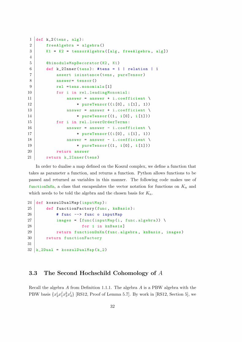
corresponding dual maps) can be found in Appendix B.1. We discuss k_2 and its dual
map as examples here.
The following code uses a decorator bimoduleMapDecorator. A decorator is a Python
class that modifies a function defined by the user in a predetermined way, perhaps
depending on some variables. In this case bimoduleMapDecorator takes as variables
the domain and codomain of a function between two free bimodules over an algebra.
The decorator allows the user to define a function on a bimodule generating set of the
domain and the program will automatically extend the function to the entire bimodule,
thereby reducing the amount of repetition in the source code.
Let C be a PBW algebra with generating space V and relation space R. Recall that
k2 has domain C ⊗R⊗ C and codomain C ⊗ V ⊗ C. In ‘Polygnome’ this information
is stored as both the codomain and domain being the tensorAlgebra C⊗F ⊗C, where
F is merely a placeholder that is implemented as the algebra with no relations.
Relations in ‘Polygnome’ are implemented in a class relation that allows the storage
of expressions of the form:
leadingMonomial = xy and lowerOrderTerms =∑
cif1i f
2i .
See Section 4.1 for a discussion of the notation used here. Since K2 has a free bimodule
generating set of the form {1 ⊗ (xy −∑cif
1i f
2i ) ⊗ 1} we define k_2 on this set only,
recalling that
k2(1⊗ (xy −∑
cif1i f
2i )⊗ 1) = x⊗ y ⊗ 1−
∑cif
1i ⊗ f2
i ⊗ 1
+ 1⊗ x⊗ y −∑
ci ⊗ f1i ⊗ f2
i .
31
1 def k_2(tens , alg):
2 freeAlgebra = algebra ()
3 K1 = K2 = tensorAlgebra ([alg , freeAlgebra , alg])
4
5 @bimoduleMapDecorator(K2, K1)
6 def k_2Inner(tens): #tens = 1 | relation | 1
7 assert isinstance(tens , pureTensor)
8 answer= tensor ()
9 rel =tens.monomials [1]
10 for i in rel.leadingMonomial:
11 answer = answer + i.coefficient \
12 * pureTensor ((i[0], i[1], 1))
13 answer = answer + i.coefficient \
14 * pureTensor ((1, i[0], i[1]))
15 for i in rel.lowerOrderTerms:
16 answer = answer - i.coefficient \
17 * pureTensor ((i[0], i[1], 1))
18 answer = answer - i.coefficient \
19 * pureTensor ((1, i[0], i[1]))
20 return answer
21 return k_2Inner(tens)
In order to dualise a map defined on the Koszul complex, we define a function that
takes as parameter a function, and returns a function. Python allows functions to be
passed and returned as variables in this manner. The following code makes use of
functionOnKn, a class that encapsulates the vector notation for functions on Kn and
which needs to be told the algebra and the chosen basis for Kn.
24 def koszulDualMap(inputMap ):
25 def functionFactory(func , knBasis ):
26 # func --> func o inputMap
27 images = [func(inputMap(i, func.algebra )) \
28 for i in knBasis]
29 return functionOnKn(func.algebra , knBasis , images)
30 return functionFactory
31
32 k_2Dual = koszulDualMap(k_2)
3.3 The Second Hochschild Cohomology of A
Recall the algebra A from Definition 1.1.1. The algebra A is a PBW algebra with the
PBW basis {xi2xj1xk3x
l4} [RS12, Proof of Lemma 5.7]. By work in [RS12, Section 5], we
32

know that the Koszul complex of A is isomorphic to:
0→ A[−4]→ A[−3]⊕4 → A[−2]⊕6 → A[−1]⊕4 → A→ 0.
With this in mind, to find the doubly defined relations (i.e. K3) we only need to give
four linearly independent elements of
V ⊗R ∩R⊗ V.
By observation one can see that the set
D :=
{d1 := x3r4 + x1(r6 − r5) = r1x2 − r5x3, d2 := x4r1 − x1r3 = r6x1 + (r4 − r3)x3
d3 := x4r5 − x1r2 = r6x2 + (r4 − r3)x4 d4 := x4r4 + x2(r6 − r5) = r3x2 − r2x3
}
is linearly independent and therefore provides a basis of K3.
We walk through the Sage script that calculates first the basis of Ker(k3)2 followed
by the basis of Im(k2)2. After some manipulations this allows us to read off a basis of
HH22(A).
3.3.1 Explanation of Computer Calculations
At the start of the script the variable bases is a list so that bases[i] is the PBW basis
for Ai and KnBases is a list so that KnBases[i] is the chosen generating set for Ki. The
first step is to build the generating set for K2 and K1. We include the K2 case here
as the code is almost identical in either case. Recall that functionOnKn is a class that
encapsulates the vector notation for functions on Kn and which needs to be told the
algebra and the chosen basis for Kn.
1 K2DualBasis = []
2 for i in range (6):
3 for element in bases [2]:
4 vectorRepresentation = [0] * i \
5 + [element] \
6 + [0] * (6-i-1)
7 function = functionOnKn(A,
8 KnBases [2],
9 vectorRepresentation)
10 K2DualBasis.append(function)
Now to find the kernel of k3 we form the matrix of k3 and use Sage to calculate a
basis of the kernel. Note that we must convert the vector representations from those
used internally by ‘Polygnome’ to those used by ‘Sage’ and vice versa. This is done
using the helper functions polygnomeVectorToSage and sageVectorToPolygnome. K is
defined as the field Q since we assume that K has characteristic 0.
33
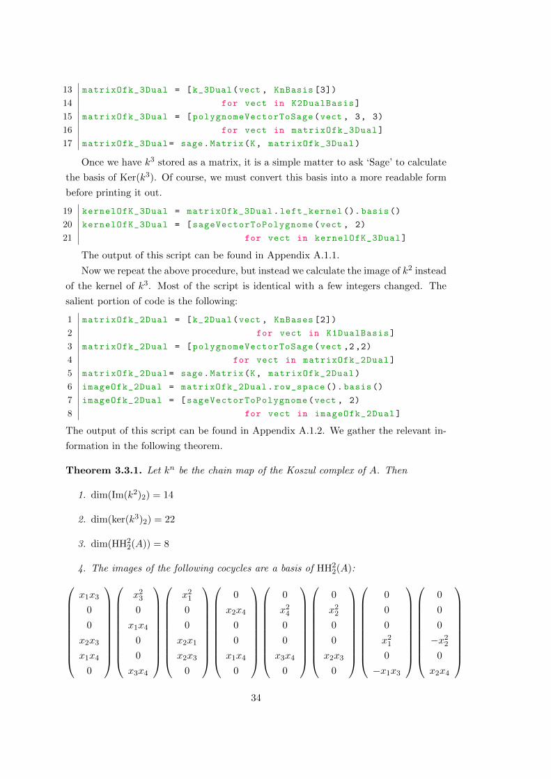
13 matrixOfk_3Dual = [k_3Dual(vect , KnBasis [3])
14 for vect in K2DualBasis]
15 matrixOfk_3Dual = [polygnomeVectorToSage(vect , 3, 3)
16 for vect in matrixOfk_3Dual]
17 matrixOfk_3Dual= sage.Matrix(K, matrixOfk_3Dual)
Once we have k3 stored as a matrix, it is a simple matter to ask ‘Sage’ to calculate
the basis of Ker(k3). Of course, we must convert this basis into a more readable form
before printing it out.
19 kernelOfK_3Dual = matrixOfk_3Dual.left_kernel (). basis ()
20 kernelOfK_3Dual = [sageVectorToPolygnome(vect , 2)
21 for vect in kernelOfK_3Dual]
The output of this script can be found in Appendix A.1.1.
Now we repeat the above procedure, but instead we calculate the image of k2 instead
of the kernel of k3. Most of the script is identical with a few integers changed. The
salient portion of code is the following:
1 matrixOfk_2Dual = [k_2Dual(vect , KnBases [2])
2 for vect in K1DualBasis]
3 matrixOfk_2Dual = [polygnomeVectorToSage(vect ,2,2)
4 for vect in matrixOfk_2Dual]
5 matrixOfk_2Dual= sage.Matrix(K, matrixOfk_2Dual)
6 imageOfk_2Dual = matrixOfk_2Dual.row_space (). basis()
7 imageOfk_2Dual = [sageVectorToPolygnome(vect , 2)
8 for vect in imageOfk_2Dual]
The output of this script can be found in Appendix A.1.2. We gather the relevant in-
formation in the following theorem.
Theorem 3.3.1. Let kn be the chain map of the Koszul complex of A. Then
1. dim(Im(k2)2) = 14
2. dim(ker(k3)2) = 22
3. dim(HH22(A)) = 8
4. The images of the following cocycles are a basis of HH22(A):
x1x3
0
0
x2x3
x1x4
0
x23
0
x1x4
0
0
x3x4
x21
0
0
x2x1
x2x3
0
0
x2x4
0
0
x1x4
0
0
x24
0
0
x3x4
0
0
x22
0
0
x2x3
0
0
0
0
x21
0
−x1x3
0
0
0
−x22
0
x2x4
34

The vector notation here is defined with reference to the chosen basis R above, as
discussed in Notation 3.2.1.
Proof. This follows directly from the preceding computer calculations. We have ordered
the output of the scripts discussed here in Appendices A.1.1 and A.1.2 so that the basis
of the cohomology space is easy to read off by eye.
3.4 A q-Deformation of A and its Second Hochschild Co-
homology
The central problem of the thesis is to find families of deformations of the algebra
A. We define here Aq, a one-parameter family of deformations of A that will be of
particular interest in Chapter 7. We shall see that the family Aq itself has families
of deformations which specialise to families of deformations of A in the semi-classical
limit q → 1. For that reason we record the details of the calculation of the degree two
component of the second Hochschild cohomology of Aq. Since the calculations of the
Hochschild cohomology of Aq are analogous to those for A we include them here.
3.4.1 Motivation
There are two methods of defining A that are both useful. The first, given in Section
3.3 is as a finitely presented algebra with four generators. However, another approach
is taken in [RS12], in which the authors start with the graded division ring
Qgr(A) = K(u, v)[t, t−1;σ]
where σ ∈ Aut(K(u, v)) is the map defined by
σ(u) = uv and σ(v) = v.
Then one may define A to be the subalgebra generated by
E := {x1 = t, x2 = ut, x3 = vt, x4 = uvt}.
We define Aq in two ways. Consider the quantum plane
kq[u, v] =K〈u, v〉vu− quv
for some q ∈ K∗
It is a basic fact in deformation theory that these algebras form a one-parameter family
of deformations of k[u, v]. One may define an automorphism σ′ of Kq(u, v) induced by
35
setting
σ′(u) = uv and σ′(v) = v. (3.2)
Since this satisfies:
σ′(vu) = σ′(v)σ′(u) = vuv = quv2 = qσ′(u)σ′(v) = σ′(quv)
in Kq(u, v), we can deduce that σ′ does indeed define an automorphism of Kq(u, v).
Since the defining equations (3.2) of σ′ are the same for that of σ ∈ Aut(K(u, v)), we
abuse notation and refer to both maps as σ with the algebra on which σ acts clear
by the context. We define the algebra Aq to be the subalgebra of Kq(u, v)[t, t−1;σ]
generated by Eq, where
Eq := {t, ut, vt, uvt} .
We will show that Aq is a quantised version of A in the sense that kq[u, v] is a
quantised affine plane, in particular Aq is a family of deformations of A.
3.4.2 Presentation of Aq
For a parameter q ∈ K∗ consider the algebra
A′q =K〈x1, x2, x3, x4〉
(Rq)
where Rq is the set consisting of the six relations
Rq =
{r1 := x3x1 − x1x3, r2 := x4x2 − qx2x4, r3 := x4x1 − x2x3
r4 := x1x2 − x2x3, r5 := x3x2 − qx1x4, r6 := x4x3 − x1x4
}.
By comparison with the definition of A it is clear that A′q is a PBW algebra with
the PBW basis {xi2xj1xk3x
l4} (see Section 3.3). Our next result is that Aq and A′q are
isomorphic.
Proposition 3.4.1. The algebras Aq and A′q are isomorphic. Furthermore, if K3 =
K3(Aq) then dim(K3) = 4.
Proof. We first show that Aq ∼= A′q by establishing that the map φ : Aq → A′q defined
by
x1 7→ t, x2 7→ ut, x3 7→ vt, x4 7→ uvt
is in fact an isomorphism of algebras.
A simple calculation shows that the elements in Eq satisfy the relations in Rq, so
that φ is a surjective algebra homomorphism. As for injectivity, we compare the Hilbert
series of the two algebras.
36
Since A′q is a PBW algebra with basis {xi2xj1xk3x
l4}, we know that
hA′q(p) =1
(1− p)4.
An argument similar to the proof of [RS12, Lemma 4.12 (1)] shows that the degree
d component of K〈Eq〉 has the following set as a basis:{uivjtd
∣∣∣ 0 ≤ i ≤ d, a(i) ≤ j ≤ b(i)},
where
a(i) =
(i
2
)and b(i) =
(d+ 1
2
)−(d− i
2
).
Thus
dimK(〈Eq〉d) =d∑i=0
[(d+ 1
2
)−(d− i
2
)−(i
2
)+ 1
]=
(d+ 3
3
),
which implies
h〈Eq〉(p) =1
(1− p)4.
Let V = spK(x1, x2, x3, x4). Note that the canonical mapping T (V ) → Aq is a
graded homomorphism. We know that Rq ⊗ V and V ⊗ Rq are both (6 × 4 = 24)-
dimensional, and that (Aq)3 is ((
63
)= 20)-dimensional. Recall that by definition
K3 = Rq ⊗ V ∩ V ⊗Rq
Therefore we have the following equations:
dim((Aq)3) = 20 = dim(T (V )3)− dim(Rq ⊗ V )− dim(V ⊗Rq) + dim(K3)
= 64− 24 ∗ 2 + dim(K3).
This implies that dim(K3) = 4 as required.
Corollary 3.4.2. Aq is a flat family of algebras over K[q] that deforms A.
Proof. This is a standard consequence of the fact that the Hilbert series of Aq is inde-
pendent of q [Har77, Theorem III.9.9].
As before, we can see that the set
Dq :=
{d1 := x3r4 + x1(qr6 − r5) = r1x2 − r5x3, d2 := x4r1 − x1r3 = r6x1 + (r4 − r3)x3
d3 := x4r5 − x1r2 = r6x2 + q(r4 − r3)x4 d4 := x4r4 + x2(qr6 − r5) = r3x2 − r2x3
}
is linearly independent and so provides a basis for K3.
37
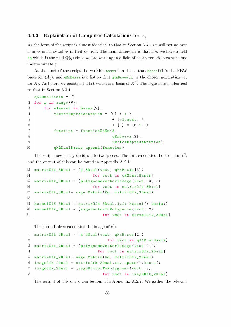
3.4.3 Explanation of Computer Calculations for Aq
As the form of the script is almost identical to that in Section 3.3.1 we will not go over
it in as much detail as in that section. The main difference is that now we have a field
Kq which is the field Q(q) since we are working in a field of characteristic zero with one
indeterminate q.
At the start of the script the variable bases is a list so that bases[i] is the PBW
basis for (Aq)i and qKnBases is a list so that qKnBases[i] is the chosen generating set
for Ki. As before we construct a list which is a basis of K2. The logic here is identical
to that in Section 3.3.1.
1 qK2DualBasis = []
2 for i in range (6):
3 for element in bases [2]:
4 vectorRepresentation = [0] * i \
5 + [element] \
6 + [0] * (6-i-1)
7 function = functionOnKn(A,
8 qKnBases [2],
9 vectorRepresentation)
10 qK2DualBasis.append(function)
The script now neatly divides into two pieces. The first calculates the kernel of k3,
and the output of this can be found in Appendix A.2.1.
13 matrixOfk_3Dual = [k_3Dual(vect , qKnBasis [3])
14 for vect in qK2DualBasis]
15 matrixOfk_3Dual = [polygnomeVectorToSage(vect , 3, 3)
16 for vect in matrixOfk_3Dual]
17 matrixOfk_3Dual= sage.Matrix(Kq, matrixOfk_3Dual)
18
19 kernelOfK_3Dual = matrixOfk_3Dual.left_kernel (). basis ()
20 kernelOfK_3Dual = [sageVectorToPolygnome(vect , 2)
21 for vect in kernelOfK_3Dual]
The second piece calculates the image of k2:
1 matrixOfk_2Dual = [k_2Dual(vect , qKnBases [2])
2 for vect in qK1DualBasis]
3 matrixOfk_2Dual = [polygnomeVectorToSage(vect ,2,2)
4 for vect in matrixOfk_2Dual]
5 matrixOfk_2Dual= sage.Matrix(Kq, matrixOfk_2Dual)
6 imageOfk_2Dual = matrixOfk_2Dual.row_space (). basis()
7 imageOfk_2Dual = [sageVectorToPolygnome(vect , 2)
8 for vect in imageOfk_2Dual]
The output of this script can be found in Appendix A.2.2. We gather the relevant
38
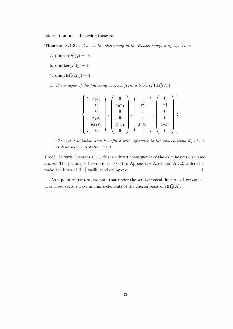
information in the following theorem.
Theorem 3.4.3. Let kn be the chain map of the Koszul complex of Aq. Then
1. dim(Im(k2)2) = 18
2. dim(ker(k3)2) = 14
3. dim(HH22(Aq)) = 4
4. The images of the following cocycles form a basis of HH22(Aq)
x1x3
0
0
x2x3
qx1x4
0
,
0
x2x4
0
0
x1x4
0
,
0
x24
0
0
x3x4
0
,
0
x22
0
0
x2x3
0
The vector notation here is defined with reference to the chosen basis Rq above,
as discussed in Notation 3.2.1.
Proof. As with Theorem 3.3.1, this is a direct consequence of the calculations discussed
above. The particular bases are recorded in Appendices A.2.1 and A.2.2, ordered to
make the basis of HH22 easily read off by eye.
As a point of interest, we note that under the semi-classical limit q → 1 we can see
that these vectors have as limits elements of the chosen basis of HH22(A).
39

40

Chapter 4
A Partial Chain Map from the
Bar Resolution to the Koszul
Resolution for a PBW-Algebra
In this chapter we define a section to the canonical inclusion i∗ : K∗ → B∗ of the Koszul
complex into the bar complex for a PBW algebra. We do this to reduce the generally
difficult problem of calculating Gerstenhaber brackets to a computer calculation. Our
main application of this work will be to calculate which infinitesimal deformations of
A and Aq have vanishing primary obstruction; for a detailed discussion of this please
see Section 5.2.
The work in this chapter is based mostly upon Bergman’s Diamond Lemma [Ber78,
Theorem 2.1] and the theory of reduction systems. Please see Section 2.1.1 for a
discussion of these.
4.1 Preliminaries
Take K to be a field of characteristic 0 and unadorned tensor products to be over K.
We will use both a⊗ b and a|b to represent elements of tensor structures and will freely
interchange between the two.
Recall the definitions from Section 2.1.1 relating to PBW algebras. Throughout this
chapter we assume that A is a PBW algebra generated by a finite set V = {v1, . . . , vγ}.We choose a finite set R ⊆ spK(V )⊗ spK(V ) of relations, so that A = T (V )/(R) with
R chosen so that each relation is of the form
xy −∑
cif1i f
2i where ci ∈ K, x, y, f1
i , f2i ∈ V and f1
i f2i is in PBW order.
Note that since R is homogeneous, A =⊕∞
0 Ai is a graded algebra.
41

Notation 4.1.1. We adopt the notation that for an element v ∈ T (V ) we write[v]
for
v in PBW reduced form with respect to the relations R. Note that[v]
is an element
of T (V ); we write π(v) for the image of v under the canonical projection from T (V ) to
A.
We introduce a dot product on T (V ) for convenience, by extending the following
bilinearly:
(m1 •m2) = δm1,m2 for monomials m1,m2 ∈ T (V ).
Example 4.1.2. We recall the definition of the boundary map of the Koszul complex
in the specific degrees 1,2 and 3 since they will be used extensively throughout this
chapter.
1. The map k1 : A⊗V ⊗A→ A⊗A is defined on the free generating set {1⊗vi⊗1}γi=1
for K1 as :
k1(1⊗ vi ⊗ 1) = π(vi)⊗ 1− 1⊗ π(vi)
2. Let the chosen basis of R be written as {ρσ}σ where each
ρσ = Wσ − fσ = xy −∑i
cif1i f
2i for ci ∈ K∗ and x, y, f ji ∈ V.
Then k2 : A⊗R⊗A→ A⊗ V ⊗A is defined on an element of the generating set
{1⊗ ρσ ⊗ 1}σ as:
k2(1⊗ρσ⊗1) = π(x)⊗y⊗1−∑i
ciπ(f1i
)⊗f2
i ⊗1+1⊗x⊗π(y)−∑i
ci⊗f1i ⊗π
(f2i
)
3. Let a chosen basis of K3 be{∑
i cixi ⊗ ri =∑
j c′j ⊗ r′jzj
}where ci, c
′j ∈ K∗,
ri, r′j ∈ R and xi, zj ∈ V . Then k3 is defined on the corresponding generating set
for K3 as:
k3(1⊗∑i
cixiri ⊗ 1) =∑i
ciπ(xi)⊗ ri ⊗ 1−∑j
c′j ⊗ r′j ⊗ π(zj).
Definition 4.1.3. A partial ordering ≺ on a monoid N is a partial monoid ordering if
for every B,C,M1,M2 ∈ N :
M1 ≺M2 =⇒ BM1C ≺ BM2C.
We write the free monoid on V as 〈V 〉. A partial monoid ordering on 〈V 〉 is said to
be compatible with R if for every σ in the reduction system, each monomial M with
nonzero coefficient in fσ satisfies M ≺Wσ.
42
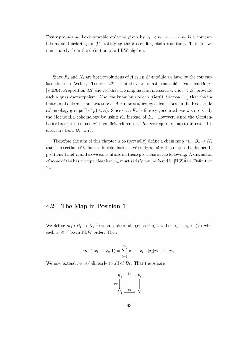
Example 4.1.4. Lexicographic ordering given by v1 ≺ v2 ≺ . . . ≺ vγ is a compat-
ible monoid ordering on 〈V 〉 satisfying the descending chain condition. This follows
immediately from the definition of a PBW-algebra.
Since B∗ and K∗ are both resolutions of A as an Ae-module we have by the compar-
ison theorem [Wei94, Theorem 2.2.6] that they are quasi-isomorphic. Van den Bergh
[VdB94, Proposition 3.3] showed that the map natural inclusion i∗ : K∗ → B∗ provides
such a quasi-isomorphism. Also, we know by work in [Ger64, Section 1.1] that the in-
finitesimal deformation structure of A can be studied by calculations on the Hochschild
cohomology groups Ext∗Ae(A,A). Since each K∗ is finitely generated, we wish to study
the Hochschild cohomology by using K∗ instead of B∗. However, since the Gersten-
haber bracket is defined with explicit reference to B∗, we require a map to transfer this
structure from B∗ to K∗.
Therefore the aim of this chapter is to (partially) define a chain map m∗ : B∗ → K∗
that is a section of i∗ for use in calculations. We only require this map to be defined in
positions 1 and 2, and so we concentrate on those positions in the following. A discussion
of some of the basic properties that m∗ must satisfy can be found in [HSSA14, Definition
1.4].
4.2 The Map in Position 1
We define m1 : B1 → K1 first on a bimodule generating set. Let x1 · · ·xn ∈ 〈V 〉 with
each xi ∈ V be in PBW order. Then
m1(1|x1 · · ·xn|1) =
n∑i=1
x1 · · ·xi−1|xi|xi+1 · · ·xn.
We now extend m1 A-bilinearly to all of B1. That the square
B1 B0
K1 K0
b1
m1
k1
43
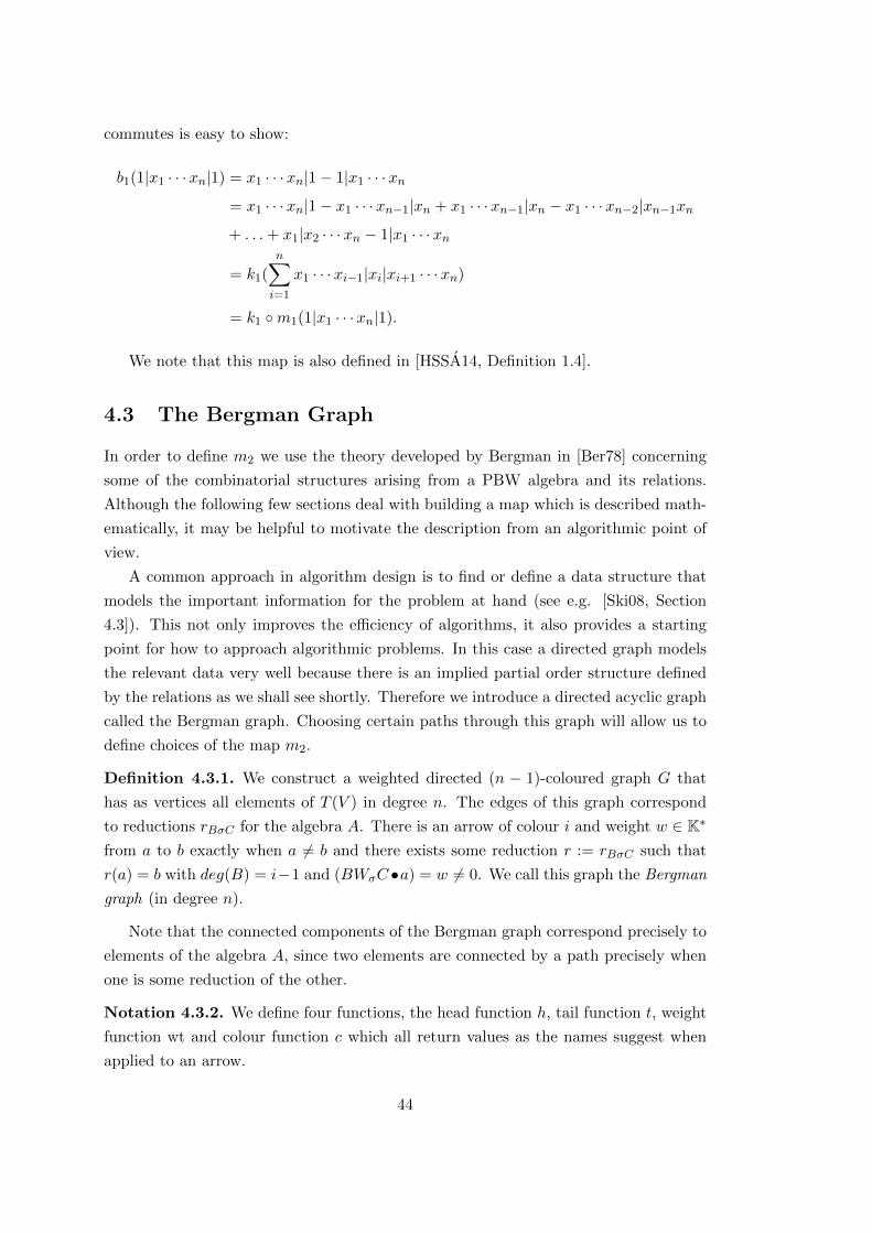
commutes is easy to show:
b1(1|x1 · · ·xn|1) = x1 · · ·xn|1− 1|x1 · · ·xn= x1 · · ·xn|1− x1 · · ·xn−1|xn + x1 · · ·xn−1|xn − x1 · · ·xn−2|xn−1xn
+ . . .+ x1|x2 · · ·xn − 1|x1 · · ·xn
= k1(n∑i=1
x1 · · ·xi−1|xi|xi+1 · · ·xn)
= k1 ◦m1(1|x1 · · ·xn|1).
We note that this map is also defined in [HSSA14, Definition 1.4].
4.3 The Bergman Graph
In order to define m2 we use the theory developed by Bergman in [Ber78] concerning
some of the combinatorial structures arising from a PBW algebra and its relations.
Although the following few sections deal with building a map which is described math-
ematically, it may be helpful to motivate the description from an algorithmic point of
view.
A common approach in algorithm design is to find or define a data structure that
models the important information for the problem at hand (see e.g. [Ski08, Section
4.3]). This not only improves the efficiency of algorithms, it also provides a starting
point for how to approach algorithmic problems. In this case a directed graph models
the relevant data very well because there is an implied partial order structure defined
by the relations as we shall see shortly. Therefore we introduce a directed acyclic graph
called the Bergman graph. Choosing certain paths through this graph will allow us to
define choices of the map m2.
Definition 4.3.1. We construct a weighted directed (n − 1)-coloured graph G that
has as vertices all elements of T (V ) in degree n. The edges of this graph correspond
to reductions rBσC for the algebra A. There is an arrow of colour i and weight w ∈ K∗
from a to b exactly when a 6= b and there exists some reduction r := rBσC such that
r(a) = b with deg(B) = i−1 and (BWσC •a) = w 6= 0. We call this graph the Bergman
graph (in degree n).
Note that the connected components of the Bergman graph correspond precisely to
elements of the algebra A, since two elements are connected by a path precisely when
one is some reduction of the other.
Notation 4.3.2. We define four functions, the head function h, tail function t, weight
function wt and colour function c which all return values as the names suggest when
applied to an arrow.
44
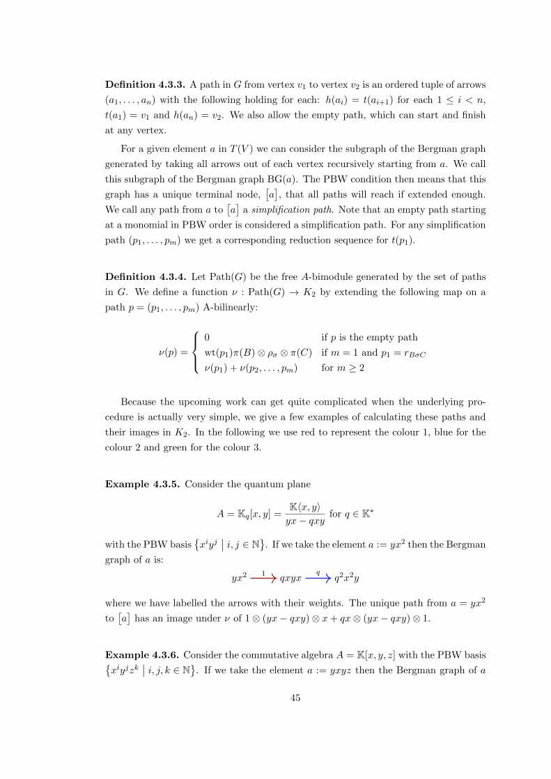
Definition 4.3.3. A path in G from vertex v1 to vertex v2 is an ordered tuple of arrows
(a1, . . . , an) with the following holding for each: h(ai) = t(ai+1) for each 1 ≤ i < n,
t(a1) = v1 and h(an) = v2. We also allow the empty path, which can start and finish
at any vertex.
For a given element a in T (V ) we can consider the subgraph of the Bergman graph
generated by taking all arrows out of each vertex recursively starting from a. We call
this subgraph of the Bergman graph BG(a). The PBW condition then means that this
graph has a unique terminal node,[a], that all paths will reach if extended enough.
We call any path from a to[a]
a simplification path. Note that an empty path starting
at a monomial in PBW order is considered a simplification path. For any simplification
path (p1, . . . , pm) we get a corresponding reduction sequence for t(p1).
Definition 4.3.4. Let Path(G) be the free A-bimodule generated by the set of paths
in G. We define a function ν : Path(G) → K2 by extending the following map on a
path p = (p1, . . . , pm) A-bilinearly:
ν(p) =
0 if p is the empty path
wt(p1)π(B)⊗ ρσ ⊗ π(C) if m = 1 and p1 = rBσC
ν(p1) + ν(p2, . . . , pm) for m ≥ 2
Because the upcoming work can get quite complicated when the underlying pro-
cedure is actually very simple, we give a few examples of calculating these paths and
their images in K2. In the following we use red to represent the colour 1, blue for the
colour 2 and green for the colour 3.
Example 4.3.5. Consider the quantum plane
A = Kq[x, y] =K〈x, y〉yx− qxy
for q ∈ K∗
with the PBW basis{xiyj
∣∣ i, j ∈ N}
. If we take the element a := yx2 then the Bergman
graph of a is:
yx2 qxyx q2x2y1 q
where we have labelled the arrows with their weights. The unique path from a = yx2
to[a]
has an image under ν of 1⊗ (yx− qxy)⊗ x+ qx⊗ (yx− qxy)⊗ 1.
Example 4.3.6. Consider the commutative algebra A = K[x, y, z] with the PBW basis{xiyjzk
∣∣ i, j, k ∈ N}
. If we take the element a := yxyz then the Bergman graph of a
45

is:yxyz
yzxy yxzy xy2z
xyzy
where all of the weights are 1 in this case. Let p be the top path and q be the bottom
path. Then:
ν(p) = ν(q) = y ⊗ [z, x]⊗ y + yx⊗ [z, y]⊗ 1 + 1⊗ [y, x]⊗ yz.
The fact that these two paths have the same image under ν is no accident and is
an example of a somewhat subtle phenomenon which will be investigated below.
Example 4.3.7. Consider the Jordan plane:
A =K〈x, y〉
(yx− xy − y2)
with the PBW basis{xiyj
∣∣ i, j ∈ N}
. Set r := xy − yx− y2 ∈ V ⊗ V .
If we take the element a := yx2 then the Bergman graph of a is:
x2y + xy2 + y2x
yx2 xyx+ y2x x2y + xy2 + yxy + y3
xyx+ yxy + y3 x2y + 2xy2 + 2y3
xyx+ xy2 + 2y3
where all of the weights are 1 in this case. The three different choices of path all have
the same image under ν, which is
1⊗ r ⊗ x+ x⊗ r ⊗ 1 + y ⊗ r ⊗ 1 + 1⊗ r ⊗ y.
4.4 The Minimal Partial Monoid Order on 〈V 〉
In this section we show that the definition of a compatible monoid order actually
suffices to define a compatible monoid order that is the minimal partial order with that
property. This minimal ordering provides a very useful tool for reasoning about paths
in the Bergman graph because, as we shall prove, a monomial x is related to another
46
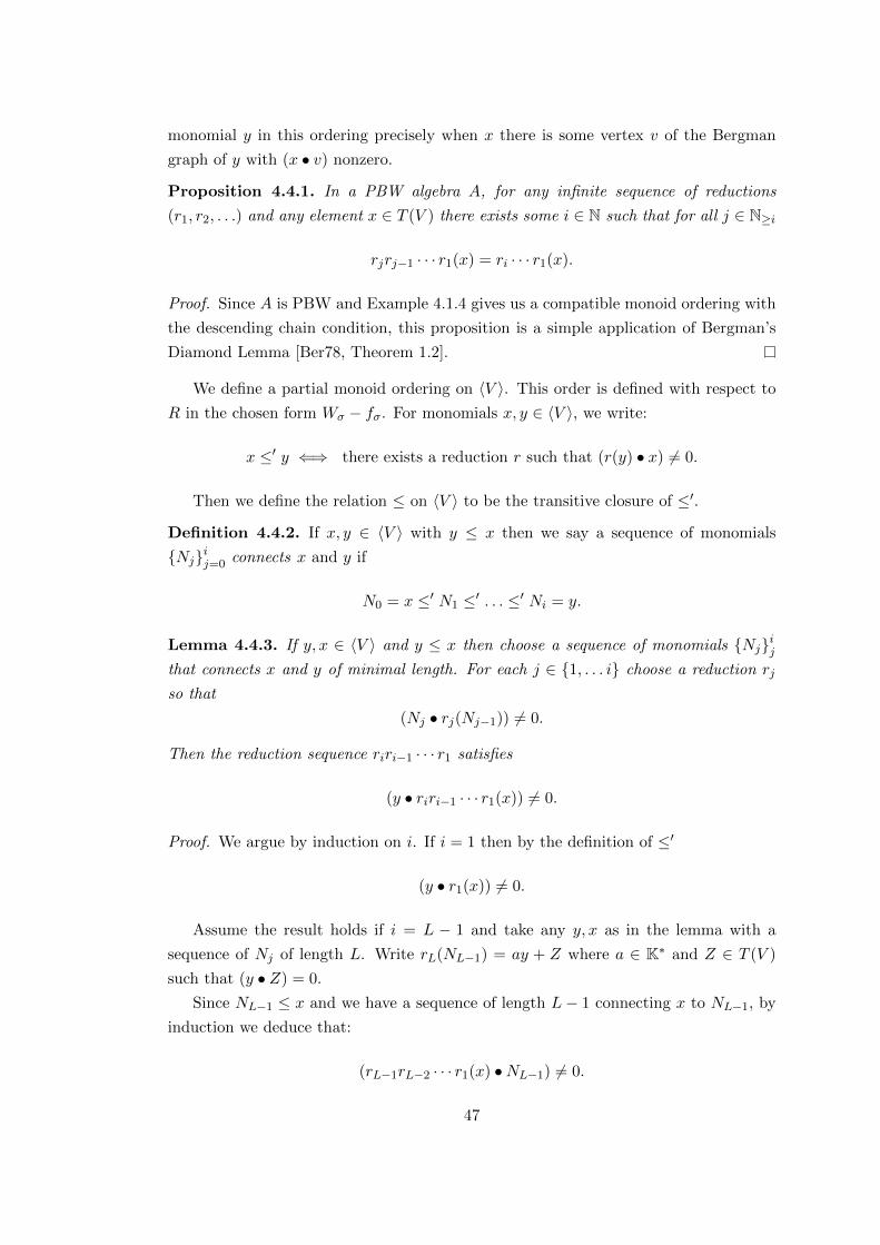
monomial y in this ordering precisely when x there is some vertex v of the Bergman
graph of y with (x • v) nonzero.
Proposition 4.4.1. In a PBW algebra A, for any infinite sequence of reductions
(r1, r2, . . .) and any element x ∈ T (V ) there exists some i ∈ N such that for all j ∈ N≥i
rjrj−1 · · · r1(x) = ri · · · r1(x).
Proof. Since A is PBW and Example 4.1.4 gives us a compatible monoid ordering with
the descending chain condition, this proposition is a simple application of Bergman’s
Diamond Lemma [Ber78, Theorem 1.2].
We define a partial monoid ordering on 〈V 〉. This order is defined with respect to
R in the chosen form Wσ − fσ. For monomials x, y ∈ 〈V 〉, we write:
x ≤′ y ⇐⇒ there exists a reduction r such that (r(y) • x) 6= 0.
Then we define the relation ≤ on 〈V 〉 to be the transitive closure of ≤′.
Definition 4.4.2. If x, y ∈ 〈V 〉 with y ≤ x then we say a sequence of monomials
{Nj}ij=0 connects x and y if
N0 = x ≤′ N1 ≤′ . . . ≤′ Ni = y.
Lemma 4.4.3. If y, x ∈ 〈V 〉 and y ≤ x then choose a sequence of monomials {Nj}ijthat connects x and y of minimal length. For each j ∈ {1, . . . i} choose a reduction rj
so that
(Nj • rj(Nj−1)) 6= 0.
Then the reduction sequence riri−1 · · · r1 satisfies
(y • riri−1 · · · r1(x)) 6= 0.
Proof. We argue by induction on i. If i = 1 then by the definition of ≤′
(y • r1(x)) 6= 0.
Assume the result holds if i = L − 1 and take any y, x as in the lemma with a
sequence of Nj of length L. Write rL(NL−1) = ay + Z where a ∈ K∗ and Z ∈ T (V )
such that (y • Z) = 0.
Since NL−1 ≤ x and we have a sequence of length L− 1 connecting x to NL−1, by
induction we deduce that:
(rL−1rL−2 · · · r1(x) •NL−1) 6= 0.
47
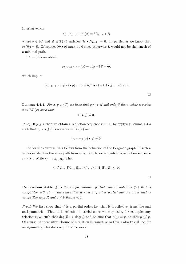
In other words
rL−1rL−2 · · · r1(x) = bNL−1 + Θ
where b ∈ K∗ and Θ ∈ T (V ) satisfies (Θ • NL−1) = 0. In particular we know that
rL(Θ) = Θ. Of course, (Θ • y) must be 0 since otherwise L would not be the length of
a minimal path.
From this we obtain
rLrL−1 · · · r1(x) = aby + bZ + Θ,
which implies
(rLrL−1 · · · r1(x) • y) = ab+ b(Z • y) + (Θ • y) = ab 6= 0.
Lemma 4.4.4. For x, y ∈ 〈V 〉 we have that y ≤ x if and only if there exists a vertex
v in BG(x) such that
(v • y) 6= 0.
Proof. If y ≤ x then we obtain a reduction sequence ri · · · r1 by applying Lemma 4.4.3
such that ri · · · r1(x) is a vertex in BG(x) and
(ri · · · r1(x) • y) 6= 0.
As for the converse, this follows from the definition of the Bergman graph. If such a
vertex exists then there is a path from x to v which corresponds to a reduction sequence
ri · · · r1. Write rj = rAjσjBj . Then
y ≤′ Ai−1Wσi−1Bi−1 ≤′ . . . ≤′ A1Wσ1B1 ≤′ x.
Proposition 4.4.5. ≤ is the unique minimal partial monoid order on 〈V 〉 that is
compatible with R, in the sense that if ≺ is any other partial monoid order that is
compatible with R and a ≤ b then a ≺ b.
Proof. We first show that ≤ is a partial order, i.e. that it is reflexive, transitive and
antisymmetric. That ≤ is reflexive is trivial since we may take, for example, any
relation rBσC such that deg(B) > deg(y) and be sure that r(y) = y, so that y ≤′ y.
Of course, the transitive closure of a relation is transitive so this is also trivial. As for
antisymmetry, this does require some work.
48

If x, y ∈ 〈V 〉 with x ≤ y and y ≤ x then we prove by contradiction that x = y. If
x 6= y then take a sequence M1, . . .Mj−1 ∈ 〈V 〉 of minimal length such that
x ≤′ Mj−1 . . . ≤′ M1 ≤′ y
and likewise a sequence N1 . . . Ni−1 ∈ 〈V 〉 of minimal length connecting y to x:
y ≤′ Ni−1 ≤′ . . . ≤′ N1 ≤′ x.
We induct on i+ j.
Base Case: If x ≤′ y and y ≤′ x then there are two reductions s, r such that s(y) = bx + B
and r(x) = cy + C where
(B • x) = (B • y) = (C • x) = (C • y) = 0.
Now we claim that (r, s, r, s, . . .) is an infinite sequence of reductions that never
stabilises when applied to x. Note that
sr(x) = bcx+ cB + C.
Therefore if d, e ∈ K satisfy:
(sr)n(x) = bicjx+ dB + eC,
then
r(sr)n(x) = bicj+1y + (bicj + e)C + dB
and
(sr)n+1(x) = bi+1cj+1x+ (bicj + e)C + (bicj+1 + d)B,
since B and C are orthogonal to both x and y. Therefore (r, s, r, s, r . . .) never
stabilises when applied to x. This contradicts Proposition 4.4.1.
Inductive case: We reduce to the case that j = 1 by noting that x ≤′ Mj−1 by definition and
Mj−1 ≤ x is given by considering the sequence Mj−2, . . . ,M1, y,Ni−1, . . . , N1. If
there is a shorter sequence connecting Mj−1 and x then by induction Mj−1 = x
and the original sequences were not minimal. Therefore we may pass to the case
that x ≤′ y and y ≤′ Ni−1 ≤′ . . . ≤′ N1 ≤′ x.
By Lemma 4.4.3 we obtain a reduction sequence riri−1 · · · r1 such that
riri−1 · · · r1(x) = by +B for some b ∈ K∗ and B ∈ T (V ) satisfying (B • y) = 0.
49

We claim that furthermore (B •Nl) = 0 for all l. Indeed if there is some Nl for
which (Nl •B) 6= 0 then consider that there must be a smallest m > l such that
(rm+1rm · · · rl · · · r1(x) •Nl) 6= 0
which by definition would imply that (rm(Nm) •Nl) 6= 0 and so Nm ≤′ Nl.
But Nm ≤ Nl by definition, and so we have Nl = Nm by induction, contradicting
the minimality of i.
By the same argument, if s is a reduction such that s(y) = cx + C with c ∈ K∗
and C orthogonal to both of x and y, then
(Nj • C) = 0 for all j.
Therefore (r1, . . . , rn, s, . . .) forms an infinite sequence of reductions that never
stabilises when applied to x, since it must always pass through elements of the
form:
dx+ eB + fC and gy + hB + iC for some e, f, h, i ∈ K and d, g ∈ K∗.
This contradicts Proposition 4.4.1 and provides the inductive step.
Therefore ≤ is a partial order on 〈V 〉. That it is also a monoid order is trivial since for
any M,N ∈ 〈V 〉
rCσD(y) = ax+ Z for a ∈ K∗ and Z ∈ T (V ) orthogonal to x and y
implies
(rMCσDN (MyN) •MxN) = (M(ax+ Z)N •MxN) = a 6= 0.
That minimal orders are unique is obvious, and that ≤ is minimal is clear since the
definition of compatible is that if r(y) = bx + B for some r then x ≺ y. Since any
partial order must be transitive, then x ≤ y implies that x ≺ y.
As a simple corollary to Proposition 4.4.5 and Lemma 4.4.4, the Bergman graph
is a directed acyclic graph. Since there are a finite number of monomials of any given
degree, and the relations of A are homogeneous, we also know that ≤ satisfies the
descending chain condition. We also record the following useful fact.
Lemma 4.4.6. There is an upper limit for the length of a path in BG(a) that depends
only upon a ∈ T (V ).
50

Proof. Call this limit U(a). We make an induction argument. If a is in PBW order
then this limit is zero. Otherwise, assume the result holds for all b such that there is a
reduction r with r(a) = b. Then the upper limit for a is
max {U(b) | a→r b}+ 1.
4.5 A Few Operations on Paths
We define some useful operations on edges in the Bergman graph. Since the Bergman
graph has vertices that are elements of T (V ), there is an obvious T (V )-bimodule struc-
ture on the free group of vertices. We shall see below that this defines a T (V )-bimodule
structure on the free group of edges as well and that ν ‘respects’ this structure in a
useful way.
Furthermore, one would expect there to be some relationship between BG(a) and
BG(a + X) for some a,X ∈ T (V ). Although a full description of this relationship
would be cumbersome (and unhelpful), we note a particular case in which BG(a) is a
subgraph of BG(a + X) and this fact is very useful in reasoning about paths in the
Bergman graph.
Definition 4.5.1. Let X ∈ T (V ) and a ∈ 〈V 〉. If for every v ∈ 〈V 〉 \ {a} such that
(X • v) 6= 0 we have that v ≤ a implies that v =[v], then we say X doesn’t interfere
with a. In other words, if X =∑
i cimi for constants ci ∈ K∗ and monomials mi ∈ 〈V 〉,then either mi =
[mi
]or mi 6≤ a.
Otherwise, we say X interferes with a.
Note that non-interference is an inheritable property in the sense that if m ≤ a and
X ∈ T (V ) doesn’t interfere with a then X doesn’t interfere with m.
Definition 4.5.2. If p is a path in the Bergman graph starting from a ∈ 〈V 〉, and
X ∈ T (V ) doesn’t interfere with a, then we define the translation of p by X, written
pX , to be the path corresponding to the same reductions as p starting from a+X.
Lemma 4.5.3. 1. If x ≤ y then there exists a vertex v in BG(y) such that
v = ax+X
where a ∈ K∗ and X ∈ T (V ) doesn’t interfere with x.
2. If x ≤ y then BG(x) is isomorphic to a subgraph of BG(y) rooted at any vertex
ax+X in BG(y) where a ∈ K∗ and X ∈ T (V ) doesn’t interfere with x.
51

Proof. 1. Since x ≤ y then by Proposition 4.4.5 there is a vertex v in BG(y) such
that
v = ax+ Z
where Z is orthogonal to x and a ∈ K∗. However, it is possible that Z does
interfere with x. With that in mind we decompose Z as
Z = Z1 + Z2
where Z1, Z2 ∈ T (V ). We choose Z2 so that it doesn’t interfere with x and every
monomial m such that (m • Z1) 6= 0 satisfies m < x and m is out of PBW order.
In this way Z1 contains all of the ‘interfering’ monomials in Z.
Then there is another vertex in BG(y)
v′ = ax+[Z1
]+ Z2
with[Z1
]orthogonal to x. Then X :=
[Z1
]+ Z2 doesn’t interfere with x.
2. Since X doesn’t interfere with x, we obtain an injective mapping BG(x) ↪→ BG(y)
defined by taking an edge e to eX .
Definition 4.5.4. If y ∈ 〈V 〉 and p is a path∑xi
w1−−−−−→rB1σ1C1
. . .wn−−−−−−→
rBnσnCn
∑zi
then we define the right stitch of p by y to be the path:∑xiy
w1−−−−−−−→rB1σ1(C1y)
. . .wn−−−−−−−→
rBnσn(Cny)
∑ziy.
We write this path as p 999y. The left stitch y 999p is defined analogously:
∑yxi
w1−−−−−−−→r(yB1)σ1C1
. . .wn−−−−−−→
r(yBn)σnC
∑yzi.
Remark 4.5.5. Although we will not use the full structure here, stitching provides a
T (V )-bimodule structure on the additive free group of paths in the Bergman graph.
Lemma 4.5.6. 1. For a path p and y ∈ 〈V 〉 the following holds:
ν(p 999y) = ν(p)π(y).
Likewise:
ν(y 999p) = π(y) ν(p).
52
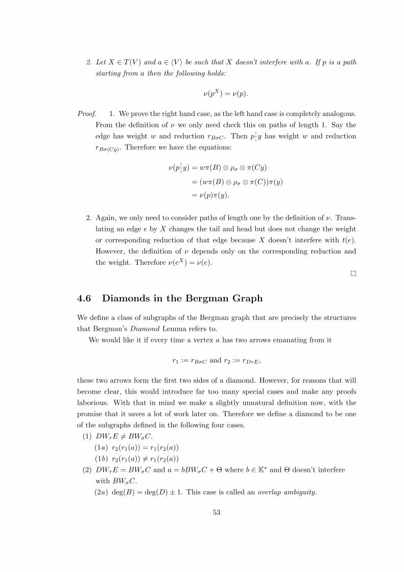
2. Let X ∈ T (V ) and a ∈ 〈V 〉 be such that X doesn’t interfere with a. If p is a path
starting from a then the following holds:
ν(pX) = ν(p).
Proof. 1. We prove the right hand case, as the left hand case is completely analogous.
From the definition of ν we only need check this on paths of length 1. Say the
edge has weight w and reduction rBσC . Then p 999y has weight w and reduction
rBσ(Cy). Therefore we have the equations:
ν(p 999y) = wπ(B)⊗ ρσ ⊗ π(Cy)
= (wπ(B)⊗ ρσ ⊗ π(C))π(y)
= ν(p)π(y).
2. Again, we only need to consider paths of length one by the definition of ν. Trans-
lating an edge e by X changes the tail and head but does not change the weight
or corresponding reduction of that edge because X doesn’t interfere with t(e).
However, the definition of ν depends only on the corresponding reduction and
the weight. Therefore ν(eX) = ν(e).
4.6 Diamonds in the Bergman Graph
We define a class of subgraphs of the Bergman graph that are precisely the structures
that Bergman’s Diamond Lemma refers to.
We would like it if every time a vertex a has two arrows emanating from it
r1 := rBσC and r2 := rDτE ,
these two arrows form the first two sides of a diamond. However, for reasons that will
become clear, this would introduce far too many special cases and make any proofs
laborious. With that in mind we make a slightly unnatural definition now, with the
promise that it saves a lot of work later on. Therefore we define a diamond to be one
of the subgraphs defined in the following four cases.
(1) DWτE 6= BWσC.
(1a) r2(r1(a)) = r1(r2(a))
(1b) r2(r1(a)) 6= r1(r2(a))
(2) DWτE = BWσC and a = bBWσC + Θ where b ∈ K∗ and Θ doesn’t interfere
with BWσC.
(2a) deg(B) = deg(D)± 1. This case is called an overlap ambiguity .
53

(2b) deg(B) 6= deg(D)± 1.
We describe the subgraph that forms the diamond in each case.
(1) In both of these cases, a = bBWσC+ cDWτE+ Θ where Θ is orthogonal to both
BWσC and DWτE and b, c ∈ K∗. Let m1 = BWσC and m2 = DWτE. Since
m1,m2 ∈ 〈V 〉 and m1 6= m2, we know (m1 •m2) = 0.
(1a) The subgraph is precisely that formed by the edges corresponding to r1 and r2 in
the equality: r2(r1(a)) = r1(r2(a)). That is the subgraph:
r1
r2 r1
r2bBWσC + cDWτE + Θ
bBWσC + cDfτE + Θ.
bBfσC + cDWτE + Θ
bBfσC + cDfτE + Θ
(1b) Since r2(r1(a)) 6= r1(r2(a)), we claim that either m2 ≤′ m1 or m1 ≤′ m2 (but
not both since m1 6= m2). Assume neither inequality holds for a contradiction.
Then as in the previous case r1(a) = br1(m1) + cm2 + Θ, and since m2 6≤′ m1, we
know that r2(r1(a)) = br1(m1) + cr2(m2) + Θ. But by symmetry we have that
r1(r2(a)) = br1(m1) + cr2(m2) + Θ = r2(r1(a)), which contradicts the definition
of case (1b).
Then without loss of generality we may assume m2 ≤′ m1. Let r1(m1) = dm2+Z,
where Z is orthogonal to both m1 and m2, and d ∈ K∗. Then the following holds:
r2(r1(a)) = r2(r1(bm1 + cm2 + Θ))
= r2(bdm2 + bZ + cm2 + Θ)
= (bd+ c)r2(m2) + bZ + Θ.
Alternatively, we also have:
r2(r1(r2(a))) = r2(r1(r2(bm1 + cm2 + Θ)))
= r2(r1(bm1 + cr2(m2) + Θ))
= r2(bdm2 + bZ + cr2(m2) + Θ) since m1 6≤′ m2
= (bd+ c)r2(m2) + bZ + Θ = r2(r1(a)).
The diamond is the subgraph corresponding to this identity:
54
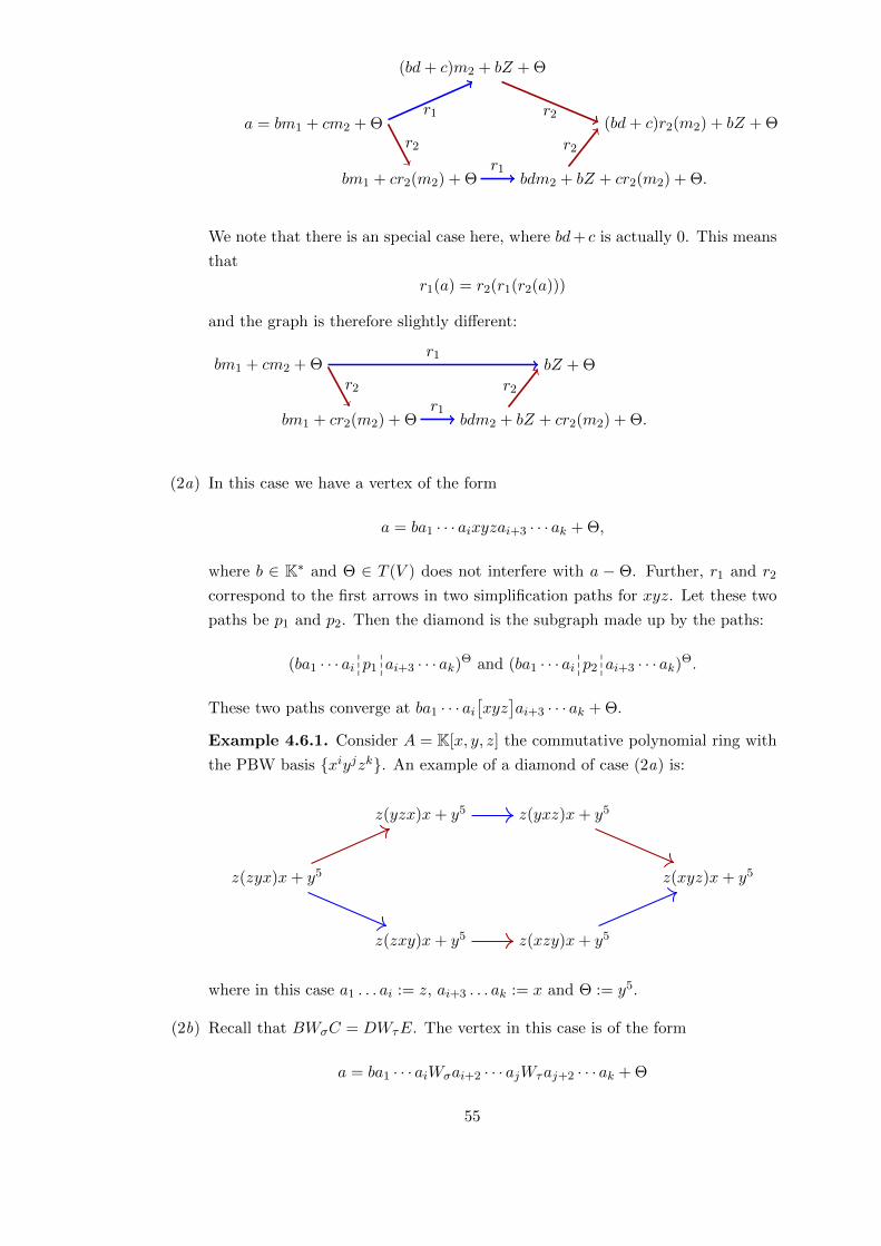
r1
r2
r1
r2
r2
a = bm1 + cm2 + Θ
bm1 + cr2(m2) + Θ bdm2 + bZ + cr2(m2) + Θ.
(bd+ c)m2 + bZ + Θ
(bd+ c)r2(m2) + bZ + Θ
We note that there is an special case here, where bd+ c is actually 0. This means
that
r1(a) = r2(r1(r2(a)))
and the graph is therefore slightly different:
r1
r2
r1
r2
bm1 + cm2 + Θ
bm1 + cr2(m2) + Θ bdm2 + bZ + cr2(m2) + Θ.
bZ + Θ
(2a) In this case we have a vertex of the form
a = ba1 · · · aixyzai+3 · · · ak + Θ,
where b ∈ K∗ and Θ ∈ T (V ) does not interfere with a − Θ. Further, r1 and r2
correspond to the first arrows in two simplification paths for xyz. Let these two
paths be p1 and p2. Then the diamond is the subgraph made up by the paths:
(ba1 · · · ai 999p1 999ai+3 · · · ak)Θ and (ba1 · · · ai 999p2 999ai+3 · · · ak)Θ.
These two paths converge at ba1 · · · ai[xyz
]ai+3 · · · ak + Θ.
Example 4.6.1. Consider A = K[x, y, z] the commutative polynomial ring with
the PBW basis {xiyjzk}. An example of a diamond of case (2a) is:
z(yzx)x+ y5 z(yxz)x+ y5
z(zyx)x+ y5 z(xyz)x+ y5
z(zxy)x+ y5 z(xzy)x+ y5
where in this case a1 . . . ai := z, ai+3 . . . ak := x and Θ := y5.
(2b) Recall that BWσC = DWτE. The vertex in this case is of the form
a = ba1 · · · aiWσai+2 · · · ajWτaj+2 · · · ak + Θ
55
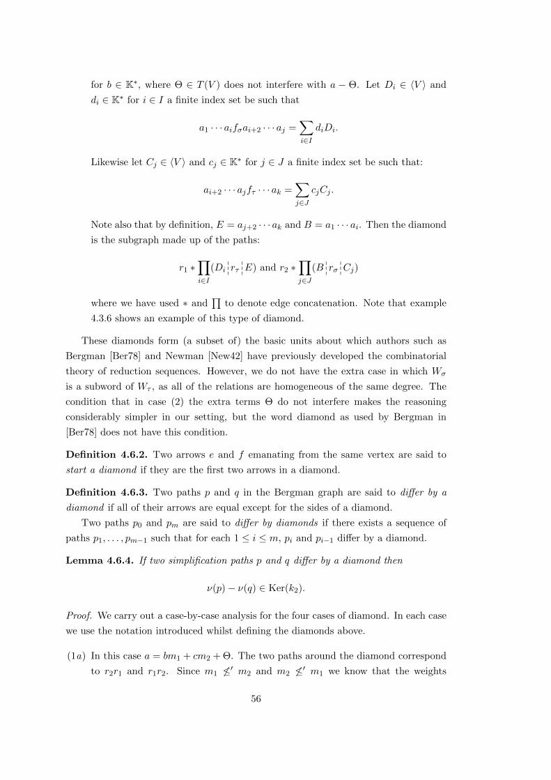
for b ∈ K∗, where Θ ∈ T (V ) does not interfere with a − Θ. Let Di ∈ 〈V 〉 and
di ∈ K∗ for i ∈ I a finite index set be such that
a1 · · · aifσai+2 · · · aj =∑i∈I
diDi.
Likewise let Cj ∈ 〈V 〉 and cj ∈ K∗ for j ∈ J a finite index set be such that:
ai+2 · · · ajfτ · · · ak =∑j∈J
cjCj .
Note also that by definition, E = aj+2 · · · ak and B = a1 · · · ai. Then the diamond
is the subgraph made up of the paths:
r1 ∗∏i∈I
(Di 999rτ 999E) and r2 ∗
∏j∈J
(B 999rσ 999Cj)
where we have used ∗ and∏
to denote edge concatenation. Note that example
4.3.6 shows an example of this type of diamond.
These diamonds form (a subset of) the basic units about which authors such as
Bergman [Ber78] and Newman [New42] have previously developed the combinatorial
theory of reduction sequences. However, we do not have the extra case in which Wσ
is a subword of Wτ , as all of the relations are homogeneous of the same degree. The
condition that in case (2) the extra terms Θ do not interfere makes the reasoning
considerably simpler in our setting, but the word diamond as used by Bergman in
[Ber78] does not have this condition.
Definition 4.6.2. Two arrows e and f emanating from the same vertex are said to
start a diamond if they are the first two arrows in a diamond.
Definition 4.6.3. Two paths p and q in the Bergman graph are said to differ by a
diamond if all of their arrows are equal except for the sides of a diamond.
Two paths p0 and pm are said to differ by diamonds if there exists a sequence of
paths p1, . . . , pm−1 such that for each 1 ≤ i ≤ m, pi and pi−1 differ by a diamond.
Lemma 4.6.4. If two simplification paths p and q differ by a diamond then
ν(p)− ν(q) ∈ Ker(k2).
Proof. We carry out a case-by-case analysis for the four cases of diamond. In each case
we use the notation introduced whilst defining the diamonds above.
(1a) In this case a = bm1 + cm2 + Θ. The two paths around the diamond correspond
to r2r1 and r1r2. Since m1 6≤′ m2 and m2 6≤′ m1 we know that the weights
56

associated with both edges corresponding to r1 are the same, and likewise for
those corresponding to r2. That is:
ν(p)− ν(q) = (bB ⊗ ρσ ⊗C + cD ⊗ ρτ ⊗E)− (cD ⊗ ρτ ⊗E + bB ⊗ ρτ ⊗E) = 0.
(1b) We have that a = bm1 + cm2 + Θ. Recall that we also let r1(m1) = dm2 +Z. We
show that ν(p− q) = 0 in either the general case or the case where bd+ c = 0.
In the general case recall that:
r2(r1(r2(a))) = (bd+ c)r2(m2) + bZ + Θ = r2(r1(a)),
corresponding to the graph:
r1
r2
r1
r2
r2
a = bm1 + cm2 + Θ
bm1 + cr2(m2) + Θ bdm2 + bZ + cr2(m2) + Θ.
(bd+ c)m2 + bZ + Θ
(bd+ c)r2(m2) + bZ + Θ
Recall that m1 = BWσC and m2 = DWτE. Now, if we set p and q to be the
bottom and top paths respectively we have that
ν(p) = c(D ⊗ ρτ ⊗ E) + b(B ⊗ ρσ ⊗ C) + bd(D ⊗ ρτ ⊗ E)
= b(B ⊗ ρσ ⊗ C) + (bd+ c)(D ⊗ ρτ ⊗ E)
= ν(q).
In the case where bd+ c = 0, then r2(r1(r2(a))) = r1(a) and
ν(p) = c(D ⊗ ρτ ⊗ E) + b(B ⊗ ρσ ⊗ C) + bd(D ⊗ ρτ ⊗ E)
= b(B ⊗ ρσ ⊗ C)
= ν(q).
(2a) Recall that we write[Z]
for the PBW reduced form of an element Z ∈ T (V ). We
show that overlap ambiguities actually correspond to elements of K3. Observe
that the definition of the diamond in this case is a translation of a stitch of two
simplification paths for xyz. By Lemma 4.5.6, the difference ν(p− q) is the same
as the image under ν of the difference of these two simplification paths.
Thus it suffices to consider the following situation, where a red corresponds to
57

the colour 0, blue corresponds with the colour 1 and a coloured dashed arrow
corresponds to zero or more arrows with the first one being the colour shown.
xyz[xyz
]
Let p be the top path and q be the bottom path. By the definition of a path, if
we take the sum∑
e(t(e)− h(e)) over edges e in a path, we obtain an expression
equal to the beginning of the path minus the end. Applying this to p and q we
obtain two ways of writing the expression xyz −[xyz
]. For p we obtain:∑
cixiri +∑
c′jr′jx′j = xyz −
[xyz
], (†)
where the ci, c′i ∈ K∗ and the ri, r
′i are relations. Since p is of length at least one,
there is some c′j that is nonzero. By symmetry we get another expression for the
bottom path: ∑diyisi +
∑d′js′jy′j = xyz −
[xyz
], (††)
where there is at least one di nonzero, all the di, d′j ∈ K∗ and si, s
′j are relations.
Taking the difference of the right hand sides of (†) and (††), we get 0 = xyz −[xyz
]− (xyz−
[xyz
]). However, by grouping together like terms in the difference
of the left hand sides we get an expression of the form:
0 =∑j
ejzjtj −∑i
e′it′iz′i ∈ T (V ),
with both of the sums being nonzero, and the ei’s and e′i’s nonzero scalars. This
implies that ∑j
ej |zj |tj |1 =∑i
e′i|t′i|z′i|1 ∈ K3
and so
ν(p− q) =∑i
e′i|t′i|z′i −∑j
ejzj |tj |1 = k3(∑
ej |zj |tj |1)
by the definition of k3. Therefore k2(ν(p− q)) = 0.
(2b) To start we consider the case of a monomial of the form
a1 · · · aiWσai+2 · · · ajWτaj+2 · · · ak.
The graph in question will have the following appearance:
58
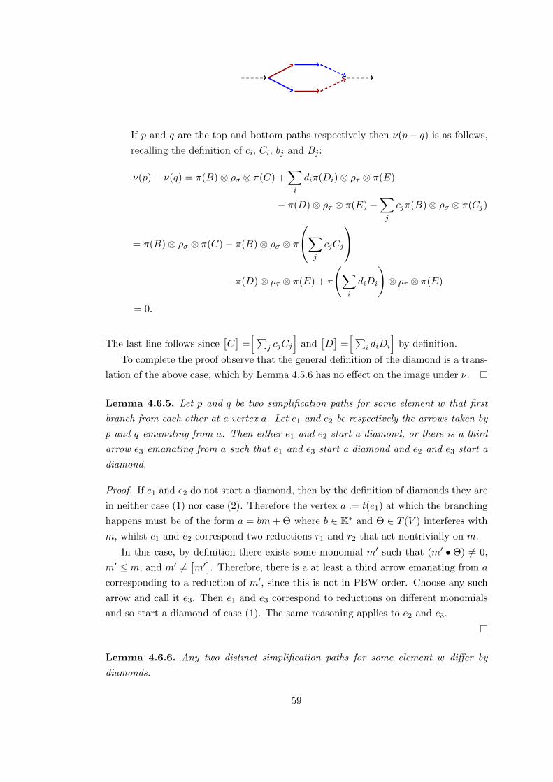
If p and q are the top and bottom paths respectively then ν(p− q) is as follows,
recalling the definition of ci, Ci, bj and Bj :
ν(p)− ν(q) = π(B)⊗ ρσ ⊗ π(C) +∑i
diπ(Di)⊗ ρτ ⊗ π(E)
− π(D)⊗ ρτ ⊗ π(E)−∑j
cjπ(B)⊗ ρσ ⊗ π(Cj)
= π(B)⊗ ρσ ⊗ π(C)− π(B)⊗ ρσ ⊗ π
∑j
cjCj
− π(D)⊗ ρτ ⊗ π(E) + π
(∑i
diDi
)⊗ ρτ ⊗ π(E)
= 0.
The last line follows since[C]
=[∑
j cjCj
]and
[D]
=[∑
i diDi
]by definition.
To complete the proof observe that the general definition of the diamond is a trans-
lation of the above case, which by Lemma 4.5.6 has no effect on the image under ν.
Lemma 4.6.5. Let p and q be two simplification paths for some element w that first
branch from each other at a vertex a. Let e1 and e2 be respectively the arrows taken by
p and q emanating from a. Then either e1 and e2 start a diamond, or there is a third
arrow e3 emanating from a such that e1 and e3 start a diamond and e2 and e3 start a
diamond.
Proof. If e1 and e2 do not start a diamond, then by the definition of diamonds they are
in neither case (1) nor case (2). Therefore the vertex a := t(e1) at which the branching
happens must be of the form a = bm+ Θ where b ∈ K∗ and Θ ∈ T (V ) interferes with
m, whilst e1 and e2 correspond two reductions r1 and r2 that act nontrivially on m.
In this case, by definition there exists some monomial m′ such that (m′ • Θ) 6= 0,
m′ ≤ m, and m′ 6=[m′]. Therefore, there is a at least a third arrow emanating from a
corresponding to a reduction of m′, since this is not in PBW order. Choose any such
arrow and call it e3. Then e1 and e3 correspond to reductions on different monomials
and so start a diamond of case (1). The same reasoning applies to e2 and e3.
Lemma 4.6.6. Any two distinct simplification paths for some element w differ by
diamonds.
59
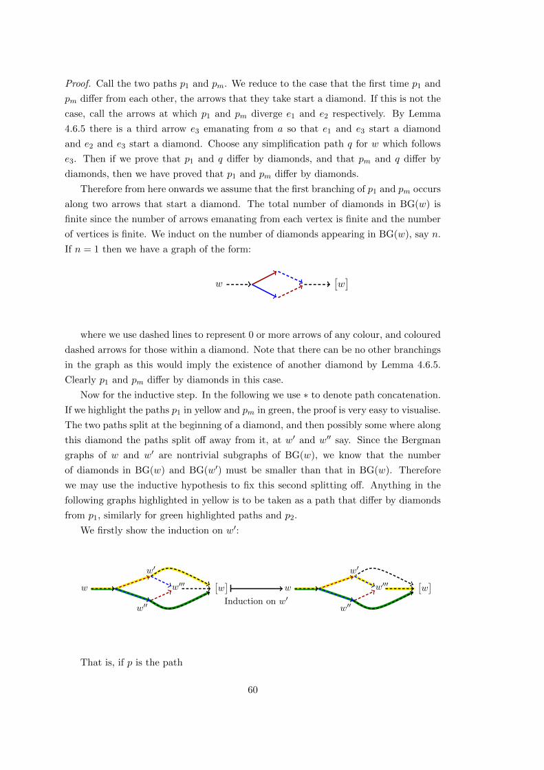
Proof. Call the two paths p1 and pm. We reduce to the case that the first time p1 and
pm differ from each other, the arrows that they take start a diamond. If this is not the
case, call the arrows at which p1 and pm diverge e1 and e2 respectively. By Lemma
4.6.5 there is a third arrow e3 emanating from a so that e1 and e3 start a diamond
and e2 and e3 start a diamond. Choose any simplification path q for w which follows
e3. Then if we prove that p1 and q differ by diamonds, and that pm and q differ by
diamonds, then we have proved that p1 and pm differ by diamonds.
Therefore from here onwards we assume that the first branching of p1 and pm occurs
along two arrows that start a diamond. The total number of diamonds in BG(w) is
finite since the number of arrows emanating from each vertex is finite and the number
of vertices is finite. We induct on the number of diamonds appearing in BG(w), say n.
If n = 1 then we have a graph of the form:
w[w]
where we use dashed lines to represent 0 or more arrows of any colour, and coloured
dashed arrows for those within a diamond. Note that there can be no other branchings
in the graph as this would imply the existence of another diamond by Lemma 4.6.5.
Clearly p1 and pm differ by diamonds in this case.
Now for the inductive step. In the following we use ∗ to denote path concatenation.
If we highlight the paths p1 in yellow and pm in green, the proof is very easy to visualise.
The two paths split at the beginning of a diamond, and then possibly some where along
this diamond the paths split off away from it, at w′ and w′′ say. Since the Bergman
graphs of w and w′ are nontrivial subgraphs of BG(w), we know that the number
of diamonds in BG(w) and BG(w′) must be smaller than that in BG(w). Therefore
we may use the inductive hypothesis to fix this second splitting off. Anything in the
following graphs highlighted in yellow is to be taken as a path that differ by diamonds
from p1, similarly for green highlighted paths and p2.
We firstly show the induction on w′:
w
w′
w′′
w′′′[w]Induction on w′
w
w′
w′′
w′′′[w]
That is, if p is the path
60

w′w
q is the path
w′[w]
and q′ is the path
w′ w′′′[w]
then by induction q and q′ differ by diamonds, so that p1 = p ∗ q and p ∗ q′ differ by
diamonds.
Likewise, we can also induct on w′′:
w
w′′
w′′′[w]Induction on w′′
w
w′′
w′′′[w]
After these manipulations, we are left with two paths that differ only by the initial
diamond. This completes the proof.
4.7 The Main Theorem
We are now ready to define the map m2. We have seen that ν defines a map from
simplification paths to K2, and that different simplification paths differ by elements of
Im k3. It should be unsurprising then that m2 will be somehow built up out of ν and
a choice of simplification paths. Indeed, we shall see that if we choose a simplification
path for every pair of monomials x and y then this suffices to define a map m2 such
that the relevant square with m1 commutes. We introduce several pieces of notation
before stating the theorem precisely.
Let S ⊆ 〈V 〉 × 〈V 〉 be the set of pairs (x, y) such that x =[x]
and y =[y]. Then
S is N-graded by Sd = {(x, y) ∈ S | deg(x) + deg(y) = d} so that:
S =
∞∐d=0
Sd.
61
Also let F : S → P(Path(G)) be the map that takes a pair (x, y) to the set of
simplification paths for xy. Then we define a set of bimodule maps:
Γ := {µ : B2 → Path(G) | µ(1⊗ π(x)⊗ π(y)⊗ 1) ∈ F (x, y) for any (x, y) ∈ S} .
In other words, an element of Γ corresponds to a choice of simplification path for xy
for each (x, y) ∈ S.
The aim of this section is to prove the following theorem.
Theorem 4.7.1. For any µ ∈ Γ, if m2 := ν ◦µ then the following diagram commutes:
B2 B1
K2 K1
b2
m2 m1
k2
We will approach this theorem in a slightly roundabout fashion. We will first prove
that if the theorem holds for any element of Γ, then it holds for all elements of Γ.
Then we will construct a (nonempty) subset of Γ for which the theorem holds. The
argument will be by induction using the N-grading of S. With that in mind we define
the following set of statements parametrised by d ∈ N.
(Qd) : If (x, y) ∈ Sd and q ∈ F (x, y) then k2 ◦ ν(q) = m1 ⊗ b2(1⊗ x⊗ y ⊗ 1).
We note that Theorem 4.7.1 is equivalent to Qd holding for all d ∈ N.
We define a grading of Sd so that S is N2-graded.
Sd,a = {(x, y) ∈ Sd | BG(xy) has a deg(x)-coloured arrows.} .
So that:
S =∞∐d=0
∞∐a=0
Sd,a.
Then we define the following statement for any d, a ∈ N:
(Pd,a) : ∀(x, y) ∈ Sd,a ∃p ∈ F (x, y) such that k2 ◦ ν(p) = m1 ⊗ b2(1⊗ x⊗ y ⊗ 1).
Proposition 4.7.2. For any d ∈ N, Qd ⇐⇒ for all a ∈ N Pd,a.
Proof. =⇒ This direction is obvious as it is merely passing from the set of all simpli-
fication paths to an element of that set.
62

⇐= If (x, y) ∈ S, we know that (x, y) ∈ Sd,a for some a. Therefore we take the
particular path p that exists by the assumption of Pd,a. Then for any path q ∈ F (x, y)
we know by Lemma 4.6.6 that p and q differ by diamonds, say by a sequence of paths
p1 := p, p2, . . . , pm := q. Then we have:
k2 ◦ ν(p− q) =m−1∑i=1
k2(ν(pi − pi+1)) = 0.
Where the final equality holds by Lemma 4.6.4.
Lemma 4.7.3.1. Q0 holds.
2. ∀d0 ∈ N Pd0,0
Proof. Both of these statements hold because of the following fact: if x, y ∈ 〈V 〉 are
reduced monomials and xy =[xy]
then
m1 ◦ b2(1|x|y|1) = m1(x|y|1− 1|xy|1 + 1|x|y)
= x
(∑i
y1 · · · yi−1|yi|yi+1 · · · yn
)+
(∑i
x1 · · ·xi−1|xi|xi+1 · · ·xm
)y
−m1(1⊗ xy ⊗ 1)
= 0.
Furthermore, if (x, y) ∈ S0 or (x, y) ∈ Sd0,0 then xy =[xy]
and so any simplification
path p is the empty path. This implies that
k2 ◦ ν(p) = 0 = m1 ◦ b2(1⊗ x⊗ y ⊗ 1).
Proof of Theorem 4.7.1. It suffices to prove Qd for all d ∈ N, which we do by induction
on d. The base case of Q0 is the first half of Lemma 4.7.3. For the induction step we
assume Qd for all d < d0 and prove Pd0,a for all a ∈ N. This implies Qd0 by Proposition
4.7.2.
The rest of the proof is therefore taken up with proving Pd0,a for all a ∈ N. We do
this by an induction, whose base case of Pd0,0 is the second half of Lemma 4.7.3. We
thus assume the following inductive hypotheses:
(a) Qd holds for any d < d0.
(b) Pd0,a holds for any a < a0.
63
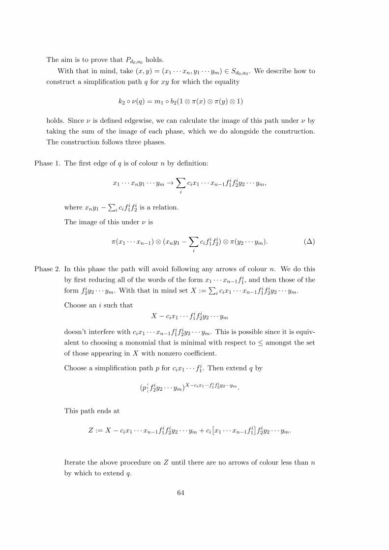
The aim is to prove that Pd0,a0 holds.
With that in mind, take (x, y) = (x1 · · ·xn, y1 · · · ym) ∈ Sd0,a0 . We describe how to
construct a simplification path q for xy for which the equality
k2 ◦ ν(q) = m1 ◦ b2(1⊗ π(x)⊗ π(y)⊗ 1)
holds. Since ν is defined edgewise, we can calculate the image of this path under ν by
taking the sum of the image of each phase, which we do alongside the construction.
The construction follows three phases.
Phase 1. The first edge of q is of colour n by definition:
x1 · · ·xny1 · · · ym →∑i
cix1 · · ·xn−1fi1f
i2y2 · · · ym,
where xny1 −∑
i cifi1f
i2 is a relation.
The image of this under ν is
π(x1 · · ·xn−1)⊗ (xny1 −∑i
cifi1f
i2)⊗ π(y2 · · · ym). (∆)
Phase 2. In this phase the path will avoid following any arrows of colour n. We do this
by first reducing all of the words of the form x1 · · ·xn−1fi1, and then those of the
form f i2y2 · · · ym. With that in mind set X :=∑
i cix1 · · ·xn−1fi1f
i2y2 · · · ym.
Choose an i such that
X − cix1 · · · f i1f i2y2 · · · ym
doesn’t interfere with cix1 · · ·xn−1fi1f
i2y2 · · · ym. This is possible since it is equiv-
alent to choosing a monomial that is minimal with respect to ≤ amongst the set
of those appearing in X with nonzero coefficient.
Choose a simplification path p for cix1 · · · f i1. Then extend q by
(p 999f i2y2 · · · ym)X−cix1···f
i1fi2y2···ym .
This path ends at
Z := X − cix1 · · ·xn−1fi1f
i2y2 · · · ym + ci
[x1 · · ·xn−1f
i1
]f i2y2 · · · ym.
Iterate the above procedure on Z until there are no arrows of colour less than n
by which to extend q.
64

Now we repeat this phase but for arrows of colour greater than n. In this way we
arrive at
Y :=∑
ci[x1 · · ·xn−1f
i1
][f i2y2 · · · ym
].
The image of the path in this phase is calculated by taking pi a simplification
path for x1 · · · f i1 and qi is a simplification path for f i2 · · · ym. Then we have:∑i
ci ν(pi)π(f i2y2 · · · ym
)+ ciπ
([x1 · · · f i1
])ν(qi). (Ξ)
We have used Lemma 4.5.6 in order to evaluate the image of the stitched and
translated paths.
Phase 3. Set Mij and Nij to be monomials in PBW order and dij ∈ K∗ such that:
Y =∑
ci([x1 · · ·xn−1f
i1
])([f i2y2 · · · ym
]) =
∑i
ci∑j
dijMijNij .
We choose a monomial m such that (Y • m) 6= 0 and Y − m doesn’t interfere
with m. We know that m is of the form czw for a constant c ∈ K∗ and a pair
(z, w) ∈ Sd with deg(z) = n. Since m ≤ xy, by Lemma 4.5.3 we know that
BG(m) appears as a proper subgraph of BG(xy) rooted at Y . In particular, since
the first arrow of q was of colour n, we know that BG(m) must have has strictly
fewer n-coloured arrows than BG(xy). Therefore, (z, w) ∈ Sd,a with a < a0 so
that we can apply the inductive hypothesis (b) and obtain a simplification path
for m, say pm, for which
k2 ◦ ν(pm) = m1 ◦ b2(c⊗ z ⊗ w ⊗ 1).
Then extend q by pY−mm . Iterate this over all of the terms in Y until q terminates
at[xy].
The image under ν of this phase is∑m
ν(pm), (Ψ)
which by the induction hypothesis satisfies∑m
k2 ◦ ν(pm) =∑i
ci(∑j
m1 ◦ b2(dij ⊗ π(Mij)⊗ π(Nij)⊗ 1)).
From here on we use labels in our equations to label the expression on the line that
the label appears, rather than the equation as a whole. Applying k2 to ν(q), we have
65
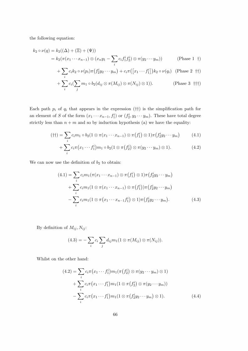
the following equation:
k2 ◦ ν(q) = k2((∆) + (Ξ) + (Ψ))
= k2(π(x1 · · ·xn−1)⊗ (xny1 −∑i
cifi1f
i2)⊗ π(y2 · · · ym)) (Phase 1 †)
+∑i
cik2 ◦ ν(pi)π(f i2y2 · · · ym
)+ ciπ
([x1 · · · f i1
])k2 ◦ ν(qi) (Phase 2 ††)
+∑i
ci(∑j
m1 ◦ b2(dij ⊗ π(Mij)⊗ π(Nij)⊗ 1)). (Phase 3 †††)
Each path pi of qi that appears in the expression (††) is the simplification path for
an element of S of the form (x1 · · ·xn−1, fi1) or (f i2, y2 · · · ym). These have total degree
strictly less than n+m and so by induction hypothesis (a) we have the equality:
(††) =∑i
cim1 ◦ b2(1⊗ π(x1 · · ·xn−1)⊗ π(f i1)⊗ 1)π
(f i2y2 · · · ym
)(4.1)
+∑i
ciπ(x1 · · · f i1
)m1 ◦ b2(1⊗ π
(f i2)⊗ π(y2 · · · ym)⊗ 1). (4.2)
We can now use the definition of b2 to obtain:
(4.1) =∑i
cim1(π(x1 · · ·xn−1)⊗ π(f i1)⊗ 1)π
(f i2y2 · · · ym
)+∑i
cim1(1⊗ π(x1 · · ·xn−1)⊗ π(f i1))π(f i2y2 · · · ym
)−∑i
cim1(1⊗ π(x1 · · ·xn−1f
i1
)⊗ 1)π
(f i2y2 · · · ym
). (4.3)
By definition of Mij , Nij :
(4.3) = −∑i
ci∑j
dijm1(1⊗ π(Mij)⊗ π(Nij)).
Whilst on the other hand:
(4.2) =∑i
ciπ(x1 · · · f i1
)m1(π
(f i2)⊗ π(y2 · · · ym)⊗ 1)
+∑i
ciπ(x1 · · · f i1
)m1(1⊗ π
(f i2)⊗ π(y2 · · · ym))
−∑i
ciπ(x1 · · · f i1
)m1(1⊗ π
(f i2y2 · · · ym
)⊗ 1). (4.4)
66

Now by definition:
(4.4) = −∑i
ci∑j
dijm1(π(Mij)⊗ π(Nij)⊗ 1).
We now consider (†††). By using the definition of b2 we obtain:
(†††) =∑i
ci∑j
m1(dij ⊗ π(Mij)⊗ π(Nij)) (4.5)
+∑i
ci∑j
m1(dijπ(Mij)⊗ π(Nij)⊗ 1) (4.6)
−∑i
ci∑j
m1(dij ⊗ π(MijNij)⊗ 1).
Note that:
(4.5) + (4.3) = 0 and (4.6) + (4.4) = 0.
After these calculations we can rewrite k2 ◦ ν(q) as:
k2 ◦ ν(q) = k2(π(x1 · · ·xn−1)⊗ (xny1 −∑i
cifi1f
i2)⊗ π(y2 · · · ym))
+∑i
cim1(π(x1 · · ·xn−1)⊗ π(f i1)⊗ 1)π
(f i2y2 · · · ym
)+∑i
cim1(1⊗ π(x1 · · ·xn−1)⊗ π(f i1))π(f i2y2 · · · ym
) (From (4.1))
+∑i
ciπ(x1 · · · f i1
)m1(π
(f i2)⊗ π(y2 · · · ym)⊗ 1)
+∑i
ciπ(x1 · · · f i1
)m1(1⊗ π
(f i2)⊗ π(y2 · · · ym))
(From (4.2))
−∑i
ci∑j
m1(dij ⊗ π(MijNij)⊗ 1).
Call the right hand side of the above expression (∗).
We now calculate:
m1 ◦ b2(1⊗ π(x)⊗ π(y)⊗ 1) = m1(π(x)⊗ π(y)⊗ 1) (4.7)
−m1(1⊗ π(xy)⊗ 1) (4.8)
+m1(1⊗ π(x)⊗ π(y)). (4.9)
67

Recall that by definition
π(xy) = π([xy])
= π
∑i
ci
∑j
dijMijNij
,so that:
(4.8) = −∑i
ci∑j
m1(dij ⊗ π(MijNij)⊗ 1).
Furthermore, by the definition of m1 we have:
(4.7) =∑i
(ciπ(x1 · · · f i1
)m1(π
(f i2)⊗ π(y2 · · · ym)⊗ 1)
)+ π(x1 · · ·xn)⊗ y1 ⊗ π(y2 · · · ym)
and
(4.9) =∑i
(cim1(1⊗ π(x1 · · ·xn−1)⊗ π
(f i1))π(f i2y2 · · · ym
))+ π(x1 · · ·xn−1)⊗ xn ⊗ π(y1 · · · ym).
We can therefore rewrite (∗) as:
k2 ◦ ν(q) = k2
(π(x1 · · ·xn−1)⊗ (xny1 −
∑i
cifi1f
i2)⊗ π(y2 · · · ym)
)+∑i
cim1
(π(x1 · · ·xn−1)⊗ π
(f i1)⊗ 1)π(f i2y2 · · · ym
)+ (4.7)− π(x1 · · ·xn−1)⊗ xn ⊗ π(y1 · · · ym)
+ (4.9)− π(x1 · · ·xn)⊗ y1 ⊗ π(y2 · · · ym).
+∑i
ciπ(x1 · · · f i1
)m1
(1⊗ π
(f i2)⊗ π(y2 · · · ym)
)+ (4.8).
68
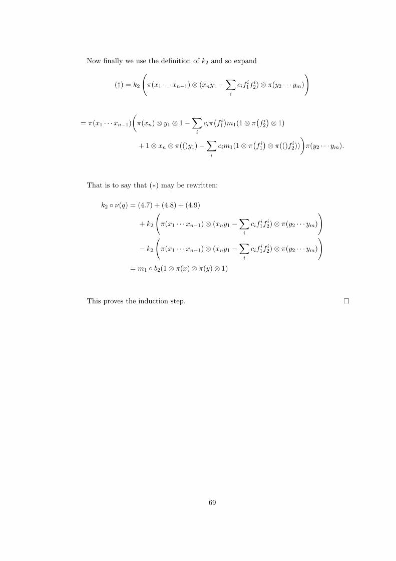
Now finally we use the definition of k2 and so expand
(†) = k2
(π(x1 · · ·xn−1)⊗ (xny1 −
∑i
cifi1f
i2)⊗ π(y2 · · · ym)
)
= π(x1 · · ·xn−1)
(π(xn)⊗ y1 ⊗ 1−
∑i
ciπ(f i1)m1(1⊗ π
(f i2)⊗ 1)
+ 1⊗ xn ⊗ π(()y1)−∑i
cim1(1⊗ π(f i1)⊗ π(()f i2))
)π(y2 · · · ym).
That is to say that (∗) may be rewritten:
k2 ◦ ν(q) = (4.7) + (4.8) + (4.9)
+ k2
(π(x1 · · ·xn−1)⊗ (xny1 −
∑i
cifi1f
i2)⊗ π(y2 · · · ym)
)
− k2
(π(x1 · · ·xn−1)⊗ (xny1 −
∑i
cifi1f
i2)⊗ π(y2 · · · ym)
)= m1 ◦ b2(1⊗ π(x)⊗ π(y)⊗ 1)
This proves the induction step.
69

70

Chapter 5
Primary Obstructions to
Infinitesimal Deformations
5.1 Introduction
In Chapter 3 we calculated the degree two component of the second Hochschild cohomol-
ogy of two algebras. As discussed in that chapter, this is equivalent to calculating the
set of isomorphism classes of infinitesimal deformations of these two algebras. However,
it is generally a much harder question to establish whether any of these infinitesimal
deformations integrate to formal deformations.
One possible first step in answering this question of integration is to calculate the
subset of infinitesimal deformations which have vanishing primary obstruction. By work
of Gerstenhaber (see Proposition 2.3.17), this is equivalent to calculating the subset of
HH22(C) of elements f such that [f, f ] is zero in cohomology. Recall from Definition
2.3.15 that for elements f, g ∈ B2 the Gerstenhaber bracket is defined on pure tensors
by
[f, g] (1|c1|c2|c3|1) = f(1|g(1|c1|c2|1)|c3|1)− f(1|c1|g(1|c2|c3|1)|1)+
g(1|f(1|c1|c2|1)|c3|1)− g(1|c1|f(1|c2|c3|1)|1)
In general, determing this set of infinitesimal deformations is difficult. Our method
relies upon the map m2 from Chapter 4 to reduce the problem to one that is amenable to
a computer script. We first give an overview of the theory behind the calculation, before
explaining the details of applying this theory to the two algebras discussed previously,
A and Aq. Note that the implementation details of m2 and the Gerstenhaber bracket
can be found in Appendix B.
71
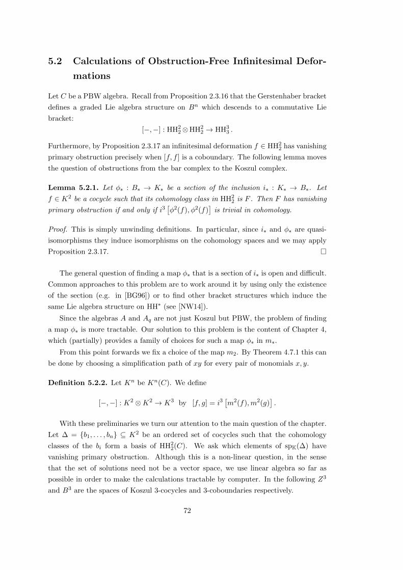
5.2 Calculations of Obstruction-Free Infinitesimal Defor-
mations
Let C be a PBW algebra. Recall from Proposition 2.3.16 that the Gerstenhaber bracket
defines a graded Lie algebra structure on Bn which descends to a commutative Lie
bracket:
[−,−] : HH22⊗HH2
2 → HH33 .
Furthermore, by Proposition 2.3.17 an infinitesimal deformation f ∈ HH22 has vanishing
primary obstruction precisely when [f, f ] is a coboundary. The following lemma moves
the question of obstructions from the bar complex to the Koszul complex.
Lemma 5.2.1. Let φ∗ : B∗ → K∗ be a section of the inclusion i∗ : K∗ → B∗. Let
f ∈ K2 be a cocycle such that its cohomology class in HH22 is F . Then F has vanishing
primary obstruction if and only if i3[φ2(f), φ2(f)
]is trivial in cohomology.
Proof. This is simply unwinding definitions. In particular, since i∗ and φ∗ are quasi-
isomorphisms they induce isomorphisms on the cohomology spaces and we may apply
Proposition 2.3.17.
The general question of finding a map φ∗ that is a section of i∗ is open and difficult.
Common approaches to this problem are to work around it by using only the existence
of the section (e.g. in [BG96]) or to find other bracket structures which induce the
same Lie algebra structure on HH∗ (see [NW14]).
Since the algebras A and Aq are not just Koszul but PBW, the problem of finding
a map φ∗ is more tractable. Our solution to this problem is the content of Chapter 4,
which (partially) provides a family of choices for such a map φ∗ in m∗.
From this point forwards we fix a choice of the map m2. By Theorem 4.7.1 this can
be done by choosing a simplification path of xy for every pair of monomials x, y.
Definition 5.2.2. Let Kn be Kn(C). We define
[−,−] : K2 ⊗K2 → K3 by [f, g] = i3[m2(f),m2(g)
].
With these preliminaries we turn our attention to the main question of the chapter.
Let ∆ = {b1, . . . , bn} ⊆ K2 be an ordered set of cocycles such that the cohomology
classes of the bi form a basis of HH22(C). We ask which elements of spK(∆) have
vanishing primary obstruction. Although this is a non-linear question, in the sense
that the set of solutions need not be a vector space, we use linear algebra so far as
possible in order to make the calculations tractable by computer. In the following Z3
and B3 are the spaces of Koszul 3-cocycles and 3-coboundaries respectively.
72

We start with a high level overview of the calculation. Our aim is to describe the
set
Λ := {f ∈ spK ∆ | f has vanishing primary obstruction } .
Let π : Z3 → HH3 be the canonical projection map. It is a fundamental fact of Ger-
stenhaber’s deformation theory (see Proposition 2.3.13) that [f, f ] ∈ Z3. Furthermore,
by Proposition 2.3.17 we can write Λ in terms of the Gerstenhaber bracket:
Λ = {f ∈ spK ∆ | π([f, f ]) = 0} .
We describe in detail how to find this set.
To start we factor the map f 7→ [f, f ] into linear and non-linear factors. Let K(n+12 )
have a chosen basis of
{vi,j | 1 ≤ i ≤ j ≤ n} .
Furthermore, let wi,j = [bi, bj ]. We define the linear map λ : K(n+12 ) → Z3 by
λ(vi,j) = wi,j .
On the other hand, we define the polynomial map
p : spK ∆→ K(n+12 )
∑i
aibi 7→∑i
a2i vi,i +
∑i<j
2aiajvi,j .
Lemma 5.2.3. For f ∈ spK ∆ we have
[f, f ] = λ ◦ p(f).
Proof. This follows from the commutativity and bilinearity properties of the Gersten-
haber bracket. In particular, if f =∑
i aibi then
[f, f ] =
∑i
aibi,∑j
ajbj
=∑i 6=j
aiaj [bi, bj ] +∑i
a2i [bi, bi]
=∑j>i
2aiaj [bi, bj ] +∑i
a2i [bi, bi]
= λ ◦ p(f).
73
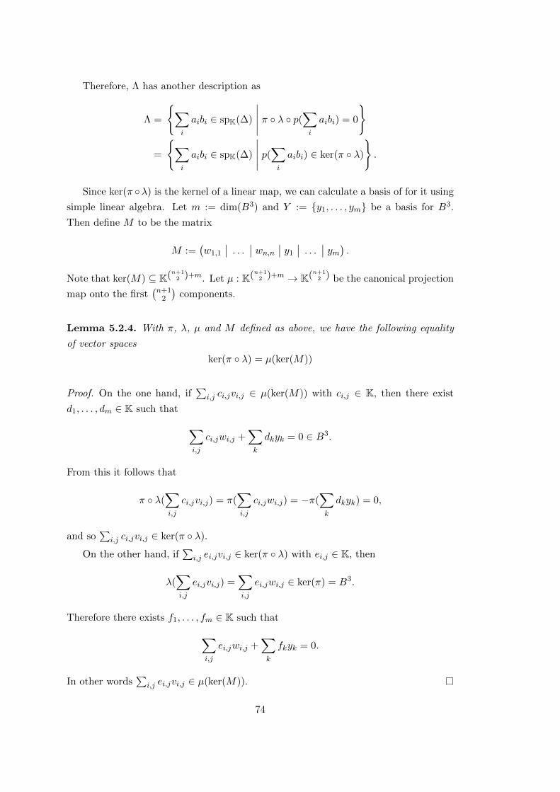
Therefore, Λ has another description as
Λ =
{∑i
aibi ∈ spK(∆)
∣∣∣∣∣ π ◦ λ ◦ p(∑i
aibi) = 0
}
=
{∑i
aibi ∈ spK(∆)
∣∣∣∣∣ p(∑i
aibi) ∈ ker(π ◦ λ)
}.
Since ker(π ◦λ) is the kernel of a linear map, we can calculate a basis of for it using
simple linear algebra. Let m := dim(B3) and Y := {y1, . . . , ym} be a basis for B3.
Then define M to be the matrix
M :=(w1,1
∣∣ . . . ∣∣ wn,n ∣∣ y1
∣∣ . . . ∣∣ ym) .Note that ker(M) ⊆ K(n+1
2 )+m. Let µ : K(n+12 )+m → K(n+1
2 ) be the canonical projection
map onto the first(n+1
2
)components.
Lemma 5.2.4. With π, λ, µ and M defined as above, we have the following equality
of vector spaces
ker(π ◦ λ) = µ(ker(M))
Proof. On the one hand, if∑
i,j ci,jvi,j ∈ µ(ker(M)) with ci,j ∈ K, then there exist
d1, . . . , dm ∈ K such that ∑i,j
ci,jwi,j +∑k
dkyk = 0 ∈ B3.
From this it follows that
π ◦ λ(∑i,j
ci,jvi,j) = π(∑i,j
ci,jwi,j) = −π(∑k
dkyk) = 0,
and so∑
i,j ci,jvi,j ∈ ker(π ◦ λ).
On the other hand, if∑
i,j ei,jvi,j ∈ ker(π ◦ λ) with ei,j ∈ K, then
λ(∑i,j
ei,jvi,j) =∑i,j
ei,jwi,j ∈ ker(π) = B3.
Therefore there exists f1, . . . , fm ∈ K such that∑i,j
ei,jwi,j +∑k
fkyk = 0.
In other words∑
i,j ei,jvi,j ∈ µ(ker(M)).
74

Therefore we may finally describe Λ as
Λ =
{∑i
aibi ∈ spK(∆)
∣∣∣∣∣ p(∑i
aibi) ∈ µ(ker(M))
}.
With this in mind, we calculate the space of f ∈ spK(∆) with vanishing primary
obstruction as follows.
1. For each pair{
(i, j) ∈ N2∣∣ 1 ≤ i ≤ j ≤ n
}calculate wi,j = [bi, bj ].
2. Choose a basis {y1, . . . , ym} of B3 and form the matrix
M =(w1,1
∣∣ . . . ∣∣ wn,n ∣∣ y1
∣∣ . . . ∣∣ ym) .3. Calculate the right kernel of M and choose a basis of µ(ker(M)) ⊆ K(n+1
2 ) ex-
pressed in terms of the basis {vi,j} of K(n+12 ).
4. Use the preceding step to deduce which f in spK(∆) have p(f) in µ(Ker(M)).
In the above calculation, steps 1-3 are entirely computer based. Most of the com-
puting time is concentrated in step 1 as this involves the long calculation of paths in
Bergman graphs in order to find the Gerstenhaber bracket using m2. The rest of the
computation consists mostly of Gaussian elimination which ‘Sage’ implements to be
relatively fast. The output of the computer calculations is a basis of µ(ker(M)). After
this basis is determined we reason by hand to compute the set Λ.
For example, we will see that in both of the cases of interest C = A or Aq that
v1,1 appears in the output basis of µ(ker(M)). From the definition of p it follows that
p(a1b1) ∈ µ(ker(M)), and therefore a1b1 ∈ Λ and has vanishing primary obstruction.
Note that in general determining elements of Λ is more complicated than this example.
In Section 5.3 we go through an example by hand in the context of the algebra A
to make the above more concrete before explaining the computer code and discussing
the output.
5.3 The Obstruction-Free Infinitesimal Deformations of A
We apply the calculations in Section 5.2 in the context of the algebra A. Recall that
from Section 3.3 we know that we can choose ∆ = {b1, . . . , b8} to be the ordered set:
75

x1x3
0
0
x2x3
x1x4
0
x23
0
x1x4
0
0
x3x4
x21
0
0
x2x1
x2x3
0
0
x2x4
0
0
x1x4
0
0
x24
0
0
x3x4
0
0
x22
0
0
x2x3
0
0
0
0
x21
0
−x1x3
0
0
0
−x22
0
x2x4
Example 5.3.1. To understand the following calculations an example worked through
by hand may be helpful. Recall that A has six relations
R =
{r1 := x3x1 − x1x3, r2 := x4x2 − x2x4, r3 := x4x1 − x2x3
r4 := x1x2 − x2x3, r5 := x3x2 − x1x4, r6 := x4x3 − x1x4
},
and four doubly defined relations
D :=
{d1 := x3r4 + x1(r6 − r5) = r1x2 − r5x3, d2 := x4r1 − x1r3 = r6x1 + (r4 − r3)x3
d3 := x4r5 − x1r2 = r6x2 + (r4 − r3)x4 d4 := x4r4 + x2(r6 − r5) = r3x2 − r2x3
}.
We calculate [f, f ] for
f :=
x23
0
x1x4
0
0
x3x4
= b2 ∈ ∆.
Recall that under the vector notation, f is a function that maps r2, r4 and r5 to
zero and r1, r3 and r6 to x23, x1x4 and x3x4 respectively. Now, [f, f ] is a function
defined on K3 and so we write it as
[f, f ] = i3[m2(f),m2(f)
]=
Θ1
Θ2
Θ3
Θ4
using the vector notation introduce in Notation 3.2.1, so that [f, f ] sends di to Θi. We
76

now calculate Θ1. We remind the reader that we use the | symbol to represent ⊗K.
Θ1 =[m2(f),m2(f)
](d1) = 2(m2(f) ◦m2(f))(d1)
= 2m2(f)(1|m2(f)(1|r1|1)|x2|1− 1|m2(f)(1|r5|1)|x3|1)
− 2m2(f)(1|x3|m2(f)(1|r4|1)|1 + 1|x1|m2(f)(1|r6|1)|1− 1|x1|m2(f)(1|r5|1)|1).
Recall that m2 is a section of the inclusion map from K2 = A⊗R⊗A into B2, and so
acts trivially on relations. That is to say that for any relation ri we have
m2(f)(1|ri|1) = f(m2(1|ri|1)) = f(1|ri|1).
Therefore, the above continues as:
Θ1 = 2(m2(f)(1|x2
3|x2|1− 0)−m2(f)(0 + 1|x1|x3x4|1− 0))
= 2f(m2(1|x2
3|x2|1)−m2(1|x1|x3x4|1)).
The map m2 is defined on a pure tensor 1|x|y|1 by choosing a simplification path
of xy in the graph BG(xy) and evaluating the function ν on this path (see Section 4.7
for details). In particular, since x1x3x4 is in PBW order we can apply the reasoning of
Lemma 4.7.3 and deduce that
m2(1|x1|x3x4|1) = 0.
As for x23x2, the Bergman graph is as follows:
x23x2 x3x1x4 x1x3x4.
rx3r5 rr1x4
Since there is a unique simplification path in this Bergman graph,
m2(1|x23|x2|1) = x3|r5|1 + 1|r1|x4,
and so
Θ1 = 2f(x3|r5|1 + 1|r1|x4) = 2x23x4.
The rest of the calculations of the Θi’s follows similarly and we obtain that
[f, f ] = 2
x2
3x4
−x1x3x4
0
0
.
77
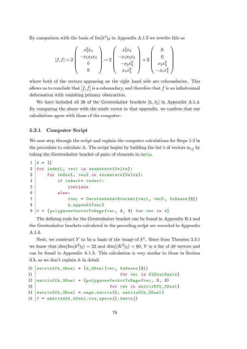
By comparison with the basis of Im(k3)2 in Appendix A.1.3 we rewrite this as
[f, f ] = 2
x2
3x4
−x1x3x4
0
0
= 2
x2
3x4
−x1x3x4
−x3x24
x1x24
+ 2
0
0
x3x24
−x1x24
where both of the vectors appearing on the right hand side are coboundaries. This
allows us to conclude that [f, f ] is a coboundary, and therefore that f is an infinitesimal
deformation with vanishing primary obstruction.
We have included all 36 of the Gerstenhaber brackets [bi, bj ] in Appendix A.1.4.
By comparing the above with the ninth vector in that appendix, we confirm that our
calculations agree with those of the computer.
5.3.1 Computer Script
We now step through the script and explain the computer calculations for Steps 1-3 in
the procedure to calculate Λ. The script begins by building the list W of vectors wi,j by
taking the Gerstenhaber bracket of pairs of elements in Delta.
1 W = []
2 for index1 , vec1 in enumerate(Delta):
3 for index2 , vec2 in enumerate(Delta):
4 if index2 < index1:
5 continue
6 else:
7 func = GerstenhaberBracket(vec1 , vec2 , KnBases [3])
8 W.append(func)
9 W = [polygnomeVectorToSage(vec , 3, 3) for vec in W]
The defining code for the Gerstenhaber bracket can be found in Appendix B.4 and
the Gerstenhaber brackets calculated in the preceding script are recorded in Appendix
A.1.4.
Next, we construct Y to be a basis of the image of k3. Since from Theorem 3.3.1
we know that dim(Im(k2)2) = 22 and dim((K2)2) = 60, Y is a list of 38 vectors and
can be found in Appendix A.1.3. This calculation is very similar to those in Section
3.3, so we don’t explain it in detail.
10 matrixOfk_3Dual = [k_3Dual(vec , KnBases [3])
11 for vec in K2DualBasis]
12 matrixOfk_3Dual = [polygnomeVectorToSage(vec , 3, 3)
13 for vec in matrixOfk_3Dual]
14 matrixOfk_3Dual = sage.matrix(K, matrixOfk_3Dual)
15 Y = matrixOfk_3Dual.row_space (). basis ()
78
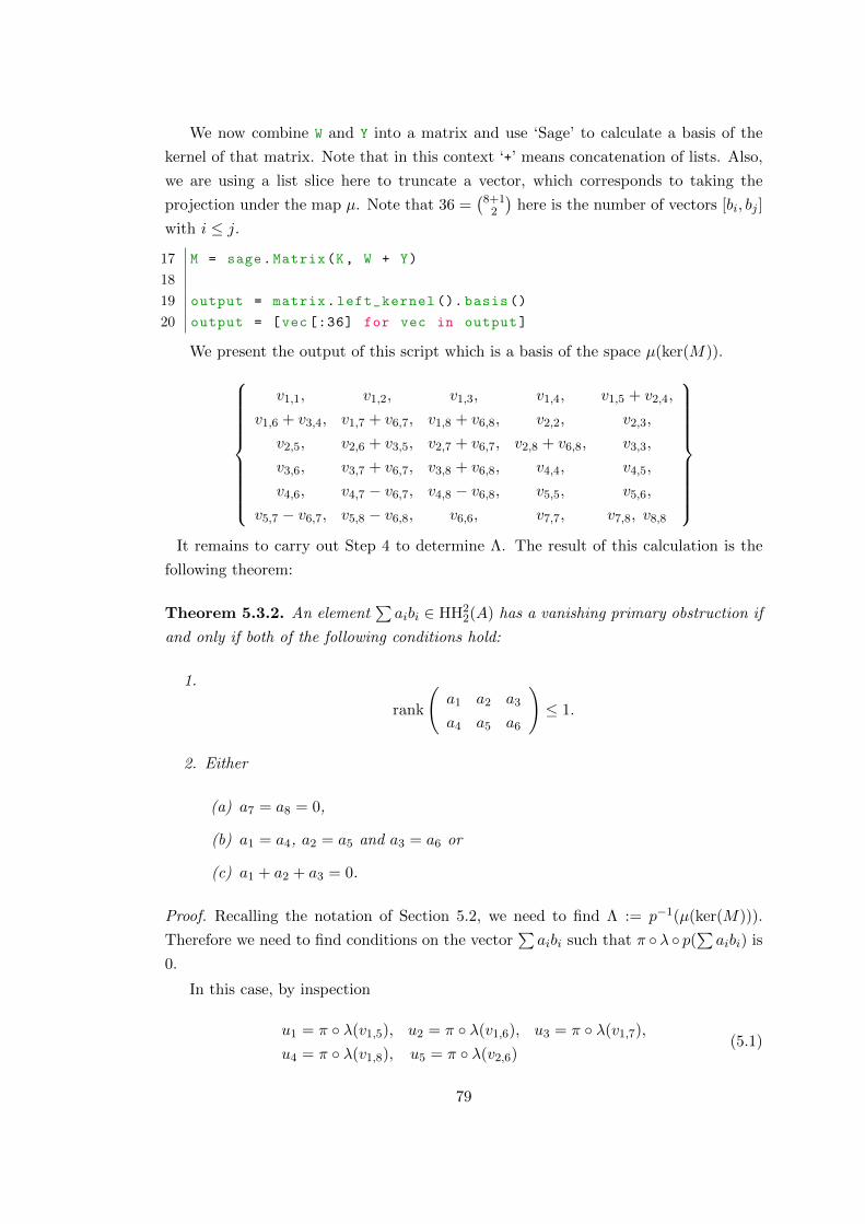
We now combine W and Y into a matrix and use ‘Sage’ to calculate a basis of the
kernel of that matrix. Note that in this context ‘+’ means concatenation of lists. Also,
we are using a list slice here to truncate a vector, which corresponds to taking the
projection under the map µ. Note that 36 =(
8+12
)here is the number of vectors [bi, bj ]
with i ≤ j.
17 M = sage.Matrix(K, W + Y)
18
19 output = matrix.left_kernel (). basis()
20 output = [vec [:36] for vec in output]
We present the output of this script which is a basis of the space µ(ker(M)).
v1,1, v1,2, v1,3, v1,4, v1,5 + v2,4,
v1,6 + v3,4, v1,7 + v6,7, v1,8 + v6,8, v2,2, v2,3,
v2,5, v2,6 + v3,5, v2,7 + v6,7, v2,8 + v6,8, v3,3,
v3,6, v3,7 + v6,7, v3,8 + v6,8, v4,4, v4,5,
v4,6, v4,7 − v6,7, v4,8 − v6,8, v5,5, v5,6,
v5,7 − v6,7, v5,8 − v6,8, v6,6, v7,7, v7,8, v8,8
It remains to carry out Step 4 to determine Λ. The result of this calculation is the
following theorem:
Theorem 5.3.2. An element∑aibi ∈ HH2
2(A) has a vanishing primary obstruction if
and only if both of the following conditions hold:
1.
rank
(a1 a2 a3
a4 a5 a6
)≤ 1.
2. Either
(a) a7 = a8 = 0,
(b) a1 = a4, a2 = a5 and a3 = a6 or
(c) a1 + a2 + a3 = 0.
Proof. Recalling the notation of Section 5.2, we need to find Λ := p−1(µ(ker(M))).
Therefore we need to find conditions on the vector∑aibi such that π ◦λ ◦ p(
∑aibi) is
0.
In this case, by inspection
u1 = π ◦ λ(v1,5), u2 = π ◦ λ(v1,6), u3 = π ◦ λ(v1,7),
u4 = π ◦ λ(v1,8), u5 = π ◦ λ(v2,6)(5.1)
79

form a basis of Im(π ◦ λ). With that basis in mind, π sends any vi,j to zero except
those in (5.1) and:
π ◦ λ(v2,4) = −u1, π ◦ λ(v3,4) = −u2, π ◦ λ(v3,5) = −u5,
π ◦ λ(v2,7) = u3, π ◦ λ(v3,7) = u3, π ◦ λ(v4,7) = −u3,
π ◦ λ(v5,7) = −u3, π ◦ λ(v6,7) = −u3, π ◦ λ(v2,8) = u4,
π ◦ λ(v3,8) = u4, π ◦ λ(v4,8) = −u4, π ◦ λ(v5,8) = −u4, π ◦ λ(v6,8) = −u4.
Therefore we have that, with respect to the basis {ui}
π ◦ λ ◦ p(∑
aibi) =
2(a1a5 − a2a4)
2(a1a6 − a3a4)
2(a1 + a2 + a3 − a4 − a5 − a6)a7
2(a1 + a2 + a3 − a4 − a5 − a6)a8
2(a2a6 − a3a5)
.
This is zero precisely when the conditions in the statement of the proposition hold.
Therefore the set of infinitesimal deformations with vanishing primary obstructions
is a variety lying in HH22∼= K8. The variety decomposes into the union of three
components, namely:
Vg :={
(a1, . . . , a8) ∈ K8∣∣ a1 = a4, a2 = a5 and a3 = a6
},
Vq :=
{(a1, . . . , a8) ∈ K8
∣∣∣∣∣ a7 = a8 = 0 and rank
(a1 a2 a3
a4 a5 a6
)≤ 1
}and
Vu =
{(a1, . . . , a8) ∈ K8
∣∣∣∣∣ a1 + a2 + a3 = 0 and rank
(a1 a2 a3
a4 a5 a6
)≤ 1
}.
From these definitions it is clear that Vg is a five dimensional vector subspace of
K8, Vu is a five dimensional variety and Vq is a four dimensional determinental variety.
We also list the intersections of these three varieties, all of which lie in K8.
• Vg ∩ Vq is a three dimensional vector space
{(a1, a2, a3, a1, a2, a3, 0, 0) ∈ K8
}.
80

• Vg ∩ Vu is a four dimensional vector space
{(a1, a2, a3, a1, a2, a3, a7, a8) | a1 + a2 + a3 = 0} .
• Vq ∩ Vu is a three dimensional (non-linear) variety
{(a1, a2, a3, a4, a5, a6, 0, 0) | a1 + a2 + a3 = a4 + a5 + a6 = a3a5 − a2a6 = 0} .
• Vq ∩ Vg ∩ Vu is a two dimensional vector space
{(a1, a2, a3, a1, a2, a3, 0, 0) | a1 + a2 + a3 = 0} .
We will see later that these varieties correspond to some very different deformations.
For example, Vg will be shown to be the space of infinitesimals arising from deformations
of A defined in terms of automorphisms of surfaces birational to P1 × P1, and that all
deformations in Vg integrate. Such examples of deformations were the topic of the
paper [RS12]. All of these deformations are birationally commutative.
In contrast to this, Vq will be shown to contain the infinitesimal associated to
the family of deformations Aq. None of these are birationally commutative, having
a noncommutative rational function field of Kq(u, v). We are able to integrate most
deformations in Vq. In contrast, we know little about those lying in Vu.
5.4 The Obstruction-Free Infinitesimal Deformations of
Aq
We now turn our attention to Aq. We repeat the procedure outlined in Section 5.3 for
Aq. By work in Section 3.4 we know that we can choose ∆ to be the following set.
x1x3
0
0
x2x3
qx1x4
0
,
0
x2x4
0
0
x1x4
0
,
0
x24
0
0
x3x4
0
,
0
x22
0
0
x2x3
0
The ‘Sage’ script is almost identical to that in the preceding section so we will not
go through it line by line. Note that since ∆ is of size 4, we have truncated the vectors
to the first 10 =(
4+12
)entries.
81

1 W = []
2 for index1 , vec1 in enumerate(Delta):
3 for index2 , vec2 in enumerate(Delta):
4 if index2 < index1:
5 continue
6 else:
7 func = GerstenhaberBracket(vec1 , vec2 ,
8 qKnBases [3])
9 W.append(func)
10 W = [polygnomeVectorToSage(vec , 3, 3) for vec in W]
11
12
13 matrixOfk_3Dual = [k_3Dual(vec , qKnBases [3])
14 for vec in qK2DualBasis]
15 matrixOfk_3Dual = [polygnomeVectorToSage(vec , 3, 3)
16 for vec in matrixOfk_3Dual]
17 matrixOfk_3Dual = sage.matrix(K, matrixOfk_3Dual)
18 Y = matrixOfk_3Dual.row_space (). basis ()
19
20 M = sage.Matrix(K, W + Y)
21
22 output = matrix.left_kernel (). basis()
23 output = [vec [:10] for vec in output]
The output of this script is the basis of µ(ker(M).{v1,1 v1,2 v1,3 v1,4 v2,2
v2,3 v2,4 v3,3 v3,4 v4,4
}
Notice that this is the standard basis of K10.
Proposition 5.4.1. All infinitesimal deformations of Aq have vanishing primary ob-
struction.
Proof. Since µ(ker(M)) = K10, the condition p(f) ∈ µ(ker(M)) is trivial. Therefore
the set Λ of infinitesimal deformations with vanishing primary obstruction is
p−1(K10) = HH22(Aq).
If HH33(Aq) were trivial then we could immediately deduce that all infinitesimal de-
formations integrate to formal deformations. However, we note briefly that HH33(Aq) 6=
0 by calculations similar to those in Section 3.3 so that this result is not a priori obvious.
We shall return to this question in Chapter 7.
82
Chapter 6
Infinitesimal Deformations
Arising From Automorphisms of
Minimal Rational Surfaces
6.1 Introduction
In this chapter we discuss some of the infinitesimal deformations of the algebra A.
Recall that if
E = {t, ut, vt, uvt} ⊆ K(u, v)[t;σ]
then A ∼= K〈E〉. In [RS12] it is shown that for a certain family {τ} ⊆ Aut(K(u, v)) the
set
E′ = {t, ut, vt, uvt} ⊆ K(u, v)[t;σ ◦ τ ]
generates a family of deformations of A. The aim of this chapter is to investigate the
infinitesimal structure of such deformations but generalised in two directions: firstly
to the whole Lie algebra of the automorphism group of P1 × P1 and secondly to Lie
algebras of automorphism groups of other surfaces entirely.
In particular, we answer two questions.
1. What infinitesimal deformations arise due to the deformations of Qgr(A) discussed
in [RS12]?
2. Does expanding the set of automorphisms considered to those of other minimal
rational surfaces increase the space of infinitesimal deformations that occur?
We show in Theorem 6.4.1 that the answer to the first question is precisely the set
Vg. In Theorems 6.5.1 and 6.6.2 we show that the answer to the second question is no.
This is a strong signal that in order to find new families of deformations of A, we need
to concentrate on rings that are not birationally commutative.
83

Notation 6.1.1. In this chapter we change notation slightly to agree better with that
in [RS12]. From this point onwards, in this chapter only, we write σ for the birational
self map of P1 × P1 given by
[x : y][z : w] 799K [xz : yw][z : w]
On the other hand, the automorphism of K(u, v) previously referred to by σ will now be
written σ∗. That is to say that σ∗ is the automorphism of K(u, v) induced by choosing
coordinates on P1 × P1 of
u =x
yand v =
z
w,
so that
σ∗(u) = uv and σ∗(v) = v.
We hope this does not cause confusion.
Consider D := K(u, v)[t, t−1;σ∗], the graded quotient ring of A. If G is a Lie group
acting faithfully on K(u, v) and τ∗s is a one-parameter subgroup inside G, i.e. τ∗s is the
exponential of a one-dimensional subspace of Lie(G), then D(s) := K(u, v)[t, t−1;σ∗◦τ∗s ]
is a one-parameter family of deformations of D. In particular, in a formal neighbour-
hood of s = 0, we obtain an associative multiplication F on the vector space D⊗KK[[s]]
given by the K[[s]]-linear extension of
F (c, d) = cd+
∞∑i=1
Fi(c, d)si
for any c, d in D. In this case F1 defines an infinitesimal deformation of D (see Section
2.3). In this chapter our aim is to examine the relationship of such deformations with
infinitesimal deformations of A.
In particular, we define a linear map Φ : Lie(G)→ HH22(D). Furthermore, we shall
construct a linear map Λ : HH22(A) → HH2
2(D). In Section 6.2 we prove that there is
a tractable method for testing if a given L ∈ Lie(G) satisfies Φ(L) ∈ Im Λ: evaluating
Φ(L) on R ⊆ D ⊗D, where R is the set of relations of A, and testing if this lies in A.
That is to say we develop a method for taking certain elements of Lie(G) and producing
from them infinitesimal deformations of A.
Definition 6.1.2. If a vector L in Lie(G) satisfies Φ(L) ∈ Im(Λ) then we refer to it as
an admissible direction.
We then apply this test in the following natural situation. If Y is a minimal surface
birational to P1 × P1, then Y is P2 or Fn for n 6= 1 [Bea96, Theorem V.10]. In each
case, Aut(Y ) is a Lie group which we can regard as subgroup of the plane Cremona
group [DI09, Section 4], and we can consider the associated Lie algebra. Following a
84
calculation detailed below, we determine which infinitesimal deformations of A arise
from these Lie algebras.
6.2 Infinitesimal Deformations of a Localisation
In this section we construct a map Λ : HH22(A) → HH2
2(D) and show that there is a
simple test for whether a given f ∈ HH22(D) lies in Im(Λ): check that f(R) ⊆ A. This
is the foundation for the rest of this chapter, in which we apply this test in several
related situations. The results of this section do not depend on the PBW property of
A, nor on the fact that D is the graded quotient ring of A. For that reason we work
with more general algebras C and E.
Let C be a Koszul K-algebra that is a domain. Recall the definition of Ore sets and
localisation from Section 2.2.1. Recall further that the category of right modules over
the enveloping algebra Ce = C ⊗ Cop is equivalent to the category of C-bimodules.
Notation 6.2.1. For elements in r, s ∈ Cop we will always write r ∗op s to be the
opposite multiplication and rs to be the element of the underlying vector space C, i.e.
under the usual multiplication. As previously stated, we write tensor products over Kas unadorned tensor products ⊗.
Let E be a localisation of C with respect to some (left and right) Ore set S. We want
to compare the infinitesimal deformations of C with those of E. This is equivalent to
making a comparison between second Hochschild cohomology groups, i.e. second Ext
groups. In fact we find that in the case of Koszul algebras, there is a finite dimensional
test on infinitesimal deformations of E to determine if they correspond to deformations
of C.
First we need some basic module theoretic facts regarding the enveloping algebra.
In the following we set T to be the set S ⊗ S.
Proposition 6.2.2. (i) If C is a K-algebra and X a right (resp. left) Ore set with
respect to some spanning set B of C with X ⊆ B, then X is a right (resp. left)
Ore set for R.
(ii) T is a right and left Ore set for Ce.
(iii) Ee is the localisation of Ce with respect to T on the right (or left). In particular,
Ee is flat as a right or left Ce-module.
Before we prove Proposition 6.2.2 we state a useful lemma on localisation.
Lemma 6.2.3 ([MR01, Lemma 2.1.6]). Ee ∼= (Ce)T if and only if Ee satisfies the
following universal property: if Z is a ring and φ : Ce → Z is a ring homomorphism
such that all elements of φ(T ) are invertible in Z, then φ factors through Ee.
85
Proof of Proposition 6.2.2. We prove each statement in the right hand case, the left
hand case follows mutatis mutandis and it is clear due to the symmetry in the definitions
that there are no special considerations depending on handedness.
(i) In order to prove the Ore condition, take x ∈ X and a finite sum r :=∑
i cibi ∈ Cfor some bi ∈ B and ci ∈ K. By hypothesis we know that for all i there exists an
xi ∈ X and ai ∈ B such that bixi = xai.
Also, the set x1B ∩ . . . xnB ∩X is nonempty for any x1, . . . , xn ∈ X. This fact is
a very slight modification of the first part of [GW04, Lemma 4.21 (a)] where, in
this case, we do not know that X is an Ore set for the whole ring. However the
proof requires no changes. Therefore we may take t ∈ x1B ∩ . . . ∩ xnB ∩X, and
choose ri ∈ B for each i such that xiri = t ∈ X.
Then the following holds:(∑i
cibi
)t =
∑i
cibixiri =∑i
cixairi = x
(∑i
ciairi
)∈ rX ∩ xR.
Since B is a spanning set we know that any r ∈ C can be written as such a finite
sum and so this completes the proof.
(ii) To prove the right Ore condition we take pure tensors a⊗ b ∈ Ce and s⊗ t ∈ T .
Then there exist m,n ∈ C and q, r ∈ S such that aq = sm and rb = nt by the
two Ore conditions on S. Then the following holds:
(a⊗ b)(q ⊗ r) = aq ⊗ (b ∗op r) = aq ⊗ rb = sm⊗ nt = (s⊗ t)(m⊗ n).
This proves that T is a right Ore set with respect to the pure tensors. But T is
itself a set of pure tensors, and the pure tensors span Ce, so we can apply part
(i) and conclude that T is a right Ore set for Ce.
(iii) The second part of this statement is a well known consequence of the first part
(see e.g. [MR01, Proposition 2.1.16 (ii)]), so it suffices to show the first part.
Since S is both a left and a right Ore set we can localise with respect to it on
either side and get the same ring [MR01, Corollary 2.1.6 (ii)]. So the following
holds:
Eop = (CS)op ∼= (SC)op.
This allows us to write elements of Eop as s−1a which makes the following con-
siderably neater.
Let Z be a ring and φ : Ce → Z be a map as in Lemma 6.2.3. Then we may
86
define ψ : Ee → Z by extending the following K-linearly:
ψ(as−1 ⊗ t−1b) = φ(a⊗ b)φ(s⊗ t)−1.
We must show that ψ is a ring homomorphism. It suffices to check that ψ is
multiplicative on pure tensors. To that aim, take two pure tensors in Ee, as−1 ⊗t−1b and cq−1⊗ r−1d. We know there exists some x⊗ y ∈ T and e⊗ f ∈ Ce such
that:
(c⊗ d)(x⊗ y) = (s⊗ t)(e⊗ f) (6.1)
by the Ore condition (ii). Furthermore by the definition of ψ the following holds:
ψ(as−1 ⊗ t−1b)ψ(cq−1 ⊗ r−1d) = φ(a⊗ b)φ(s⊗ t)−1φ(c⊗ d)φ(q ⊗ r)−1. (6.2)
Whereas, in Ee we have:
(as−1 ⊗ t−1b)(cq−1 ⊗ r−1d) = (a⊗ b)(s−1 ⊗ t−1)(c⊗ d)(q−1 ⊗ r−1)
= (a⊗ b)(e⊗ f)(x−1 ⊗ y−1)(q−1 ⊗ r−1)
= ae(qx)−1 ⊗ (yr)−1fb. (6.3)
Acting on this by ψ and then using the fact that φ is a ring homomorphism gives
us:
ψ(ae(qx)−1 ⊗ (yr)−1fb) = φ(ae⊗ fb)φ(qx⊗ yr)−1
= φ(a⊗ b)φ(e⊗ f)φ(x⊗ y)−1φ(q ⊗ r)−1. (6.4)
Finally using equation (6.1) we get that:
φ(c⊗ d)φ(x⊗ y) = φ(s⊗ t)φ(e⊗ f)
=⇒ φ(e⊗ f)φ(x⊗ y)−1 = φ(s⊗ t)−1φ(c⊗ d). (6.5)
So that:
ψ(as−1 ⊗ t−1b)ψ(cq−1 ⊗ r−1d) = φ(a⊗ b)φ(s⊗ t)−1φ(c⊗ d)φ(q ⊗ r)−1 by (6.2)
= φ(a⊗ b)φ(e⊗ f)φ(x⊗ y)−1φ(q ⊗ r)−1 by (6.5)
= ψ(ae(qx)−1 ⊗ (yr)−1fb) by (6.4)
= ψ((as−1 ⊗ t−1b)(cq−1 ⊗ r−1d)
)by (6.3).
87
This is the statement that ψ is multiplicative on pure tensors and is therefore a
ring homomorphism as required.
If we set ψ′ : Ce → Ee to be the obvious inclusion homomorphism it is immediate
that φ = ψ ◦ ψ′. By Lemma 6.2.3,
Ee ∼= (Ce)T .
Lemma 6.2.4. As right Ee modules, C ⊗Ce Ee is isomorphic to E.
Proof. We adopt the convention for writing pure tensor elements of C⊗CeEe as a|b⊗d,
so that the bar represents the tensor over Ce.
We define a map λ : C ⊗Ce Ee → E of Ee-modules by extending the following
Ee-linearly:
a|c−1 ⊗ e−1 7→ e−1ac−1.
Of course, since the | is a tensor over Ce, any pure tensor is of this form since:
a|bs−1 ⊗ t−1c = cab|s−1 ⊗ t−1.
In order to show that λ is an isomorphism, we define its inverse. Take d = ab−1 ∈ Eand set: δ(d) = a|b−1 ⊗ 1 ∈ C ⊗Ce Ee. If ab−1 = st−1 there are some x, y ∈ C such
that ay = sx and by = tx by the definition of localisation, so that
s|t−1 ⊗ 1 = s|xx−1t−1 ⊗ 1 = sx|x−1t−1 ⊗ 1
= ay|y−1b−1 ⊗ 1 = a|b−1 ⊗ 1
so δ is well defined.
We check that indeed δ = λ−1. Firstly, consider a|b−1 ⊗ t−1 ∈ C ⊗Ce Ee and note
that by the Ore condition we have elements m ∈ C, n ∈ S such that:
tm = an =⇒ mn−1 = t−1a,
where the second equality is in E. Then the following shows δλ is equal to idC⊗CeEe :
a|b−1 ⊗ t−1 λ7−→ t−1ab−1 = mn−1b−1
δ7−→ m|n−1b−1 ⊗ 1 = m|n−1b−1 ⊗ t−1t
= tm|n−1b−1 ⊗ t−1 = an|n−1b−1 ⊗ t−1
= a|b−1 ⊗ t−1.
88

It is also the case that λδ is equal to idE since the following holds, for d = ab−1 ∈ E:
λδ(d) = λδ(ab−1) = λ(a|b−1 ⊗ 1) = ab−1 = d.
Therefore λ = δ−1, and λ is an isomorphism.
Lemma 6.2.5. For X a vector space, the free right Ce-module C ⊗X ⊗ C satisfies:
(C ⊗X ⊗ C)⊗Ce Ee is naturally isomorphic to E ⊗X ⊗ E as right Ee-modules.
Here the right hand side module has multiplication
1⊗ z ⊗ 1(e⊗ e′) = e′ ⊗ z ⊗ e.
Proof. For a K-algebra ∆ and a vector space Γ, the equivalence of categories of C-
bimodules and right Ce-modules is given by the following isomorphism of right ∆e-
modules:
Γ⊗∆e ∼= ∆⊗ Γ⊗∆,
where the right hand side has module multiplication for γ ∈ Γ and δ, δ′ ∈ ∆:
(1⊗ γ ⊗ 1)(δ ⊗ δ′) = δ′ ⊗ γ ⊗ δ.
By definition, the free right Ce-module on X is X⊗Ce. This lemma is simply then
a reformulation of the fact that X ⊗Ce⊗Ce Ee is naturally isomorphic to X ⊗Ee.
Notation 6.2.6. Recall that C is a Koszul K-algebra which is a domain and E =
SC = CS is the localisation of C at a left and right Ore set S. Let K∗ = C⊗K∗⊗C be
the Koszul complex of C, B∗ be the bar resolution of C and i∗ : K∗ → B∗ the natural
inclusion (see Section 2.1 for definitions). Further, let
φ∗ : B∗ → K∗
be any section of i∗. Then let
I∗ : E ⊗K∗ ⊗ E → E ⊗ C⊗∗ ⊗ E
be the value of the functor −⊗Ce Ee at i∗, taking into account the isomorphism from
Lemma 6.2.5. Likewise, let
Φ∗ : E ⊗ C⊗∗ ⊗ E → E ⊗K∗ ⊗ E
be the value of −⊗Ce Ee at φ∗.
89
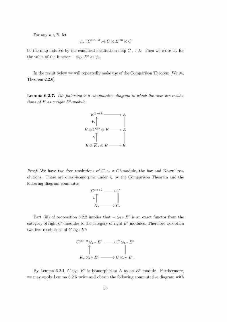
For any n ∈ N, let
ψn : C⊗n+2 ↪→ C ⊗ E⊗n ⊗ C
be the map induced by the canonical localisation map C ↪→ E. Then we write Ψ∗ for
the value of the functor −⊗Ce Ee at ψ∗.
In the result below we will repeatedly make use of the Comparison Theorem [Wei94,
Theorem 2.2.6].
Lemma 6.2.7. The following is a commutative diagram in which the rows are resolu-
tions of E as a right Ee-module:
E⊗∗+2 E
E ⊗ C⊗∗ ⊗ E E
E ⊗K∗ ⊗ E E.
Ψ∗
I∗
Proof. We have two free resolutions of C as a Ce-module, the bar and Koszul res-
olutions. These are quasi-isomorphic under i∗ by the Comparison Theorem and the
following diagram commutes
C⊗∗+2 C
K∗ C.
i∗
Part (iii) of proposition 6.2.2 implies that − ⊗Ce Ee is an exact functor from the
category of right Ce-modules to the category of right Ee modules. Therefore we obtain
two free resolutions of C ⊗Ce Ee:
C⊗∗+2 ⊗Ce Ee C ⊗Ce Ee
K∗ ⊗Ce Ee C ⊗Ce Ee.
By Lemma 6.2.4, C ⊗Ce Ee is isomorphic to E as an Ee module. Furthermore,
we may apply Lemma 6.2.5 twice and obtain the following commutative diagram with
90

exact rows:
E ⊗ C⊗∗ ⊗ E E
E ⊗K∗ ⊗ E E.
I∗
Finally, by the Comparison Theorem the bar resolution of E itself is quasi-isomorphic
to both of these resolutions. The chain map realising this is precisely Ψ∗, and so we
obtain the diagram in the lemma.
Notation 6.2.8. Let Λn : HomCe(C⊗n+2, C)→ HomEe(E ⊗C⊗n ⊗E,E) be the map
taking f ∈ HomCe(C⊗n+2, C) to the map defined on pure tensors by
Λn(f)(e⊗ c1 ⊗ . . .⊗ cn ⊗ e′) = ef(1⊗ c1 ⊗ . . .⊗ cn ⊗ 1)e′.
We note that each Λn is an injection whose image is
{g ∈ Hom(E ⊗ C⊗n ⊗ E,E)
∣∣ g(1⊗ C⊗n ⊗ 1) ⊆ C},
Furthermore, by the definition of the boundary map δ∗ on E ⊗ C⊗n ⊗ E and the
boundary map b∗ on C⊗n+2, it follows that δ∗(Λ(f)) = Λ(δ∗f), and so each Λn descends
to map Λ : HHn(A)→ HHn(D).
If ∆ is a K-vector space and Γ is a K-algebra, we use without further comment the
adjunction isomorphism
HomK(∆,Γ) ∼= HomΓe(Γ⊗∆⊗ Γ,Γ).
Theorem 6.2.9. Let C be Koszul and E a localisation of C with respect to a left
and right Ore set. If f ∈ Z2(E) is a Hochschild 2-cocycle then its cohomology class
[f ] ∈ HH2(E) is determined by its restriction to R, the relations of C. In particular, if
f(1⊗ R ⊗ 1) ⊆ C then [f ] ∈ Im(Λ). Thus f is cohomologous to some g ∈ Z2(E) such
that g(1 ⊗ C ⊗ C ⊗ 1) ⊆ C, i.e. f determines an isomorphism class of infinitesimal
deformations of C.
We do not expect a converse to Theorem 6.2.9 to hold true in general. We make an
intuitive argument for this before proving the theorem itself. Let C ′ be a subalgebra
of E with relations R′, distinct from but isomorphic to C. Then it is entirely plausible
that there will be a Hochschild 2-cocycle f ∈ Z2(E) satisfying f(1 ⊗ R′ ⊗ 1) ⊆ C ′
but f(1 ⊗ R ⊗ 1) 6⊆ C. In this way we know by Theorem 6.2.9 that f determines an
isomorphism class of infinitesimal deformations of C ′ ∼= C but f(1⊗R⊗ 1) 6⊆ C.
91
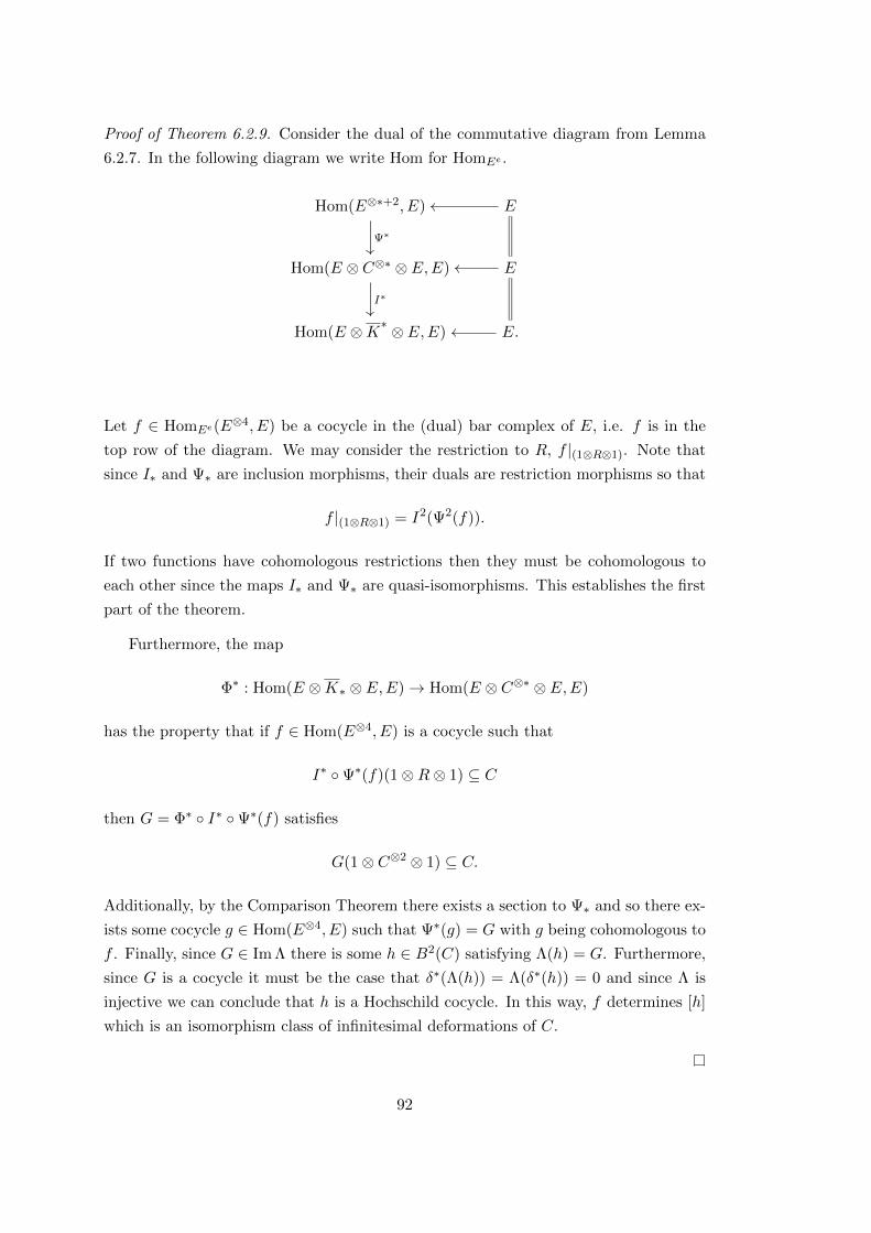
Proof of Theorem 6.2.9. Consider the dual of the commutative diagram from Lemma
6.2.7. In the following diagram we write Hom for HomEe .
Hom(E⊗∗+2, E) E
Hom(E ⊗ C⊗∗ ⊗ E,E) E
Hom(E ⊗K∗ ⊗ E,E) E.
Ψ∗
I∗
Let f ∈ HomEe(E⊗4, E) be a cocycle in the (dual) bar complex of E, i.e. f is in the
top row of the diagram. We may consider the restriction to R, f |(1⊗R⊗1). Note that
since I∗ and Ψ∗ are inclusion morphisms, their duals are restriction morphisms so that
f |(1⊗R⊗1) = I2(Ψ2(f)).
If two functions have cohomologous restrictions then they must be cohomologous to
each other since the maps I∗ and Ψ∗ are quasi-isomorphisms. This establishes the first
part of the theorem.
Furthermore, the map
Φ∗ : Hom(E ⊗K∗ ⊗ E,E)→ Hom(E ⊗ C⊗∗ ⊗ E,E)
has the property that if f ∈ Hom(E⊗4, E) is a cocycle such that
I∗ ◦Ψ∗(f)(1⊗R⊗ 1) ⊆ C
then G = Φ∗ ◦ I∗ ◦Ψ∗(f) satisfies
G(1⊗ C⊗2 ⊗ 1) ⊆ C.
Additionally, by the Comparison Theorem there exists a section to Ψ∗ and so there ex-
ists some cocycle g ∈ Hom(E⊗4, E) such that Ψ∗(g) = G with g being cohomologous to
f . Finally, since G ∈ Im Λ there is some h ∈ B2(C) satisfying Λ(h) = G. Furthermore,
since G is a cocycle it must be the case that δ∗(Λ(h)) = Λ(δ∗(h)) = 0 and since Λ is
injective we can conclude that h is a Hochschild cocycle. In this way, f determines [h]
which is an isomorphism class of infinitesimal deformations of C.
92
6.3 Overview of Calculations
In this section we describe a general procedure for applying Theorem 6.2.9 in the
context of families of deformations of Qgr(A) induced by automorphisms of minimal
rational surfaces. Since the procedure can be described in the abstract, we do so here.
In addition, we carry out some preliminary calculations that will be used in every case
considered in the rest of the chapter.
Recall from Section 6.1 the definition of σ : P1×P1 99K P1×P1. Recall further that
A is the subalgebra of D := K(u, v)[t : σ∗] generated by
E := {x1 := t, x2 := ut, x3 := vt, x4 := uvt}.
For any surface Y birational to P1 × P1, under b say, we get an induced birational self
map of Y given by σY := b ◦ σ ◦ b−1.
Since b is a birational map, we know by basic birational geometry (see [Har77,
Theorem 4.4]) that K(Y ) and K(P1 × P1) are isomorphic fields, with the pullback of b
defining an isomorphism, b∗, between them. Under this identification, σ∗Y is equal to
σ∗ as automorphisms of K(u, v).
Since we are interested in infinitesimal deformations of A, we consider a vector L
in the Lie algebra associated with Aut(Y ), which is a Lie group [DI09, Section 4]. By
considering a one-dimensional subspace of vectors {sL} we can apply the exponential
map and obtain a one-parameter subgroup of automorphisms τs = exp(sL).
As discussed in Section 6.1, such a τs defines a deformation of D and so we can
use Theorem 6.2.9 in order to test whether it actually corresponds to an infinitesimal
deformation of A. Write the deformed multiplication on D induced by τs as:
F (a, b) = ab+ F1(a, b)s+O(s2).
Recall that F1 is the infinitesimal of this deformation, and that it therefore satisfies
F1(a, b) =∂(F (a, b))
∂s
∣∣∣∣s=0
.
Theorem 6.2.9 implies that F induces an infinitesimal deformation of A if F1(R) ⊆A, where R = spK{ri|1 ≤ i ≤ 6} is given by the six relations:
r1 = x3x1 − x1x3, r2 = x2x4 − x4x2, r3 = x4x1 − x2x3,
r4 = x1x2 − x2x3, r5 = x3x2 − x1x4, r6 = x4x3 − x1x4.
As in Notation 3.2.1 we write a function f ∈ HH22(A) as a vector, with the ith compo-
nent being the image of ri under f . Since our algebra A is Koszul, the bar resolution
is quasi-isomorphic to the Koszul resolution and so these 6 images determine the coho-
93

mology class of the map f .
For any Y and L ∈ Lie(Aut(Y )), we can calculate the associated F1. We start by
setting τs := exp(sL) and defining U(s) := σ∗ ◦ τ∗s (u) and V (s) := σ∗ ◦ τ∗s (v), so that
in K(u, v)[[s]][t;σ∗ ◦ τ∗s ] we can write:
tv = V (s)t and tu = U(s)t.
Since τ0 = id we must have that U(0) = uv and V (0) = v. Then we calculate U ′(0) and
V ′(0). Once we have these derivatives we can use basic differentiation rules to calculate
F1. Since the following calculations are simple applications of the product rule we show
only the first in detail and record the rest in Appendix C.1.
F1(r1) =∂(F (r1))
∂s
∣∣∣∣s=0
=∂(F (x3x1 − x1x3))
∂s
∣∣∣∣s=0
=∂(vt2 − tvt)
∂s
∣∣∣∣s=0
=∂(vt2 − V (s)t2)
∂s
∣∣∣∣s=0
= −∂(V (s)t2)
∂s
∣∣∣∣s=0
= −V ′(0)t2.
The other calculations proceed along similar lines. We record the results in Table
6.1.
Relation r F1(r)
x3x1 − x1x3 −V ′(0)t2
x4x2 − x2x4 −u2vV ′(0)t2
x4x1 − x2x3 −uV ′(0)t2
x1x2 − x2x3 (U ′(0)− uV ′(0))t2
x3x2 − x1x4 −uvV ′(0)t2
x4x3 − x1x4 −vU ′(0)t2
Table 6.1: F1 Applied to the Relations of A
Now that this leg work is done, all it takes is to calculate the different values of
the functions in these formulae, and we get the relevant infinitesimals. So by Theorem
6.2.9, a sufficient condition for L to correspond to an infinitesimal deformation is for
each of the above six expressions to lie in A2. For example in the final row in Table 6.1
one must check that −vU ′(0)t2 is in the span of degree two monomials in the generators
of A.
Finally, we label the ordered basis of HH22(A) chosen in Section 3.3 by b1, . . . , b8.
Recall that this basis is
94

x1x3
0
0
x2x3
x1x4
0
x23
0
x1x4
0
0
x3x4
x21
0
0
x2x1
x2x3
0
0
x2x4
0
0
x1x4
0
0
x24
0
0
x3x4
0
0
x22
0
0
x2x3
0
0
0
0
x21
0
−x1x3
0
0
0
−x22
0
x2x4
6.4 Infinitesimals Arising from Automorphisms of P1× P1
In this case we have Y := X = P1 × P1 and b : X 99K X is the identity automorphism,
so that σY = σ. The automorphism group Aut(P1 × P1) is isomorphic to the wreath
product PGL2(K) oS2 [DI09, Section 4.3], however we only need to consider the identity
component. This component of Aut(P1 × P1) is isomorphic to PGL2×PGL2 which
means the associated Lie algebra is isomorphic to sl2× sl2. So for L we take M ×N ∈ sl2× sl2. This case is studied using very different methods in [RS12], where
the deformed algebras are analysed in their own right, rather than in terms of formal
deformation theory.
Take a matrix M ∈ sl2 and a formal deformation parameter s and consider
sM = s
(a b
c −a
).
Then clearly:
exp(sM) =
(1 + as bs
cs 1− as
)+O(s2),
and we get a similar formula for
N :=
(d e
f −d
).
In the following we omit all terms which have power of s greater than 1, since
this has no impact on the first order deformations and no impact on any derivatives
appearing.
Define τs = exp(sM, sN) so that:
τs([x : y][z : w]) = [(1 + as)x+ bsy : csx+ (1− as)y][(1 + ds)z+ esw : fsz+ (1− ds)w].
95
We have the formula
τs ◦ σ([x : y][z : w]) =
[(1 + as)xz + bsyw : csxz + (1− as)yw][(1 + ds)z + esw : fsz + (1− ds)w].
From this we can calculate U ′(0) by the following method:
U(s) = σ∗ ◦ τ∗s (u)
=(1 + as)xz + bsyw
csxz + (1− as)yw=
(1 + as)uv + bs
csuv + (1− as).
As a quick check on these calculations we note that U(0) = uv as required. In order to
calculate the derivative, let F be the numerator and G be the denominator. We have
the following:
F (0) = uv, F ′(0) = auv + b
G(0) = 1, G′(0) = cuv − a.
So that
U ′(0) =G(0)F ′(0)− F (0)G′(0)
G(0)2
= auv + b− uv(cuv − a)
= b− cu2v2 + 2auv
Likewise:
V (s) = σ∗ ◦ τ∗s (v) =(1 + ds)z + esw
fsz + (1− ds)w
=(1 + ds)v + es
fsv + (1− ds).
Note again this still makes some sense since V (0) = v. The derivative is somewhat
simpler to calculate in this case:
V ′(0) =∂
∂s
((1 + ds)v + es
vfs+ (1− ds)
)∣∣∣∣s=0
=(vfs+ (1− ds))(dv + e)− ((1 + ds)v + es)(vf − d)
(vfs+ (1− ds))2
∣∣∣∣s=0
= 2dv + e− fv2.
So putting this together with the calculations before, Table 6.2 records the images
96

of the relations under F1.
Relation Formula Image Under F1
r1 = x3x1 − x1x3 −V ′(0) (fv2 − 2dv − e)t2r2 = x2x4 − x4x2 −u2vV ′(0) (fu2v3 − eu2v − 2du2v2)t2
r3 = x4x1 − x2x3 −uV ′(0) (fuv2 − 2duv − eu)t2
r4 = x1x2 − x2x3 U ′(0)− uV ′(0) (b+ 2auv − cu2v2 − eu− 2duv + fuv2)t2
r5 = x3x2 − x1x4 −uvV ′(0) (fuv3 − euv − 2duv2)t2
r6 = x4x3 − x1x4 −vU ′(0) (cu2v3 − bv − 2auv2)t2
Table 6.2: Images of the Six Relations of A Under F1
Now we have the information necessary to check the admissibility of L. Recall that
this means we must check if each of the terms in the right hand column of this table
lies in
A2 = spK({uivjt2
∣∣0 ≤ i ≤ 2, 0 ≤ j ≤ 3}\ {v3t2, u2t2}
)(6.6)
= spK{x2x1, x22, x2x3, x2x4, x
21, x1x3, x1x4, x
23, x3x4, x
24}.
It is immediate by comparing the right hand column of Table 6.2 with (6.6) that
F1(ri) is always an element of A2. Therefore we can conclude that all of the directions
are admissible and so we do in fact get infinitesimal deformations of A with any choice
of L. In fact, the image of sl2× sl2 in HH2(A) coincides precisely with the unobstructed
component Vg from Theorem 5.3.2.
Theorem 6.4.1. All elements in sl2× sl2 are admissible. Furthermore, for any in-
finitesimal f ∈ Vg ⊆ HH22(A) there exists a one-parameter subgroup {τs} ⊆ Aut(P1×P1)
such that the associated infinitesimal deformation of A is isomorphic to f .
Proof. We have already shown that all elements are admissible. Identify sl2× sl2 with
K6 under the map :
((a b
c −a
),
(d e
f −d
))↔
a
b
c
d
e
f
.
From the right hand column of Table 6.2 we obtain a linear map Φ : sl2× sl2 → HH22(A)
97

represented by left multiplication by the matrix
A :=
0 0 0 −2x1x3 −x21 x2
3
0 0 0 −2x2x4 −x22 x2
4
0 0 0 −2x2x3 −x2x1 x1x4
2x2x3 x21 −x2x4 −2x2x3 −x2x1 x1x4
0 0 0 −2x1x4 −x2x3 x3x4
−2x1x4 −x1x3 x24 0 0 0
.
By referring to the basis of HH22(A) calculated in Chapter 3 (see Theorem 3.3.1) we
write the image of this map as an element of the vector space spanned by {b1, . . . , b8}.
Φ
((a b
c −a
),
(d e
f −d
))=
− 2d(b1 + b4) + f(b2 + b5)− e(b3 + b6) + bb7 + cb8 ∈ HH22(A). (6.7)
Note that in (6.7) we have written the cohomology classes of the columns of the matrix
A, which therefore may differ from the columns up to a coboundary. This is a vector
of the form∑aibi satisfying a1 = a4, a2 = a5 and a3 = a6. By Theorem 5.3.2 this is
precisely the defining equations of Vg. Furthermore, Φ is clearly surjective onto Vg.
Of course one notices that a is not present on the right hand side of equation (6.7),
which corresponds to the fact that this direction induces a trivial deformation. As a
check on our calculations we show this is indeed the case.
Lemma 6.4.2. Let
τ =
((a 0
0 a−1
),
(1 0
0 1
))∈ PGL2×PGL2,
then the subalgebra B of K(u, v)[t, t−1;σ∗ ◦ τ∗] generated by E is isomorphic to A.
Proof. We prove this be defining an explicit isomorphism φ : A→ B, given by
x1 7→ x1
x2 7→ x2
x3 7→ a2x3
x4 7→ a2x4
To see that φ is an isomorphism we note a few facts. Firstly, since σ∗ ◦τ∗(u) = a2uv
98
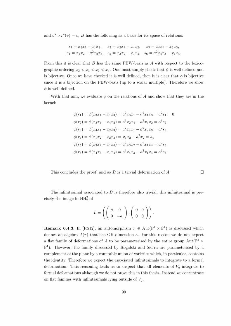
and σ∗ ◦ τ∗(v) = v, B has the following as a basis for its space of relations:
s1 = x3x1 − x1x3, s2 = x2x4 − x4x2, s3 = x4x1 − x2x3,
s4 = x1x2 − a2x2x3, s5 = x3x2 − x1x4, s6 = a2x4x3 − x1x4.
From this it is clear that B has the same PBW-basis as A with respect to the lexico-
graphic ordering x2 < x1 < x3 < x4. One must simply check that φ is well defined and
is bijective. Once we have checked it is well defined, then it is clear that φ is bijective
since it is a bijection on the PBW-basis (up to a scalar multiple). Therefore we show
φ is well defined.
With that aim, we evaluate φ on the relations of A and show that they are in the
kernel:
φ(r1) = φ(x3x1 − x1x3) = a2x3x1 − a2x1x3 = a2s1 = 0
φ(r2) = φ(x2x4 − x4x2) = a2x2x4 − a2x4x2 = a2s2
φ(r3) = φ(x4x1 − x2x3) = a2x4x1 − a2x2x3 = a2s3
φ(r4) = φ(x1x2 − x2x3) = x1x2 − a2x2 = s4
φ(r5) = φ(x3x2 − x1x4) = a2x3x2 − a2x1x4 = a2s5
φ(r6) = φ(x4x3 − x1x4) = a4x4x3 − a2x1x4 = a2s6.
This concludes the proof, and so B is a trivial deformation of A.
The infinitesimal associated to B is therefore also trivial; this infinitesimal is pre-
cisely the image in HH22 of
L =
((a 0
0 −a
),
(0 0
0 0
)).
Remark 6.4.3. In [RS12], an automorphism τ ∈ Aut(P1 × P1) is discussed which
defines an algebra A(τ) that has GK-dimension 3. For this reason we do not expect
a flat family of deformations of A to be parameterised by the entire group Aut(P1 ×P1). However, the family discussed by Rogalski and Sierra are parameterised by a
complement of the plane by a countable union of varieties which, in particular, contains
the identity. Therefore we expect the associated infinitesimals to integrate to a formal
deformation. This reasoning leads us to suspect that all elements of Vg integrate to
formal deformations although we do not prove this in this thesis. Instead we concentrate
on flat families with infinitesimals lying outside of Vg.
99

6.5 Infinitesimals Arising from Automorphisms of P2
We have seen that for every vector v in the variety Vg ⊂ HH22(A) we can find an
admissible direction L ∈ sl2× sl2 whose image under Φ is v. One might hope that
by considering automorphisms of other surfaces one might find admissible directions
whose images comprise Vu and Vq. In the following sections we show that this is not
the case, and that all admissible directions have images lying in Vg.
6.5.1 Calculating σP2
We recall some basic facts about P1×P1. Under the Segre embedding (see e.g. [EH00,
Section III.2.3]), we get an embedding of P1×P1 in P3. However, we change coordinates
slightly from the usual definition of the Segre embedding to ensure the formulae work
out nicely. We note here that this has no effect on the properties of the map, it is
purely a coordinate change. We define then:
S : P1 × P1 → P3, [x : y][z : w] 7→ [xw : xz : yw : yz].
This is an embedding of P1 × P1 into P3 as the quadric surface
Q := {[α : β : γ : δ] | αδ − βγ = 0},
where our rational coordinates are now u = α/γ and v = β/α. Now, if we take the
projection from [0 : 0 : 0 : 1] of this surface, we get dominant rational map, b−1, to
Y := P2. This map is given by
[α : β : γ : δ] 7→ [α : β : γ],
with birational inverse, b,
[α : β : γ] 7→ [α2 : αβ : αγ : βγ].
Now to transfer σ across to P2. Firstly we transfer it to Q, where it is simply the
composition:
[xw : xz : yw : yz] 7→ [x : y][z : w]
799K [xz : yw][z : w]
7→ [xwz : xz2 : yw2 : ywz] = [vxw : vxz : yw : yz],
which can be more neatly written as [α : β : γ : δ] 799K [βα : β2 : γα : δα].
100
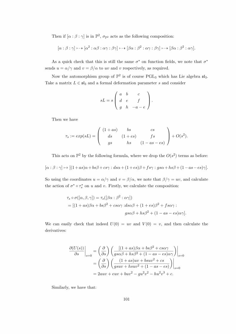
Then if [α : β : γ] is in P2, σP2 acts as the following composition:
[α : β : γ] 799K [α2 : αβ : αγ : βγ] 799K [βα : β2 : αγ : βγ] 799K [βα : β2 : αγ].
As a quick check that this is still the same σ∗ on function fields, we note that σ∗
sends u = α/γ and v = β/α to uv and v respectively, as required.
Now the automorphism group of P2 is of course PGL3 which has Lie algebra sl3.
Take a matrix L ∈ sl3 and a formal deformation parameter s and consider
sL = s
a b c
d e f
g h −a− e
.
Then we have
τs := exp(sL) =
(1 + as) bs cs
ds (1 + es) fs
gs hs (1− as− es)
+O(s2).
This acts on P2 by the following formula, where we drop the O(s2) terms as before:
[α : β : γ] 7→ [(1+as)α+ bsβ+ csγ : dsα+(1+es)β+fsγ : gsα+hsβ+(1−as−es)γ].
So using the coordinates u = α/γ and v = β/α, we note that β/γ = uv, and calculate
the action of σ∗ ◦ τ∗s on u and v. Firstly, we calculate the composition:
τs ◦ σ([α, β, γ]) = τs([βα : β2 : αγ])
= [(1 + as)βα+ bsβ2 + csαγ :dsαβ + (1 + es)β2 + fsαγ :
gsαβ + hsβ2 + (1− as− es)αγ].
We can easily check that indeed U(0) = uv and V (0) = v, and then calculate the
derivatives:
∂(U(s))
∂s
∣∣∣∣s=0
=
(∂
∂s
)([(1 + as)βα+ bsβ2 + csαγ
gsαβ + hsβ2 + (1− as− es)αγ
)∣∣∣∣s=0
=
(∂
∂s
)((1 + as)uv + bsuv2 + cs
gsuv + hsuv2 + (1− as− es)
)∣∣∣∣s=0
= 2auv + euv + buv2 − gu2v2 − hu2v3 + c.
Similarly, we have that:
101

∂(V (s))
∂s
∣∣∣∣s=0
=
(∂
∂s
)(dsαβ + (1 + es)β2 + fsαγ
(1 + as)βα+ bsβ2 + csαγ
)∣∣∣∣s=0
=
(∂
∂s
)(dsuv + (1 + es)uv2 + fs
(1 + as)uv + bsuv2 + cs
)∣∣∣∣s=0
= d+ ev + fu−1v−1 − av − bv2 − cu−1.
We can see already that to be able to apply Theorem 6.2.9, f and c will both have to
be 0. This is because F1(r1) = −V ′(0) and if these are not zero then V ′(0)t2 will not
be an element of A2 as required. Likewise, h must be 0 since −vU ′(0)t2 must be in
A2 (equation 6 in Section 6.3) and this would contain the term hu2v4t2, which has a
power of v that is too high for this to lie in A2.
After setting f = c = h = 0, we record this data in Table 6.3 for ease of reading.
Relation Formula Image Under F1
x3x1 − x1x3 −V ′(0) (bv2 + av − ev − d)t2
x2x4 − x4x2 −u2vV ′(0) (bu2v3 + au2v2 − eu2v2 − du2v)t2
x4x1 − x2x3 −uV ′(0) (buv2 + auv − euv − du)t2
x1x2 − x2x3 U ′(0)− uV ′(0) (−gu2v2 + 2buv2 + 3auv − du)t2
x3x2 − x1x4 −uvV ′(0) (buv3 + auv2 − euv2 − duv)t2
x4x3 − x1x4 −vU ′(0) (gu2v3 − 2auv2 − euv2 − buv3)t2
Table 6.3: Images of the Six Relations of A under F1
Theorem 6.5.1. Let Φ be the map from admissible directions to HH22(A) determined
by the deformations induced by τs. Every admissible direction in sl3 is sent under Φ to
an infinitesimal deformation lying in Vg. Furthermore, the image of these directions is
a four dimensional subspace of Vg.
Proof. We embed the space of admissible directions in sl3 into K5 using the mapping
a b 0
d e 0
g 0 −a− e
↔
a
b
d
e
g
.
102
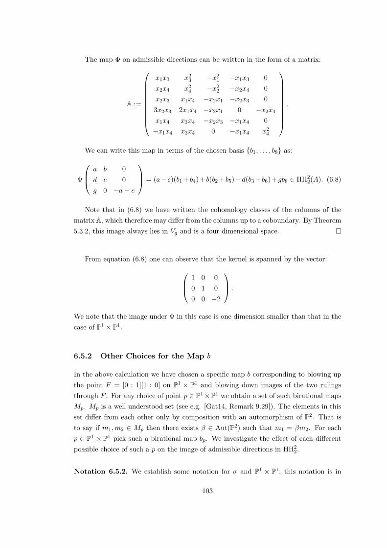
The map Φ on admissible directions can be written in the form of a matrix:
A :=
x1x3 x23 −x2
1 −x1x3 0
x2x4 x24 −x2
2 −x2x4 0
x2x3 x1x4 −x2x1 −x2x3 0
3x2x3 2x1x4 −x2x1 0 −x2x4
x1x4 x3x4 −x2x3 −x1x4 0
−x1x4 x3x4 0 −x1x4 x24
.
We can write this map in terms of the chosen basis {b1, . . . , b8} as:
Φ
a b 0
d e 0
g 0 −a− e
= (a−e)(b1 + b4)+ b(b2 + b5)−d(b3 + b6)+gb8 ∈ HH22(A). (6.8)
Note that in (6.8) we have written the cohomology classes of the columns of the
matrix A, which therefore may differ from the columns up to a coboundary. By Theorem
5.3.2, this image always lies in Vg and is a four dimensional space.
From equation (6.8) one can observe that the kernel is spanned by the vector: 1 0 0
0 1 0
0 0 −2
.
We note that the image under Φ in this case is one dimension smaller than that in the
case of P1 × P1.
6.5.2 Other Choices for the Map b
In the above calculation we have chosen a specific map b corresponding to blowing up
the point F = [0 : 1][1 : 0] on P1 × P1 and blowing down images of the two rulings
through F . For any choice of point p ∈ P1×P1 we obtain a set of such birational maps
Mp. Mp is a well understood set (see e.g. [Gat14, Remark 9.29]). The elements in this
set differ from each other only by composition with an automorphism of P2. That is
to say if m1,m2 ∈ Mp then there exists β ∈ Aut(P2) such that m1 = βm2. For each
p ∈ P1 × P1 pick such a birational map bp. We investigate the effect of each different
possible choice of such a p on the image of admissible directions in HH22.
Notation 6.5.2. We establish some notation for σ and P1 × P1; this notation is in
103
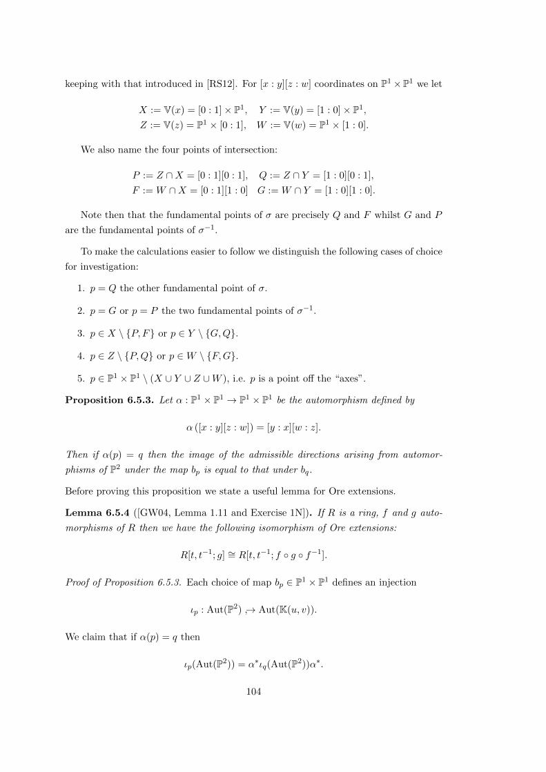
keeping with that introduced in [RS12]. For [x : y][z : w] coordinates on P1×P1 we let
X := V(x) = [0 : 1]× P1, Y := V(y) = [1 : 0]× P1,
Z := V(z) = P1 × [0 : 1], W := V(w) = P1 × [1 : 0].
We also name the four points of intersection:
P := Z ∩X = [0 : 1][0 : 1], Q := Z ∩ Y = [1 : 0][0 : 1],
F := W ∩X = [0 : 1][1 : 0] G := W ∩ Y = [1 : 0][1 : 0].
Note then that the fundamental points of σ are precisely Q and F whilst G and P
are the fundamental points of σ−1.
To make the calculations easier to follow we distinguish the following cases of choice
for investigation:
1. p = Q the other fundamental point of σ.
2. p = G or p = P the two fundamental points of σ−1.
3. p ∈ X \ {P, F} or p ∈ Y \ {G,Q}.
4. p ∈ Z \ {P,Q} or p ∈W \ {F,G}.
5. p ∈ P1 × P1 \ (X ∪ Y ∪ Z ∪W ), i.e. p is a point off the “axes”.
Proposition 6.5.3. Let α : P1 × P1 → P1 × P1 be the automorphism defined by
α ([x : y][z : w]) = [y : x][w : z].
Then if α(p) = q then the image of the admissible directions arising from automor-
phisms of P2 under the map bp is equal to that under bq.
Before proving this proposition we state a useful lemma for Ore extensions.
Lemma 6.5.4 ([GW04, Lemma 1.11 and Exercise 1N]). If R is a ring, f and g auto-
morphisms of R then we have the following isomorphism of Ore extensions:
R[t, t−1; g] ∼= R[t, t−1; f ◦ g ◦ f−1].
Proof of Proposition 6.5.3. Each choice of map bp ∈ P1 × P1 defines an injection
ιp : Aut(P2) ↪→ Aut(K(u, v)).
We claim that if α(p) = q then
ιp(Aut(P2)) = α∗ιq(Aut(P2))α∗.
104
Since α(p) = q, we know that bpα is a birational map with unique fundamental
point q. It follows that bpα ∈ Mq, and so there exists an automorphism β ∈ Aut(P2)
satisfying
βbq = bpα.
In particular bpαb−1q = β is an automorphism of P2 and for f ∈ Aut(P2) we have
ιp(β−1fβ) = α∗ιq(f)α∗.
The claim follows immediately.
Therefore, if τ∗s is some family of automorphisms arising from the choice of coordi-
nates from bp, then there exists some family ρ∗s arising from the choice of coordinates
from bq such that:
τ∗s = α∗ρ∗sα∗.
Note that since α is an involution, (α∗)−1 = α∗. Furthermore,
α∗σ∗α∗ = σ∗.
Therefore, applying Lemma 6.5.4 we have the isomorphism
K(u, v)[t, t−1;σ∗ ◦ τ∗s ] = K(u, v)[t, t−1;σ∗ ◦ α∗ ◦ ρ∗s ◦ α∗]
= K(u, v)[t, t−1;α∗ ◦ σ∗ ◦ ρ∗s ◦ α∗]∼= K(u, v)[t, t−1;σ∗ ◦ ρ∗s].
In other words any infinitesimal deformation arising from studying bq will also arise
from studying bp, and so the associated spaces of infinitesimal deformations will are
equal.
By Proposition 6.5.3, in Cases 2, 3 and 4 we only need consider one of the two
possible options. Furthermore, this proposition means that we have already considered
Case 1 in the preceding work of Section 6.5.1.
We elaborate here on the final case in detail. The details of the calculations for the
other cases can be found in Appendix C.2, whereas the results are recorded in Table
6.4 at the end of this section.
Case 5
In this case p ∈ P1 × P1 \ (X ∪ Y ∪ Z ∪W ), i.e. p is a point away from the four ‘axes’.
Choosing a point to blow up is equivalent to choosing a point on Q to project from.
We use the coordinates [A : B : C] on P2, [α : β : γ : δ] for coordinates on P3 (in which
105

Q is embedded) and [x : y][z : w] as coordinates for P1 × P1. We will use the same τs
as before, defined by:
τs :=
(1 + as) bs cs
ds (1 + es) fs
gs hs (1− as− es)
+O(s2).
We also point out that in order for an element of the Lie algebra to be inadmissible
we need to find terms that do not lie in A. We can determine these terms simply by
observing the powers of u and v appearing in U ′(0) and V ′(0).
If p ∈ P1×P1 \ (X ∪Y ∪Z ∪W ) then we can write it as p = [1 : M ][1 : N ] for some
M,N ∈ K∗. This corresponds to the point [N : 1 : MN : M ] on Q and so we project
from this point.
This is then the map [α : β : γ : δ] 799K [α−Nβ : γ −MNβ : δ −Mβ]. Composing
this with the Segre embedding gives us the map:
bp : [x : y][z : w] 799K [xw −Nxz : yw −MNxz : yz −Mxz].
Note that since
b−1p : [A,B,C] 799K [A : B −NC][C : B −MA],
this map induces u = AB−NC and v = C
B−MA as coordinates on P2. Therefore σP2 is the
following composition:
σP2 : [A : B;C] 799K [A : B −NC][C : B −MA]
7 σ99K [AC : (B −NC)(B −MA)][C : B −MA]
799K [AC(B −MA)−NAC2 : (B −NC)(B −MA)2 −MNAC2 :
(B −NC)(B −MA)C −MAC2].
We note that
u 7→ AC(B −MA)−NAC2
(B −NC)(B −MA)2 −MNAC2 −N(B −NC)(B −MA)C +MNAC2
= (A
B −NC)(
C
B −MA) = uv,
and
v 7→ (B −NC)(B −MA)C −MAC2
(B −NC)(B −MA)2 −MNAC2 −MAC(B −MA) +MNAC2
=C
B −MA= v.
106
We record the following formulae which are easily derivable from the above:
C
B=
Muv − vMNuv − i
,A
B=
Nuv − uMNuv − 1
.
Then σ∗ ◦ τ∗s has the following effect (up to degree 1) on v:
uτ∗s7−→ (1 + as)A+ bsB + csC
dsA+ (1 + es)B + fsC −N(gsA+ hsB + (1− as− es)C)
=(1 + as)(Nuv − u) + bs(MNuv − 1) + cs(Muv − v)
χ(s)
where
χ(s) = ds(Nuv − u) + (1 + es)(MNuv − 1) + fs(Muv − v)−
N(gs(Nuv − u) + hs(MNuv − 1) + (1− as− es)(Muv − v)).
Under σ this is sent to F (s)/G(s) where:
F (s) = (1 + as)(Nuv2 − uv) + bs(MNuv2 − 1) + cs(Muv2 − v),
and
G(s) = ds(Nuv2 − uv) + (1 + es)(MNuv2 − 1) + fs(Muv2 − v)−
N(gs(Nuv2 − uv) + hs(MNuv2 − 1) + (1− as− es)(Muv2 − v)).
In preparation for using the quotient rule to differentiate this we calculate some inter-
mediate values.
F (0) = Nuv2 − uv, F ′(0) = a(Nuv2 − uv) + b(MNuv2 − 1) + c(Muv2 − v),
G(0) = NV − 1, G′(0) = d(Nuv2 − uv) + e(MNuv2 − 1) + f(Muv2 − v)−
N(g(Nuv2 − uv)− h(MNuv2 − 1) + (a+ e)M(uv2 − v).
107
Applying these formula gives us the following result:
∂s(σ∗ ◦ τ∗s (u))|s=0 = auv + aNuv
Muv2 − vNv − 1
+ bMNuv − 1
Nv − 1+ c
Muv2 − vNv − 1
− du2v2
− fuvMuv − vNv − 1
−Nguv −NhuvMNuv2 − 1
Nv − 1
+ eNuvMuv2 − vNv − 1
− euvMNuv2 − 1
Nv − 1.
Then because of the denominators appearing above, we must have that a = b =
c = f = h = 0 in order for this to be admissible.
Turning then to the calculation with respect to v:
vτ∗s7−→ gsA+ hsB + (1− as− es)C
dsA+ (1 + es)B + fsC −M((1 + as)A+ bsB + csC)
=gsA+ (1− es)C
dsA+ (1 + es)B −MA
=gs(Nuv − u) + (1− es)(Muv − v)
ds(Nuv − u) + (1 + es)(MNuv − 1)−M(Nuv − u)
σ7−→ gs(Nuv2 − uv) + (1− es)(Muv2 − v)
ds(Nuv2 − uv) + (1 + es)(MNuv2 − 1)−M(Nuv2 − uv)
Which has the following derivative:
∂s(σ∗ ◦ τ∗s (v))|s=0 = g
Nuv2 − uvMuv − 1
− e(Muv − v)(Muv +MNuv2 − 1)
(Muv − 1)2
− d(Muv − v)(Nuv2 − uv)
(Muv − 1)2
Similarly to above, just by looking at the denominators one can see that no cancellation
will occur here and indeed it is required that e, d and g are all 0 for this to be an
admissible direction. Therefore in this case the image of the admissible direction is the
trivial deformation.
Conclusion
The results of the calculations above (and those in Appendix C.2) are recorded in Table
6.4.
108

Case Dimension of Image in HH22
1) p = Q 4
2) p := G or p = P 4
3) p ∈ X \ {P, F} or p ∈ Y \ {G,Q} 0
4)p ∈ Z \ {P,Q} or p ∈W \ {F,G} 1
5)p ∈ P1 × P1 \ (X ∪ Y ∪ Z ∪W ) 0
Table 6.4: Dimension of the Image of the Admissible Directions for other choices of b
We can summarise the results in the following proposition.
Proposition 6.5.5. For any choice of point p ∈ P1×P1 and birational map bp, the set
of admissible directions in sl3 is sent under Φ to infinitesimal deformations of A lying
in Vg.
6.6 Infinitesimals Arising from Automorphisms of Fn
In this section we turn to the higher Hirzebruch surfaces. We follow the procedure of
Section 6.3 and choose a birational map b : P1×P1 → Fn. Since we found in Proposition
6.5.5 and Table 6.4 that the best choice of b was one that blows one of the fundamental
points of σ we only consider one such map in this section. We take Proposition 6.5.5
as evidence that this will not reduce the space of infinitesimals we come across.
6.6.1 Calculating σFn
In what follows we assume n ≥ 2.
Recall that a Hirzebruch surface, denoted Fn, is the projective variety given as a
subvariety of Pn+3 by:
Fn =
{[x0 : x1 : . . . : xn+1 : y0 : y1]
∣∣∣∣∣ rank
(x0 x1 . . . xn y0
x1 x2 . . . xn+1 y1
)= 1
}.
We first wish to calculate σFn . There is a natural map from Fn to Q, the embedding
of P1 × P1 into P3 as a quadric surface. Since rank
(x0 x1 . . . xn y0
x1 x2 . . . xn+1 y1
)= 1,
this implies that the minor
(x0 y0
x1 y1
)has determinant 0. This means that:
[x0 : x1 : . . . : y1] 799K [x0 : x1 : y0 : y1].
is a birational map Fn 99K Q, and so we can use this to transfer σ. We note that the
requirement on the rank of the matrix is equivalent to the fact that the ratio from x0
to x1 is the same as the ratio from xi to xi+1. This allows us to define the inverse
109
birational map as:
[x0 : x1 : y0 : y1] 799K [x0 : x1 : x21/x0 : x3
1/x20 : . . . : y0 : y1].
We can now calculate σFn as the following composition:
[x0 : x1 : . . . : y1] 799K [x0 : x1 : y0 : y1] 799K [x1 : x21/x0 : y0 : y1] 799K [x1 : x2
1/x0 : x31/x
20 . . . : y1],
or more simply:
[x0 : x1 : . . . : y1] 799K [x1 : x2 : . . . : xn+1 : xn+1x1
x0: y0 : y1].
As a check on these calculations we verify that v = x1/x0 gets sent to (x21x0
) 1x1
= v and
that u = x0/y0 gets sent to x1y0
= x1x0
x0y0
= uv as required.
6.6.2 Automorphisms of Fn for n ≥ 2
Firstly we recall some definitions, and then relate these to the Hirzebruch surfaces. The
weighted projective space P(1, 1, n) is defined similarly to P2, in that it is a quotient
of K3. However, the equivalence relation is slightly different, in that for any nonzero
λ ∈ K(x, y, z) ∼ (λx, λy, λnz).
In order to make it clear what kind of space a point is in, we write [a, b, c] for a point
in P(1, 1, n) and [a : b : c] for a point in P2. It is well known (e.g. [Dol82, Section
1.2.3]) that Fn is the blow up of P(1, 1, n) at the unique singular point p := [0, 0, 1].
The following is well known to experts but we have not found a reference for it so we
prove it here.
Lemma 6.6.1. Let X be a projective surface with a unique singular point, p, and X
the blow up at this point, such that X has a unique divisor of self-intersection −n whose
image under the blow up map is p. Then there is an isomorphism between Aut(X) and
Aut(X) induced by the blow up map.
Proof. Let π : X → X be the blow up map and consider α ∈ Aut(X). Since p is
the unique singular point of X, it must be the case that α fixes p. By the universal
property of blow ups [Har77, Proposition 7.14] we know that there is a unique morphism
α : X → X such that π ◦ α = α ◦ π. The same reasoning applies to α−1, which means
we have a morphism α ◦ (α−1) which satisfies:
π ◦ α ◦ (α−1) = α ◦ α−1 ◦ π = 1 ◦ π.
The universal property means that α ◦ (α−1) is unique, so that it must be the identity.
110
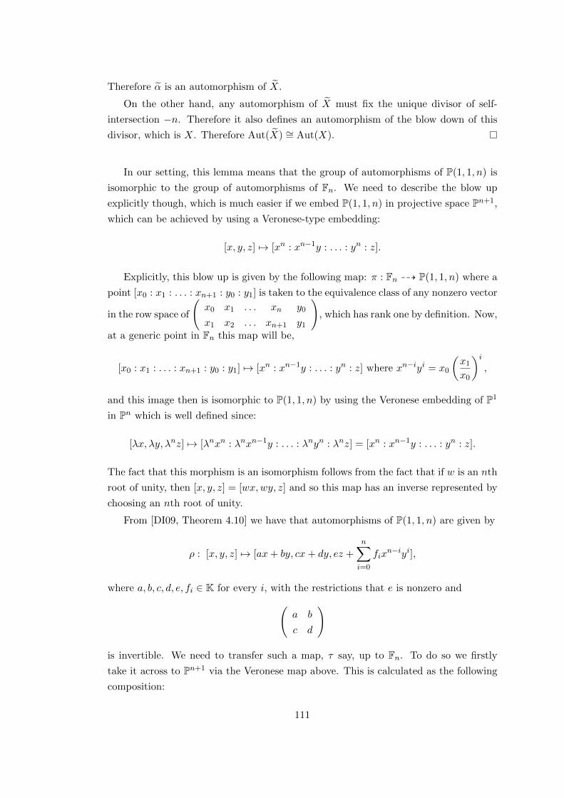
Therefore α is an automorphism of X.
On the other hand, any automorphism of X must fix the unique divisor of self-
intersection −n. Therefore it also defines an automorphism of the blow down of this
divisor, which is X. Therefore Aut(X) ∼= Aut(X).
In our setting, this lemma means that the group of automorphisms of P(1, 1, n) is
isomorphic to the group of automorphisms of Fn. We need to describe the blow up
explicitly though, which is much easier if we embed P(1, 1, n) in projective space Pn+1,
which can be achieved by using a Veronese-type embedding:
[x, y, z] 7→ [xn : xn−1y : . . . : yn : z].
Explicitly, this blow up is given by the following map: π : Fn 99K P(1, 1, n) where a
point [x0 : x1 : . . . : xn+1 : y0 : y1] is taken to the equivalence class of any nonzero vector
in the row space of
(x0 x1 . . . xn y0
x1 x2 . . . xn+1 y1
), which has rank one by definition. Now,
at a generic point in Fn this map will be,
[x0 : x1 : . . . : xn+1 : y0 : y1] 7→ [xn : xn−1y : . . . : yn : z] where xn−iyi = x0
(x1
x0
)i,
and this image then is isomorphic to P(1, 1, n) by using the Veronese embedding of P1
in Pn which is well defined since:
[λx, λy, λnz] 7→ [λnxn : λnxn−1y : . . . : λnyn : λnz] = [xn : xn−1y : . . . : yn : z].
The fact that this morphism is an isomorphism follows from the fact that if w is an nth
root of unity, then [x, y, z] = [wx,wy, z] and so this map has an inverse represented by
choosing an nth root of unity.
From [DI09, Theorem 4.10] we have that automorphisms of P(1, 1, n) are given by
ρ : [x, y, z] 7→ [ax+ by, cx+ dy, ez +
n∑i=0
fixn−iyi],
where a, b, c, d, e, fi ∈ K for every i, with the restrictions that e is nonzero and(a b
c d
)
is invertible. We need to transfer such a map, τ say, up to Fn. To do so we firstly
take it across to Pn+1 via the Veronese map above. This is calculated as the following
composition:
111

[xn : xn−1y : . . . : yn : z] 7→ [x, y, z] 7→ [ax+ by, cx+ dy, ez +
n∑i=0
fixn−iyi]
7→ [(ax+ by)n : (cx+ dy)(ax+ by)n−1 : . . . : (cx+ dy)n : ez +∑i
fixn−iyi].
For ease of reading we set Ai := (cx + dy)i(ax + by)n−i for i from 1 to n and
An+1 := ey0 +∑fix
n−iyi. Then we can transfer this back up to Fn by using the blow
up map. If we take a point [x0 : . . . : xn+1 : y0 : y1] and act on it by σ then we get
the point [x1 : x2 . . . : xn+1x1x0
: y0 : y1]. We assume we are in the open set where x0 is
nonzero, then in the above equations we choose x and y so that
xn−iyi = x0
(x1
x0
)i+1
.
This means that under τ this point is sent to:
τ ◦ σ[x0 : . . . : xn+1 : y0 : y1] = [A0 : A1 : . . . : AnA1
A0: An+1 : An+1
A1
A0].
Now, the identity automorphism in this situation corresponds to setting
(a, b, c, d, e, f0, . . . , fn) := (1, 0, 0, 1, 1, 0, . . . , 0),
so that perturbing in one direction with parameter s corresponds to a choice of auto-
morphism given by (1+as, bs, cs, 1+ds, 1+es, sf0, . . . , sfn). This gives us the following
formulae for U(s) and V (s):
U(s) =A0
An+1
=((1 + as)x+ bsy)n
(1 + es)y0 +∑n
i fixn−iyi
and
V (s) =A1
A0
=(csx+ (1 + ds)y)((1 + as)x+ bsy)n−1
((1 + as)x+ bsy)n.
112

Taking each in turn, we have the following:
V (0) =yxn−1
xn
=uv2
uv= v.
As for the derivative, we start by multiplying top and bottom by 1/y0 so that everything
is in terms of u’s and v’s. The numerator has a derivative at zero of:
cuv + duv2 + (n− 1)auv2 + (n− 1)buv3,
whereas the denominator has derivative:
nauv + nbuv2.
This then implies a derivative of:
V ′(0) =uv(cuv + duv2 + (n− 1)auv2 + (n− 1)buv3)− uv2(nauv + nbuv2)
(uv)2
= c+ dv − av − bv2.
Likewise we can calculate U ′(0) in a similar fashion. The derivative of the numerator
at zero is
nauv + nbuv2
and of the denominator is:
e+∑
fiuvi+1,
which gives a derivative of:
nauv + nbuv2 − euv −n∑i
fiu2vi+2.
We can now consider the admissibility of L. Since −vU ′(0)t2 will contain the terms∑i fiu
2vi+3t2, for this to be admissible we certainly need fi = 0 for any i greater than
0, since no powers of v higher than 3 appear in A2. These are the only restrictions on
admissibility. For this reason we write f for f0 and record the results in Table 6.5.
113
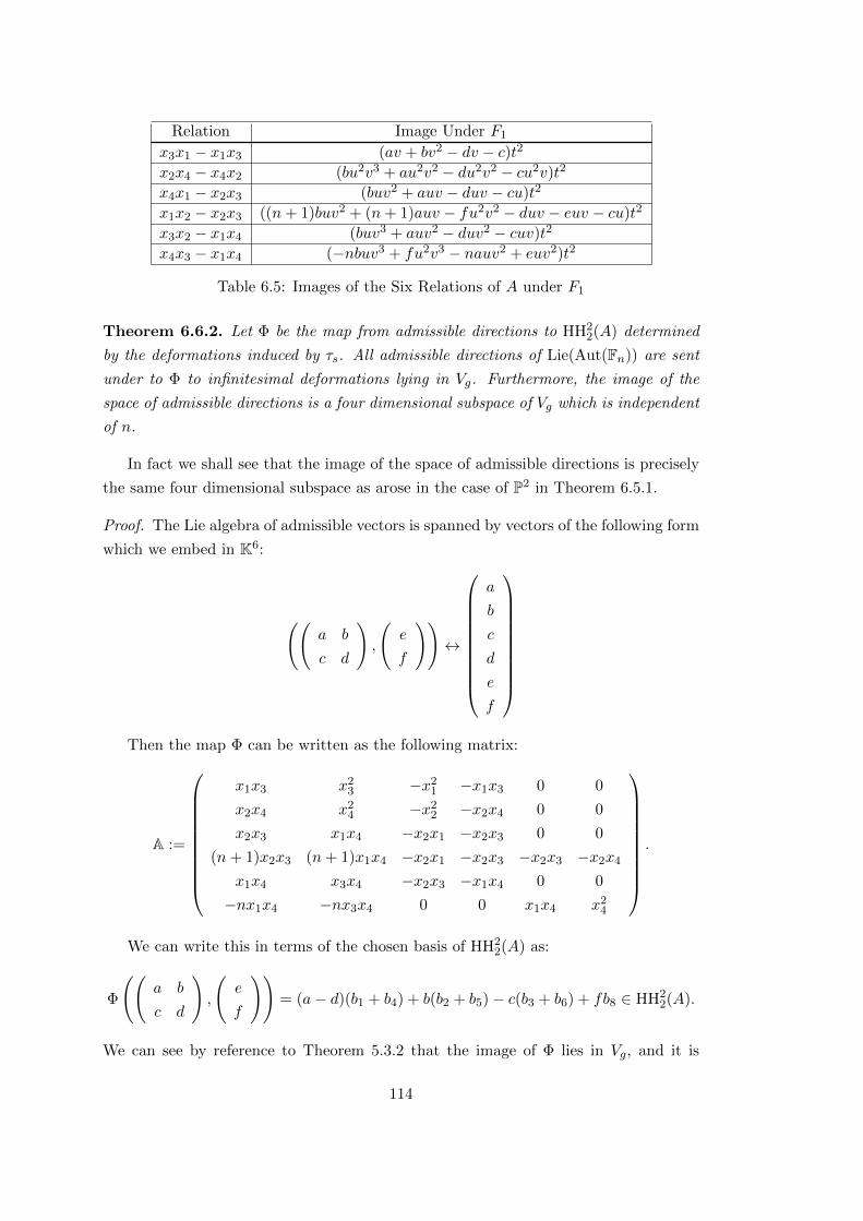
Relation Image Under F1
x3x1 − x1x3 (av + bv2 − dv − c)t2x2x4 − x4x2 (bu2v3 + au2v2 − du2v2 − cu2v)t2
x4x1 − x2x3 (buv2 + auv − duv − cu)t2
x1x2 − x2x3 ((n+ 1)buv2 + (n+ 1)auv − fu2v2 − duv − euv − cu)t2
x3x2 − x1x4 (buv3 + auv2 − duv2 − cuv)t2
x4x3 − x1x4 (−nbuv3 + fu2v3 − nauv2 + euv2)t2
Table 6.5: Images of the Six Relations of A under F1
Theorem 6.6.2. Let Φ be the map from admissible directions to HH22(A) determined
by the deformations induced by τs. All admissible directions of Lie(Aut(Fn)) are sent
under to Φ to infinitesimal deformations lying in Vg. Furthermore, the image of the
space of admissible directions is a four dimensional subspace of Vg which is independent
of n.
In fact we shall see that the image of the space of admissible directions is precisely
the same four dimensional subspace as arose in the case of P2 in Theorem 6.5.1.
Proof. The Lie algebra of admissible vectors is spanned by vectors of the following form
which we embed in K6:
((a b
c d
),
(e
f
))↔
a
b
c
d
e
f
Then the map Φ can be written as the following matrix:
A :=
x1x3 x23 −x2
1 −x1x3 0 0
x2x4 x24 −x2
2 −x2x4 0 0
x2x3 x1x4 −x2x1 −x2x3 0 0
(n+ 1)x2x3 (n+ 1)x1x4 −x2x1 −x2x3 −x2x3 −x2x4
x1x4 x3x4 −x2x3 −x1x4 0 0
−nx1x4 −nx3x4 0 0 x1x4 x24
.
We can write this in terms of the chosen basis of HH22(A) as:
Φ
((a b
c d
),
(e
f
))= (a− d)(b1 + b4) + b(b2 + b5)− c(b3 + b6) + fb8 ∈ HH2
2(A).
We can see by reference to Theorem 5.3.2 that the image of Φ lies in Vg, and it is
114
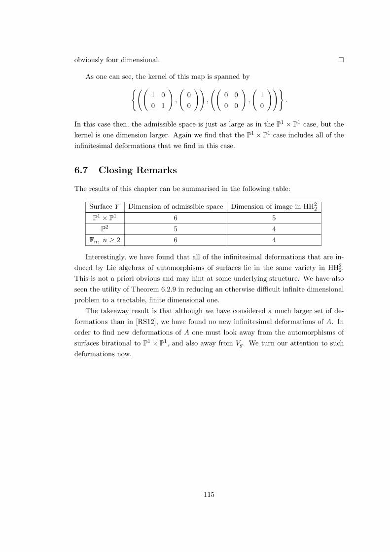
obviously four dimensional.
As one can see, the kernel of this map is spanned by{((1 0
0 1
),
(0
0
)),
((0 0
0 0
),
(1
0
))}.
In this case then, the admissible space is just as large as in the P1 × P1 case, but the
kernel is one dimension larger. Again we find that the P1 × P1 case includes all of the
infinitesimal deformations that we find in this case.
6.7 Closing Remarks
The results of this chapter can be summarised in the following table:
Surface Y Dimension of admissible space Dimension of image in HH22
P1 × P1 6 5
P2 5 4
Fn, n ≥ 2 6 4
Interestingly, we have found that all of the infinitesimal deformations that are in-
duced by Lie algebras of automorphisms of surfaces lie in the same variety in HH22.
This is not a priori obvious and may hint at some underlying structure. We have also
seen the utility of Theorem 6.2.9 in reducing an otherwise difficult infinite dimensional
problem to a tractable, finite dimensional one.
The takeaway result is that although we have considered a much larger set of de-
formations than in [RS12], we have found no new infinitesimal deformations of A. In
order to find new deformations of A one must look away from the automorphisms of
surfaces birational to P1 × P1, and also away from Vg. We turn our attention to such
deformations now.
115

116
Chapter 7
Deformations of Aq Arising from
Quantum Analogues of
Geometric Automorphisms
7.1 Introduction
In this chapter we examine the infinitesimal deformations of the algebra Aq and relate
these back to deformations of A. We do this by mimicking the work on geometric
automorphisms of K(u, v) (see Chapter 6) but in the context of Aq. Recall from Section
3.4 that σ ∈ Aut(Kq(u, v)) is the automorphism defined by
σ(u) = uv and σ(v) = v.
Then in this chapter we wish to study deformations of
Qgr(Aq) = Kq(u, v)[t, t−1;σ]
which arise from quantum analogues of geometric automorphisms of K(u, v).
The automorphism group of Kq(u, v) is in general not well understood (see e.g.
[AC99] or [Fry14]). However, Alev and Dumas [AD95] have carried out a study of
subgroups of automorphisms of Kq(u, v) that correspond precisely to ‘quantised’ auto-
morphisms of K(u, v). For this reason we discuss this paper at length in Section 7.2
before applying their work in Section 7.3.
We find that these deformations correspond to a four dimensional space of infinites-
imal deformations of Aq. Since by Theorem 3.4.3 HH22(Aq) is four dimensional, these
deformations have infinitesimals that comprises all of HH22(Aq). Furthermore, taking
the semi-classical limit q → 1 we obtain a 2 dimensional space of infinitesimal defor-
mations of the algebra A which lies in the set Vq (see Section 5.3).
117

7.2 A Discussion of a Paper of Alev and Dumas
Any definitions and propositions from this section are taken directly from [AD95]. This
paper is written in French and we have translated any quoted material here. For this
reason we do not include citations for every proposition and definition for this section.
7.2.1 Overview
The paper [AD95] is an examination of the automorphism group of a few skew fields of
interest. The relevant portions of the paper concern Kq(u, v), the division ring of the
quantum plane Kq[u, v]. We discuss their results here as we wish to apply them in the
context of the algebra Aq.
The main idea of the work is to quantise the structure of the Cremona group. Two
subgroups of the Cremona group are singled out in particular. Following from this,
quantum analogues of those subgroups are identified in the quantum Cremona group.
Definition 7.2.1. The quantum Cremona group is the group of automorphisms of the
division ring Kq(u, v).
7.2.2 Subgroups of the Classical Cremona Group
We have already come across several subgroups of the Cremona group in Chapter
6. Alev and Dumas bring particular attention to one of the subgroups appearing in
Chapter 6: the automorphism group of P2.
Definition 7.2.2. We define Z to be the subgroup of Aut(K(u, v)) isomorphic to
PGL3(K) where a matrix
M :=
a b c
d e f
g h i
acts by
M(u) =au+ bv + c
gu+ hv + iand M(v) =
du+ ev + f
gu+ hv + i.
Alev and Dumas also draw attention to a second subgroup of the Cremona group,
which we have not considered before, although it contains the identity component of
Aut(P1 × P1).
Definition 7.2.3. For any
(α γ
β δ
)∈ GL2(K) and
(a(u) c(u)
b(u) d(u)
)∈ GL2(K(u))
we define an automorphism θ ∈ Aut(K(u, v)) by
θ(v) =a(u)v + b(u)
c(u)v + d(u)and θ(u) =
αu+ β
γu+ δ.
118

These automorphisms form a subgroup of Aut(K(u, v)) which we refer to as Y . Note
that Y is precisely the subgroup of automorphisms θ of K(u, v) that satisfy
θ(K(u)) = K(u).
7.2.3 Subgroups of the Quantum Cremona Group
We now turn our attention to the quantum analogues of the above groups.
Definition 7.2.4. For any
(a c
b d
)∈ SL(2,Z) and (α, β) ∈ (K∗)2 we define an
automorphism ψ of Kq(u, v) by
ψ(v) = αubva and ψ(u) = βudvc.
Automorphisms defined in this manner form a subgroup of Aut(Kq(u, v)), which we
call H.
Note that by Proposition 1.6 of [AD96], this group is precisely the extension to
Kq(u, v) of the automorphism group of the quantum torus Kq[u±1, v±1].
Alev and Dumas show that there is a subgroup of H which is the quantum analogue
of Z ∼= PGL3(K).
Proposition 7.2.5. [AD95, Proposition 1.5] Let C ≤ H be the subgroup of those
automorphisms whose defining matrix
(a c
b d
)∈ SL(2,Z) lies in the cyclic subgroup
generated by
(0 1
−1 −1
). Then C is the subgroup of Aut(Kq(u, v)) of elements θ
such that
θ(v) = UW−1 and θ(u) = VW−1,
with U, V,W ∈ Kq[u, v] nonzero elements of degree at most one.
Definition 7.2.6. For α ∈ K∗ and f ∈ K(u)∗ we define an automorphism µ ∈Aut(Kq(u, v)) by
µ(u) = αu and µ(v) = f(u)v.
These automorphisms form a group which we call B+. Likewise we define B− to be
the group of automorphisms of the form
λ(u) = ug(v) and λ(v) = βv
for some β ∈ K∗ and g ∈ K(v)∗.
Let ω be the involution defined by ω(u) = u−1 and ω(v) = v−1. Then we define B
to be the subgroup generated by the elements of B+ along with ω.
119
The following proposition is the statement that B is a quantum analogue of Y .
Proposition 7.2.7. [AD95, Proposition 1.4] B is equal to the subgroup of Aut(Kq(u, v))
consisting of θ such that the restriction of θ to K(u) is an automorphism of K(u).
7.3 Infinitesimal Deformations of Aq Arising from the Quan-
tum Cremona Group
We consider deformations of Kq(u, v)[t, t−1;σ] that arise by composing σ with a one-
parameter subgroup {τs} ⊆ Aut(Kq(u, v)). For examples of this kind of deformation
in the birationally commutative setting see Chapter 6. By Theorem 6.2.9 we can test
whether a deformation of Kq(u, v)[t, t−1;σ] corresponds to an infinitesimal deformation
of Aq by verifying that the image under the infinitesimal of the relations Rq lies in Aq.
The τs we consider will also define automorphisms of Kq′(u, v) for any q′ 6= 0 ∈ K.
For that reason we consider a general case of deformation to a family of the form
Kq′(u, v)[t, t−1;σ ◦ τs],
where by an abuse of notation we write σ and τs for automorphisms of Kq′(u, v) with
q′ varying. In this family we write q′ = qeλs for some λ ∈ K, so that up to first order
we have the following equation:
vu = q(1 + λs)uv.
In this way we allow both q′ and τs to vary with s and we will have a formal deformation
in the variable s.
Taking a lead from Alev and Dumas, we consider τs as lying in one of the subgroups
discussed in Section 7.2. We first consider the quantum analogue of Aut(P2) and find
that τs in this case must be a map that scales u and v. The second case of the group
B+ is more complicated and we find every element of HH22 occurs as an infinitesimal
of such a deformation.
7.3.1 The Quantum Analogue of Y
We first note that if τs ∈ H is a one-parameter subgroup of automorphisms of Kq(u, v)
then since τ0 is the identity the corresponding matrix
(a c
b d
)∈ SL(2,Z) must be
the identity matrix. Therefore, τs must be a family of automorphisms of the form:
τs(v) = αsv and τs(u) = βsu.
120

Automorphisms of this type also lie in B+ and so we move to the more general case of
τs ∈ B+.
From here onwards, we consider τs ∈ Aut(Kq(u, v)) to be a one-parameter subgroup
of automorphisms lying in the group B+. That is to say that
τs(u) = ufs(v) and τs(v) = αsv,
where fs(v) ∈ K(v)[[s]]∗ and αs ∈ K[[s]]∗ where ∗ is used to denote the invertible
elements in the rings. Note that this defines an automorphism of Kq′(u, v) where
q′ = qeλs.
There exist X ∈ K(v) and a ∈ K such that the following holds up to first order in
s:
σ ◦ τs(u) = σ(ufs(v)) = uvfs(v) = u(v +Xs) and σ ◦ τs(v) = σ(αsv) = (1 + as)v.
In particular, up to first order:
tu = u(v +Xs)t and tv = (1 + as)vt.
We therefore look for conditions on X, λ and a for Kq′(u, v)[t, t−1;σ ◦ τs] to define an
infinitesimal deformation of Aq.
Recall that the relations of Aq are:
Rq =
{r1 := x3x1 − x1x3, r2 := x4x2 − qx2x4, r3 := x4x1 − x2x3
r4 := x1x2 − x2x3, r5 := x3x2 − qx1x4, r6 := x4x3 − x1x4
}.
The deformed multiplication is determined by a sequence of bilinear functions Fi so
that
F (a, b) =∑i
Fi(a, b)si.
We need to calculate F1(Rq) and determine if this lies in Aq.
Firstly, consider r4 = x1x2 − x2x3. Then we obtain the following:
F1(r4) = F1(tut− utvt) =σ ◦ τs(u)t2 − uσ ◦ τs(v)t2
s
=u(v +Xs)t2 − uv(1 + as)t2
s
= uXt2 − auvt2. (7.1)
Recall that if uvjt2 is an element of (Aq)2 then j must satisfy 0 ≤ j ≤ 3. For this
121
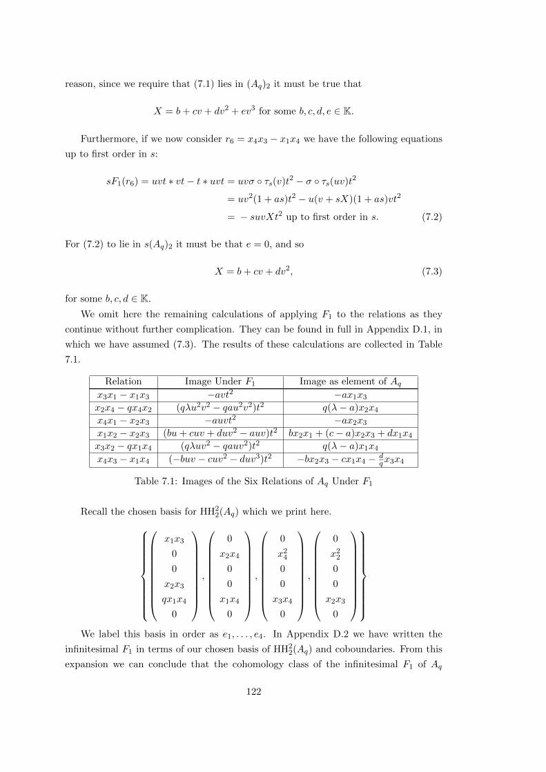
reason, since we require that (7.1) lies in (Aq)2 it must be true that
X = b+ cv + dv2 + ev3 for some b, c, d, e ∈ K.
Furthermore, if we now consider r6 = x4x3 − x1x4 we have the following equations
up to first order in s:
sF1(r6) = uvt ∗ vt− t ∗ uvt = uvσ ◦ τs(v)t2 − σ ◦ τs(uv)t2
= uv2(1 + as)t2 − u(v + sX)(1 + as)vt2
= − suvXt2 up to first order in s. (7.2)
For (7.2) to lie in s(Aq)2 it must be that e = 0, and so
X = b+ cv + dv2, (7.3)
for some b, c, d ∈ K.
We omit here the remaining calculations of applying F1 to the relations as they
continue without further complication. They can be found in full in Appendix D.1, in
which we have assumed (7.3). The results of these calculations are collected in Table
7.1.
Relation Image Under F1 Image as element of Aqx3x1 − x1x3 −avt2 −ax1x3
x2x4 − qx4x2 (qλu2v2 − qau2v2)t2 q(λ− a)x2x4
x4x1 − x2x3 −auvt2 −ax2x3
x1x2 − x2x3 (bu+ cuv + duv2 − auv)t2 bx2x1 + (c− a)x2x3 + dx1x4
x3x2 − qx1x4 (qλuv2 − qauv2)t2 q(λ− a)x1x4
x4x3 − x1x4 (−buv − cuv2 − duv3)t2 −bx2x3 − cx1x4 − dqx3x4
Table 7.1: Images of the Six Relations of Aq Under F1
Recall the chosen basis for HH22(Aq) which we print here.
x1x3
0
0
x2x3
qx1x4
0
,
0
x2x4
0
0
x1x4
0
,
0
x24
0
0
x3x4
0
,
0
x22
0
0
x2x3
0
We label this basis in order as e1, . . . , e4. In Appendix D.2 we have written the
infinitesimal F1 in terms of our chosen basis of HH22(Aq) and coboundaries. From this
expansion we can conclude that the cohomology class of the infinitesimal F1 of Aq
122
associated to the deformation Kq′(u, v)[t, t−1;σ ◦ τs] is
[F1] = a(−e1 − qe2) + (1− q)be4 −(1− q)q
de3 + qλe2. (7.4)
Note that the parameter c does not appear here, since in the expansion in Appendix
D.2 c is a coefficient of a coboundary. This is analogous to behaviour we saw in Lemma
6.4.2 where functions that scaled u had trivial associated infinitesimals.
From Equation (7.4) it is clear that by varying a, b, d and λ we can find a deformation
that corresponds to any chosen direction in HH22(Aq). Thus we have proved:
Theorem 7.3.1. For every isomorphism class of infinitesimal deformations L of Aq
there exists a family of deformations of Qgr(Aq) such that the associated infinitesimal
F1 satisfies:
[F1|Rq ] = L.
7.3.2 Semi-classical Limits as Deformations of A
The preceding calculations have shown that for a general q 6∈ {0, 1} we can find defor-
mations of Qgr(Aq) that correspond to any infinitesimal deformation of Aq. The work
can be split into three steps.
(1) Choose a one-parameter subgroup {τs} ⊆ Aut(Kq(u, v)), with each τs also defin-
ing an automorphism of Kq′(u, v).
(2) Calculate the infinitesimal deformation of Aq associated to the deformation
Kq′(u, v)[t, t−1;σ ◦ τs] of Qgr(Aq)
(3) Find the cohomology class associated to the infinitesimal calculated in Step (2).
Firstly, we note that the subgroup chosen in Section 7.3 also defines a one-parameter
subgroup of Aut(K(u, v)). Secondly, the calculations in Section 7.3 corresponding to
Step (2) were independent of the value of q so long as q 6= 0. Therefore, we can move
to the semi-classical limit q → 1 without changing the validity of the results in the first
two steps.
In Step (3) however, we cannot simply substitute q = 1 into all of the equations
as the cocycles and coboundaries of A and Aq are different. Therefore, we expand the
infinitesimal associated to the deformation in this case in Appendix D.3. We obtain
123

the fact that
[F1] = a
x1x3
0
0
x2x3
x1x4
0
−
0
x2x4
0
0
x1x4
0
+ λ
0
x2x4
0
0
x1x4
0
Therefore we have as kind of ‘semi-classical analogue’ of Theorem 7.3.1:
Proposition 7.3.2. For every isomorphism class of infinitesimal deformations L of A
lying in the space spanned by:
x1x3
0
0
x2x3
x1x4
0
,
0
x2x4
0
0
x1x4
0
there exists a family of deformations of Qgr(A) whose infinitesimal deformation F1
satisfies:
[F1|R ] = L.
Note that these infinitesimals lie in the set Vq (see Section 5.3 for definition), unlike
those discussed in Chapter 6 which lie in Vg. In particular, Aq itself corresponds to
varying λ but having the automorphism be the identity. In this way the family of
deformations Aq of A corresponds to the infinitesimal
0
x2x4
0
0
x1x4
0
∈ HH2
2(A).
124

Chapter 8
A Family of Deformations of A
with the PBW Property
In this chapter we define a new family of algebras that are deformations of the algebra
A. This family gives rise to a 3 dimensional space of infinitesimal deformations that
lie in the unobstructed component of HH22(A) we have called Vq. The main theorem
is Theorem 8.2.1, which states that algebras in this family are PBW. We also classify
elements of this family up to birational equivalence. In particular, in Corollary 8.2.7 we
show that these algebras can have the function skew field Kq(u, v), K(u, v) or D1(K)
depending on the parameters.
The methods used to discover this family are described in Section 8.1. Since the
Hochschild 2-cocycle space is large (22-dimensional), we applied a heuristic search strat-
egy. If the reader prefers they may skip to Section 8.2 for the mathematical content of
the chapter.
8.1 A Heuristic Search Approach to Finding Deforma-
tions
8.1.1 Overview
Our aim is to find families of deformations of A by deforming the set of relations R.
Recall from Definition 1.1.1 that this set is
R =
{r1 := x3x1 − x1x3, r2 := x4x2 − x2x4, r3 := x4x1 − x2x3
r4 := x1x2 − x2x3, r5 := x3x2 − x1x4, r6 := x4x3 − x1x4
}.
Instead of approaching the completely general problem, we will restrict attention to
deformations which satisfy the PBW property with respect to the deformed relations
and the lexicographic ordering given by x2 < x1 < x3 < x4. We call this property P .
125

In order to do this we will use two tools. The first is Bergman’s Diamond Lemma,
which allows us to automate testing a set of relations for the PBW property. The
second is the basis of the Koszul 2-cocycles calculated in Section 3.3, which will reduce
our search space considerably.
Consider the set of PBW reduced monomials in A of degree 2:
Z =
{z1 = x2x2, z2 = x2x1, z3 = x2x3, z4 = x2x4, z5 = x1x1,
z6 = x1x3, z7 = x1x4, z8 = x3x3, z9 = x3x4, z10 = x4x4
}.
We wish to choose elements {∑
i ai,jzi}6j=1 ⊆ spK(Z) so that if we choose deformed
relations by setting for each j ∈ [1, 6]
r′j = rj −∑i
ai,jzi
we obtain an algebra
A′ :=K〈V 〉
({r′1, . . . , r′6})
with property P . One can make small deductions, for example that a8,1 = 0 since
x23 6< x3x1. However, this leaves us with a nearly 60 dimensional problem. We make
some arguments to reduce this.
Each choice of such an ai,j will define a family of algebras. If this is to be a
deformation of A then certainly we expect the vector∑
i ai,1zi...∑
i ai,6zi
to define a Koszul 2-cocycle, since this will be the restriction of the associated infinites-
imal to R. This reduces the search space to a twenty-two dimensional vector space by
Theorem 3.3.1.
Since we wish to study nontrivial deformations, we restrict our attention further to
those elements of this space with nonzero cohomology class. If we label the 22 vectors
of the basis recorded in Appendix A.1.1 as v1, . . . , v22, then in particular the following
are labelled v1, . . . , v8:
126

x1x3
0
0
x2x3
x1x4
0
x23
0
x1x4
0
0
x3x4
x21
0
0
x2x1
x2x3
0
0
x2x4
0
0
x1x4
0
0
x24
0
0
x3x4
0
0
x22
0
0
x2x3
0
0
0
0
x21
0
−x1x3
0
0
0
−x22
0
x2x4
By inspection we can conclude that the coefficients of v2 and v5 must be zero because
in the ordering we have chosen x23 6< x3x1 and x2
4 6< x4x2. For example, if the coefficient
of v2 is b 6= 0 then we have a relation
x3x1 − x1x3 − bx3x3.
But x23 6< x3x1 and so this algebra cannot have property P .
We consider each vi in turn. Since it is not at all clear that by chance the choice of
basis of HH22 we have made is a particularly good one, we make an educated guess as to
a set Ξi of coboundaries that will ‘interact well’ with vi. That is to say that although
v1 itself may not yield an algebra with property P , perhaps if x ∈ Ξ1 then v1 ± x will.
This is a heuristic process; the justification is that it works.
For example, for the vector v1 we choose the following coboundaries as Ξ1 as those
we expect to yield deformations.v10 =
0
0
x2x3
x2x3
−x1x4
−x1x4
, v13 =
0
0
−x2x3
0
x1x4
0
.
We make the assertion that if there is a deformation arising from property P with
associated cohomology class of v1 then it will probably arise using a cocycle of the form
v1 + c1v10 + c2v13 where each ci ∈ {0, 1,−1}. To be clear, this is a heuristic argument,
not a statement of fact.
Once we have found all of the cocycles of this form which define algebras with the
property P we try adding them together. For example, we would try a(v1 + v10) + cv3.
In doing so we can reduce the number of cases to test substantially. We will see that this
process does lead to a new family of algebras corresponding to a choice of infinitesimal
lying in Vq (see Section 5.3).
127
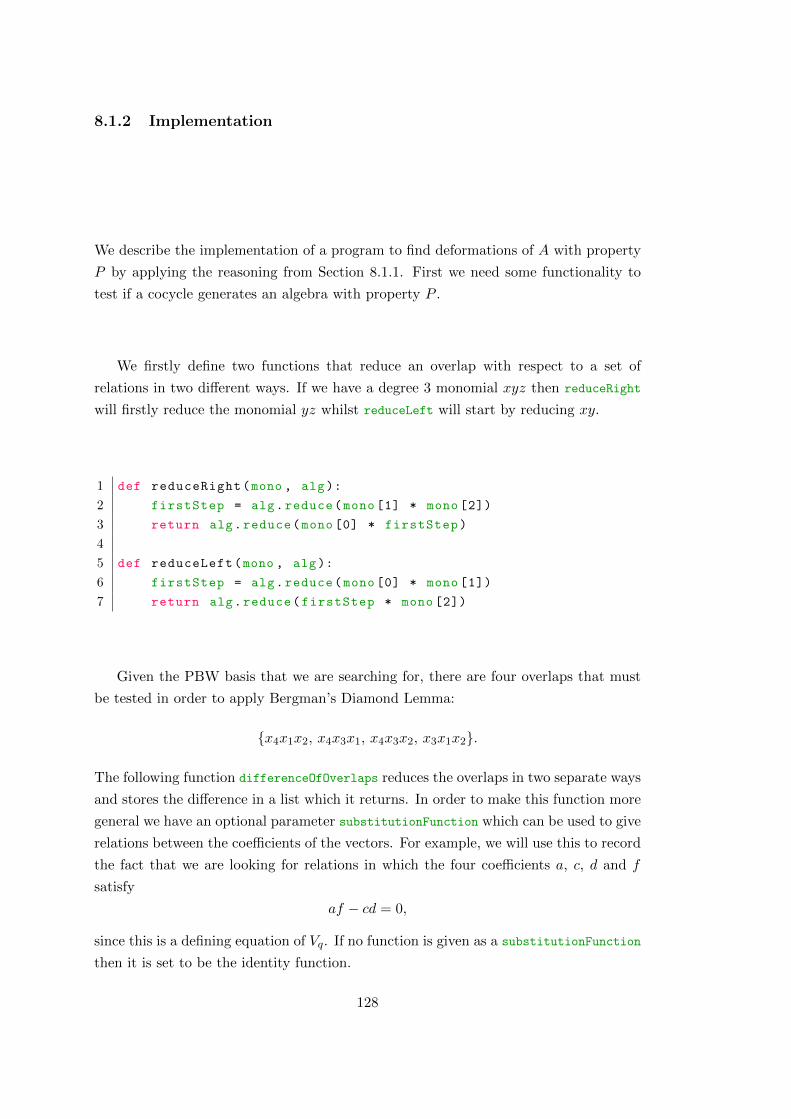
8.1.2 Implementation
We describe the implementation of a program to find deformations of A with property
P by applying the reasoning from Section 8.1.1. First we need some functionality to
test if a cocycle generates an algebra with property P .
We firstly define two functions that reduce an overlap with respect to a set of
relations in two different ways. If we have a degree 3 monomial xyz then reduceRight
will firstly reduce the monomial yz whilst reduceLeft will start by reducing xy.
1 def reduceRight(mono , alg):
2 firstStep = alg.reduce(mono [1] * mono [2])
3 return alg.reduce(mono [0] * firstStep)
4
5 def reduceLeft(mono , alg):
6 firstStep = alg.reduce(mono [0] * mono [1])
7 return alg.reduce(firstStep * mono [2])
Given the PBW basis that we are searching for, there are four overlaps that must
be tested in order to apply Bergman’s Diamond Lemma:
{x4x1x2, x4x3x1, x4x3x2, x3x1x2}.
The following function differenceOfOverlaps reduces the overlaps in two separate ways
and stores the difference in a list which it returns. In order to make this function more
general we have an optional parameter substitutionFunction which can be used to give
relations between the coefficients of the vectors. For example, we will use this to record
the fact that we are looking for relations in which the four coefficients a, c, d and f
satisfy
af − cd = 0,
since this is a defining equation of Vq. If no function is given as a substitutionFunction
then it is set to be the identity function.
128

9 def differenceOfOverlaps(alg , substitutionFunction=None):
10 if substitutionFunction is None:
11 def substitutionFunction(x): return x
12
13 overlaps = [x4 * x1 * x2,
14 x4 * x3 * x1 ,
15 x4 * x3 * x2 ,
16 x3 * x1 * x2]
17 answer = []
18 for overlap in overlaps:
19 right = reduceRight(overlap , alg)
20 left = reduceLeft(overlap , alg)
21 difference =substitutionFunction(right - left)
22 answer.append(difference)
23 return answer
We now give the example of testing for cocycles with nonzero coefficient of v1. To
start we build the list of guesses for cocycles that will lead to deformations with the
property P .
1 guesses = [v1 ,
2 v1 + v10 ,
3 v1 - v10 ,
4 v1 + v13 ,
5 v1 - v13 ,
6 v1 + v10 + v13 ,
7 v1 + v10 - v13 ,
8 v1 - v10 + v13 ,
9 v1 - v10 - v13]
10
11 guesses = [vec * a for vec in guesses]
We now test each of these cocycles in turn and store those that pass the test. The
result of the following script is a list, each element of which corresponds to a family of
deformations of A that is PBW.
129

14 goodCocycles = []
15 for cocycle in guesses:
16 deformedAlgebra = makeAlgebra(cocycle)
17 differences = differenceOfOverlaps(deformedAlgebra)
18 guessWorks = True
19 for difference in differences:
20 if difference != 0:
21 guessWorks = False
22 break
23
24 if guessWorks:
25 goodCocycles.append(cocycle)
The output of this script is the following set:
ax1x3
0
0
ax2x3
ax1x4
0
,
ax1x3
0
ax2x3
ax2x3
0
0
,
ax1x3
0
0
0
ax1x4
ax1x4
.
We have written scripts that do the same as the preceding scripts but for v2, v3 and
v6 which are almost identical. The choices of guesses of Ξi are recorded in Appendix
E.1. Combining these results leads to the following cocycle as defining an algebra with
property P as long as af − cd = 0:
cx21 + ax1x3
fx22 + dx2x4
fx2x1 + dx2x3
0
cx2x3 + ax1x4
cx2x3 + ax1x4
That is to say that the script implies this cocycle will define a PBW algebra with PBW
basis {xi2xj1xk3x
l4}. We verify this fact in Theorem 8.2.1. If one sets a = d and c = f
then this family has an infinitesimal lying in Vg and we obtain algebras which integrate
some of the deformations discussed in Chapter 6. If instead, one sets c = f = 0 then
one recovers the family discussed in Chapter 7. We note that this cocycle is an element
of Vq for any values of a, c, d and f satisfying af − cd = 0.
130
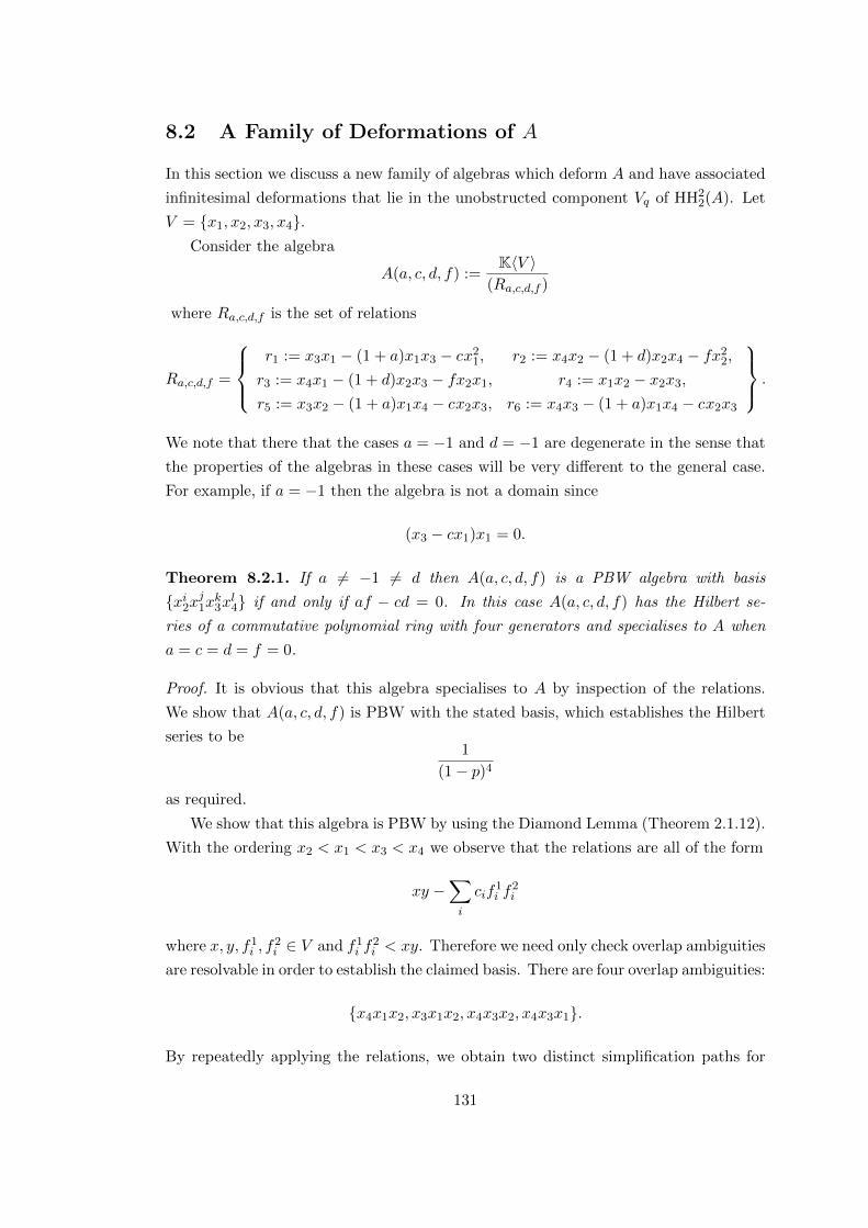
8.2 A Family of Deformations of A
In this section we discuss a new family of algebras which deform A and have associated
infinitesimal deformations that lie in the unobstructed component Vq of HH22(A). Let
V = {x1, x2, x3, x4}.Consider the algebra
A(a, c, d, f) :=K〈V 〉
(Ra,c,d,f )
where Ra,c,d,f is the set of relations
Ra,c,d,f =
r1 := x3x1 − (1 + a)x1x3 − cx2
1, r2 := x4x2 − (1 + d)x2x4 − fx22,
r3 := x4x1 − (1 + d)x2x3 − fx2x1, r4 := x1x2 − x2x3,
r5 := x3x2 − (1 + a)x1x4 − cx2x3, r6 := x4x3 − (1 + a)x1x4 − cx2x3
.
We note that there that the cases a = −1 and d = −1 are degenerate in the sense that
the properties of the algebras in these cases will be very different to the general case.
For example, if a = −1 then the algebra is not a domain since
(x3 − cx1)x1 = 0.
Theorem 8.2.1. If a 6= −1 6= d then A(a, c, d, f) is a PBW algebra with basis
{xi2xj1xk3x
l4} if and only if af − cd = 0. In this case A(a, c, d, f) has the Hilbert se-
ries of a commutative polynomial ring with four generators and specialises to A when
a = c = d = f = 0.
Proof. It is obvious that this algebra specialises to A by inspection of the relations.
We show that A(a, c, d, f) is PBW with the stated basis, which establishes the Hilbert
series to be1
(1− p)4
as required.
We show that this algebra is PBW by using the Diamond Lemma (Theorem 2.1.12).
With the ordering x2 < x1 < x3 < x4 we observe that the relations are all of the form
xy −∑i
cif1i f
2i
where x, y, f1i , f
2i ∈ V and f1
i f2i < xy. Therefore we need only check overlap ambiguities
are resolvable in order to establish the claimed basis. There are four overlap ambiguities:
{x4x1x2, x3x1x2, x4x3x2, x4x3x1}.
By repeatedly applying the relations, we obtain two distinct simplification paths for
131
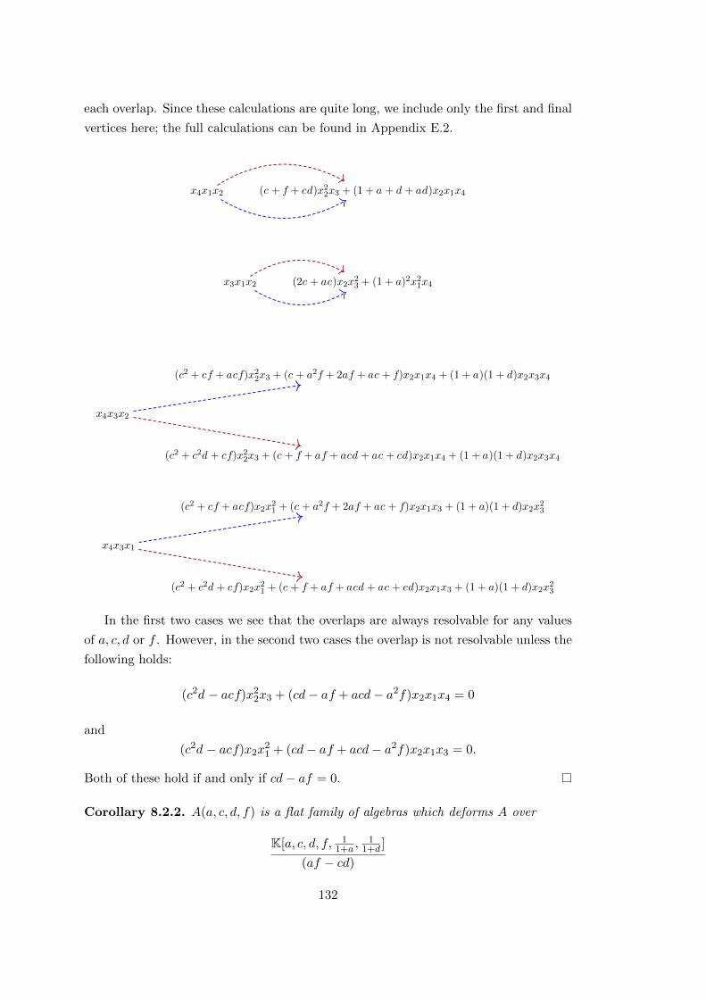
each overlap. Since these calculations are quite long, we include only the first and final
vertices here; the full calculations can be found in Appendix E.2.
x4x1x2 (c + f + cd)x22x3 + (1 + a + d + ad)x2x1x4
x3x1x2 (2c + ac)x2x23 + (1 + a)2x2
1x4
(c2 + cf + acf)x22x3 + (c + a2f + 2af + ac + f)x2x1x4 + (1 + a)(1 + d)x2x3x4
x4x3x2
(c2 + c2d + cf)x22x3 + (c + f + af + acd + ac + cd)x2x1x4 + (1 + a)(1 + d)x2x3x4
(c2 + cf + acf)x2x21 + (c + a2f + 2af + ac + f)x2x1x3 + (1 + a)(1 + d)x2x
23
x4x3x1
(c2 + c2d + cf)x2x21 + (c + f + af + acd + ac + cd)x2x1x3 + (1 + a)(1 + d)x2x
23
In the first two cases we see that the overlaps are always resolvable for any values
of a, c, d or f . However, in the second two cases the overlap is not resolvable unless the
following holds:
(c2d − acf)x22x3 + (cd− af + acd− a2f)x2x1x4 = 0
and
(c2d − acf)x2x21 + (cd− af + acd− a2f)x2x1x3 = 0.
Both of these hold if and only if cd− af = 0.
Corollary 8.2.2. A(a, c, d, f) is a flat family of algebras which deforms A over
K[a, c, d, f, 11+a ,
11+d ]
(af − cd)
132

Proof. This is a standard consequence of the Hilbert series being the same for each
element of the family [Har77, Theorem III.9.9].
Corollary 8.2.3. For any a, c, d, f ∈ K with af − cd = 0 and a 6= −1 6= d, the algebra
A(a, c, d, f) is not noetherian.
Proof. Note that none of the relations of A(a, c, d, f) have x3x4 or x23 appearing with
nonzero coefficient. For this reason we may deduce that for any n ∈ N0 there is no
monomial a ∈ A that has PBW order[a]
satisfy ([a]• xn3x4) 6= 0, except xn3x4 for
itself. We may deduce from this that the equation
n−1∑i=0
xi3x4ai = xn3x4
has no solutions a0, . . . , an−1 ∈ A. Therefore the right ideal generated by {xn3x4}∞n=0 is
not finitely generated.
8.2.1 The Function Skew Field of A(a, c, d, f)
One of the basic properties of a noncommutative projective surface is its function skew
field (see Definition 2.2.8). In this section we find the function skew field of each algebra
in the family of A(a, c, d, f). From here onwards we assume a 6= −1 6= d and af−cd = 0.
Notation 8.2.4. Our convention for Ore extensions is that for a ring R and an auto-
morphism f ∈ Aut(R), then for every r ∈ R we have the following equality in the Ore
extension R[t; f ]:
tr = f(r)t.
Let D be the division ring of the Ore extension K[z][w;α], where α ∈ Aut(K(z)) is
defined by
α(z) =(1 + a)
(1 + d)z − (1 + a)
(1 + d)f + c.
Lemma 8.2.5. The equations
β(z) =z − c1 + a
and β(w) =(z − f)
(1 + d)w
define an automorphism β : D → D.
Proof. It suffices to confirm that β(r) = 0 for r the defining relation of D. By definition
of an Ore extension,
r = wz − α(z)w.
133
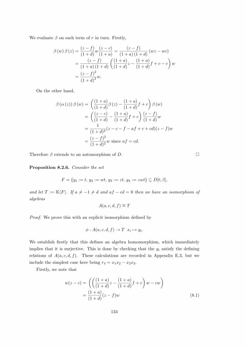
We evaluate β on each term of r in turn. Firstly,
β (w)β (z) =(z − f)
(1 + d)w
(z − c)(1 + a)
=(z − f)
(1 + a) (1 + d)(wz − wc)
=(z − f)
(1 + a) (1 + d)
((1 + a)
(1 + d)z − (1 + a)
(1 + d)f + c− c
)w
=(z − f)2
(1 + d)2w.
On the other hand,
β (α (z))β (w) =
((1 + a)
(1 + d)β (z)− (1 + a)
(1 + d)f + c
)β (w)
=
((z − c)(1 + d)
− (1 + a)
(1 + d)f + c
)(z − f)
(1 + d)w
=1
(1 + d)2(z − c− f − af + c+ cd)(z − f)w
=(z − f)2
(1 + d)2w since af = cd.
Therefore β extends to an automorphism of D.
Proposition 8.2.6. Consider the set
F = {y1 := t, y2 := wt, y3 := zt, y4 := zwt} ⊆ D[t;β],
and let T := K〈F 〉. If a 6= −1 6= d and af − cd = 0 then we have an isomorphism of
algebras
A(a, c, d, f) ∼= T
Proof. We prove this with an explicit isomorphism defined by
φ : A(a, c, d, f)→ T xi 7→ yi.
We establish firstly that this defines an algebra homomorphism, which immediately
implies that it is surjective. This is done by checking that the yi satisfy the defining
relations of A(a, c, d, f). These calculations are recorded in Appendix E.3, but we
include the simplest case here being r4 = x1x2 − x2x3.
Firstly, we note that
w(z − c) =
(((1 + a)
(1 + d)z − (1 + a)
(1 + d)f + c
)w − cw
)=
(1 + a)
(1 + d)(z − f)w (8.1)
134

In particular this implies that
wβ(z) = β(w). (8.2)
Now we can check that whilst
y1y2 = twt = β(w)t2,
we also have that
y2y3 = wtzt = wβ(z)t2 = β(w)t2 by (8.2).
From this calculation, and those contained in Appendix E.3, we may conclude φ
is a surjective algebra homomorphism. Therefore it remains only to verify that φ is
injective. This is done by showing that the Hilbert series of T is the same as that of
A(a, c, d, f). Note that since φ is a surjective (graded) homomorphism, it must be the
case that
dim(A(a, c, d, f)n) ≥ dim(Tn).
We establish that dim(Tn) ≥ dim(An). Since dim(An) = dim(A(a, c, d, f)n by
Theorem 8.2.1, this implies that the Hilbert series of T and A(a, c, d, f) are equal.
Recall that
E = {e1 := t, e2 := ut, e3 := vt, e4 := uvt} ⊆ K(u, v)[t;σ]
generates an algebra isomorphic to A.
We define ∂1 on monomials of A of the form uivjtn by
∂1(uivjtn) = (i, j) ∈ N2.
Then by [RS12, Lemma 4.12 (1)] we know that we have the following equality:
|{∂1(ei1 · · · ein) | i1, . . . , in ∈ [1, 4]}| =(n+ 3
3
)= dim(An).
Likewise, we define ∂2 on polynomials in T of the form g(z)witk, where g(z) ∈ K[z],
by
∂2(g(z)witk) = (i,deg(g)).
We claim for any n ≥ 1 and i1, . . . , in ∈ [1, 4], that
∂1(ei1 · · · ein) = ∂2(yi1 · · · yin).
We prove this by induction on n. The base case of n = 1 is trivial, and so we move to
the inductive step.
Let R = K[z][w;α][t;β]. Then by [BGTV03, Corollary 3.3], R has a basis of the
135

form {ziwjtk}. Furthermore, by [BGTV03, Corollary 2.10 (2)], we have that if X ∈ R∗
and ∂2(X) = (α, β) then if y ∈ F
∂2(Xy) = ∂2(zβwαtky). (8.3)
The following are immediate consequences of the facts that ∂2(α(z)) = (0, 1) =
∂2(β(z)) and ∂2(β(w)) = (1, 1):
∂2(wszr) = (s, r), ∂2(tkzr) = (0, r) and ∂2(tkws) = (s, ks).
Together these imply that for X ∈ T ∗
∂2(zβwαX) = (α, β) + ∂2(X), (8.4)
and that
∂2(tkzc2wc1t) = ∂2(tkzc2) + ∂2(tkwc1) = (c1, c2 + kc1). (8.5)
For the induction then we assume that
(α, β) = ∂1(ei1 · · · eik) = ∂2(yi1 · · · yik)
and that eik+1= uc1vc2t whilst yik+1
= zc2wc1t . On the one hand:
∂1(ei1 · · · eik+1) = ∂1(uαvβtkuc1vc2t)
= ∂1(uα+c1vβ+c2+kc1tk+1) = (α+ c1, β + c2 + kc1).
On the other hand,
∂2(yi1 · · · yik+1) = ∂2(zβwαtkzc2wc1t) by (8.3)
= (α, β) + ∂2(tkzc2wc1t) by (8.4)
= (α, β) + (c1, c2 + kc1) by (8.5)
= ∂1(ei1 · · · eik+1).
This proves the claim. Therefore we have an injection of sets from
{∂1(ei1 · · · ein) | i1, . . . , in ∈ [1, 4]}
into
S := {∂2(yi1 · · · yin) | i1, . . . , in ∈ [1, 4]} .
By definition of Tn, we have that dim(Tn) ≥ |S|, and this injection implies that |S| ≥
136

dim(An). This establishes that
dim(Tn) ≥ dim(An) =
(n+ 3
3
)and so Tn ∼= A(a, c, d, f).
We have as an immediate corollary:
Corollary 8.2.7. The graded quotient ring Qgr(A(a, c, d, f)) is D[t, t−1;β] and D is
the function skew field of A(a, c, d, f).
Proof. This follows since z = y3y−11 and w = y2y
−11 .
This classifies A(a, c, d, f) up to birational equivalence. Furthermore, we obtain:
Corollary 8.2.8. A(a, c, d, f) is a domain.
Proof. Since R = K[z][w;α][t;β] is an iterated Ore extension of a domain, where both
α and β are injective, [GW04, Excercise 2O] implies that R is a domain. Proposition
8.2.6 shows that A(a, c, d, f) is isomorphic to a subalgebra of R and so must also be a
domain.
We further show that, depending on the values of a, c, d and f , the function skew
field D is isomorphic to the division ring of one of three algebras: the polynomial ring
K[u, v], the quantum plane Kq[u, v] or the Weyl algebra
A1(K) =K〈u, v〉
(vu− uv + 1).
The division ring of A1(K) is written D1(K).
Proposition 8.2.9. D is isomorphic to
(a) K(u, v) if a = d and c = f .
(b) D1(K) if a = d = 0 and c 6= f .
(c) Kq(u, v) where q = (1+d)(1+a) if a 6= d.
Proof. (a) This follows immediately from the definition of α since if a = d and c = f
then α(z) = z.
(b) Let u = zwf−c and v = w−1. Note that since α(z) = z − (f − c) we have
w
(z
f − c
)=
(z
f − c− 1
)w.
137
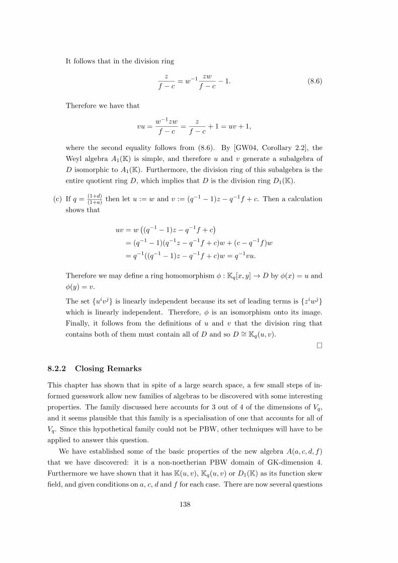
It follows that in the division ring
z
f − c= w−1 zw
f − c− 1. (8.6)
Therefore we have that
vu =w−1zw
f − c=
z
f − c+ 1 = uv + 1,
where the second equality follows from (8.6). By [GW04, Corollary 2.2], the
Weyl algebra A1(K) is simple, and therefore u and v generate a subalgebra of
D isomorphic to A1(K). Furthermore, the division ring of this subalgebra is the
entire quotient ring D, which implies that D is the division ring D1(K).
(c) If q = (1+d)(1+a) then let u := w and v := (q−1 − 1)z − q−1f + c. Then a calculation
shows that
uv = w((q−1 − 1)z − q−1f + c
)= (q−1 − 1)(q−1z − q−1f + c)w + (c− q−1f)w
= q−1((q−1 − 1)z − q−1f + c)w = q−1vu.
Therefore we may define a ring homomorphism φ : Kq[x, y]→ D by φ(x) = u and
φ(y) = v.
The set {uivj} is linearly independent because its set of leading terms is {ziwj}which is linearly independent. Therefore, φ is an isomorphism onto its image.
Finally, it follows from the definitions of u and v that the division ring that
contains both of them must contain all of D and so D ∼= Kq(u, v).
8.2.2 Closing Remarks
This chapter has shown that in spite of a large search space, a few small steps of in-
formed guesswork allow new families of algebras to be discovered with some interesting
properties. The family discussed here accounts for 3 out of 4 of the dimensions of Vq,
and it seems plausible that this family is a specialisation of one that accounts for all of
Vq. Since this hypothetical family could not be PBW, other techniques will have to be
applied to answer this question.
We have established some of the basic properties of the new algebra A(a, c, d, f)
that we have discovered: it is a non-noetherian PBW domain of GK-dimension 4.
Furthermore we have shown that it has K(u, v), Kq(u, v) or D1(K) as its function skew
field, and given conditions on a, c, d and f for each case. There are now several questions
138

which would be very interesting for further investigation. The most interesting of these
are whether A(a, c, d, f) is ever AS-Gorenstein, since none of the previously studied
deformations of A have this property. It would also be fascinating if there are families
of deformations of A that specialise to A(a, c, d, f) for which the generic element has
the noetherian property.
139

140

Appendices
141


Appendix A
Bases Relevant to Calculations
on Hochschild Cohomology
Recall that both A and Aq are PBW algebras with respect to the lexicographic ordering
on monomials induced by the ordering of generators
x2 < x1 < x3 < x4.
With this in mind we choose a basis for Kn in degree m. We start by taking monomials
of degree m in order
m1 := xm2 < m2 := xm−12 x1 < m3 . . . < mz := xm4
where z =(m+3
3
). Then the if Kn is k dimensional the basis is the following ordered
set of vectors with k components (using notation as in Notation 3.2.1).
m1
0...
0
,
m2
0...
0
, . . . ,
mz
0...
0
,
0
m1
...
0
, . . . ,
0
0...
mz
A.1 Calculations For A
A.1.1 Basis of the Kernel of k3
The content of this section is calculated using the ‘Sage’ script discussed in Section 3.3,
being a basis for the space Ker(k3). This space is 22 dimensional and is written using
the vector notation defined in Notation 3.2.1. We have reordered the output so that
the first eight vectors have cohomology classes that are a basis of the cohomology space
(compare the following with the basis presented in Section A.1.2).
143
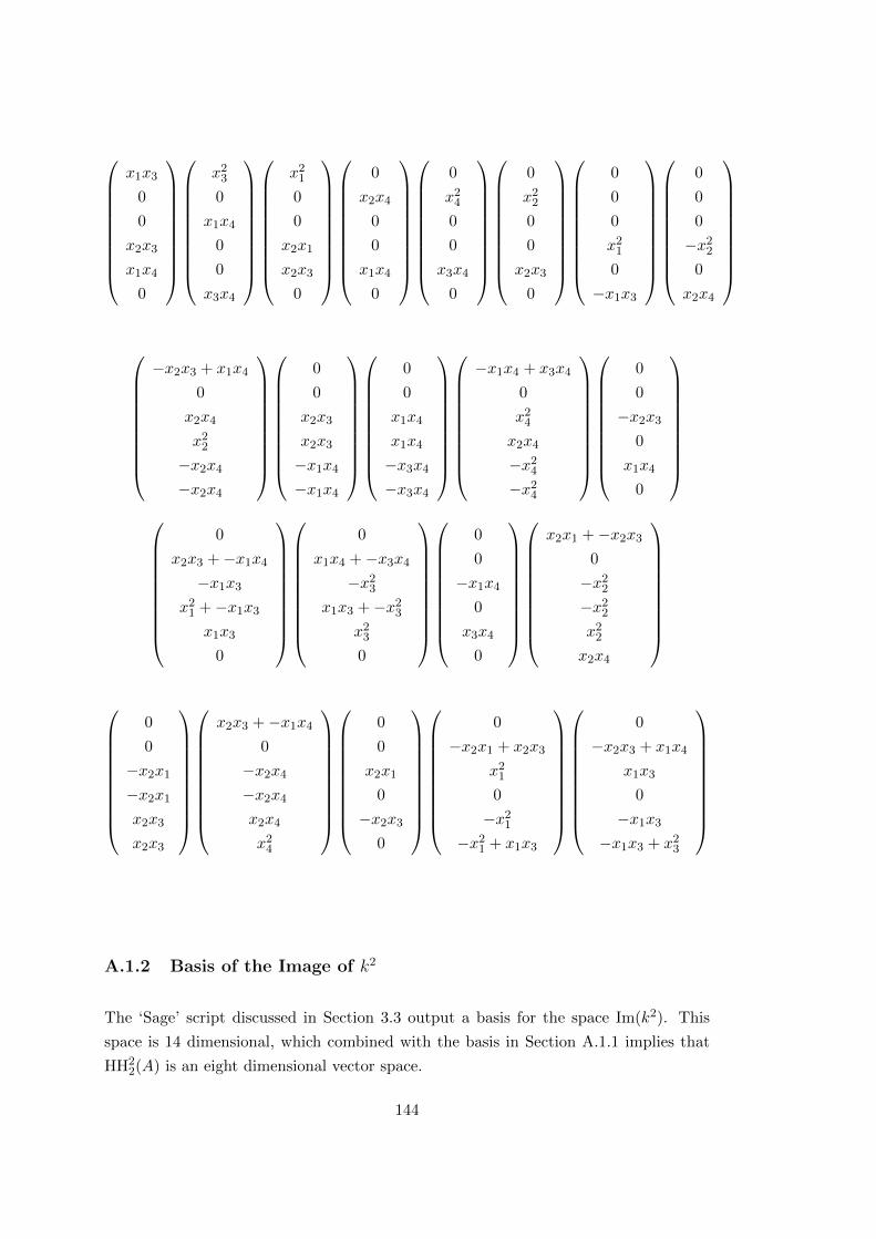
x1x3
0
0
x2x3
x1x4
0
x23
0
x1x4
0
0
x3x4
x21
0
0
x2x1
x2x3
0
0
x2x4
0
0
x1x4
0
0
x24
0
0
x3x4
0
0
x22
0
0
x2x3
0
0
0
0
x21
0
−x1x3
0
0
0
−x22
0
x2x4
−x2x3 + x1x4
0
x2x4
x22
−x2x4
−x2x4
0
0
x2x3
x2x3
−x1x4
−x1x4
0
0
x1x4
x1x4
−x3x4
−x3x4
−x1x4 + x3x4
0
x24
x2x4
−x24
−x24
0
0
−x2x3
0
x1x4
0
0
x2x3 +−x1x4
−x1x3
x21 +−x1x3
x1x3
0
0
x1x4 +−x3x4
−x23
x1x3 +−x23
x23
0
0
0
−x1x4
0
x3x4
0
x2x1 +−x2x3
0
−x22
−x22
x22
x2x4
0
0
−x2x1
−x2x1
x2x3
x2x3
x2x3 +−x1x4
0
−x2x4
−x2x4
x2x4
x24
0
0
x2x1
0
−x2x3
0
0
−x2x1 + x2x3
x21
0
−x21
−x21 + x1x3
0
−x2x3 + x1x4
x1x3
0
−x1x3
−x1x3 + x23
A.1.2 Basis of the Image of k2
The ‘Sage’ script discussed in Section 3.3 output a basis for the space Im(k2). This
space is 14 dimensional, which combined with the basis in Section A.1.1 implies that
HH22(A) is an eight dimensional vector space.
144
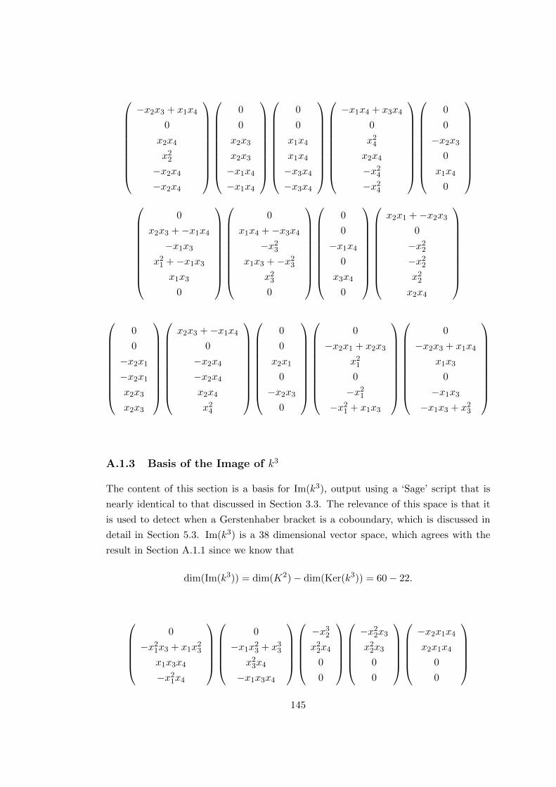
−x2x3 + x1x4
0
x2x4
x22
−x2x4
−x2x4
0
0
x2x3
x2x3
−x1x4
−x1x4
0
0
x1x4
x1x4
−x3x4
−x3x4
−x1x4 + x3x4
0
x24
x2x4
−x24
−x24
0
0
−x2x3
0
x1x4
0
0
x2x3 +−x1x4
−x1x3
x21 +−x1x3
x1x3
0
0
x1x4 +−x3x4
−x23
x1x3 +−x23
x23
0
0
0
−x1x4
0
x3x4
0
x2x1 +−x2x3
0
−x22
−x22
x22
x2x4
0
0
−x2x1
−x2x1
x2x3
x2x3
x2x3 +−x1x4
0
−x2x4
−x2x4
x2x4
x24
0
0
x2x1
0
−x2x3
0
0
−x2x1 + x2x3
x21
0
−x21
−x21 + x1x3
0
−x2x3 + x1x4
x1x3
0
−x1x3
−x1x3 + x23
A.1.3 Basis of the Image of k3
The content of this section is a basis for Im(k3), output using a ‘Sage’ script that is
nearly identical to that discussed in Section 3.3. The relevance of this space is that it
is used to detect when a Gerstenhaber bracket is a coboundary, which is discussed in
detail in Section 5.3. Im(k3) is a 38 dimensional vector space, which agrees with the
result in Section A.1.1 since we know that
dim(Im(k3)) = dim(K2)− dim(Ker(k3)) = 60− 22.
0
−x21x3 + x1x
23
x1x3x4
−x21x4
0
−x1x23 + x3
3
x23x4
−x1x3x4
−x3
2
x22x4
0
0
−x2
2x3
x22x3
0
0
−x2x1x4
x2x1x4
0
0
145

−x2
2x4
x2x24
0
0
−x2x
23
x2x1x3
0
0
−x2
1x4
x2x23
0
0
−x2x3x4
x2x3x4
0
0
−x1x3x4
x21x4
0
0
−x1x
24
x1x24
0
0
−x2x
24
x34
0
0
0
0
−x2x1x4
x22x3
0
0
−x2x1x3
x2x1x3
0
0
−x2x23
x2x23
0
0
−x2x3x4
x2x1x4
0
0
−x31
x21x3
0
0
−x21x4
x21x4
0
0
−x1x23
x33
0
0
−x1x3x4
x1x3x4
0
0
−x1x24
x2x3x4
0
x2x3x4 +−x1x24
x34
−x2x24
0
0
−x21x3
x1x23
0
x2x1x4 +−x2x3x4
x2x24
−x22x4
0
−x31 + x2
1x3
x21x4
−x2x23
0
0
x3x24
−x1x24
0
0
x22x3
−x22x1
x2x3x4
−x22x3
−x22x4
x22x4
x1x24
−x2x1x4
−x2x24
x2x24
x21x3
−x21x3
−x21x4
x2x1x3
x1x23
−x1x23
−x1x3x4
x2x23
x33
−x33
−x23x4
x21x4
x23x4
−x1x3x4
−x3x24
x1x24
x3x
24
−x2x3x4
−x34
x34
−x3
1 + x21x3
0
x2x1x3
−x2x21
x2x1x4
−x22x1
−x32
x32
x2x1x3
−x2x21
−x22x3
x22x1
0
x22x3 +−x2x1x4
x22x4
−x32
146

A.1.4 Gerstenhaber Brackets of the Basis of HH22(A)
The content of this section is the set of vectors [bi, bj ] calculated in the script discussed
in Section 5.3. Note the vectors lie in K3(A).
[b1, b1] =
0
0
0
0
, [b1, b2] =
0
0
0
0
, [b1, b3] =
x2x
23
−x2x1x3
0
0
, [b1, b4] =
0
0
x2x3x4
−x2x1x4
,
[b1, b5] =
−x1x3x4
0
0
−x2x3x4
, [b1, b6] =
x2x
23
0
2x2x1x4
−x22x3
, [b1, b7] =
0
−x21x3
−x21x4
0
,
[b1, b8] =
−x2x3x4
0
0
−x22x4
, [b2, b2] =
2x2
3x4
−2x1x3x4
0
0
, [b2, b3] =
x2
1x4
−x2x23
0
0
,
[b2, b4] =
0
x21x4
x1x24
0
, [b2, b5] =
−x2
3x4
x1x3x4
x3x24
−x1x24
, [b2, b6] =
x2
1x4
x2x23
x2x3x4
x2x1x4
,
[b2, b7] =
−2x1x
23
x21x3
0
−2x2x23 + x2
1x4
, [b2, b8] =
0
−x2x3x4
0
−x22x4
, [b3, b3] =
2x2x1x3
−2x2x21
0
0
,
[b3, b4] =
−x2x
23
0
0
−x22x3
, [b3, b5] =
−2x2
1x4
0
−x2x3x4
−x2x1x4
, [b3, b6] =
0
0
x22x3
−x22x1
,
[b3, b7] =
−x3
1 + x21x3
−x31
−x2x23 + x2x1x3
−x2x21
, [b3, b8] =
−x2
2x3
0
−x22x4
0
, [b4, b4] =
0
0
0
0
,
147
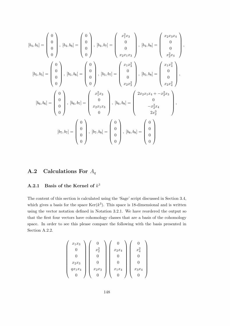
[b4, b5] =
0
0
0
0
, [b4, b6] =
0
0
0
0
, [b4, b7] =
x2
1x3
0
0
x2x1x3
, [b4, b8] =
x2x3x4
0
0
x22x4
,
[b5, b5] =
0
0
0
0
, [b5, b6] =
0
0
0
0
, [b5, b7] =
x1x
23
0
0
x2x23
, [b5, b8] =
x1x
24
0
0
x2x24
,
[b6, b6] =
0
0
0
0
, [b6, b7] =
x2
1x3
0
x2x1x3
0
, [b6, b8] =
2x2x1x4 +−x2
2x3
0
−x22x4
2x32
,
[b7, b7] =
0
0
0
0
, [b7, b8] =
0
0
0
0
, [b8, b8] =
0
0
0
0
A.2 Calculations For Aq
A.2.1 Basis of the Kernel of k3
The content of this section is calculated using the ‘Sage’ script discussed in Section 3.4,
which gives a basis for the space Ker(k3). This space is 18-dimensional and is written
using the vector notation defined in Notation 3.2.1. We have reordered the output so
that the first four vectors have cohomology classes that are a basis of the cohomology
space. In order to see this please compare the following with the basis presented in
Section A.2.2.
x1x3
0
0
x2x3
qx1x4
0
0
x22
0
0
x2x3
0
0
x2x4
0
0
x1x4
0
0
x24
0
0
x3x4
0
148

−x2x3 + qx1x4
0
qx2x4
x22
−qx2x4
−x2x4
0
−qx2x3 + qx1x4
x1x3
0
−qx1x3
−x1x3 + x23
0
x2x3 − qx1x4
−x1x3
x21 − x1x3
x1x3
0
0
x2x3 − qx2x1
x21
0
−qx21
−x21 + x1x3
0
x1x4 − qx3x4
−x23
x1x3 − x23
x23
0
0
(1− q)x24
−x1x4
0
x3x4
0
0
0
x1x4
qx1x4
−qx3x4
−x3x4
0
(1− q)x22
x2x1
0
−qx2x3
0
0
0
−x2x1
−x2x1
x2x3
x2x3
x2x3 − x1x4
0
−x2x4
−x2x4
qx2x4
x24
x2x1 − x2x3
0
−x2d
−x22
x2d
qx2x4
0
0
x2x3
0
−qx1x4
0
0
0
x2x3
x2x3
−qx1x4
−x1x4
x3x4 − x1x4
0
x24
qx2x4
−qx24
−x24
A.2.2 Basis of the Image of k2
We include the output of the ‘Sage’ script discussed in Section 3.4, being a basis for the
space Im(k2). This space is 14 dimensional, which combined with the basis in Section
A.2.1 implies that HH22(Aq) is an four dimensional vector space.
−x2x3 + qx1x4
0
qx2x4
x22
−qx2x4
−x2x4
0
−qx2x3 + qx1x4
x1x3
0
−qx1x3
−x1x3 + x23
0
x2x3 − qx1x4
−x1x3
x21 − x1x3
x1x3
0
149

0
x2x3 − qx2x1
x21
0
−qx21
−x21 + x1x3
0
x1x4 − qx3x4
−x23
x1x3 − x23
x23
0
0
(1− q)x24
−x1x4
0
x3x4
0
0
0
x1x4
qx1x4
−qx3x4
−x3x4
0
(1− q)x22
x2x1
0
−qx2x3
0
0
0
−x2x1
−x2x1
x2x3
x2x3
x2x3 − x1x4
0
−x2x4
−x2x4
qx2x4
x24
x2x1 − x2x3
0
−x2d
−x22
x2d
qx2x4
0
0
x2x3
0
−qx1x4
0
0
0
x2x3
x2x3
−qx1x4
−x1x4
x3x4 − x1x4
0
x24
qx2x4
−qx24
−x24
A.2.3 Basis of the Image of k3
The content of this section is a basis for Im(k3), output using a ‘Sage’ script that is
nearly identical to that discussed in Section 3.4. The relevance of this space is that it
is used to detect when a Gerstenhaber bracket is a coboundary, which is discussed in
detail in Section 5.4. Im(k3) is a 42 dimensional vector space, which agrees with the
result in Section A.2.1 since we know that
dim(Im(k3)) = dim(K2)− dim(Ker(k3)) = 60− 18.
x3
2
−q2x22x4
0
0
x22x3
0
q2x22x4
0
x22x4
−x2x24
0
0
q2x2x1x3
−qx2x21
0
(−1 + q2)x22x1
qx2x1x4
0
0
x32
150
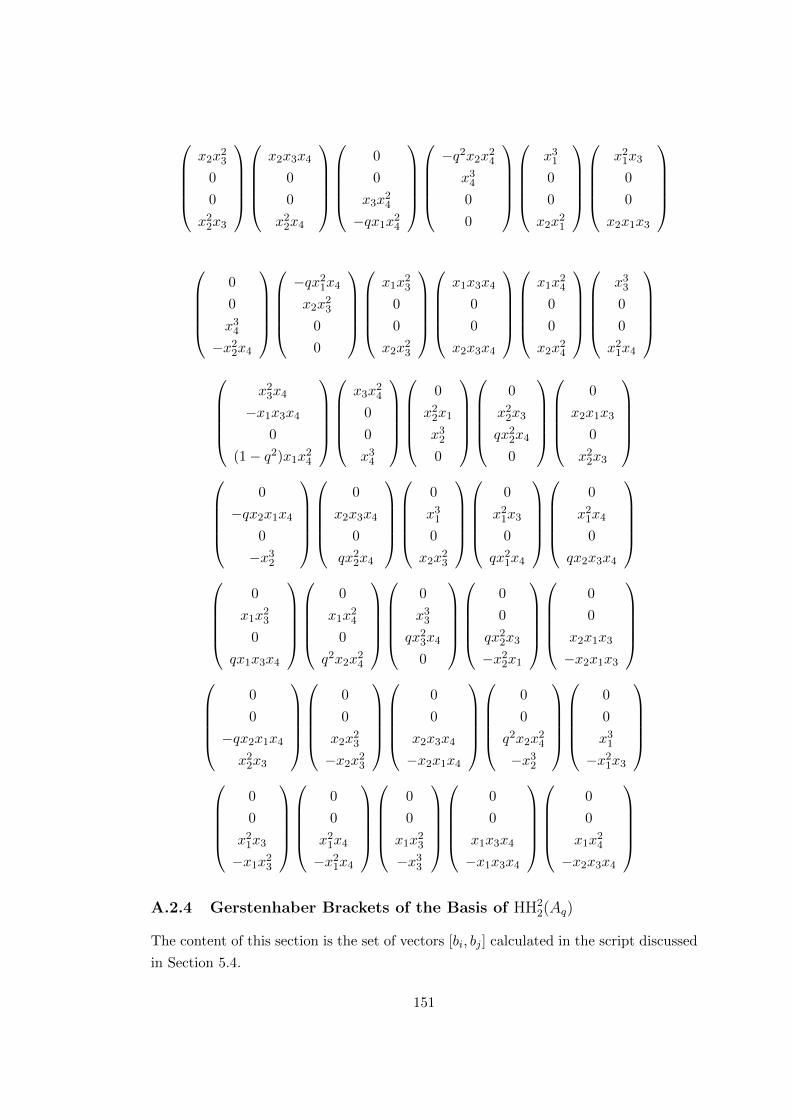
x2x
23
0
0
x22x3
x2x3x4
0
0
x22x4
0
0
x3x24
−qx1x24
−q2x2x
24
x34
0
0
x31
0
0
x2x21
x21x3
0
0
x2x1x3
0
0
x34
−x22x4
−qx2
1x4
x2x23
0
0
x1x23
0
0
x2x23
x1x3x4
0
0
x2x3x4
x1x24
0
0
x2x24
x33
0
0
x21x4
x23x4
−x1x3x4
0
(1− q2)x1x24
x3x24
0
0
x34
0
x22x1
x32
0
0
x22x3
qx22x4
0
0
x2x1x3
0
x22x3
0
−qx2x1x4
0
−x32
0
x2x3x4
0
qx22x4
0
x31
0
x2x23
0
x21x3
0
qx21x4
0
x21x4
0
qx2x3x4
0
x1x23
0
qx1x3x4
0
x1x24
0
q2x2x24
0
x33
qx23x4
0
0
0
qx22x3
−x22x1
0
0
x2x1x3
−x2x1x3
0
0
−qx2x1x4
x22x3
0
0
x2x23
−x2x23
0
0
x2x3x4
−x2x1x4
0
0
q2x2x24
−x32
0
0
x31
−x21x3
0
0
x21x3
−x1x23
0
0
x21x4
−x21x4
0
0
x1x23
−x33
0
0
x1x3x4
−x1x3x4
0
0
x1x24
−x2x3x4
A.2.4 Gerstenhaber Brackets of the Basis of HH2
2(Aq)
The content of this section is the set of vectors [bi, bj ] calculated in the script discussed
in Section 5.4.
151

[b1, b1] =
0
0
0
0
, [b1, b2] =
0
0
x2x3x4
−x2x1x4
, [b1, b3] =
−x1x3x4
0
0
−x2x3x4
,
[b1, b4] =
x2x
23
0
2qx2x1x4
−x22x3
, [b2, b2] =
0
0
0
0
, [b2, b3] =
0
0
0
0
,
[b2, b4] =
0
0
0
0
, [b3, b3] =
0
0
0
0
, [b3, b4] =
0
0
0
0
, [b4, b4] =
0
0
0
0
,
152

Appendix B
Polygnome Source Code
In this appendix we gather together relevant pieces of source code from ‘Polygnome’
and explain any particularly opaque segments. Polygnome is a Python software package
written by the author and freely available online [Cam]. The package was designed for
manipulating elements of PBW algebras and was specifically tailored to allow the map
m2 to be defined in it. After a review of the software at the time, none was found that
would the allow low level interaction with reduction sequences that was required for
this task.
Note that in this code a ‘Decorator’ called bimoduleMapDecorator is used. A decora-
tor in Python modifies a function so that the same code does not have to be rewritten
multiple times. In this case, the decorator takes a function defined on a generating set
for a free bimodule over an algebra and modifies it to be defined on the whole bimodule.
Note that the decorator takes as arguments the domain and codomain of the bimodule
map.
B.1 Koszul Boundary Maps
The following code defines the boundary maps k_1 and k_3. It also defines the dual
map k_3Dual. For a in depth discussion of the following code and the definition of k_2
please see Section 3.2.1.
153
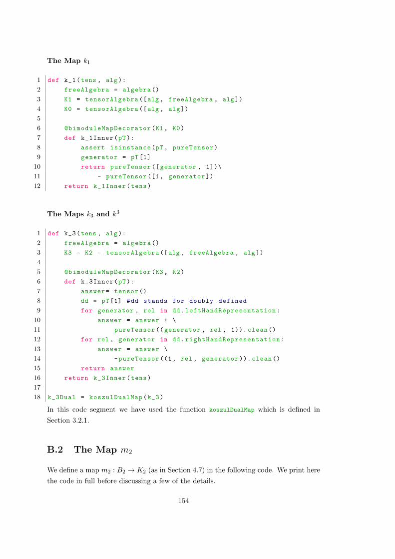
The Map k1
1 def k_1(tens , alg):
2 freeAlgebra = algebra ()
3 K1 = tensorAlgebra ([alg , freeAlgebra , alg])
4 K0 = tensorAlgebra ([alg , alg])
5
6 @bimoduleMapDecorator(K1, K0)
7 def k_1Inner(pT):
8 assert isinstance(pT , pureTensor)
9 generator = pT[1]
10 return pureTensor ([generator , 1])\
11 - pureTensor ([1, generator ])
12 return k_1Inner(tens)
The Maps k3 and k3
1 def k_3(tens , alg):
2 freeAlgebra = algebra ()
3 K3 = K2 = tensorAlgebra ([alg , freeAlgebra , alg])
4
5 @bimoduleMapDecorator(K3, K2)
6 def k_3Inner(pT):
7 answer= tensor ()
8 dd = pT[1] #dd stands for doubly defined
9 for generator , rel in dd.leftHandRepresentation:
10 answer = answer + \
11 pureTensor ((generator , rel , 1)). clean ()
12 for rel , generator in dd.rightHandRepresentation:
13 answer = answer \
14 -pureTensor ((1, rel , generator )). clean()
15 return answer
16 return k_3Inner(tens)
17
18 k_3Dual = koszulDualMap(k_3)
In this code segment we have used the function koszulDualMap which is defined in
Section 3.2.1.
B.2 The Map m2
We define a map m2 : B2 → K2 (as in Section 4.7) in the following code. We print here
the code in full before discussing a few of the details.
154
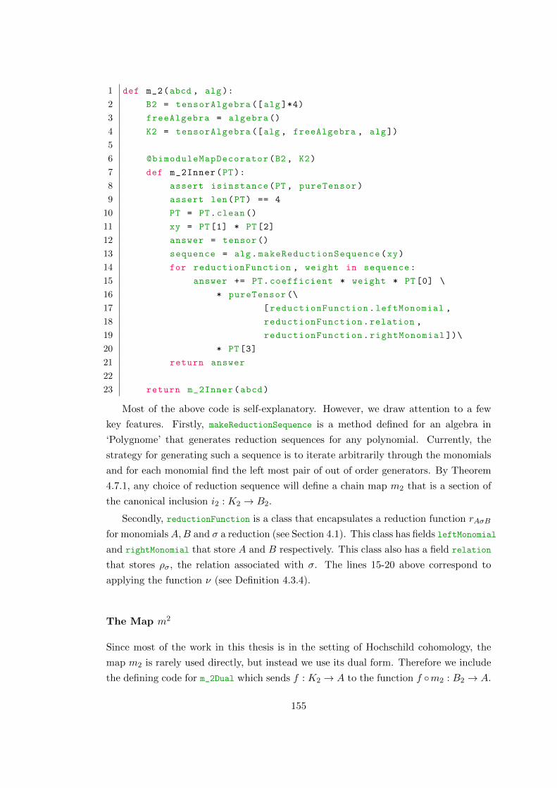
1 def m_2(abcd , alg):
2 B2 = tensorAlgebra ([alg ]*4)
3 freeAlgebra = algebra ()
4 K2 = tensorAlgebra ([alg , freeAlgebra , alg])
5
6 @bimoduleMapDecorator(B2, K2)
7 def m_2Inner(PT):
8 assert isinstance(PT, pureTensor)
9 assert len(PT) == 4
10 PT = PT.clean()
11 xy = PT[1] * PT[2]
12 answer = tensor ()
13 sequence = alg.makeReductionSequence(xy)
14 for reductionFunction , weight in sequence:
15 answer += PT.coefficient * weight * PT[0] \
16 * pureTensor (\
17 [reductionFunction.leftMonomial ,
18 reductionFunction.relation ,
19 reductionFunction.rightMonomial ])\
20 * PT[3]
21 return answer
22
23 return m_2Inner(abcd)
Most of the above code is self-explanatory. However, we draw attention to a few
key features. Firstly, makeReductionSequence is a method defined for an algebra in
‘Polygnome’ that generates reduction sequences for any polynomial. Currently, the
strategy for generating such a sequence is to iterate arbitrarily through the monomials
and for each monomial find the left most pair of out of order generators. By Theorem
4.7.1, any choice of reduction sequence will define a chain map m2 that is a section of
the canonical inclusion i2 : K2 → B2.
Secondly, reductionFunction is a class that encapsulates a reduction function rAσB
for monomialsA,B and σ a reduction (see Section 4.1). This class has fields leftMonomial
and rightMonomial that store A and B respectively. This class also has a field relation
that stores ρσ, the relation associated with σ. The lines 15-20 above correspond to
applying the function ν (see Definition 4.3.4).
The Map m2
Since most of the work in this thesis is in the setting of Hochschild cohomology, the
map m2 is rarely used directly, but instead we use its dual form. Therefore we include
the defining code for m_2Dual which sends f : K2 → A to the function f ◦m2 : B2 → A.
155

1 def m_2Dual(func):
2 def newFunc(tensor ):
3 return func(m_2(tensor , func.algebra ))
4 return newFunc
B.3 The Map i∗
The following code defines the injection in : Kn → Bn in the cases n = 2 and n = 3.
The dual map i3 is also defined below.
The Map i2
1 def i_2(tens , alg):
2 freeAlgebra = algebra ()
3 B2 = tensorAlgebra ([alg] * 4)
4 K2 = tensorAlgebra ([alg , freeAlgebra , alg])
5
6 @bimoduleMapDecorator(K2, B2)
7 def i_2Inner(pT):
8 answer = tensor ()
9 rel = pT[1]
10 for term in rel.leadingMonomial:
11 answer = answer \
12 + term.coefficient \
13 * pureTensor ((1, term[0], term[1], 1))
14 for term in rel.lowerOrderTerms:
15 answer = answer \
16 - term.coefficient \
17 * pureTensor ((1, term[0], term[1], 1))
18 return answer
19 return i_2Inner(tens)
156
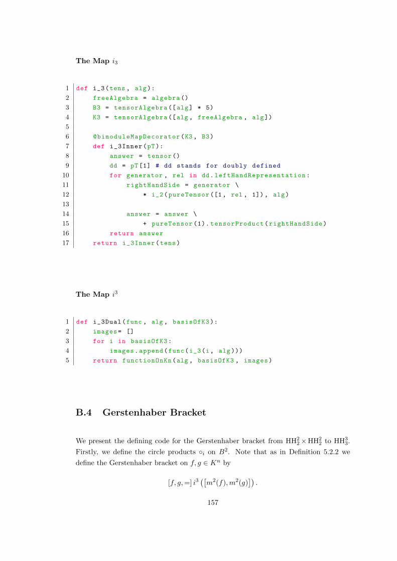
The Map i3
1 def i_3(tens , alg):
2 freeAlgebra = algebra ()
3 B3 = tensorAlgebra ([alg] * 5)
4 K3 = tensorAlgebra ([alg , freeAlgebra , alg])
5
6 @bimoduleMapDecorator(K3, B3)
7 def i_3Inner(pT):
8 answer = tensor ()
9 dd = pT[1] # dd stands for doubly defined
10 for generator , rel in dd.leftHandRepresentation:
11 rightHandSide = generator \
12 * i_2(pureTensor ([1, rel , 1]), alg)
13
14 answer = answer \
15 + pureTensor (1). tensorProduct(rightHandSide)
16 return answer
17 return i_3Inner(tens)
The Map i3
1 def i_3Dual(func , alg , basisOfK3 ):
2 images= []
3 for i in basisOfK3:
4 images.append(func(i_3(i, alg )))
5 return functionOnKn(alg , basisOfK3 , images)
B.4 Gerstenhaber Bracket
We present the defining code for the Gerstenhaber bracket from HH22×HH2
2 to HH33.
Firstly, we define the circle products ◦i on B2. Note that as in Definition 5.2.2 we
define the Gerstenhaber bracket on f, g ∈ Kn by
[f, g,=] i3([m2(f),m2(g)
]).
157
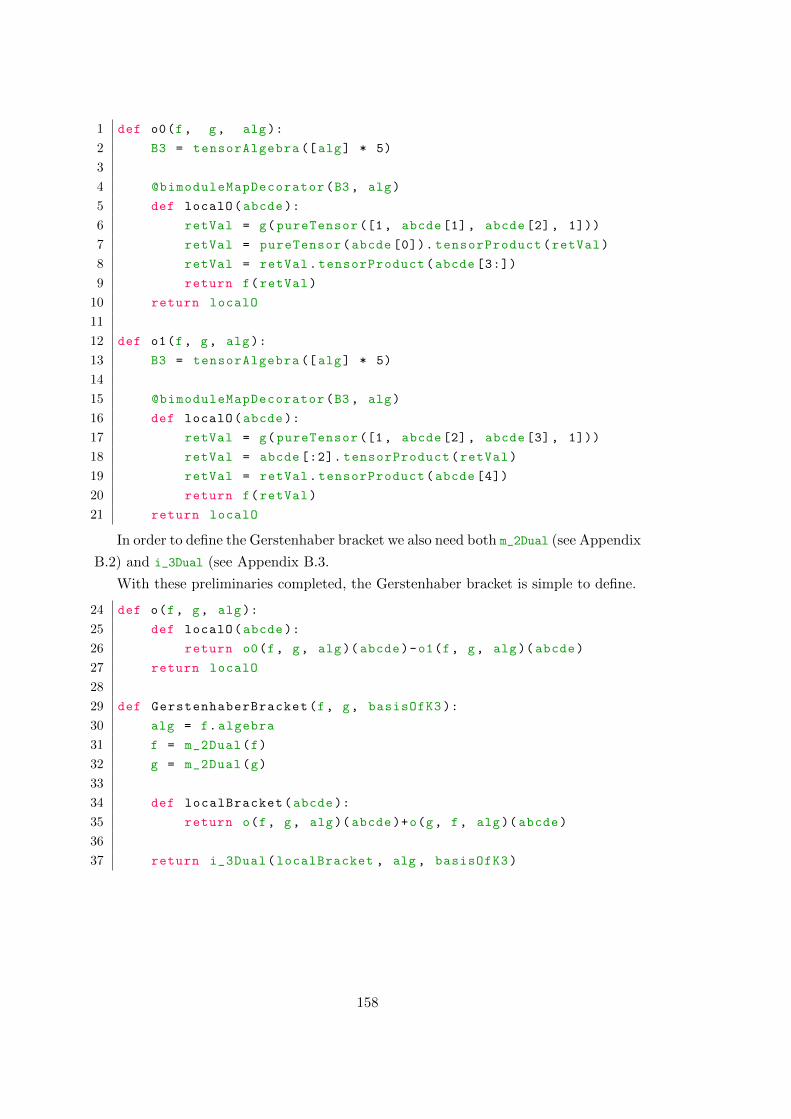
1 def o0(f, g, alg):
2 B3 = tensorAlgebra ([alg] * 5)
3
4 @bimoduleMapDecorator(B3, alg)
5 def localO(abcde):
6 retVal = g(pureTensor ([1, abcde[1], abcde[2], 1]))
7 retVal = pureTensor(abcde [0]). tensorProduct(retVal)
8 retVal = retVal.tensorProduct(abcde [3:])
9 return f(retVal)
10 return localO
11
12 def o1(f, g, alg):
13 B3 = tensorAlgebra ([alg] * 5)
14
15 @bimoduleMapDecorator(B3, alg)
16 def localO(abcde):
17 retVal = g(pureTensor ([1, abcde[2], abcde[3], 1]))
18 retVal = abcde [:2]. tensorProduct(retVal)
19 retVal = retVal.tensorProduct(abcde [4])
20 return f(retVal)
21 return localO
In order to define the Gerstenhaber bracket we also need both m_2Dual (see Appendix
B.2) and i_3Dual (see Appendix B.3.
With these preliminaries completed, the Gerstenhaber bracket is simple to define.
24 def o(f, g, alg):
25 def localO(abcde):
26 return o0(f, g, alg)( abcde)-o1(f, g, alg)( abcde)
27 return localO
28
29 def GerstenhaberBracket(f, g, basisOfK3 ):
30 alg = f.algebra
31 f = m_2Dual(f)
32 g = m_2Dual(g)
33
34 def localBracket(abcde):
35 return o(f, g, alg)( abcde)+o(g, f, alg)( abcde)
36
37 return i_3Dual(localBracket , alg , basisOfK3)
158

Appendix C
Calculations Relevant to
Deformations of A Arising from
Geometric Automorphisms of
K(u, v)
C.1 Calculation of F1 Applied to the Relations of A
We include here the full derivations of F1(r) for each relation of the algebra A. These
are recorded in Section 6.3 in Table 6.1. Recall that in the following calculations U(s)
and V (s) satisfy:
U(0) = uv and V (0) = v.
1.
F1(r1) =∂(F (r1))
∂s
∣∣∣∣s=0
=∂(F (x3x1 − x1x3))
∂s
∣∣∣∣s=0
=∂(vt2 − tvt)
∂s
∣∣∣∣s=0
=∂(vt2 − V (s)t2)
∂s
∣∣∣∣s=0
= −∂(V (s)t2)
∂s
∣∣∣∣s=0
= −V ′(0)t2
159

2.
F1(r2) =∂(F (x4x2 − x2x4)))
∂s
∣∣∣∣s=0
=∂(uvtut− utuvt)
∂s
∣∣∣∣s=0
=∂(uvU(s)t2 − uU(s)V (s)t2)
∂s
∣∣∣∣s=0
= (uvU ′(0)− uU ′(0)V (0)− uU(0)V ′(0))t2
= −u2vV ′(0)t2 where we have used the fact that V (0) = v.
3.
F1(r3) =∂(F (x4x1 − x2x3))
∂s
∣∣∣∣s=0
=∂(uvt2 − utvt)
∂s
∣∣∣∣s=0
=∂(uvt2 − uV (s)t2)
∂s
∣∣∣∣s=0
= −uV ′(0)t2
4.
F1(r4) =∂(F (x1x2 − x2x3))
∂s
∣∣∣∣s=0
=∂(tut− utvt)
∂s
∣∣∣∣s=0
=∂(U(s)t2 − uV (s)t2)
∂s
∣∣∣∣s=0
= (U ′(0)− uV ′(0))t2
5.
F1(r5) =∂(F (x3x2 − x1x4))
∂s
∣∣∣∣s=0
=∂(vtut− tuvt)
∂s
∣∣∣∣s=0
=∂(vU(s)t2 − U(s)V (s)t2)
∂s
∣∣∣∣s=0
= (vU ′(0)− U(0)V ′(0)− U ′(0)V (0))t2
= −uvV ′(0)t2
6.
F1(r6) =∂(F (x4x3 − x1x4))
∂s
∣∣∣∣s=0
=∂(uvtvt− tuvt)
∂s
∣∣∣∣s=0
=∂(uvV (s)t2 − U(s)V (s)t2)
∂s
∣∣∣∣s=0
= (uvV ′(0)− U ′(0)V (0)− U(0)V ′(0)))t2
= −vU ′(0)t2
160
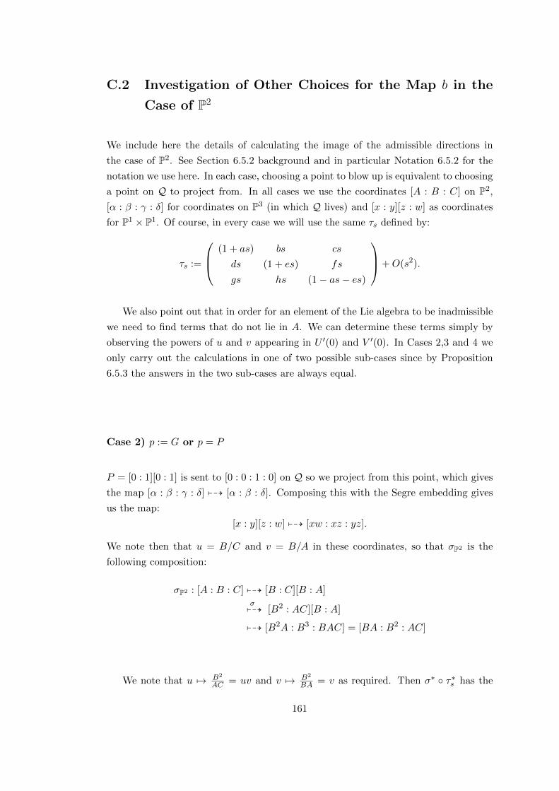
C.2 Investigation of Other Choices for the Map b in the
Case of P2
We include here the details of calculating the image of the admissible directions in
the case of P2. See Section 6.5.2 background and in particular Notation 6.5.2 for the
notation we use here. In each case, choosing a point to blow up is equivalent to choosing
a point on Q to project from. In all cases we use the coordinates [A : B : C] on P2,
[α : β : γ : δ] for coordinates on P3 (in which Q lives) and [x : y][z : w] as coordinates
for P1 × P1. Of course, in every case we will use the same τs defined by:
τs :=
(1 + as) bs cs
ds (1 + es) fs
gs hs (1− as− es)
+O(s2).
We also point out that in order for an element of the Lie algebra to be inadmissible
we need to find terms that do not lie in A. We can determine these terms simply by
observing the powers of u and v appearing in U ′(0) and V ′(0). In Cases 2,3 and 4 we
only carry out the calculations in one of two possible sub-cases since by Proposition
6.5.3 the answers in the two sub-cases are always equal.
Case 2) p := G or p = P
P = [0 : 1][0 : 1] is sent to [0 : 0 : 1 : 0] on Q so we project from this point, which gives
the map [α : β : γ : δ] 799K [α : β : δ]. Composing this with the Segre embedding gives
us the map:
[x : y][z : w] 799K [xw : xz : yz].
We note then that u = B/C and v = B/A in these coordinates, so that σP2 is the
following composition:
σP2 : [A : B : C] 799K [B : C][B : A]
7 σ99K [B2 : AC][B : A]
799K [B2A : B3 : BAC] = [BA : B2 : AC]
We note that u 7→ B2
AC = uv and v 7→ B2
BA = v as required. Then σ∗ ◦ τ∗s has the
161
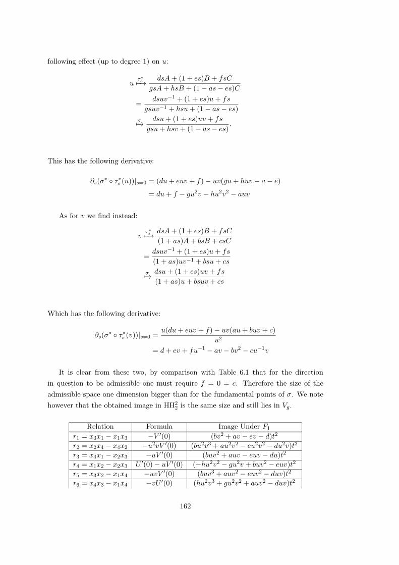
following effect (up to degree 1) on u:
uτ∗s7−→ dsA+ (1 + es)B + fsC
gsA+ hsB + (1− as− es)C
=dsuv−1 + (1 + es)u+ fs
gsuv−1 + hsu+ (1− as− es)σ7−→ dsu+ (1 + es)uv + fs
gsu+ hsv + (1− as− es).
This has the following derivative:
∂s(σ∗ ◦ τ∗s (u))|s=0 = (du+ euv + f)− uv(gu+ huv − a− e)
= du+ f − gu2v − hu2v2 − auv
As for v we find instead:
vτ∗s7−→ dsA+ (1 + es)B + fsC
(1 + as)A+ bsB + csC
=dsuv−1 + (1 + es)u+ fs
(1 + as)uv−1 + bsu+ cs
σ7−→ dsu+ (1 + es)uv + fs
(1 + as)u+ bsuv + cs
Which has the following derivative:
∂s(σ∗ ◦ τ∗s (v))|s=0 =
u(du+ euv + f)− uv(au+ buv + c)
u2
= d+ ev + fu−1 − av − bv2 − cu−1v
It is clear from these two, by comparison with Table 6.1 that for the direction
in question to be admissible one must require f = 0 = c. Therefore the size of the
admissible space one dimension bigger than for the fundamental points of σ. We note
however that the obtained image in HH22 is the same size and still lies in Vg.
Relation Formula Image Under F1
r1 = x3x1 − x1x3 −V ′(0) (bv2 + av − ev − d)t2
r2 = x2x4 − x4x2 −u2vV ′(0) (bu2v3 + au2v2 − eu2v2 − du2v)t2
r3 = x4x1 − x2x3 −uV ′(0) (buv2 + auv − euv − du)t2
r4 = x1x2 − x2x3 U ′(0)− uV ′(0) (−hu2v2 − gu2v + buv2 − euv)t2
r5 = x3x2 − x1x4 −uvV ′(0) (buv3 + auv2 − euv2 − duv)t2
r6 = x4x3 − x1x4 −vU ′(0) (hu2v3 + gu2v2 + auv2 − duv)t2
162

Case 3) p ∈ X \ {P, F} or p ∈ Y \ {G,Q}
Let p = [0 : 1][1 : M ] ∈ X \ {P, F}, where M ∈ K∗. The point [0 : 1][1 : M ]
corresponds to [0 : 0 : M : 1] on Q so we project from this point. This is then the map
[α : β : γ : δ] 799K [α : β : γ −Mδ]. Composing this with the Segre embedding gives us
the map:
[x : y][z : w] 799K [xw : xz : yw −Myz].
Then u = A−MBC and v = B/A in these coordinates, so that σP2 is the following
composition:
σP2 : [A : B;C] 799K [A−MB : C][B : A]
7 σ99K [AB −MB2 : AC][B : A]
799K [A2B −MB2A : AB2 −MB3 : A2C −MBAC]
= [A2B : AB2 : A2C]
We note that
u 7→ A2B −MAB2
A2C= (
A2 −MAB
AC)(B
A) = uv
and
v 7→ AB2
BA2= v
as required. Also, the following formula is very helpful in simplifying the following
expression and is easily derivable from the above:
C
A= (1−Mv)u−1
Then σ∗ ◦ τ∗s has the following effect (up to degree 1) on v:
vτ∗s7−→ dsA+ (1 + es)B + fsC
(1 + as)A+ bsB + csC
=ds+ (1 + es)v + fs(1−Mv)u−1
(1 + as) + bsv + cs(1−Mv)u−1
=dsu+ (1 + es)uv + fs(1−Mv)
(1 + as)u+ bsuv + cs(1−Mv)
σ7−→ dsuv + (1 + es)uv2 + fs(1−Mv)
(1 + as)uv + bsuv2 + cs(1−Mv)
163

Which has the following derivative:
∂s(σ∗ ◦ τ∗s (v))|s=0 =
uv(duv + euv2 + f(1−Mv))− uv2(auv + buv2 + c(1−Mv))
u2v2
= d+ ev + f(1−Mv)u−1v−1 − av + buv2 + c(1−Mv)u−1
From this formula we can deduce immediately that for this to be admissible we require
f, c and b to be 0. As for u,
uτ∗s7−→ (1 + as)A−M(dsA+ (1 + es)B)
gsA+ hsB + (1− as− es)C
=(1 + as)−M(ds+ (1 + es)v)
gs+ hsv + (1− as− es)(1−Mv)u−1
σ7−→ (1 + as)−M(ds+ (1 + es)v)
gs+ hsv + (1− as− es)(1−Mv)u−1v−1
In the following we set:
χ = (a−Md−Mev − (1−Mv)(g + hv + (−a− e)(1−Mv)u−1v−1)).
Then the derivative is as follows:
∂s(σ∗ ◦ τ∗s (u))|s=0 =
(1−Mv)u−1v−1χ
((1−Mv)u−1v−1)2
=a−Md−Mev − guv − huv2 + (−a− e)(1−Mv)
(1−Mv)u−1v−1
Now from this formula we can see that in fact all of the terms must be zero, since
they will be multiplied by the term (1−Mv)−1 and no such term lies in A.
Case 4) p ∈ Z \ {P,Q} or p ∈W \ {F,G}
If p ∈ Z \ {P,Q} then we can write it as p = [1 : M ][0 : 1] for some M ∈ K∗.[1 : M ][0 : 1] is sent to [1 : 0 : M : 0] on Q so we project from this point. This is then
the map [α : β : γ : δ] 799K [β : γ −Mα : δ]. Composing this with the Segre embedding
gives us the map:
[x : y][z : w] 799K [xz : yw −Mxw : yz].
164

Then that u = AC and v = C−MA
B in these coordinates, so that σP2 is the following
composition:
σP2 : [A : B;C] 799K [A : C][C −MA : B]
7 σ99K [A(C −MA) : CB][C −MA : B]
799K [A(C −MA)2 : CB2 −MAB(C −MA) : CB(C −MA)]
We note that
u 7→ A(C −MA)2
CB(C −MA)= (
A
C)(C −MA
B) = uv
and
v 7→ CB(C −MA)−MA(C −MA)2
CB2 −MAB(C −MA)=
(CB −MA(C −MA))(C −MA)
B(CB −MA(C −MA))v
as required. Also, the following formula is very helpful in simplifying the following
expression and is easily derivable from the above:
B
C= (1−Mu)v−1
Then σ∗ ◦ τ∗s has the following effect (up to degree 1) on v:
vτ∗s7−→ gsA+ hsB + (1− as− es)C −M((1 + as)A+ bsB + csC)
dsA+ (1 + es)B + fsC
=gsu+ hs(1−Mu)v−1 + (1− as− es)−M((1 + as)u+ bs(1−Mu)v−1 + cs)
dsu+ (1 + es)(1−Mu)v−1 + fs
=gsuv + hs(1−Mu) + (1− as− es)v −M((1 + as)uv + bs(1−Mu) + csv)
dsuv + (1 + es)(1−Mu) + fsv
σ7−→ gsuv2 + hs(1−Muv) + (1− as− es)v −M((1 + as)uv2 + bs(1−Muv) + csv)
dsuv2 + (1 + es)(1−Muv) + fsv
We let F (s) and G(s) represent the numerator and denominator respectively. Then
the following intermediate values will expedite the calculation of the derivative:
F (0) = v(1−Muv),
F ′(0) = guv2 + h(1−Muv)− av − ev −Mauv2 − bM(Muv) + cvM
G(0) = 1−Muv, G′(0) = duv2 + e(1−Muv) + fv
165

So the derivative is as follows:
∂s(σ∗ ◦ τ∗s (v))|s=0 =
(1−Muv)F ′(0)− v(1−Muv)G′(0)
(1−Muv)2
=1
1−Muv(F ′(0)− vG′(0))
= guv2
1−Muv+ h− ev(−2 +Muv)
1−Muv− av(1 +Muv)
1−Muv
− bM + cvM
1−Muv− d uv3
1−Muv− f v2
1−Muv
From this formula we can deduce immediately that for this to be admissible we require
all of the parameters to be 0 except perhaps b and h.
As for the calculation on u,
uτ∗s7−→ (1 + as)A+ bsB + csC
gsA+ hsB + (1− as− es)C
=A+ bsB
hsB + C
=u+ bs(1−Mu)v−1
hs(1−Mu)v−1 + 1
σ7−→ uv + bs(1−Muv)v−1
hs(1−Muv)v−1 + 1
Which has the following derivative:
∂s(σ∗ ◦ τ∗s (u))|s=0 = b(1−Muv)v−1 − h(1−Muv)u
Since we require that F1(x1x2−x2x3) = (U ′(0)−uV ′(0)t2) ∈ A (see Table 6.1), we
can see that this implies that b = 0 as well. However, h is free to be set as one wishes.
Whatever the value of h however, the infinitesimal deformations obtained lie in Vg.
Case 5)
See Section 6.5.2 for the calculations in this case.
166

Appendix D
Calculations Relevant to
Deformations of Aq Arising from
Quantised Geometric
Automorphisms of Kq(u, v)
D.1 Calculation of F1 applied to the Relations of Aq
We include here the full derivations of F1 applied to the relations of Aq. This supple-
ments the work in Section 7.3.1, and the results are collected in Table 7.1.
1. Recall that r1 = x3x1 − x1x3. Therefore we have the following:
F1(r1) = F1(vt2 − tvt) = vt2 − v(1 + as)t2
=− svat2
2. Recall that r2 = x4x2 − qx2x4 and that σ ◦ τs(u) = uvfs(v). Therefore we have
the following:
F1(r2) = F1(uvtut− qutuvt)
=uvuvfs(v)t2 − qu2vfs(v)(1 + as)vt2
s
∣∣∣∣s=0
=u2q(1 + λs)v2fs(v)t2 − qu2(1 + as)v2fs(v)t2
s
∣∣∣∣s=0
= (qλu2v2 − qau2v2)t2
167
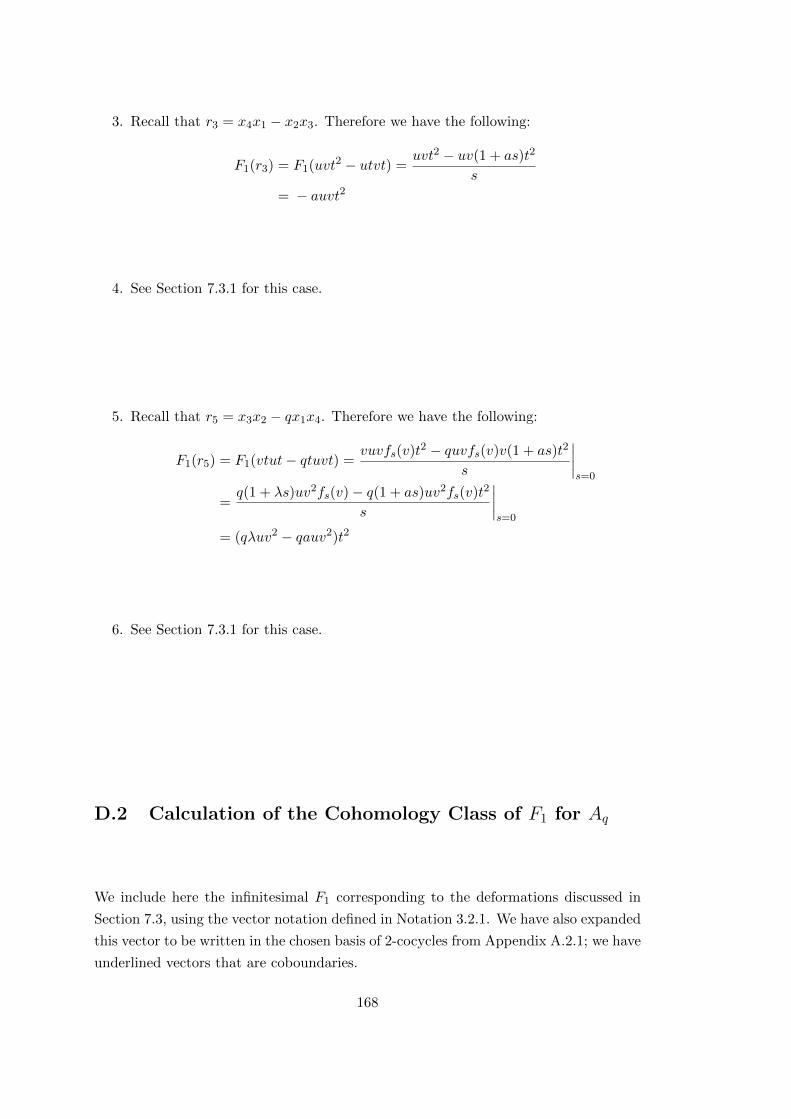
3. Recall that r3 = x4x1 − x2x3. Therefore we have the following:
F1(r3) = F1(uvt2 − utvt) =uvt2 − uv(1 + as)t2
s
= − auvt2
4. See Section 7.3.1 for this case.
5. Recall that r5 = x3x2 − qx1x4. Therefore we have the following:
F1(r5) = F1(vtut− qtuvt) =vuvfs(v)t2 − quvfs(v)v(1 + as)t2
s
∣∣∣∣s=0
=q(1 + λs)uv2fs(v)− q(1 + as)uv2fs(v)t2
s
∣∣∣∣s=0
= (qλuv2 − qauv2)t2
6. See Section 7.3.1 for this case.
D.2 Calculation of the Cohomology Class of F1 for Aq
We include here the infinitesimal F1 corresponding to the deformations discussed in
Section 7.3, using the vector notation defined in Notation 3.2.1. We have also expanded
this vector to be written in the chosen basis of 2-cocycles from Appendix A.2.1; we have
underlined vectors that are coboundaries.
168

a
−x1x3
−qx2x4
−x2x3
−x2x3
−qx1x4
0
+ b
0
0
0
x2x1
0
−x2x3
+ c
0
0
0
x2x3
0
−x1x4
+d
q
0
0
0
qx1x4
0
−x3x4
+ qλ
0
x2x4
0
0
x1x4
0
= a
−
x1x3
0
0
x2x3
qx1x4
0
− q
0
x2x4
0
0
x1x4
0
−
0
0
x2x3
0
−qx1x4
0
+ b
−
0
0
−x2x1
−x2x1
x2x3
x2x3
−
0
(1− q)x22
x2x1
0
−qx2x3
0
+ (1− q)
0
x22
0
0
x2x3
0
+ qλ
0
x2x4
0
0
x1x4
0
+ c
0
0
x2x3
x2x3
−qx1x4
−x1x4
−
0
0
x2x3
0
−qx1x4
0
+d
q
0
0
x1x4
qx1x4
−qx3x4
−x3x4
+
0
(1− q)x24
−x1x4
0
x3x4
0
− (1− q)
0
x24
0
0
x3x4
0
D.3 Calculation of the Cohomology Class of F1 for A
We include here the infinitesimal F1 corresponding to the deformations discussed in
Section 7.3.2, using the vector notation defined in Notation 3.2.1. We have also ex-
panded this vector to be written in the chosen basis of 2-cocycles from Appendix A.1.1;
169
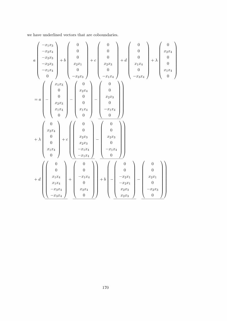
we have underlined vectors that are coboundaries.
a
−x1x3
−x2x4
−x2x3
−x2x3
−x1x4
0
+ b
0
0
0
x2x1
0
−x2x3
+ c
0
0
0
x2x3
0
−x1x4
+ d
0
0
0
x1x4
0
−x3x4
+ λ
0
x2x4
0
0
x1x4
0
= a
−
x1x3
0
0
x2x3
x1x4
0
−
0
x2x4
0
0
x1x4
0
−
0
0
x2x3
0
−x1x4
0
+ λ
0
x2x4
0
0
x1x4
0
+ c
0
0
x2x3
x2x3
−x1x4
−x1x4
−
0
0
x2x3
0
−x1x4
0
+ d
0
0
x1x4
x1x4
−x3x4
−x3x4
+
0
0
−x1x4
0
x3x4
0
+ b
−
0
0
−x2x1
−x2x1
x2x3
x2x3
−
0
0
x2x1
0
−x2x3
0
170
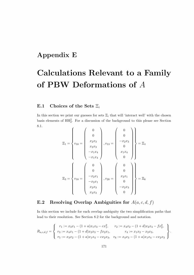
Appendix E
Calculations Relevant to a Family
of PBW Deformations of A
E.1 Choices of the Sets Ξi
In this section we print our guesses for sets Ξi that will ‘interact well’ with the chosen
basis elements of HH22. For a discussion of the background to this please see Section
8.1.
Ξ1 =
v10 =
0
0
x2x3
x2x3
−x1x4
−x1x4
, v13 =
0
0
−x2x3
0
x1x4
0
= Ξ4
Ξ3 =
v18 =
0
0
−x2x1
−x2x1
x2x3
x2x3
, v20 =
0
0
x2x1
0
−x2x3
0
= Ξ6
E.2 Resolving Overlap Ambiguities for A(a, c, d, f)
In this section we include for each overlap ambiguity the two simplification paths that
lead to their resolution. See Section 8.2 for the background and notation.
Ra,c,d,f =
r1 := x3x1 − (1 + a)x1x3 − cx2
1, r2 := x4x2 − (1 + d)x2x4 − fx22,
r3 := x4x1 − (1 + d)x2x3 − fx2x1, r4 := x1x2 − x2x3,
r5 := x3x2 − (1 + a)x1x4 − cx2x3, r6 := x4x3 − (1 + a)x1x4 − cx2x3
.
171
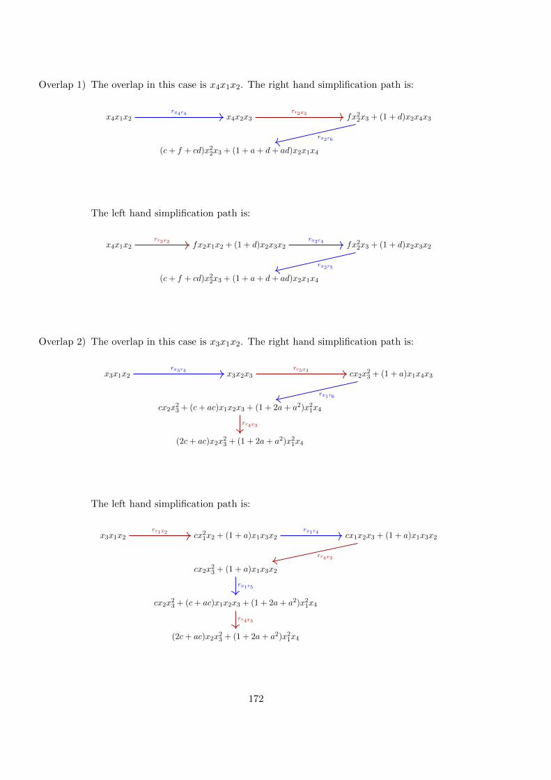
Overlap 1) The overlap in this case is x4x1x2. The right hand simplification path is:
x4x1x2 x4x2x3 fx22x3 + (1 + d)x2x4x3
(c+ f + cd)x22x3 + (1 + a+ d+ ad)x2x1x4
rx4r4 rr2x3
rx2r6
The left hand simplification path is:
x4x1x2 fx2x1x2 + (1 + d)x2x3x2 fx22x3 + (1 + d)x2x3x2
(c+ f + cd)x22x3 + (1 + a+ d+ ad)x2x1x4
rr3x2 rx2r4
rx2r5
Overlap 2) The overlap in this case is x3x1x2. The right hand simplification path is:
x3x1x2 x3x2x3 cx2x23 + (1 + a)x1x4x3
cx2x23 + (c+ ac)x1x2x3 + (1 + 2a+ a2)x2
1x4
(2c+ ac)x2x23 + (1 + 2a+ a2)x2
1x4
rx3r4 rr5x3
rx1r6
rr4x3
The left hand simplification path is:
x3x1x2 cx21x2 + (1 + a)x1x3x2 cx1x2x3 + (1 + a)x1x3x2
cx2x23 + (1 + a)x1x3x2
cx2x23 + (c+ ac)x1x2x3 + (1 + 2a+ a2)x2
1x4
(2c+ ac)x2x23 + (1 + 2a+ a2)x2
1x4
rr1x2 rx1r4
rr4x3
rx1r5
rr4x3
172
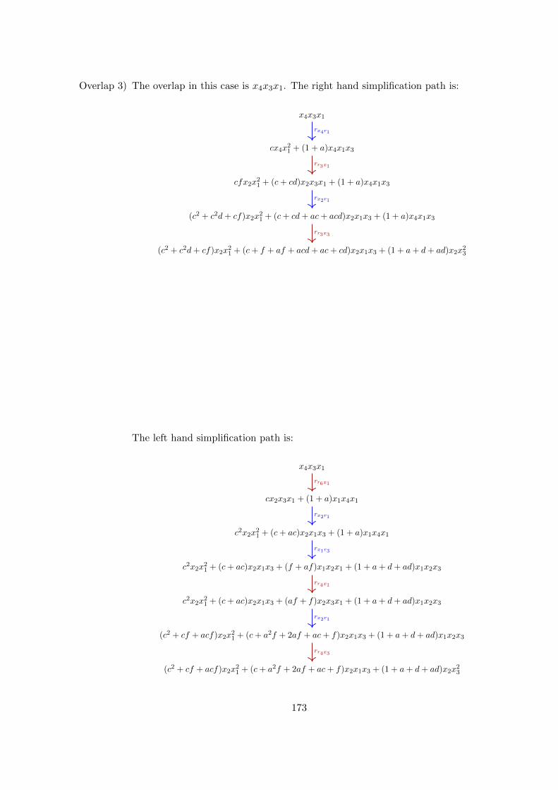
Overlap 3) The overlap in this case is x4x3x1. The right hand simplification path is:
x4x3x1
cx4x21 + (1 + a)x4x1x3
cfx2x21 + (c+ cd)x2x3x1 + (1 + a)x4x1x3
(c2 + c2d+ cf)x2x21 + (c+ cd+ ac+ acd)x2x1x3 + (1 + a)x4x1x3
(c2 + c2d+ cf)x2x21 + (c+ f + af + acd+ ac+ cd)x2x1x3 + (1 + a+ d+ ad)x2x
23
rx4r1
rr3x1
rx2r1
rr3x3
The left hand simplification path is:
x4x3x1
cx2x3x1 + (1 + a)x1x4x1
c2x2x21 + (c+ ac)x2x1x3 + (1 + a)x1x4x1
c2x2x21 + (c+ ac)x2x1x3 + (f + af)x1x2x1 + (1 + a+ d+ ad)x1x2x3
c2x2x21 + (c+ ac)x2x1x3 + (af + f)x2x3x1 + (1 + a+ d+ ad)x1x2x3
(c2 + cf + acf)x2x21 + (c+ a2f + 2af + ac+ f)x2x1x3 + (1 + a+ d+ ad)x1x2x3
(c2 + cf + acf)x2x21 + (c+ a2f + 2af + ac+ f)x2x1x3 + (1 + a+ d+ ad)x2x
23
rr6x1
rx2r1
rx1r3
rr4x1
rx2r1
rr4x3
173

Overlap 4) The overlap in this case is x4x3x2. The right hand simplification path is:
x4x3x2
cx4x2x3 + (1 + a)x4x1x4
cfx22x3 + (c+ cd)x2x4x3 + (1 + a)x4x1x4
(c2 + c2d+ cf)x22x3 + (c+ cd+ ac+ acd)x2x1x4 + (1 + a)x4x1x4
(c2 + c2d+ cf)x22x3 + (c+ f + af + acd+ ac+ cd)x2x1x4 + (1 + a+ d+ ad)x2x3x4
rx4r5
rr2x3
rx2r6
rr3x4
The left hand simplification path is:
x4x3x2
cx2x3x2 + (1 + a)x1x4x2
c2x22x3 + (c+ ac)x2x1x4 + (1 + a)x1x4x2
c2x22x3 + (c+ ac)x2x1x4 + (f + af)x1x
22 + (1 + a+ d+ ad)x1x2x4
c2x22x3 + (c+ ac)x2x1x4 + (af + f)x2x3x2 + (1 + a+ d+ ad)x1x2x4
(c2 + cf + acf)x22x3 + (c+ a2f + 2af + ac+ f)x2x1x4 + (1 + a+ d+ ad)x1x2x4
(c2 + cf + acf)x22x3 + (c+ a2f + 2af + ac+ f)x2x1x4 + (1 + a+ d+ ad)x2x3x4
rr6x2
rx2r5
rx1r2
rr4x2
rx2r5
rr4x4
For an interpretation of these results please see the proof of Theorem 8.2.1.
174
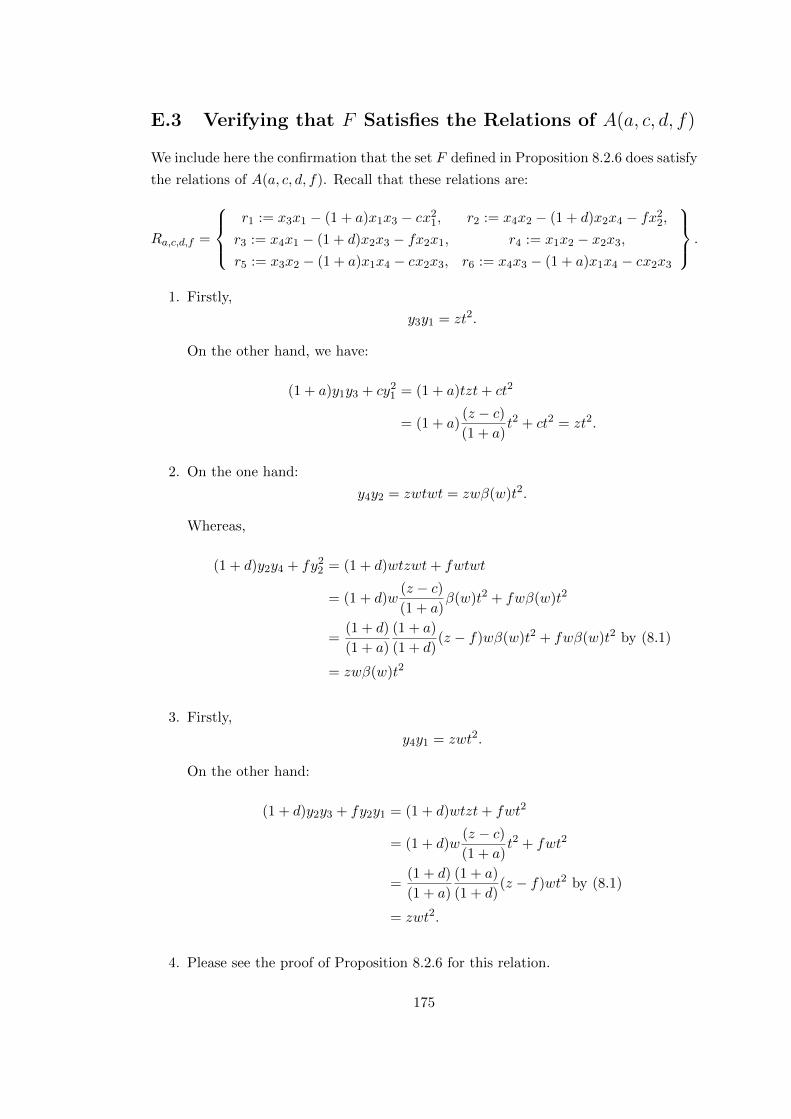
E.3 Verifying that F Satisfies the Relations of A(a, c, d, f)
We include here the confirmation that the set F defined in Proposition 8.2.6 does satisfy
the relations of A(a, c, d, f). Recall that these relations are:
Ra,c,d,f =
r1 := x3x1 − (1 + a)x1x3 − cx2
1, r2 := x4x2 − (1 + d)x2x4 − fx22,
r3 := x4x1 − (1 + d)x2x3 − fx2x1, r4 := x1x2 − x2x3,
r5 := x3x2 − (1 + a)x1x4 − cx2x3, r6 := x4x3 − (1 + a)x1x4 − cx2x3
.
1. Firstly,
y3y1 = zt2.
On the other hand, we have:
(1 + a)y1y3 + cy21 = (1 + a)tzt+ ct2
= (1 + a)(z − c)(1 + a)
t2 + ct2 = zt2.
2. On the one hand:
y4y2 = zwtwt = zwβ(w)t2.
Whereas,
(1 + d)y2y4 + fy22 = (1 + d)wtzwt+ fwtwt
= (1 + d)w(z − c)(1 + a)
β(w)t2 + fwβ(w)t2
=(1 + d)
(1 + a)
(1 + a)
(1 + d)(z − f)wβ(w)t2 + fwβ(w)t2 by (8.1)
= zwβ(w)t2
3. Firstly,
y4y1 = zwt2.
On the other hand:
(1 + d)y2y3 + fy2y1 = (1 + d)wtzt+ fwt2
= (1 + d)w(z − c)(1 + a)
t2 + fwt2
=(1 + d)
(1 + a)
(1 + a)
(1 + d)(z − f)wt2 by (8.1)
= zwt2.
4. Please see the proof of Proposition 8.2.6 for this relation.
175

5. Firstly,
y3y2 = ztwt = zβ(w)t2.
Whereas,
(1 + a)y1y4 + cy2y3 = (1 + a)ztwt+ cwtzt
= (1 + a)(z − c)(1 + a)
β(w)t2 + cw(z − c)(1 + a)
t2
= (z − c)β(w)t2 + cβ(w)t2 by (8.2)
= zβ(w)t2. (E.1)
6.
y4y3 = zwtzt = zwβ(z)t2 = zβ(w)t2 by (8.2).
By (E.1) this equals (1 + a)y1y4 + cy2y3 as required.
Therefore we may conclude that the yi satisfy the defining relations of A(a, c, d, f).
176
References
[AC99] V. A. Artamonov and P. M. Cohn, The skew field of rational functions on
the quantum plane, J. Math. Sci. (New York) 93 (1999), no. 6, 824–829,
Algebra, 11. MR 1698756 (2000f:16052)
[AD95] J. Alev and F. Dumas, Automorphismes de certains completes du corps
de Weyl quantique, Collect. Math. 46 (1995), no. 1-2, 1–9. MR 1366124
(96j:12004)
[AD96] , Rigidite des plongements des quotients primitifs minimaux de
Uq(sl(2)) dans l’algebre quantique de Weyl-Hayashi, Nagoya Math. J. 143
(1996), 119–146. MR 1413010
[Art96] M. Artin, Deformation theory, Unpublished Lecture Notes, 1996.
[Art97] , Some problems on three-dimensional graded domains, Representa-
tion theory and algebraic geometry (Waltham, MA, 1995), London Math.
Soc. Lecture Note Ser., vol. 238, Cambridge Univ. Press, Cambridge, 1997,
pp. 1–19. MR 1477464
[Bea96] Arnaud Beauville, Complex algebraic surfaces, second ed., London Mathe-
matical Society Student Texts, vol. 34, Cambridge University Press, Cam-
bridge, 1996, Translated from the 1978 French original by R. Barlow,
with assistance from N. I. Shepherd-Barron and M. Reid. MR 1406314
(97e:14045)
[Ber78] George M. Bergman, The diamond lemma for ring theory, Adv. in Math.
29 (1978), no. 2, 178–218. MR 506890 (81b:16001)
[BG96] Alexander Braverman and Dennis Gaitsgory, Poincare-Birkhoff-Witt the-
orem for quadratic algebras of Koszul type, J. Algebra 181 (1996), no. 2,
315–328. MR 1383469 (96m:16012)
[BGTV03] Jose Bueso, Jose Gomez-Torrecillas, and Alain Verschoren, Algorithmic
methods in non-commutative algebra, Mathematical Modelling: Theory and
177
Applications, vol. 17, Kluwer Academic Publishers, Dordrecht, 2003, Ap-
plications to quantum groups. MR 2006329 (2005c:16069)
[Cam] Chris Campbell, Polygnome, http://www.github.com/campbellC/polygnome.
[Dev15] The Sage Developers, Sage Mathematics Software (Version 6.5), 2015,
http://www.sagemath.org.
[DI09] Igor V. Dolgachev and Vasily A. Iskovskikh, Finite subgroups of the plane
Cremona group, Algebra, arithmetic, and geometry: in honor of Yu. I.
Manin. Vol. I, Progr. Math., vol. 269, Birkhauser Boston, Inc., Boston,
MA, 2009, pp. 443–548. MR 2641179 (2011c:14032)
[Dol82] Igor Dolgachev, Weighted projective varieties, Group actions and vector
fields (Vancouver, B.C., 1981), Lecture Notes in Math., vol. 956, Springer,
Berlin, 1982, pp. 34–71. MR 704986 (85g:14060)
[EH00] David Eisenbud and Joe Harris, The geometry of schemes, Graduate Texts
in Mathematics, vol. 197, Springer-Verlag, New York, 2000. MR 1730819
(2001d:14002)
[Fox93] Thomas F. Fox, An introduction to algebraic deformation theory, J. Pure
Appl. Algebra 84 (1993), no. 1, 17–41. MR 1195416
[Fry14] Sian Fryer, The q-division ring and its fixed rings, J. Algebra 402 (2014),
358–378. MR 3160427
[Gat14] Andreas Gathmann, Algebraic geometry, http://www.mathematik.
uni-kl.de/~gathmann/class/alggeom-2014/main.pdf, 2014.
[Ger63] Murray Gerstenhaber, The cohomology structure of an associative ring,
Ann. of Math. (2) 78 (1963), 267–288. MR 0161898 (28 #5102)
[Ger64] , On the deformation of rings and algebras, Ann. of Math. (2) 79
(1964), 59–103. MR 0171807 (30 #2034)
[Gia11] Anthony Giaquinto, Topics in algebraic deformation theory, Higher struc-
tures in geometry and physics, Progr. Math., vol. 287, Birkhauser/Springer,
New York, 2011, pp. 1–24. MR 2762537
[GW04] K. R. Goodearl and R. B. Warfield, Jr., An introduction to noncommuta-
tive Noetherian rings, second ed., London Mathematical Society Student
Texts, vol. 61, Cambridge University Press, Cambridge, 2004. MR 2080008
(2005b:16001)
178
[Har77] Robin Hartshorne, Algebraic geometry, Springer-Verlag, New York-
Heidelberg, 1977, Graduate Texts in Mathematics, No. 52. MR 0463157
(57 #3116)
[Hoc45] G. Hochschild, On the cohomology groups of an associative algebra, Ann. of
Math. (2) 46 (1945), 58–67. MR 0011076 (6,114f)
[HSSA14] Estanislao Herscovich, Andrea Solotar, and Mariano Suarez-Alvarez, PBW-
deformations and deformations a la Gerstenhaber of N -Koszul algebras, J.
Noncommut. Geom. 8 (2014), no. 2, 505–539. MR 3275040
[KL00] Gunter R. Krause and Thomas H. Lenagan, Growth of algebras and
Gelfand-Kirillov dimension, revised ed., Graduate Studies in Mathematics,
vol. 22, American Mathematical Society, Providence, RI, 2000. MR 1721834
(2000j:16035)
[KNS58] K. Kodaira, L. Nirenberg, and D. C. Spencer, On the existence of deforma-
tions of complex analytic structures, Ann. of Math. (2) 68 (1958), 450–459.
MR 0112157
[KS58] K. Kodaira and D. C. Spencer, On deformations of complex analytic struc-
tures. I, II, Ann. of Math. (2) 67 (1958), 328–466. MR 0112154
[Moy49] J. E. Moyal, Quantum mechanics as a statistical theory, Proc. Cambridge
Philos. Soc. 45 (1949), 99–124. MR 0029330
[MR01] J. C. McConnell and J. C. Robson, Noncommutative Noetherian rings, re-
vised ed., Graduate Studies in Mathematics, vol. 30, American Mathemat-
ical Society, Providence, RI, 2001, With the cooperation of L. W. Small.
MR 1811901 (2001i:16039)
[New42] M. H. A. Newman, On theories with a combinatorial definition of “equiva-
lence.”, Ann. of Math. (2) 43 (1942), 223–243. MR 0007372
[NvO82] C. Nastasescu and F. van Oystaeyen, Graded ring theory, North Holland,
Amsterdam, 1982.
[NW14] Cris Negron and Sarah Witherspoon, An alternate approach to the Lie
bracket on Hochschild cohomology, arXiv:1406.0036, 2014.
[PP05] Alexander Polishchuk and Leonid Positselski, Quadratic algebras, University
Lecture Series, vol. 37, American Mathematical Society, Providence, RI,
2005. MR 2177131
179

[Pri70] Stewart B. Priddy, Koszul resolutions, Trans. Amer. Math. Soc. 152 (1970),
39–60. MR 0265437 (42 #346)
[Rog] D. Rogalski, Lecture notes for course on noncommutative projective geom-
etry, www.math.ucsd.edu/~drogalsk/msri-notes-lec1-5.pdf.
[Rog09] , GK-dimension of birationally commutative surfaces, Trans. Amer.
Math. Soc. 361 (2009), no. 11, 5921–5945. MR 2529919 (2010j:14008)
[Ros95] Guido Rossum, Python reference manual, Tech. report, Amsterdam, The
Netherlands, The Netherlands, 1995.
[RS09] D. Rogalski and J. T. Stafford, A class of noncommutative projective sur-
faces, Proc. Lond. Math. Soc. (3) 99 (2009), no. 1, 100–144. MR 2520352
(2010j:14007)
[RS12] D. Rogalski and Susan J. Sierra, Some projective surfaces of GK-dimension
4, Compos. Math. 148 (2012), no. 4, 1195–1237. MR 2956041
[Ski08] Steven S. Skiena, The algorithm design manual, 2nd ed., Springer Publish-
ing Company, Incorporated, 2008.
[SVdB01] J. T. Stafford and M. Van den Bergh, Noncommutative curves and noncom-
mutative surfaces, Bull. Amer. Math. Soc. (N.S.) 38 (2001), no. 2, 171–216.
MR 1816070 (2002d:16036)
[Sze99] Balasz Szendroi, The unbearable lightness of deformation theory, http://
people.maths.ox.ac.uk/szendroi/defth.pdf, 1999.
[VdB94] Michel Van den Bergh, Noncommutative homology of some three-
dimensional quantum spaces, Proceedings of Conference on Algebraic Ge-
ometry and Ring Theory in honor of Michael Artin, Part III (Antwerp,
1992), vol. 8, 1994, pp. 213–230. MR 1291019
[Wei94] Charles A. Weibel, An introduction to homological algebra, Cambridge Stud-
ies in Advanced Mathematics, vol. 38, Cambridge University Press, Cam-
bridge, 1994. MR 1269324 (95f:18001)
[YZ06] Amnon Yekutieli and James J. Zhang, Homological transcendence degree,
Proc. London Math. Soc. (3) 93 (2006), no. 1, 105–137. MR 2235944
(2007d:12003)
180
Index
A, 2
A(a, c, d, f), 131
Aq, 36, 120
Vg, 80
Vq, 80, 131
Vu, 80
BG, see Bergman graph
ν, 45
m1, 43
m2, 62, 72
Admissible, see Admissible direction
Admissible direction, 84
Associator, 25
Bar complex, 13, 26, 41
Bar resolution, see Bar complex
Bergman graph, 44, 45, 77
Birationally commutative, 19
Birationally equivalent, 19
Compatible ordering, 42
Cremona group, 84, 118
Diamond, 53
Enveloping algebra, 13
Finitely graded, 19
Flat family, 22, 37, 132
Formal deformation, 21, 23
Function field, see Function skew field
Function skew field, 19, 137
Gelfand-Kirillov dimension, 17, 20, 138
Gerstenhaber bracket, 26, 72
GK-dimension, see Gelfand-Kirillov dimen-
sion
Graded quotient ring, 19, 137
Hilbert series, 18
Hochschild cohomology, 22
Infinitesimal, see Infinitesimal deformation
Infinitesimal deformation, 23, 83, 91, 120
Interfere, 51
Koszul algebra, 13, 20, 85, 91
Koszul complex, 14, 41, 91, 153
Koszul resolution, see Koszul complex
Left Stitch, see Stitch
Noncommutative projective surface, see Non-
commutative surface
Noncommutative surface, 19, 133
Obstruction, 26
Overlap ambiguity, 16, 53, 131
Partial monoid ordering, 42
PBW algebra, 15, 72, 131
PBW order, 41
PBW reduced, see PBW order
Polygnome, 30, 153
Primary obstruction, 26
Quantum Cremona group, 118
181

Reduction sequence, 15
Reduction system, 15
Resolvable, 16
Right stitch, see Stitch
Sage, 29, 30, 33
Simplification path, 45, 131
Stitch, 52
Translation, 51
182
![Commutative Algebra - Cornell Universitypi.math.cornell.edu/.../partiii/files/commalgnotes.pdf · 2018-08-23 · Commutative algebra is about commutative rings: Z, k[x1,...,xn], etc](https://img.pdfslide.net/doc/110x75/5f157dcc3ba58c0b6a7eac81/commutative-algebra-cornell-2018-08-23-commutative-algebra-is-about-commutative.jpg)


![Gröbner Bases in Commutative bner Bases in Commutative Algebra Viviana Ene Jürgen Herzog American Mathematical Society ... [M86] H.Matsumura,Commutative ringtheory,CambridgeUniversityPress,1986.Authors:](https://img.pdfslide.net/doc/110x75/5aa0fbd37f8b9a0d158ef3cd/grbner-bases-in-commutative-bases-in-commutative-algebra-viviana-ene-jrgen-herzog.jpg)


![Commutative Algebra - GitHub Pages · 2021. 4. 8. · Matsumura’s Commutative Ring Theory [Mat89], or his other less known book Eisenbud’s Commutative Algebra with a view towards](https://img.pdfslide.net/doc/110x75/612a0ee35d7cd36a002d5c1c/commutative-algebra-github-pages-2021-4-8-matsumuraas-commutative-ring.jpg)


![arXiv:0704.2503v4 [math.QA] 2 Jul 2015 · in [H1, H2, H3] the deformation functors assign to an artinian commutative ring an ∞-groupoid. Kan simplicial sets and fibrant groupoids](https://img.pdfslide.net/doc/110x75/5e9a6f22cf9782594a446f35/arxiv07042503v4-mathqa-2-jul-2015-in-h1-h2-h3-the-deformation-functors.jpg)